USING COAMPS NWP MODEL IN GNSS TOMOGRAPHY

JUNIORSTAV 2009 6.2 Practical Aspects of Geodesy and Cartography

1

USING COAMPS NWP MODEL IN GNSS TOMOGRAPHY

Witold Rohm1

Abstract The numerical weather prediction (NWP) models are widely used for forecasting the weather on daily basis. One of

the most popular and reliable amongst them is COAMPS (Coupled Ocean Atmospheric Mesoscale Prediction System), model calculates weather parameters as an solution of the partial differential set of equations. The GNSS tomography is a method to obtain the distribution of sensed quantity from integrated measure. In this case the sensed quantity is a refractivity in a voxel while the integrated measure is SWD (Slant Wet Delay). There are four potential use of NWP model in the tomography first is to validate the obtained wet refractivity second is to convert from wet refractivity to humidity with the help of pressure and temperature, third is to derive vertical gradient of the meteorological parameters for the use with local data, and fourth is to use NWP obtained refractivities as an initial guess .This paper gives short insight into these four research area, together with short description of both COAMPS and GNSS tomography model.

Keywords GNSS meteorology, tomography, NWP models

1 INTRODUCTION The GNSS meteorology is rapidly developing branch of geoscience. The possible of usage GPS as an additional

data source for meteorological applications is a consequence of signal delay when traveling through the troposphere. The varying part of Zenith Tropospheric Delay (ZTD) is linked with water vapour [9]. Thus knowing the part linked with water vapour might be some measure of the water vapour itself. The technique to obtain the 3D distribution of water vapour from GNSS observations is tomography. This technique suffers from lack of additional reference data. here the potential usage of NWP data as an additional data source has been shown.

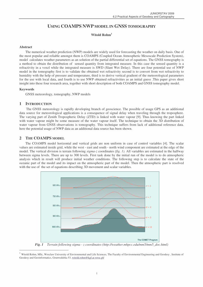
2 THE COAMPS MODEL The COAMPS model horizontal and vertical grids are non uniform in case of control variables [4]. The scalar

values are estimated inside grid, while the west - east and south - north wind component are estimated at the edge of the model. The vertical division is terrain following sigma-z coordinates (fig. 1). All variables are estimated in the halfway between sigma levels. There are up to 300 levels. First task done by the initial run of the model is to do atmospheric analysis which in result will produce initial weather conditions. The following step is to calculate the state of the oceanic part of the model and its impact on the atmospheric part of the model. Then the atmospheric part is resolved with the use of the set of equations describing 3D movement and scalar variables.

Fig. 1 Terrain following sigma - z coordinates (http://weather.mhpcc.edu/mm5/mm5_doc.html)

1 Witold Rohm, MSc, Wroclaw University of Environmental and Life Sciences, The Faculty of Environmental Engineering and Geodesy , Institute of Geodesy and Geoinformatics, Grunwaldzka 53, [email protected]/


2

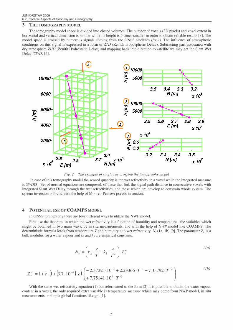
3 THE TOMOGRAPHY MODEL The tomography model space is divided into closed volumes. The number of voxels (3D pixels) and voxel extent in

horizontal and vertical dimension is similar while its height is 5 times smaller in order to obtain reliable results [8]. The model space is crossed by numerous signals coming from the GNSS satellites (fig.2). The influence of atmospheric conditions on this signal is expressed in a form of ZTD (Zenith Tropospheric Delay). Subtracting part associated with dry atmosphere ZHD (Zenith Hydrostatic Delay) and mapping back into direction to satellite we may get the Slant Wet Delay (SWD) [5].

Fig. 2 The example of single ray crossing the tomography model

In case of this tomography model the sensed quantity is the wet refractivity in a voxel while the integrated measure is SWD[3]. Set of normal equations are composed, of these that link the signal path distance in consecutive voxels with integrated Slant Wet Delay through the wet refractivities, and these which are develop to constrain whole system. The system inversion is found with the help of Moore - Penrose pseudo inversion.

4 POTENTIAL USE OF COAMPS MODEL In GNSS tomography there are four different ways to utilize the NWP model. First use the theorem, in which the wet refractivity is a function of humidity and temperature - the variables which

might be obtained in two main ways, by in situ measurements, and with the help of NWP model like COAMPS. The deterministic formula leads from temperature T and humidity e to wet refractivity Nv (1a, 1b) [9]. The parameter Zv is a bulk modulus for a water vapour and k2 and k3 are empirical constants.

(1a)

( )( ) ��

�

�

��

�

�

⋅⋅⋅−⋅⋅−

⋅⋅⋅⋅−

−−−−−

34

21341

107.75141

710.7922.23366102.37321103.711

T+

TT+e+e+=Z v

(1b)

With the same wet refractivity equation (1) but reformatted to the form (2) it is possible to obtain the water vapour content in a voxel, the only required extra variable is temperature measure which may come from NWP model, in situ measurements or simple global functions like gpt [1].

1232

−⋅��

��

� ⋅+⋅= vv ZTe

kTe

kN


3

1

232

−

��

��

�⋅⋅Tk

+Tk

ZN=e vv (2)

Although the annual variations in these models are well preserved (fig. 3), the diurnal and semi diurnal changeability is not resolved at all [7]

Fig. 3 The comparison between meteorological model gpt (yellow) and observations (red and blue) for

temperature(left panel) and pressure(right panel) .Station MATE (Matera) Please note in pressure not modeled spring drop.

The third possibility is to obtain the variability (3) of the parameters from the NWP model. Which are three spatio - temporal gradients (temperature, pressure, humidity) and with the help of locally measured parameters populate the tomography model space with meteorological quantities.

��

��

�

∂∂

∂∂∇

nxf

,,xf

=f �

1

(3)

For each parameter the equation (3) might be rewritten to form (4) where f is a either temperature or pressure or humidity and x, y, z are Cartesian coordinates.

( ) ��

��

�

∂∂

∂∂

∂∂∇

zf

,yf

,xf

=zy,x,f (4)

The vertical gradients from COAMPS model hour 3 PM of pressure temperature and humidity has been shown at the figure 4.

Fig. 3 Picture presents gradients estimated by COAMPS model. The left panel shows pressure gradient in vertical coordinates, middle panel is temperature gradient while right panel shows water vapour gradient. Please note that

these gradients are far from standard gradient profiles.


4

Fourth way to use data from NWP model is to obtain initial guess for the inversion module Nva (5). Then in the estimation process determine only corrections to the initial values of wet refractivity Nv after [2] with minor modifications. The matrices Cy Ca are measurements error covariance and apriori error covariance respectively.

( ) ( )vayT

ayT

vav NASWDCAC+ACA+N=N ⋅−⋅⋅⋅⋅⋅ −−−− 1111 (5)

5 ERROR DISCUSSION To asses the required precision the random error propagation has been performed based on the equation (2). The

term Zv has been dropped in order to simplify the calculations. Priori to these operations the impact of neglecting or not the term has been performed. The Zv obtain value one, when the water vapour is assumed the perfect gas, or greater than one in all other cases. As seen from the figure 4 the impact is on the order of 1% of relative error, regardless NWP data (close to real) or UNB3 data (rather mean profile) [6] has been used as an input for equation 1.

Fig. 4 The comparison between different sources of wet refractivity with and without Zv component. The red dots presents data from UNB3 while green stars COAMPS NWP data.

The error budged calculation was based on several assumptions the best possible temperature measurement is of the

order of 1K and decreasing pattern has been applied with increasing height fig.5 top left panel. Similar effect might be observed for wet refractivity the best possible precision is 1 mm/km weakening with elevation, fig.5 top right panel. The resulting errors for wet refractivity is pictured at the middle panel of fig 5. Bottom panel shows error histogram, the maximal and most frequent error is on the order of 5 hPa which is almost 50% of relative error.


5

Fig. 5 The error budget. Top panels shows input errors of temperature and wet refractivity, middle panel presents the resulting water vapour and water vapour error bars while bottom panel shows error histogram.

6 OUTLINE The wet refractivity obtained in bottom section of the model with precision around 1mm/km gives small errors, but the amount of water vapour with height is decreasing so model sensitivity with height has to increase. The minimum temperature precision is around 2K which is possible to achieve. General model of weather phenomena distribution are to weak in local scale in short time periods, the changeability of the system is much more complicated than might be foreseen with the simple model. The accurate in situ measurements has a very good agreement with COAMPS model what might be the point not to define the gradient from the model but take the model variables as they are. In this case in situ measurements will be used as a monitoring values to prevent from discrepancies. Another comment is that in situ measurements has to be carefully investigated priori to usage - there might be a large error budget due to insolation, or sensor decalibration. Only professional measurements inside meteorological cages guarantee high data accuracy and therefore usage in further analysis.

7 ACKNOWLEDGMENT This work has been financed as a research project N520 014 31/2095 from the Polish science funds for the period 2006-2008 and the Wroclaw Centre of Networking and Supercomputing (http://www.wcss.wroc.pl/) computational grant using Matlab Software License No: 101979

Literature [1] BOEHM, J., HEINKELMANN, R., SCHUH, H., Short Note: A global model of pressure and temperature for

geodetic applications. Journal of Geodesy: Springer, 2007, 679–683.

[2] CHAMPOLLIONA, C. *,MASSONA F., BOUINB M.-N, WALPELSDORF A., DOERDLINGERA E., BOCKD O., VAN BAELEN, J., GPS Water Vapour Tomography: Preliminary results from the ESCOMPTE Field Experiment, Atmospheric Research: Springer, 2005, 253--274

[3] FLORES A., RUFFINI G., RIUS A., 4D tropospheric tomography using GPS slant wet delays, Ann. Geophysicae: EGU, 2000, 223-234.

[4] HODUR, Richard M., The Coupled Ocean/Atmosphere Mesoscale Prediction System (COAMPS), Oceanography : The Oceanography Society, 2002, 88-98,

[5] KLEIJER F. Troposphere Modeling and Filtering for Precise GPS Leveling. PhD thesis. Delft University, The Netherlands, 2004.

[6] LEANDRO, R., SANTOS, M. LANGLEY, R.B., UNB Neutral Atmosphere Models: Development and Performance, Technical Report, http://gauss.gge.unb.ca/UNB3/frame4.html, 2006

[7] ROHM, W., BOSY, J., The quality of meteorological observations and tropospheric delay from EPN/IGS permanent stations located in the Sudety mountains and in the adjacent areas. Acta Geodynamica et Geomaterialia: Institute of the Rock Structure and Mechanics, 2007. 145–152.

[8] ROHM, Witold, BOSY, Jaroslaw, Local tomography troposphere model over mountains area, submitted to Atmospheric Research: Elsevier, 2008

[9] THAYER G. D., An Improved Equation for the Radio Refractive Index of Air, Radio Science: AGU, 1974, 803-807.

[10] http://weather.mhpcc.edu/mm5/mm5_doc.html

Reviewer/Rezensent

Jaroslaw Bosy, Wroclaw University of Environmental and Life Sciences, The Faculty of Environmental Engineering and Geodesy , Institute of Geodesy and Geoinformatics, prof., Grunwaldzka 53, +48 71 3205688, [email protected]

Documents

USING COAMPS NWP MODEL IN GNSS TOMOGRAPHY