Embed Size (px)
Citation preview

Using Parallel Mesh Partitioning Strategies to Improve the Performance
of Tau3P, an Electromagnetic Field Solver
Michael M. Wolf, University of Illinois, Urbana-Champaign; Ali Pinar, Lawrence Berkeley National
Laboratory; Karen D. Devine, Sandia National Laboratories; Adam Guetz, Nate Folwell and Kwok
Ko, Stanford Linear Accelerator Center
SIAM PP04 – February 25, 2004San Francisco, CA

2
Outline
• Motivation• Brief Description of Tau3P• Tau3P Performance• Partitioning Results• Port Grouping• Future Work

3
Challenges in E&M Modeling of Accelerators
• Accurate modeling essential for modern accelerator design
• Reduces Design Cost• Reduces Design Cycle
• Conformal meshes (Unstructured grid)• Large, complex electromagnetic structures
• 100’s of millions of DOFs• Small beam size
• Large number of mesh points• Long run time
• Parallel Computing needed (time and storage)

4
Next Linear Collider (NLC)
Cell to cell variation of order microns to suppress short range wakes by detuning

5
• NLC X-band structure showing damage in the structure cells after high power test
• Theoretical understanding of underlying processes lacking so realistic simulation is needed
End-to-end NLC Structure Simulation

6
Parallel Time-Domain Field Solver – Tau3P
Coupler Matching
R TReflectedIncident
Transmitted
Coupler Matching
Wakefield Calculations Rise Time Effects

7
Parallel Time-Domain Field Solver – Tau3P
The DSI formulation yields:
∫∫∫∫∫
∫∫∫
•+•∂∂=•
•∂∂−=•
*** dAjdA
tDdsH
dAtBdsE
eAhhAe
E
Hvv
vv
⋅⋅=+
⋅⋅=+
β
α • α, β are constants proportional to dt• AH,AE are matrices• Electric fields on primary grid• Magnetic fields on embedded dual grid• Leapfrog time advancement• (FDTD) for orthogonal grids
• Follows evolution of E and H fields inside accelerator cavity• DSI method on non-orthogonal meshes

8
Tau3P Implementation
Example of Distributed Mesh
Typical Distributed Matrix
• Very Sparse Matrices– 4-20 nonzeros per row
• 2 Coupled Matrices (AH,AE)• Nonsymmetric (Rectangular)

9
Parallel Performance of Tau3P (ParMETIS)
2.02.8
3.9 4.45.7
6.8
9.2
Parallel Speedup
• 257K hexahedrons• 11.4 million non-zeroes

10
Communication in Tau3P (ParMETIS Partitioning)
Communication vs. Computation Process Boundaries

11
Flexibility in Tau3P Mesh Partitioning
• Long simulation times– Tens of thousands of CPU hours
• Problem initialization short• Most time spent in time advancement
– Millions of time steps• Static mesh partitioning• Willing to pay HIGH price upfront for
increased performance of solver

12
Partitioning Methods
• Using Zoltan (Sandia National Laboratory) • Tried Several Mesh Partitioning Methods:
– Graph Partitioning Algorithms• ParMETIS
– Geometric Partitioning Algorithms (1D/2D/3D)• Recursive Coordinate Bisection (RCB)• Recursive Inertial Bisection (RIB)• Hilbert Space-Filling Curve (HSFC)

13
Several Partitioning Methods

14
1D (RCB-1D(z)) Partitioning

15
5 Cell RDDS (8 processors) Partitioning
9038 2030 32 5387.3 sHSFC-3D
7927 1570 18 3282.4 sRIB-3D
11961 1965 26 5343.0 sRCB-3D
14363 3128 14 2218.5 sRCB-1D (z)
2909 585 14 3288.5 sParMETIS
Sum Bound. Objs
Max Bound. Objs
Sum Adj. Procs
Max Adj. Procs
Tau3P Runtime
2.0 ns runtimeIBM SP3 (NERSC)

16
5 Cell RDDS (32 processors) Partitioning
26684 1279 202 10 272.2 sHSFC-3D
20156 808 162 8 266.8 sRIB-3D
24321 1404 208 10 373.2 sRCB-3D
63510 2683 66 3 67.7 sRCB-1D (z)
16405 731 134 8 165.5 sParMETIS
Sum Bound. Objs
Max Bound. Objs
Sum Adj. Procs
Max Adj. Procs
Tau3P Runtime
2.0 ns runtimeIBM SP3 (NERSC)
17
H60VG3 (“real” structure)
55 cells (w/ coupler)1,122,445 elements

18
H60VG3 RDDS Partitioning (w/o port grouping)
1.0 ns runtimeIBM SP3 (NERSC)
Processors
Max. A
dj. Procs
Parallel E
fficiency
-- ParMETIS Adj. Procs
-- RCB-1D Adj. Procs
ParMETIS Efficiency
RCB-1D Efficiency

19
RCB-1D Scalability Leveling Off

20
Coupler Port Grouping Complication

21
Coupler Port Grouping Complication

22
H60VG3 RDDS Partitioning (w/ coupler port grouping)
1.0 ns runtimeIBM SP3 (NERSC)
Processors
Max. A
dj. Procs
Parallel E
fficiency
-- RCB-1D Adj. Procs
ParMETIS Efficiency
RCB-1D Efficiency
-- ParMETIS Adj. Procs

23
Constrained Mesh Partitioning

24
RDDS Coupler Cell Constrained Partition (16 procs)
7 RIB-3D 5 RIB-2D-yz
14 RIB-2D-xz 6 RIB-2D-xy 8 RCB-3D 6 RCB-2D-yz 14 RCB-2D-xz 5 RCB-2D-xy
14 RCB-1D-z 8 ParMETIS
14 HSFC-3D Max Adj. ProcsMethod
25
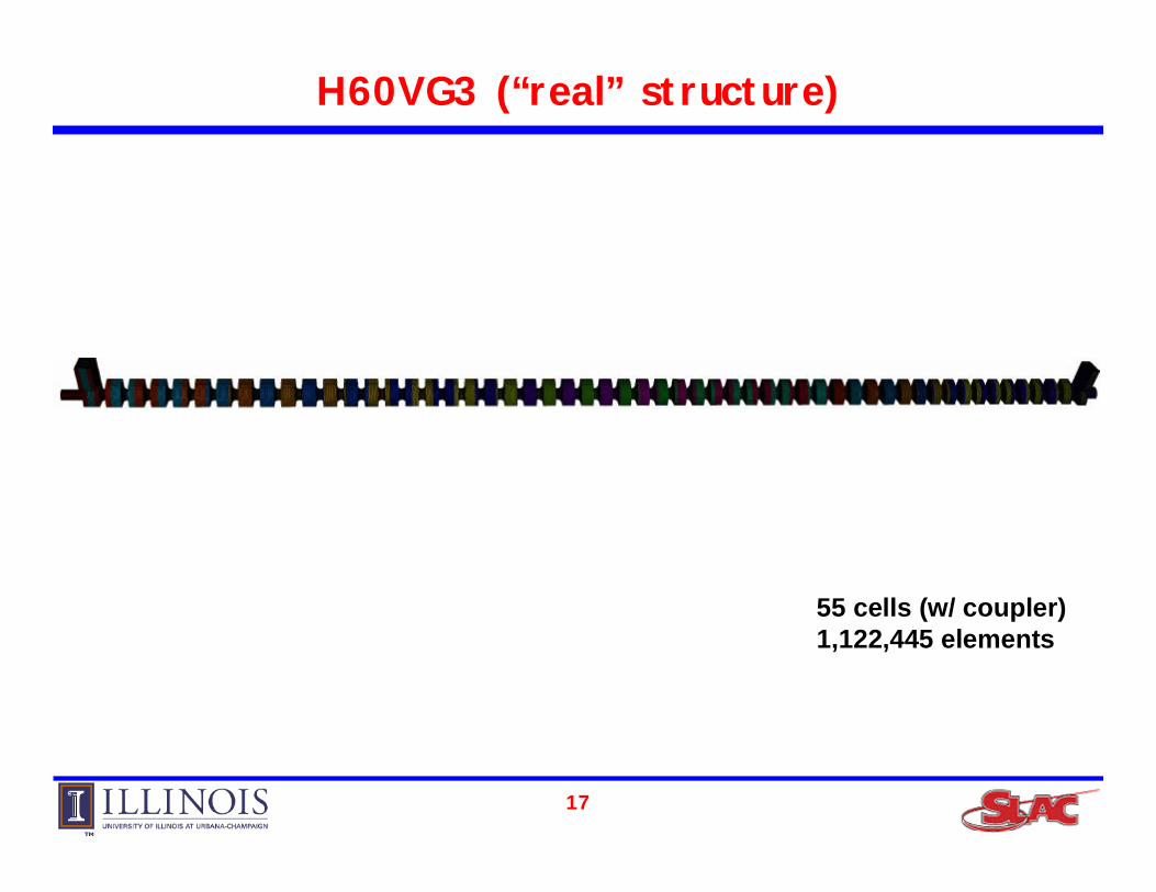
RDDS Coupler Cell Constrained Partition (32 procs)
12 RIB-3D 6 RIB-2D-yz
29 RIB-2D-xz 7 RIB-2D-xy 11 RCB-3D 7 RCB-2D-yz
29 RCB-2D-xz 7 RCB-2D-xy
29 RCB-1D-z 14 ParMETIS 17 HSFC-3D
Max Adj. ProcsMethod

26
“U” Partitioning (Ongoing Work)
• RCB 1D Partitioning• Remap coordinates • Partition based on distance from curve.

27
“U” Partitioning of 5 cell (32 processors)

28
“U” Partitioning vs. “Z” Partitioning
-- RCB-1D-Z Adj. Procs Run Tim
e (s)
Max. A
dj. Procs
Processors
RCB-1D-Z Run Time
-- RCB-1D-U Adj. Procs
RCB-1D-U Run Time

29
Future Work
• “U” or “Fork” Partitioning• Stitching Multiple Partitions Together• Method Competition• Connectivity into geometric methods• Local partitioning• Other methods

30
Acknowledgements
• SNL– Karen Devine, et al.
• LBNL– Ali Pinar
• SLAC (ACD)– Adam Guetz, Cho Ng, Nate Folwell, Lixin
Ge, Greg Schussman, Kwok Ko
• Work supported by U.S. DOE ASCR & HENP Divisions under contract DE-AC0376SF00515


![Centrifuge: Integrated Lease Management and Partitioning ... · system. Relying on client republishing is the approach taken by the Live Mesh services [22], and we describe this in](https://img.pdfslide.net/doc/110x75/5f426c58eed2fd1b192ea5b1/centrifuge-integrated-lease-management-and-partitioning-system-relying-on.jpg)


![Object Partitioning for Point Clouds - cv-foundation.org€¦ · [3]Evangelos Kalogerakis, Aaron Hertzmann, and Karan Singh. Learning 3d mesh segmentation and labeling. ACM Transactions](https://img.pdfslide.net/doc/110x75/5f3b2cb5f33d536aae787741/object-partitioning-for-point-clouds-cv-3evangelos-kalogerakis-aaron-hertzmann.jpg)