Embed Size (px)
Citation preview
AUTONOMOUS CONTROL OF AN UNSTABLE MODEL
HELICOPTER USING CARRIER PHASE GPS ONLY
a dissertation
submitted to the department of electrical engineering
and the committee on graduate studies
of stanford university
in partial fulfillment of the requirements
for the degree of
doctor of philosophy
By
Andrew Richard Conway
March 1995

c Copyright 1995 by Andrew Richard Conway
All Rights Reserved
ii
I certify that I have read this dissertation and that in my
opinion it is fully adequate, in scope and in quality, as a
dissertation for the degree of Doctor of Philosophy.
Robert H. Cannon, Jr.Department of Aeronautics and Astronautics
(Principal Adviser)
I certify that I have read this dissertation and that in my
opinion it is fully adequate, in scope and in quality, as a
dissertation for the degree of Doctor of Philosophy.
Gene F. FranklinDepartment of Electrical Engineering
I certify that I have read this dissertation and that in my
opinion it is fully adequate, in scope and in quality, as a
dissertation for the degree of Doctor of Philosophy.
Ronald N. BracewellDepartment of Electrical Engineering
Approved for the University Committee
on Graduate Studies:
iii

iv

Abstract
This thesis contains the results of my experiments in using carrier phase Global
Positioning System (GPS) techniques to totally control an inherently unstable model
helicopter for the �rst time. In the process a new algorithm for determining the unknown
integer wavelength o�sets for attitude calculation was devised.
The helicopter is capable of hovering autonomously. It uses four GPS antennas on
the helicopter and a ground reference station to determine position and attitude to
precisions of roughly a centimetre and a degree, both at a ten Hertz update rate.
The new algorithm for integer resolution allows integers to be resolved in a computa-
tionally e�cient manner with fewer satellites in view than previous algorithms, allowing
use in a greater number of applications.
This thesis describes the overall problems, approaches, and philosophy of design,
then contains detailed descriptions of the various logical parts of the project. A descrip-
tion is given of GPS, carrier phase approaches, and how position, velocity, attitude and
attitude rate can be calculated, and a description of the new algorithms that make this
possible. The hardware used in this project is then described, followed by the software
for ight and analysis. The results of ight tests are given, and then some conclusions
and suggestions for further work in this valuable arena are presented. The appendices
contain comprehensive technical details of the hardware and software.
v

vi
Acknowledgements
I would like to thank Professors Robert Cannon and Stephen Rock for their vital
advice, as well as e�orts in �nding funding and experts in a variety of �elds. I would
like to thank Professor Gene Franklin for his help in the EE department.
This was quite a large project, and many people contributed directly to it. Above
all, I would like to thank Robert Cannon for showing me how to manage such a project,
which was something I had no real ability in. Immense thanks go to Steve Morris, heli-
copter virtuoso, who built, maintained and ew the helicopters under trying conditions
and often with little notice, as well as having a large impact upon the control design
and for teaching me about helicopters. Steve's innate conservatism counterbalanced my
overactive optimism well, and let us y a dangerous, fragile object safely and without
major crash. Thanks also to Ben Tigner and Bruce Woodley who saved me a large
quantity of time and frustration by helping with many of the immense number of tasks
that had to be done perfectly to give the helicopter any chance at reliability. Thank
you also for putting up with my poor abilities as a delegator. Similar thanks to Gad
Shelef and Godwin Zhang for their help and skills in mechanical and electronic con-
struction. Thanks also to Gerardo Pardo-Castellote, Eric Olsen, Gordon Hunt, Kortney
Leabourne, HD Stevens, Jay Little�eld and Je� Russakow for helping in the �eld or
other signi�cant actions. Many thanks also to everyone else in the Aerospace Robotics
Laboratory for constant helpful suggestions, especially Larry Pfe�er who seems to know
a little bit about everything.
On the GPS side, I was fortunate to have the GP-B laboratory's GPS experimenters
around. Thanks to Professor Bradford Parkinson, Clark Cohen and Trimble Navigation
for their support of this project. Many thanks to Stu Cobb, Hiro Uematsu and Kurt
Zimmerman for explaining what the black boxes from Trimble were supposed to do.
Especial thanks to Paul Montgomery who worked very closely with me on several parts
of the GPS software, making suggestions, �nding bugs, explaining the contents of the
black boxes, and being almost entirely responsible for the velocity measurements.
This work was funded (and therefore made possible) by the Boeing Company and
vii

NASA Ames Research center. Thanks to Shoreline Amphitheatre for letting RC en-
thusiasts y in in their parking lot, and to NASA Ames for letting us y on an Ames
runway.
Many thanks to the readers, especially R Cannon, who worked so quickly and dili-
gently.
Lastly and perhaps most importantly, thank you to my friends in the Bay Area for
making life here much more pleasant.
viii
Contents
Abstract v
Acknowledgements viii
1 Introduction 1
1.1 What is a robot? : : : : : : : : : : : : : : : : : : : : : : : : : : : : : : : 1
1.2 Why a helicopter? : : : : : : : : : : : : : : : : : : : : : : : : : : : : : : 3
1.3 Why GPS? : : : : : : : : : : : : : : : : : : : : : : : : : : : : : : : : : : 4
1.4 Contributions : : : : : : : : : : : : : : : : : : : : : : : : : : : : : : : : : 5
1.5 Contest : : : : : : : : : : : : : : : : : : : : : : : : : : : : : : : : : : : : 7
1.6 People working on this project : : : : : : : : : : : : : : : : : : : : : : : 10
1.7 Outline of thesis : : : : : : : : : : : : : : : : : : : : : : : : : : : : : : : 13
2 Global Positioning System (GPS) 14
2.1 Terminology : : : : : : : : : : : : : : : : : : : : : : : : : : : : : : : : : : 18
2.2 GPS Receiver data : : : : : : : : : : : : : : : : : : : : : : : : : : : : : : 19
2.3 Assume the integers are known : : : : : : : : : : : : : : : : : : : : : : : 20
2.3.1 On the Size of quantities : : : : : : : : : : : : : : : : : : : : : : : 20
2.3.2 Position : : : : : : : : : : : : : : : : : : : : : : : : : : : : : : : : 22
2.3.3 Velocity : : : : : : : : : : : : : : : : : : : : : : : : : : : : : : : : 24
2.3.4 Attitude : : : : : : : : : : : : : : : : : : : : : : : : : : : : : : : : 27
2.3.5 Pseudo-global attitude solution : : : : : : : : : : : : : : : : : : : 31
2.3.6 Finding the minimum of equation 2.23 : : : : : : : : : : : : : : 32
ix

2.3.7 Attitude Rate : : : : : : : : : : : : : : : : : : : : : : : : : : : : : 38
2.4 Obtaining Integers : : : : : : : : : : : : : : : : : : : : : : : : : : : : : : 38
2.4.1 Position : : : : : : : : : : : : : : : : : : : : : : : : : : : : : : : : 40
2.4.2 Attitude : : : : : : : : : : : : : : : : : : : : : : : : : : : : : : : : 49
3 Hardware 57
3.1 Helicopter : : : : : : : : : : : : : : : : : : : : : : : : : : : : : : : : : : : 57
3.1.1 Actuators : : : : : : : : : : : : : : : : : : : : : : : : : : : : : : : 59
3.2 Helicopter Electronics : : : : : : : : : : : : : : : : : : : : : : : : : : : : 62
3.3 Ground Station Electronics : : : : : : : : : : : : : : : : : : : : : : : : : 66
3.4 Operations : : : : : : : : : : : : : : : : : : : : : : : : : : : : : : : : : : 69
4 Software 73
4.1 Data Flow : : : : : : : : : : : : : : : : : : : : : : : : : : : : : : : : : : : 73
4.1.1 Operational : : : : : : : : : : : : : : : : : : : : : : : : : : : : : : 74
4.1.2 Initialisation : : : : : : : : : : : : : : : : : : : : : : : : : : : : : 78
4.1.3 Data Retrieval : : : : : : : : : : : : : : : : : : : : : : : : : : : : 81
4.1.4 Post-processing : : : : : : : : : : : : : : : : : : : : : : : : : : : : 85
4.2 68HC11 programs : : : : : : : : : : : : : : : : : : : : : : : : : : : : : : 85
4.3 486 software : : : : : : : : : : : : : : : : : : : : : : : : : : : : : : : : : : 87
4.4 Control : : : : : : : : : : : : : : : : : : : : : : : : : : : : : : : : : : : : 89
5 Flight-Test Results 95
5.1 Flight Pro�le : : : : : : : : : : : : : : : : : : : : : : : : : : : : : : : : : 95
5.2 Computer Controlled Portion of Flight : : : : : : : : : : : : : : : : : : : 100
6 Conclusions and Future Work 114
6.1 An aside on Languages : : : : : : : : : : : : : : : : : : : : : : : : : : : : 116
A Helicopter manual 121
A.1 Suppliers : : : : : : : : : : : : : : : : : : : : : : : : : : : : : : : : : : : 121
A.2 Electronic connection : : : : : : : : : : : : : : : : : : : : : : : : : : : : : 121
x
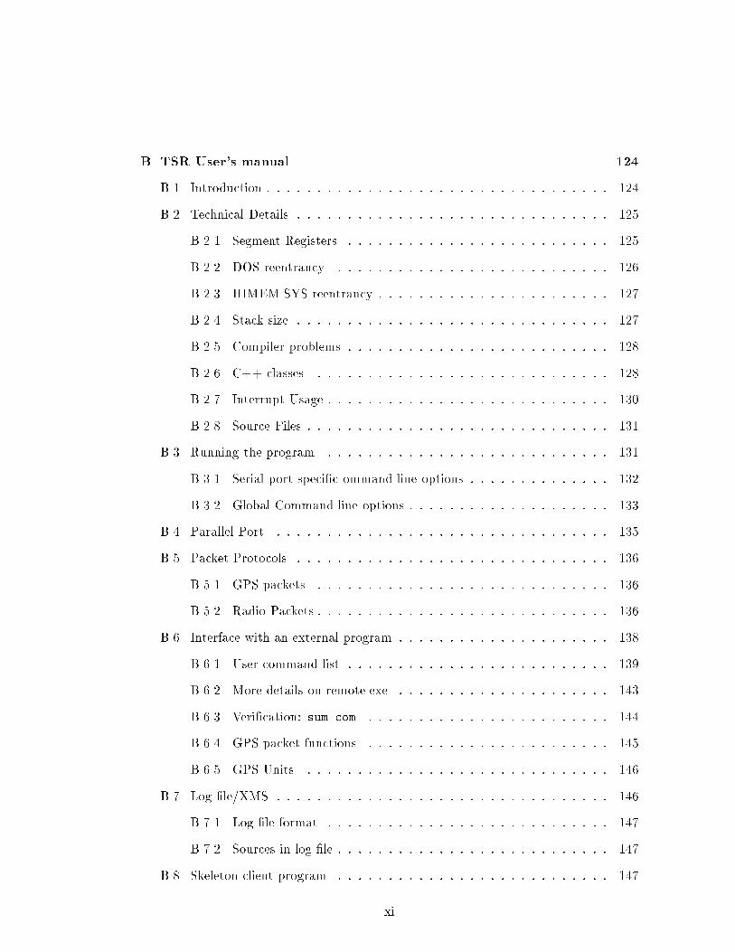
B TSR User's manual 124
B.1 Introduction : : : : : : : : : : : : : : : : : : : : : : : : : : : : : : : : : : 124
B.2 Technical Details : : : : : : : : : : : : : : : : : : : : : : : : : : : : : : : 125
B.2.1 Segment Registers : : : : : : : : : : : : : : : : : : : : : : : : : : 125
B.2.2 DOS reentrancy : : : : : : : : : : : : : : : : : : : : : : : : : : : 126
B.2.3 HIMEM.SYS reentrancy : : : : : : : : : : : : : : : : : : : : : : : 127
B.2.4 Stack size : : : : : : : : : : : : : : : : : : : : : : : : : : : : : : : 127
B.2.5 Compiler problems : : : : : : : : : : : : : : : : : : : : : : : : : : 128
B.2.6 C++ classes : : : : : : : : : : : : : : : : : : : : : : : : : : : : : 128
B.2.7 Interrupt Usage : : : : : : : : : : : : : : : : : : : : : : : : : : : : 130
B.2.8 Source Files : : : : : : : : : : : : : : : : : : : : : : : : : : : : : : 131
B.3 Running the program : : : : : : : : : : : : : : : : : : : : : : : : : : : : 131
B.3.1 Serial port speci�c ommand line options : : : : : : : : : : : : : : 132
B.3.2 Global Command line options : : : : : : : : : : : : : : : : : : : : 133
B.4 Parallel Port : : : : : : : : : : : : : : : : : : : : : : : : : : : : : : : : : 135
B.5 Packet Protocols : : : : : : : : : : : : : : : : : : : : : : : : : : : : : : : 136
B.5.1 GPS packets : : : : : : : : : : : : : : : : : : : : : : : : : : : : : 136
B.5.2 Radio Packets : : : : : : : : : : : : : : : : : : : : : : : : : : : : : 136
B.6 Interface with an external program : : : : : : : : : : : : : : : : : : : : : 138
B.6.1 User command list : : : : : : : : : : : : : : : : : : : : : : : : : : 139
B.6.2 More details on remote.exe : : : : : : : : : : : : : : : : : : : : : 143
B.6.3 Veri�cation: sum.com : : : : : : : : : : : : : : : : : : : : : : : : 144
B.6.4 GPS packet functions : : : : : : : : : : : : : : : : : : : : : : : : 145
B.6.5 GPS Units : : : : : : : : : : : : : : : : : : : : : : : : : : : : : : 146
B.7 Log �le/XMS : : : : : : : : : : : : : : : : : : : : : : : : : : : : : : : : : 146
B.7.1 Log �le format : : : : : : : : : : : : : : : : : : : : : : : : : : : : 147
B.7.2 Sources in log �le : : : : : : : : : : : : : : : : : : : : : : : : : : : 147
B.8 Skeleton client program : : : : : : : : : : : : : : : : : : : : : : : : : : : 147
xi
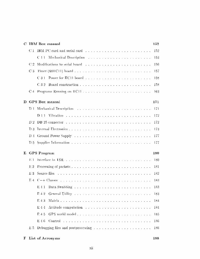
C IBM Box manual 152
C.1 IBM PC card and serial card : : : : : : : : : : : : : : : : : : : : : : : : 152
C.1.1 Mechanical Description : : : : : : : : : : : : : : : : : : : : : : : 153
C.2 Modi�cations to serial board : : : : : : : : : : : : : : : : : : : : : : : : 156
C.3 Timer (68HC11) board : : : : : : : : : : : : : : : : : : : : : : : : : : : : 157
C.3.1 Power for HC11 board : : : : : : : : : : : : : : : : : : : : : : : : 158
C.3.2 Board construction : : : : : : : : : : : : : : : : : : : : : : : : : : 158
C.4 Programs Running on HC11 : : : : : : : : : : : : : : : : : : : : : : : : : 163
D GPS Box manual 171
D.1 Mechanical Description : : : : : : : : : : : : : : : : : : : : : : : : : : : 171
D.1.1 Vibration : : : : : : : : : : : : : : : : : : : : : : : : : : : : : : : 172
D.2 DB 25 connector : : : : : : : : : : : : : : : : : : : : : : : : : : : : : : : 172
D.3 Internal Electronics : : : : : : : : : : : : : : : : : : : : : : : : : : : : : : 173
D.4 Ground Power Supply : : : : : : : : : : : : : : : : : : : : : : : : : : : : 177
D.5 Supplier Information : : : : : : : : : : : : : : : : : : : : : : : : : : : : : 177
E GPS Program 180
E.1 Interface to TSR : : : : : : : : : : : : : : : : : : : : : : : : : : : : : : : 180
E.2 Processing of packets : : : : : : : : : : : : : : : : : : : : : : : : : : : : : 181
E.3 Source �les : : : : : : : : : : : : : : : : : : : : : : : : : : : : : : : : : : 182
E.4 C++ Classes : : : : : : : : : : : : : : : : : : : : : : : : : : : : : : : : : 183
E.4.1 Data Swabbing : : : : : : : : : : : : : : : : : : : : : : : : : : : : 183
E.4.2 General Utility : : : : : : : : : : : : : : : : : : : : : : : : : : : : 183
E.4.3 Matrix : : : : : : : : : : : : : : : : : : : : : : : : : : : : : : : : : 184
E.4.4 Attitude computation : : : : : : : : : : : : : : : : : : : : : : : : 184
E.4.5 GPS world model : : : : : : : : : : : : : : : : : : : : : : : : : : : 185
E.4.6 Control : : : : : : : : : : : : : : : : : : : : : : : : : : : : : : : : 186
E.5 Debugging �les and postprocessing : : : : : : : : : : : : : : : : : : : : : 186
F List of Acronyms 188
xii

Bibliography 191
xiii
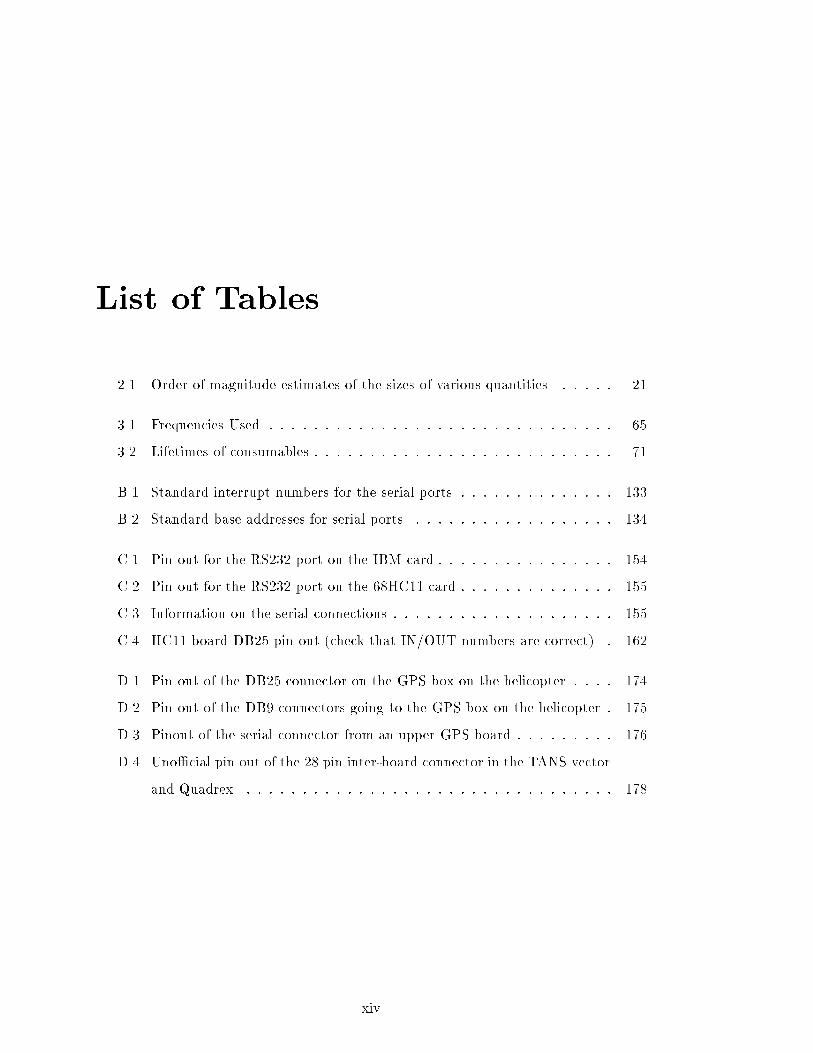
List of Tables
2.1 Order of magnitude estimates of the sizes of various quantities : : : : : 21
3.1 Frequencies Used : : : : : : : : : : : : : : : : : : : : : : : : : : : : : : : 65
3.2 Lifetimes of consumables : : : : : : : : : : : : : : : : : : : : : : : : : : : 71
B.1 Standard interrupt numbers for the serial ports. : : : : : : : : : : : : : : 133
B.2 Standard base addresses for serial ports. : : : : : : : : : : : : : : : : : : 134
C.1 Pin out for the RS232 port on the IBM card : : : : : : : : : : : : : : : : 154
C.2 Pin out for the RS232 port on the 68HC11 card : : : : : : : : : : : : : : 155
C.3 Information on the serial connections : : : : : : : : : : : : : : : : : : : : 155
C.4 HC11 board DB25 pin out (check that IN/OUT numbers are correct) : 162
D.1 Pin out of the DB25 connector on the GPS box on the helicopter : : : : 174
D.2 Pin out of the DB9 connectors going to the GPS box on the helicopter : 175
D.3 Pinout of the serial connector from an upper GPS board : : : : : : : : : 176
D.4 Uno�cial pin out of the 28 pin inter-board connector in the TANS vector
and Quadrex : : : : : : : : : : : : : : : : : : : : : : : : : : : : : : : : : 178
xiv
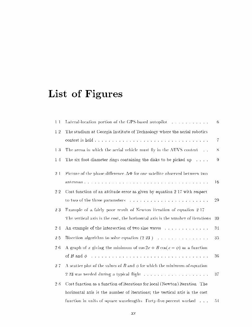
List of Figures
1.1 Lateral-location portion of the GPS-based autopilot. : : : : : : : : : : : 6
1.2 The stadium at Georgia Institute of Technology where the aerial robotics
contest is held : : : : : : : : : : : : : : : : : : : : : : : : : : : : : : : : : 7
1.3 The arena in which the aerial vehicle must y in the AUVS contest. : : 8
1.4 The six foot diameter rings containing the disks to be picked up : : : : 9
2.1 Picture of the phase di�erence �� for one satellite observed between two
antennas : : : : : : : : : : : : : : : : : : : : : : : : : : : : : : : : : : : : 16
2.2 Cost function of an attitude error as given by equation 2.17 with respect
to two of the three parameters. : : : : : : : : : : : : : : : : : : : : : : : 29
2.3 Example of a fairly poor result of Newton iteration of equation 2.17 .
The vertical axis is the cost, the horizontal axis is the number of iterations. 30
2.4 An example of the intersection of two sine waves : : : : : : : : : : : : : 34
2.5 Bisection algorithm to solve equation (2.23 ). : : : : : : : : : : : : : : : 35
2.6 A graph of x giving the minimum of cos 2x +B cos(x+ �) as a function
of B and �. : : : : : : : : : : : : : : : : : : : : : : : : : : : : : : : : : : 36
2.7 A scatter plot of the values of B and � for which the minimum of equation
2.23 was needed during a typical ight. : : : : : : : : : : : : : : : : : : : 37
2.8 Cost function as a function of iterations for local (Newton) iteration. The
horizontal axis is the number of iterations; the vertical axis is the cost
function in units of square wavelengths. Forty-�ve percent worked. : : : 54
xv
2.9 Cost function as a function of iterations for 20 global then local iterations.
The horizontal axis is the number of iterations; the vertical axis is the
cost function in units of square wavelengths. Seventy-three percent worked. 55
2.10 Cost function as a function of iterations for alternating 2 global / 2 local
iterations. The horizontal axis is the number of iterations; the vertical
axis is the cost function in units of square wavelengths. Eighty-six percent
worked. : : : : : : : : : : : : : : : : : : : : : : : : : : : : : : : : : : : : 56
3.1 The helicopter loaded with electronics. : : : : : : : : : : : : : : : : : : : 58
3.2 Hardware needed to start the engine and perform �eld maintenance and
adjustments : : : : : : : : : : : : : : : : : : : : : : : : : : : : : : : : : : 59
3.3 The radio console (with antenna retracted) for controlling an RC helicopter 60
3.4 RC Transmitter mapping from throttle to blade pitch. Units are propor-
tional to servo actuation : : : : : : : : : : : : : : : : : : : : : : : : : : : 61
3.5 The master antenna on the tail of the helicopter. : : : : : : : : : : : : : 63
3.6 The positions of the four GPS antennas on the helicopter and their rela-
tive distances. : : : : : : : : : : : : : : : : : : : : : : : : : : : : : : : : : 64
3.7 The electronic signal connections on board the helicopter : : : : : : : : 67
3.8 The power connections on board the helicopter : : : : : : : : : : : : : : 68
3.9 Ground Equipment : : : : : : : : : : : : : : : : : : : : : : : : : : : : : : 69
3.10 Electronics in the ground station : : : : : : : : : : : : : : : : : : : : : : 70
3.11 The safety shield : : : : : : : : : : : : : : : : : : : : : : : : : : : : : : : 71
3.12 The helicopter taking o�, as seen through the shield. : : : : : : : : : : : 72
4.1 Breakdown into conceptual units of the software running on the 486 on
the helicopter during normal operations. Undashed lines indicate data
movement; Dashed lines indicate computation. This performs the com-
puter control sections in �gure 1.1 . : : : : : : : : : : : : : : : : : : : : : 75
4.2 Breakdown into conceptual units of the software running on the ground
station 486 during normal operations. Lines indicate data movement : : 79
xvi
4.3 Data Flow in the 68HC11 servo control processors. An undashed line
indicates unconditional data ow; a dashed line indicates possible data
ow. : : : : : : : : : : : : : : : : : : : : : : : : : : : : : : : : : : : : : : 80
4.4 Data movement during initialisation for the 486 on the helicopter : : : : 82
4.5 Data movement during initialisation for the ground-station : : : : : : : 83
4.6 Data transfer involved in down-loading ight data from the helicopter 486. 84
4.7 Data movement for the postprocessing software. Undashed lines indicate
data movement; Dashed lines indicate computation. : : : : : : : : : : : 86
4.8 Altitude control loop, with GPS feedback on position and velocity. Gains
are given in terms of percentage of the normal full control actuation.
Based on �gure 1.1 . : : : : : : : : : : : : : : : : : : : : : : : : : : : : : 91
4.9 Heading control loop, with GPS feedback on attitude (yaw). The gain is
given in terms of tail rotor pitch (degrees) per degree of yaw error. Based
upon �gure 1.1 . : : : : : : : : : : : : : : : : : : : : : : : : : : : : : : : 92
4.10 Longitudinal-position / pitch control loop, with GPS feedback on posi-
tion, velocity and attitude (pitch). Speci�c longitudinal version of �gure
1.1 . : : : : : : : : : : : : : : : : : : : : : : : : : : : : : : : : : : : : : : 93
4.11 Lateral position / bank angle control loop, with GPS feedback on posi-
tion, velocity and bank angle. Speci�c form of �gure 1.1 . : : : : : : : : 94
5.1 A test ight performed on 31 Dec 1994. : : : : : : : : : : : : : : : : : : 96
5.2 East component of displacement in ight performed on 31 Dec 1994 : : 97
5.3 East component of velocity in ight performed on 31 Dec 1994 : : : : : 98
5.4 Theta (angle tilted forwards, pitch) in ight performed on 31 Dec 1994 : 98
5.5 Pilot command directly a�ecting pitch in ight performed on 31 Dec 1994 100
5.6 Altitude under computer control in ight performed on 31 Dec 1994 : : 101
5.7 Heading under computer control in ight performed on 31 Dec 1994 : : 101
5.8 Displacement north under computer control in ight performed on 31 Dec
19 94 : : : : : : : : : : : : : : : : : : : : : : : : : : : : : : : : : : : : : : 102
xvii
5.9 Displacement east under computer control in ight performed on 31 Dec
19 94 : : : : : : : : : : : : : : : : : : : : : : : : : : : : : : : : : : : : : : 102
5.10 Autocorrelation of � (roll) signal whilst under computer control and sta-
ble, showing the 11 second period limit cycle. : : : : : : : : : : : : : : : 104
5.11 Pilot throttle commands whilst under computer control : : : : : : : : : 104
5.12 Pilot heading commands whilst under computer control : : : : : : : : : 105
5.13 Pilot pitch commands whilst under computer control : : : : : : : : : : : 105
5.14 Pilot roll commands whilst under computer control : : : : : : : : : : : : 106
5.15 Slew in heading under computer control. : : : : : : : : : : : : : : : : : : 107
5.16 Bank angle � commanded by the computer (with an o�set) from position
feedback versus actual � measurements. Refer to �gures 1.1 and 4.11 . : 109
5.17 A correlation between the time delayed angle command and the observed
� during computer control. : : : : : : : : : : : : : : : : : : : : : : : : : 109
5.18 Altitude under computer control for ight of 31 Jan 1995 : : : : : : : : 110
5.19 Heading under computer control for ight of 31 Jan 1995 : : : : : : : : 111
5.20 North displacement under computer control for ight of 31 Jan 1995 : : 111
5.21 East displacement under computer control for ight of 31 Jan 1995 : : : 112
5.22 Pilot commanded y translation whilst under computer control for ight
of 31 Jan 1995. Each unit of command represents a 31.5 cm change in
the set point. : : : : : : : : : : : : : : : : : : : : : : : : : : : : : : : : : 112
A.1 Location of parts on board the helicopter. : : : : : : : : : : : : : : : : : 122
A.2 LED driver : : : : : : : : : : : : : : : : : : : : : : : : : : : : : : : : : : 123
C.1 Contents of autoexec.bat on the embedded PC : : : : : : : : : : : : : : 153
C.2 Contents of con�g.sys on the embedded PC : : : : : : : : : : : : : : : : 153
C.3 Layout of serial ports on the IBM box. : : : : : : : : : : : : : : : : : : : 154
C.4 Circuit diagram for the HC11 board : : : : : : : : : : : : : : : : : : : : 159
C.5 Circuit diagram for the connector to the HC11 board, radios, Servos and
486. : : : : : : : : : : : : : : : : : : : : : : : : : : : : : : : : : : : : : : 160
C.6 Servo pin out for male connector : : : : : : : : : : : : : : : : : : : : : : 161
xviii

D.1 Power Supply for the GPS box circuit diagram : : : : : : : : : : : : : : 173
D.2 Orientation of the 28 pin connector on the GPS board for table D.4 : : 173
D.3 Orientation of the 34 pin IDC connector on the GPS board 28 pin connector175
D.4 Circuit Diagram for the power supply for the ground based electronics : 179
xix
Chapter 1
Introduction
Much of the history of engineering technology can be viewed as an increase in the abilities
of humans. Mechanical devices can increase a human's precision, speed, leverage, shape,
strength or appendage arrangement. Engines increased humans' total power supply.
Large structures allow humans to bend the world into shapes more useful for humans.
More recently, humans have had access to vast quantities of power: the need for sheer
physical strength in humans is now rare. Much of engineering technology has turned
towards information. Computers and communications allow a human's mind to be more
productive than previously, and there is now little need for humans to perform tedious
calculations. Robots allow humans to get away from having to direct the operations of
machinery themselves.
1.1 What is a robot?
The science of robotics is still very young. In particular, most robots are relatively
simple and non-ambulatory. The exceptions to this rule tend to be teleoperated robots;
that is, robots that are controlled, usually in real time, by a human. Teleoperated robots
allow a human to interact with environments with which a human could not directly
interact and thus serve a vital role; but they are not as potentially powerful as fully
or even partially autonomous robots that can perform a task without full time human
supervision and control.
1
2 CHAPTER 1. INTRODUCTION
It is a little surprising that robots have not had as large an impact upon the world
as many futurists have predicted, given the rapid exponential growth possible with
complete automation, and therefore the enormous economic incentives to build such
devices. There are several reasons for such lack of impact.
Perhaps the most important stumbling block has been the lack of arti�cial intelli-
gence. The muscles and joints of a human body are easily within today's technology to
reproduce | and improve upon | but the ability to do something intelligent then is
rather di�cult.
One step down from full intelligence, and much more feasible today is to enable
robots to perform a small number of short tasks. This has ended up being fairly suc-
cessful, and many tedious tasks have been automated. However, there are still immense
problems with the overwhelming complexity of describing in computer code tasks that
seem quite simple to a human. Complexity also comes into the ability to control systems
that are not very simple. Control theory is quite good for simple perfectly rigid linear
systems, but is still being developed for more complex systems.
One further step down, a robot must be aware of its current state, and the state of
its environment in order to make reasonable future movements, and this turns out to
also be surprisingly di�cult. One of the hardest state variables to measure is position
of the robot in the environment, as there are few physical properties that are intrinsic
to position in an easily computable manner in an arbitrary environment. This lack of
position information makes mobile robots particularly di�cult.
Most animals seem to be able to cope in a world without a direct position sensor
through a variety of sensors such as vision, hearing (including sonar) and smell, and with
an incredibly complex and poorly understood processing stage inside the brain that can
collate enormous quantities of information, cross reference with a complex world view,
and produce a result suitable for tasks such as eating grass, remembering how to get
to the water hole, and killing other animals. This system, while having the undeniable
advantage of working well, is not used directly in robots for several reasons. Firstly,
we do not know how to do it. Secondly, even if we did, modern computers and storage
capabilities may not be up to the task. Thirdly, there are some tasks we may wish done
1.2. WHY A HELICOPTER? 3
by robots that require signi�cantly more accurate measurements. Most importantly,
there are alternatives.
While the typical science �ction characterisation of a robot is a humanoid object1,
there is no more requirement for a robot to have legs rather than wheels, or wings rather
than turboprops, than there is for it to metabolise carbohydrates or proteins rather than
burn high grade hydrocarbons or use electricity stored in myriad ways. Similarly, there
is no reason why robots have to use the same senses as animals when there are other
viable alternatives, such as radio based systems. There are advantages to the animal
approaches: legs can go over rocks, wings are exceedingly e�cient and can be turned on
and o� easily, carbohydrates are readily available and vision accomplishes many other
useful things; but they do not preclude useful robots being built using other technologies.
1.2 Why a helicopter?
This thesis contains the results so far of Stanford's experiments in building an au-
tonomous helicopter as a robot | a long way from C3PO in \Star Wars", but useful
none the less.
The immediate question is \Don't remote control (RC) airplanes and helicopters
already exist", and the answer is of course \Yes." One can buy excellent RC models from
a hobby shop for a reasonable amount of money. However, they are just teleoperated
devices; they could potentially be made signi�cantly easier to use. In particular, RC
helicopters { being inherently unstable { are particularly di�cult to control, and need
a very skilled pilot concentrating full time on ying.
Aerial robots are unlikely to be particularly useful in manufacturing, but they are
useful in transportation, observation, and working in impassable terrain for ground-
based vehicles or hazardous environments like a volcano. Perhaps the most immediate
application to the commercial world is the investigation of power lines for electricity
suppliers | it is di�cult to observe from the ground, and radio controlled helicopters
are very di�cult to y as mentioned previously.
1The word `robot' itself came from a Czechoslovakian play meaning `working man' with overtones ofslavery and monotony, and was popularised by science �ction authors then became commonplace.
4 CHAPTER 1. INTRODUCTION
Helicopters have the signi�cant advantage over winged aircraft in that they can
hover, which is of vital importance for observation-based tasks. Model helicopters do
however come with some severe disadvantages:
� They tend to be unstable with fairly rapid dynamics.
� They are less e�cient than winged aircraft, and thus cannot carry as much payload,
which restricts the amount of electronics and other hardware that can be added.
� Hobby helicopters are limited in size, restricting the payload size to several kilo-
grams.
� They have severe vibration problems, so the control electronics must be very
rugged.
� They do not have much spare volume available for bulky objects.
� They crash easily, spectacularly, and thoroughly.
In this project we used as a basis the largest available hobby store type RC helicopter
as the starting point. It is described in section 3.1.
1.3 Why GPS?
As mentioned previously, position is a physical quantity that is particularly hard to
sense. This is especially true on board an aerial vehicle, as one needs to sense in three
dimensions, and many of the solutions that can be done indoors (such as overhead vision
of the robot, or special markings on the oor or walls) do not work.
Classical solutions involve star tracking (a di�cult method, especially during the
day), dead reckoning using sophisticated inertial measurement devices (expensive, quite
heavy, and prone to drift), and extraordinarily sophisticated (and complex, heavy and
expensive) vision systems.
One source of position information that is starting to become very popular is the
Global Positioning System (GPS), which can be used to measure absolute position
anywhere on the world using microwave radio transmissions from satellites.
1.4. CONTRIBUTIONS 5
Recent developments have made it possible to determine local position with an
accuracy of to centimetres, using GPS carrier phase measurements. (e.g. [8]) This then
has all of the requirements we were looking for in a sensor: light, cheap, fast, drift-free,
accurate and precise.
Using similar methods it is possible to use GPS to measure attitude in real time (e.g.
[12, 11, 9, 17]) by the use of several antennas. While roll and pitch can be measured with
gyroscopes and pendula in a drift-free manner with respect to the direction of gravity in
the helicopter reference system, azimuth is di�cult to measure well (compasses are the
classic instrument, but have problems with local anomalies and magnetic equipment).
Also, using just one sensor (with no moving parts) for all tasks has advantages in terms
of overall system cost and reliability. Thus it was decided to use GPS for computing
attitude as well.
Due to the di�culty of obtaining a drift-free sensor, just using normal, several-metre-
accuracy di�erential GPS has been studied for normal helicopters (e.g. [10]) and is being
used in the emerging �eld of unmanned aerial vehicles in conjunction with other faster,
more-accurate local inertial devices.
GPS is discussed in detail in chapter 2
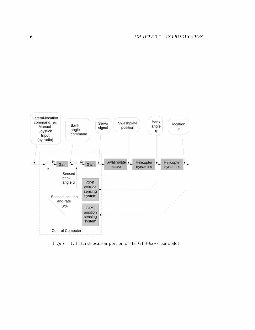
The control system used in the present research is shown (for one degree of freedom)
in schematic form in �gure 1.1. This �gure shows an innermost attitude control loop,
surrounded by a position control loop, with position commanded by the radio console.
1.4 Contributions
The research described in this dissertation has resulted in fundamental experimental
and algorithmic contributions to automatic control that have been demonstrated in
new successful experiments.
� New e�cient algorithms and approaches to use real-time data from GPS sensors
for control of an unstable plant have been developed.
� These new algorithms allowed for the �rst time the full, autonomous control of an
intrinsically unstable model helicopter in hover using only GPS signals to sense
6 CHAPTER 1. INTRODUCTION
+ + Swashplateservo
Helicopterdynamics
Helicopterdynamics
GPSattitudesensingsystem
GPSpositionsensingsystem
Control Computer
Lateral-locationcommand, yc:
Manual Joystick
Input(by radio)
Gain Gain
Sensed location and rate y,y.
.
Sensedbankangle φ
ye
Bankanglecommand
Servosignal
Swashplateposition
Bankangle
φ
locationy
φe
Figure 1.1: Lateral-location portion of the GPS-based autopilot.
1.5. CONTEST 7
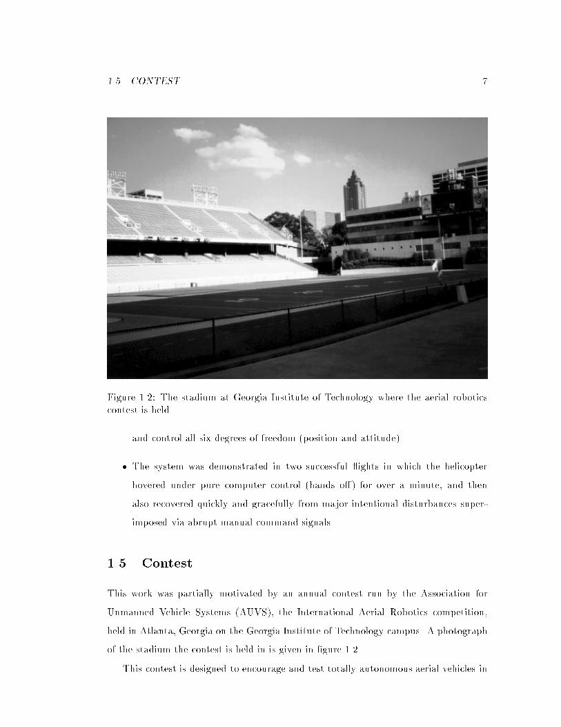
Figure 1.2: The stadium at Georgia Institute of Technology where the aerial roboticscontest is held
and control all six degrees of freedom (position and attitude).
� The system was demonstrated in two successful ights in which the helicopter
hovered under pure computer control (hands o�) for over a minute, and then
also recovered quickly and gracefully from major intentional disturbances super-
imposed via abrupt manual command signals.
1.5 Contest
This work was partially motivated by an annual contest run by the Association for
Unmanned Vehicle Systems (AUVS), the International Aerial Robotics competition,
held in Atlanta, Georgia on the Georgia Institute of Technology campus. A photograph
of the stadium the contest is held in is given in �gure 1.2.
This contest is designed to encourage and test totally autonomous aerial vehicles in
8 CHAPTER 1. INTRODUCTION
Start
Pick up disksDrop off disks
3’ high barrier
15’
15’
60’
120’
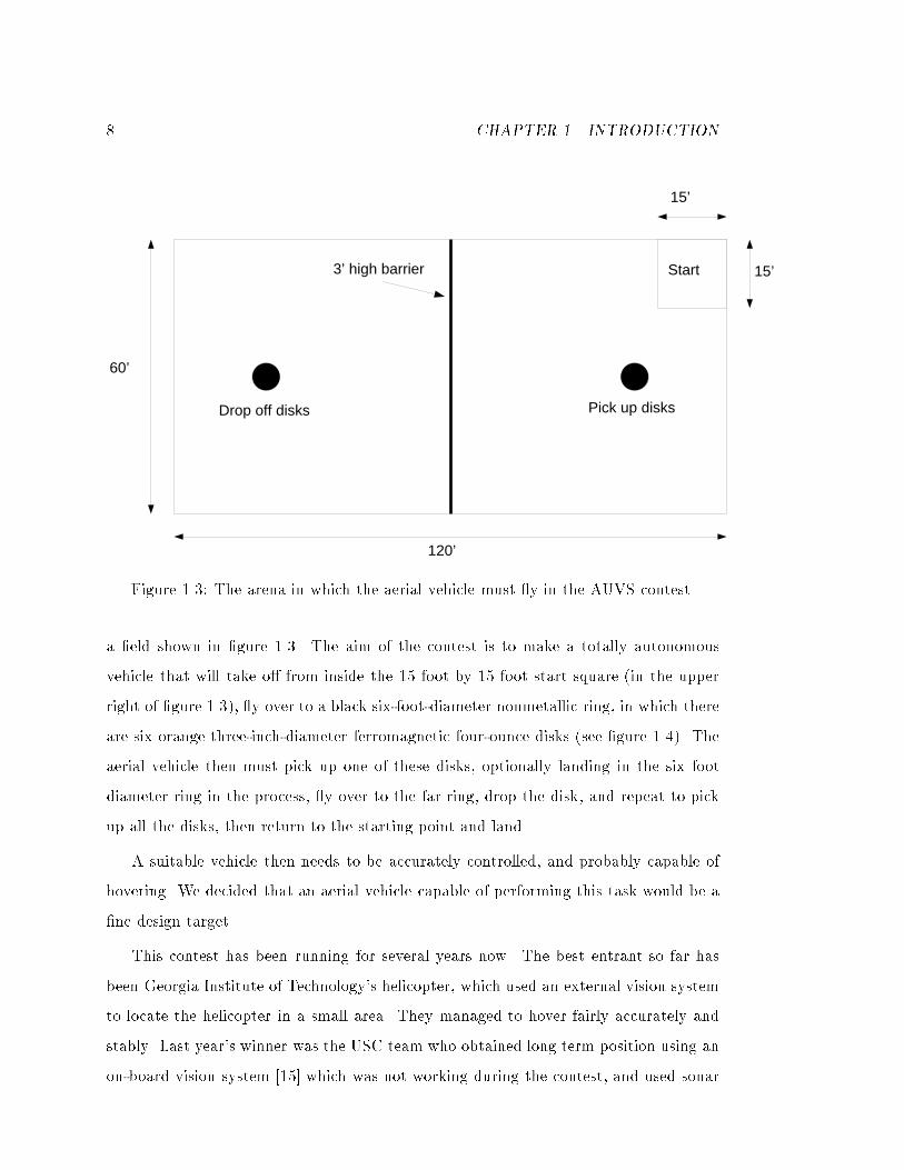
Figure 1.3: The arena in which the aerial vehicle must y in the AUVS contest.
a �eld shown in �gure 1.3. The aim of the contest is to make a totally autonomous
vehicle that will take o� from inside the 15 foot by 15 foot start square (in the upper
right of �gure 1.3), y over to a black six-foot-diameter nonmetallic ring, in which there
are six orange three-inch-diameter ferromagnetic four-ounce disks (see �gure 1.4). The
aerial vehicle then must pick up one of these disks, optionally landing in the six foot
diameter ring in the process, y over to the far ring, drop the disk, and repeat to pick
up all the disks, then return to the starting point and land.
A suitable vehicle then needs to be accurately controlled, and probably capable of
hovering. We decided that an aerial vehicle capable of performing this task would be a
�ne design target.
This contest has been running for several years now. The best entrant so far has
been Georgia Institute of Technology's helicopter, which used an external vision system
to locate the helicopter in a small area. They managed to hover fairly accurately and
stably. Last year's winner was the USC team who obtained long term position using an
on-board vision system [15] which was not working during the contest, and used sonar
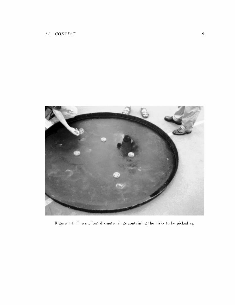
1.5. CONTEST 9
Figure 1.4: The six foot diameter rings containing the disks to be picked up

10 CHAPTER 1. INTRODUCTION
range sensors to obtain altitude, roll and pitch. Another fairly successful team was the
University of Texas at Arlington, who had a tail sitter [6] which used a vision system
(which also did not work at the contest).
We believe that the GPS solution herein is a better long term solution to the sensor
problem in many respects, as it works over a large volume of space, is much easier to set
up, and works in better orientations. GPS has the disadvantage of not working indoors
or in an obstructed environment, but even that is not an insurmountable problem with
pseudolites [24] as mentioned in chapter 6.
1.6 People working on this project
This project was funded by The Boeing Company and The NASA Ames Research Cen-
ter. Professors Robert Cannon and Stephen Rock are the Stanford professors running
the project. I worked full time on this project, being the main organiser, worker and
system integrator. Dr. Steve Morris worked part time as a pilot, helicopter builder,
and control system advisor. Dr. Ben Tigner and Bruce Woodley helped me part time
with various time-consuming parts of the project (it takes a long time to wire up the
connectors needed for this project reliably, etc.). Both Ben and Bruce worked on var-
ious related projects which I have not mentioned in this thesis, as I had little direct
involvement with them, and they are not necessary to the understanding of this project.
Bruce Woodley will be taking over control of the project when I leave. Many other
people have helped in this project as listed in the acknowledgements section, but they
were not formally working on the project.
The work described in the following chapters is my own, or necessary to include for
completeness in order to understand my own.
On the GPS side, the people at the GP-B laboratory gave me advice and aid, but
did generally not work directly with me, with the exception of Paul Montgomery. Paul
is working on a similar aerial vehicle, an airplane. This poses problems that are di�erent
from a helicopter's, in terms of vibration, payload, ight length, other sensors, stability,
wing exure, ability to hover and method of landing. However, very many of our

1.6. PEOPLE WORKING ON THIS PROJECT 11
problems are similar, and he decided to use the programs I had written (see appendices
B and E). In return, he added to the functionality of these programs in several ways:
� He found a few bugs
� He gave me invaluable help with the attitude calculation code, in testing, debug-
ging, and understanding the original problems and hardware.
� He was largely responsible for the velocity calculation work. Paul made the mod-
i�cations to the Trimble TANS units and I did the processing to convert doppler
to velocity.
� He added wing exure and angular velocity code into my attitude code. Whilst I
did not directly use either of these features, they could be useful in the future.
� He was also largely responsible for removing and compressing some of the excess
information that I did not want and which the TANS hardware sent out which
caused increased data lag and decreased sample rate.
Ben Tigner is responsible for a small part of the code in the program
remote.exe which reads the control system gains in from a data �le, and some of the
wiring on the helicopter.
Bruce Woodley is responsible for some of the wiring on the helicopter, and the LEDs
on the tail.
Steve Morris is responsible for all the model helicopter building and ying.
Gad Shelef is responsible for some of the boxes.
Godwin Zhang is responsible for much of the soldering of electronics.
The people at the GP-B laboratory showed me their code. Whilst the implementa-
tion used for the helicopter was written entirely by me (except as explicitly mentioned
above), some of the processing algorithms (part of section 2.3.2) and the linearisation
of the attitude cost function around the current attitude(s) (part of sections 2.3.4 and
2.4.2) are very similar in principle, although the way data is treated and stored was very
di�erent for reasons related to the needs for real-time control, programme maintenance
12 CHAPTER 1. INTRODUCTION
and generality, future growth directions, and the ability to do position/velocity and
attitude/angular velocity simultaneously.
Many people were responsible for the e�ort needed to actually go out, set up the
equipment, and y the helicopter.
Having said that, the following things were my work
� Some key fundamental and generic GPS algorithms
{ Invention and implementation of the `pseudo-global' minimisation algorithm
(sections 2.3.4 and 2.4.2)
{ Invention of the double di�erencing algorithm (section 2.4.1) used for deter-
mining position in automatic control.
{ Some of the new velocity work
{ Some of the work to make the GPS position packets faster.
� Running the project
� Working out the system design
� Implementing almost all the software
{ 68HC11 servo controllers
{ Ground and helicopter based serial drivers
{ GPS algorithms
{ debugging and post-processing aids
{ control software
{ IBM pseudo multitasking work
� Making the servo controller and switch (HC11 board, appendix C.3)
� Lots of little details too small to write up.
� Making sure everything worked simultaneously and together
1.7. OUTLINE OF THESIS 13
1.7 Outline of thesis
Chapter 2 describes how GPS works and the algorithms that are used in processing the
GPS information.
Chapter 3 describes the actual hardware used in this project.
Chapter 4 describes the actual software used in this program, including communica-
tions, diagnostics, implementations of the algorithms in chapter 2, control, and overall
structure.
Chapter 5 describes the experimental ight test results of this project
Chapter 6 describes the new conclusions that can be drawn and gives some ideas for
future work.
This thesis may occasionally contain a few technicalities that are only of interest to
people trying to reproduce or extend some of the engineering in this work rather than
just understand it; I have tried to keep this in the appendices, which are intended to be
used as a reference.
Chapter 2
Global Positioning System
(GPS)
The Global Positioning System is a set of satellites in non-geostationary orbits which
broadcast signals that can be used to determine one's position anywhere on earth with
an accuracy on the order of metres. It was put up by the United States of America's
Department of Defense, in a program run by Bradford Parkinson.
The principle of operation is fairly simple. A receiver on the ground picks up signals
from several satellites. Due to timing information embedded in the signals, the receiver
can determine the time o�set between the local clock in the receiver and the clock on
the satellite. This o�set is the sum of the distance between the satellite and the receiver
and the time error in the local receiver (the time error in the satellite is very small due
to very good and constantly resynchronised clocks). With four or more satellites the
receiver can then solve for the the four variables of position (x,y,z) and local clock o�set
(t).
The details of operation are more complex. The most common method of operation
is to use the C/A (coarse acquisition) signal, which is broadcast from all satellites on
a 1.57542 GHz carrier wave. To distinguish between satellites, a 1.023 MHz pseudo-
random noise (PRN) signal is modulated onto this signal. This signal has a period of
one millisecond, and the 1023 bits for each satellite are chosen to be orthogonal to each
14
15
other in a correlation sense. This means that a receiver can have a bandpass �lter that
picks out the 1.57542 GHz frequency (called L1), down-shifts it to a more manageable
frequency, and then does a correlation with the 1.023 MHz PRN signal for a given
satellite that is expected to be visible. A phase-locked loop then can be used to keep
track of the observed phase of this 1.023 MHz signal. This phase (modulo some number
of milliseconds) then gives the pseudo-range value. Further modulated onto this signal
is a 50 Hz data signal, which contains information for receivers about where satellites
are, what their status is, etc. This, coupled with knowledge of the satellite geometries,
allows a receiver to work out which millisecond is being dealt with, and compute the
position.
A more precise method of ranging, the P-code, is also available. It broadcasts at
a di�erent frequency (L2=1.2276 GHz), and the pseudo-random noise with which each
satellite modulates the carrier is at a ten-times-higher frequency (so phase measurements
are more accurate) and only repeats once a week. Locking on to this signal is rather
di�cult until one has a fairly good idea where one is and what time o�set the receiver
has. This is usually accomplished through the C/A code �rst. Thus a P-code receiver
is about twice as complex as a C/A code receiver.
There are of course various sources of error in the system. The most obvious of
these is how accurately two receivers can measure the phase of the C/A (or P) code
signal. This turns out in practice to be within a few metres for C/A receivers, with
a higher accuracy for P code. Note that from here on this thesis refers to times and
distances interchangeably: assume that the speed of light is equal to one1, so one second
is equivalent to roughly 299,792,458 metres. This is a perfectly valid system of units,
often used in physics. Another major source of errors is the atmosphere, which bends
and slows down radio signals. This leads to errors in the tens of metres. To prevent
undesirables (anyone except the US DoD) from obtaining too high an accuracy for
positioning, whilst still providing a useful service to the commercial world, the US DoD
manipulates the transmitted signals with extra noise known as Selective Availability
(SA) which arti�cially produces further errors in the pseudo-range measurements. This
1One light-second per second.
16 CHAPTER 2. GLOBAL POSITIONING SYSTEM (GPS)
Data Antenna
Base Antenna
Satelite direction s
∆Φ
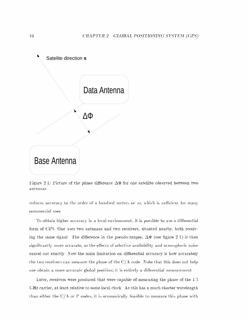
Figure 2.1: Picture of the phase di�erence �� for one satellite observed between twoantennas
reduces accuracy to the order of a hundred metres or so, which is su�cient for many
commercial uses.
To obtain higher accuracy in a local environment, it is possible to use a di�erential
form of GPS. One uses two antennas and two receivers, situated nearby, both receiv-
ing the same signal. The di�erence in the pseudo-ranges, �� (see �gure 2.1) is then
signi�cantly more accurate, as the e�ects of selective availability and atmospheric noise
cancel out exactly. Now the main limitation on di�erential accuracy is how accurately
the two receivers can measure the phase of the C/A code. Note that this does not help
one obtain a more accurate global position; it is entirely a di�erential measurement.
Later, receivers were produced that were capable of measuring the phase of the 1.5
GHz carrier, at least relative to some local clock. As this has a much shorter wavelength
than either the C/A or P codes, it is economically feasible to measure this phase with
17
much higher accuracy in terms of position, and in fact it can be done relatively easily
to give accuracies on the order of millimetres. This has been done for a long time
now; a reasonable description is given in [9]. Basically the carrier is downconverted to
an intermediate frequency of about 4 MHz. An in-phase and quadrature correlation
coe�cient are then measured between this 4 MHz new carrier and the pseudo-random
noise for the particular satellite being tracked, modulated by a reference 4 MHz local
oscillator. A phase-locked loop is then placed around this structure, and the phase is
tracked with updates every millisecond. This in principle means that one could get
di�erential position accuracies with sub centimetre accuracy, which is a very attractive
idea. Such approaches are called carrier phase methods.
However, the way these phases are measured is usually not synchronously with re-
spect to the C/A or P code (as such would be very di�cult), so it is not known in
advance exactly what the phase is in absolute terms: one knows that the phase may
have changed 463.34 cycles since the last measurement, but one does not know exactly
how many cycles there are between two di�erent satellites on the one receiver, or two
di�erent receivers. Once one has determined the o�set between two receivers (the clock
bias, which will not be an integer number of wavelengths), and the integer o�sets be-
tween the satellites on a given receiver, one then has an accurate measurement of ��.
This problem of �nding out these values is known as the Integer resolution problem.
The rest of this chapter deals with how carrier phase measurements are used. In
section 2.3 it is assumed that the integers are known, and the methods of converting
them to useful forms such as position, velocity, attitude and attitude rate are detailed.
In section 2.4 some methods for obtaining these integers are explained. The reason for
this apparently backward order is that the mathematics and algorithms of the integer
resolution methods are more complex than the methods that assume the integers are
known, and they rely on a prior understanding of the simpler algorithms.
18 CHAPTER 2. GLOBAL POSITIONING SYSTEM (GPS)
2.1 Terminology
The following terminology is used throughout the next few sections. It assumes some
number of receivers (usually labeled with superscripts r and s), and various visible
satellites, usually labeled with subscripts i and j.
� c A symbol representing the conversion between the unit seconds and the unit
metres. Not used here as it is unnecessary and clutters up the formulae.
� Xr is quantity X for receiver r
� Xi is quantity X for satellite i
� t is absolute GPS time
� tr is local time for a GPS receiver r.
� �ri (t
r) is the measured phase for satellite i at receiver r relative to the local clock.
� Dri (t
r) is the measured doppler for satellite i at receiver r relative to the local
clock. Dri (t
r) = ddtr
�ri (t
r).
� � r is the time o�set for a particular receiver; tr = t + � r
� xri is the vector distance from satellite i to receiver r
� sri is the unit vector line of sight from receiver r to satellite i. It points towards
the satellites (up in practice).
� �xrs is the 3-displacement of receiver r relative to receiver s.
� �urs is the 3-velocity of receiver r relative to receiver s.
Note that in the following formulae the units involved will not be explicitly men-
tioned. It is assumed that a consistent set of units are used without going into what
they are: distances can be equally well measured in centimetres, metres, inches, sec-
onds or wavelengths. Each is a well de�ned unit of distance with a conversion factor in
between. Using seconds as a distance measurement or metres as a time measurement
2.2. GPS RECEIVER DATA 19
may seem strange | think \light second" instead of second, and think of a second as
just another unit of lenght, with conversion factors left out of formulae in the same way
that conversion factors between inches and miles are left out of formulae2. Cluttering
up formulae with conversion constants adds to the length of already often cumbersome
formulae, and makes the interpretation of relative magnitudes of times and distances
more di�cult. This unit system also makes many quantities dimensionless, which makes
them signi�cantly more easy to work with.
2.2 GPS Receiver data
The GPS receivers used are TANS units, the lower boards from a TANS Quadrex or
Vector. They are manufactured by Trimble and sold to Stanford at a large discount.
They use EPROMs originally programmed at the GP-B laboratory, and last modi�ed
by Paul Montgomery.
The receivers communicate to the external world through a serial line and a packet
protocol (section B.5.1). One sends the receivers various initialisation packets, and
they then automatically send back packets containing phase measurements at 10Hz
together with some other information. This extra information contains some diagnostic
information, plus line-of-sight vectors every thirty seconds or so, which give a unit
vector s pointing to a given satellite for a speci�c time, and also pseudo-range position
information. The pseudo-range position information is the absolute position in space
according to C/A measurements, i.e. conventional GPS. It also gives a fairly accurate
estimate of the local time o�set � , accurate to the order of a hundred metres (roughly
3 � 10�7s).The phase measurements come in one of two forms, depending on the type of
EPROMs used. For position (and velocity) calculations, the GPS board looks at just
one antenna, and measures the phase of the signal from each of up to six visible satellites
relative to the local clock and modulo an integer o�set. It also produces an estimate of
the rate of change of phase. Note that the 10 Hz output rate is precise to the accuracy
2Or in the same way that a physicist may say that an electron may have a mass of 0.5 MeV, implicitlyassuming a division by c2.
20 CHAPTER 2. GLOBAL POSITIONING SYSTEM (GPS)
of the local clock which is about one millisecond. This means that the phase will be
sampled ten times a second, at times up to one millisecond o� the exact GPS time. It
turns out that corrections need to be made for the fact that two di�erent receivers will
produce information at slightly di�erent times.
For attitude, the board looks at four antennas, one of which is designated the master
antenna. The phase and phase rate estimates are then produced for each of up to six
satellites visible for each of the three other antennas relative to the master antenna.
The antennas are linked in a clever multiplexed manner described in detail in [9], so
they all share a common clock, and thus there is only an integer ambiguity and no time
ambiguity as well.
It is possible for one Trimble board to do both, but this was not done in this project
due to the lack of available software to run on the Trimble boards.
2.3 Assume the integers are known
For the moment assume that the integer or time o�sets are known, so that one does not
have to worry about them, and can deal with just the operational solutions that have to
be done in real time with as small phase delay as possible, due to either communication
or computation. To be useful on the helicopter, these computations must execute in a
few milliseconds and not consume excessive memory.
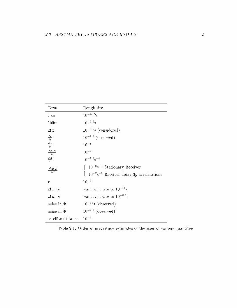
2.3.1 On the Size of quantities
At several times, second-order terms will be neglected in expansions in what follows. To
justify these approximations, it is worthwhile having a close look at the size of various
quantities. These are given in table 2.3.1. Note that for consistency all quantities are
given in units of seconds. A conversion into seconds for a centimetre (level of precision)
and a hundred metres (distance over which the helicopter is expected to operate) are
given.
2.3. ASSUME THE INTEGERS ARE KNOWN 21
Term Rough size
1 cm 10�10:5s
100m 10�6:5s
�x 10�6:5s (considered)
d�dt
10�5:5 (observed)
d�dt
10�5
dx�sdt
10�5
dsdt
10�3:5s�1
d2x�sdt2
8<: 10�8s�1 Stationary Receiver
10�7s�1 Receiver doing 3g accelerations
� 10�3s
�x � s want accurate to 10�11s
�u � s want accurate to 10�9:5s
noise in � 10�11s (observed)
noise in _� 10�9:5 (observed)
satellite distance 10�1s
Table 2.1: Order of magnitude estimates of the sizes of various quantities
22 CHAPTER 2. GLOBAL POSITIONING SYSTEM (GPS)
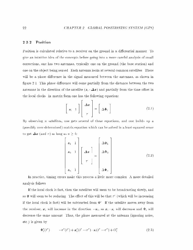
2.3.2 Position
Position is calculated relative to a receiver on the ground in a di�erential manner. To
give an intuitive idea of the concepts before going into a more careful analysis of small
corrections, one has two antennas, typically one on the ground (the base station) and
one on the object being sensed. Each antenna looks at several common satellites. There
will be a phase di�erence in the signal measured between the antennas, as shown in
�gure 2.1. This phase di�erence will come partially from the distance between the two
antennas in the direction of the satellite (si ��x) and partially from the time o�set in
the local clocks. In matrix form one has the following equation:
"si 1
#26664�x
�
37775 =
"��i
#(2:1)
By observing n satellites, one gets several of these equations, and one builds up a
(possibly over-determined) matrix equation which can be solved in a least-squared sense
to get �x (and �) as long as n � 4:266666666666664
s1 1
s2 1
......
sn 1
377777777777775
26664�x
�
37775 =
266666666666664
��1
��2
...
��n
377777777777775
(2:2)
In practice, timing errors make this process a little more complex. A more detailed
analysis follows.
If the local clock is fast, then the satellites will seem to be broadcasting slowly, and
so � will seem to be reducing. The e�ect of this will be that � r (which will be increasing
if the local clock is fast) will be subtracted from �r. If the satellite moves away from
the receiver, xi will increase in the direction �si, so xi � si will decrease and �i will
decrease the same amount. Thus, the phase measured at the antenna (ignoring noise,
etc.) is given by
�ri (t
r) = �� r(tr) + xri (tr � � r) � si(tr � � r) +Ori (2.3)
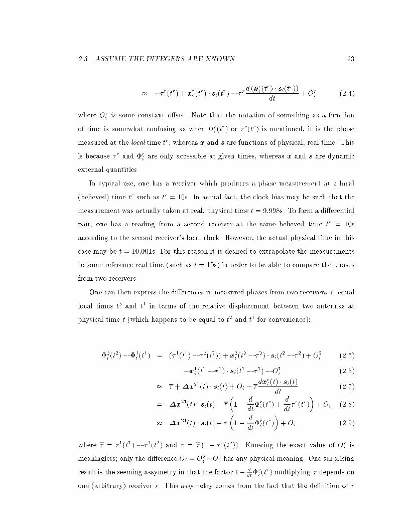
2.3. ASSUME THE INTEGERS ARE KNOWN 23
� �� r(tr) + xri (tr) � si(tr)� � rd (xri (t
r) � si(tr))dt
+Ori (2.4)
where Ori is some constant o�set. Note that the notation of something as a function
of time is somewhat confusing as when �ri (t
r) or � r(tr) is mentioned, it is the phase
measured at the local time tr , whereas x and s are functions of physical, real time. This
is because � r and �ri are only accessible at given times, whereas x and s are dynamic
external quantities.
In typical use, one has a receiver which produces a phase measurement at a local
(believed) time tr such as tr = 10s. In actual fact, the clock bias may be such that the
measurement was actually taken at real, physical time t = 9:998s. To form a di�erential
pair, one has a reading from a second receiver at the same believed time ts = 10s
according to the second receiver's local clock. However, the actual physical time in this
case may be t = 10:001s. For this reason it is desired to extrapolate the measurements
to some reference real time (such as t = 10s) in order to be able to compare the phases
from two receivers.
One can then express the di�erences in measured phases from two receivers at equal
local times t2 and t1 in terms of the relative displacement between two antennas at
physical time t (which happens to be equal to t2 and t1 for convenience):
�2i (t
2)� �1i (t
1) = (�1(t1)� �2(t2)) + x2i (t2 � �2) � si(t2 � �2) + O2i (2.5)
�x1i (t1 � �1) � si(t1 � �1)�O1i (2.6)
� � +�x21(t) � si(t) + Oi + �dxri (t) � si(t)
dt(2.7)
= �x21(t) � si(t) + �
�1 +
d
dt�ri (t
r) +d
dt� r(tr)
�+ Oi (2.8)
� �x21(t) � si(t) + �
�1 +
d
dt�ri (t
r)
�+Oi (2.9)
where � = �1(t1) � �2(t2) and � = � (1 + _� r(tr)). Knowing the exact value of Ori is
meaningless; only the di�erence Oi = O2i �O1
i has any physical meaning. One surprising
result is the seeming assymetry in that the factor 1+ ddt�ri (t
r) multiplying � depends on
one (arbitrary) receiver r. This assymetry comes from the fact that the de�nition of �
24 CHAPTER 2. GLOBAL POSITIONING SYSTEM (GPS)
is also slightly assymetric, and these two assymetries cancel out to the level of precision
relevent here.
This now gives a set of equations similar to the na��ve equation (2.2), which can be
again solved in a least-squared sense with very little extra e�ort:266666666666664
s1 1 + ddt�r1(t
r)
s2 1 + ddt�r2(t
r)
......
sn 1 + ddt�rn(t
r)
377777777777775
26664�x21
�
37775 =
266666666666664
�21(t
2)� �11(t
1)� O1
�22(t
2)� �12(t
1)� O2
...
�2n(t
2)� �1n(t
1)� On
377777777777775
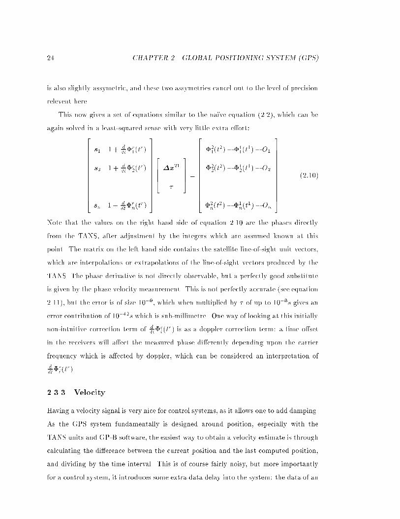
(2:10)
Note that the values on the right hand side of equation 2.10 are the phases directly
from the TANS, after adjustment by the integers which are assumed known at this
point. The matrix on the left hand side contains the satellite line-of-sight unit vectors,
which are interpolations or extrapolations of the line-of-sight vectors produced by the
TANS. The phase derivative is not directly observable, but a perfectly good substitute
is given by the phase velocity measurement. This is not perfectly accurate (see equation
2.11), but the error is of size 10�9, which when multiplied by � of up to 10�3s gives an
error contribution of 10�12s which is sub-millimetre. One way of looking at this initially
non-intuitive correction term of ddt�ri (t
r) is as a doppler correction term: a time o�set
in the receivers will a�ect the measured phase di�erently depending upon the carrier
frequency which is a�ected by doppler, which can be considered an interpretation of
ddt�ri (t
r).
2.3.3 Velocity
Having a velocity signal is very nice for control systems, as it allows one to add damping.
As the GPS system fundamentally is designed around position, especially with the
TANS units and GP-B software, the easiest way to obtain a velocity estimate is through
calculating the di�erence between the current position and the last computed position,
and dividing by the time interval. This is of course fairly noisy, but more importantly
for a control system, it introduces some extra data delay into the system: the data of an
2.3. ASSUME THE INTEGERS ARE KNOWN 25
extra sample ago (a tenth of a second) is being used in the current estimate of velocity.
Filters can reduce the e�ect of the noise, but that tends to increase the data delay still
further. This is very bad for control: data delay can easily mean the di�erence between
instability and stability.
The GPS receivers measure phase directly; that is the fundamental measurement.
But internally, they contain a �lter that maintains an estimate of the phase velocity at
the local update rate that is typically much higher than the rate at which the phase
data is sent over the serial port. For the TANS units used on the helicopter, the internal
update rate is more than an order of magnitude higher update rate than the output
rate of 10Hz. In principle it could be signi�cantly higher. This means that the delay
in the measured velocity signal could be less if it were computed using these data.
Paul Montgomery (with some help from me) modi�ed the TANS software to emit these
phase velocities with precision of 0:03Hz (six millimetres per second). The noise tended
to be a bit under one hertz upon experimentation, which is comparable to the noise in
�rst-di�erence estimates.
The signal produced Dri is the derivative of the measured phase of satellite i with
respect to the local clock in receiver r. Again, as for position, the di�erence between
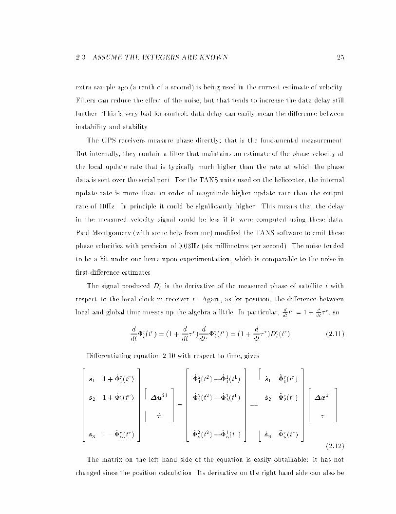
local and global time messes up the algebra a little. In particular, ddttr = 1+ d
dt� r, so
d
dt�ri (t
r) = (1 +d
dt� r)
d
dtr�ri (t
r) = (1 +d
dt� r)Dr
i (tr) (2:11)
Di�erentiating equation 2.10 with respect to time, gives
266666666666664
s1 1 + _�r1(t
r)
s2 1 + _�r2(t
r)
......
sn 1 + _�rn(t
r)
377777777777775
26664�u21
_�
37775 =
266666666666664
_�21(t
2)� _�11(t
1)
_�22(t
2)� _�12(t
1)
...
_�2n(t
2)� _�1n(t
1)
377777777777775�
266666666666664
_s1 ��r1(t
r)
_s2 ��r2(t
r)
......
_sn ��rn(t
r)
377777777777775
26664�x21
�
37775
(2:12)
The matrix on the left hand side of the equation is easily obtainable: it has not
changed since the position calculation. Its derivative on the right hand side can also be

26 CHAPTER 2. GLOBAL POSITIONING SYSTEM (GPS)
calculated relatively straightforwardly, as they contribute only a very small correction
term to the velocity calculation. The rate of change of line of sights is easy | if one
can interpolate, one can get a reasonable time rate of change. The second derivative of
phase comes from �rst di�erences of D. Again, this term is so tiny that the di�erences
between D and _� are insigni�cant. The position and time o�set come from the position
calculation, which should be done just before the velocity calculation.
This just leaves the phase derivatives to be calculated. Unfortunately, the local clock
issue means that one cannot quite just say _� = D. Firstly, note that to �rst order
D2i �D1
i = (1� _�2)�_�2 � _�1
�+ _� _�1 (2.13)
= (1� _�1)�_�2 � _�1
�+ _� _�2 (2.14)
so that one may update this equation to
266666666666664
s1 1 + 2 _�r1(t
r)
s2 1 + 2 _�r2(t
r)
......
sn 1 + 2 _�rn(t
r)
377777777777775
26664�u21
_�
37775 =
1
1� _� s
266666666666664
D21(t
2)�D11(t
1)
D22(t
2)�D12(t
1)
...
D2n(t
2)�D1n(t
1)
377777777777775�
266666666666664
_s1 ��r1(t
r)
_s2 ��r2(t
r)
......
_sn ��rn(t
r)
377777777777775
26664�x21
�
37775
(2:15)
where s and r represent the two receivers (in either order).
In practice, with the current receivers used on the helicopter, it is perfectly �ne to
ignore the factor of 1=(1� _� s), as the correction terms from the position calculation are
small, so the net result will be to just overestimate the velocity by a factor of 1 � _� s,
which is tiny compared to the noise for anything subsonic. The value of _� can be
obtained fairly easily from di�erencing the clock-bias information in the pseudo-range
position packets from the TANS.
In practice, it is also �ne to ignore the factor of 2 which appeared in the leftmost
matrix in equation 2.15, as the term it multiplies also has a small e�ect with the current
level of noise. This seemingly pointless approximation is mentioned here since there
exist signi�cant intermediate computations (the Cholsky factorisation of the matrix in
2.3. ASSUME THE INTEGERS ARE KNOWN 27
question) from the position calculation step that can be reused saving execution time if
the leftmost matrix in equations 2.10 and 2.15 are the same.
2.3.4 Attitude
Given the relative position of antennas to the order of a centimetre, it is possible to
use GPS information to determine attitude (suggested in [21] with real time work in
eg. [12, 11, 9, 19, 17]). Clearly at least three antennas are needed, and having more
antennas will help increase robustness through data redundancy. Cohen [9] obtained
attitude using a carrier phase receiver with multiplexed inputs. One receiver would
then look at each of the four antennas in turn, and would measure the phase di�erence
between each antenna and some master antenna. This has the advantage over other
similar approaches with multiple receivers of avoiding the time di�erence between the
local clocks in the receiver, and probably being cheaper to manufacture. There is a
disadvantage in that high unexpected accelerations can cause cycle slips if the vehicle
moves too far unexpectedly in the time period when the moving antenna is disconnected,
but this is not a problem for movements likely on a helicopter.
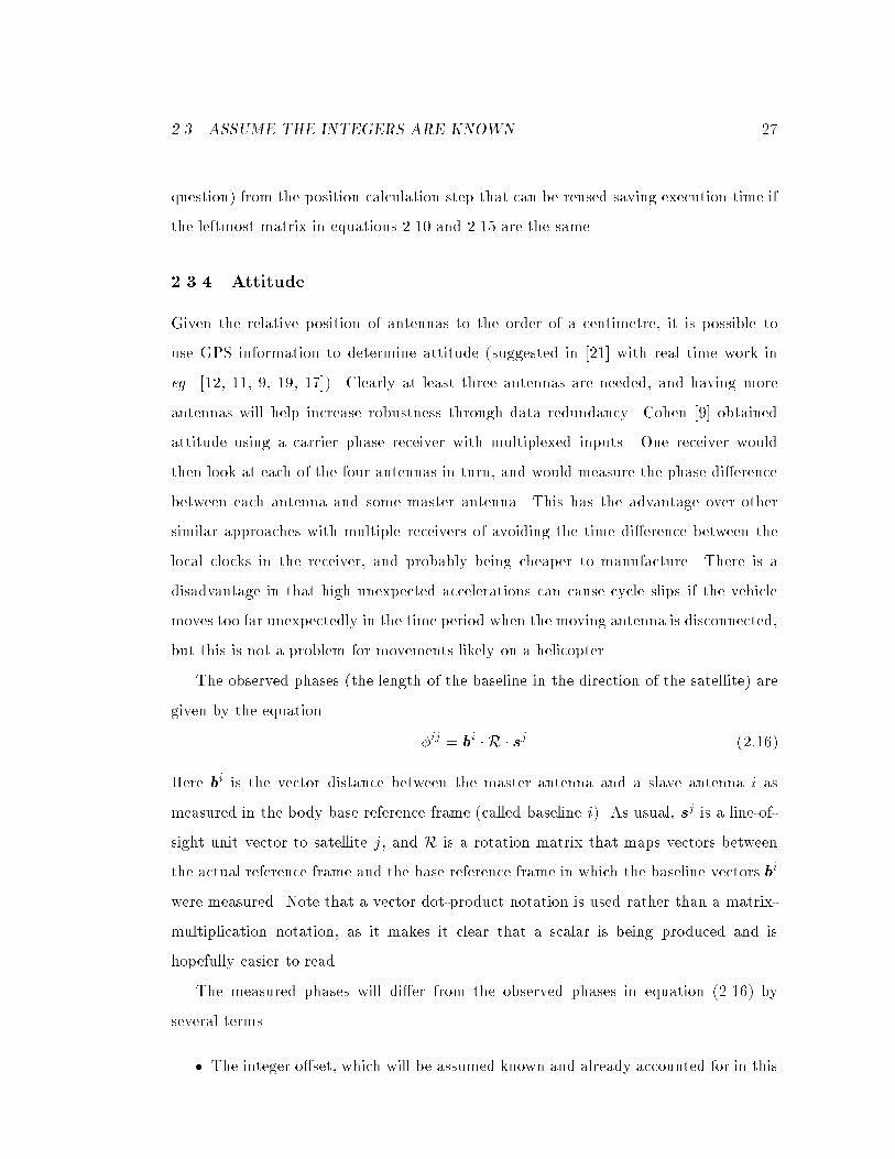
The observed phases (the length of the baseline in the direction of the satellite) are
given by the equation
�ij = bi � R � sj (2:16)
Here bi is the vector distance between the master antenna and a slave antenna i as
measured in the body base reference frame (called baseline i). As usual, sj is a line-of-
sight unit vector to satellite j, and R is a rotation matrix that maps vectors between
the actual reference frame and the base reference frame in which the baseline vectors bi
were measured. Note that a vector dot-product notation is used rather than a matrix-
multiplication notation, as it makes it clear that a scalar is being produced and is
hopefully easier to read.
The measured phases will di�er from the observed phases in equation (2.16) by
several terms
� The integer o�set, which will be assumed known and already accounted for in this
28 CHAPTER 2. GLOBAL POSITIONING SYSTEM (GPS)
section
� The line bias (phase di�erence due to the di�ering lengths of antenna cables). This
can be calibrated in advance and accounted for by subtraction from the measured
phase. All future measured phases will be assumed to have had this calibrated
value subtracted from them already.
� Noise
To calculate the attitude (represented by the rotation matrix R), given several phasemeasurements, one wishes to solve a set of equations like equation (2.16). As R can
be considered to be speci�ed by three independent parameters, one needs at least three
phases. In practice, there tend to be signi�cantly more than three available, and one
solves this equation in a least-squared sense. Thus one wants to �nd a R that minimises
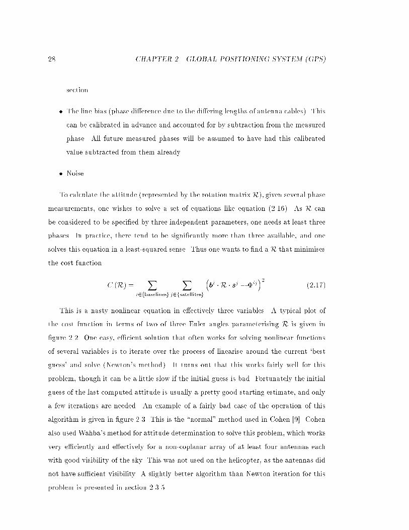
the cost function
C (R) =X
i2fbaselinesg
Xj2fsatellitesg
�bi � R � sj � �ij
�2(2:17)
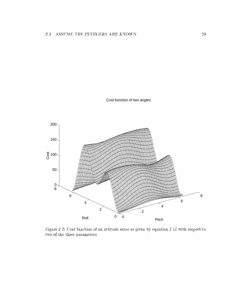
This is a nasty nonlinear equation in e�ectively three variables. A typical plot of
the cost function in terms of two of three Euler angles parameterising R is given in
�gure 2.2. One easy, e�cient solution that often works for solving nonlinear functions
of several variables is to iterate over the process of linearise around the current `best
guess' and solve (Newton's method). It turns out that this works fairly well for this
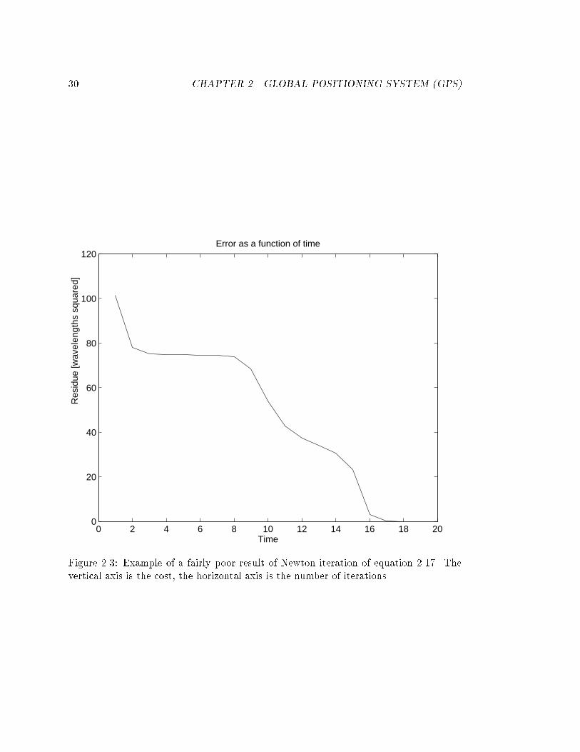
problem, though it can be a little slow if the initial guess is bad. Fortunately the initial
guess of the last computed attitude is usually a pretty good starting estimate, and only
a few iterations are needed. An example of a fairly bad case of the operation of this
algorithm is given in �gure 2.3. This is the \normal" method used in Cohen [9]. Cohen
also used Wahba's method for attitude determination to solve this problem, which works
very e�ciently and e�ectively for a non-coplanar array of at least four antennas each
with good visibility of the sky. This was not used on the helicopter, as the antennas did
not have su�cient visibility. A slightly better algorithm than Newton iteration for this
problem is presented in section 2.3.5.
2.3. ASSUME THE INTEGERS ARE KNOWN 29
02
46
8
0
2
4
6
80
50
100
150
200
PitchRoll
Cos
t
Cost function of two angles
Figure 2.2: Cost function of an attitude error as given by equation 2.17 with respect totwo of the three parameters.
30 CHAPTER 2. GLOBAL POSITIONING SYSTEM (GPS)
0 2 4 6 8 10 12 14 16 18 200
20
40
60
80
100
120Error as a function of time
Time
Res
idue
[wav
elen
gths
squ
ared
]
Figure 2.3: Example of a fairly poor result of Newton iteration of equation 2.17. Thevertical axis is the cost, the horizontal axis is the number of iterations.
2.3. ASSUME THE INTEGERS ARE KNOWN 31
Note that the baselines and the line biases can be obtained through a self survey
over a period of several hours [9].
2.3.5 Pseudo-global attitude solution
For reasons which will become clear in section 2.4.2 the linearise-and-solve method used
in section 2.3.4 was not entirely satisfactory to solve equation 2.17. It would be useful
to have an approach that converged more rapidly in cases when the initial guess was
very bad. The following section describes an algorithm that works well for bad initial
guesses.
Consider an estimate of attitude R. Consider the problem of �nding the best value
of such that the new rotation matrix R0 de�ned by
R0 =
2666666664
cos sin 0
� sin cos 0
0 0 1
3777777775R (2:18)
has the smallest cost function.
C (R;) =X
i2fbaselinesgj2fsatellitesg
0BBBBBBBB@bi �
2666666664
cos sin 0
� sin cos 0
0 0 1
3777777775R � sj � �ij
1CCCCCCCCA
2
(2.19)
=X
i2fbaselinesgj2fsatellitesg
(a1 cos + a2 sin + a3)2 (2.20)
= c1 cos2+ c2 sin
2+ c3 cos sin + c4 cos + c5 sin + c6(2.21)
= d1 cos(2 + �1) + d2 cos( + �2) + d3 (2.22)
where ai, ci, di, and �i are numbers that can be readily and e�ciently calculated for
given R, phases �ij , baselines bi and line-of-sight unit vectors sj . One wants to �nd
a value of that minimises this. So one wants to �nd the minimum of d1 cos(2 +
�1) + d2 cos( + �2) as d3 is irrelevant to the minimisation. Without loss of generality
32 CHAPTER 2. GLOBAL POSITIONING SYSTEM (GPS)
accomplished via manipulations of �1 and �2, assume that d1 � 0 and d2 � 0. Divide3
through by d1, and make the substitution x = + 12�1, B = d2=d1 � 0 and � = �2� 1
2�1.
Then one wants to �nd x to minimise
C(x) = cos 2x+ B cos(x+ �): (2:23)
Actually �nding the minimum of this equation can be done e�ciently computationally;
a description of the algorithm is given in section 2.3.6. Given a value of x, one can
apply the above simpli�cations backwards to obtain an optimal value of to minimise
equation (2.19). This can then be used to modify the current attitude estimate.
One then repeats this process for rotations around the other two axes, mutatis
mutandis, and this makes up a single iteration of my pseudo-global iteration algorithm.
An iteration of this algorithm is generally better than the normal linearise-and-
solve method (Newton's method) when the estimate is far from the true value, as it
can jump over ridges as are evident in �gure 2.2, whereas Newton's method provides
quadratic convergence near the true value and is thus superior for later steps of iteration.
For this reason, in practice, two iterations of this global algorithm followed by Newton's
algorithm until the value of the cost function stops decreasing, works very well, typically
taking one to two Newton iterations.
In practice this is not a large improvement here: Newton's algorithm does work
adequately for this problem. The reason for introducing this algorithm is it's value for
solving a more complex cost function, as appears in section 2.4.2.
2.3.6 Finding the minimum of equation 2.23
One knows that B � 0 from the way B is determined in practice4; and one can clearly
assume that � is between 0 and 2�. If � > � one can make the transformations x! �xand �! 2��� and one ends up solving the same equation form except with � between
0 and �, so one can assume without loss of generality that 0 � � � �. Furthermore, if
3If d1 is near zero, and d2 is not, then the solution is trivial. If both are near zero, then the result isnot important anyway as has no real e�ect on the cost
4In any case one could change the sign of B via adding � to �.
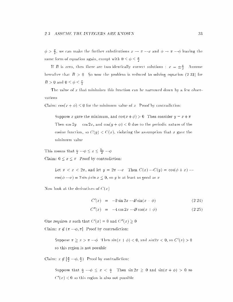
2.3. ASSUME THE INTEGERS ARE KNOWN 33
� > �2 , we can make the further substitutions x ! � � x and � ! � � � leaving the
same form of equation again, except with 0 � � � �2 .
If B is zero, then there are two identically correct solutions : x = ��2 . Assume
hereafter that B > 0. So now the problem is reduced to solving equation (2.23) for
B > 0 and 0 � � � �2 .
The value of x that minimises this function can be narrowed down by a few obser-
vations.
Claim: cos(x+ �) � 0 for the minimum value of x. Proof by contradiction:
Suppose x gave the minimum, and cos(x+�) > 0. Then consider y = x+�.
Then cos 2y = cos 2x, and cos(y + �) < 0 due to the periodic nature of the
cosine function, so C(y) < C(x), violating the assumption that x gave the
minimum value.
This means that �2 � � � x � 3�
2 � �.Claim: 0 � x � �. Proof by contradiction:
Let � < x < 2�, and let y = 2� � x. Then C(x) � C(y) = cos(� + x) �cos(�� x) = 2 sin� sin x � 0, so y is at least as good as x.
Now look at the derivatives of C(x).
C 0(x) = �2 sin 2x�B sin(x+ �) (2.24)
C00(x) = �4 cos 2x�B cos(x+ �) (2.25)
One requires x such that C0(x) = 0 and C00(x) � 0.
Claim: x 62 (� � �; �]. Proof by contradiction:
Suppose � � x > � � �. Then sin(x+ �) < 0, and sin2x < 0, so C0(x) > 0
so this region is not possible.
Claim: x 62 [�2 � �; �2 ). Proof by contradiction:
Suppose that �2 � � � x < �
2 . Then sin 2x � 0 and sin(x + �) > 0 so
C0(x) < 0 so this region is also not possible.
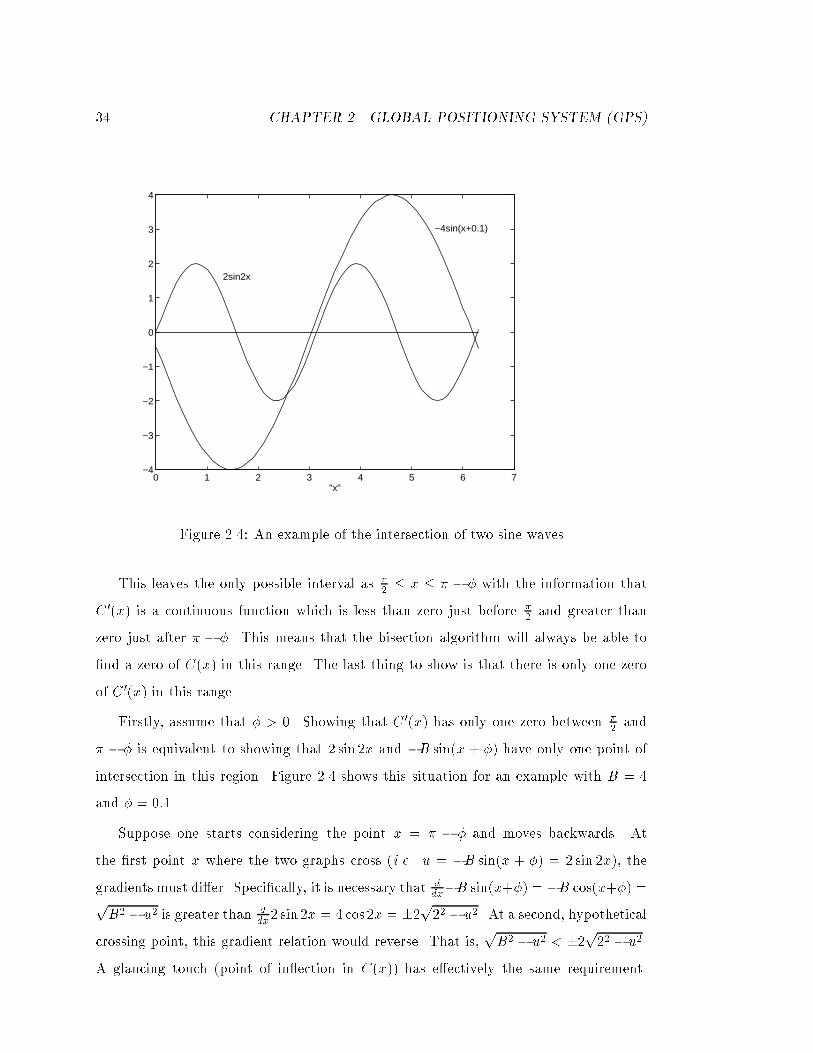
34 CHAPTER 2. GLOBAL POSITIONING SYSTEM (GPS)
0 1 2 3 4 5 6 7−4
−3
−2
−1
0
1
2
3
4
"x"
2sin2x
−4sin(x+0.1)
Figure 2.4: An example of the intersection of two sine waves
This leaves the only possible interval as �2 � x � � � � with the information that
C0(x) is a continuous function which is less than zero just before �2 and greater than
zero just after � � �. This means that the bisection algorithm will always be able to
�nd a zero of C(x) in this range. The last thing to show is that there is only one zero
of C0(x) in this range.
Firstly, assume that � > 0. Showing that C0(x) has only one zero between �2 and
� � � is equivalent to showing that 2 sin 2x and �B sin(x + �) have only one point of
intersection in this region. Figure 2.4 shows this situation for an example with B = 4
and � = 0:1.
Suppose one starts considering the point x = � � � and moves backwards. At
the �rst point x where the two graphs cross (i.e. u = �B sin(x + �) = 2 sin 2x), the
gradients must di�er. Speci�cally, it is necessary that ddx�B sin(x+�) = �B cos(x+�) =
pB2 � u2 is greater than d
dx2 sin 2x = 4 cos2x = �2p22 � u2. At a second, hypothetical
crossing point, this gradient relation would reverse. That is,pB2 � u2 < �2p22 � u2.
A glancing touch (point of in ection in C(x)) has e�ectively the same requirement.
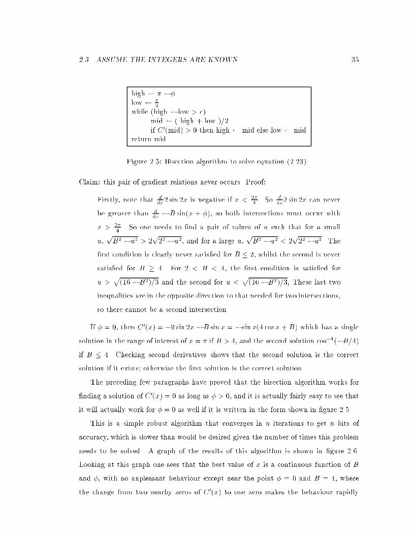
2.3. ASSUME THE INTEGERS ARE KNOWN 35
high � � �low �
2while (high � low > �)
mid ( high + low )=2if C0(mid) > 0 then high mid else low mid
return mid
Figure 2.5: Bisection algorithm to solve equation (2.23).
Claim: this pair of gradient relations never occurs. Proof:
Firstly, note that ddx2 sin 2x is negative if x < 3�
4 . So ddx2 sin 2x can never
be greater than ddx� B sin(x + �), so both intersections must occur with
x > 3�4 . So one needs to �nd a pair of values of u such that for a small
u,pB2 � u2 > 2
p22 � u2, and for a large u,
pB2 � u2 < 2
p22 � u2. The
�rst condition is clearly never satis�ed for B � 2, whilst the second is never
satis�ed for B � 4. For 2 < B < 4, the �rst condition is satis�ed for
u >p(16�B2)=3 and the second for u <
p(16� B2)=3, These last two
inequalities are in the opposite direction to that needed for two intersections,
so there cannot be a second intersection.
If � = 0, then C0(x) = �2 sin 2x� B sin x = � sin x(4 cosx+ B) which has a single
solution in the range of interest of x = � if B > 4, and the second solution cos�1(�B=4)if B � 4. Checking second derivatives shows that the second solution is the correct
solution if it exists; otherwise the �rst solution is the correct solution.
The preceding few paragraphs have proved that the bisection algorithm works for
�nding a solution of C0(x) = 0 as long as � > 0, and it is actually fairly easy to see that
it will actually work for � = 0 as well if it is written in the form shown in �gure 2.5.
This is a simple robust algorithm that converges in n iterations to get n bits of
accuracy, which is slower than would be desired given the number of times this problem
needs to be solved. A graph of the results of this algorithm is shown in �gure 2.6.
Looking at this graph one sees that the best value of x is a continuous function of B
and �, with no unpleasant behaviour except near the point � = 0 and B = 4, where
the change from two nearby zeros of C0(x) to one zero makes the behaviour rapidly

36 CHAPTER 2. GLOBAL POSITIONING SYSTEM (GPS)
00.5
11.5
2
0
5
10
15
201.5
2
2.5
3
3.5
φB
x
Minimum x in cos 2x + B cos(x+φ)
Figure 2.6: A graph of x giving the minimum of cos 2x+ B cos(x+ �) as a function ofB and �.
changing and non-di�erentiable though still continuous. Indeed, except near this point
(with multiple nearby zeros of C0(x)) it can be shown that Newton iteration works very
well, given a su�ciently close initial estimate. For a smooth function like this, a small
2-D table lookup with interpolation works adequately and e�ciently as an initial guess.
For the purposes of a lookup table, the in�nite range of B can be mapped into a �nite
range through an index function like B=(1 + B), as the estimates do not change much
as B approaches in�nity.
In the actual implementation, the algorithm �rstly checks to see if the values of B
and � were close to B = 4 and � = 0. If they were very close, the algorithm uses
the bisection algorithm which is guaranteed to work, although it will not converge as
quickly as Newton iteration. If they were fairly close, the algorithm uses a small local
2.3. ASSUME THE INTEGERS ARE KNOWN 37
0
0.2
0.4
0.6
0.8
1
1.2
1.4
1.6
0 5 10 15 20 25 30 35 40
φ
B
Figure 2.7: A scatter plot of the values of B and � for which the minimum of equation2.23 was needed during a typical ight.
table lookup followed by Newton iteration; if they were not close to the trouble spot
a more coarse table lookup and then Newton iteration is used. With this arrangement
only one or two Newton iterations were required for about �ve digits accuracy in x.
Note that the Newton iteration mentioned here is only in one variable, and consists
of a dozen odd operations; it is not nearly as computationally expensive as a multidi-
mensional Newton iteration.
The purpose of the two separate tables is to conserve memory by not having a �ne
lookup table were it not needed. An equivalent alternative to the two tables would be
a complex index function of B and � expanding the phase space near B = 4, � = 0.
A scatter-graph of the values of B and � sent to this algorithm during a typical
ight is shown in �gure 2.7 This demonstrates that in practice, the values of B and �
are not particularly congregated around B = 4 and � = 0; so the average e�ciency of
this approach is very high, since the bisection algorithm is rarely resorted to.
38 CHAPTER 2. GLOBAL POSITIONING SYSTEM (GPS)
In summary, it is possible to �nd the minimum of equation (2.23) in a computation-
ally e�cient manner.
2.3.7 Attitude Rate
In a similar manner to velocity, Paul Montgomery et al. [18] obtained attitude rate
signals. This involves a computationally simple step after the attitude calculation. It
is mentioned here for completeness, as it can be and is measured and calculated on the
helicopter. Details are not presented here as this implementation was done by Paul,
and is not signi�cantly di�erent from [18]. This signal was not used for control on the
helicopter for several reasons which will be discussed in section 4.4.
2.4 Obtaining Integers
So far this discussion has assumed that the integer o�sets were known. As the phase
integrity is maintained once the phase-locked loop has locked onto the signal, the integers
have only to be determined once. There are several ways to obtain the integers.
Firstly, one can just declare the integers by �at. If one knows the relative position
of the antennas accurately, one can get su�ciently accurate time bias information from
the pseudo-range packets, and then say \This is your position; calculate the integers
from that." This has the disadvantage of requiring the initial o�sets to be known as
accurately as possible5 (which is actually easy to do on the ground with the antennas in
a known position). For the attitude integers, this would involve putting the helicopter
in a known attitude. For the position integers, this would mean putting the helicopter
and base station in a known relationship. Even if the initial position is out by a few
metres, this is unlikely to be a disaster, as the drift rate it would introduce from satellite
motion would be fairly low. Another problem is that the imputed integers when new
satellites arrive would not lie close to integer boundaries, so a drift could come from
there. Still, we have had considerable success with this approach with the helicopter for
position.
5Preferably within half a wavelength, though search algorithms can be used to increase this limit
2.4. OBTAINING INTEGERS 39
Secondly, one can use a searching algorithm. If one knows limits on the integers
(easy to get directly for the attitude integers, and by using di�erential GPS for a rough
estimate of the position integers). This has the disadvantages of being slow and often
inconclusive.
Another method is by geometry change. If the geometry of the baseline (the vector
distance between two antennas) relative to the satellites' line of sight vectors changes,
then the way the phases change over time can give su�cient information to resolve
the integers. There are two di�erent approaches commonly used: change the baseline
quickly (with the satellites remaining roughly stationary) or hold the baseline constant
with the satellites moving. The former is used when the baseline is short and can be
changed in a controlled manner, such as when the antennas are mounted on a rigid body
and their scalar separations are �xed. This was the chosen method for determining the
attitude integers. The latter method, of waiting for satellite motion, has been used
extensively by surveyors who put down two receivers and wait. This method is not
particularly ideal for automatic control as it involves a lengthy wait before starting.
A variation on these methods is to mount a pseudolite (basically an equivalent of
the transmitting portion of a satellite) on the ground, and have an airplane y over,
observing the phases from both the satellites above and the pseudolite below [8]. This
is truly perfect for airplanes coming in to land at an airport | the integers relative to
a receiver on the runway can be computed as the airplane lands { but it is not ideal for
an autonomous helicopter for several reasons. There are all sorts of pragmatic reasons
about mounting of antennas and pseudolites in the �eld, but also it means that the
helicopter has to y a signi�cant distance before it can resolve the integers. This is not
really possible for a supposedly fully autonomous vehicle, although there are possible
methods of �nessing this problem. Anyway, avoiding having to use a pseudolite to
resolve the position integers would make the helicopter signi�cantly more useful. More
useful still, of course, is to have pseudolites around that both add information (replacing
poorly seen satellites) and provide useful geometrical information for resolving integers.
Having the option of both is of course the best.
In practice at present, the motion method is used for attitude, and an initial-guess

40 CHAPTER 2. GLOBAL POSITIONING SYSTEM (GPS)
method is used for the position. A time-based guess re�nement method described in
section 2.4.1 can be used to o�set problems due to drifting position. These solutions
will now be described in more detail.
2.4.1 Position
Suppose that one did not know the exact integers for a position o�set, but instead just
obtained some that were fairly close. As mentioned previously, this can be done by
obtaining the time biases from the GPS pseudo-range packets, and relative positions
can be obtained through regular di�erential GPS, or by just assuming that the two
antennas start o� close, so that the distance can be approximated to zero.
This section will need a more compact notation than previously as it will now be
dealing with many measurements, and it will not need to go into as much detail on each
individual measurement. One can now rewrite equation 2.10 in the form StXt = �t
where St is now a whole matrix of antenna line-of-sight vectors and doppler corrections,
X t is a four vector of position and time o�set, and �t is a vector of all the phases
known. The t now denotes the measurements at some particular time.
Suppose that the integers were o� by some o�set C, so that the true value of X t is
actually given by the equation
StXt +C = �t (2:26)
The immediate e�ect that this would have on the computed position X t is an error of
S�1t C (where the matrix inverse is taken to mean solution in a least squared sense if Stis not square).
The next question is \What does this error mean?" There are two answers. The
obvious answer is that it is the error in the computed position from the base station.
For a surveyor, this would be the error in the measurement | a bad thing. For an
airplane coming in to land, assuming the base station is at a �xed position relative to
the runway, this is the error in the distance to the ground | also a bad thing. For an
autonomous helicopter, this is the error in the position of the base station | which is
not necessarily a bad thing. If the helicopter is trying to hover, for instance, it does not
2.4. OBTAINING INTEGERS 41
matter whether it knows exactly where it is relative to the base station | it only cares
about its distance relative to where it is trying to hover, and if that was calculated via
the same process with the same error, then these errors cancel out and it is irrelevant.
For this reason, there are a lot of tasks that an autonomous vehicle can do without
knowing the integers exactly.
The trouble comes as the time span gets greater. Although C is time independent,
S�1t is not, as the satellites are moving. This messes up the whole situation as the
relative error from previous positions will be�S�1t2� S�1t1
�C, which will grow as t2 and
t1 get further apart. However, by this stage there has been some signi�cant satellite
movement by de�nition, and one can use the surveyors' method of resolving integers
through satellite motion.
The method about to be described is based on the ideas outlined above. For early
time, the satellites have not moved much, and it is a reasonable assumption that the
relative error due to incorrect integers is small. As the satellites move more, one builds
up an estimate of C and uses it to make corrections, preventing the error from ever
getting too large. Using this algorithm, very little e�ort is required to initialise the
helicopter: one just takes it out to where one wants to y, puts the base antenna
somewhere nearby, it does not matter much where, maybe turns the helicopter around
to initialise the attitude integers, and then it is ready to go. It doesn't know the integers
exactly yet, but it does not need them immediately. This would save considerable e�ort
by the ground sta� over other approaches, and in particular makes the helicopter much
more usable for applications such as power line inspection in remote areas without a
pseudolite mounted in a handy position.
Since this algorithm relies on satellites beyond the four minimum to determine po-
sition, it is very helpful to have more than six satellites visible. For this reason, a GPS
receiver with more channels than the Trimble TANS may be useful.
Algorithm
This algorithm is similar in many regards to proposals for on-the- y kinematic position-
ing [16, 14], which di�er from the normal surveying technique of putting down antennas
42 CHAPTER 2. GLOBAL POSITIONING SYSTEM (GPS)
and waiting for the satellites to move by allowing one antenna to move. The di�erences
with this approach are
� The emphasis on real-time implementability
� The ability to deal with changing satellites or temporary outages leading to cycle
slips in a poor-visibility environment
� Dealing with doppler corrections in the time o�set between receivers
� Most importantly, the overall philosophy of producing instantly usable position
data that can be e�ciently updated later in real time.
If one has four satellites and a moving vehicle, there is not much one can do. But
with more than four satellites, one has redundant information which can be used to get
the estimate for C.
Collecting equation 2.26 over time gives the following matrix equation:
266666666666664
S1 0 � � � 0 I
0 S2 � � � 0 I...
0 0 � � � Sn I
377777777777775
2666666666666666664
�X1
�X2
...
�Xn
C
3777777777777777775
=
266666666666664
�1
�2
...
�n
377777777777775
(2:27)
If one actually tries to solve this equation, one �nds that there is a vector that comes
very close to being in the null space of the matrix on the left hand side of equation (2.27).
This vector corresponds to all the integers being increased by a constant amount �, and
all the time biases being decreased by the same amount. As the integers trying to be
determined in equation 2.27 are typically small, being just the residues after a fairly
good approximation with conventional GPS, the e�ects due to the doppler corrections
will be tiny, causing it to be unreasonable and pointless to try to distinguish between
o�sets in all the integers or all the receiver time errors.
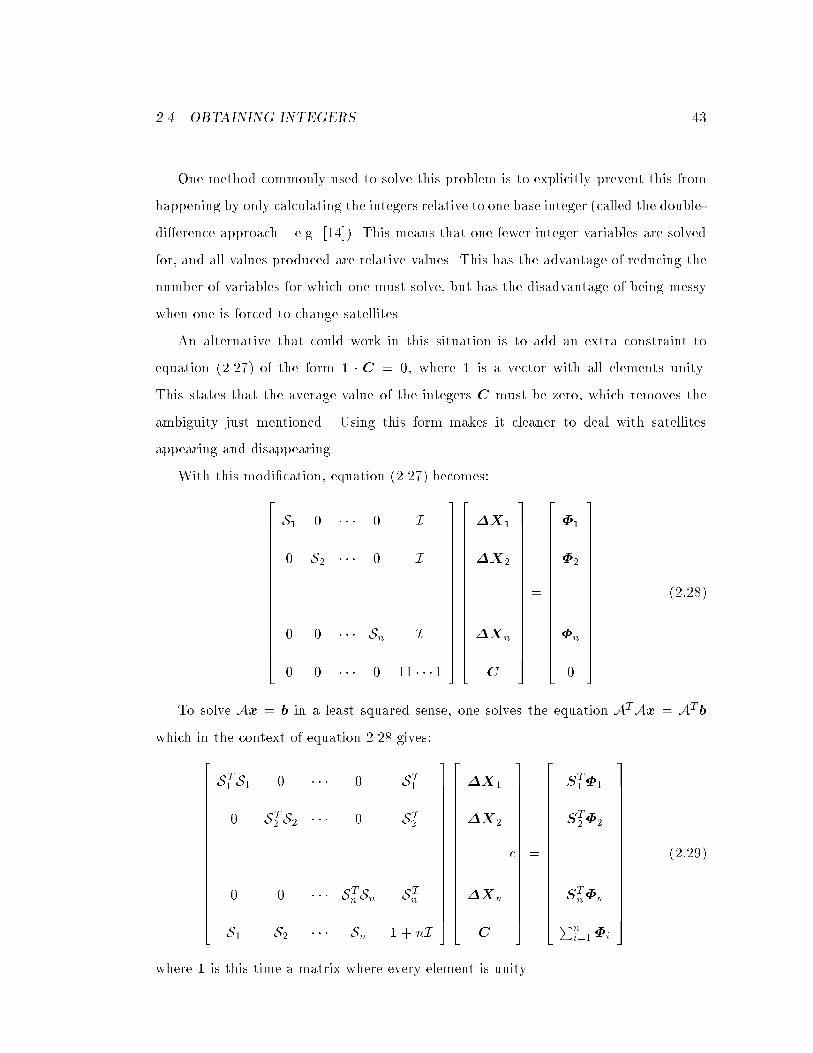
2.4. OBTAINING INTEGERS 43
One method commonly used to solve this problem is to explicitly prevent this from
happening by only calculating the integers relative to one base integer (called the double-
di�erence approach { e.g. [14]). This means that one fewer integer variables are solved
for, and all values produced are relative values. This has the advantage of reducing the
number of variables for which one must solve, but has the disadvantage of being messy
when one is forced to change satellites.
An alternative that could work in this situation is to add an extra constraint to
equation (2.27) of the form 1 � C = 0, where 1 is a vector with all elements unity.
This states that the average value of the integers C must be zero, which removes the
ambiguity just mentioned. Using this form makes it cleaner to deal with satellites
appearing and disappearing.
With this modi�cation, equation (2.27) becomes:
2666666666666666664
S1 0 � � � 0 I
0 S2 � � � 0 I...
0 0 � � � Sn I
0 0 � � � 0 11 � � �1
3777777777777777775
2666666666666666664
�X1
�X2
...
�Xn
C
3777777777777777775
=
2666666666666666664
�1
�2
...
�n
0
3777777777777777775
(2:28)
To solve Ax = b in a least squared sense, one solves the equation ATAx = ATb
which in the context of equation 2.28 gives:
2666666666666666664
ST1 S1 0 � � � 0 ST1
0 ST2 S2 � � � 0 ST2...
0 0 � � � STn Sn STn
S1 S2 � � � Sn 1+ nI
3777777777777777775
2666666666666666664
�X1
�X2
...
�Xn
C
c
3777777777777777775
=
2666666666666666664
ST1�1
ST2�2
...
STn�n
Pni=1�i
3777777777777777775
(2:29)
where 1 is this time a matrix where every element is unity.
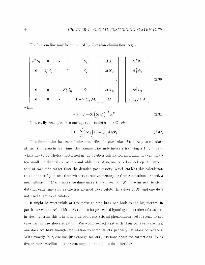
44 CHAPTER 2. GLOBAL POSITIONING SYSTEM (GPS)
The bottom line may be simpli�ed by Gaussian elimination to get
2666666666666666664
ST1 S1 0 � � � 0 ST1
0 ST2 S2 � � � 0 ST2...
0 0 � � � STn Sn STn
0 0 � � � 0 1+Pn
i=1Mi
3777777777777777775
2666666666666666664
�X1
�X2
...
�Xn
C
c
3777777777777777775
=
2666666666666666664
ST1�1
ST2�2
...
STn�n
Pni=1Mi�i
3777777777777777775
(2:30)
where
Mi = I � Si�STi Si
��1 STi (2:31)
This easily decouples into one equation to determine C , viz. 1 +
nXi=1
Mi
!C =
nXi=1
Mi�i (2:32)
This formulation has several nice properties. In particular, Mi is easy to calculate
at each time step in real time: this computation only involves inverting a 4 by 4 array
which has to be Cholsky factorised in the position calculation algorithm anyway plus a
few small matrix multiplications and additions. Also, one only has to keep the current
sum of each side rather than the detailed past history, which enables this calculation
to be done easily in real time without excessive memory or time constraints. Indeed, a
new estimate of C can easily be done many times a second. We have no need to store
data for each time step as one has no need to calculate the values of X i and one does
not need them to calculate Ci.
It might be worthwhile at this point to step back and look at the big picture, in
particular matrixMi. This derivation so far proceeded ignoring the number of satellites
in view, whereas this is in reality an obviously critical phenomenon, yet it seems to not
take part in the above equation. We would expect that with three or fewer satellites,
one does not have enough information to compute �x properly, let alone corrections.
With exactly four, one has just enough for �x, but none spare for corrections. With
�ve or more satellites in view one ought to be able to do something.
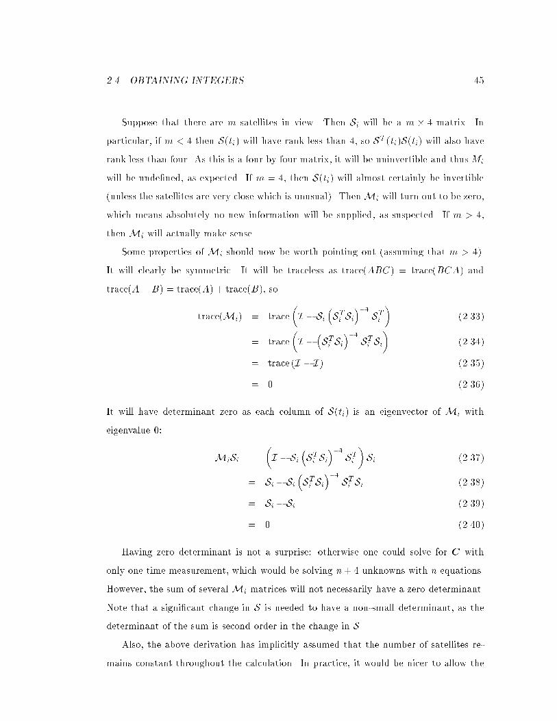
2.4. OBTAINING INTEGERS 45
Suppose that there are m satellites in view. Then Si will be a m � 4 matrix. In
particular, if m < 4 then S(ti) will have rank less than 4, so ST (ti)S(ti) will also have
rank less than four. As this is a four by four matrix, it will be uninvertible and thusMi
will be unde�ned, as expected. If m = 4, then S(ti) will almost certainly be invertible
(unless the satellites are very close which is unusual). ThenMi will turn out to be zero,
which means absolutely no new information will be supplied, as suspected. If m > 4,
thenMi will actually make sense.
Some properties of Mi should now be worth pointing out (assuming that m > 4).
It will clearly be symmetric. It will be traceless as trace(ABC) = trace(BCA) and
trace(A+ B) = trace(A) + trace(B), so
trace(Mi) = trace
�I � Si
�STi Si
��1 STi�
(2.33)
= trace
�I �
�STi Si
��1 STi Si�
(2.34)
= trace (I � I) (2.35)
= 0 (2.36)
It will have determinant zero as each column of S(ti) is an eigenvector of Mi with
eigenvalue 0:
MiSi =
�I � Si
�STi Si
��1 STi�Si (2.37)
= Si � Si�STi Si
��1 STi Si (2.38)
= Si � Si (2.39)
= 0 (2.40)
Having zero determinant is not a surprise: otherwise one could solve for C with
only one time measurement, which would be solving n+ 4 unknowns with n equations.
However, the sum of severalMi matrices will not necessarily have a zero determinant.
Note that a signi�cant change in S is needed to have a non-small determinant, as the
determinant of the sum is second order in the change in S.Also, the above derivation has implicitly assumed that the number of satellites re-
mains constant throughout the calculation. In practice, it would be nicer to allow the
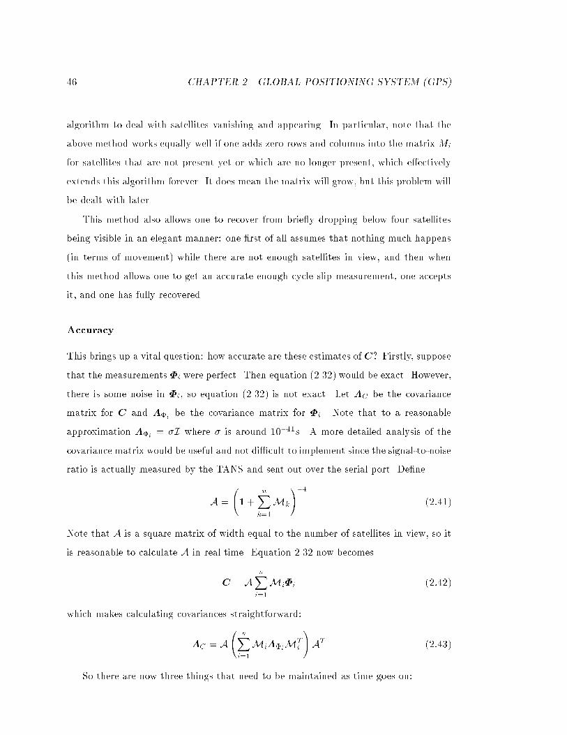
46 CHAPTER 2. GLOBAL POSITIONING SYSTEM (GPS)
algorithm to deal with satellites vanishing and appearing. In particular, note that the
above method works equally well if one adds zero rows and columns into the matrix Mi
for satellites that are not present yet or which are no longer present, which e�ectively
extends this algorithm forever. It does mean the matrix will grow, but this problem will
be dealt with later.
This method also allows one to recover from brie y dropping below four satellites
being visible in an elegant manner: one �rst of all assumes that nothing much happens
(in terms of movement) while there are not enough satellites in view, and then when
this method allows one to get an accurate enough cycle slip measurement, one accepts
it, and one has fully recovered.
Accuracy
This brings up a vital question: how accurate are these estimates of C? Firstly, suppose
that the measurements �i were perfect. Then equation (2.32) would be exact. However,
there is some noise in �i, so equation (2.32) is not exact. Let �C be the covariance
matrix for C and ��ibe the covariance matrix for �i. Note that to a reasonable
approximation ��i= �I where � is around 10�11s. A more detailed analysis of the
covariance matrix would be useful and not di�cult to implement since the signal-to-noise
ratio is actually measured by the TANS and sent out over the serial port. De�ne
A =
1+
nXk=1
Mk
!�1
(2:41)
Note that A is a square matrix of width equal to the number of satellites in view, so it
is reasonable to calculate A in real time. Equation 2.32 now becomes
C = AnX
i=1
Mi�i (2:42)
which makes calculating covariances straightforward:
�C = A
nXi=1
Mi��iMT
i
!AT (2:43)
So there are now three things that need to be maintained as time goes on:
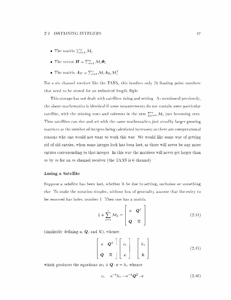
2.4. OBTAINING INTEGERS 47
� The matrixPn
i=1Mi
� The vector H =Pn
i=1Mi�i
� The matrix �H =Pn
i=1Mi��iMT
i .
For a six channel receiver like the TANS, this involves only 78 oating point numbers
that need to be stored for an unlimited length ight.
This storage has not dealt with satellites rising and setting. As mentioned previously,
the above mathematics is identical if some measurements do not contain some particular
satellite, with the missing rows and columns in the sumPn
i=1Mi just becoming zero.
Thus satellites can rise and set with the same mathematics; just steadily larger growing
matrices as the number of integers being calculated increases; so there are computational
reasons why one would not want to work this way. We would like some way of getting
rid of old entries, when some integer lock has been lost, as there will never be any more
entries corresponding to that integer. In this way the matrices will never get larger than
m by m for an m channel receiver (the TANS is 6 channel).
Losing a Satellite
Suppose a satellite has been lost, whether it be due to setting, occlusion or something
else. To make the notation simpler, without loss of generality assume that the entry to
be removed has index number 1. Then one has a matrix
1+nX
k=1
Mk =
26664a QT
Q R
37775 (2:44)
(implicitly de�ning a, Q, and R), whence26664a QT
Q R
3777526664c1
c
37775 =
26664h1
h
37775 (2:45)
which produces the equations ac1 +Q � c = h1 whence
c1 = a�1h1 � a�1QT � c (2:46)
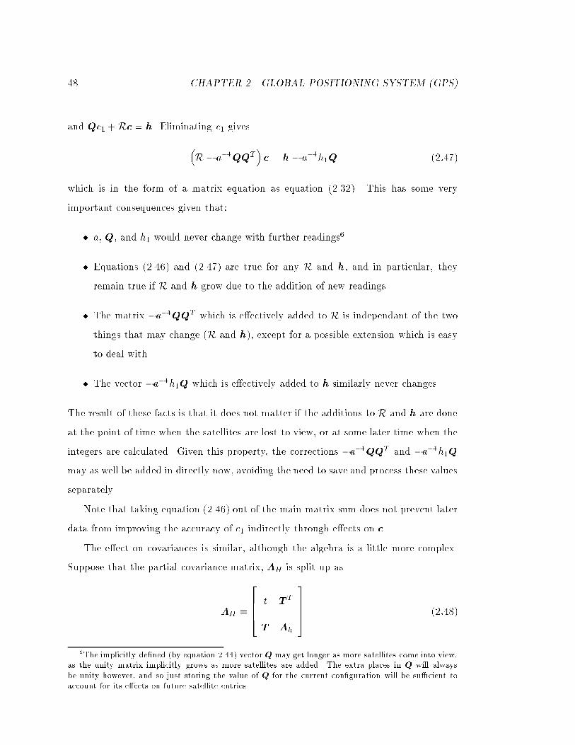
48 CHAPTER 2. GLOBAL POSITIONING SYSTEM (GPS)
and Qc1 +Rc = h. Eliminating c1 gives�R� a�1QQT
�c = h � a�1h1Q (2:47)
which is in the form of a matrix equation as equation (2.32). This has some very
important consequences given that:
� a, Q, and h1 would never change with further readings6.
� Equations (2.46) and (2.47) are true for any R and h, and in particular, they
remain true if R and h grow due to the addition of new readings
� The matrix �a�1QQT which is e�ectively added to R is independant of the two
things that may change (R and h), except for a possible extension which is easy
to deal with.
� The vector �a�1h1Q which is e�ectively added to h similarly never changes.
The result of these facts is that it does not matter if the additions to R and h are done
at the point of time when the satellites are lost to view, or at some later time when the
integers are calculated. Given this property, the corrections �a�1QQT and �a�1h1Qmay as well be added in directly now, avoiding the need to save and process these values
separately.
Note that taking equation (2.46) out of the main matrix sum does not prevent later
data from improving the accuracy of c1 indirectly through e�ects on c.
The e�ect on covariances is similar, although the algebra is a little more complex.
Suppose that the partial covariance matrix, �H is split up as
�H =
26664t T T
T �h
37775 (2:48)
6The implicitly de�ned (by equation 2.44) vector Q may get longer as more satellites come into view,as the unity matrix implicitly grows as more satellites are added. The extra places in Q will alwaysbe unity however, and so just storing the value of Q for the current con�guration will be su�cient toaccount for its e�ects on future satellite entries.
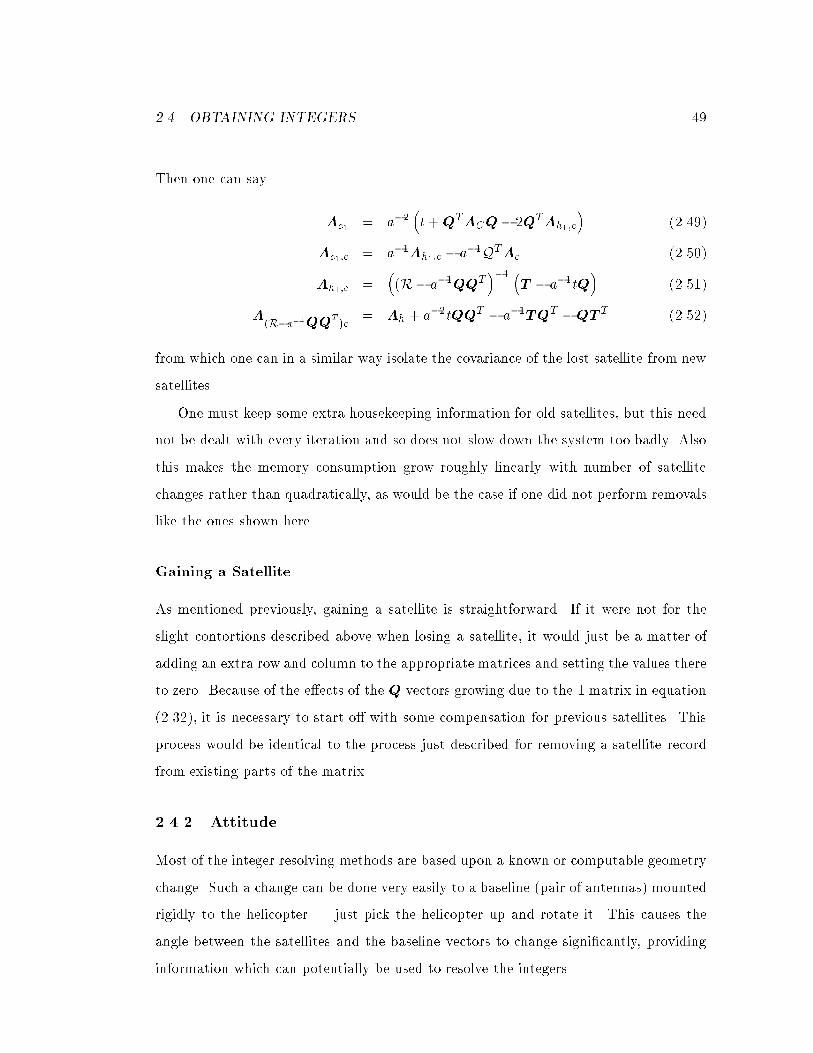
2.4. OBTAINING INTEGERS 49
Then one can say
�c1 = a�2�t +QT�CQ� 2QT�h1;c
�(2.49)
�c1;c = a�1�h1;c � a�1QT�c (2.50)
�h1;c =�(R� a�1QQT
��1 �T � a�1tQ
�(2.51)
�(R�a�1QQ
T)c
= �h + a�2tQQT � a�1TQT �QT T (2.52)
from which one can in a similar way isolate the covariance of the lost satellite from new
satellites.
One must keep some extra housekeeping information for old satellites, but this need
not be dealt with every iteration and so does not slow down the system too badly. Also
this makes the memory consumption grow roughly linearly with number of satellite
changes rather than quadratically, as would be the case if one did not perform removals
like the ones shown here.
Gaining a Satellite
As mentioned previously, gaining a satellite is straightforward. If it were not for the
slight contortions described above when losing a satellite, it would just be a matter of
adding an extra row and column to the appropriate matrices and setting the values there
to zero. Because of the e�ects of the Q vectors growing due to the 1 matrix in equation
(2.32), it is necessary to start o� with some compensation for previous satellites. This
process would be identical to the process just described for removing a satellite record
from existing parts of the matrix.
2.4.2 Attitude
Most of the integer resolving methods are based upon a known or computable geometry
change. Such a change can be done very easily to a baseline (pair of antennas) mounted
rigidly to the helicopter | just pick the helicopter up and rotate it. This causes the
angle between the satellites and the baseline vectors to change signi�cantly, providing
information which can potentially be used to resolve the integers.
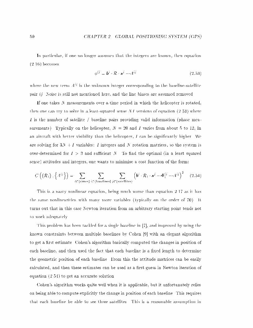
50 CHAPTER 2. GLOBAL POSITIONING SYSTEM (GPS)
In particular, if one no longer assumes that the integers are known, then equation
(2.16) becomes
�ij = bi � R � sj �Aij (2:53)
where the new term Aij is the unknown integer corresponding to the baseline-satellite
pair ij. Noise is still not mentioned here, and the line biases are assumed removed.
If one takes N measurements over a time period in which the helicopter is rotated,
then one can try to solve in a least-squared sense NI versions of equation (2.53) where
I is the number of satellite / baseline pairs providing valid information (phase mea-
surements). Typically on the helicopter, N = 20 and I varies from about 5 to 12, In
an aircraft with better visibility than the helicopter, I can be signi�cantly higher. We
are solving for 3N + I variables: I integers and N rotation matrices, so the system is
over-determined for I > 3 and su�cient N . To �nd the optimal (in a least squared
sense) attitudes and integers, one wants to minimise a cost function of the form:
C�fRtg ;
nAijo�
=X
t2ftimesg
Xi2fbaselinesg
Xj2fsatellitesg
�bi � Rt � sj � �ij
t �Aij�2
(2:54)
This is a nasty nonlinear equation, being much worse than equation 2.17 as it has
the same nonlinearities with many more variables (typically on the order of 70). It
turns out that in this case Newton iteration from an arbitrary starting point tends not
to work adequately.
This problem has been tackled for a single baseline in [7], and improved by using the
known constraints between multiple baselines by Cohen [9] with an elegant algorithm
to get a �rst estimate. Cohen's algorithm basically computed the changes in position of
each baseline, and then used the fact that each baseline is a �xed length to determine
the geometric position of each baseline. From this the attitude matrices can be easily
calculated, and then these estimates can be used as a �rst guess in Newton iteration of
equation (2.54) to get an accurate solution.
Cohen's algorithm works quite well when it is applicable, but it unfortunately relies
on being able to compute explicitly the change in position of each baseline. This requires
that each baseline be able to see three satellites. This is a reasonable assumption in
2.4. OBTAINING INTEGERS 51
many applications, but it is not reasonable on the helicopter due to the poor visibility
of the side antennas due to occlusion and lack of space for ground planes.
For these reasons, it was necessary to come up with a new algorithm, and it was
for this reason that the pseudo-global solution described in detail in section 2.3.5 was
developed. For the algorithm in section 2.3.5 generalises easily fromminimising equation
2.17 to equation 2.54. One iteration of the pseudo-global algorithm now consists of doing
a global minimisation on the three attitude parameters for each time period sequentially,
followed by the integers.
Minimising with respect to an attitude parameter for a given time period follows
almost exactly the same steps described in section 2.3.5. Equation (2.19) has now
changed to
C (t) =
Xi2fbaselinesgj2fsatellitesg
0BBBBBBBB@bi �
2666666664
cost sin t 0
� sint cost 0
0 0 1
3777777775Rt � sj � �ij
t
1CCCCCCCCA
2
+costs independent of t
(2.55)
= c1 cos2+ c2 sin
2+ c3 cos sin + c4 cos + c5 sin + c6 (2.56)
Equation (2.56) is now in the same form as equation (2.21), and the optimal value
of can then be obtained in exactly the same way as in section 2.3.5.
After processing the 3N angle variables, it is necessary to minimise the integers.
This is straightforward: the best estimate of an integer Aij is given by
Aij =1
N
Xt2ftimesg
bi � R � sj � �ij (2:57)
One iteration of the pseudo-global algorithm then consists of minimising with respect
to 3N attitude variables and then the I integers. As previously, the pseudo-global
algorithm works better than Newton iteration with a poor initial guess (such as all
attitudes starting the same, and the integers starting o� as the average of the phases),
and Newton iteration converges more rapidly when one is near the solution.
52 CHAPTER 2. GLOBAL POSITIONING SYSTEM (GPS)
As a slight variation on this algorithm, the global minimisation can be performed
with respect to only azimuth on the �rst iteration if it is known that most of the angular
movement is going to be in azimuth. This can increase the rate of convergence. Another
slight variation is to modify the local iteration step to do a pseudo-global step if the
matrices used in its calculation ever become too badly ill conditioned (which happens
occasionally). This will increase reliability.
An algorithm to actually minimise equation 2.54 consists of several iterations of the
pseudo-global or local algorithms. Simulation showed that about 20 iterations of the
pseudo-global algorithm were needed to get a reasonable �rst estimate for the local
algorithm, which is then applied until the cost function stops decreasing.7 A slightly
better algorithm still consists of alternating pairs of pseudo-global and local iteration
steps. The reason for dividing into pairs is that a local step can often cause the solution
to jump along a valley, vastly increasing the cost function, and a second local iteration
is usually better at repairing this damage than a pseudo-global iteration.
Once a minimum cost has been reached, one must decide whether the solution is rea-
sonable...for this algorithm is by no means guaranteed to converge { sometimes because
the problem is ill posed (the geometry does not contain enough information or the loss
of precision due to geometric dilution of precision is too high), and sometimes because
this algorithm is by no means perfect. Fortunately there are three methods of checking
the result for reasonableness. Firstly, the value of the cost function must be su�ciently
low as to be accounted for by noise and not some more serious problem. Secondly, the
\integers" Aij which were estimated as continuous values should be fairly near integral
values. Thirdly, as these integers are used in the future in operational attitude solutions,
if the resulting residuals are too high then there is probably a problem with them.
The way the helicopter system currently works is that the attitude integers are
initialised by picking up the helicopter and rotating it. After it has acquired the integers8
the helicopter can be rotated a little more for this additional level of safety. The integers
could also be acquired from a rotation in- ight whilst under manual control. This is
7An increase on the �rst local iteration is common and is not counted.8This is indicated by beeping and on a seven segment LED display
2.4. OBTAINING INTEGERS 53
not done due to desire to check that the integer resolution worked and to the di�culty
in performing such a maneuver manually.
To increase reliability ever further, here are two possible suggestions. Firstly, one can
store the phase measurements for the seconds preceding and during integer resolution9,
and use them for veri�cation. Secondly, it is straightforward to compute the partial
derivative of changes in Aij to input phases, and this can be used to get an estimate
of the expected noise in the integers. This can be used to improve the accuracy of the
decision as to whether they are too far o� integer values to be reasonable. Neither were
implemented as they did not seem necessary and would increase the time for integer
resolution: the �rst involves storage and replay; the second involves inversion of a fairly
large matrix.
Some results of simulation are shown in �gures 2.8, 2.9 and 2.10. The simulated
data is for a roughly 180 degree turn, with twenty time steps and I averaging 6:5, and
never dropping below 5. Note that Cohen's algorithm requires I to be at least 9, and
only some speci�c patterns of 9 really work.
The base case for comparison is Newton's method (�gure 2.8). In practice, this
did work a reasonable proportion of the time (45 percent). Figure 2.8 shows how the
cost functions behaved during this algorithm (a hundred examples are shown simulta-
neously). Using twenty iterations of the pseudo-global algorithm instead of Newton's
algorithm on exactly the same test cases worked 73 percent (�gure 2.9), and the alter-
nation worked 86 percent of the time (�gure 2.10). Reducing the number of satellites
visible to 5 or 6 reduces these �gures to 29, 58 and 70 percent respectively.
Of more importance, this algorithm was tested in practice on real data on the he-
licopter where it performed admirably. One rotation was usually su�cient to initialise
the attitude. The largest (practical) problem was putting the helicopter down without
obscuring the antennas.
9The integer resolution process takes under a second on the 33MHz 486 in the helicopter.
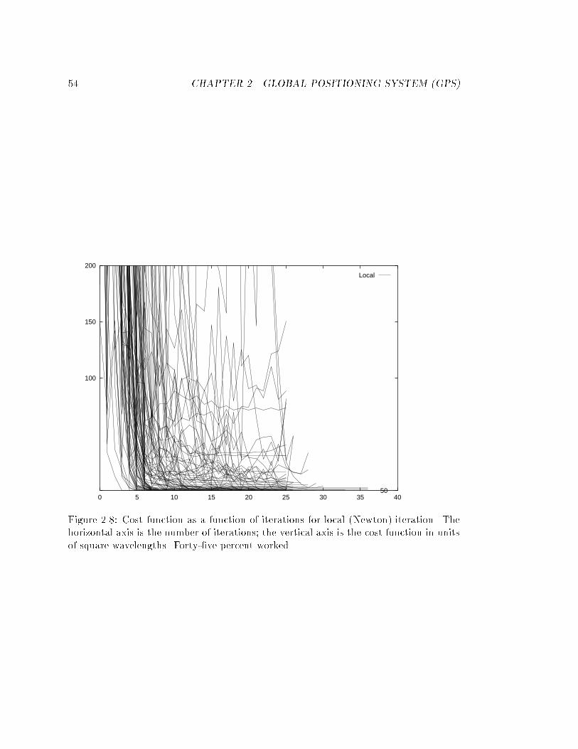
54 CHAPTER 2. GLOBAL POSITIONING SYSTEM (GPS)
50
100
150
200
0 5 10 15 20 25 30 35 40
Local
Figure 2.8: Cost function as a function of iterations for local (Newton) iteration. Thehorizontal axis is the number of iterations; the vertical axis is the cost function in unitsof square wavelengths. Forty-�ve percent worked.
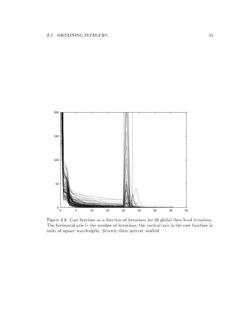
2.4. OBTAINING INTEGERS 55
0
50
100
150
200
0 5 10 15 20 25 30 35 40
Figure 2.9: Cost function as a function of iterations for 20 global then local iterations.The horizontal axis is the number of iterations; the vertical axis is the cost function inunits of square wavelengths. Seventy-three percent worked.
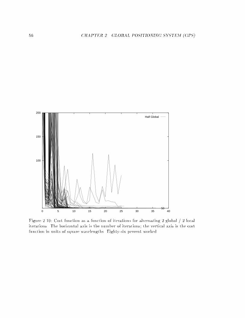
56 CHAPTER 2. GLOBAL POSITIONING SYSTEM (GPS)
50
100
150
200
0 5 10 15 20 25 30 35 40
Half Global
Figure 2.10: Cost function as a function of iterations for alternating 2 global / 2 localiterations. The horizontal axis is the number of iterations; the vertical axis is the costfunction in units of square wavelengths. Eighty-six percent worked.
Chapter 3
Hardware
This chapter describes the hardware used in this project, consisting of the helicopter
itself, the electronics on the helicopter, the ground station electronics, and some of the
support equipment. Details of connections, power supplies and mounting are supplied
in the appendices.
3.1 Helicopter
The main design objectives, which were satis�ed to varying degrees, when choosing the
helicopter were
� Payload capability.
� Inherent dynamics. (A helicopter in hover is inherently unstable.)
� Low vibration.
� Mechanical Strength.
� Control Authority.
� Durability.
� Ease of construction.
� Ease of replacement.
57
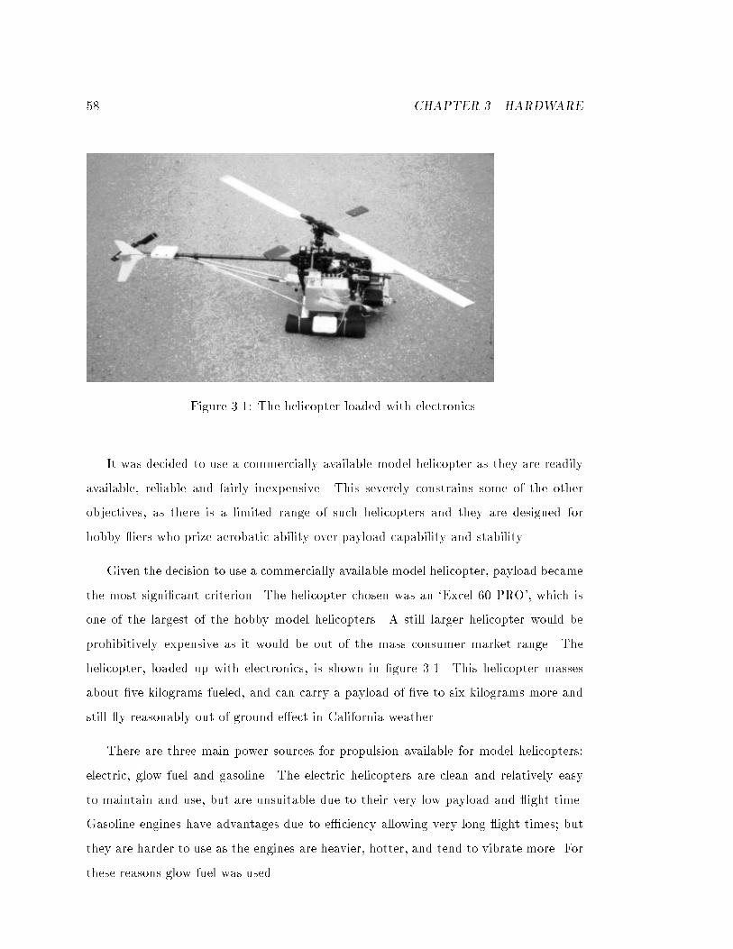
58 CHAPTER 3. HARDWARE
Figure 3.1: The helicopter loaded with electronics.
It was decided to use a commercially available model helicopter as they are readily
available, reliable and fairly inexpensive. This severely constrains some of the other
objectives, as there is a limited range of such helicopters and they are designed for
hobby iers who prize aerobatic ability over payload capability and stability.
Given the decision to use a commercially available model helicopter, payload became
the most signi�cant criterion. The helicopter chosen was an `Excel 60 PRO', which is
one of the largest of the hobby model helicopters. A still larger helicopter would be
prohibitively expensive as it would be out of the mass consumer market range. The
helicopter, loaded up with electronics, is shown in �gure 3.1. This helicopter masses
about �ve kilograms fueled, and can carry a payload of �ve to six kilograms more and
still y reasonably out of ground e�ect in California weather.
There are three main power sources for propulsion available for model helicopters:
electric, glow fuel and gasoline. The electric helicopters are clean and relatively easy
to maintain and use, but are unsuitable due to their very low payload and ight time.
Gasoline engines have advantages due to e�ciency allowing very long ight times; but
they are harder to use as the engines are heavier, hotter, and tend to vibrate more. For
these reasons glow fuel was used.
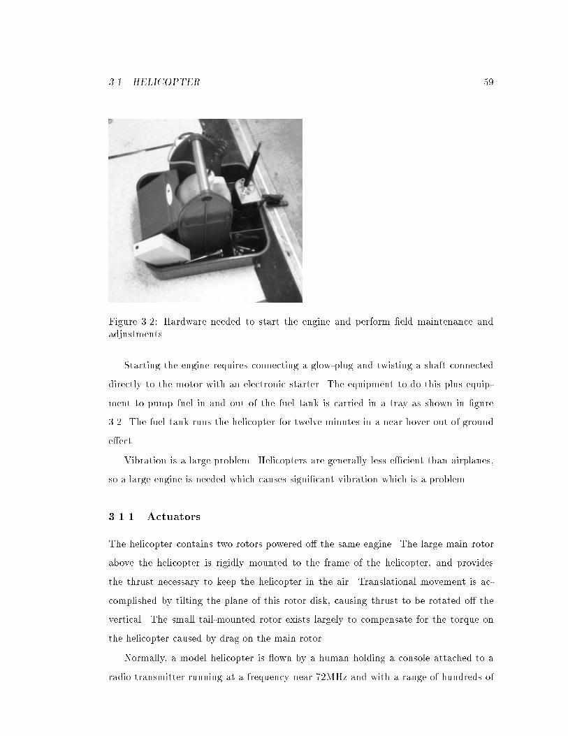
3.1. HELICOPTER 59
Figure 3.2: Hardware needed to start the engine and perform �eld maintenance andadjustments
Starting the engine requires connecting a glow-plug and twisting a shaft connected
directly to the motor with an electronic starter. The equipment to do this plus equip-
ment to pump fuel in and out of the fuel tank is carried in a tray as shown in �gure
3.2. The fuel tank runs the helicopter for twelve minutes in a near hover out of ground
e�ect.
Vibration is a large problem. Helicopters are generally less e�cient than airplanes,
so a large engine is needed which causes signi�cant vibration which is a problem.
3.1.1 Actuators
The helicopter contains two rotors powered o� the same engine. The large main rotor
above the helicopter is rigidly mounted to the frame of the helicopter, and provides
the thrust necessary to keep the helicopter in the air. Translational movement is ac-
complished by tilting the plane of this rotor disk, causing thrust to be rotated o� the
vertical. The small tail-mounted rotor exists largely to compensate for the torque on
the helicopter caused by drag on the main rotor.
Normally, a model helicopter is own by a human holding a console attached to a
radio transmitter running at a frequency near 72MHz and with a range of hundreds of
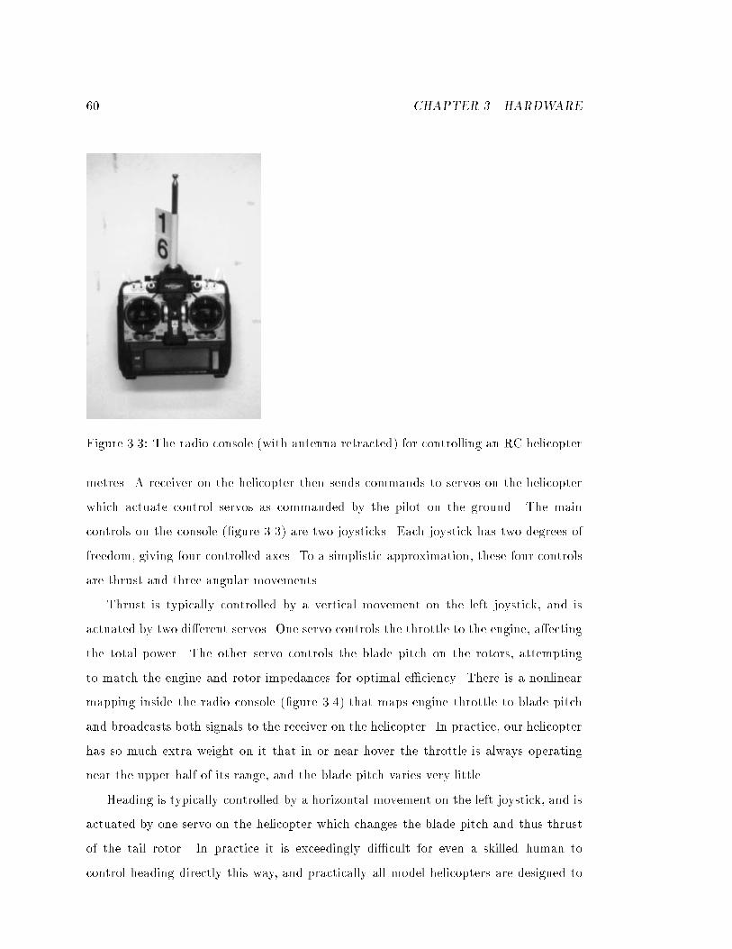
60 CHAPTER 3. HARDWARE
Figure 3.3: The radio console (with antenna retracted) for controlling an RC helicopter
metres. A receiver on the helicopter then sends commands to servos on the helicopter
which actuate control servos as commanded by the pilot on the ground. The main
controls on the console (�gure 3.3) are two joysticks. Each joystick has two degrees of
freedom, giving four controlled axes. To a simplistic approximation, these four controls
are thrust and three angular movements.
Thrust is typically controlled by a vertical movement on the left joystick, and is
actuated by two di�erent servos. One servo controls the throttle to the engine, a�ecting
the total power. The other servo controls the blade pitch on the rotors, attempting
to match the engine and rotor impedances for optimal e�ciency. There is a nonlinear
mapping inside the radio console (�gure 3.4) that maps engine throttle to blade pitch
and broadcasts both signals to the receiver on the helicopter. In practice, our helicopter
has so much extra weight on it that in or near hover the throttle is always operating
near the upper half of its range, and the blade pitch varies very little.
Heading is typically controlled by a horizontal movement on the left joystick, and is
actuated by one servo on the helicopter which changes the blade pitch and thus thrust
of the tail rotor. In practice it is exceedingly di�cult for even a skilled human to
control heading directly this way, and practically all model helicopters are designed to
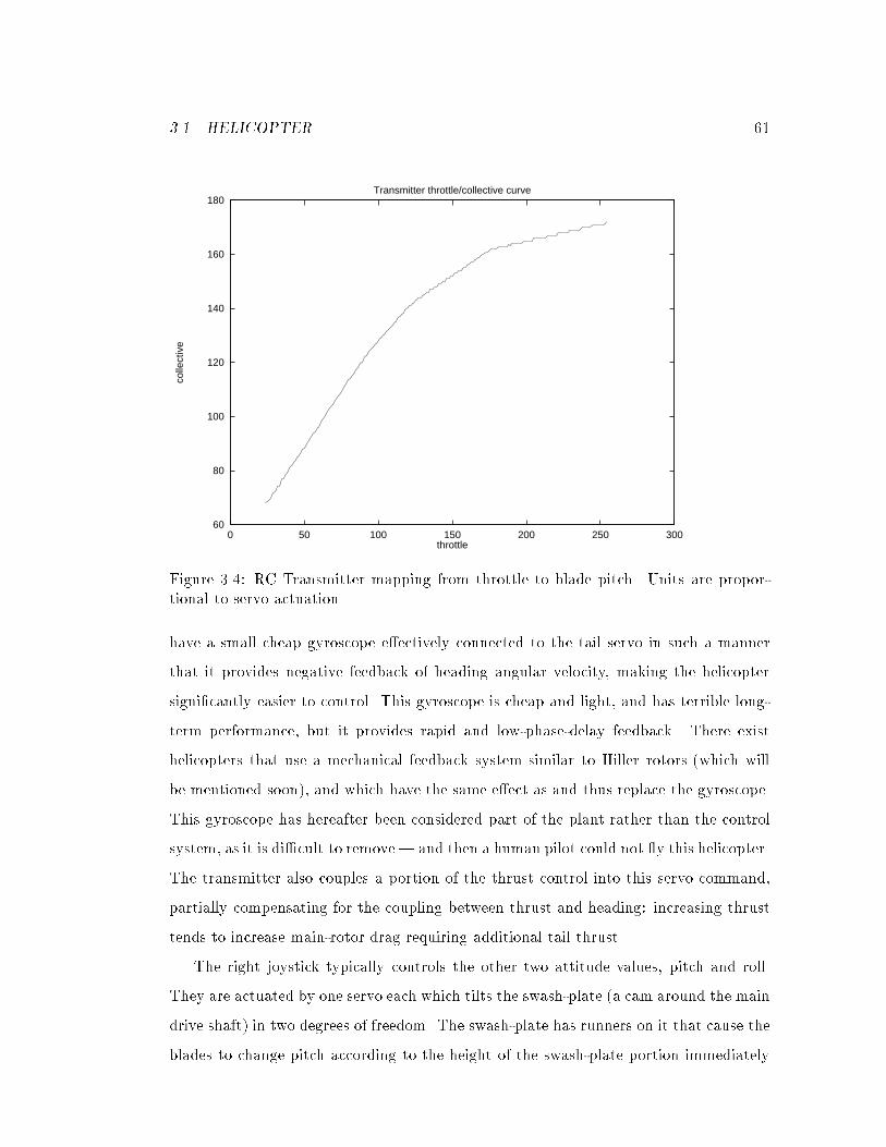
3.1. HELICOPTER 61
60
80
100
120
140
160
180
0 50 100 150 200 250 300
colle
ctiv
e
throttle
Transmitter throttle/collective curve
Figure 3.4: RC Transmitter mapping from throttle to blade pitch. Units are propor-tional to servo actuation
have a small cheap gyroscope e�ectively connected to the tail servo in such a manner
that it provides negative feedback of heading angular velocity, making the helicopter
signi�cantly easier to control. This gyroscope is cheap and light, and has terrible long-
term performance, but it provides rapid and low-phase-delay feedback. There exist
helicopters that use a mechanical feedback system similar to Hiller rotors (which will
be mentioned soon), and which have the same e�ect as and thus replace the gyroscope.
This gyroscope has hereafter been considered part of the plant rather than the control
system, as it is di�cult to remove| and then a human pilot could not y this helicopter.
The transmitter also couples a portion of the thrust control into this servo command,
partially compensating for the coupling between thrust and heading: increasing thrust
tends to increase main-rotor drag requiring additional tail thrust.
The right joystick typically controls the other two attitude values, pitch and roll.
They are actuated by one servo each which tilts the swash-plate (a cam around the main
drive shaft) in two degrees of freedom. The swash-plate has runners on it that cause the
blades to change pitch according to the height of the swash-plate portion immediately
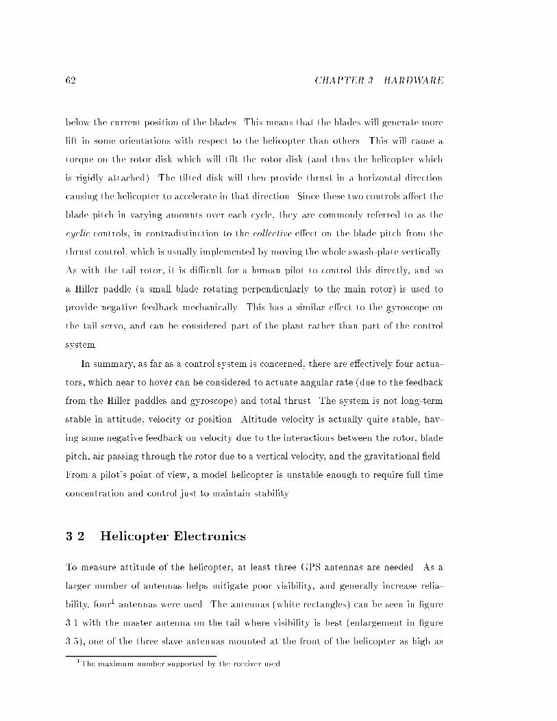
62 CHAPTER 3. HARDWARE
below the current position of the blades. This means that the blades will generate more
lift in some orientations with respect to the helicopter than others. This will cause a
torque on the rotor disk which will tilt the rotor disk (and thus the helicopter which
is rigidly attached). The tilted disk will then provide thrust in a horizontal direction
causing the helicopter to accelerate in that direction. Since these two controls a�ect the
blade pitch in varying amounts over each cycle, they are commonly referred to as the
cyclic controls, in contradistinction to the collective e�ect on the blade pitch from the
thrust control, which is usually implemented by moving the whole swash-plate vertically.
As with the tail rotor, it is di�cult for a human pilot to control this directly, and so
a Hiller paddle (a small blade rotating perpendicularly to the main rotor) is used to
provide negative feedback mechanically. This has a similar e�ect to the gyroscope on
the tail servo, and can be considered part of the plant rather than part of the control
system.
In summary, as far as a control system is concerned, there are e�ectively four actua-
tors, which near to hover can be considered to actuate angular rate (due to the feedback
from the Hiller paddles and gyroscope) and total thrust. The system is not long-term
stable in attitude, velocity or position. Altitude velocity is actually quite stable, hav-
ing some negative feedback on velocity due to the interactions between the rotor, blade
pitch, air passing through the rotor due to a vertical velocity, and the gravitational �eld.
From a pilot's point of view, a model helicopter is unstable enough to require full time
concentration and control just to maintain stability.
3.2 Helicopter Electronics
To measure attitude of the helicopter, at least three GPS antennas are needed. As a
larger number of antennas helps mitigate poor visibility, and generally increase relia-
bility, four1 antennas were used. The antennas (white rectangles) can be seen in �gure
3.1 with the master antenna on the tail where visibility is best (enlargement in �gure
3.5), one of the three slave antennas mounted at the front of the helicopter as high as
1The maximum number supported by the receiver used.
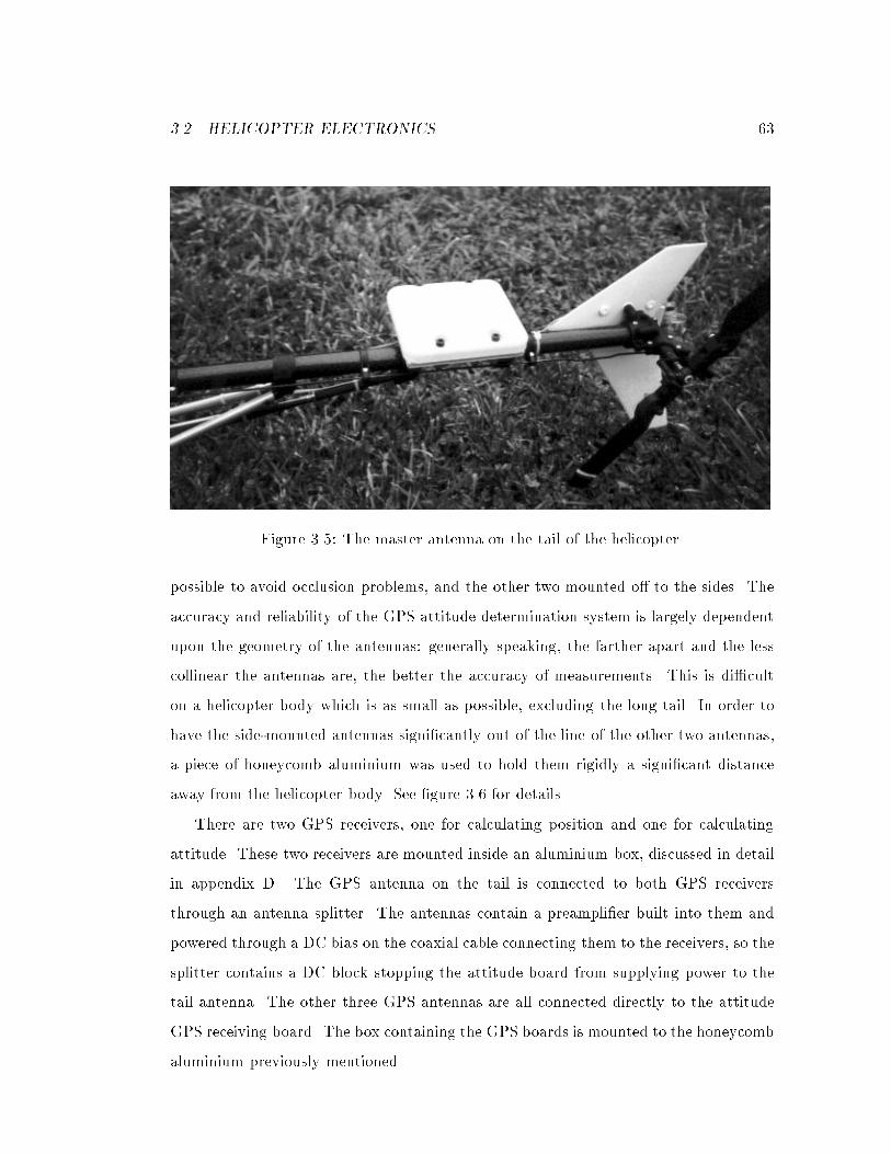
3.2. HELICOPTER ELECTRONICS 63
Figure 3.5: The master antenna on the tail of the helicopter.
possible to avoid occlusion problems, and the other two mounted o� to the sides. The
accuracy and reliability of the GPS attitude determination system is largely dependent
upon the geometry of the antennas: generally speaking, the farther apart and the less
collinear the antennas are, the better the accuracy of measurements. This is di�cult
on a helicopter body which is as small as possible, excluding the long tail. In order to
have the side-mounted antennas signi�cantly out of the line of the other two antennas,
a piece of honeycomb aluminium was used to hold them rigidly a signi�cant distance
away from the helicopter body. See �gure 3.6 for details.
There are two GPS receivers, one for calculating position and one for calculating
attitude. These two receivers are mounted inside an aluminium box, discussed in detail
in appendix D. The GPS antenna on the tail is connected to both GPS receivers
through an antenna splitter. The antennas contain a preampli�er built into them and
powered through a DC bias on the coaxial cable connecting them to the receivers, so the
splitter contains a DC block stopping the attitude board from supplying power to the
tail antenna. The other three GPS antennas are all connected directly to the attitude
GPS receiving board. The box containing the GPS boards is mounted to the honeycomb
aluminium previously mentioned.
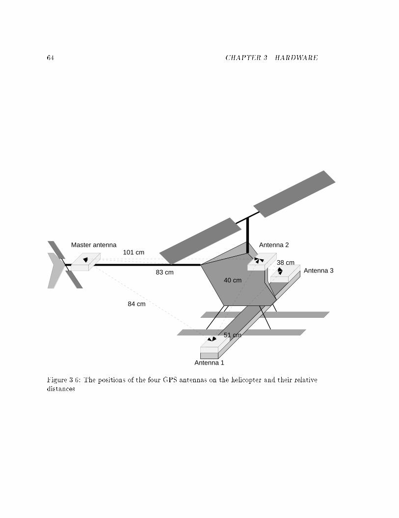
64 CHAPTER 3. HARDWARE
Master antenna
Antenna 1
Antenna 2
Antenna 3
84 cm
101 cm
83 cm40 cm
38 cm
51 cm
Figure 3.6: The positions of the four GPS antennas on the helicopter and their relativedistances.
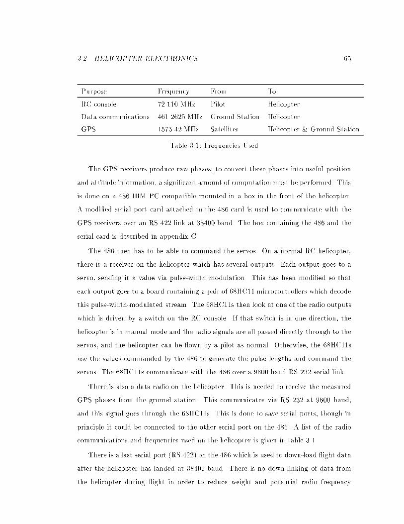
3.2. HELICOPTER ELECTRONICS 65
Purpose Frequency From To
RC console 72.110 MHz Pilot Helicopter
Data communications 461.2625 MHz Ground Station Helicopter
GPS 1575.42 MHz Satellites Helicopter & Ground Station
Table 3.1: Frequencies Used
The GPS receivers produce raw phases; to convert these phases into useful position
and attitude information, a signi�cant amount of computation must be performed. This
is done on a 486 IBM PC compatible mounted in a box in the front of the helicopter.
A modi�ed serial port card attached to the 486 card is used to communicate with the
GPS receivers over an RS 422 link at 38400 baud. The box containing the 486 and the
serial card is described in appendix C
The 486 then has to be able to command the servos. On a normal RC helicopter,
there is a receiver on the helicopter which has several outputs. Each output goes to a
servo, sending it a value via pulse-width modulation. This has been modi�ed so that
each output goes to a board containing a pair of 68HC11 microcontrollers which decode
this pulse-width-modulated stream. The 68HC11s then look at one of the radio outputs
which is driven by a switch on the RC console. If that switch is in one direction, the
helicopter is in manual mode and the radio signals are all passed directly through to the
servos, and the helicopter can be own by a pilot as normal. Otherwise, the 68HC11s
use the values commanded by the 486 to generate the pulse lengths and command the
servos. The 68HC11s communicate with the 486 over a 9600 baud RS 232 serial link.
There is also a data radio on the helicopter. This is needed to receive the measured
GPS phases from the ground station. This communicates via RS 232 at 9600 baud,
and this signal goes through the 68HC11s. This is done to save serial ports, though in
principle it could be connected to the other serial port on the 486. A list of the radio
communications and frequencies used on the helicopter is given in table 3.1
There is a last serial port (RS 422) on the 486 which is used to down-load ight data
after the helicopter has landed at 38400 baud. There is no down-linking of data from
the helicopter during ight in order to reduce weight and potential radio frequency
66 CHAPTER 3. HARDWARE
interference problems. This means that all computation is done on the helicopter.
Should the ground station vanish, the helicopter would then be unable to compute GPS
position, but would still be capable of attitude stabilisation.
To provide feedback to the helicopter operators, the parallel port on the 486 card
drives a seven segment LED display providing detailed status, and a pair of high e�-
ciency LEDs on the tail which ash every time a position �x is generated.
A summary of the electronic interconnections on the helicopter, excluding power
supplies is given in �gure 3.7.
Electrical power for the above circuitry comes from three batteries. The normal
method of powering the radio receiver and servos on an RC helicopter is via a small
4.8V to 5V battery pack containing four NiCd batteries. Two of these are used on this
helicopter; one powering the RC radio receiver and HC11s, and the other powering the
servos. This is all the circuitry needed for manual control to function, so if something
goes wrong with the rest of the circuitry, the helicopter should still be controllable.
The third battery is signi�cantly larger than the other two, being 7.2V with a ca-
pacity of 2.3Ah. This supplies the data radio, and, via 5V low-dropout regulators, the
486, serial card and GPS receivers.
A summary of the power system on the helicopter is shown in �gure 3.8.
As a last safety resort in case the 68HC11 board fails (which it never has yet), there
is a servo connected directly to the radio receiver which has the sole purpose of shutting
o� fuel to the engine.
3.3 Ground Station Electronics
The ground station electronics is much simpler than the helicopter electronics. There
is a GPS receiver connected to one GPS antenna and to a portable computer. The
portable computer initialises the GPS receiver, and then relays packets from the GPS
receiver to a radio data transmitter to be then received on board the helicopter. The
portable computer has its own battery pack. The GPS receiver and radio transmitter
are powered by a 12V battery and appropriate regulators. All this equipment �ts into
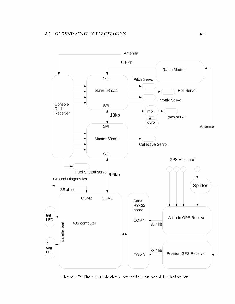
3.3. GROUND STATION ELECTRONICS 67
Splitter
Attitude GPS Receiver
Position GPS Receiver
COM2 COM1
COM4
COM3
Radio Modem
Antenna
GPS Antennae
Ground Diagnostics
Antenna
Slave 68hc11
SCI
SPI
SPI
SCI
Master 68hc11
ConsoleRadioReceiver
Fuel Shutoff servo
Collective Servo
gyro
mixyaw servo
Roll Servo
Pitch Servo
Throttle Servo
486 computer
SerialRS422board
para
llel p
ort
7segLED
tailLED
9.6kb
38.4 kb
38.4 kb
38.4 kb
13kb
9.6kb
Figure 3.7: The electronic signal connections on board the helicopter
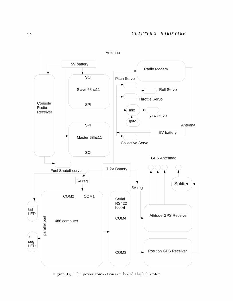
68 CHAPTER 3. HARDWARE
Splitter
Attitude GPS Receiver
Position GPS Receiver
COM2 COM1
COM4
COM3
Radio Modem
Antenna
GPS Antennae
Antenna
Slave 68hc11
SCI
SPI
SPI
SCI
Master 68hc11
ConsoleRadioReceiver
Fuel Shutoff servo
Collective Servo
gyro
mixyaw servo
Roll Servo
Pitch Servo
Throttle Servo
486 computer
SerialRS422board
7.2V Battery
5V battery
5V battery
5V reg
5V reg
para
llel p
ort
7segLED
tailLED
Figure 3.8: The power connections on board the helicopter
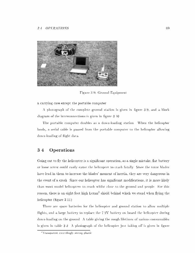
3.4. OPERATIONS 69
Figure 3.9: Ground Equipment
a carrying case except the portable computer.
A photograph of the complete ground station is given in �gure 3.9, and a block
diagram of the interconnections is given in �gure 3.10.
The portable computer doubles as a down-loading station. When the helicopter
lands, a serial cable is passed from the portable computer to the helicopter allowing
down-loading of ight data.
3.4 Operations
Going out to y the helicopter is a signi�cant operation, as a single mistake, at battery
or loose screw could easily cause the helicopter to crash fatally. Since the rotor blades
have lead in them to increase the blades' moment of inertia, they are very dangerous in
the event of a crash. Since our helicopter has signi�cant modi�cations, it is more likely
than most model helicopters to crash whilst close to the ground and people. For this
reason, there is an eight foot high Lexan2 shield behind which we stand when ying the
helicopter (�gure 3.11).
There are spare batteries for the helicopter and ground station to allow multiple
ights, and a large battery to replace the 7.2V battery on board the helicopter during
down-loading on the ground. A table giving the rough lifetimes of various consumables
is given in table 3.2. A photograph of the helicopter just taking o� is given in �gure
2Transparent exceedingly strong plastic
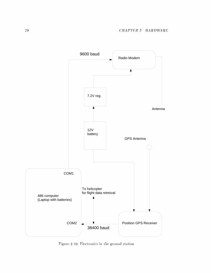
70 CHAPTER 3. HARDWARE
Position GPS ReceiverCOM2
COM1
Radio Modem
Antenna
GPS Antenna
486 computer(Laptop with batteries)
To helicopterfor flight data retreival
12Vbattery
7.2V reg.
9600 baud
38400 baud
Figure 3.10: Electronics in the ground station
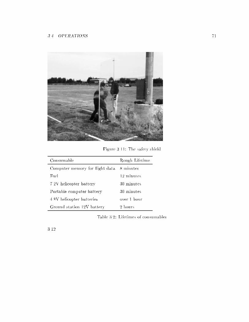
3.4. OPERATIONS 71
Figure 3.11: The safety shield
Consumable Rough Lifetime
Computer memory for ight data 8 minutes
Fuel 12 minutes
7.2V helicopter battery 30 minutes
Portable computer battery 30 minutes
4.8V helicopter batteries over 1 hour
Ground station 12V battery 2 hours
Table 3.2: Lifetimes of consumables
3.12.

72 CHAPTER 3. HARDWARE
Figure 3.12: The helicopter taking o�, as seen through the shield.
Chapter 4
Software
As seen in the hardware chapter, there are several computers in this system:
� The 486 on the helicopter
� The two 68HC11s
� The ground station
These computers have to do di�erent things at di�erent times, and there is also post
processing to be done. This chapter describes the design, functionality and philosophy
of the programs running on these machines.
This chapter starts o� (section 4.1) with a description of data ow and computation:
what computations or transfer has to be performed to which data, and where and when
should this be done. Section 4.2 deals with a summary of what is performed on the
68HC11 processors, and then section 4.3 gives a summary of the software running on the
486 processors (the main helicopter processor, the ground station, and post-processing).
Section 4.4 describes the system model and control system used.
4.1 Data Flow
The two most important questions when designing a computer program architecture
are:
73
74 CHAPTER 4. SOFTWARE
� What data is needed, where does it come from, and where does it go?
� What algorithms are needed?
The algorithms question has been mainly answered in chapter 2. This section will
deal with the �rst question.
The issue of where data is going depends upon the current mode of the system. The
most important mode is the operational mode, and that will be presented �rst as the
system should be designed to give maximum performance in this mode.
Before operations, it is necessary to initialise various parts of the helicopter, and
after operations it is necessary to down-load information from the helicopter so that the
ight can be analysed. These who modes both require distinct data movements.
Lastly, after a complete ight, it is necessary to process the data that has been
retrieved to make it into a usable form.
As an extra consideration, it should be easy to maintain and inter-operate the soft-
ware to perform all these tasks for overall simplicity.
4.1.1 Operational
During operations, the 486 on the helicopter does all the calculations and produces
control signals which are sent to the 68HC11s. Figure 4.1 shows the movement of data
on the helicopter 486 which is about to be discussed.
The lowest level of software operation of the 486 is the packet driver. This conceptual
unit manages the serial ports, collating packets, and sending these packets up to the
higher layers as appropriate. Two GPS receivers (position and attitude) are connected
directly to the 486 and are managed directly with this layer. The packet driver also has
to deal with information from the 68HC11s. On the receiving side this is split up into
GPS packets from the ground station, and the values of the RC console controls from
the pilot. All received valid packets are stored in memory for later down-loading.
The helicopter 486 needs to have the GPS information from all three receivers |
the attitude receiver on the helicopter, the position receiver on the helicopter, and the
position receiver at the base station. These GPS packets are brought into an internal
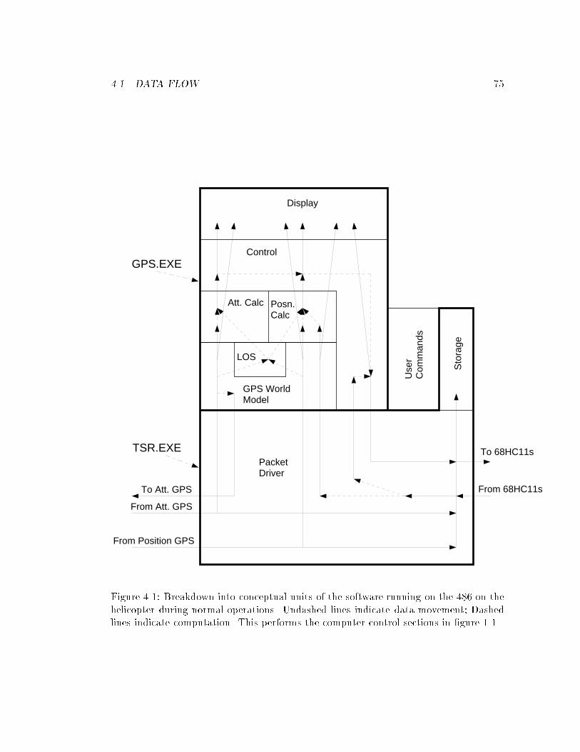
4.1. DATA FLOW 75
Sto
rage
Use
rC
omm
ands
GPS WorldModel
Att. Calc Posn.Calc
Display
Control
PacketDriver
To 68HC11s
From 68HC11s
From Position GPS
To Att. GPS
From Att. GPS
GPS.EXE
TSR.EXE
LOS
Figure 4.1: Breakdown into conceptual units of the software running on the 486 on thehelicopter during normal operations. Undashed lines indicate data movement; Dashedlines indicate computation. This performs the computer control sections in �gure 1.1.
76 CHAPTER 4. SOFTWARE
data structure, given the grand title of GPS World Model, which performs various
sanity checks to detect badly corrupted packets, maintains a history and synchronises
the phase measurements from the helicopter and ground position receivers. The GPS
World Model conceptual section also sends responses back to the Attitude GPS receiver
to manage the integer valid ags1.
The GPS position and attitude determination algorithms require knowledge of the
line of sight (LOS) vectors (s) to the satellites. There is conceptually a portion of the
GPS World model that accepts LOS vector packets2 from the two helicopter receivers3,
checks to see that they are sane, and then uses a history to interpolate or extrapolate
to obtain an LOS vector for each satellite in view for the current time.
Sitting on top of the GPS World model and LOS calculation stages are the imple-
mentations of the GPS algorithms given in chapter 2.
The attitude calculation algorithm is invoked each time that a new raw phase packet
comes from the attitude GPS receiver. The attitude calculation unit checks to see if the
integers have already been calculated. If not, this unit checks to see if there has been
su�cient phase change in the recent history to make an assumption of the existence of
signi�cant angular motion reasonable. If there is su�cient phase change, then the integer
resolution algorithm (section 2.4.2) is attempted. If the cost function (equation 2.54) is
small enough at the calculated minimum, and if the estimated integers are close enough
to mathematical integers, then the integers are assumed correct and remembered.
If the attitude integers are known, then the attitude computation conceptual unit
calculates the actual attitude and feeds roll, pitch and yaw up to the control system. If
the error in equation (2.17) is higher than expected from noise, the integer corresponding
1Instead of sending out a packet (which may be lost) to indicate a cycle slip, the attitude receiversends out a \phase valid" signal on each packet. The 486 then responds with a packet, saying that ithas noticed that the integer is not valid. The attitude receiver may then indicate that the integer valid ag is set. This will remain set until a cycle slip is detected (rare) or until visibility to the satellite hasbeen lost. The position receivers take the simpler route of sending out a cycle slip ag, and assumingthat packets will not be lost or that the 486 will be able to detect errors some other way. The positionreceivers need no feedback from the 486 during normal operation.
2The receivers use pseudorange to determine their position su�ciently accurately for the calculationof very accurate LOS vectors from the known satellite orbits.
3The base station does not send up LOS vectors, as it would be a waste of bandwidth over the radiolink.
4.1. DATA FLOW 77
to the worst �t to equation (2.53) is declared invalid. If new satellites have come into
view or an integer has been previously invalidated, the attitude calculation unit attempts
to determine the integer based upon the just-computed attitude. This allows satellites
to enter and leave visibility cleanly.
The position calculation conceptual unit is invoked whenever a pair of packets from
the base-station and the GPS position receiver arrive with matching time stamps. If
at least four satellites are visible on both the helicopter and base-station antennas, and
the corresponding integers are known, then the algorithm in section 2.3.2 is applied.
The solution (x; y; z) is passed up to the control level, and is also used to determine the
integers for new satellites that have come into view.
If at least one but fewer than four satellites are in view, and the corresponding
integers are known, then there is a signi�cant problem, as this corresponds to the case
of the helicopter having previously been ying along happily receiving at least four
satellites, and then losing su�cient satellites to compute position. In the hope that this
situation is temporary, an attempt to keep track of position is made by assuming that
one or more4 of the position variables x; y; z remain constant. This is not a marvelous
solution, but it can cope with small outages while the helicopter is under manual control.
This could in time be recovered from totally through the algorithm given in section 2.4.1.
If position integers are not believed known, and there are fewer than four satellites
visible, then nothing is done. If there are at least four satellites in view, then the integers
are estimated as if the base-station and helicopter antennas are colocated, as discussed
in section 2.4.1.
There are three inputs to the control conceptual unit during normal operations: the
position and attitude from the just-mentioned calculations, and the console values from
the pilot sent up from the packet driver. Whenever one of these changes, the control
unit calculates new control values and sends these commanded values back to the packet
driver, which packages them up and sends them o� to the 68HC11s and to the storage
area of memory for later down-loading.
4Four minus the number of satellites visible
78 CHAPTER 4. SOFTWARE
Above everything is a display which consists of a video display if connected5 and
some status LEDs on the parallel port if connected6.
The ground GPS operation can be considered as largely a subset of the above op-
eration as shown in �gure 4.2. The packet driver only has to deal with input from the
one position GPS receiver, and has the main job of sending the data from the GPS
receiver straight back out another serial line to the radio transmitter to be sent up to
the helicopter.
The packet driver can also save the GPS packets if required, and can send the packets
to a display module which can be very useful as a ground diagnostic to check that the
ground station is working properly and that there are su�cient satellites in view.
The 68HC11s have the basic functions of passing a data stream between the 486 on
the helicopter and the data radio (horizontal lines in �gure 4.3), and of passing servo
commands between the radio console and the servos (vertical lines in �gure 4.3). The
68HC11s also allow data to cross couple; the pilot's commands are inserted into the data
stream sent to the 486, and computer commanded values from the 486 are extracted out
of the data stream from the 486, and may be sent to the slave 486 { depending upon
the value of a switch set by the pilot { and transmitted as one of the servo values to the
master 68HC11.
Since the data coming from the data radio is position phases, and it is thus necessary
for this information to arrive at the 486 as quickly as possible, it is necessary for this
data to pass through the 68HC11s as quickly as possible.
4.1.2 Initialisation
Each GPS receiver needs to be initialised to send out the correct types of data at
the correct rate. This initialisation is the only data that ever needs to be sent to the
position GPS receivers. On the helicopter, this is automatically set up to occur when
the helicopter 486 boots up and starts running the ight software7. On the ground
5This is very useful for debugging, but is not actually on the helicopter. The computation programcan run on any 486 PC with suitable serial ports, and was developed and tested with the aid of acomputer monitor.
6This is actually on the helicopter7GPS.EXE
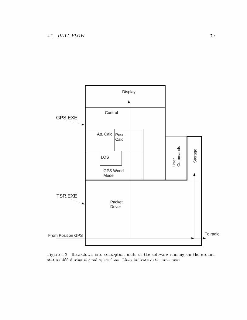
4.1. DATA FLOW 79
Sto
rage
Use
rC
omm
ands
GPS WorldModel
Att. Calc Posn.Calc
Display
Control
PacketDriver
To radioFrom Position GPS
GPS.EXE
TSR.EXE
LOS
Figure 4.2: Breakdown into conceptual units of the software running on the groundstation 486 during normal operations. Lines indicate data movement
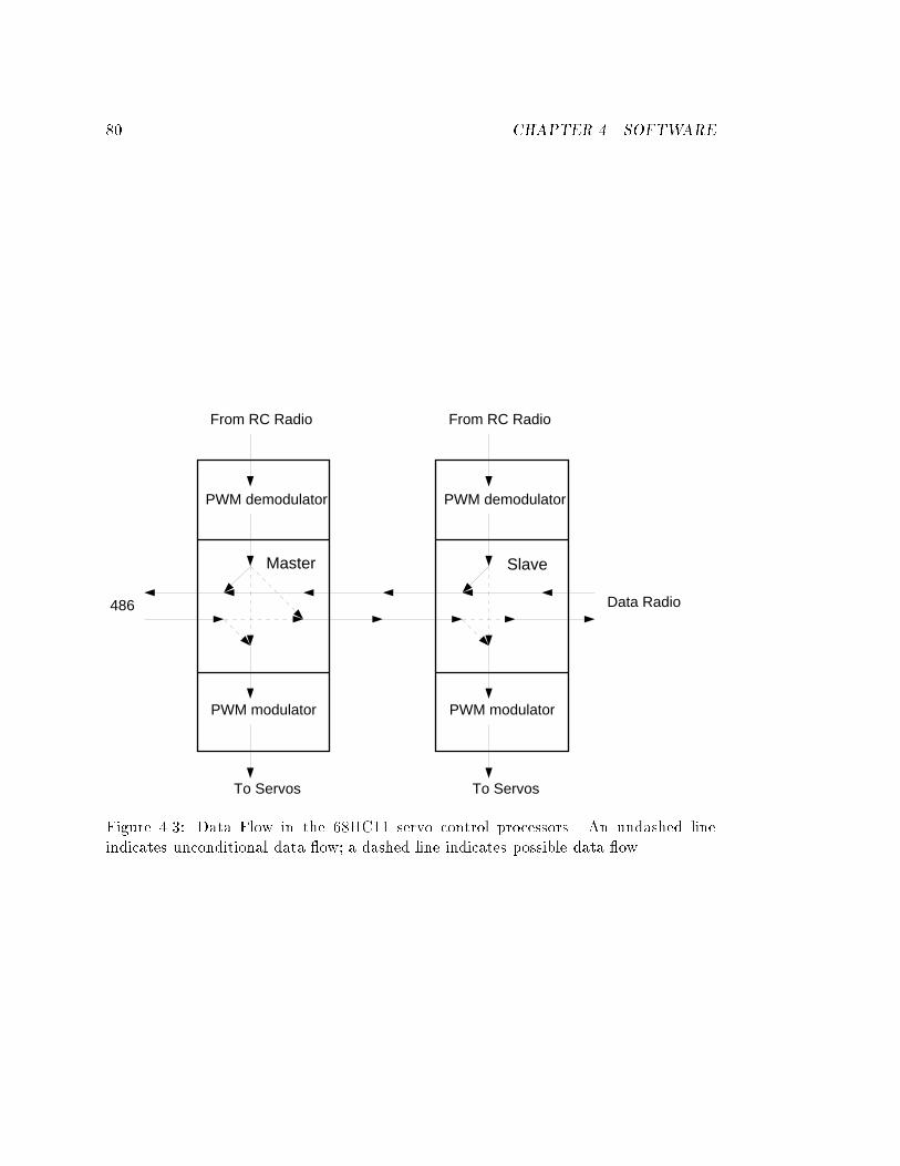
80 CHAPTER 4. SOFTWARE
PWM demodulator
PWM modulator
From RC Radio
To Servos
PWM demodulator
PWM modulator
From RC Radio
To Servos
Master Slave
Data Radio486
Figure 4.3: Data Flow in the 68HC11 servo control processors. An undashed lineindicates unconditional data ow; a dashed line indicates possible data ow.
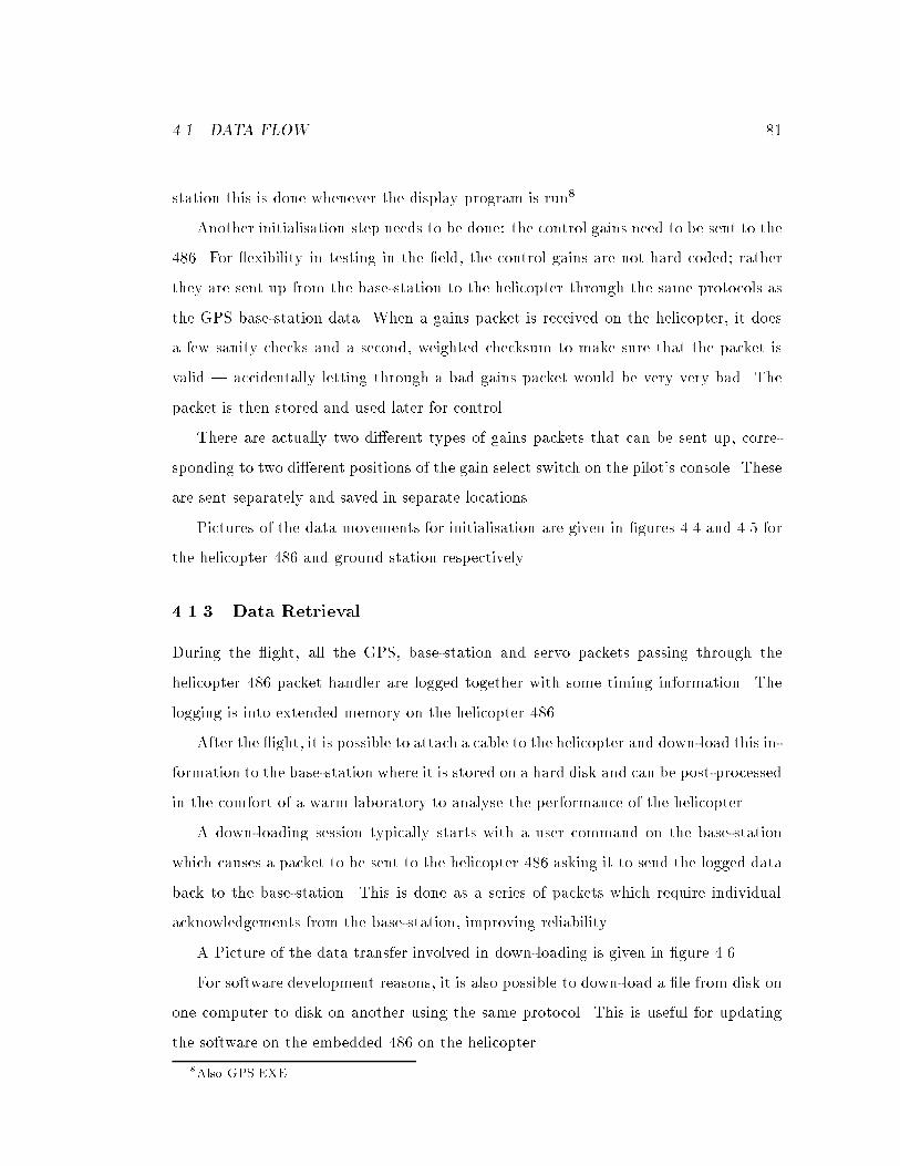
4.1. DATA FLOW 81
station this is done whenever the display program is run8.
Another initialisation step needs to be done: the control gains need to be sent to the
486. For exibility in testing in the �eld, the control gains are not hard coded; rather
they are sent up from the base-station to the helicopter through the same protocols as
the GPS base-station data. When a gains packet is received on the helicopter, it does
a few sanity checks and a second, weighted checksum to make sure that the packet is
valid | accidentally letting through a bad gains packet would be very very bad. The
packet is then stored and used later for control.
There are actually two di�erent types of gains packets that can be sent up, corre-
sponding to two di�erent positions of the gain select switch on the pilot's console. These
are sent separately and saved in separate locations.
Pictures of the data movements for initialisation are given in �gures 4.4 and 4.5 for
the helicopter 486 and ground station respectively.
4.1.3 Data Retrieval
During the ight, all the GPS, base-station and servo packets passing through the
helicopter 486 packet handler are logged together with some timing information. The
logging is into extended memory on the helicopter 486.
After the ight, it is possible to attach a cable to the helicopter and down-load this in-
formation to the base-station where it is stored on a hard disk and can be post-processed
in the comfort of a warm laboratory to analyse the performance of the helicopter.
A down-loading session typically starts with a user command on the base-station
which causes a packet to be sent to the helicopter 486 asking it to send the logged data
back to the base-station. This is done as a series of packets which require individual
acknowledgements from the base-station, improving reliability.
A Picture of the data transfer involved in down-loading is given in �gure 4.6
For software development reasons, it is also possible to down-load a �le from disk on
one computer to disk on another using the same protocol. This is useful for updating
the software on the embedded 486 on the helicopter.
8Also GPS.EXE
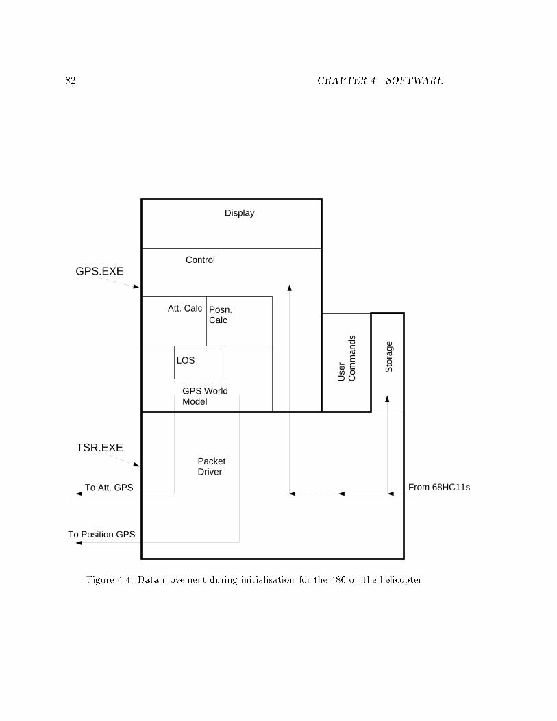
82 CHAPTER 4. SOFTWARE
Sto
rage
Use
rC
omm
ands
GPS WorldModel
Att. Calc Posn.Calc
Display
Control
PacketDriver
From 68HC11s
To Position GPS
To Att. GPS
GPS.EXE
TSR.EXE
LOS
Figure 4.4: Data movement during initialisation for the 486 on the helicopter
4.1. DATA FLOW 83
Sto
rage
Use
rC
omm
ands
GPS WorldModel
Att. Calc Posn.Calc
Display
Control
PacketDriver
To radio
GPS.EXE
TSR.EXE
LOS
REMOTE.EXE
To GPS Receiver
Figure 4.5: Data movement during initialisation for the ground-station
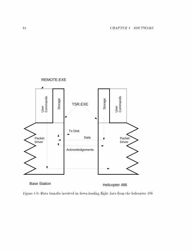
84 CHAPTER 4. SOFTWARE
Sto
rage
Use
rC
omm
ands
PacketDriver
REMOTE.EXE
Sto
rage
Use
rC
omm
ands
PacketDriver
To Disk
Data
Acknowledgements
TSR.EXE
Base Station Helicopter 486
Figure 4.6: Data transfer involved in down-loading ight data from the helicopter 486.
4.2. 68HC11 PROGRAMS 85
4.1.4 Post-processing
Rather than log the calculated positions and attitudes, all the GPS raw data is logged.
This enables one to study the behaviour of the sensor in more detail and study the
e�ects of changes in algorithms, as well as generating plots like �gure 2.7.
In order to reduce the possibility for errors, exactly the same GPS software is used
to postprocess the raw GPS data as is used on the helicopter.
The data can be replayed with the current software in two ways. One way is to replay
the data in real time, quantised to 1=18:2 second time intervals; the other method is to
send packets to the GPS program one packet at a time, sending a new packet as soon
as the current packet has been fully dealt with. This latter approach has the advantage
of being signi�cantly faster and generally more convenient.
The results of the processing are saved to �les by checking MS DOS environment
variables when an interesting value has been calculated to see whether that value should
be saved to a �le somewhere. This means that the only di�erence between the post-
processing setup and the helicopter is a few environment variables and the existence of
the video display.
A drawing of data transfer pathways during post processing is given in �gure 4.7.
Note how close this is to �gure 4.1.
The graphs in chapter 5 were generated using this method.
4.2 68HC11 programs
The 68HC11 programs are written in assembly language for e�ciency, and are almost
entirely interrupt driven. For low propagation delay reasons, the 68HC11s do not process
the packet structure of the incoming serial stream, but rather pass the data straight
through unless the data contains information intended for the 68HC11 as indicated by
the meta-packet structure described in section B.5.2.
The same meta-packet structure is used to insert the pilot's servo command values
into the serial stream at a nominal rate of 30Hz. This data rate could drop if the
serial link utilisation is so high that the transmit bu�er has not cleared since the last
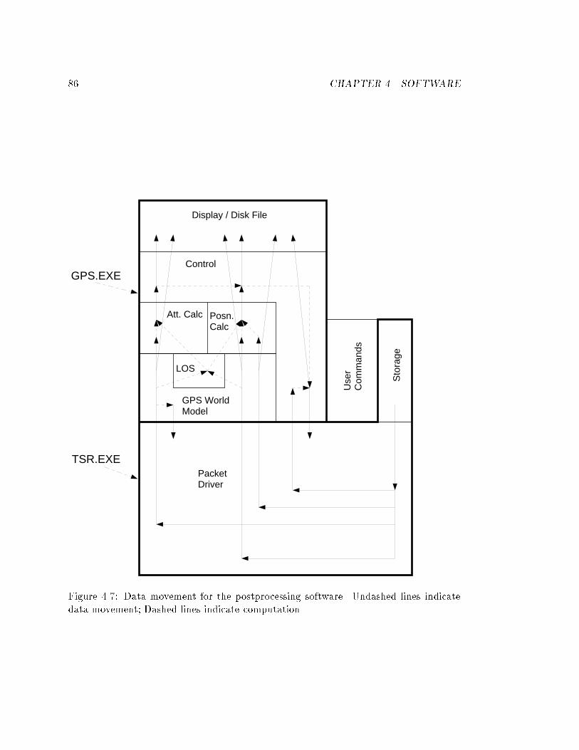
86 CHAPTER 4. SOFTWARE
Sto
rage
Use
rC
omm
ands
GPS WorldModel
Att. Calc Posn.Calc
Display / Disk File
Control
PacketDriver
GPS.EXE
TSR.EXE
LOS
Figure 4.7: Data movement for the postprocessing software. Undashed lines indicatedata movement; Dashed lines indicate computation.
4.3. 486 SOFTWARE 87
servo command packet. This feature prevents the GPS packets from being slowed down
more than about twelve milliseconds due to passing through the 68HC11s. Normally,
the servo commands take about thirty percent of the available bandwidth and the GPS
packets take up about �fty percent of the available bandwidth. The bandwidth required
by the GPS packets can increase temporarily when a pseudo-range position packet is
transmitted.
This software is quite simple, and has been tested extensively for reliability as the
ability to switch to manual control is vital for the safety of the helicopter.
This software is described in detail in section C.4.
4.3 486 software
There are potentially �ve logically distinct 486 computers mentioned above:
� The 486 on the helicopter
� The base station
� The down-load computer
� The post-processing/analysis computer
� The development environment
In practice, these jobs are shared among a smaller number of computers, but there are
�ve separate tasks to be done, requiring di�erent, but related, software. Coping with
the immense software engineering task of maintaining �ve separate versions of the one
set of software seemed worth avoiding. Thus, as alluded to in section 4.1.4, a decision
was made to use just one set of software with a general architecture on each of those
�ve logical machines. The only distinction between the software is in external command
line options or environment variables.
As can be seen in the previous �gures in this chapter showing the breakdown of the
various software processes into conceptual units and data movement, the architecture
of each mode is very similar, making this scheme feasible and e�cient.
88 CHAPTER 4. SOFTWARE
Having made that decision, it was then decided to break the software that runs on
the 486 computers into three main programs.
The lowest level program, TSR.EXE contains the packet driver and the data storage
previously discussed. TSR.EXE also manages timings, �le transfers, console emulation,
and some other useful utilities for using an embedded processor. A detailed description
of TSR.EXE is given in appendix B. This program contains most of the IBM PC hardware
speci�c operations, making the rest of the software more convenient to develop.
On all computers, TSR.EXE runs in the background, and other programs communi-
cate to in by
� Giving it a command like \Down-load ight data from the remote machine"
� Explicitly sending a packet, such as GPS initialisation to some logical unit (such
as the attitude GPS board).
� Being given a packet from some logical unit (such as the remote GPS position
receiver).
TSR.EXE takes care of physical to logical port mappings, baud rates, and other commu-
nication parameters for di�erent setups through command line parameters. TSR.EXE
can also be set up to automatically retransmit certain GPS packets, functioning as the
base-station in the background.
On top of this sits one of two application programs. The smaller, REMOTE.EXE
allows a user to send commands directly to TSR.EXE like \Down-load ight data from
the remote machine" or \Send the following gains to the helicopter." Details are given
in section B.6.2.
GPS.EXE is the most complex. It contains
� The GPS World Model, which is responsible for initialising the GPS receivers,
maintaining the attitude integers and sychronising data. This includes the Line
of Sight unit.
� Position Computation, responsible for initialising the GPS position integers and
computing three dimensional position.
4.4. CONTROL 89
� Attitude Computation, responsible for initialising the GPS attitude integers and
computing the three attitude degrees of freedom
� Control, which takes the pilot's console commands and the six position and atti-
tude values and computes servo commands
� Display, which shows what is going on in the system on a video monitor, either as
text or a graphical representation of the helicopter's current position and orienta-
tion. File output from post-processing can be considered part of this unit.
GPS.EXE is designed to work in real time, always processing the most recent data as
soon as it can to get as low data delay from computation as possible. Of the algorithms
in chapter 2, position determination is the fastest, running in a couple of milliseconds
maximum. Most of the execution time is getting the right data in the right place. The
attitude determination can be fairly slow, depending upon the data. Taking longer than
50 milliseconds is unusual. The really slow algorithm is the attitude integer resolution,
which may take almost a second. Fortunately this typically only has to be performed
once, although GPS.EXE continues responding to other GPS tasks (such as position
computation) whilst attitude integer resolution is taking place. This is important if the
helicopter is regaining attitude integers in the air through large angular motions which
are likely to cause satellite loss and recovery at the position receiver.
For postprocessing, the same program GPS.EXE is used, taking as argument the name
of the �le containing ight data downloaded at the end of a ight. This data is then
processed as if the packets were being received again. By saving various computations
(such as position) to a disk �le the downloaded information can be analysed.
4.4 Control
The control system used was a very primitive one, relying on a very simplistic model of
the helicopter with no cross coupling between degrees of freedom, and feedback loops
based on �gure 1.1.
In actuality the cross coupling can take several forms such as
90 CHAPTER 4. SOFTWARE
� Coupling from controls : Increasing thrust increases torque on the main rotor and
causes a yaw motion
� Coupling from motion : Forwards velocity causes increased lift on the forward
moving blade and decreased lift on the backward moving blade, causing a roll
motion and overall increased lift.
� Coupling from sensor : The sensor is on the tail of the helicopter, so an angular
motion of the helicopter shows up as a translation.
� Coupling from biases : The biases due to trim settings are di�erent in the di�erent
axes of the helicopter. Thus a rotation will change the e�ective direction of the
trim o�sets, coupling into control commands.
The �rst two (and similar) e�ects could be compensated for with a good system
identi�cation and cross terms in the control law. Accounting for the displacement from
the tail to the center of mass can be performed as one has both position and attitude; it
was not done here as there was some doubt as to the e�ects of the noise coupled in from
the angular measurements, and the belief that this e�ect was small compared to other
ignored terms. The coupling from biases could be dealt with by an integral term in the
control loops. This was not done as the knowledge of the system is not particularly high,
and it was desired to obtain a stable system before adding a potentially destabilising
term.
As said before, these coupling terms were neglected, and e�ectively four PD con-
trollers were set up around the four statically controllable degrees of freedom: altitude,
heading, and forwards and transverse location.
These four control loops are presented with simplistic models of the plant in �gures
4.8 (altitude), 4.9 (heading), 4.10 (pitch/forward movement), and 4.11 (roll/transverse
movement).
The altitude control loop is the most straight forward both because it is the least
unstable9 and because the obvious solution of a PD controller using vertical position
9Steve (the pilot) could trim the throttle and leave it at a �xed value for an extended period of timewith the other three loops closed. All other loops required constant pilot feedback when not closed.
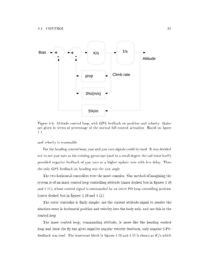
4.4. CONTROL 91
1/sK/s
prop
--+ +
Altitude
Climb rate
Bias
5%/m
3%/(m/s)
Figure 4.8: Altitude control loop, with GPS feedback on position and velocity. Gainsare given in terms of percentage of the normal full control actuation. Based on �gure1.1.
and velocity is reasonable.
For the heading control loop, yaw and yaw rate signals could be used. It was decided
not to use yaw rate as the existing gyroscope (and to a small degree the tail rotor itself)
provided negative feedback of yaw rate at a higher update rate with less delay. Thus
the only GPS feedback on heading was the yaw angle.
The two horizontal controllers were the most complex. One method of imagining the
system is of an inner control loop controlling attitude (inner dashed box in �gures 4.10
and 4.11), whose control signal is commanded by an outer PD loop controlling position
(outer dashed box in �gures 4.10 and 4.11).
The outer controller is fairly simple: use the current attitude signal to resolve the
absolute error in horizontal position and velocity into the body axis, and use this in the
control loop.
The inner control loop, commanding attitude, is more like the heading control
loop and since the y-bar gives negative angular velocity feedback, only angular GPS-
feedback was used. The innermost block in �gures 4.10 and 4.11 is shown as K=s which
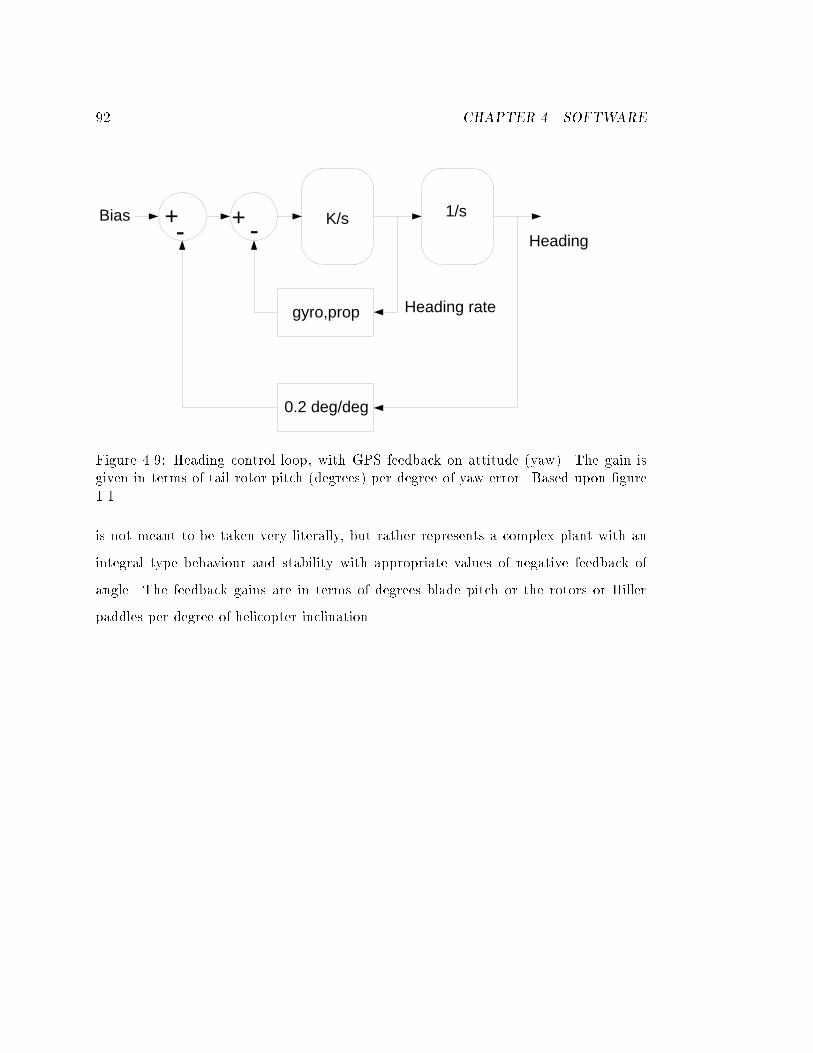
92 CHAPTER 4. SOFTWARE
1/sK/s
0.2 deg/deg
gyro,prop
--+ +
Heading
Heading rate
Bias
Figure 4.9: Heading control loop, with GPS feedback on attitude (yaw). The gain isgiven in terms of tail rotor pitch (degrees) per degree of yaw error. Based upon �gure1.1.
is not meant to be taken very literally, but rather represents a complex plant with an
integral type behaviour and stability with appropriate values of negative feedback of
angle. The feedback gains are in terms of degrees blade pitch or the rotors or Hiller
paddles per degree of helicopter inclination.
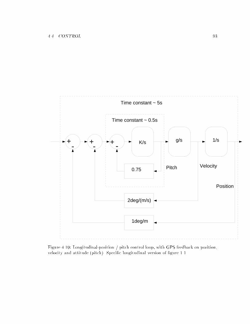
4.4. CONTROL 93
1/sg/sK/s
1deg/m
2deg/(m/s)
0.75
---+ + +
Pitch Velocity
Position
Time constant ~ 0.5s
Time constant ~ 5s
Figure 4.10: Longitudinal-position / pitch control loop, with GPS feedback on position,velocity and attitude (pitch). Speci�c longitudinal version of �gure 1.1.
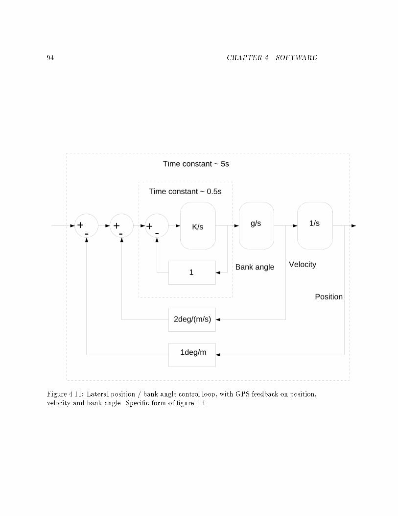
94 CHAPTER 4. SOFTWARE
1/sg/sK/s
1deg/m
2deg/(m/s)
1
---+ + +
Bank angle Velocity
Position
Time constant ~ 0.5s
Time constant ~ 5s
Figure 4.11: Lateral position / bank angle control loop, with GPS feedback on position,velocity and bank angle. Speci�c form of �gure 1.1.
Chapter 5
Flight-Test Results
The helicopter has own under autonomous closed-loop GPS control, has hovered stably,
and has shown an excellent ability to deal with command-induced transients on the
order of ten metres. Only GPS signals were used to control both helicopter location
and attitude.
Due to the signi�cant e�ort of setting up equipment for a ight, and troubles with
vibration causing unreliability, there have been to date only two ights with all loops
closed by GPS using the control gains given in �gures 4.8, 4.9, 4.10, and 4.11. This
chapter describes the results of these ights. The graphs in this chapter come from
GPS data down-loaded from the helicopter after the ights.
5.1 Flight Pro�le
A typical test ight is shown in �gure 5.1. The helicopter took o� (under manual
control), was own by the pilot (Steve Morris) up to a relatively safe high location, where
the computer control switch was thrown. The helicopter repositioned a few metres due
to the biasing errors in the zero-point trim adjustments, and then hovered autonomously
(\Hands o�"). After about a minute, Steve commanded some transients manually via
perturbations on the control console (which acts as a position control in computer mode)
to demonstrate the closed-loop system's transient recovery from disturbances. Lastly,
Steve put the helicopter back into manual mode and landed the helicopter, whence we
95
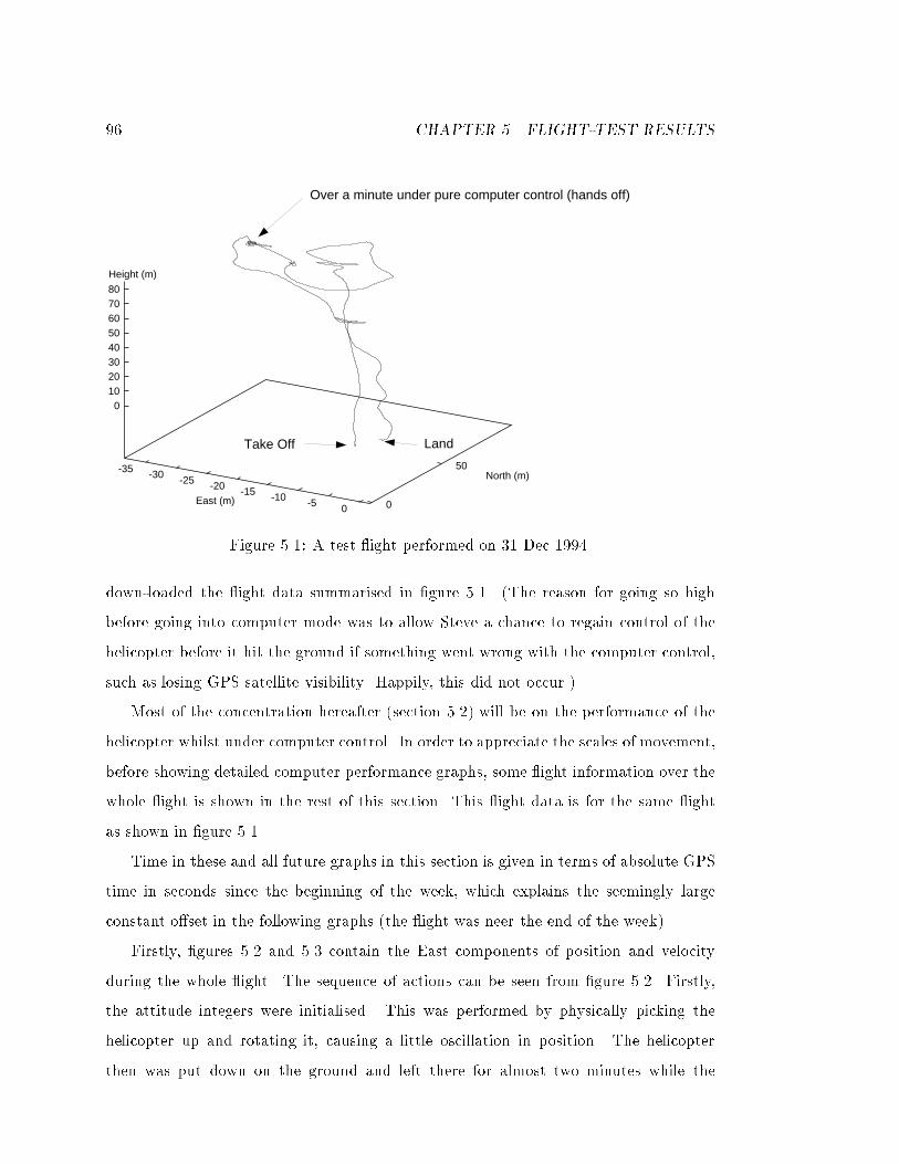
96 CHAPTER 5. FLIGHT-TEST RESULTS
-35 -30 -25 -20 -15 -10 -5 0 0
50
01020304050607080
East (m)
North (m)
Height (m)
Take Off Land
Over a minute under pure computer control (hands off)
Figure 5.1: A test ight performed on 31 Dec 1994.
down-loaded the ight data summarised in �gure 5.1. (The reason for going so high
before going into computer mode was to allow Steve a chance to regain control of the
helicopter before it hit the ground if something went wrong with the computer control,
such as losing GPS satellite visibility. Happily, this did not occur.)
Most of the concentration hereafter (section 5.2) will be on the performance of the
helicopter whilst under computer control. In order to appreciate the scales of movement,
before showing detailed computer performance graphs, some ight information over the
whole ight is shown in the rest of this section. This ight data is for the same ight
as shown in �gure 5.1.
Time in these and all future graphs in this section is given in terms of absolute GPS
time in seconds since the beginning of the week, which explains the seemingly large
constant o�set in the following graphs (the ight was neer the end of the week).
Firstly, �gures 5.2 and 5.3 contain the East components of position and velocity
during the whole ight. The sequence of actions can be seen from �gure 5.2. Firstly,
the attitude integers were initialised. This was performed by physically picking the
helicopter up and rotating it, causing a little oscillation in position. The helicopter
then was put down on the ground and left there for almost two minutes while the
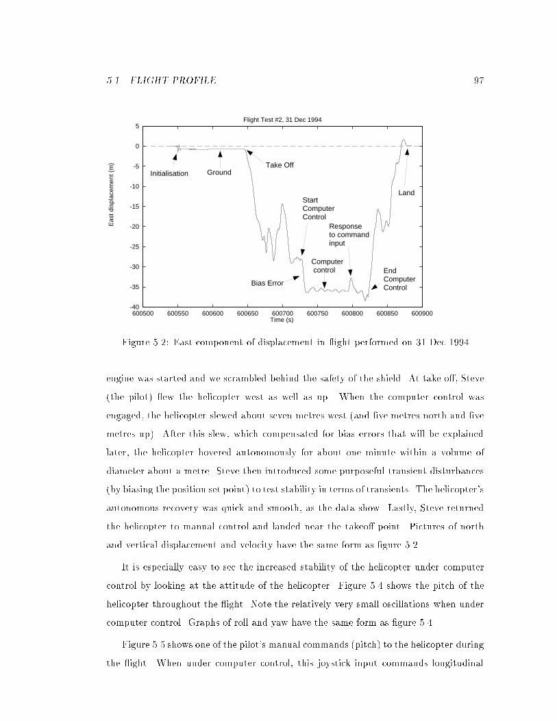
5.1. FLIGHT PROFILE 97
-40
-35
-30
-25
-20
-15
-10
-5
0
5
600500 600550 600600 600650 600700 600750 600800 600850 600900
Eas
t dis
plac
emen
t (m
)
Time (s)
Flight Test #2, 31 Dec 1994
InitialisationTake Off
Computer control
Response to commandinput
Ground
Land
Bias Error
EndComputerControl
StartComputerControl
Figure 5.2: East component of displacement in ight performed on 31 Dec 1994
engine was started and we scrambled behind the safety of the shield. At take o�, Steve
(the pilot) ew the helicopter west as well as up. When the computer control was
engaged, the helicopter slewed about seven metres west (and �ve metres north and �ve
metres up). After this slew, which compensated for bias errors that will be explained
later, the helicopter hovered autonomously for about one minute within a volume of
diameter about a metre. Steve then introduced some purposeful transient disturbances
(by biasing the position set point) to test stability in terms of transients. The helicopter's
autonomous recovery was quick and smooth, as the data show. Lastly, Steve returned
the helicopter to manual control and landed near the takeo� point. Pictures of north
and vertical displacement and velocity have the same form as �gure 5.2.
It is especially easy to see the increased stability of the helicopter under computer
control by looking at the attitude of the helicopter. Figure 5.4 shows the pitch of the
helicopter throughout the ight. Note the relatively very small oscillations when under
computer control. Graphs of roll and yaw have the same form as �gure 5.4.
Figure 5.5 shows one of the pilot's manual commands (pitch) to the helicopter during
the ight. When under computer control, this joystick input commands longitudinal
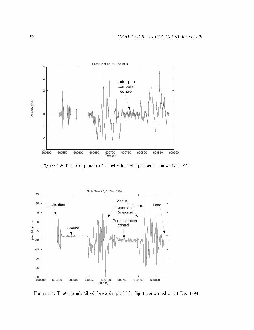
98 CHAPTER 5. FLIGHT-TEST RESULTS
-3
-2
-1
0
1
2
3
4
600500 600550 600600 600650 600700 600750 600800 600850 600900
Vel
ocity
(m
/s)
Time (s)
Flight Test #2, 31 Dec 1994
under purecomputer
control
Figure 5.3: East component of velocity in ight performed on 31 Dec 1994
-30
-25
-20
-15
-10
-5
0
5
10
15
600500 600550 600600 600650 600700 600750 600800 600850
pitc
h (d
egre
es)
time (s)
Flight Test #2, 31 Dec 1994
Initialisation
Ground
Manual
Pure computer control
LandCommandResponse
Figure 5.4: Theta (angle tilted forwards, pitch) in ight performed on 31 Dec 1994
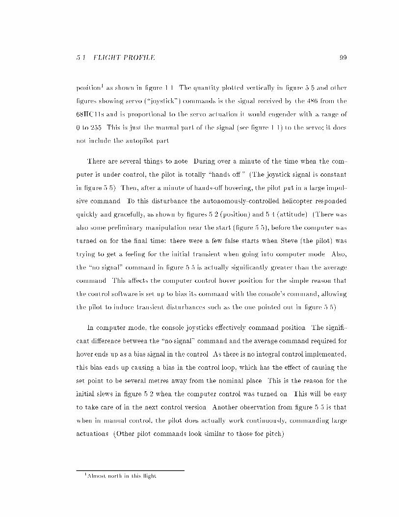
5.1. FLIGHT PROFILE 99
position1 as shown in �gure 1.1. The quantity plotted vertically in �gure 5.5 and other
�gures showing servo (\joystick") commands is the signal received by the 486 from the
68HC11s and is proportional to the servo actuation it would engender with a range of
0 to 255. This is just the manual part of the signal (see �gure 1.1) to the servo; it does
not include the autopilot part.
There are several things to note. During over a minute of the time when the com-
puter is under control, the pilot is totally \hands o�." (The joystick signal is constant
in �gure 5.5). Then, after a minute of hands-o� hovering, the pilot put in a large impul-
sive command. To this disturbance the autonomously-controlled helicopter responded
quickly and gracefully, as shown by �gures 5.2 (position) and 5.4 (attitude). (There was
also some preliminary manipulation near the start (�gure 5.5), before the computer was
turned on for the �nal time: there were a few false starts when Steve (the pilot) was
trying to get a feeling for the initial transient when going into computer mode. Also,
the \no signal" command in �gure 5.5 is actually signi�cantly greater than the average
command. This a�ects the computer control hover position for the simple reason that
the control software is set up to bias its command with the console's command, allowing
the pilot to induce transient disturbances such as the one pointed out in �gure 5.5).
In computer mode, the console joysticks e�ectively command position. The signi�-
cant di�erence between the \no signal" command and the average command required for
hover ends up as a bias signal in the control. As there is no integral control implemented,
this bias ends up causing a bias in the control loop, which has the e�ect of causing the
set point to be several metres away from the nominal place. This is the reason for the
initial slews in �gure 5.2 when the computer control was turned on. This will be easy
to take care of in the next control version. Another observation from �gure 5.5 is that
when in manual control, the pilot does actually work continuously, commanding large
actuations. (Other pilot commands look similar to those for pitch).
1Almost north in this ight.
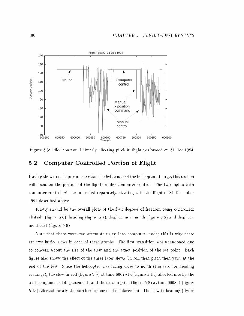
100 CHAPTER 5. FLIGHT-TEST RESULTS
50
60
70
80
90
100
110
120
130
140
600500 600550 600600 600650 600700 600750 600800 600850 600900
Joys
tick
posi
tion
Time (s)
Flight Test #2, 31 Dec 1994
Ground Computer control
Manualcontrol
Manualx positioncommand
Figure 5.5: Pilot command directly a�ecting pitch in ight performed on 31 Dec 1994
5.2 Computer Controlled Portion of Flight
Having shown in the previous section the behaviour of the helicopter at large, this section
will focus on the portion of the ights under computer control. The two ights with
computer control will be presented separately, starting with the ight of 31 December
1994 described above.
Firstly should be the overall plots of the four degrees of freedom being controlled:
altitude (�gure 5.6), heading (�gure 5.7), displacement north (�gure 5.8) and displace-
ment east (�gure 5.9).
Note that there were two attempts to go into computer mode; this is why there
are two initial slews in each of these graphs. The �rst transition was abandoned due
to concern about the size of the slew and the exact position of the set point. Each
�gure also shows the e�ect of the three later slews (in roll then pitch then yaw) at the
end of the test. Since the helicopter was facing close to north (the zero for heading
readings), the slew in roll (�gure 5.9) at time 600794 s (�gure 5.14) a�ected mostly the
east component of displacement, and the slew in pitch (�gure 5.8) at time 600801 (�gure
5.13) a�ected mostly the north component of displacement. The slew in heading (�gure
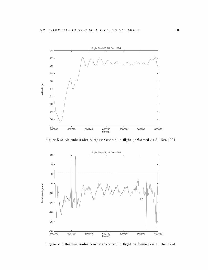
5.2. COMPUTER CONTROLLED PORTION OF FLIGHT 101
54
56
58
60
62
64
66
68
70
72
74
600700 600720 600740 600760 600780 600800 600820
Alti
tude
(m
)
time (s)
Flight Test #2, 31 Dec 1994
Figure 5.6: Altitude under computer control in ight performed on 31 Dec 1994
-30
-25
-20
-15
-10
-5
0
5
10
600700 600720 600740 600760 600780 600800 600820
head
ing
(deg
rees
)
time (s)
Flight Test #2, 31 Dec 1994
Figure 5.7: Heading under computer control in ight performed on 31 Dec 1994
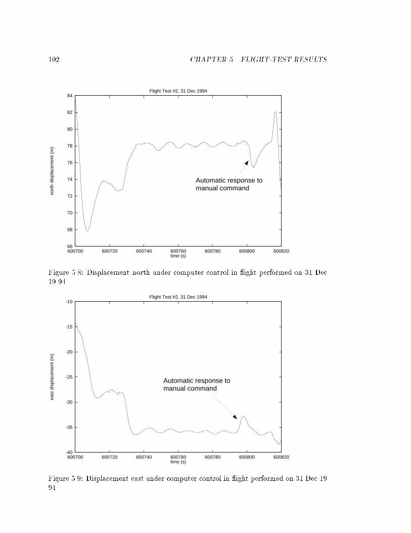
102 CHAPTER 5. FLIGHT-TEST RESULTS
66
68
70
72
74
76
78
80
82
84
600700 600720 600740 600760 600780 600800 600820
nort
h di
spla
cem
ent (
m)
time (s)
Flight Test #2, 31 Dec 1994
Automatic response tomanual command
Figure 5.8: Displacement north under computer control in ight performed on 31 Dec19 94
-40
-35
-30
-25
-20
-15
-10
600700 600720 600740 600760 600780 600800 600820
east
dis
plac
emen
t (m
)
time (s)
Flight Test #2, 31 Dec 1994
Automatic response tomanual command
Figure 5.9: Displacement east under computer control in ight performed on 31 Dec 1994
5.2. COMPUTER CONTROLLED PORTION OF FLIGHT 103
5.7) at time 600805 (�gure 5.12) a�ected slightly both horizontal displacements, as the
point on the helicopter being measured was the tail antenna, which intrinsically couples
rotation into position (as mentioned in section 4.4).
A distinctive pattern about these graphs is the oscillation that continues after the
initial transients have well died away. This oscillation occurs with the same roughly
eleven-second period in all four degrees of freedom, linked through the cross couplings
as mentioned in section 4.4. (From the data, the horizontal motion is along a northeast-
southwest line). The limit-cycle behaviour probably came from the delays in the system
and/or or the quantization of the servos. The servos were quantised to a motion of
about a third of a degree, which corresponds to a displacement of about a foot with the
current gains, which is comparable to the size of the limit cycle.
The period of this limit cycle can be determined formally by performing an auto-
correlation of one variable with respect to a time delay. Figure 5.10 contains an auto-
correlation of the � (roll) signal over the time period (600740,600790). This indicates
that the period of the limit cycle is eleven seconds.
The pilot commands that were put in just at the beginning and again at the end of
this period of totally autonomous ight are given in �gures 5.11, 5.12, 5.13 and 5.14.
Again, from �gure 1.1, since the system is still under automatic control, the manual
inputs are commands in lateral position, forward position, altitude and heading. One
can see in these graphs the y position impulse at time 600793 s, the x position impulse
at time 600802 s and the heading impulse at time 600805 s. The autonomous system's
response to these impulses can be seen in �gures 5.9, 5.8 and 5.7 respectively.
After answering the obvious questions of \Is it stable?" (yes) and \Is there a limit
cycle?" (yes), comes the question \How fast is the response to a slew command, and how
does this compare to the expected behaviour based on the control system and model
used?"
Fortunately the o�set biases which cause the actual set point to be several metres
away from the expected hover point (where the helicopter was when the computer control
switch was thrown) give excellent slews, as they represent a true step function input to
the control system. It is unfortunate that they are all simultaneous, which could cause
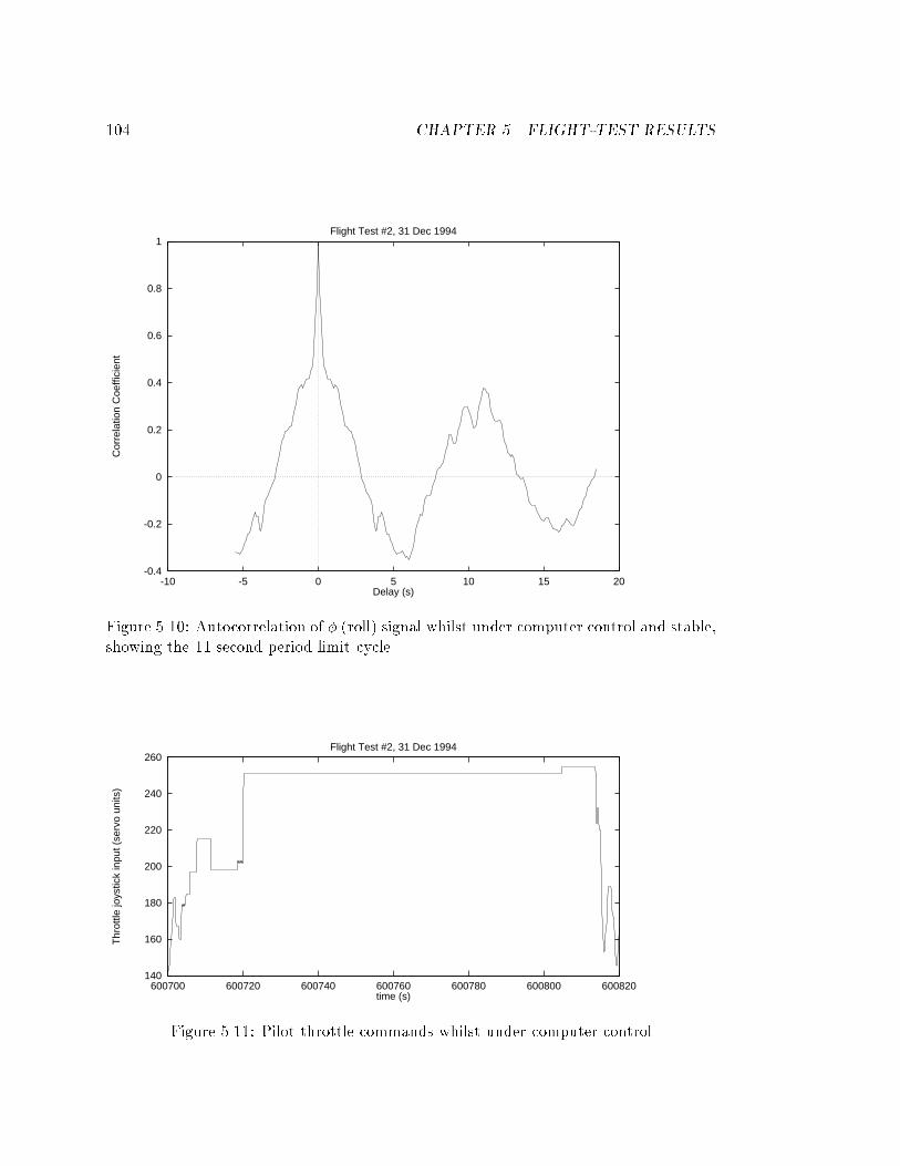
104 CHAPTER 5. FLIGHT-TEST RESULTS
-0.4
-0.2
0
0.2
0.4
0.6
0.8
1
-10 -5 0 5 10 15 20
Cor
rela
tion
Coe
ffici
ent
Delay (s)
Flight Test #2, 31 Dec 1994
Figure 5.10: Autocorrelation of � (roll) signal whilst under computer control and stable,showing the 11 second period limit cycle.
140
160
180
200
220
240
260
600700 600720 600740 600760 600780 600800 600820
Thr
ottle
joys
tick
inpu
t (se
rvo
units
)
time (s)
Flight Test #2, 31 Dec 1994
Figure 5.11: Pilot throttle commands whilst under computer control
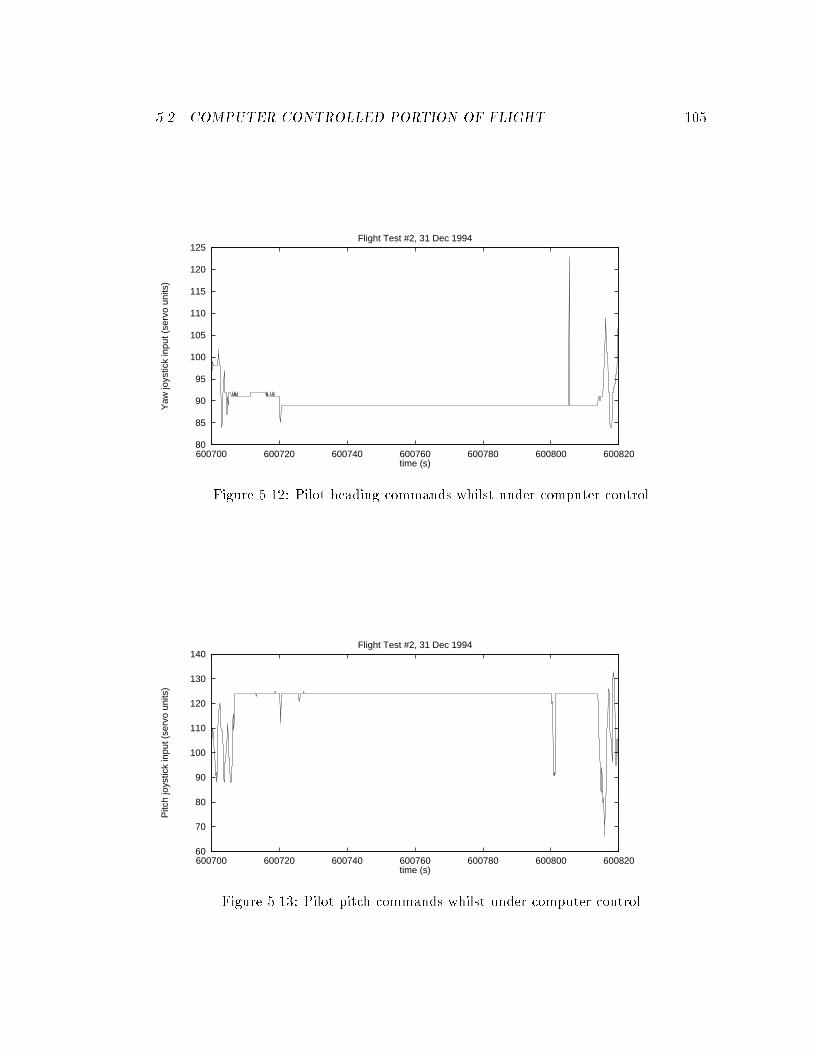
5.2. COMPUTER CONTROLLED PORTION OF FLIGHT 105
80
85
90
95
100
105
110
115
120
125
600700 600720 600740 600760 600780 600800 600820
Yaw
joys
tick
inpu
t (se
rvo
units
)
time (s)
Flight Test #2, 31 Dec 1994
Figure 5.12: Pilot heading commands whilst under computer control
60
70
80
90
100
110
120
130
140
600700 600720 600740 600760 600780 600800 600820
Pitc
h jo
ystic
k in
put (
serv
o un
its)
time (s)
Flight Test #2, 31 Dec 1994
Figure 5.13: Pilot pitch commands whilst under computer control
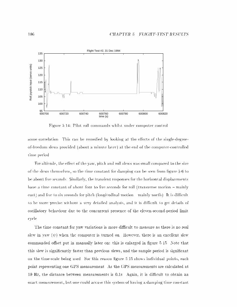
106 CHAPTER 5. FLIGHT-TEST RESULTS
95
100
105
110
115
120
125
130
135
600700 600720 600740 600760 600780 600800 600820
Rol
l joy
stic
k in
put (
serv
o un
its)
time (s)
Flight Test #2, 31 Dec 1994
Figure 5.14: Pilot roll commands whilst under computer control
some correlation. This can be remedied by looking at the e�ects of the single-degree-
of-freedom slews provided (about a minute later) at the end of the computer-controlled
time period.
For altitude, the e�ect of the yaw, pitch and roll slews was small compared to the size
of the slews themselves, so the time constant for damping can be seen from �gure 5.6 to
be about �ve seconds. Similarly, the transient responses for the horizontal displacements
have a time constant of about four to �ve seconds for roll (transverse motion { mainly
east) and �ve to six seconds for pitch (longitudinal motion { mainly north). It is di�cult
to be more precise without a very detailed analysis, and it is di�cult to get details of
oscillatory behaviour due to the concurrent presence of the eleven-second-period limit
cycle.
The time constant for yaw variations is more di�cult to measure as there is no real
slew in yaw ( ) when the computer is turned on. However, there is an excellent slew
commanded o�set put in manually later on: this is enlarged in �gure 5.15. Note that
this slew is signi�cantly faster than previous slews, and the sample period is signi�cant
on the time-scale being used. For this reason �gure 5.15 shows individual points, each
point representing one GPS measurement. As the GPS measurements are calculated at
10 Hz, the distance between measurements is 0:1s. Again, it is di�cult to obtain an
exact measurement, but one could accuse this system of having a damping time constant
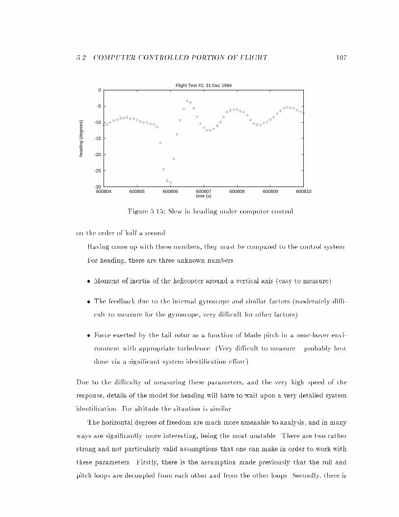
5.2. COMPUTER CONTROLLED PORTION OF FLIGHT 107
-30
-25
-20
-15
-10
-5
0
600804 600805 600806 600807 600808 600809 600810
head
ing
(deg
rees
)
time (s)
Flight Test #2, 31 Dec 1994
Figure 5.15: Slew in heading under computer control.
on the order of half a second.
Having come up with these numbers, they must be compared to the control system.
For heading, there are three unknown numbers
� Moment of inertia of the helicopter around a vertical axis (easy to measure)
� The feedback due to the internal gyroscope and similar factors (moderately di�-
cult to measure for the gyroscope, very di�cult for other factors)
� Force exerted by the tail rotor as a function of blade pitch in a near-hover envi-
ronment with appropriate turbulence. (Very di�cult to measure { probably best
done via a signi�cant system identi�cation e�ort).
Due to the di�culty of measuring these parameters, and the very high speed of the
response, details of the model for heading will have to wait upon a very detailed system
identi�cation. For altitude the situation is similar.
The horizontal degrees of freedom are much more amenable to analysis, and in many
ways are signi�cantly more interesting, being the most unstable. There are two rather
strong and not particularly valid assumptions that one can make in order to work with
these parameters. Firstly, there is the assumption made previously that the roll and
pitch loops are decoupled from each other and from the other loops. Secondly, there is
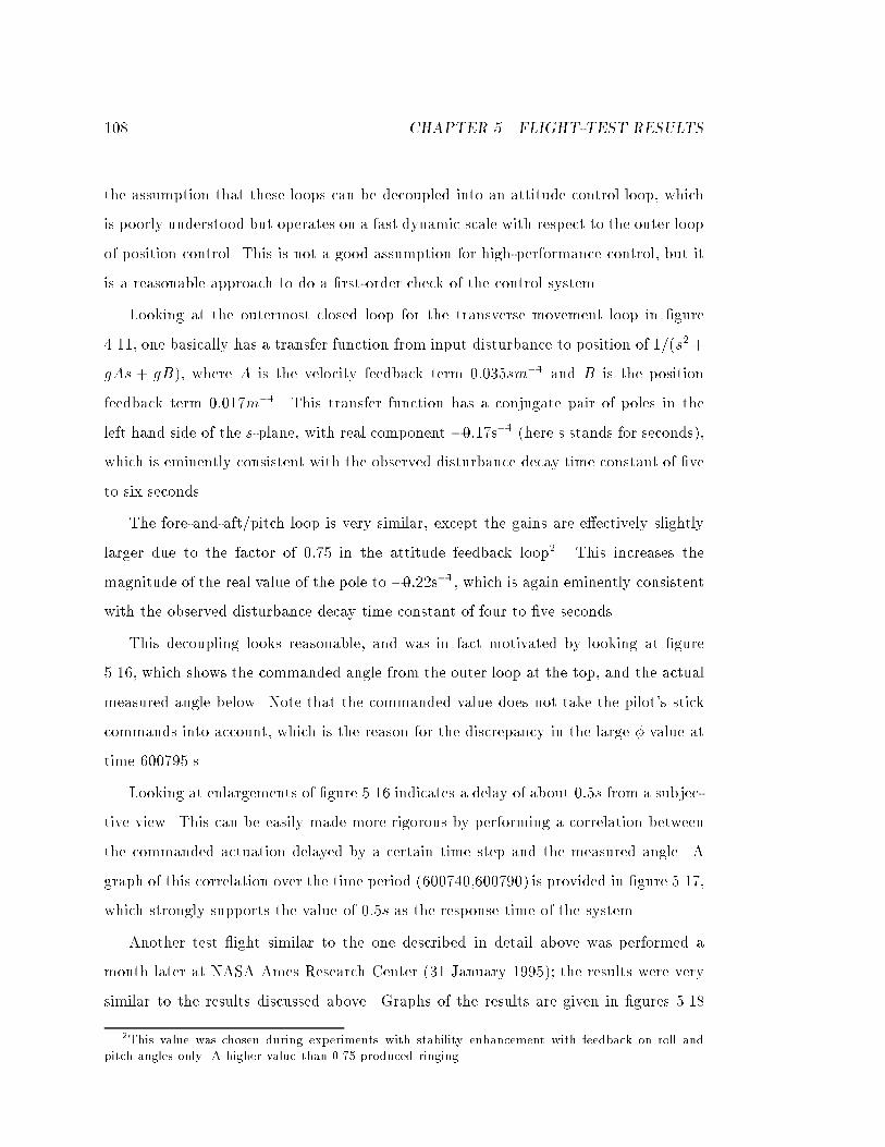
108 CHAPTER 5. FLIGHT-TEST RESULTS
the assumption that these loops can be decoupled into an attitude control loop, which
is poorly understood but operates on a fast dynamic scale with respect to the outer loop
of position control. This is not a good assumption for high-performance control, but it
is a reasonable approach to do a �rst-order check of the control system.
Looking at the outermost closed loop for the transverse movement loop in �gure
4.11, one basically has a transfer function from input disturbance to position of 1=(s2+
gAs + gB), where A is the velocity feedback term 0:035sm�1 and B is the position
feedback term 0:017m�1. This transfer function has a conjugate pair of poles in the
left hand side of the s-plane, with real component �0:17s�1 (here s stands for seconds),which is eminently consistent with the observed disturbance decay time constant of �ve
to six seconds.
The fore-and-aft/pitch loop is very similar, except the gains are e�ectively slightly
larger due to the factor of 0:75 in the attitude feedback loop2. This increases the
magnitude of the real value of the pole to �0:22s�1, which is again eminently consistent
with the observed disturbance decay time constant of four to �ve seconds.
This decoupling looks reasonable, and was in fact motivated by looking at �gure
5.16, which shows the commanded angle from the outer loop at the top, and the actual
measured angle below. Note that the commanded value does not take the pilot's stick
commands into account, which is the reason for the discrepancy in the large � value at
time 600795 s.
Looking at enlargements of �gure 5.16 indicates a delay of about 0:5s from a subjec-
tive view. This can be easily made more rigorous by performing a correlation between
the commanded actuation delayed by a certain time step and the measured angle. A
graph of this correlation over the time period (600740,600790) is provided in �gure 5.17,
which strongly supports the value of 0:5s as the response time of the system.
Another test ight similar to the one described in detail above was performed a
month later at NASA Ames Research Center (31 January 1995); the results were very
similar to the results discussed above. Graphs of the results are given in �gures 5.18
2This value was chosen during experiments with stability enhancement with feedback on roll andpitch angles only. A higher value than 0.75 produced ringing.
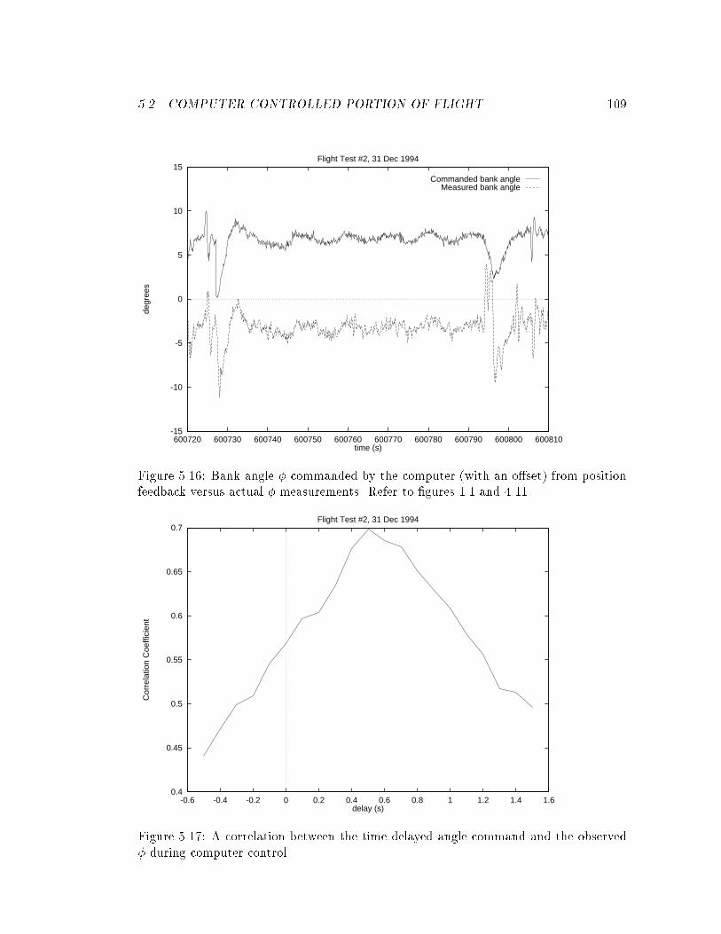
5.2. COMPUTER CONTROLLED PORTION OF FLIGHT 109
-15
-10
-5
0
5
10
15
600720 600730 600740 600750 600760 600770 600780 600790 600800 600810
degr
ees
time (s)
Flight Test #2, 31 Dec 1994
Commanded bank angleMeasured bank angle
Figure 5.16: Bank angle � commanded by the computer (with an o�set) from positionfeedback versus actual � measurements. Refer to �gures 1.1 and 4.11.
0.4
0.45
0.5
0.55
0.6
0.65
0.7
-0.6 -0.4 -0.2 0 0.2 0.4 0.6 0.8 1 1.2 1.4 1.6
Cor
rela
tion
Coe
ffici
ent
delay (s)
Flight Test #2, 31 Dec 1994
Figure 5.17: A correlation between the time delayed angle command and the observed� during computer control.
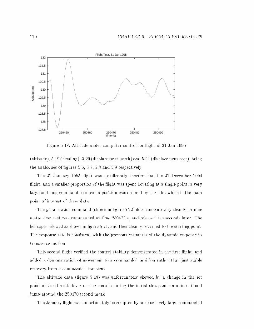
110 CHAPTER 5. FLIGHT-TEST RESULTS
127.5
128
128.5
129
129.5
130
130.5
131
131.5
132
250450 250460 250470 250480 250490
Alti
tude
(m
)
time (s)
Flight Test, 31 Jan 1995
Figure 5.18: Altitude under computer control for ight of 31 Jan 1995
(altitude), 5.19 (heading), 5.20 (displacement north) and 5.21 (displacement east), being
the analogues of �gures 5.6, 5.7, 5.8 and 5.9 respectively.
The 31 January 1995 ight was signi�cantly shorter than the 31 December 1994
ight, and a smaller proportion of the ight was spent hovering at a single point; a very
large and long command to move in position was ordered by the pilot which is the main
point of interest of these data.
The y translation command (shown in �gure 5.22) does come up very cleanly. A nine
metre slew east was commanded at time 250475 s, and released ten seconds later. The
helicopter slewed as shown in �gure 5.21, and then cleanly returned to the starting point.
The response rate is consistent with the previous estimates of the dynamic response in
transverse motion.
This second ight veri�ed the control stability demonstrated in the �rst ight, and
added a demonstration of movement to a commanded position rather than just stable
recovery from a commanded transient.
The altitude data (�gure 5.18) was unfortunately skewed by a change in the set
point of the throttle lever on the console during the initial slew, and an unintentional
jump around the 250470 second mark.
The January ight was unfortunately interrupted by an excessively large commanded
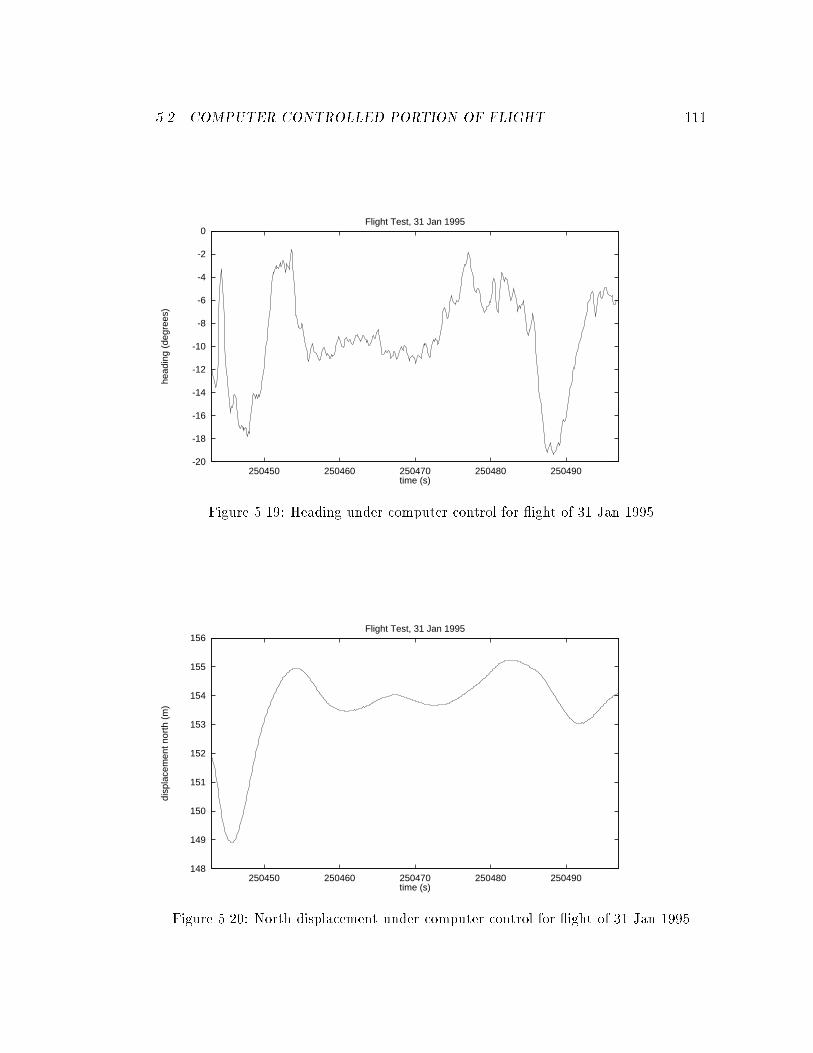
5.2. COMPUTER CONTROLLED PORTION OF FLIGHT 111
-20
-18
-16
-14
-12
-10
-8
-6
-4
-2
0
250450 250460 250470 250480 250490
head
ing
(deg
rees
)
time (s)
Flight Test, 31 Jan 1995
Figure 5.19: Heading under computer control for ight of 31 Jan 1995
148
149
150
151
152
153
154
155
156
250450 250460 250470 250480 250490
disp
lace
men
t nor
th (
m)
time (s)
Flight Test, 31 Jan 1995
Figure 5.20: North displacement under computer control for ight of 31 Jan 1995
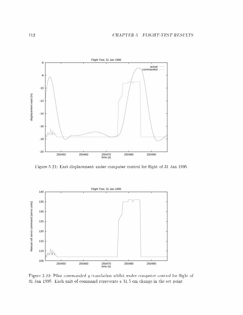
112 CHAPTER 5. FLIGHT-TEST RESULTS
-20
-18
-16
-14
-12
-10
-8
-6
250450 250460 250470 250480 250490
disp
lace
men
t eas
t (m
)
time (s)
Flight Test, 31 Jan 1995
actualcommanded
Figure 5.21: East displacement under computer control for ight of 31 Jan 1995
105
110
115
120
125
130
135
140
250450 250460 250470 250480 250490
Man
ual r
oll s
ervo
com
man
d (s
ervo
uni
ts)
time (s)
Flight Test, 31 Jan 1995
Figure 5.22: Pilot commanded y translation whilst under computer control for ight of31 Jan 1995. Each unit of command represents a 31.5 cm change in the set point.

5.2. COMPUTER CONTROLLED PORTION OF FLIGHT 113
slew in heading at time 250498 s, which caused simultaneously large pitch, roll and yaw
actuations3. This caused loss of GPS satellite visibility and thus the end of the computer
control. Manual control was reenabled, and Steve landed the helicopter safely. Very
high speed slews will have to be pre-limited in future control systems.
3The pitch and roll actuations came from the e�ect of the zero-point biases changing with heading.

Chapter 6
Conclusions and Future Work
This project has accomplished two main aims. The �rst aim (and the original one for
the project) was to demonstrate that GPS { all by itself { is a suitable sensor for total
real-time control of a helicopter. The second aim was to contribute some signi�cant
improvements to GPS algorithms for the situations that arise in automatic control of a
vehicle like a helicopter.
Aim one was demonstrated by the totally autonomous hover control { for the �rst
time { of an (inherently unstable) unmanned helicopter: both position and attitude
were controlled using GPS receivers and antennas as the only sensors.
Aim two was accomplished through the improved integer resolution algorithms for
attitude which allows the use of antennas with poor visibility, and the dynamical method
for dealing with position integers, which allows a vehicle to not have to wait to resolve
position integers.
One of the nicest features of GPS as a sensor is that it is completely electronic. In
particular, as semiconductor technology advances, the sensor electronics will become
smaller and smaller, without the limits that mechanical devices would impose. The
main limit of size will be the GPS antennas themselves. Applying Pournelle's law {
\Silicon is cheap, but iron is expensive." { the overall cost (bulk, mass and raw cost)
will soon become very low. This will make putting this sort of system on small vehicles
exceedingly cost competitive. Indeed, it is plausible that a GPS attitude sensor may
114
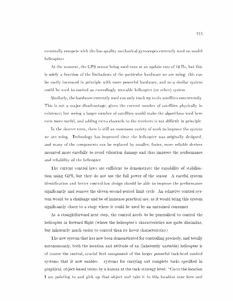
115
eventually compete with the low-quality mechanical gyroscopes currently used on model
helicopters.
At the moment, the GPS sensor being used runs at an update rate of 10 Hz, but this
is solely a function of the limitations of the particular hardware we are using: this can
be vastly increased in principle with more powerful hardware, and so a similar system
could be used to control an exceedingly unstable helicopter (or other) system.
Similarly, the hardware currently used can only track up to six satellites concurrently.
This is not a major disadvantage, given the current number of satellites physically in
existence; but seeing a larger number of satellites would make the algorithms used here
even more useful, and adding extra channels to the receivers is not di�cult in principle.
In the shorter term, there is still an enormous variety of work to improve the system
we are using. Technology has improved since the helicopter was originally designed,
and many of the components can be replaced by smaller, faster, more reliable devices
mounted more carefully to avoid vibration damage and thus improve the performance
and reliability of the helicopter.
The current control laws are su�cient to demonstrate the capability of stabilisa-
tion using GPS, but they do not use the full power of the sensor. A careful system
identi�cation and better control-law design should be able to improve the performance
signi�cantly and remove the eleven-second-period limit cycle. An adaptive control sys-
tem would be a challenge and be of immense practical use, as it would bring this system
signi�cantly closer to a stage where it could be used by an untrained consumer.
As a straightforward next step, the control needs to be generalised to control the
helicopter in forward ight (where the helicopter's characteristics are quite dissimilar,
but inherently much easier to control than its hover characteristics).
The new system that has now been demonstrated for controlling precisely, and totally
autonomously, both the location and attitude of an (inherently unstable) helicopter is
of course the central, crucial �rst component of the larger powerful task-level control
systems that it now enables { systems for carrying out complete tasks speci�ed in
graphical, object-based terms by a human at the task-strategy level: \Go to the location
I am pointing to and pick up that object and take it to this location over here and
116 CHAPTER 6. CONCLUSIONS AND FUTURE WORK
attach it to this fastener.1" It will open up an exciting, broad new era for autonomous
helicopters.
The largest problem with GPS as a sensor is reliability of satellite coverage, especially
when the helicopter is banking signi�cantly. This can be improved in several ways. One
is the addition of new satellites. As the US DoD is unlikely to signi�cantly increase
the number of expensive GPS satellites in the near future, and other organisations are
even less likely, other approaches need to be looked at. The most promising of these
is pseudolites. These are transmitters which appear to a GPS receiver as identical to
a satellite, albeit lacking in orbital parameters and a high-accuracy clock. These have
been used [24] indoors to replace satellites; in principle they could be used to augment
poor satellite visibility.
Another promising approach to increase reliability is to augment the pure-GPS sys-
tem with cheap, light, low quality inertial units, which can be used to maintain control
and an estimate of current position to make up for brief satellite outages.
All in all, using GPS for high-precision, rapid-update automatic control is likely to
become very important in the next decade.
6.1 An aside on Languages
As sensors become more and more abstract, and the role of computers in processing
sensors in automatic control systems becomes more and more signi�cant, the number of
lines of programs involved in the low level, innermost loops of many projects is increasing.
This means that it is worthwhile considering the e�ects of software engineering tools on
such projects.
There is of course a huge software engineering e�ort required in the higher, more
intelligent, levels of control; but the tools for that work are quite similar to tools for
other problems, and there has been extensive work on this serious problem (e.g. [20]).
This section is concerned with the particular needs in compiler code generation relevent
1In the Stanford Aerospace Robotics Laboratory this Task Level Control capability has already beendemonstrated by many systems, such as two dimensional free- ying robots using GPS receivers andpseudolites in [24]
6.1. AN ASIDE ON LANGUAGES 117
to real-time control.
Consider a program whose sole task is to compute GPS positions based on received
phase measurements and line-of-sight vectors. The conventional method of solving this
would be to wait until a matching pair of phase packets have arrived, �nd which satellites
are visible, and set up equation 2.10 and solve it. Then wait for the next packet pair.
The thing to notice here is that there are some calculations that have to be performed
as quickly as possible on order to not introduce any more delay than necessary into the
control loop, and then there is a pause when no useful computation is done.
In multi-user computer systems, this time-based irregularity is not a problem: the
load is shared amongst many users who are unlikely to want all the computation at
once, and overall throughput is biased fairly highly with respect to responsiveness.
Unlike multi-user computers, in embedded computer control systems (and single
user personal computers), it is usually preferable to use otherwise-unallocated time to
precompute as much as possible of the calculation about to be done before all the data
have arrived.
It is perfectly possible, though often messy to perform this with current tools. For
instance, it would be possible to calculate and invert the left-most matrix in equation
2.10 for the expected next time step, for all possible satellite visibilities, or more rea-
sonably, for the most likely ones. However, this makes the program more complex and
harder to understand, debug and maintain, which is deadly in a large project.
It would be very nice to have a language where one would be able to state \If there
is nothing needing to be done, try to execute the following block of code, knowing this
data but not that data." That code would in e�ect then be recompiled, with some
previously variable expressions replaced by constant expressions. Even more convenient
would be if the compiler were capable of doing this automatically, using a cache like
strategy to determine what was most likely to bene�t from precomputation.
A similar sort of problem has been encountered before, in functional languages on
parallel machines. Following is a very brief description of functional languages. An
excellent survey is given in [13]. Functional languages are fairly new and neither well
known nor used commonly, although Ericsson has developed and used extensively an
118 CHAPTER 6. CONCLUSIONS AND FUTURE WORK
impressive functional language called Erlang [4].
A functional language (like APL,Erlang,scheme) di�ers from the more common im-
perative languages in many ways. The most obvious di�erence is that functional lan-
guages have no assignment operator. A variable can only ever contain one value. This is
not as restrictive as it sounds: loops in imperative languages become recursive functions
in functional languages, which can in principle be optimised by a decent compiler into
code as e�cient as imperative languages. Indeed such compilers are just starting to
appear. This removes the existence of global state, and means that the compiler can
recognise that f(a) is always the same, whenever a or f are computed. This property is
called referential transparency. This is not the case in languages such as C. Consider, for
example, the random function, or I/O functions. These have to be handled in functional
languages by passing state into the the function explicitly. This is often inconvenient,
but it has some huge advantages. One advantage is that it is convenient for functions
themselves to be considered as variables, and passed around as parameters and operated
on. Being able to operate on functions is actually an immensely powerful ability. Time
and asynchronous events can also be handled smoothly, e.g. [4, 5].
Another major bene�t of referential transparency is the ability to use lazy evaluation.
Lazy evaluation means that a value does not have to be evaluated until it is needed.
The reason this is useful, is that often expressions are written down, and never used.
What is more, this ine�ciency is often done in a manner that cannot be detected at run
time. For instance, a piece of C code like
double select(int which,double a,double b)
{
if (which) return a;
else return b;
}
...
select(some_var,sin(x),cos(x));
...
6.1. AN ASIDE ON LANGUAGES 119
will cause both sin x and cos x to be evaluated, when only one actually needs to be
evaluated. Of course, it is simple in this example to avoid this problem, but as pro-
grams become more complex it becomes messy to go avoid this sort of situation. Lazy
evaluation also enables some nice programming expressions where the full arguments to
a function may not even be computable in a �nite time.
The process of evaluation in imperative languages like C is called strict evaluation,
and for many functions it is more e�cient than lazy evaluation, as one does not have
to check whether a variable has been evaluated before using it. For this reason, many
functional languages allow a mixture of lazy and strict functions. A function would be
strict in certain arguments if all those arguments are guaranteed to be needed for the
evaluation of the function. This can usually be checked by the compiler.
A compiler then generates code that basically has the job of evaluating expressions.
Some main expression starts the process o�, and then its arguments are evaluated
immediately (if strict) otherwise whenever needed. This process continues recursively,
and thus eventually everything that needs to be is computed.
This type of evaluation is very easy to parallelise to some extent [22]. One has a list
of expressions that need evaluation (based upon strictness de�nitions) and sends them
o� to nearby processors. Due to referential transparency, the order of evaluation does
not matter. However, lazy arguments are a problem here as they may or may not need
to be computed. On a parallel machine, it is eminently possible that there may be some
processors with nothing to do. It is possible to then pass them (at a low priority) the
job of evaluating lazy arguments which may not be needed. Then, if these arguments
are needed, they will be used. If not, then no time has been wasted as those nodes have
nothing else to do. This type of evaluation is called eager or speculative evaluation, and
has been used in microprocessors at the hardware level for a long time for tasks such as
optimising jumps[23].
The reason for mentioning all of this is that this situation is in many ways similar
to the real-time-control situation: one has idle time that is being wasted while new
sensor data are being received. It should be possible to bring some of the compiler
technology over from eager evaluation on parallel machines to eager evaluation of a
120 CHAPTER 6. CONCLUSIONS AND FUTURE WORK
blocked single-processor machine.
Furthermore, one can go signi�cantly further, simplifying expressions when some
sub-expressions are known but not others. For instance, if one had a function evaluating
1 + a2 + b2, and, at some point in execution, the value of b were known, but a was not
known (for whatever reason | in the helicopter scenario it may be that b was some
extrapolated value like a line-of-sight vector and a was some phase measurement that
is expected to come down a serial link `real soon now'). Then, instead of the program
waiting idly for a to arrive, the program could reshape it's internal structure, realising
that 1 + a2 + b2 can be converted into (1 + b2) + a2 which can be partially evaluated
in advance. This could be done either statically, via compiler directives explicitly given
by the programmer \Simplify this function given this expected data," or dynamically
based on a sophisticated caching system learning what data is expected. This of course
could be done in an imperative language like C with some contortions, but it would be
immensely easier to do in a functional language where functions are �rst class objects
and can be manipulated as entities.
The improvements in functional simpli�cation and prediction arising from such re-
search could then feed back in turn to the parallel compiler �eld.
Unfortunately, eager-evaluation technology is still poorly understood other than for
very short look-ahead problems; but I believe that there is an exciting opportunity in
seeing how this technology could be applied to real-time control type problems.
Appendix A
Helicopter manual
This appendix gives some of the details of the hardware used that were not included in
chapter 3 as they were not considered vital to an understanding of the project, but are
useful to people continuing on this project.
A.1 Suppliers
Unusual parts for the electronic boxes (GPS and 486) are given in appendices D and C
respectively. Helicopter equipment can be obtained most readily from Helicopter World1
locally. The portable computer was purchased from PromoX Systems2. The data radios
and antennas came from Metric Systems3. Most miscellaneous GPS equipment came
from Trimble Navigation4.
A.2 Electronic connection
Most of the electrical connections are given in �gures 3.7, 3.8 and 3.10, and are discussed
in chapter 3.
From the exterior, the helicopter appears to be several boxes attached together. In
1521 Sinclair Frontage Rd, Milpitas, CA (408) 942 95252Sunnyvale, CA3San Diego CA (619) 736 00204645 North Mary Avenue Sunnyvale CA 94086
121
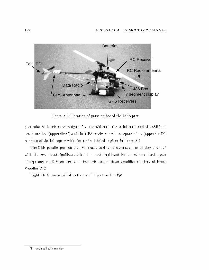
122 APPENDIX A. HELICOPTER MANUAL
Data Radio
GPS Antennae
GPS Receivers
7 segment display486 Box
Batteries
RC Radio antenna
RC ReceiverTail LEDs
Figure A.1: Location of parts on board the helicopter.
particular with reference to �gure 3.7, the 486 card, the serial card, and the 68HC11s
are in one box (appendix C) and the GPS receivers are in a separate box (appendix D).
A photo of the helicopter with electronics labeled is given in �gure A.1.
The 8 bit parallel port on the 486 is used to drive a seven segment display directly5
with the seven least signi�cant bits. The most signi�cant bit is used to control a pair
of high power LEDs on the tail driven with a transistor ampli�er courtesy of Bruce
Woodley A.2.
Eight LEDs are attached to the parallel port on the 486.
5Through a 150 resistor
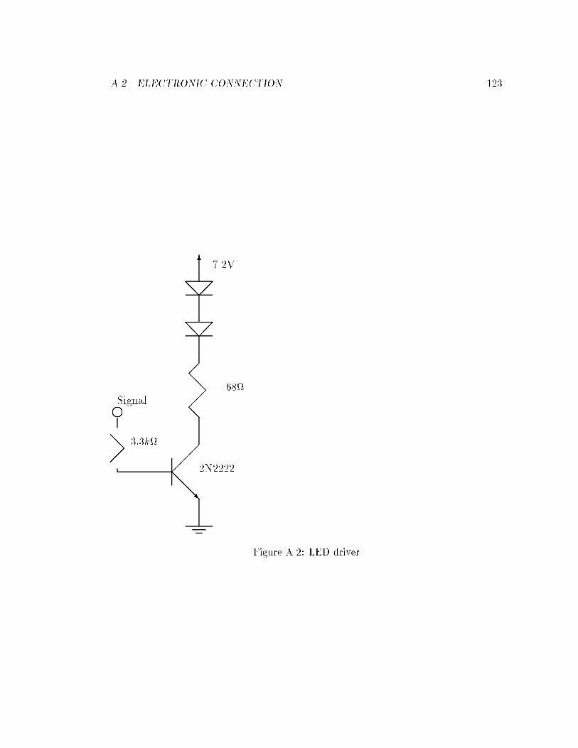
A.2. ELECTRONIC CONNECTION 123
i
��@@
��@@
..........................
@@��...
.......................
��@@��@@
��
�@@@R
6 7.2V
Signal
3:3k
2N2222
68
Figure A.2: LED driver
Appendix B
TSR User's manual
B.1 Introduction
TSR.EXE is a short terminate and stay resident1 program for use on an MS-DOS type
machine. TSR is designed to convert a cheap IBM PC type single board computer,
which has poor support for embedded control and communications, into something that
is not so unpleasant to use.
TSR basically controls serial ports, handling all the low level details so that a higher
level program can just deal with packets being received and transmitted asynchronously.
TSR also has a software-interrupt handle which can be used to command �le transfers,
keyboard emulation, and console emulation. TSR can also store data in XMS memory.
This data can then later be saved to a �le locally, restored from a local disk2, sent down
a serial port, and replayed in real time for debugging purposes.
TSR can make use of the FIFO bu�er in a 16550 UART. TSR is particularly designed
for talking to Trimble TANS GPS receivers, and can understand the packet structure
of these devices.
1MS DOS's form of pseudo multitasking2Typically only useful when used in conjunction with the replaying facility
124

B.2. TECHNICAL DETAILS 125
B.2 Technical Details
This section is designed for someone planning to modify TSR or to write a similar pro-
gram. It is not necessary for the casual user to read this section other than for interest
in some of the design considerations. It is assumed that the reader of this section is
familiar with C++, the Borland C++ compiler, and has some knowledge of the 80x86
and MS DOS architecture.
TSR is written in C++ using the Borland C++ V3.1 compiler, and is compiled in
tiny mode, with the following optimizations: -3 -Ogilt. It uses C++ for data encap-
sulation, rather than for multiple inheritance, so the program should be comprehensible
to someone with a moderate understanding of C++. The comments are not extensive,
though the variable names are generally long and meaningful. The source is optimised
for readability, then speed, then program size.
B.2.1 Segment Registers
Using the tiny memory model rather than a large model reduces code size by almost
a factor of two, and increases execution speed. Unfortunately the tiny model is harder
to use as during interrupts the stack segment will di�er from the data segment. This
means that local variables (on the stack) will not be representable by near pointers, so
one must compile with the option -mt! which speci�es that CS 6= SS. This means that
all the library routines which take an address (such as strlen and open) cannot use local
variables.
Another problem with segment registers occurs when a function in one program (such
as TSR ) is called directly from a di�erent program. Typically, TSR will require that
the DS register point to the start of the TSR data space, whereas the calling program
will have DS set to point to the program's own data space. See section B.6.4 for an
example of the use of such a call. To compensate for this, the callee function must set
the DS register correctly before doing anything else, loading DS from a far variable.
Looking at the assembly language output of the compiler for a sample function call can
help make this problem more comprehensible. When the callee function has returned,
126 APPENDIX B. TSR USER'S MANUAL
the DS register must be restored. Restoring the DS register to an appropriate value for
the caller program is the responsibility of the caller program3
Dealing with the DS and other registers during a software interrupt is handled
automatically by the processor and compiler.
B.2.2 DOS reentrancy
Unfortunately MS DOS is not reentrant. This means that if MS DOS is executing
some function, and then an interrupt occurs, the code in the interrupt handler may not
perform any MS DOS calls. Since TSR must perform various MS DOS functions, such as
writing to the console and accessing disk �les, non-reentrancy is a signi�cant problem.
There are some occasions when an interrupt handler may safely access MS DOS
functions. There are two guaranteed methods of �nding such occasions:
� When a certain memory location (pointed to by indos in this program) is zero.
This is a ag maintained by MS DOS.
� When the DOS idle interrupt is called. This means that MS DOS currently has
control of the computer, but that MS DOS is just sitting in an idle loop waiting
for the user to press a key, and is not using any static variables which would make
it non-reentrant.
When TSR desires to call some MS DOS function, TSR waits until one of the above
opportunities occurs. This may involve keeping a list of things to do at the next op-
portunity. In particular, the clib function printf can not be used during an interrupt,
which makes debugging rather di�cult. TSR includes a set of routines that maintain a
list of things to print out when the timer interrupt is called with (�indos) zero, or theMS DOS idle interrupt is called.
The handles used to access �les are associated with the program currently running.
If TSR is called in an interrupt, the handles associated with the current program will
not necessarily be the handles of TSR . For this reason, one must change the process
3Though the restoration could equally well have been performed as the last action by the calleefunction.
B.2. TECHNICAL DETAILS 127
identi�cation number when one desires to access �les from inside an interrupt in TSR .
This can be done with an uno�cial MS DOS function (encapsulated in SetPID in TSR
). The process identi�cation number must be set back to the original value before the
interrupt returns.
B.2.3 HIMEM.SYS reentrancy
There may be a similar problem with HIMEM.SYS or compatible memory manager.
XMS is used to store data for later extraction and post-processing. It is possible (though
rare) for something to be using XMS which gets interrupted by TSR , which then calls
HIMEM.SYS again. This may cause the system to crash.
There are three main contenders for thing using XMS at the same time as TSR :
� TSR itself { the XMS routines enable interrupts, which means one can not avoid
reentrancy problems by disabling interrupts. This is �xed via a static variable to
check reentrancy.
� The MS DOS system itself { especially if COMMAND.COM is loaded in the high
memory area (HMA). This is dealt with by the rather restrictive assumption that
one can not use XMS whilst DOS is in use. A normal memory bu�er is used while
XMS is not available. When XMS becomes available, the information is coppied
from the temporary bu�er to XMS.
� Some other application program. Caveat emptor. There is no protection imple-
mented against this. Do not use other programs that use XMS with TSR loaded
and receiving and storing data or there is a chance of a crash.
B.2.4 Stack size
There are occasions when the stack usage by TSR during an interrupt is too great to
use the local stack belonging to the application currently being processed. This is
especially true when COMMAND.COM is being reloaded. A solution to this is to use a piece
of preallocated memory for this purpose and load the stack with the address of the base
128 APPENDIX B. TSR USER'S MANUAL
of this preallocated block whenever an interrupt is called (taking care when one has
recursive interrupts). This is implemented in TSR via some assembly code.
B.2.5 Compiler problems
The compiler used is Borland C++ V3.1. It is generally a nice compiler, allowing one
to access registers directly, though the compiler seems to misbehave occasionally when
using this feature by passing a 16 bit register (such as SI) as an argument to a function
taking an 8 bit argument. Do not do this.
There is also a subtle bug associated with using the pascal calling convention with
inline functions containing local variables with destructor methods. Do not do this.
B.2.6 C++ classes
Many C++ classes are used to encapsulate various parts of the program. The program
was originally written in vanilla C, and has been partly converted to C++ to enhance
readability.
no interrupt No interrupt will occur during the scope of a variable of this class. The
constructor checks to see if interrupts are enabled, and if so disables interrupts
and stores the old interrupt enable state. The destructor restores the old state,
allowing safe nesting of instances of this class. This class allows one to isolate a
sensitive piece of code as follows:{
no_interrupt here; // masks interrupts
do_something_sensitive();
if (blah) return;
do_something_else();
}The interrupt enable ag is returned to its previous state on either the termination
of the block of code that is the scope of the variable here, or upon the early exit
at the return statement. This implementation has the advantage of removing the
possibility of forgetting to re-enable interrupts at one of the possibly many exit
B.2. TECHNICAL DETAILS 129
points, of shortening the program source, and of general cleanliness.
change pid Like no interrupt, except this class sets the process identi�cation number
throughout the scope of a variable of this class. This class requires that a global
variable MyPID be initialised before this class is used.
Interrupt Does a partial job of encapsulating an interrupt. Does not contain any
code, but does take care of keeping track of old vectors to make interrupts easier
to deactivate.
Transmit Bu�er Maintains a cyclic character bu�er with interrupt prevention at ap-
propriate locations so that an instance of this class can be used in a reentrant
manner. Used to bu�er data to be transmitted to serial ports as well as to the
console.
Port Basic class to represent a serial port. Handles everything except packet structure.
During an interrupt the appropriate Port class member function needs to be ac-
tivated explicitly and told the address of its service routine, as interrupts do not
provide a parameter giving a pointer to the class.
DataPort A derived class from Port which implements the data packet structure for
the radio and fast ports. (see section B.5.2).
GpsPort A derived class from Port which handles the Trimble packet structure (see
section B.5.1).
Multiple Data Port A class with the same interface as DataPort, but which refer-
ences both the Radio and Fast ports.
connection An inelegant class that handles reliable packet based �le communication
between two computers via a DataPort.
transmit connection A derived class from connection that is speci�cally for the com-
puter that is sending the �le.
130 APPENDIX B. TSR USER'S MANUAL
TSR is designed to be fairly easy to provide support for more serial ports or more
data formats by adding new classes that inherit from Port.
B.2.7 Interrupt Usage
Under MS DOS there is a vectored interrupt scheme, whereby various sources of inter-
rupts cause control to jump to a memory location speci�ed by an interrupt vector. To
add a new interrupt service routine, one replaces the existing location with the address
of the desired new interrupt routine. After processing an interrupt, one may desire to
call (chain on to) the old interrupt processing routine.
There are several interrupts used by TSR :
Serial Ports The serial ports have interrupts that indicate when a byte is received or
ready to be transmitted. Note that if there is nothing to transmit, the ready to
transmit interrupt is masked out. TSR is intelligent enough to allow several serial
ports to share the same interrupt vector, but unfortunately the hardware on IBM
PC type machines rarely supports this as the interrupt lines are not usually driven
by open collector type outputs. This interrupt chains if the function to which one
would chain is part of TSR . This allows sharing of interrupts.
Service Interrupt This is the interrupt that the higher level \user" program calls to
interact with TSR . See section B.6 for a list of the possible commands that can be
sent to TSR . If the value in register AH is not recognised by the service routine,
this interrupt chains.
Clock Interrupt This is called 18.2 times per second. The handler inserts timing
information in the log, and tries to do pending MS DOS operations such as console
output and �le loading or saving if (*indos) is zero. This interrupt handler always
chains.
Character Output This is a software entry point for routines that write to the console.
These are intercepted so that these characters can be sent to an external computer
if desired. This interrupt handler always chains.
B.3. RUNNING THE PROGRAM 131
Dos Safe This interrupt is called whenever MS DOS is in an idle loop and thus one
may safely use MS DOS functions. The interrupt handler does any MS DOS
commands that are needed. This interrupt handler always chains.
B.2.8 Source Files
There is one main C++ �le for TSR called tsr.c, which includes several �les:
emm.h Contains function for dealing with XMS memory.
parallel.h Contains functions for dealing with the parallel port.
serial.h Contains constants for the serial port.
service.h Contains de�nitions to enable a caller program to communicate with TSR .
stack.h Contains functions to switch over to a local stack.
tsr.h Contains the Port class de�nitions.
B.3 Running the program
TSR is a small (about 30k) standard .EXE �le which can be run directly from the
command line. TSR then prints out the status of all the ports and extended memory
which TSR is using and then goes into the background, letting other programs run.
TSR takes many command line options. These all are single strings separated by
spaces. Each string is one command, and consists of either one or two letters, followed
by a number. The letter(s) represent the parameter being varied, and the number
represents the value of the parameter. For on/o� parameters, 0 represents o� and 1
represents on. The one letter commands are global commands; the two letter commands
give values to particular serial ports.
An environment string, GPS TSR ARG, can contain a list of strings separated by spaces
which will also be searched for command line options. There are internal defaults for
settings, which can be superceded by settings in GPS TSR ARG which will be superceded
by command line options.
132 APPENDIX B. TSR USER'S MANUAL
B.3.1 Serial port speci�c ommand line options
These commands all contain two letters followed by a number. The �rst of these letters
speci�es the particular logical port being controlled.
G GPS Port. Typically used to interface to a TANS Quadrex.
A Attitude GPS Port. Typically used to interface to a TANS Vector.
R Radio Port. Used to interface between a ground station and the computer on the
remote vehicle. Typically connected to a radio.
F Fast Port. Very like the radio port, but typically used when the vehicle has landed
and one can connect a high speed serial link directly to the vehicle for faster
down-loads. Typically not used during operations.
The second letter represents the parameter being controlled for that serial port.
s Set speed to the speci�ed baud value. If the parameter is zero, set the serial chip baud
rate divisor to 4. If you do not know what this means, ignore this. The purpose
of this action is to allow a specially modi�ed serial board (see section C.2) to run
at 9600 baud transmit and 38400 baud receive. One needs special hardware for
this.
p Set parity. 0 means no parity, 24 means even parity and 8 means odd parity.
b Set number of bits. Must be 5 to 8.
e Set number of stop bits. Must be 1 or 2.
n Set port number. 0 means deactivate this port. 1-4 means COM1-COM4 respectively
d Debug received packets. Print out the hex packet ID for a packet received on this
channel.
r Debug received data. As soon as a byte is received, print it (in hex).
t Debug sent data. As soon as something is loaded into the serial chip, print the byte
out in hex. Also print out the byte when �rst told to put it in the program bu�er.
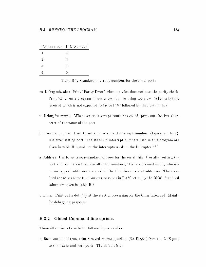
B.3. RUNNING THE PROGRAM 133
Port number IRQ Number
1 4
2 3
3 7
4 5
Table B.1: Standard interrupt numbers for the serial ports.
m Debug mistakes. Print \Parity Error" when a packet does not pass the parity check.
Print `@' when a program misses a byte due to being too slow. When a byte is
received which is not expected, print out `M' followed by that byte in hex.
u Debug interrupts. Whenever an interrupt routine is called, print out the �rst char-
acter of the name of the port.
i Interrupt number. Used to set a non-standard interrupt number. (typically 1 to 7).
Use after setting port. The standard interrupt numbers used in this program are
given in table B.1, and are the interrupts used on the helicopter 486.
a Address. Use to set a non-standard address for the serial chip. Use after setting the
port number. Note that like all other numbers, this is a decimal input, whereas
normally port addresses are speci�ed by their hexadecimal addresses. The stan-
dard addresses come from various locations in RAM set up by the BIOS. Standard
values are given in table B.2
t Timer. Print out a dot (`.') at the start of processing for the timer interrupt. Mainly
for debugging purposes.
B.3.2 Global Command line options
These all consist of one letter followed by a number.
b Base station. If true, echo received relevant packets (5A,ED,84) from the GPS port
to the Radio and Fast ports. The default is on.
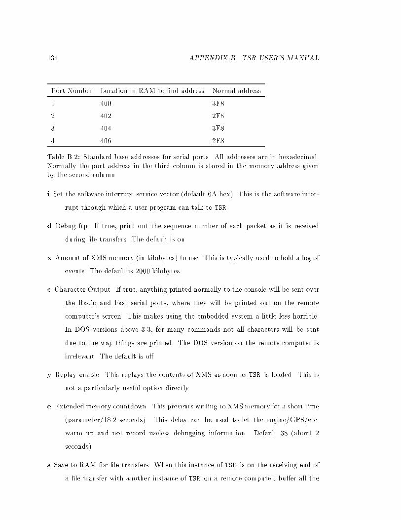
134 APPENDIX B. TSR USER'S MANUAL
Port Number Location in RAM to �nd address Normal address
1 400 3F8
2 402 2F8
3 404 3E8
4 406 2E8
Table B.2: Standard base addresses for serial ports. All addresses are in hexadecimal.Normally the port address in the third column is stored in the memory address givenby the second column.
i Set the software interrupt service vector (default 6A hex). This is the software inter-
rupt through which a user program can talk to TSR .
d Debug ftp. If true, print out the sequence number of each packet as it is received
during �le transfers. The default is on.
x Amount of XMS memory (in kilobytes) to use. This is typically used to hold a log of
events. The default is 2000 kilobytes.
c Character Output. If true, anything printed normally to the console will be sent over
the Radio and Fast serial ports, where they will be printed out on the remote
computer's screen. This makes using the embedded system a little less horrible.
In DOS versions above 3.3, for many commands not all characters will be sent
due to the way things are printed. The DOS version on the remote computer is
irrelevant. The default is o�.
y Replay enable. This replays the contents of XMS as soon as TSR is loaded. This is
not a particularly useful option directly.
e Extended memory countdown. This prevents writing to XMS memory for a short time
(parameter/18.2 seconds). This delay can be used to let the engine/GPS/etc.
warm up and not record useless debugging information. Default 38 (about 2
seconds).
s Save to RAM for �le transfers. When this instance of TSR is on the receiving end of
a �le transfer with another instance of TSR on a remote computer, bu�er all the
B.4. PARALLEL PORT 135
data to XMS before writing to disk. After writing, TSR then veri�es and tries (up
to 5 times) to repair mistakes. This allows packets to not be lost due to slow disk
drives. This is on by default.
B.4 Parallel Port
The parallel port is used as eight logic signals rather than as a strobed device for
data transfer. There are three ways of using the parallel port. The simplest is to set
or reset some bits directly. This is done with the SERVICE SET PARALLEL command,
which enables one to set particular bits (speci�ed by zeros in the mask register BH) to
particular states (speci�ed by register BL). In the helicopter this would be suitable for
controlling a motor used to pull up the disk.
The second method of a�ecting the output is through the COP (computer operating
properly). This is designed to warn of catastrophic failure in either TSR or the program
running above it. TSR is designed so that some program must keep telling TSR that the
computer is still running safely, and whilst this is happening, TSR will oscillate some of
the bits at 9.2 Hz (half the timer interrupt frequency). The particular bits can be set by
the SERVICE SET PARALLEL OSC command. The COP timer is decremented every clock
tick (18.2 times per second) and is reset with the SERVICE SET PARALLEL COP command
which resets the COP timer to the value in the bx register. In the helicopter there is one
bit like this which was once connected to a buzzer which sounded when an oscillating
signal fails. This can be used to indicate catastrophic failure of the GPS or anything
else.
The third method of a�ecting the output is is similar to the COP, and is called by
a similar name, CON (Computer Operating Nicely). This method has a counter in the
same way as the COP whose value is reset to the bx register by the SERVICE SET PARALLEL CON
command. The e�ect of this mode is slightly di�erent to the COP mode, in that this
command sets particular bits high or low depending upon whether CON mode is sat-
is�ed. This action is set by the command SERVICE SET PARALLEL CON ACT. The bits
a�ected are the zero bits in the BH register, and the `proper' behaviour for these bits
136 APPENDIX B. TSR USER'S MANUAL
is set in the BL register. In the helicopter the relevent bit is connected to two 7000
millicandela LEDs, and used to send back non-critical information to someone on the
ground.
B.5 Packet Protocols
B.5.1 GPS packets
These are the standard Trimble protocol. Each packet starts with a DLE (10 hex)
character and ends with the two character sequence DLE ETX (03 hex). The �rst byte
after the �rst DLE is the packet identi�cation number. Intermediate DLE characters
that occur naturally in the data must be escaped by proceeding them with an extra
DLE character.
B.5.2 Radio Packets
Note: This is not important to know unless it is intended to intercept these packets en
route.
The packets sent over the radio link involve a di�erent packet structure. They start
o� with a synchronisation character of 55 hex. Next comes the packet identi�cation
number (one byte) followed by the packet length (one byte, unsigned), followed by the
data. At the end is a parity byte, which is the logical bytewise exclusive or of each of
the preceding bytes in the packet.
This protocol is overlaid with a higher level meta-packet protocol that enables a
device between two PCs running this program to send real time data to one of them,
preempting existing packets without corrupting them. To do this, any of the hex values
ESCCHAR (27 decimal), NULLCHAR (26 decimal) or PWMCHAR (25 decimal) must
be escaped if they occur by preceding them with ESCCHAR. NULLCHARs should
be ignored if encountered in a stream unescaped (this is to support the 68HC11 SPI
communications interface which is not totally asynchronous). The PWMCHAR precedes
a series of 9 bytes containing information on current PWM values, sent to or from a
68HC11.
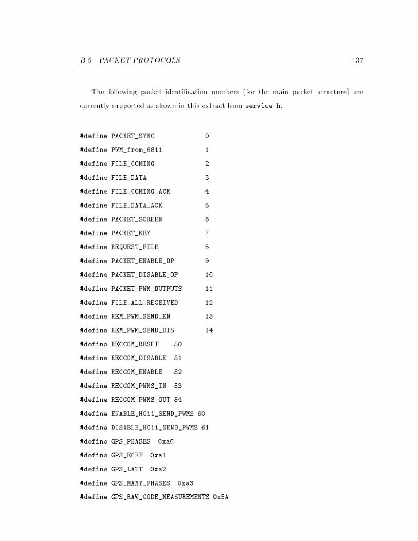
B.5. PACKET PROTOCOLS 137
The following packet identi�cation numbers (for the main packet structure) are
currently supported as shown in this extract from service.h:
#define PACKET_SYNC 0
#define PWM_from_6811 1
#define FILE_COMING 2
#define FILE_DATA 3
#define FILE_COMING_ACK 4
#define FILE_DATA_ACK 5
#define PACKET_SCREEN 6
#define PACKET_KEY 7
#define REQUEST_FILE 8
#define PACKET_ENABLE_OP 9
#define PACKET_DISABLE_OP 10
#define PACKET_PWM_OUTPUTS 11
#define FILE_ALL_RECEIVED 12
#define REM_PWM_SEND_EN 13
#define REM_PWM_SEND_DIS 14
#define RECCOM_RESET 50
#define RECCOM_DISABLE 51
#define RECCOM_ENABLE 52
#define RECCOM_PWMS_IN 53
#define RECCOM_PWMS_OUT 54
#define ENABLE_HC11_SEND_PWMS 60
#define DISABLE_HC11_SEND_PWMS 61
#define GPS_PHASES 0xa0
#define GPS_ECEF 0xa1
#define GPS_LATT 0xa2
#define GPS_MANY_PHASES 0xa3
#define GPS_RAW_CODE_MEASUREMENTS 0x5A

138 APPENDIX B. TSR USER'S MANUAL
B.6 Interface with an external program
An external program can call commands and get data from TSR via the interrupt service
vector (default 6A hex). One calls this routine with some value in the accumulator (AH)
which speci�es the required action. TSR performs that action and returns.
There are various de�nitions in the �le service.hwhich contain symbolic de�nitions
for the commands used below together with some useful type declarations
There is a program called remote.exe which allows a user to perform most of these
commands manually. The program takes a series of arguments, which are all either
commands or arguments to the previous command. In the list below, there are listed
three things: �rstly the symbolic name (as de�ned in service.h). Secondly (in italics)
the commands in remote.exe directly attached with that command, and thirdly a
description of that command.
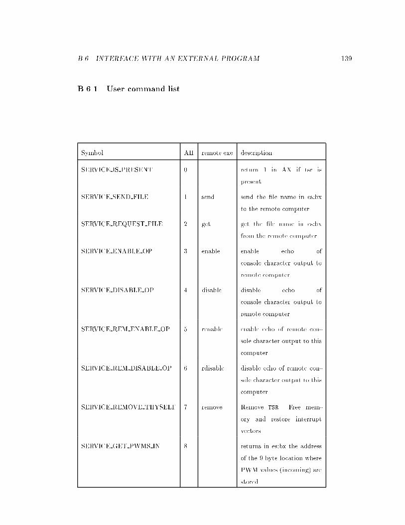
B.6. INTERFACE WITH AN EXTERNAL PROGRAM 139
B.6.1 User command list
Symbol AH remote.exe description
SERVICE IS PRESENT 0 return 1 in AX if tsr is
present
SERVICE SEND FILE 1 send send the �le name in es:bx
to the remote computer
SERVICE REQUEST FILE 2 get get the �le name in es:bx
from the remote computer
SERVICE ENABLE OP 3 enable enable echo of
console character output to
remote computer
SERVICE DISABLE OP 4 disable disable echo of
console character output to
remote computer
SERVICE REM ENABLE OP 5 renable enable echo of remote con-
sole character output to this
computer
SERVICE REM DISABLE OP 6 rdisable disable echo of remote con-
sole character output to this
computer
SERVICE REMOVE THYSELF 7 remove Remove TSR . Free mem-
ory and restore interrupt
vectors.
SERVICE GET PWMS IN 8 returns in es:bx the address
of the 9 byte location where
PWM values (incoming) are
stored
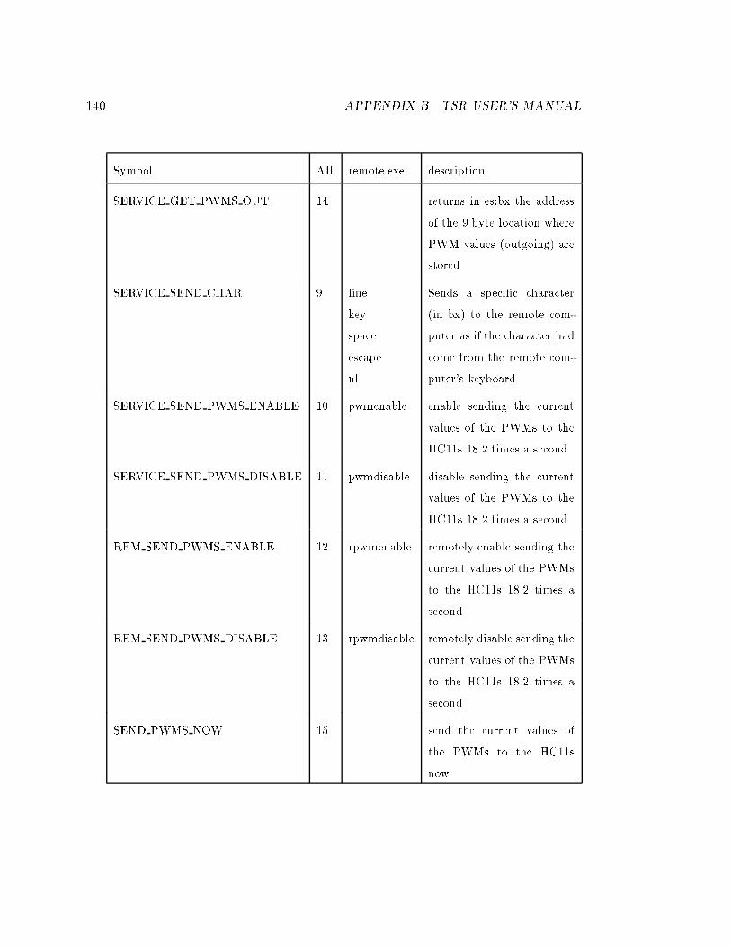
140 APPENDIX B. TSR USER'S MANUAL
Symbol AH remote.exe description
SERVICE GET PWMS OUT 14 returns in es:bx the address
of the 9 byte location where
PWM values (outgoing) are
stored
SERVICE SEND CHAR 9 line
key
space
escape
nl
Sends a speci�c character
(in bx) to the remote com-
puter as if the character had
come from the remote com-
puter's keyboard
SERVICE SEND PWMS ENABLE 10 pwmenable enable sending the current
values of the PWMs to the
HC11s 18.2 times a second
SERVICE SEND PWMS DISABLE 11 pwmdisable disable sending the current
values of the PWMs to the
HC11s 18.2 times a second
REM SEND PWMS ENABLE 12 rpwmenable remotely enable sending the
current values of the PWMs
to the HC11s 18.2 times a
second
REM SEND PWMS DISABLE 13 rpwmdisable remotely disable sending the
current values of the PWMs
to the HC11s 18.2 times a
second
SEND PWMS NOW 15 send the current values of
the PWMs to the HC11s
now.
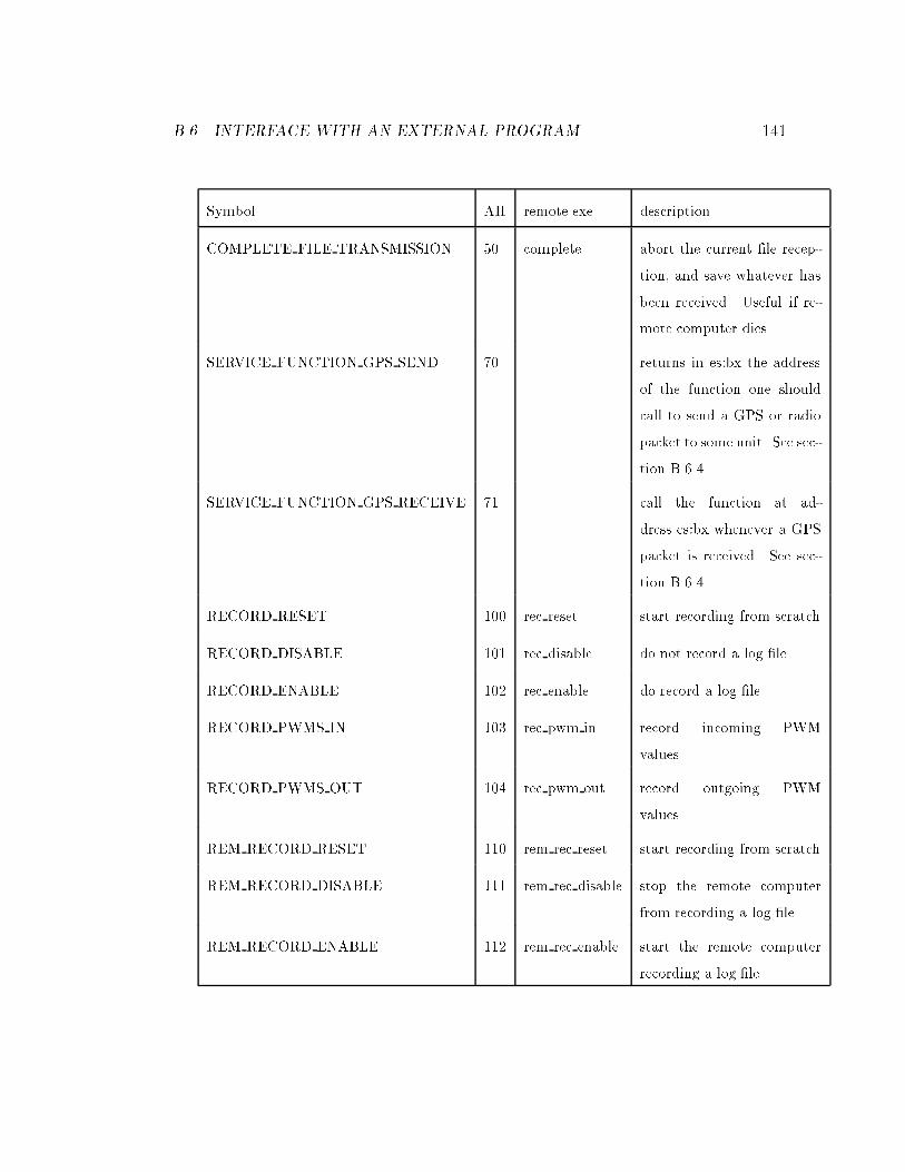
B.6. INTERFACE WITH AN EXTERNAL PROGRAM 141
Symbol AH remote.exe description
COMPLETE FILE TRANSMISSION 50 complete abort the current �le recep-
tion, and save whatever has
been received. Useful if re-
mote computer dies.
SERVICE FUNCTION GPS SEND 70 returns in es:bx the address
of the function one should
call to send a GPS or radio
packet to some unit. See sec-
tion B.6.4.
SERVICE FUNCTION GPS RECEIVE 71 call the function at ad-
dress es:bx whenever a GPS
packet is received. See sec-
tion B.6.4
RECORD RESET 100 rec reset start recording from scratch
RECORD DISABLE 101 rec disable do not record a log �le
RECORD ENABLE 102 rec enable do record a log �le
RECORD PWMS IN 103 rec pwm in record incoming PWM
values
RECORD PWMS OUT 104 rec pwm out record outgoing PWM
values
REM RECORD RESET 110 rem rec reset start recording from scratch
REM RECORD DISABLE 111 rem rec disable stop the remote computer
from recording a log �le
REM RECORD ENABLE 112 rem rec enable start the remote computer
recording a log �le
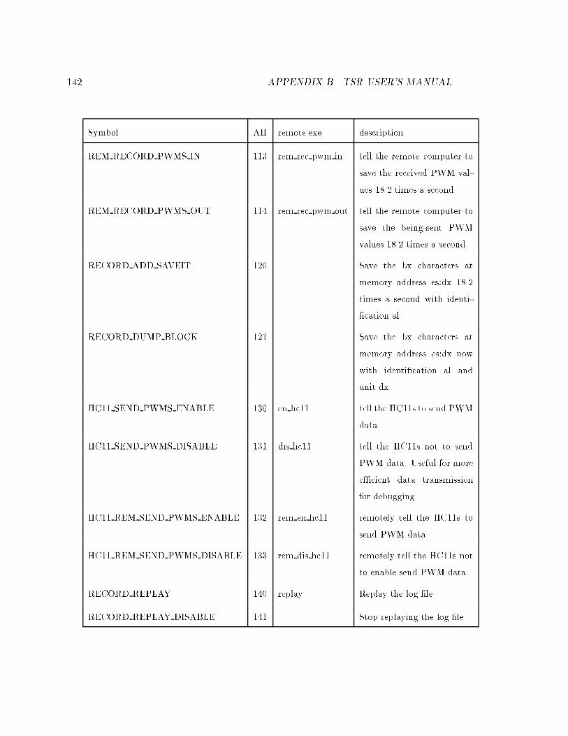
142 APPENDIX B. TSR USER'S MANUAL
Symbol AH remote.exe description
REM RECORD PWMS IN 113 rem rec pwm in tell the remote computer to
save the received PWM val-
ues 18.2 times a second
REM RECORD PWMS OUT 114 rem rec pwm out tell the remote computer to
save the being-sent PWM
values 18.2 times a second
RECORD ADD SAVEIT 120 Save the bx characters at
memory address es:dx 18.2
times a second with identi-
�cation al
RECORD DUMP BLOCK 121 Save the bx characters at
memory address es:dx now
with identi�cation al and
unit dx.
HC11 SEND PWMS ENABLE 130 en hc11 tell the HC11s to send PWM
data.
HC11 SEND PWMS DISABLE 131 dis hc11 tell the HC11s not to send
PWM data. Useful for more
e�cient data transmission
for debugging.
HC11 REM SEND PWMS ENABLE 132 rem en hc11 remotely tell the HC11s to
send PWM data.
HC11 REM SEND PWMS DISABLE 133 rem dis hc11 remotely tell the HC11s not
to enable send PWM data.
RECORD REPLAY 140 replay Replay the log �le
RECORD REPLAY DISABLE 141 Stop replaying the log �le
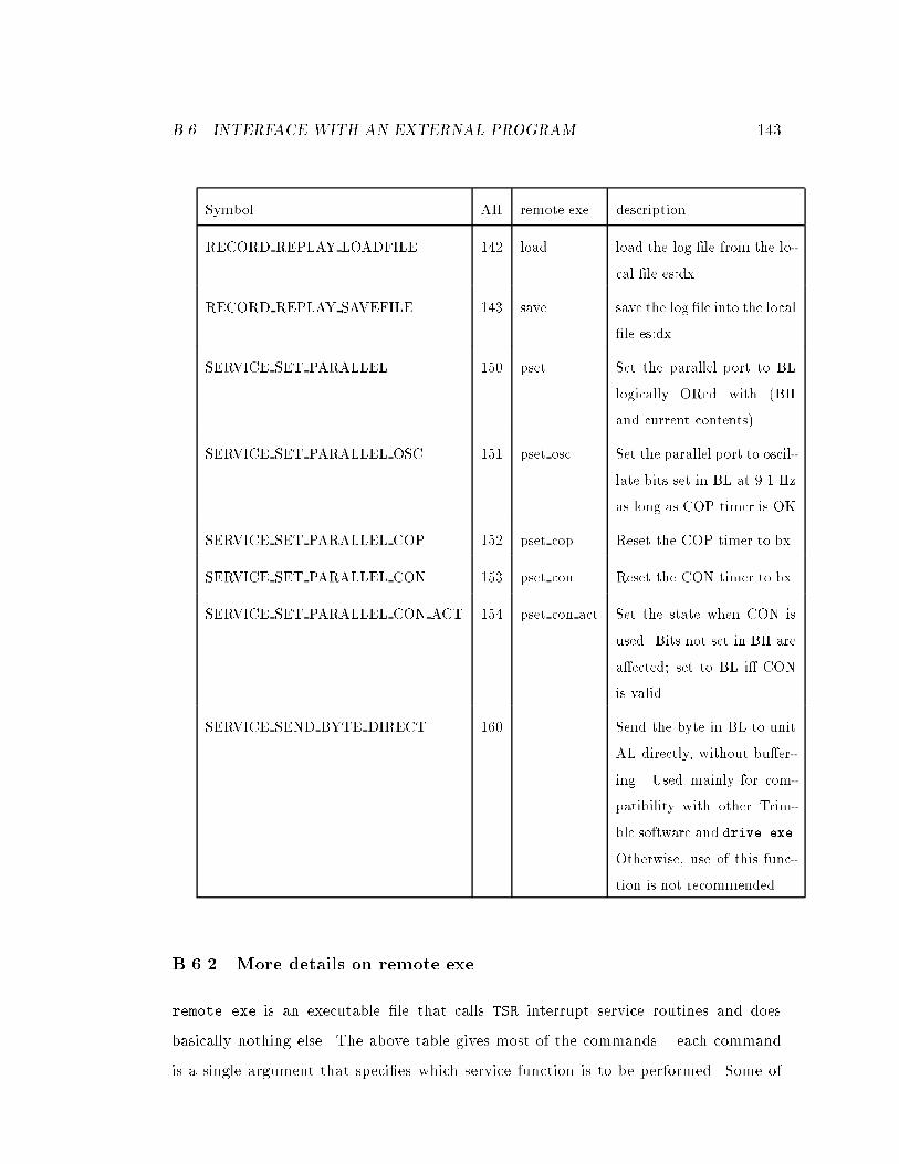
B.6. INTERFACE WITH AN EXTERNAL PROGRAM 143
Symbol AH remote.exe description
RECORD REPLAY LOADFILE 142 load load the log �le from the lo-
cal �le es:dx
RECORD REPLAY SAVEFILE 143 save save the log �le into the local
�le es:dx
SERVICE SET PARALLEL 150 pset Set the parallel port to BL
logically ORed with (BH
and current contents)
SERVICE SET PARALLEL OSC 151 pset osc Set the parallel port to oscil-
late bits set in BL at 9.1 Hz
as long as COP timer is OK
SERVICE SET PARALLEL COP 152 pset cop Reset the COP timer to bx
SERVICE SET PARALLEL CON 153 pset con Reset the CON timer to bx
SERVICE SET PARALLEL CON ACT 154 pset con act Set the state when CON is
used. Bits not set in BH are
a�ected; set to BL i� CON
is valid.
SERVICE SEND BYTE DIRECT 160 Send the byte in BL to unit
AL directly, without bu�er-
ing. Used mainly for com-
patibility with other Trim-
ble software and drive.exe.
Otherwise, use of this func-
tion is not recommended.
B.6.2 More details on remote.exe
remote.exe is an executable �le that calls TSR interrupt service routines and does
basically nothing else. The above table gives most of the commands { each command
is a single argument that speci�es which service function is to be performed. Some of
144 APPENDIX B. TSR USER'S MANUAL
the commands (key, save, load, send and get) take a following parameter. For all other
than key, the next parameter is the string passed to the service routine. For key, each
character in the following parameter is sent one at a time. The special commands space,
nl, and escape send a space, new line and escape key press respectively.
The command line has a slightly di�erent avour. This command takes the rest of
the arguments as key presses and sends them across, interspersed by spaces and followed
by a new line. For instance, the following two lines are equivalent:
remote key copy space key tsr.exe space key newtsr.exe nl
remote line copy tsr.exe newtsr.exe
Some examples would be useful. For instance, to do a directory on the remote
computer:
remote line dir
To send the �le con�g.sys to the remote computer
remote send config.sys
To get the virtual �le EMM.dat (see section B.7)
remote get EMM.dat
B.6.3 Veri�cation: sum.com
There is a program sum.com which computes and prints two checksums for its argument.
This can be used to check that a data transfer went correctly. The �rst checksum is just
the sum of every byte in the program modulo 216; the second checksum has a pseudo-
random weighting for each byte in the program so that this checksum can detect most
swapped bytes.
Typical usage:
A:\sum sum.com
Checksums for sum.com : f829 C763
sum.com has two other uses: if it is invoked with no arguments, the computer will
B.6. INTERFACE WITH AN EXTERNAL PROGRAM 145
beep four times. This can be a handy diagnostic aid occasionally.
If sum.com is invoked with three arguments, it will consider the �rst two arguments
to be �les to read and the third a �le to write. sum.com will produce the third �le from
the logical bitwise `and' operation applied to each byte. This can be used to bypass an
unfortunate bug in writing the EEPROM circuitry on the 486 board; the board in the
helicopter will occasionally writes FF bytes unexpectedly.
B.6.4 GPS packet functions
When a GPS packet is received from either the GPS ports or the data ports from a
remote GPS unit, a certain pointer is checked. If this pointer is non-zero, the pointer is
assumed to be a user function that processes a GPS packet. This function can be set
by using the SERVICE FUNCTION GPS RECEIVE command of TSR (section B.6.1).
A good way to crash the machine is to set this pointer to an invalid address or to a
temporarily valid address, then �nish the program and neglect to set it back to NULL.
The �rst thing this function should do is restore the local DS variable if any global
variables are to be manipulated (which is very very likely).
There is a similar function that enables one to send a packet to a particular GPS unit.
The address of this function can be obtained through the SERVICE FUNCTION GPS SEND
routine. The DS register should be restored after calling this function.
Both functions have the same assumed prototypes:
typedef void far (*send_fn)(int unit,int command,int length,char far *data);
typedef void far (*rec_fn)(int unit,int command,int length,char far *data);
The unit is a number which states to which GPS unit this packet pertains (see section
B.6.5). The command is the packet identi�cation number, the length is the length of
the packet and the data parameter points to the contents of the packet.
One can also use this function to send and receive stu� directly from the radio port.
Any packet with a command not understood by TSR for its internal use that is received
will be passed on to an external program through the same function.
146 APPENDIX B. TSR USER'S MANUAL
B.6.5 GPS Units
There are three types of GPS units, as used in various places such as log �les, packet
reception and packet transmission. One can also send packets to the radio port using
the same functions by using the special unit types UNIT RADIO and UNIT FAST. They
are given symbolic constants in service.h. They are:
� LOCAL GPS [value 0] The local GPS connected to the GPS port
� BASE GPS [value 1] The GPS packets being sent through the Radio port.
� ATT GPS [value 2] The local attitude GPS port.
� UNIT RADIO [value 3] The serial connection to the radio.
� UNIT FAST [value 4] The \fast" serial connection.
B.7 Log �le/XMS
The XMS memory can store a log of the following events:
� GPS packets received from any source
� PWM data
� User information
� Timing information
This data can then be retrieved from the program in three ways:
� Replay in real time (using timing information accurate to 1/18.2 seconds).
� Save directly to a local �le on disk.
� Do a �le transfer of the �le \EMM.dat" (exact capitalisation vital). For this exact
�le name, instead of trying to �nd a disk �le with that name, the program will
send the data in XMS memory exactly as if the XMS memory were a �le. This
is useful for extracting debugging information from an embedded system after a
test ight.

B.8. SKELETON CLIENT PROGRAM 147
B.7.1 Log �le format
The log �le consists of a series of entries. Each entry consists of the following �elds (in
order):
1. (1 byte) Source: Where this data is coming from (such as GPS, or automatic data
capture at each time event. See section B.7.2)
2. (1 byte) Unit: Which unit this refers to. (Such as which GPS unit { section B.6.5).
3. (1 byte) Identi�cation: What the data is. (Such as which packet number for GPS).
4. (1 byte) length: Length of the following data
5. (even number of bytes) data: The data wanted, followed by a �ller byte if length
is odd.
B.7.2 Sources in log �le
The currently de�ned sources in service.h are
SOURCE SAVEITS (value 10) Timing information and regularly saved data.
SOURCE GPS (value 11) GPS packets
SOURCE DUMP (value 12) Data speci�cally instructed to be stored through a direct
call to the service interrupt.
B.8 Skeleton client program
An example skeleton client program is included below
#pragma option -ms -3
/********************************************************\
* *
* Interface.c : Interface to the serial TSR *
148 APPENDIX B. TSR USER'S MANUAL
* For the Helicopter Project *
* *
* (c) Andrew Conway 1993 *
* *
\********************************************************/
#include <dos.h>
#include <string.h>
#include <stdlib.h>
#include <stdio.h>
#include "service.h"
#include "interface.h"
#include <conio.h>
int serial_driver_present()
// returns 1 iff the tsr is loaded, 0 otherwise
{
_AH=SERVICE_IS_PRESENT;
geninterrupt(0x6a);
return _AX==1;
}
void tsr_do_int(int command)
// do a tsr command that has no arguments
{
_AH=command;
geninterrupt(0x6a);
}
void tsr_send_key(char c)
B.8. SKELETON CLIENT PROGRAM 149
// send a keystroke to the remote computer
{
_AH=SERVICE_SEND_CHAR;
_BH=0;
_BL=c;
geninterrupt(0x6a);
}
typedef void far *voidptr;
voidptr tsr_get_ptr(int command)
// call a tsr command that returns a far pointer
{
_AH=command;
geninterrupt(0x6a);
return MK_FP(_ES,_BX);
}
void tsr_send_ptr(int command,void far *v)
// call a tsr command that takes a pointer
{
_ES=FP_SEG(v);
_BX=FP_OFF(v);
_AH=command;
geninterrupt(0x6a);
}
period_get far *pget; // the PWM input vales from the HC11s
period_send far *psend; // the PWM input vales sent to the HC11s
send_fn gps_send; // pointer to function that sends packets
int far restore_ds; // the normal value of the _DS register
150 APPENDIX B. TSR USER'S MANUAL
void far gps_rec(int unit,int command,int length,char far *data)
{
int i;
_DS=restore_ds; // called from elsewhere -- _DS may be wrong
do_something();
}
void tsr_init(void)
{
if (!serial_driver_present()) {
printf("Andrew, you are getting even more absent minded.\n");
printf("LOAD THE SERIAL DRIVER BEFORE RUNNING THIS!\n");
exit(10);
}
pget=(period_get far *)tsr_get_ptr(SERVICE_GET_PWMS_IN);
psend=(period_send far *)tsr_get_ptr(SERVICE_GET_PWMS_OUT);
gps_send=(send_fn)tsr_get_ptr(SERVICE_FUNCTION_GPS_SEND);
tsr_send_ptr(SERVICE_FUNCTION_GPS_RECEIVE,gps_rec);
}
void send_gps(int unit,int command,int len,char *data)
// call this function to send some packet somewhere
{
(*gps_send)(unit,command,len,data);
_DS=restore_ds; // the tsr messes up _DS
}
void main()
{
B.8. SKELETON CLIENT PROGRAM 151
restore_ds=_DS;
tsr_init();
for (;;) do_something();
tsr_send_ptr(SERVICE_FUNCTION_GPS_RECEIVE,0L);
// disable gps_rec
}
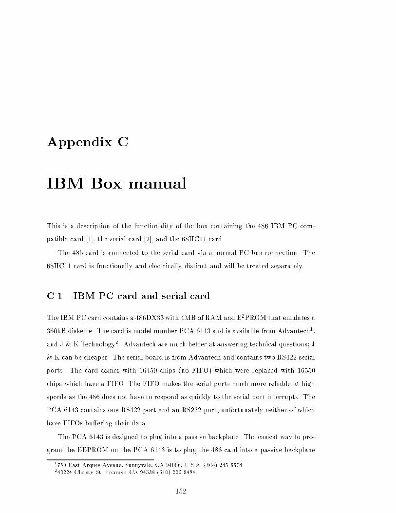
Appendix C
IBM Box manual
This is a description of the functionality of the box containing the 486 IBM PC com-
patible card [1], the serial card [2], and the 68HC11 card.
The 486 card is connected to the serial card via a normal PC bus connection. The
68HC11 card is functionally and electrically distinct and will be treated separately.
C.1 IBM PC card and serial card
The IBM PC card contains a 486DX33 with 4MB of RAM and E2PROM that emulates a
360kB diskette. The card is model number PCA 6143 and is available from Advantech1,
and J & K Technology2. Advantech are much better at answering technical questions; J
& K can be cheaper. The serial board is from Advantech and contains two RS422 serial
ports. The card comes with 16450 chips (no FIFO) which were replaced with 16550
chips which have a FIFO. The FIFO makes the serial ports much more reliable at high
speeds as the 486 does not have to respond as quickly to the serial port interrupts. The
PCA 6143 contains one RS422 port and an RS232 port, unfortunately neither of which
have FIFOs bu�ering their data.
The PCA 6143 is designed to plug into a passive backplane. The easiest way to pro-
gram the EEPROM on the PCA 6143 is to plug the 486 card into a passive backplane
1750 East Arques Avenue, Sunnyvale, CA 94086, U.S.A. (408) 245 6678243224 Christy St. Fremont CA 94538 (510) 226 9484
152
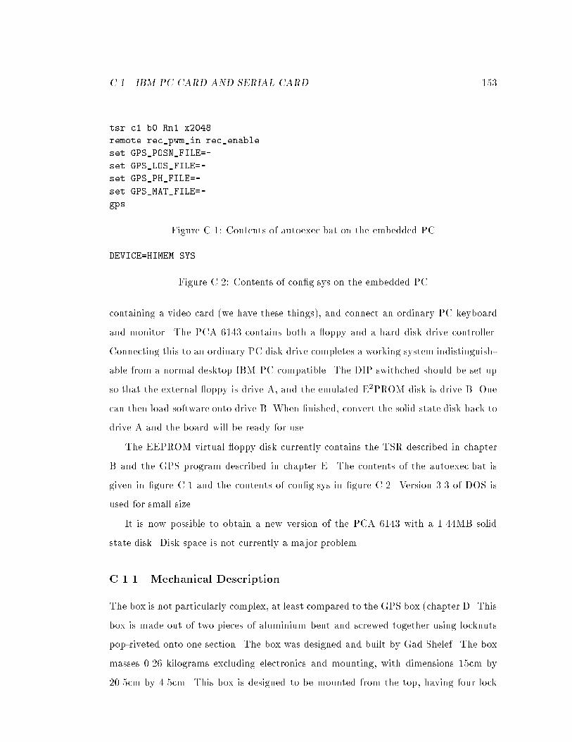
C.1. IBM PC CARD AND SERIAL CARD 153
tsr c1 b0 Rn1 x2048
remote rec_pwm_in rec_enable
set GPS_POSN_FILE=-
set GPS_LOS_FILE=-
set GPS_PH_FILE=-
set GPS_MAT_FILE=-
gps
Figure C.1: Contents of autoexec.bat on the embedded PC
DEVICE=HIMEM.SYS
Figure C.2: Contents of con�g.sys on the embedded PC
containing a video card (we have these things), and connect an ordinary PC keyboard
and monitor. The PCA 6143 contains both a oppy and a hard disk drive controller.
Connecting this to an ordinary PC disk drive completes a working system indistinguish-
able from a normal desktop IBM PC compatible. The DIP swithched should be set up
so that the external oppy is drive A, and the emulated E2PROM disk is drive B. One
can then load software onto drive B. When �nished, convert the solid state disk back to
drive A and the board will be ready for use.
The EEPROM virtual oppy disk currently contains the TSR described in chapter
B and the GPS program described in chapter E. The contents of the autoexec.bat is
given in �gure C.1 and the contents of con�g.sys in �gure C.2. Version 3.3 of DOS is
used for small size.
It is now possible to obtain a new version of the PCA 6143 with a 1.44MB solid
state disk. Disk space is not currently a major problem.
C.1.1 Mechanical Description
The box is not particularly complex, at least compared to the GPS box (chapter D. This
box is made out of two pieces of aluminium bent and screwed together using locknuts
pop-riveted onto one section. The box was designed and built by Gad Shelef. The box
masses 0.26 kilograms excluding electronics and mounting, with dimensions 15cm by
20.5cm by 4.5cm. This box is designed to be mounted from the top, having four lock
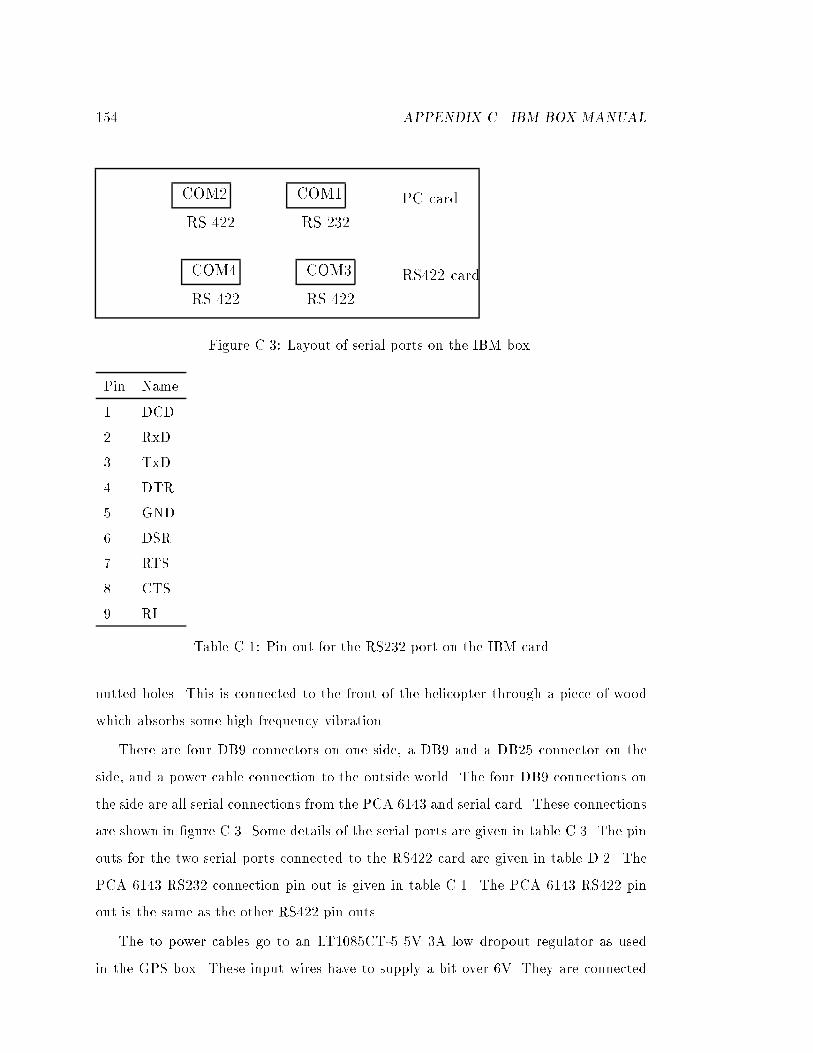
154 APPENDIX C. IBM BOX MANUAL
RS 422 RS 232
RS 422 RS 422
COM3COM4
COM2 COM1 PC card
RS422 card
Figure C.3: Layout of serial ports on the IBM box.
Pin Name
1 DCD
2 RxD
3 TxD
4 DTR
5 GND
6 DSR
7 RTS
8 CTS
9 RI
Table C.1: Pin out for the RS232 port on the IBM card
nutted holes. This is connected to the front of the helicopter through a piece of wood
which absorbs some high frequency vibration.
There are four DB9 connectors on one side, a DB9 and a DB25 connector on the
side, and a power cable connection to the outside world. The four DB9 connections on
the side are all serial connections from the PCA 6143 and serial card. These connections
are shown in �gure C.3. Some details of the serial ports are given in table C.3. The pin
outs for the two serial ports connected to the RS422 card are given in table D.2. The
PCA 6143 RS232 connection pin out is given in table C.1. The PCA 6143 RS422 pin
out is the same as the other RS422 pin outs.
The to power cables go to an LT1085CT-5 5V 3A low dropout regulator as used
in the GPS box. These input wires have to supply a bit over 6V. They are connected
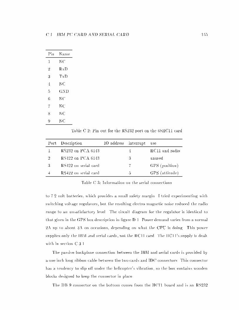
C.1. IBM PC CARD AND SERIAL CARD 155
Pin Name
1 NC
2 RxD
3 TxD
4 NC
5 GND
6 NC
7 NC
8 NC
9 NC
Table C.2: Pin out for the RS232 port on the 68HC11 card
Port Description IO address interrupt use
1 RS232 on PCA 6143 4 HC11 and radio
2 RS422 on PCA 6143 3 unused
3 RS422 on serial card 7 GPS (position)
4 RS422 on serial card 5 GPS (attitude)
Table C.3: Information on the serial connections
to 7.2 volt batteries, which provides a small safety margin. I tried experimenting with
switching voltage regulators, but the resulting electro magnetic noise reduced the radio
range to an unsatisfactory level. The circuit diagram for the regulator is identical to
that given in the GPS box description in �gure D.1. Power demand varies from a normal
2A up to about 3A on occasions, depending on what the CPU is doing. This power
supplies only the IBM and serial cards, not the HC11 card. The HC11's supply is dealt
with in section C.3.1.
The passive backplane connection between the IBM and serial cards is provided by
a one inch long ribbon cable between the two cards and IDC connectors. This connector
has a tendency to slip o� under the helicopter's vibration, so the box contains wooden
blocks designed to keep the connector in place.
The DB 9 connector on the bottom comes from the HC11 board and is an RS232
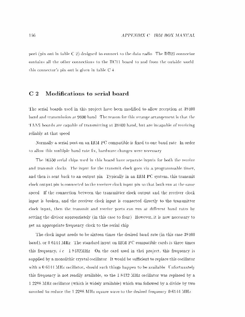
156 APPENDIX C. IBM BOX MANUAL
port (pin out in table C.2) designed to connect to the data radio. The DB25 connector
contains all the other connections to the HC11 board to and from the outside world.
this connector's pin out is given in table C.4.
C.2 Modi�cations to serial board
The serial boards used in this project have been modi�ed to allow reception at 38400
baud and transmission at 9600 baud. The reason for this strange arrangement is that the
TANS boards are capable of transmitting at 38400 baud, but are incapable of receiving
reliably at that speed.
Normally a serial post on an IBM PC compatible is �xed to one baud rate. In order
to allow this multiple baud rate �x, hardware changes were necessary.
The 16550 serial chips used in this board have separate inputs for both the receive
and transmit clocks. The input for the transmit clock goes via a programmable timer,
and then is sent back to an output pin. Typically in an IBM PC system, this transmit
clock output pin is connected to the receiver clock input pin so that both run at the same
speed. If the connection between the transmitter clock output and the receiver clock
input is broken, and the receiver clock input is connected directly to the transmitter
clock input, then the transmit and receive ports can run at di�erent baud rates by
setting the divisor appropriately (in this case to four). However, it is now necessary to
get an appropriate frequency clock to the serial chip.
The clock input needs to be sixteen times the desired baud rate (in this case 38400
baud), or 0.6144 MHz. The standard input on IBM PC compatible cards is three times
this frequency, i.e. 1.8432MHz. On the card used in thei project, this frequency is
supplied by a monolithic crystal oscillator. It would be su�cient to replace this oscillator
with a 0.6144 MHz oscillator, should such things happen to be available. Unfortunately
this frequency is not readily available, so the 1.8432 MHz oscillator was replaced by a
1.2288 MHz oscillator (which is widely available) which was followed by a divide by two
counted to reduce the 1.2288 MHz square wave to the desired frequency 0.6144 MHz.
C.3. TIMER (68HC11) BOARD 157
A spare 7474 was found on the serial card3 and was used as the divide by two counter.
Thus this modi�cation did not require any additional electronics mounted on the board,
only a replacement of the oscillator, a few cut PCB traces and some new wires.
C.3 Timer (68HC11) board
This board contains two Motorola MC68HC811E2microcontrollers. Each has four timer
channels which are used to receive the pulse width modulated signals from the normal
remote control radio. Depending upon the state of a certain input (input 1) the 68HC11s
can either pass the radio signals directly through or put out their own control signals.
This provides the ability for the operator to switch the helicopter over to manual control
at any stage, assuming that this circuit is reliable.
The circuit has a secondary feature of passing through RS232 signals from an external
radio to the main computer. Data ow can be visualised as starting from the data
modem radio at 9600 baud. This passes to the slave 68HC11 through its SCI serial
port. The slave 68CH11 then sends this data (plus the values of its PWM inputs)
to the master 68HC11 over the two devices' SPI serial port. The SPI port is rather
nonstandard, and synchronisation is very time critical. The SPI runs at about 16000
baud. The master 68HC11 adds in its own PWM data and sends all the PWM values
on to the main computer (the 486 card) via its SCI connection at RS232 voltage levels.
No RS232 handshaking is used: it is assumed that the devices the HC11s are connected
to can always accept data. This is for several reasons:
� It would require extra complexity
� The HC11s don't have enough RAM to bu�er the data for long
� Even if the 68HC11s did have su�cient RAM, delaying data for that length of
time would almost certainly be wrong for other reasons due to the need for up to
date information for control.
3This 7474 was normally used to enable or disable the output drivers when the board was acting asan RS485 port. This facility was not needed.
158 APPENDIX C. IBM BOX MANUAL
� Even if there were some reason to bank up old data, the main computer is always
ready to accept data, and the radio is never ready to accept data.
A corresponding ow of data exists in the opposite direction due to the main com-
puter sending the computed servo command values to the master HC11 which extracts
the four PWM values handled by the master HC11 and passes the other four PWM
values on to the slave HC11. The slave HC11 will then pass any data packets sent on to
the radio, which will promptly ignore these data as the radio is half duplex and set up
to only receive on the helicopter as it is much more important for the helicopter to get
information from the ground than vice versa. The IBM cannot command the HC11s
to change between computer and manual control | this can only be commanded by a
switch on the remote control console.
C.3.1 Power for HC11 board
Power for this circuit comes independently of the power for the 486 computer. The
power source comes directly from a 4.8V battery pack with a lifetime longer than the
486 batteries' lifetime4 . This is because the HC11 board is more important for helicopter
survival.
There are two 4.8V battery packs used: one to power the servos and one to power
the radio and HC11 board. This is done to prevent the very large power glitches in the
servos from a�ecting the (relatively) delicate HC11s.
C.3.2 Board construction
This is a custom board designed by me and built by Godwin Zhang. The circuit diagram
is given in �gure C.4 and the circuit diagram for the connector is given in �gure C.5.
The circuit contains two 68HC811E2microcontrollers. These contain on chip E2PROM
to store the program, a standard serial port (SCI), a nonstandard serial port (SPI) and
four timer channels each.
The reset signal is generated by a low voltage detector (34064), the clock signal by
4For the amounts of current typically drawn from each battery
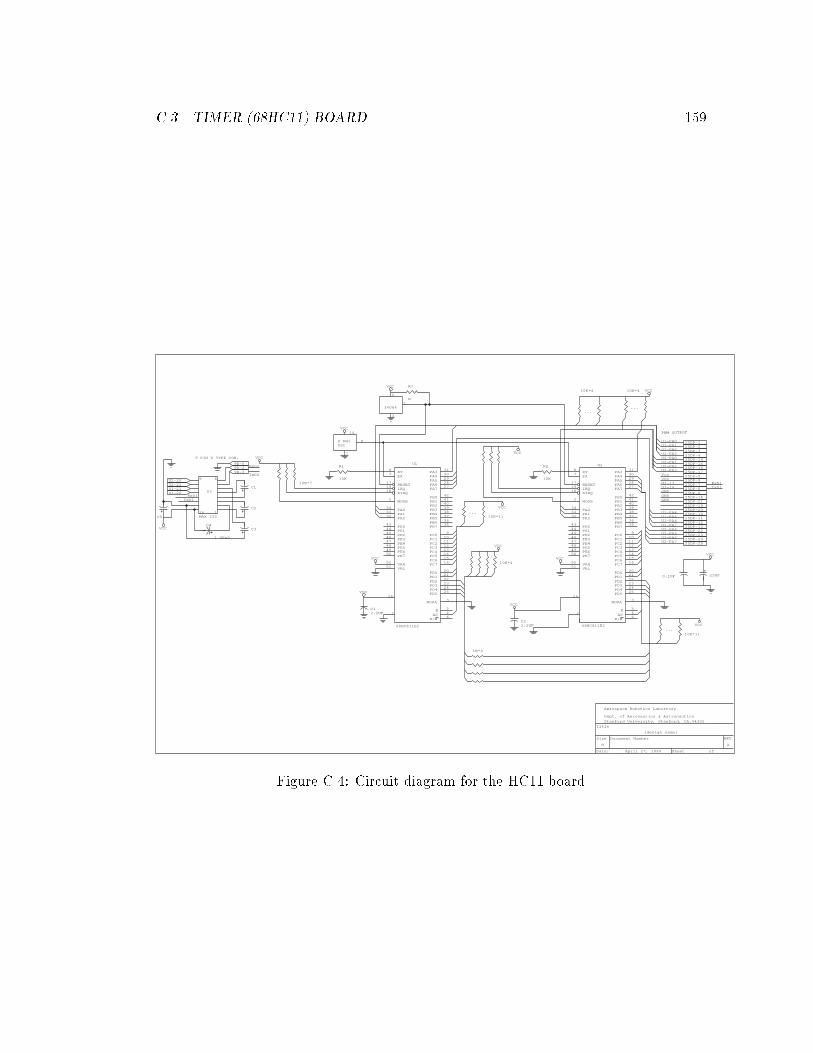
C.3. TIMER (68HC11) BOARD 159
Date: April 27, 1994 Sheet of
Size Document Number REV
B A
Title
[design name]
Stanford University, Stanford, CA.94305
Dept. of Aeronautics & Astronautics
Aerospace Robotics Labortory
10K*4 VCC10K*4VCC R?
R2
VCC
8 MHz 8
14
OSC
1
3
34064
VCC
......
PWM OUTPUT
U1-PA0U1-PA1U1-PA2
25DP-125DP-225DP-3
25DP-1425DP-1525DP-1625DP-17
25DP-1825DP-21
U1-PA3U2-PA0U2-PA1U2-PA2U2-PA3
25DP-4
VccvCCU3-13U3-14GNDGNDGND
25DP-525DP-925DP-725DP-825DP-6
RxD1TxD1
XT 8
EX 7
RESET 17
IRQ 19
XIRQ 18
MODB 2
PA0 34
PA1 33
PA2 32
PE0 43
PE1 44
PE2 45
PE3 46
PE4 47
PE5 48
PE6 49
PE7 50
VRH 52
VRL 51
PA331
PA430
PA529
PA628
PA727
PB042
PB141
PB240
PB339
PB438
PB537
PB636
PB735
PC0 9
PC110
PC211
PC312
PC413
PC514
PC615
PC716
PD020
PD121
PD222
PD323
PD424
PD525
MODA 3
E 5
AS 4
R/W 6
U2
68HC811E2
R2
10K
VCC
XT 8
EX 7
RESET 17
IRQ 19
XIRQ 18
MODB 2
PA0 34
PA1 33
PA2 32
PE0 43
PE1 44
PE2 45
PE3 46
PE4 47
PE5 48
PE6 49
PE7 50
VRH 52
VRL 51
PA331
PA430
PA529
PA628
PA727
PB042
PB141
PB240
PB339
PB438
PB537
PB636
PB735
PC0 9
PC110
PC211
PC312
PC413
PC514
PC615
PC716
PD020
PD121
PD222
PD323
PD424
PD525
MODA 3
E 5
AS 4
R/W 6
U1
68HC811E2
7
R1
10K
VCC
9D-39D-29D-5
10K*7C1
RxD2
TxD289
U1-21U2-21
U1-20
U2-20
9 PIN D TYPE CON.
U3RxD1
TxD1
116MAX 232
VCC
1 UFx5
C5
C4C3
C2...
VCC
10K*1125DP-1025DP-1125DP-1225DP-1325DP-2225DP-2325DP-2425DP-25U2-PA7
U1-PA4U1-PA5U1-PA6U1-PA7U2-PA4U2-PA5U2-PA6
25DP-1925DP-20
0.1UF 25UF
VCCVCC
26
10K*4VCC
26VCC
C12.2UF 1
VCC
C22.2UF
1
...
VCC
10K*11
1K*4
Figure C.4: Circuit diagram for the HC11 board

160 APPENDIX C. IBM BOX MANUAL
Date: May 26, 1994 Sheet of
Size Document Number REV
B A
Title
Helicopter Micro-controller Power/Data Cable
Stanford University, Stanford, CA.94305
Dept. of Aeronautics & Astronautics
Aerospace Robotics Labortory
VccVCC
3-PIN CONNECTOR, PLUG
VCCU1PA1
GND
U1PA0GND
VCCU1PA2
GND
VCC
25D CONNECTOR
25DS-125DS-225DS-325DS-425DS-1425DS-1525DS-16
25DS-525DS-18
F-M
Vcc
GND
U1PA3GND
VCC
GND
VCCU2PA1
GND
VCC
U2PA0
U2PA2GND
VCCU2PA3
GND
9D-5
VCCGND
3-PIN CONNECTOR, SOCKET
25DS-6
25DS-1725DS-925DS-22
Vcc
GND
GND
25DS-725DS-8
25DS-425DS-325DS-225DS-125DS-1425DS-1525DS-1625DS-17
RxTx9D-2
9D-3
VCCGND
AUX3
9D CONNECTORM-F
GEAR
AUX1
AUX2VCCGND
VCCGND
VCCGND
1A1 2
1A2 4
1A3 6
1A4 8
2A1 11
2A2 13
2A3 15
2A4 17
1G 1
2G 19
1Y118
1Y216
1Y314
1Y412
2Y1 9
2Y2 7
2Y3 5
2Y4 3
U?
74HC244
Vcc
GND
ELEV
RUDDVCCGND
VCCGND
THRO
AILEVCCGND
VCCGND
3-PIN CONNECTOR, SOCKET
Figure C.5: Circuit diagram for the connector to the HC11 board, radios, Servos and486.
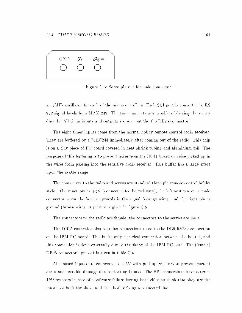
C.3. TIMER (68HC11) BOARD 161
� ��
� ��
� ��
�� @@GND 5V Signal
Figure C.6: Servo pin out for male connector
an 8MHz oscillator for each of the microcontrollers. Each SCI port is converted to RS
232 signal levels by a MAX 232. The timer outputs are capable of driving the servos
directly. All timer inputs and outputs are sent out the the DB25 connector.
The eight timer inputs come from the normal hobby remote control radio receiver.
They are bu�ered by a 74HC244 immediately after coming out of the radio. This chip
is on a tiny piece of PC board covered in heat shrink tubing and aluminium foil. The
purpose of this bu�ering is to prevent noise from the HC11 board or noise picked up in
the wires from passing into the sensitive radio receiver. This bu�er has a large e�ect
upon the usable range.
The connectors to the radio and servos are standard three pin remote control hobby
style. The inner pin is +5V (connected to the red wire), the leftmost pin on a male
connector when the key is upwards is the signal (orange wire), and the right pin is
ground (brown wire). A picture is given in �gure C.6
The connectors to the radio are female; the connectors to the servos are male.
The DB25 connector also contains connections to go to the DB9 RS232 connection
on the IBM PC board. This is the only electrical connection between the boards, and
this connection is done externally due to the shape of the IBM PC card. The (female)
DB25 connector's pin out is given in table C.4.
All unused inputs are connected to +5V with pull up resistors to prevent current
drain and possible damage due to oating inputs. The SPI connections have a series
1k resistors in case of a software failure forcing both chips to think that they are the
master or both the slave, and thus both driving a connected line.
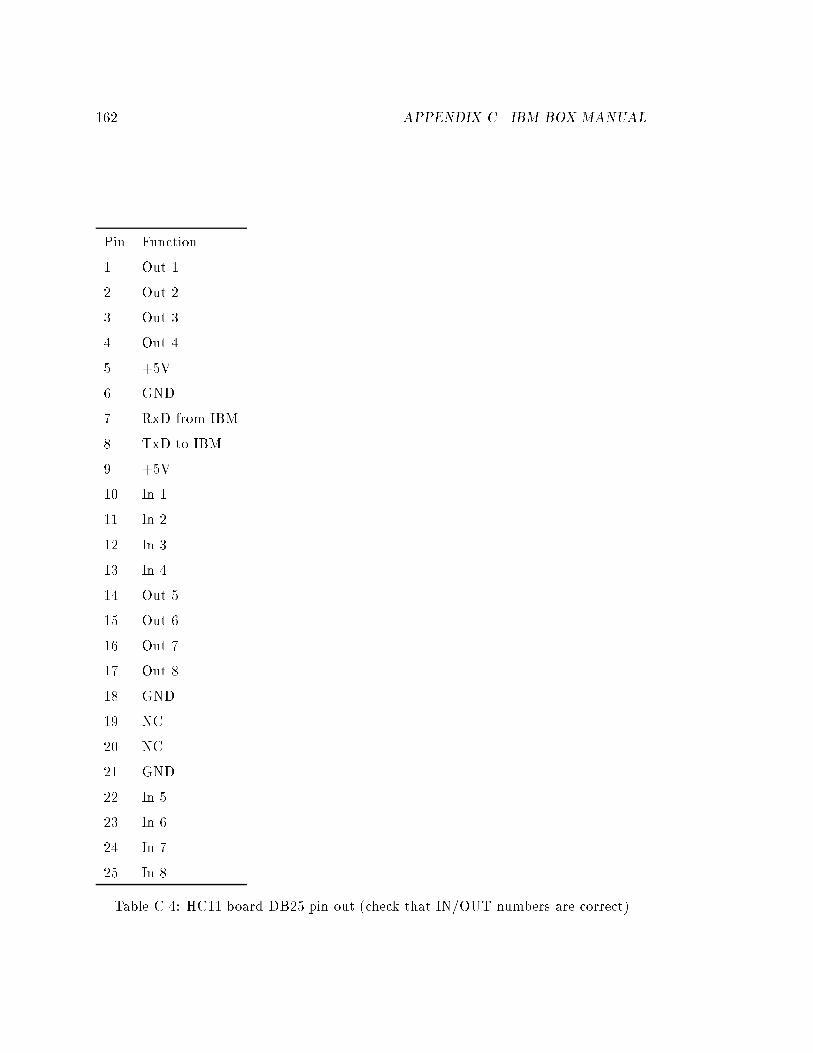
162 APPENDIX C. IBM BOX MANUAL
Pin Function
1 Out 1
2 Out 2
3 Out 3
4 Out 4
5 +5V
6 GND
7 RxD from IBM
8 TxD to IBM
9 +5V
10 In 1
11 In 2
12 In 3
13 In 4
14 Out 5
15 Out 6
16 Out 7
17 Out 8
18 GND
19 NC
20 NC
21 GND
22 In 5
23 In 6
24 In 7
25 In 8
Table C.4: HC11 board DB25 pin out (check that IN/OUT numbers are correct)
C.4. PROGRAMS RUNNING ON HC11 163
C.4 Programs Running on HC11
There are two HC11s; each runs a slightly separate program. There are several reasons
for the di�erences:
� The Motorola SPI interface is inherently non-symmetric, requiring one device to
be the master and one device to be the slave
� Only one device (the master) talks to the 486
� Only one device reads the PWM signal that means pass through or block.
There are eight logical PWM inputs and outputs, as seen by the external IBM.
These are numbered 1 to 8. The �rst four are the master channels 1 to 4, the second
four are the slave channels 1-4. Channel 1 controls whether the PWM values will be
passed straight through or the IBM supplied values will be used. Internally the timers
are quantized to 16 bit values (0:5�S), and in pass though mode the 16 bit values are
used. When talking with the IBMs, only an 8 bit range is used to preserve bandwidth.
These 8 bit values are given by the formula
min(0;max(255;16 bit value � PWM MINIMUM
4)) (C:1)
A description of how the 68HC11 programs work is given here in case they need to
be modi�ed. Such modi�cation is to be avoided as this program controls the manual
override and is this absolutely critical to the safety of the helicopter. The HC11s and
programs have been weell tested in their current con�guration. The following descrip-
tion is given with signi�cant detail as interrupt driven assembly language is di�cult to
understand.
Both programs start o� with a whole lot of de�nes. These are symbolic names for
the special purpose registers on the 68HC11 family. They were taken from a program
HEXMON.ASM by Fred. G. Martin. No HC11 program should leave home without them.
Next come a list of variables. These are global variables with �xed location in RAM.
A description of these registers follows, with a description of how some of the algorithms
work:
164 APPENDIX C. IBM BOX MANUAL
timer over ow This is a 2 byte value which can (but isn't) be used to times tamp
events with a full 32 bit time, using these 2 bytes as the upper word and the
internal HC11 16 bit timer as the lower 16 bits. This variable is incremented by
the timer over ow interrupt.
may send spi On the master, a timer value that says when it is next time to send a
value over the SPI. This value is polled in the main loop rather than interrupted.
ag send spi On the master, a ag that is zero i� the master is currently sending a
message on the SPI.
pwmNin For N between 1 and 4, gives the 16 bit value of the PWM signal on input
N for this chip. The pulse width is measured in units of 0:5�S. This value is
maintained by interrupts.
pwmNout For N between 1 and 4, gives the 16 bit value of the PWM signal to be
produced on output N for this chip. The pulse width is measured in units of 0:5�S.
This value is maintained by interrupts.
SendPWMs A ag byte sent from the IBM regularly (or whenever the IBM decides
to do so). If this byte is non-zero, the IBM wishes to have regular updates of the
PWM signals.
IBMpwmN For N between 1 and 8. These are the 8 logical PWM commands from
the IBM. Connections 1-4 are not needed by the slave so they are not stored.
toIBMN for N between 1 and 8. These are the 8 logical PWM input values to be sent
to the IBMs. The master knows all of these since the master HC11 is sent the
slave's values; the slave only knows its own plus the value of channel 1, which is
needed for the mode (pass through/IBM controlled) selection.
ICN wenthigh for N between 0 and 4. The timer value when the PWM signal for
input capture (IC) number N went high. These are maintained by interrupts. The
pwnNin values are maintained by interrupt routines that are called whenever one
of the PWM inputs changes state. If the PWM went high, the latched (and thus
C.4. PROGRAMS RUNNING ON HC11 165
independent of interrupt latency time) timer value is copied into here. When the
PWM signal goes low, this stored time is subtracted from the new latched time
to get pwmNin.
OCN wenthigh for N between 0 and 4. The timer value when the PWM signal for
output capture (OC) number N went high. Add pwmNout to see when OCN should
go low, and PWM LONG DELAY to see when OCN should go high next.
sXi tans buf X is C or P. A short (40 byte) bu�er for stu� to be transmitted over the
SXI.
sXi trans from The location in the above circular bu�er to start transmitting from.
Note that this value is a pointer to a memory location not an o�set into an array.
sXi trans end The location in the above bu�er where one has run our of data to
transmit. This is also a pointer. The bu�er is empty when this is equal to the
previous variable. The bu�er is full when equal to one less than this value. This
convention means that one character of the bu�er is wasted. The alternative is to
assign an extra variable to distinguish between full and empty, which also wastes
one byte of RAM.
sXi escape A ag used in the SXI receiving routine that indicates whether the previous
character transmitted was a meta-character escape. If this is a 0, nothing is
abnormal. If this is a 1, the next character should be considered as normal data
even if the next character happens to be a meta-character. If this is 2 +N then
N characters have been received of a PWM packet.
The next eight de�nitions are the HC11 bits used to represent which bits are active
in the TFLG1 register.
PWM LONG DELAY is the time (in units of 0:5�S) between sending a packet containing
the PWM values to the IBM. SPI Delay is the time between characters being sent over
the SPI. This is arbitrarily set to 0:6mS, which is designed to be fairly slow (to give
the slave plenty of time to respond to the last SPI event | the SPI is not bu�ered in
166 APPENDIX C. IBM BOX MANUAL
the 68HC11), whilst still being signi�cantly faster than the 9600 baud SCI (about 1mS
between characters), so that the SPI does not cause serial characters to be lost.
Next come three equates for the meta-characters used in the serial communications.
See section B.5.2 for details of their usage. (note: this section, like a few others referred
to in this document, is currently in a di�erent document, the TSR manual, under the
heading \Radio Packets".)
Now comes the initialisation portion of the main code. The stack register is set
up to the top of RAM, and the X register is set up to point to the register set. This
enables the use of faster and smaller instructions later on to refer to registers. The SPI
is enabled (as master for the master and slave for the slave), (** Check interrupts **)
and then the SPI and SCI interrupts are enabled.
The PWM outputs are then set up to trigger at di�erent times. This means that
they will stay out of synchrony forever, hopefully reducing simultaneous transients at
the servos. Note that the two HC11s may end up syncronised, but avoiding this is more
work than it is worth.
The SCI is set up to transmit a null character, so that when the SCI has �nished
sending it will cause an interrupt. All the serial lines are constantly transmitting some-
thing. This is necessary for the SPI, and not particularly harmful for the SCI, and
there are signi�cant bene�ts in the simplicity of having both protocols the same. This
arrangement also makes the interrupt structure on the SCI rather trivial, as one does
not always have to turn the transmit ready interrupt o� whenever the bu�er gets empty,
and turn the interrupt back on when a character ends up in the bu�er.
It would arguably be a good idea to not send null characters as it has the two
disadvantages of allowing the receiver to get out of synchronisation, as well as causing
the receiver to respond unnecessarily to interrupts, but the �rst is not a problem during
normal operation (though the �rst packet ever sent may be corrupted), and the e�ect
upon execution time of the extra interrupts is negligible.
All interrupts are now cleared and enabled and the timer is enabled. This sets in
track automatic maintaining of almost all of the variables mentioned above, as most of
the program is really in the interrupts.
C.4. PROGRAMS RUNNING ON HC11 167
The master now loads spi escape with a non-zero value to say that the SPI is not
currently transmitting, so that the main loop should feel free to start transmitting at
its leisure.
Various other variables are then set up to their default state { the upper 16 bits
of the timer, the serial port escape codes, and the serial port transmit bu�er pointers,
together with reasonable (average) values of the PWM values for the (hopefully) few
milliseconds until these initial values are overwritten. Then interrupts are enabled, and
it is time for the main loop.
The main loop is really boring as almost all the work is done through interrupts.
Basically, the main loop �rst checks logical PWM1 (this is the physical value on the
master and the transmitted value on the slave), and if the measured pulse length is less
than the average pulse length, the input 16 bit values are transferred to the output 16
bit values. Otherwise, the main loop transfers the 8 bit values from the IBM to the
16 bit values after expanding the 8 bit values via the inverse of equation C.1 via calls
to the subroutine Expand. The main loop also converts the 16 bit PWM values to 8
bit values through the subroutine Shrink, and stores the 8 bit values in the variables
toIBMN. The computer operating properly timer (COP) is then reset, to say that the
program is still working. This should reset the device if something goes wrong such as
a static charge or power spike.
This work could automatically be done easily in the interrupt routines whenever one
of the input values is changed, but that would have the disadvantage of signi�cantly
increasing the length of the interrupt routines and thus increasing the chance of missing
an SPI event on the slave due to not being able to respond in time.
That is all the slave mainloop does. The master mainloop has one more thing to
do: to check to see whether it is time to perform another SPI transfer. There are two
criteria that must be met:
� The time must be greater than the variable may send spi
� The ag flag send spi must be nonzero.
168 APPENDIX C. IBM BOX MANUAL
If these are satis�ed, the subroutine I spi transmit is called. This is checked twice to
reduce latency. The variable may send spi is set to a time SPI Delay after the current
time, to indicate when the next SPI character can be set. The ag flag send spi is
not set until the character has �nished being transmitted.
I will now describe the various subroutines (most of which are interrupt routines):
Expand Expands an 8 bit value from the IBM into a 16 bit value giving the pulse
length in units of 0:5�S by multiplying by 4 and adding PWM MINIMUM.
Shrink Opposite of Expand.
I timer over Interrupt routine called whenever the timer over ows (once every 32mS).
Increments timer overflow. On the master, the interrupt routine checks to see
of the IBM wants PWM values. If so, this routine sends the IBM a packet of the 8
PWM values. Both the timer and the slave then send to each other the data that
they need over the SPI. Note that when I say \sends", I really mean stick in the
bu�er to be sent later automagically. The master send the slave a 5 byte packet
containing the four IBM commanded PWM values, and the one PWM value the
slave needs to know (to determine its mode). The slave send the master its four
PWM values to be sent on to the IBM.
I ICN N is 1 to 4. Interrupt routine called every time one of the input capture pins
(PWM inputs) changes state. See the description of variables ICN wenthigh for
what these functions do.
I OCN N is 1 to 4. Interrupt routine called every time one of the output capture pins
changes state due to its timer coming due. This routine sets up the timer for the
next time output capture pin N ought to change state.
I serial Interrupt routine called every time as serial event occurs (�nished sending or
just received a character). If �nished sending, get a new character out of the bu�er
and send it. Otherwise send a NULL character. If receive, call I sci receive.
C.4. PROGRAMS RUNNING ON HC11 169
I spi Interrupt called when the SPI has �nished transmitting a character. On the
master, this interrupt means that it is now allowable to send a new character
(flag send spi is set to 1). On the slave this interrupt means that the SPI is
ready to accept a new byte to transmit, so call I spi transmit to send it. On both
the master and slave this interrupt means that a byte has just been received, so
process this byte through I spi receive.
I spi transmit Load a character into the SPI transmit register from the SPI bu�er (or
a NULL character if there are none).
I sci receive Receives a character from the SCI. Can do three things with it:
� If the character is an unescaped meta-character, store that in the sci escape
variable if the meta-character is an escape or pwm character, otherwise it is
a null meta-character and is ignored.
� If the character is some PWM data, store it in the appropriate location.
This di�ers for the master and slave as they expect di�erent amounts of
information in this packet.
� If the character is normal data (feed through), store the character in the SPI
transmit bu�er.
I spi receive Basically the same as I sci receive except with the SPI.
SPI xmit Sticks the byte in the accumulator into the SPI transmit bu�er.
SCI xmit Sticks the byte in the accumulator into the SCI transmit bu�er.
ClearCOP Clears the Computer Operated Properly timer.
Next come two tables that contain the addresses of the data that comes in the PWM
packets : the �rst for the SPI and the second for the SCI. Changing the protocol to
send or receive di�erent data just requires adding, or modifying the addresses here. The
I sXi receive routines automatically use these tables and their length to implicitly
de�ne the protocol. It is of course essential that the slave and master protocols match!
170 APPENDIX C. IBM BOX MANUAL
The master and slave protocols are di�erent as the input for one is output for the other.
In particular, any PWM values coming up from the ground station are almost certainly
nonsense, and are stored somewhere harmless. The ability to understand this protocol is
implemented on the slave anyway since it is symmetrical to do so from the point of view
of the slave and master programs and from the point of view of the TSR program running
on the IBM computers in the helicopter and on the ground. The ground program can
send PWM values to the HC11s during debugging without crashing the slave HC11.
Besides, someday someone might want to change it.
Lastly comes the list of interrupt vectors and the interrupt routines used. This list
was also based upon Fred G. Martin's program.
Appendix D
GPS Box manual
This is a technical description of the connections for the TANS boards in the box on
the helicopter.
D.1 Mechanical Description
The box masses 1.46 kg total, including electronics, with dimensions 19.5 cm by 13 cm
by 9 cm. It contains two TANS GPS lower boards, and optionally one vector upper
board. These two boards are used for attitude and position. The box was designed and
built by Gad Shelef.
There are �ve holes for antennas to come out. These are designed for the four
antennas to be connected to the attitude board and one antenna for the position board.
It is sensible to have a splitter allowing one antenna to service both the position board
and one of the attitude board's inputs. This introduces a 3dB loss, which in practice
is acceptable. The standard connections used for these �ve antennas are (reading from
the connector nearest the side of the box) Front, left (looking towards the front), right,
rear, and position. Unfortunately the antenna splitter does not �t inside the box.
There are four holes for mounting. When replacing the screws used here, do not
use too long screws as they can cut into the thin coaxial cables between the antenna
connections and the circuit boards.
There is one large hole for a DB25 connector, providing electrical connections to the
171
172 APPENDIX D. GPS BOX MANUAL
outside world as will be described in section D.2.
There is one hole for mounting a TO-220 type package, an LT1085CT-5 low dropout
�ve volt regulator to provide a regulated 5V supply from the 7.2V nominal battery pack
(see �gure D.1). This regulator will work down to an input voltage of about 6V. The
metal ange of this regulator needs to be heat-sinked, but may not be connected to the
metal chassis as the chassis is grounded and a PNP transistor is used in the LT1085CT-5
in order to obtain the desired low drop out voltage with the disadvantage of forcing this
metal ange to be at a positive voltage. Thus there is a mica insulator between the box
and the LT1085CT-5. The regulator is held in place with a nylon screw and a metal
nut.
D.1.1 Vibration
The helicopter is subject to extreme vibration problems. These have caused surface
mount integrated circuits on the circuit boards to break o�. Shock mounting the box is
di�cult for various reasons, ranging from the physical di�culty and expense of changing
the design, to picking an appropriate frequency that will not cause unwanted and de-
structive oscillations. There has been signi�cant damage caused through attempting to
shock mount heavy objects too loosely, causing unwanted and unstable dynamic modes.
This has to be done carefully.
The currently being tried solution is to apply an epoxy adhesive to the most likely
to be stressed of the components, vis the surface mount integrated circuits with a large
mass to perimeter ratio. This basically means the 68HC000 chips, the 86C681 UARTs,
and the ADC0808 analog to digital converter, plus the sockets for the EPROMS. This
has improved the situation, but the vibration protection still requires signi�cant im-
provement for long term reliability.
D.2 DB 25 connector
The female DB25 connector provides both power and signals for the boards inside. The
pin out is given in table D.1. This pin out is chosen so that one can easily connect to
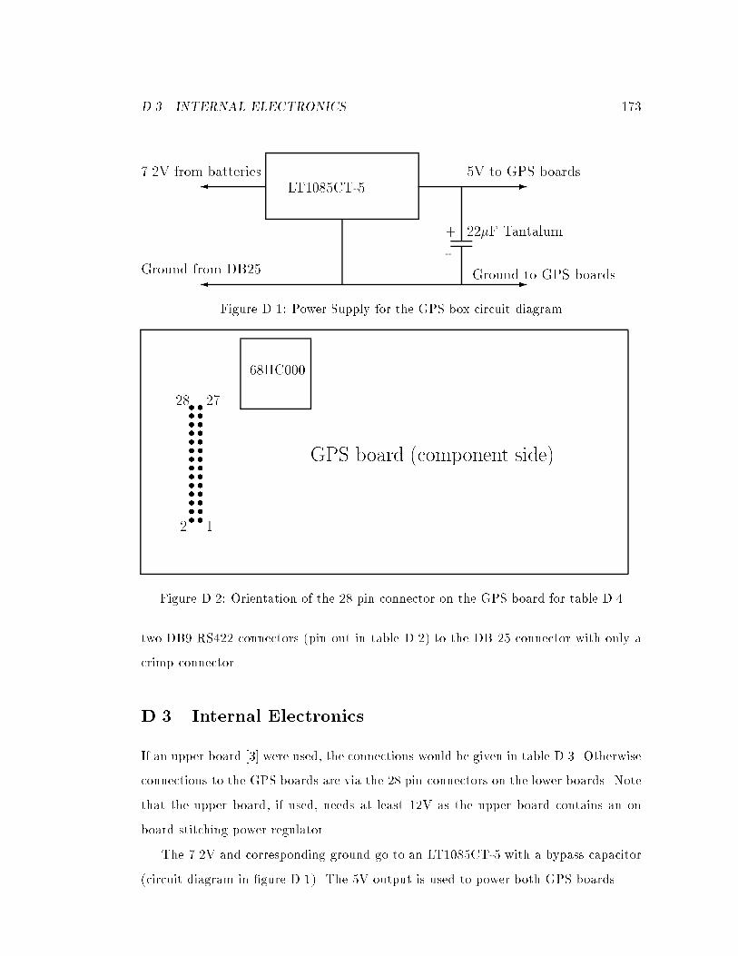
D.3. INTERNAL ELECTRONICS 173
� -
� -
LT1085CT-5
+
-
7.2V from batteries
Ground from DB25
5V to GPS boards
22�F Tantalum
Ground to GPS boards
Figure D.1: Power Supply for the GPS box circuit diagram
s ss ss ss ss ss ss ss ss ss ss ss ss ss s
28 27
68HC000
GPS board (component side)
2 1
Figure D.2: Orientation of the 28 pin connector on the GPS board for table D.4
two DB9 RS422 connectors (pin out in table D.2) to the DB 25 connector with only a
crimp connector.
D.3 Internal Electronics
If an upper board [3] were used, the connections would be given in table D.3. Otherwise
connections to the GPS boards are via the 28 pin connectors on the lower boards. Note
that the upper board, if used, needs at least 12V as the upper board contains an on
board stitching power regulator.
The 7.2V and corresponding ground go to an LT1085CT-5 with a bypass capacitor
(circuit diagram in �gure D.1). The 5V output is used to power both GPS boards.
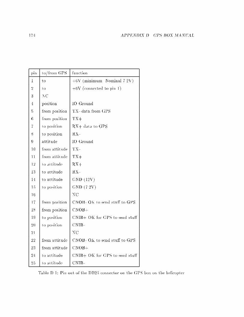
174 APPENDIX D. GPS BOX MANUAL
pin to/from GPS function
1 to +6V (minimum. Nominal 7.2V)
2 to +6V (connected to pin 1)
3 NC
4 position IO Ground
5 from position TX- data from GPS
6 from position TX+
7 to position RX+ data to GPS
8 to position RX-
9 attitude IO Ground
10 from attitude TX-
11 from attitude TX+
12 to attitude RX+
13 to attitude RX-
14 to attitude GND (12V)
15 to position GND (7.2V)
16 NC
17 from position CNOB- OK to send stu� to GPS
18 from position CNOB+
19 to position CNIB+ OK for GPS to send stu�
20 to position CNIB-
21 NC
22 from attitude CNOB- OK to send stu� to GPS
23 from attitude CNOB+
24 to attitude CNIB+ OK for GPS to send stu�
25 to attitude CNIB-
Table D.1: Pin out of the DB25 connector on the GPS box on the helicopter

D.3. INTERNAL ELECTRONICS 175
pin name to/from GPS function
1 TX- to data to be sent
2 TX+ to
3 RX+ from data from the GPS
4 RX- from
5 GND data ground
6 RTS- to request to send (IBM ready for data)
7 RTS+ to
8 CTS+ from the GPS board is ready for data
9 CTS- from
Table D.2: Pin out of the DB9 connectors going to the GPS box on the helicopter
s ss ss ss ss ss ss ss ss ss ss ss ss ss s
AAA
��
.....................
BBBBB
68HC000
GPS board (component side)
power supply
DB25
Figure D.3: Orientation of the 34 pin IDC connector on the GPS board 28 pin connector
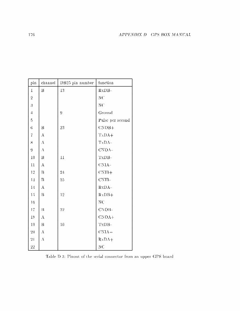
176 APPENDIX D. GPS BOX MANUAL
pin channel DB25 pin number function
1 B 13 RxDB-
2 NC
3 NC
4 9 Ground
5 Pulse per second
6 B 23 CNOB+
7 A TxDA+
8 A TxDA-
9 A CNOA-
10 B 11 TxDB-
11 A CNIA-
12 B 24 CNIB+
13 B 25 CNIB-
14 A RxDA-
15 B 12 RxDB+
16 NC
17 B 22 CNOB-
18 A CNOA+
19 B 10 TxDB-
20 A CNIA+
21 A RxDA+
22 NC
Table D.3: Pinout of the serial connector from an upper GPS board
D.4. GROUND POWER SUPPLY 177
The connections to each GPS board on the 28 pin connector consist of power, which
goes to the voltage regulator, and serial port B1, which is sent directly to the DB 25
connector.
Due to the scarcity of 28 pin IDC connectors, 34 pin connectors were used. A picture
of the connector giving orientation is given in �gure D.2, with the placing of the 34 pin
connector on it shown in �gure D.3.
D.4 Ground Power Supply
This is a box designed for use on the ground. It has two purposes in life:
� Provide about 7V for the radio transmitter
� Provide a convenient supply with on/o� switch for the ground GPS receiver
A car or motorcycle 12V battery is then typically connected to the input of this box,
and then the switched 12V output is connected to the GPS receiver, and the regulated
output to the data radio transmitter. Both can then be switched on or o� cleanly. This
box speeds up setting up time and convenience.
The simple circuit diagram is given in �gure D.4.
D.5 Supplier Information
The GPS boards come from Trimble Navigation, contact Mark Crotty, (408) 481 2221.
Trimble gave Stanford a large discount.
The LT1085CT-5 regulators are rare: practically no retailers have them. They can
be obtained most easily through Arrow Electronics (408) 441 9700, credit card line (800)
833 3557, fax (612) 946 4835. They have a $50 minimum order.
1There are two serial ports on the TANS. Port B can do everything needed.
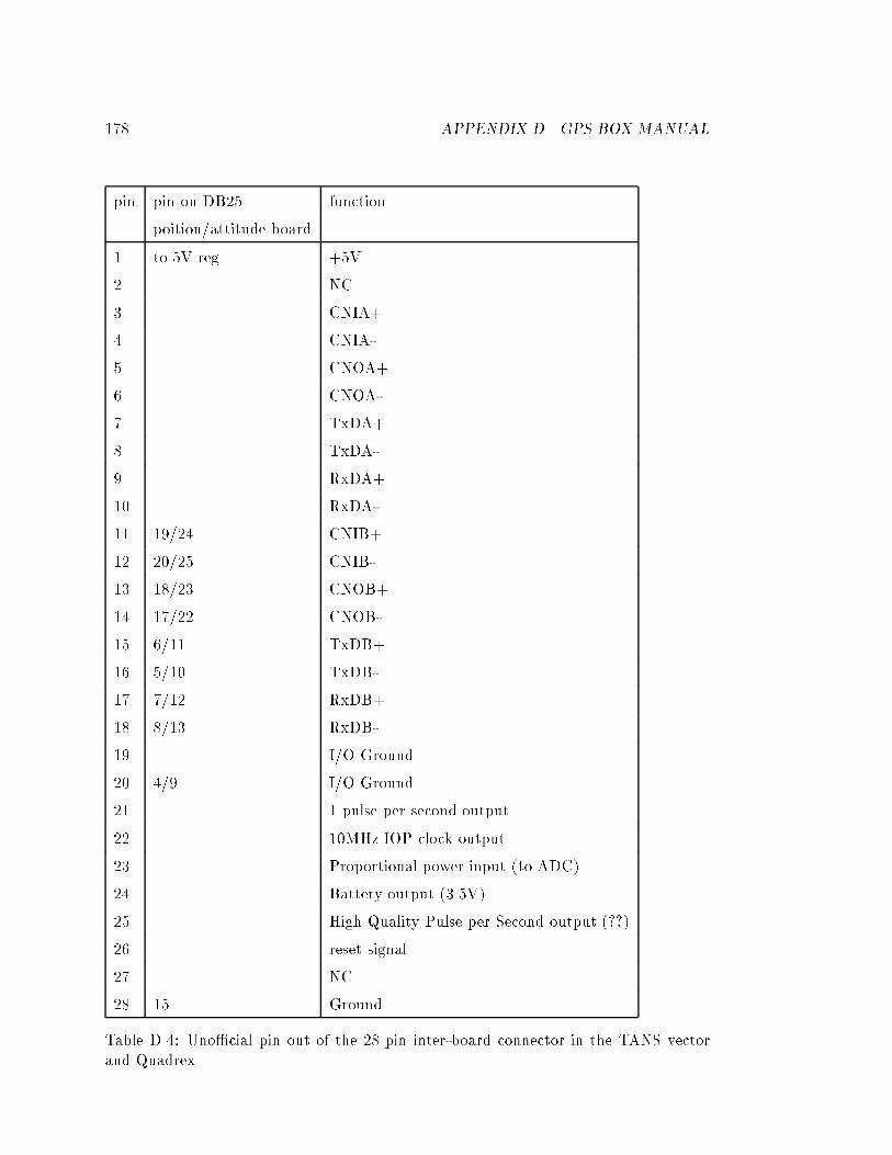
178 APPENDIX D. GPS BOX MANUAL
pin pin on DB25 function
poition/attitude board
1 to 5V reg. +5V
2 NC
3 CNIA+
4 CNIA-
5 CNOA+
6 CNOA-
7 TxDA+
8 TxDA-
9 RxDA+
10 RxDA-
11 19/24 CNIB+
12 20/25 CNIB-
13 18/23 CNOB+
14 17/22 CNOB-
15 6/11 TxDB+
16 5/10 TxDB-
17 7/12 RxDB+
18 8/13 RxDB-
19 I/O Ground
20 4/9 I/O Ground
21 1 pulse per second output
22 10MHz IOP clock output
23 Proportional power input (to ADC)
24 Battery output (3.5V)
25 High Quality Pulse per Second output (??)
26 reset signal
27 NC
28 15 Ground
Table D.4: Uno�cial pin out of the 28 pin inter-board connector in the TANS vectorand Quadrex
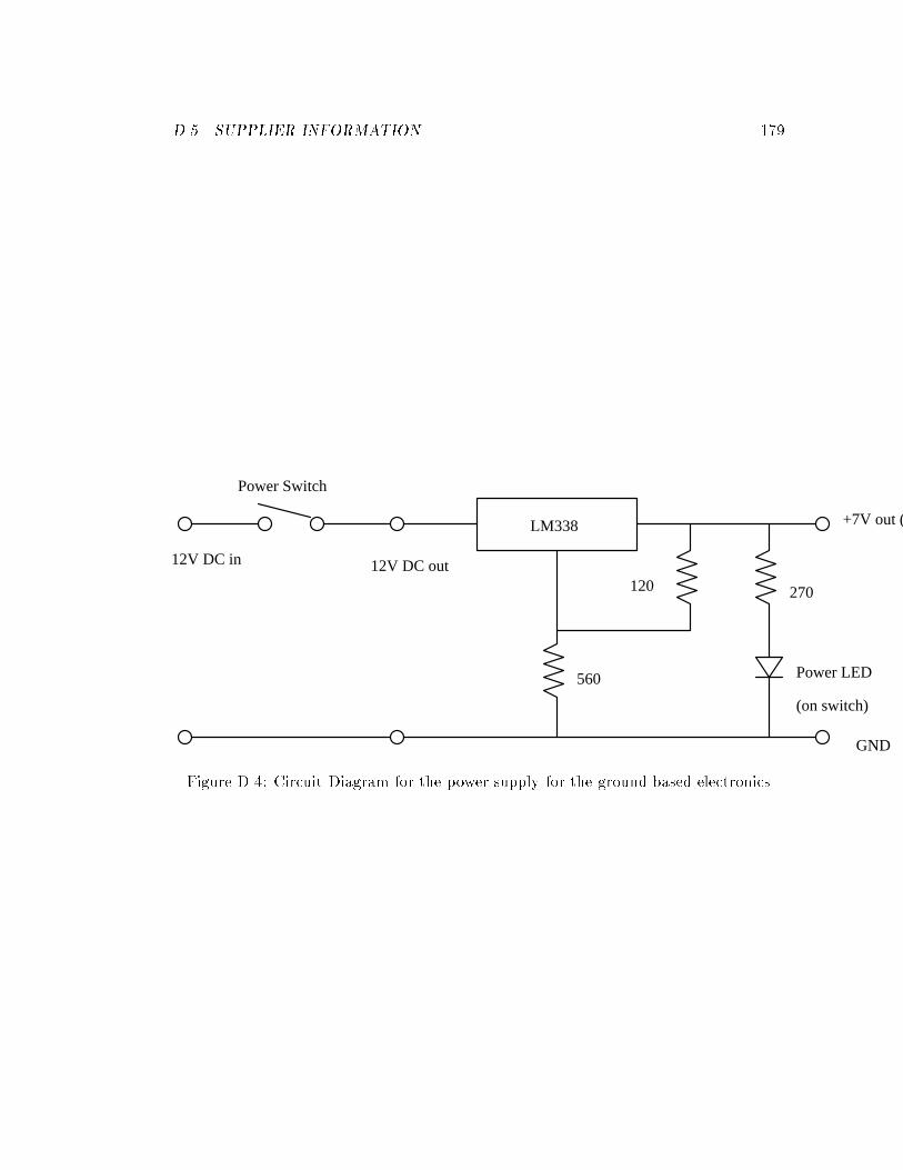
D.5. SUPPLIER INFORMATION 179
560
120 270
Power LED
(on switch)
Power Switch
GND
+7V out (
12V DC in 12V DC out
LM338
Figure D.4: Circuit Diagram for the power supply for the ground based electronics
Appendix E
GPS Program
This appendix describes the function of the program GPS , which sits logically on top of
TSR , processing phase measurements, producing position and attitude data, and using
these data to compute servo controls which are then sent to the servos through TSR .
A full description of what gets computed where and why is given in section 4.3. This
appendix contains information more useful to a person trying to modify or understand
the program.
E.1 Interface to TSR
There are three main types of communication between GPS and TSR .
� (TSR ! GPS ) Data packets from the GPS receivers, the ground station, or Con-
sole commands
� (GPS ! TSR ) Initialisation packets for the GPS receivers
� (GPS ! TSR ) LED control (indicating status).
� (GPS ! TSR ) Servo Control
� Initialising above communication
LED and servo control are performed through the normal software interrupt scheme
detailed in section B.6. Reception and transmission of GPS packets is as described in
180
E.2. PROCESSING OF PACKETS 181
section B.6.4. Whenever the callback function in GPS is invoked by TSR , a packet of
data is available. The contents of this packet are copied to a temporary storage place for
later processing (see section E.2). This is done so that the interrupt function can return
quickly, and so that the rest of the program does not have to worry about the stack
segment di�ering from the data segment which may be the case during an interrupt.
Most of this processing is done in the �les interfac.c and serbuffe.c. The �le
serbuffe.c does the bu�ering of the packets, and is the only �le in the application that
has to deal with the stack segment and the data segment not being the same.
E.2 Processing of packets
At the heart of the GPS program is a big loop which polls for new packets. Polling
may sound a little ine�cient: why poll when one could interrupt? The main reason
is that due to the non-multitasking structure of MS-DOS, triggering a time consuming
calculation inside an interrupt is di�cult without a polling loop. Fortunately this is not
a problem as polling for packets is not as time critical as polling for individual bytes,
and that usually one doesn't actually want to interrupt existing processing when a new
packet comes in.
The main loop also checks the keyboard for a `q' character to see if GPS should
quit, or for various other characters to do various debugging commands. These are not
documented here as they change often and are not interesting.
When a packet is received in the polling loop, the packet is checked to see if it should
be displayed. After that, the packet is passed to a great big gps data structure into which
the information in the packet is inserted in a structured manner. This structure keeps
track of the state of the world as far as is knows by the GPS receivers.
If the busy loop runs out of packets to process, GPS checks to see if anything signi�-
cant has happened to the GPS world structure since GPS last did a computation. If so,
a new position, attitude and/or control computation is performed as appropriate.
This may sound overly complex, but has the features of
� Returning from the interrupt routine quickly.
182 APPENDIX E. GPS PROGRAM
� Dealing with queues of packets quickly: if GPS is getting new packets faster than
GPS can process every packet (which doesn't happen in practice on the CPU we
are using currently), GPS ignores old packets and only deals with the latest data.
� GPS responds to packets with computations in practice very rapidly
E.3 Source �les
GPS is made from many source �les. They are listed as follows:
attcomp.c Computes attitude from phases and attitude integers.
attcomp.h Structures used in attcomp.c
control.c Computes control values.
environ.c Some generally useful utilities.
environ.h Prototypes for useful utilities.
gps.c Manage the GPS world model and compute GPS position.
gps.h The GPS world structures.
gr.c Creates a graphic display of the helicopter status.
helicont.h Interconverts raw servo commands and physical units.
interfac.c Communicates with TSR and the user.
lookup.h The lookup table to get a �rst approximation to the minimum of equation
(2.23).
mat math.c Some matrix routines used in gps.c
mat math.h Prototypes for functions in mat math.c
matrix.c Some matrix functions used in attcomp.c
matrix.h Prototypes for functions in matrix.c
E.4. C++ CLASSES 183
nogr.c Creates a text display of helicopter status (c.f. gr.c).
radiocom.h Contains the gains structure uplinked from the base station.
serbu�e.c Bu�ers the GPS packets
serbu�e.h The interface between serbu�e.c and interfac.c
service.h The interface between tsr.c and interfac.c
setup.h Calculates checksum on gains packet. Also used by remote.exe.
swabtype.h Data types to safely manage the di�erence between big-endian and little-
endian architectures.
tans.h Packet de�nitions from the TANS.
E.4 C++ Classes
This section contains a brief description of the purpose of most of the classes used in
this program. They will de divided up by their source.
E.4.1 Data Swabbing
The packets coming from the TANS receivers contain multibyte values in the opposite
order in memory to the order expected by the IBM. Through the explicit type conversion
operators of C++ it is possible to make data types INTEGER, LONG, SINGLE and
DOUBLE which are stored in memory in the format used by the TANS, and which
can be implicitly converted to an IBM usable type in calculations. Having them as
an explicit type prevents mistakes of omission of swabbing. These types are de�ned in
swabtype.h and are used in tans.h.
E.4.2 General Utility
The �le environ.h contains de�nitions for a few useful classes that make the program a
little easier to use.

184 APPENDIX E. GPS PROGRAM
env Replaces a default string by an environment variable if the environment variable
is set.
print to me Opens a �le pointer at the start of the program if given a non-null ini-
tialisation. Typically used for postprocessing with a �lename coming from env
above.
no numerror Prevents normal behavious of numeric errors (crash the program) during
the scope of a variable of this type. If invoked with arguement(s), check for errors
and print out useful diagnostics. If invoked with no arguments, ignore errors. The
former is useful for debugging; the latter is useful during a sanity check of an
incoming packet; a corrupted packet does not cause the program to crash.
E.4.3 Matrix
A matrix class has been de�ned in matrix.c and matrix.h. This class is designed and
tuned for ease of use and e�ciency of operation for the types of operations used in
attitude computation.
E.4.4 Attitude computation
There are a large number of variables needed in the attitude computation process.
Rather than send all as parameters or have global variables, these variables are kept
in local structures. Some additional useful classes are also de�ned. Following are the
classes de�ned in attcomp.h.
quaternion A unit magnitude quaternion used for convenient attitude de�nition and
manipulation.
direction A three component vector used to indicate a direction.
rotation matrix A three by three rotation matrix used to represent a rotation for
e�cient computation.
baselines A structure encapsulating the surveyed locations and line biases of the four
GPS antennas.
E.4. C++ CLASSES 185
att basic Basic information needed for both attitude computation and integer resolu-
tion
intsolve Everything required to perform attitude integer resolution.
attsolve Everything required to perform attitude computation.
E.4.5 GPS world model
The GPS world model is fairly complex, containing a variety of heterogeneous data.
These data are collected in one overall structure, gps, with detailed sub-objects to make
it easy to maintain. The following classes are de�ned in gps.h:
history A general, template class for maintianing a time history of some type of data.
sv Measurements on a single satellite at a single receiver with a single antenna.
posn packet Measurements of a single receiver.
posn coarse Pseudorange GPS position information.
los The line of sight vector for a single satellite.
losbuf Information needed to interpolate or extrapolate line of sight vectors for any
time for one satellite.
los store All knowledge of satellite line of sight vectors.
posn history History of receiverd phase data for one receiver. Used to maintain inte-
gers.
coarse histroy History of pseudorange position data. Used for clock bias measure-
ments and stability check.
time manager Manage time for sanity checks for received phase data and deduction
of the uppermost bits of a time given the lowermost bits.
att sv Measurements of a single satellite at four antennas with one receiver.
186 APPENDIX E. GPS PROGRAM
att meas One measurement for all satellites at four antennas with one receiver.
att history A time history of pahse measurements at four antennas with one receiver.
Used for integer maintenance and resolution.
match svs A class with phases from the ground and helicopter receivers matched ready
for position computation.
position A computed position.
gps The GPS world model, containing all previous structures.
E.4.6 Control
For ease of manipulation, a few structures are used in the control system:
gains A list of the gains used in the control system.
packet gains The packet sent from the basestation containing the gains. Includes a
checksum and the destination.
rotated position The current position and velocity error in body coordinates together
with the current attitude. Used together with gains to produce the control signals.
E.5 Debugging �les and postprocessing
Postprocessing is performed by running GPS with various environment variables set to
the names of �les requested. A list of the environment variables and the contents of the
�les produced if the environment variable is set follows:
GPS ATTSOLVE FILE GPS attitude solution and debugging information.
GPS BPHI FILE B and � values for which equation (2.23) needs to be solved. Used
to create �gure 2.7.
GPS ID FILE Some information useful for system identi�cation.
GPS INTSOLVE FILE Debugging information for integer resolution.
E.5. DEBUGGING FILES AND POSTPROCESSING 187
GPS LOS FILE Debugging information of line of sight vectors.
GPS POSN FILE GPS Position calculations.
GPS SNR FILE Information on SNRs for satellites.
GPS VEL FILE GPS velocity calculation.
GPS XMS FILE Information saved explicitly by GPS to XMS during the ight.
Appendix F
List of Acronyms
This appendix contains a list of the acronyms used in this thesis which may be unfamiliar
to some of the readers.
486 An Intel microprocessor
68HC11 A Motorola microcontoller
AUVS Association for Unmanned Vehicle Systems
cConversion factor between time and distance; the speed of
light; 1
C/A Coarse Acquisition. The most commonly used GPS code.
FIFO First In First Out. A bu�er.
GP-BGravity Proble B. A large project at Stanford that also
works with GPS
GPS Global Positioning System
188
189
HC11 68HC11
L1 1.575420.0 GHz; GPS C/A carrier frequency
MS DOSMicroSoft Disk Operating System. A common operating
system for IBM PC compatible computers.
P P code is a GPS signal that is more precise than C/A code
PDProportional Di�erential. A type of feedback consisting of
a signal proportional to x and a signal proportional to _x.
PRN Pseudo Random Noise
PWMPulse Width Modulated. A signal whose value is determined
by the length of a pulse
RAM Random Access Memory. Fast, solid state storage.
RC Remote/Radio Controlled (teleoperated)
RS232 A common serial communications standard
RS422A serial communications standard less common than RS232
but more reliable.
SA Selective Availability
SCISerial Communications Interface. A standard serial port on
the 68HC11
SPISerial Peripheral Interface. A less standard serial port on
the 68HC11
190 APPENDIX F. LIST OF ACRONYMS
SV Space Vehicle. Synonym for satelite
TANS
Trimble Advanced Navigation System. The gps receiver
hardware, operating with modi�ed EPROMS provided by
the GP-B lab at Stanford
TSR
Terminate and Stay Resident. A type of program under MS
DOS that returns control to the system, but leaves the code
resident in memory activated by interrupts.
US DoDUnited States Department of Defense; organisation that put
up the GPS satelites and maintain selective availability
Bibliography
[1] PCA-6143 Half-size All-in-One 486SX/DX/DX2 CPU Card With Flash/ROM Disk
User's Manual. 750 East Arques Avenue, Sunnyvale, CA 94086,U.S.A.
[2] PCL-743 Dual Port RS-422/RS-485 Interface Card User's Manual. 750 East Ar-
ques Avenue, Sunnyvale, CA 94086,U.S.A., rev. a2 edition, Dec. 1989.
[3] TANS VECTOR Four-Antenna GPS Attitude Determination System SPECIFICA-
TION AND USER'S MANUAL. 645 North Mary Avenue Sunnyvale CA 94086,
revision a edition, June 1993.
[4] J. L. Armstrong, B. O. D�acker, S. R. Virding, and M. C. Williams. Implement-
ing a functional language for highly parallel real time applications. In Software
Engineering for Telecommunication Systems and Services, pages 157{163, 1992.
[5] Albert Benveniste and Paul Le Guernic. Hybrid dynamical systems theory and the
signal language. IEEE Transactions on Automatic Control, 35(5):535{546, May
1990.
[6] K M Black, R G Martinez, W Page, and J Fitzer. Evolution and design of the 1993
university of texas at arlington autonomous aerial vehicle. In Proceedings, June
1993.
[7] R Brown and P Ward. A gps receiver with built-in precision pointing capability.
In IEEE PLANS, pages 83{93, March 1990.
191
192 BIBLIOGRAPHY
[8] Clark E Cohen, Boris Pervan, H. Stewart Cobb, Dave Lawrence, J. David Powell,
and Bradford W. Parkinson. Real-time cycle ambiguity resolution using a pseudo-
lite for precision landing of aircraft with gps. In Second International Symposium
on Di�erential Satellite Navigation Systems, March 30-April 2 1993. Amsterdam.
[9] Clark Emerson Cohen. Attitude Determination Using GPS. PhD thesis, Stan-
ford University, Department of Aeronautics and Astronautics, Stanford, CA 94305,
December 1992.
[10] Frederick G Edwards and Peter V W Loomis. Civil Helicopter Flight Operations
Using Di�erential GPS, volume 3, pages 173{193. Institute of Navigation, Wash-
ington D.C., 1986.
[11] K. Ferguson, J Kosmalska, M Kuhl, J M Eichner, K Kepski, and R Abtahi. In
IEEE PLANS, March 1991.
[12] F. Van Graas and M. Braasch. Gps interferometric attitude and heading determi-
nation: initial ight test results. Navigation. Journal of the Institute of Navigation,
38(4):297{316, 1991-1992.
[13] Paul Hudak. Conception, evolution and application of functional programming
languages. ACM Computing Surveys, 21(3):359{411, 1989.
[14] P. Y. C. Hwang. Kinematic gps: resolving integer ambiguities on the y. In IEEE
PLANS, pages 579{586, March 1990.
[15] M. Anthony Lewis, Andrew H Fagg, and George A Bekey. The USC autonomous
ying vehicle: An experiment on real-time behavior control. In IEEE 1993 Inter-
national Converence on Robotics and Automation, pages 422{429, May 1993.
[16] P. V. W. Loomis. A kinematic gps double di�erencing algorithm. 13-17 March
1989.
[17] G. Lu, M E Cannon, G Lachapelle, and P Kielland. Attitude determination us-
ing dedicated and nondedicated multiantenna gps sensors. IEEE Transactions on
Aerospace and Electronic Systems, 30(4):1053{1058, Oct. 1994.
BIBLIOGRAPHY 193
[18] Paul Y montgomery, Hirohiko Uematsu, and Bradford W Parkinson. Analysis of
angular velocity determination using GPS. Sep 1994. Salt Lake City.
[19] H. S. Satz, D. B. Cox, R. L. Beard, and G. P. Landis. Gps inertial attitude
estimation via carrier accumulated-phase measurements. Navigation. Journal of
the Institute of Navigation, 38(3):273{284, 1991.
[20] S. Schneider. Experiments in the Dynamic and Strategic Control of Cooperating
Manipulators. PhD thesis, Stanford University, Stanford, CA 94305, September
1989. Also published as SUDAAR 586.
[21] V W Spinney. Applications of the global positioning system as an attitude reference
for near earth uses. Navigation. Journal of the Institute of Navigation, April 1976.
[22] Boleslaw K. Szymanski, editor. Parallel Functional Languages and Compilers.
ACM Press, New York, New York, 1991.
[23] S. ShouHan Wang and A. K. Uht. Ideograph/ideogram: framework/hardware for
eager evaluation. Micro, 23:125{134, 1990.
[24] K. R. Zimmerman and R. H. Cannon Jr. GPS-Based Control for Space Vehicle
Rendezvous. In Proceedings of the ASCE: Robotics for Challenging Environments,
Albuquerque NM, February 28 - March 3 1994.