Variational Denoising Network: Toward Blind NoiseModeling and Removal

Zongsheng Yue1,2, Hongwei Yong2, Qian Zhao1, Lei Zhang2,3, Deyu Meng4,1,*

1 School of Mathematics and Statistics, Xi’an Jiaotong University, Shaanxi, China2Department of Computing, Hong Kong Polytechnic University, Kowloon, Hong Kong

3DAMO Academy, Alibaba Group, Shenzhen, China4Faculty of Information Technology, The Macau University of Science and Technology, Macau, China

*Corresponding author: dymeng@mail.xjtu.edu.cn

Abstract

Blind image denoising is an important yet very challenging problem in computervision due to the complicated acquisition process of real images. In this work wepropose a new variational inference method, which integrates both noise estimationand image denoising into a unique Bayesian framework, for blind image denoising.Specifically, an approximate posterior, parameterized by deep neural networks, ispresented by taking the intrinsic clean image and noise variances as latent variablesconditioned on the input noisy image. This posterior provides explicit parametricforms for all its involved hyper-parameters, and thus can be easily implementedfor blind image denoising with automatic noise estimation for the test noisy image.On one hand, as other data-driven deep learning methods, our method, namelyvariational denoising network (VDN), can perform denoising efficiently due toits explicit form of posterior expression. On the other hand, VDN inherits theadvantages of traditional model-driven approaches, especially the good general-ization capability of generative models. VDN has good interpretability and canbe flexibly utilized to estimate and remove complicated non-i.i.d. noise collectedin real scenarios. Comprehensive experiments are performed to substantiate thesuperiority of our method in blind image denoising.

1 IntroductionImage denoising is an important research topic in computer vision, aiming at recovering the underlyingclean image from an observed noisy one. The noise contained in a real noisy image is generallyaccumulated from multiple different sources, e.g., capturing instruments, data transmission media,image quantization, etc. [40]. Such complicated generation process makes it fairly difficult to accessthe noise information accurately and recover the underlying clean image from the noisy one. Thisconstitutes the main aim of blind image denoising.

There are two main categories of image denoising methods. Most classical methods belong to the firstcategory, mainly focusing on constructing a rational maximum a posteriori (MAP) model, involvingthe fidelity (loss) and regularization terms, from a Bayesian perspective [6]. An understanding for datageneration mechanism is required for designing a rational MAP objective, especially better imagepriors like sparsity [3], low-rankness [16, 50, 42], and non-local similarity [9, 27]. These methodsare superior mainly in their interpretability naturally led by the Bayesian framework. They, however,still exist critical limitations due to their assumptions on both image prior and noise (generally i.i.d.Gaussian), possibly deviating from real spatially variant (i.e.,non-i.i.d.) noise, and their relatively lowimplementation speed since the algorithm needs to be re-implemented for any new coming image.Recently, deep learning approaches represent a new trend along this research line. The main idea is tofirstly collect large amount of noisy-clean image pairs and then train a deep neural network denoiseron these training data in an end-to-end learning manner. This approach is especially superior in its

33rd Conference on Neural Information Processing Systems (NeurIPS 2019), Vancouver, Canada.

effective accumulation of knowledge from large datasets and fast denoising speed for test images.They, however, are easy to overfit to the training data with certain noisy types, and still could not begeneralized well on test images with unknown but complicated noises.

Thus, blind image denoising especially for real images is still a challenging task, since the realnoise distribution is difficult to be pre-known (for model-driven MAP approaches) and hard to becomprehensively simulated by training data (for data-driven deep learning approaches).

Against this issue, this paper proposes a new variational inference method, aiming at directly inferringboth the underlying clean image and the noise distribution from an observed noisy image in a uniqueBayesian framework. Specifically, an approximate posterior is presented by taking the intrinsic cleanimage and noise variances as latent variables conditioned on the input noisy image. This posteriorprovides explicit parametric forms for all its involved hyper-parameters, and thus can be efficientlyimplemented for blind image denoising with automatic noise estimation for test noisy images.

In summary, this paper mainly makes following contributions: 1) The proposed method is capableof simultaneously implementing both noise estimation and blind image denoising tasks in a uniqueBayesian framework. The noise distribution is modeled as a general non-i.i.d. configurations withspatial relevance across the image, which evidently better complies with the heterogeneous realnoise beyond the conventional i.i.d. noise assumption. 2) Succeeded from the fine generalizationcapability of the generative model, the proposed method is verified to be able to effectively estimateand remove complicated non-i.i.d. noises in test images even though such noise types have neverappeared in training data, as clearly shown in Fig. 3. 3) The proposed method is a generative approachoutputted a complete distribution revealing how the noisy image is generated. This not only makesthe result with more comprehensive interpretability beyond traditional methods purely aiming atobtaining a clean image, but also naturally leads to a learnable likelihood (fidelity) term accordingto the data-self. 4) The most commonly utilized deep learning paradigm, i.e., taking MSE as lossfunction and training on large noisy-clean image pairs, can be understood as a degenerated form ofthe proposed generative approach. Their overfitting issue can then be easily explained under thisvariational inference perspective: these methods intrinsically put dominant emphasis on fitting thepriors of the latent clean image, while almost neglects the effect of noise variations. This makes themincline to overfit noise bias on training data and sensitive to the distinct noises in test noisy images.

The paper is organized as follows: Section 2 introduces related work. Sections 3 presents the proposedfull Bayesion model, the deep variational inference algorithm, the network architecture and somediscussions. Section 4 demonstrates experimental results and the paper is finally concluded.

2 Related WorkWe present a brief review for the two main categories of image denoising methods, i.e., model-drivenMAP based methods and data-driven deep learning based methods.

Model-driven MAP based Methods: Most classical image denoising methods belong to this cate-gory, through designing a MAP model with a fidelity/loss term and a regularization one deliveringthe pre-known image prior. Along this line, total variation denoising [37], anisotropic diffusion [31]and wavelet coring [38] use the statistical regularities of images to remove the image noise. Later,the nonlocal similarity prior, meaning many small patches in a non-local image area possess similarconfigurations, was widely used in image denoising. Typical ones include CBM3D [11] and non-localmeans [9]. Some dictionary learning methods [16, 13, 42] and Field-of-Experts (FoE) [36], also re-vealing certain prior knowledge of image patches, had also been attempted for the task. Several otherapproaches focusing on the fidelity term, which are mainly determined by the noise assumption ondata. E.g., Mulitscale [23] assumed the noise of each patch and its similar patches in the same imageto be correlated Gaussian distribution, and LR-MoG [30, 48, 50], DP-GMM [44] and DDPT [49]fitted the image noise by using Mixture of Gaussian (MoG) as an approximator for noises.

Data-driven Deep Learning based Methods: Instead of pre-setting image prior, deep learningmethods directly learn a denoiser (formed as a deep neural network) from noisy to clean oneson a large collection of noisy-clean image pairs. Jain and Seung [19] firstly adopted a five layerconvolution neural network (CNN) for the task. Then some auto-encoder based methods [41, 2] wereapplied. Meantime, Burger et al. [10] achieved the comparable performance with BM3D using plainmulti-layer perceptron (MLP). Zhang et al. [45] further proposed the denoising convolution network(DnCNN) and achieved state-of-the-art performance on Gaussian denoising tasks. Mao et al. [29]proposed a deep fully convolution encoding-decoding network with symmetric skip connection. Tai

2

et al. [39] preposed a very deep persistent memory network (MemNet) to explicitly mine persistentmemory through an adaptive learning process. Recently, NLRN [25], N3Net [33] and UDNet [24]all embedded the non-local property of image into DNN to facilitate the denoising task. In order toboost the flexibility against spatial variant noise, FFDNet [46] was proposed by pre-evaluating thenoise level and inputting it to the network together with the noisy image. Guo et al. [17] and Brookset al. [8] both attempted to simulate the generation process of the images in camera.

3 Variational Denoising Network for Blind Noise ModelingGiven training set D = {yj ,xj}nj=1, where yj ,xj denote the jth training pair of noisy and theexpected clean images, n represents the number of training images, our aim is to construct a variationalparametric approximation to the posterior of the latent variables, including the latent clean imageand the noise variances, conditioned on the noisy image. Note that for the noisy image y, its trainingpair x is generally a simulated “clean” one obtained as the average of many noisy ones taken undersimilar camera conditions [4, 1], and thus is always not the exact latent clean image z. This explicitparametric posterior can then be used to directly infer the clean image and noise distribution fromany test noisy image. To this aim, we first need to formulate a rational full Bayesian model of theproblem based on the knowledge delivered by the training image pairs.

3.1 Constructing Full Bayesian Model Based on Training DataDenote y = [y1, · · · , yd]T and x = [x1, · · · , xd]T as any training pair in D, where d (width*height)is the size of a training image1. We can then construct the following model to express the generationprocess of the noisy image y:

yi ∼ N (yi|zi, σ2i ), i = 1, 2, · · · , d, (1)

where z ∈ Rd is the latent clean image underlying y, N (·|µ, σ2) denotes the Gaussian distributionwith mean µ and variance σ2. Instead of assuming i.i.d. distribution for the noise as conventional [28,13, 16, 42], which largely deviates the spatial variant and signal-depend characteristics of the realnoise [46, 8], we models the noise as a non-i.i.d. and pixel-wise Gaussian distribution in Eq. (1).

The simulated “clean” image x evidently provides a strong prior to the latent variable z. Accordinglywe impose the following conjugate Gaussian prior on z:

zi ∼ N (zi|xi, ε20), i = 1, 2, · · · , d, (2)where ε0 is a hyper-parameter and can be easily set as a small value.

Besides, for σ2 = {σ21 , σ

22 , · · · , σ2

d}, we also introduce a rational conjugate prior as follows:

σ2i ∼ IG

(σ2i |p2

2− 1,

p2ξi2

), i = 1, 2, · · · , d, (3)

where IG(·|α, β) is the inverse Gamma distribution with parameter α and β, ξ = G((y − x)2; p

)represents the filtering output of the variance map (y − x)2 by a Gaussian filter with p× p window,and y, x ∈ Rh×w are the matrix (image) forms of y, x ∈ Rd, respectively. Note that the mode ofabove IG distribution is ξi [6, 43], which is a approximate evaluation of σ2

i in p× p window.

Combining Eqs. (1)-(3), a full Bayesian model for the problem can be obtained. The goal then turnsto infer the posterior of latent variables z and σ2 from noisy image y, i.e., p(z,σ2|y).

3.2 Variational Form of PosteriorWe first construct a variational distribution q(z,σ2|y) to approximate the posterior p(z,σ2|y) ledby Eqs. (1)-(3). Similar to the commonly used mean-field variation inference techniques, we assumeconditional independence between variables z and σ2, i.e.,

q(z,σ2|y) = q(z|y)q(σ2|y). (4)Based on the conjugate priors in Eqs. (2) and (3), it is natural to formulate variational posterior formsof z and σ2 as follows:

q(z|y) =d∏i

N (zi|µi(y;WD),m2i (y;WD)), q(σ

2|y) =d∏i

IG(σ2i |αi(y;WS), βi(y;WS)), (5)

1We use j (= 1, · · · , n) and i (= 1, · · · , d) to express the indexes of training data and data dimension,respectively, throughout the entire paper.

3

𝝁 𝒎𝟐

𝜶 𝜷

𝐷𝑘𝑙(𝑞(𝒛|𝒚)||𝑝 𝒛 )

𝐷𝑘𝑙(𝑞(𝝈2|𝒚)||𝑝 𝝈2 )

𝐸𝑞(𝑧,𝜎2)[log 𝑝 𝒚 𝒛, 𝝈2 ] ℒ(𝒛, 𝝈2; 𝒚)

D-Net: Denoising Network

S-Net: Sigma Network

Variational Posterior:

𝑞 𝒛 𝒚 = 𝒩 𝒛 𝝁,𝒎2

𝑞 𝝈2 𝒚 = 𝐼𝐺(𝝈2|𝜶, 𝜷)

𝒚

𝒚

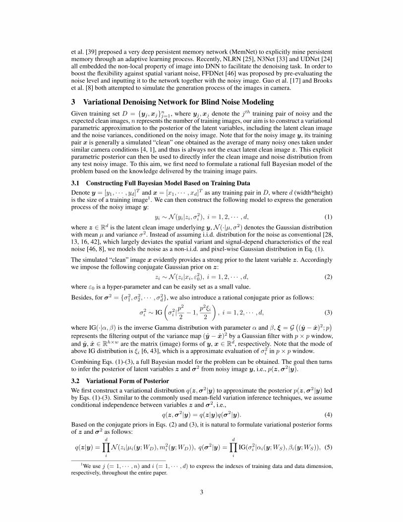
Figure 1: The architecture of the proposed deep variational inference network. The red solid lines denote theforward process, and the blue dotted lines mark the gradient flow direction in the BP algorithm.

where µi(y;WD) and m2i (y;WD) are designed as the prediction functions for getting posterior

parameters of latent variable z directly from y. The function is represented as a network, calleddenoising network or D-Net, with parameters WD. Similarly, αi(y;WS) and βi(y;WS) denote theprediction functions for evaluating posterior parameters of σ2 from y, where WS represents theparameters of the network, called Sigma network or S-Net. The aforementioned is illustrated in Fig. 1.Our aim is then to optimize these network parameters WD and WS so as to get the explicit functionsfor predicting clean image z as well as noise knowledge σ2 from any test noisy image y. A rationalobjective function with respect to WD and WS is thus necessary to train both the networks.

Note that the network parameters WD and WS are shared by posteriors calculated on all trainingdata, and thus if we train them on the entire training set, the method is expected to induce the generalstatistical inference insight from noisy image to its underlying clean image and noise level.

3.3 Variational Lower Bound of Marginal Data LikelihoodFor notation convenience, we simply write µi(y;WD), m2

i (y;WD), αi(y;WS), βi(y;WS) as µi,m2i , αi, βi in the following calculations. For any noisy image y and its simulated “clean” image x in

the training set, we can decompose its marginal likelihood as the following form [7]:

log p(y; z,σ2) = L(z,σ2;y) +DKL

(q(z,σ2|y)||p(z,σ2|y)

), (6)

whereL(z,σ2;y) = Eq(z,σ2|y)

[log p(y|z,σ2)p(z)p(σ2)− log q(z,σ2|y)

], (7)

Here Ep(x)[f(x)] represents the exception of f(x) w.r.t. stochastic variable x with probability densityfunction p(x). The second term of Eq. (6) is a KL divergence between the variational approximateposterior q(z,σ2|y) and the true posterior p(z,σ2|y) with non-negative value. Thus the first termL(z,σ2;y) constitutes a variational lower bound on the marginal likelihood of p(y|z,σ2), i.e.,

log p(y; z,σ2) ≥ L(z,σ2;y). (8)

According to Eqs. (4), (5) and (7), the lower bound can then be rewritten as:

L(z,σ2;y) = Eq(z,σ2|y)[log p(y|z,σ2)

]−DKL (q(z|y)||p(z))−DKL

(q(σ2|y)||p(σ2)

). (9)

It’s pleased that all the three terms in Eq (9) can be integrated analytically as follows:

Eq(z,σ2|y)[log p(y|z,σ2)

]=

d∑i=1

{− 1

2log 2π − 1

2(log βi − ψ(αi))−

αi2βi

[(yi − µi)2 +m2

i

] }, (10)

DKL (q(z|y)||p(z)) =

d∑i=1

{ (µi − xi)2

2ε20+

1

2

[m2i

ε20− log

m2i

ε20− 1

]}, (11)

4

DKL(q(σ2|y)||p(σ2)

)=

d∑i=1

{(αi −

p2

2+ 1

)ψ(αi) +

[log Γ

(p2

2− 1

)− log Γ(αi)

]+

(p2

2− 1

)(log βi − log

p2ξi2

)+ αi

(p2ξi2βi− 1

)}, (12)

where ψ(·) denotes the digamma function. Calculation details are listed in supplementary material.

We can then easily get the expected objective function (i.e., a negtive lower bound of the marginallikelihood on entire training set) for optimizing the network parameters of D-Net and S-Net as follows:

minWD,WS

−n∑j=1

L(zj ,σ2j ;yj). (13)

3.4 Network LearningAs aforementioned, we use D-Net and S-Net together to infer the variational parameters µ,m2 andα, β from the input noisy image y, respectively, as shown in Fig. 1. It is critical to consider howto calculate derivatives of this objective with respect to WD,WS involved in µ, m2, α and β tofacilitate an easy use of stochastic gradient varitional inference. Fortunately, different from otherrelated variational inference techniques like VAE [22], all three terms of Eqs. (10)-(12) in the lowerbound Eq. (9) are differentiable and their derivatives can be calculated analytically without the needof any reparameterization trick, largely reducing the difficulty of network training.

At the training stage of our method, the network parameters can be easily updated with backprop-agation (BP) algorithm [15] through Eq. (13). The function of each term in this objective can beintuitively explained: the first term represents the likelihood of the observed noisy images in trainingset, and the last two terms control the discrepancy between the variational posterior and the corre-sponding prior. During the BP training process, the gradient information from the likelihood term ofEq. (10) is used for updating both the parameters of D-Net and S-Net simultaneously, implying thatthe inference for the latent clean image z and σ2 is guided to be learned from each other.

At the test stage, for any test noisy image, through feeding it into D-Net, the final denoising result canbe directly obtained by µ. Additionally, through inputting the noisy image to the S-Net, the noisedistribution knowledge (i.e., σ2) is easily inferred. Specifically, the noise variance in each pixel canbe directly obtained by using the mode of the inferred inverse Gamma distribution: σ2

i = βi

(αi+1) .

3.5 Network ArchitectureThe D-Net in Fig. 1 takes the noisy image y as input to infer the variational parameters µ andm2 in q(z|y) of Eq. (5), and performs the denoising task in the proposed variational inferencealgorithm. In order to capture multi-scale information of the image, we use a U-Net [35] with depth4 as the D-Net, which contains 4 encoder blocks ([Conv+ReLU]×2+Average pooling), 3 decoderblocks (Transpose Conv+[Conv+ReLU]×2) and symmetric skip connection under each scale. Forparameter µ, the residual learning strategy is adopted as in [45], i.e., µ = y + f(y;WD), wheref(·;WD) denotes the D-Net with parameters WD. As for the S-Net, which takes the noisy imagey as input and outputs the predicted variational parameters α and β in q(σ2|y) of Eq (5), we usethe DnCNN [45] architecture with five layers, and the feature channels of each layer is set as 64.It should be noted that our proposed method is a general framework, most of the commonly usednetwork architectures [46, 34, 24, 47] in image restoration can also be easily substituted.

3.6 Some DiscussionsIt can be seen that the proposed method succeeds advantages of both model-driven MAP and data-driven deep learning methods. On one hand, our method is a generative approach and possessesfine interpretability to the data generation mechanism; and on the other hand it conducts an explicitprediction function, facilitating efficient image denoising as well as noise estimation directly throughan input noisy image. Furthermore, beyond current methods, our method can finely evaluate andremove non-i.i.d. noises embedded in images, and has a good generalization capability to imageswith complicated noises, as evaluated in our experiments. This complies with the main requirementof the blind image denoising task.

If we set the hyper-parameter ε20 in Eq.(2) as an extremely small value close to 0, it is easy to seethat the objective of the proposed method is dominated by the second term of Eq. (10), which makes

5

(a)

(d1)

(d2)

(c1)

(c2)

(b1)

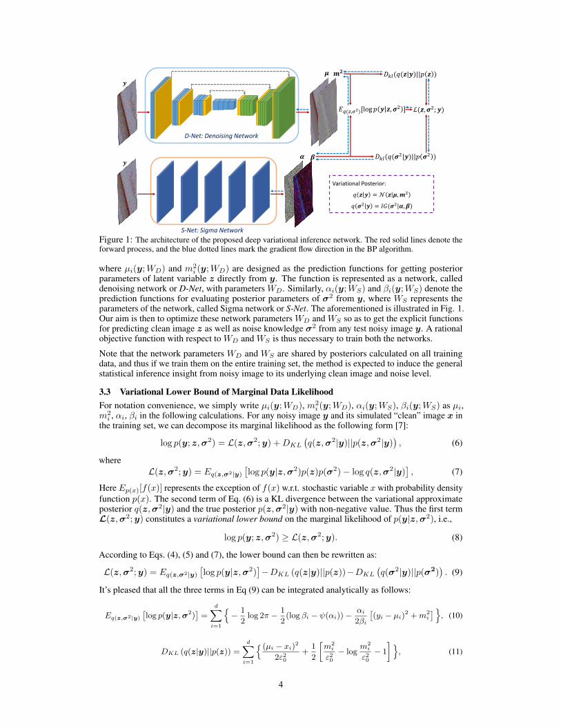
(b2)Figure 2: (a) The spatially variant mapM for noise generation in training data. (b1)-(d1): Three differentMson testing data in Cases 1-3. (b2)-(d2): Correspondingly predictedMs by our method on the testing data.

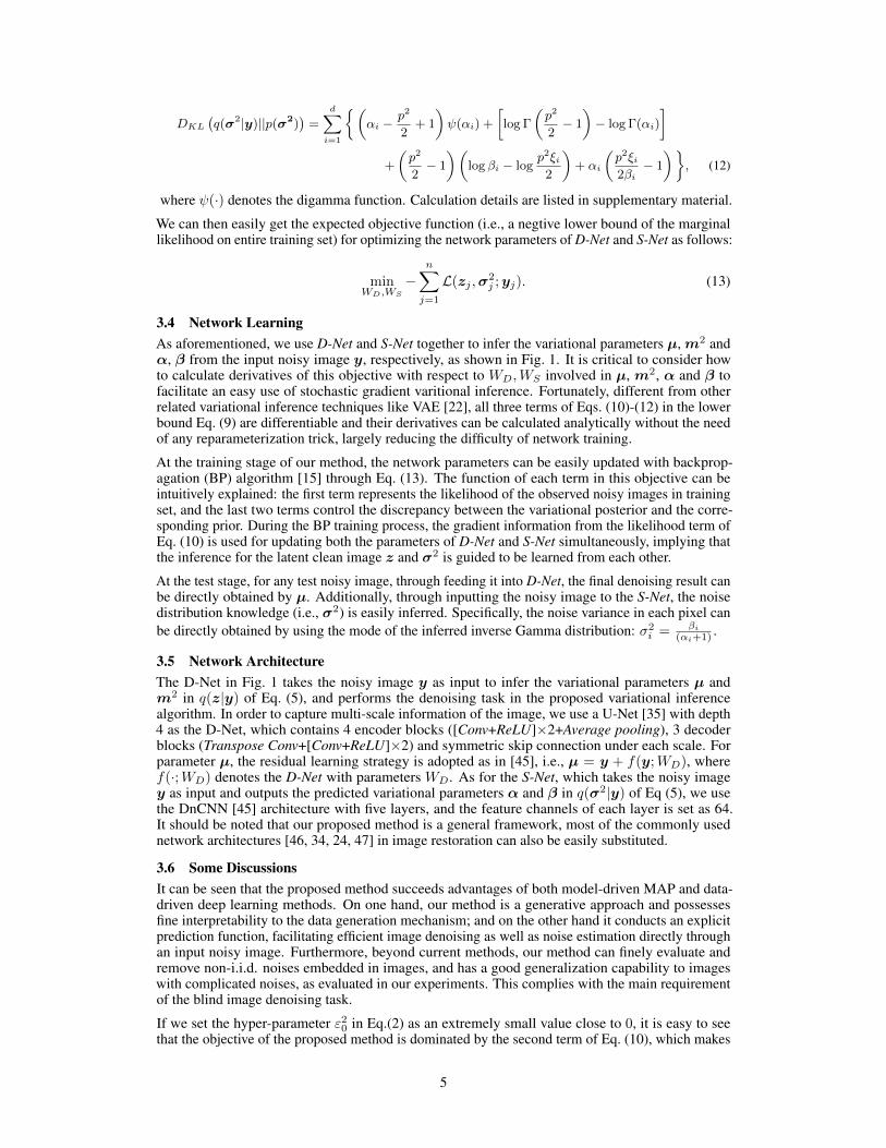
Table 1: The PSNR(dB) results of all competing methods on the three groups of test datasets. The best andsecond best results are highlighted in bold and Italic, respectively.

Cases Datasets MethodsCBM3D WNNM NCSR MLP DnCNN-B MemNet FFDNet FFDNetv UDNet VDN

Case 1Set5 27.76 26.53 26.62 27.26 29.85 30.10 30.16 30.15 28.13 30.39

LIVE1 26.58 25.27 24.96 25.71 28.81 28.96 28.99 28.96 27.19 29.22BSD68 26.51 25.13 24.96 25.58 28.73 28.74 28.78 28.77 27.13 29.02

Case 2Set5 26.34 24.61 25.76 25.73 29.04 29.55 29.60 29.56 26.01 29.80

LIVE1 25.18 23.52 24.08 24.31 28.18 28.56 28.58 28.56 25.25 28.82BSD68 25.28 23.52 24.27 24.30 28.15 28.36 28.43 28.42 25.13 28.67

Case 3Set5 27.88 26.07 26.84 26.88 29.13 29.51 29.54 29.49 27.54 29.74

LIVE1 26.50 24.67 24.96 25.26 28.17 28.37 28.39 28.38 26.48 28.65BSD68 26.44 24.60 24.95 25.10 28.11 28.20 28.22 28.20 26.44 28.46

the objective degenerate as the MSE loss generally used in traditional deep learning methods (i.e.,minimizing

∑nj=1 ||µ(yj ;WD) − xj ||2. This provides a new understanding to explain why they

incline to overfit noise bias in training data. The posterior inference process puts dominant emphasison fitting priors imposed on the latent clean image, while almost neglects the effect of noise variations.This naturally leads to its sensitiveness to unseen complicated noises contained in test images.

Very recently, both CBDNet [17] and FFDNet [46] are presented for the denoising task by feedingthe noisy image integrated with the pre-estimated noise level into the deep network to make it bettergeneralize to distinct noise types in training stage. Albeit more or less improving the generalizationcapability of network, such strategy is still too heuristic and is not easy to interpret how the inputnoise level intrinsically influence the final denoising result. Comparatively, our method is constructedin a sound Bayesian manner to estimate clean image and noise distribution together from the inputnoisy image, and its generalization can be easily explained from the perspective of generative model.

4 Experimental Results

We evaluate the performance of our method on synthetic and real datasets in this section. Allexperiments are evaluated in the sRGB space. We briefly denote our method as VDN in the following.The training and testing codes of our VDN is available at https://github.com/zsyOAOA/VDNet.

4.1 Experimental SettingNetwork training and parameter setting: The weights of D-Net and S-Net in our variationalalgorithm were initialized according to [18]. In each epoch, we randomly crop N = 64 × 5000patches with size 128× 128 from the images for training. The Adam algorithm [21] is adopted tooptimize the network parameters through minimizing the proposed negative lower bound objective.The initial learning rate is set as 2e-4 and linearly decayed in half every 10 epochs until to 1e-6. Thewindow size p in Eq. (3) is set as 7. The hyper-parameter ε20 is set as 5e-5 and 1e-6 in the followingsynthetic and real-world image denoising experiments, respectively.

Comparison methods: Several state-of-the-art denoising methods are adopted for performancecomparison, including CBM3D [11], WNNM [16], NCSR [14], MLP [10], DnCNN-B [45], Mem-Net [39], FFDNet [46], UDNet [24] and CBDNet [17]. Note that CBDNet is mainly designed forblind denoising task, and thus we only compared CBDNet on the real noise removal experiments.

6

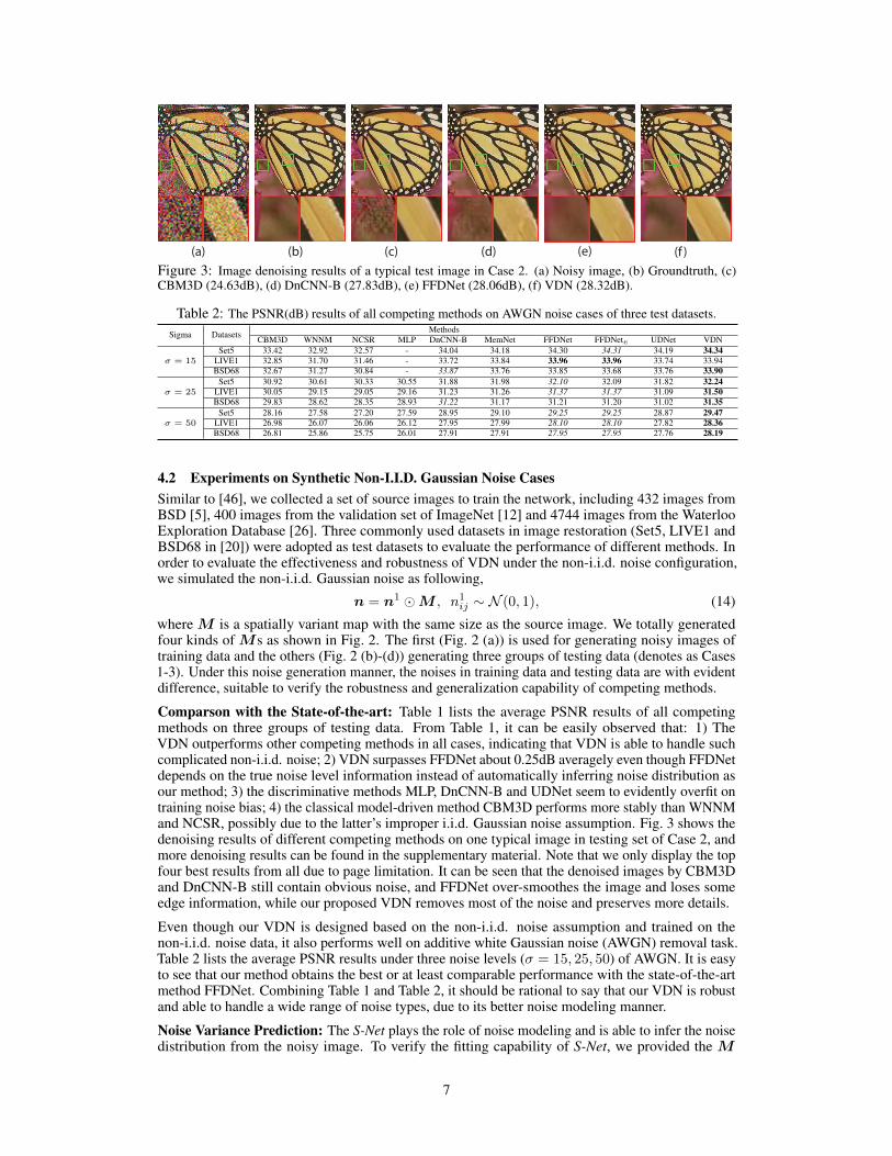
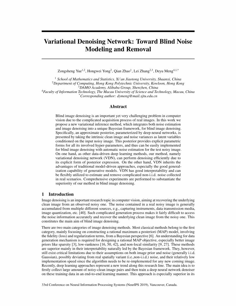
(a) (c)(b) (d) (e) (f )Figure 3: Image denoising results of a typical test image in Case 2. (a) Noisy image, (b) Groundtruth, (c)CBM3D (24.63dB), (d) DnCNN-B (27.83dB), (e) FFDNet (28.06dB), (f) VDN (28.32dB).

Table 2: The PSNR(dB) results of all competing methods on AWGN noise cases of three test datasets.Sigma Datasets Methods

CBM3D WNNM NCSR MLP DnCNN-B MemNet FFDNet FFDNete UDNet VDN

σ = 15Set5 33.42 32.92 32.57 - 34.04 34.18 34.30 34.31 34.19 34.34

LIVE1 32.85 31.70 31.46 - 33.72 33.84 33.96 33.96 33.74 33.94BSD68 32.67 31.27 30.84 - 33.87 33.76 33.85 33.68 33.76 33.90

σ = 25Set5 30.92 30.61 30.33 30.55 31.88 31.98 32.10 32.09 31.82 32.24

LIVE1 30.05 29.15 29.05 29.16 31.23 31.26 31.37 31.37 31.09 31.50BSD68 29.83 28.62 28.35 28.93 31.22 31.17 31.21 31.20 31.02 31.35

σ = 50Set5 28.16 27.58 27.20 27.59 28.95 29.10 29.25 29.25 28.87 29.47

LIVE1 26.98 26.07 26.06 26.12 27.95 27.99 28.10 28.10 27.82 28.36BSD68 26.81 25.86 25.75 26.01 27.91 27.91 27.95 27.95 27.76 28.19

4.2 Experiments on Synthetic Non-I.I.D. Gaussian Noise CasesSimilar to [46], we collected a set of source images to train the network, including 432 images fromBSD [5], 400 images from the validation set of ImageNet [12] and 4744 images from the WaterlooExploration Database [26]. Three commonly used datasets in image restoration (Set5, LIVE1 andBSD68 in [20]) were adopted as test datasets to evaluate the performance of different methods. Inorder to evaluate the effectiveness and robustness of VDN under the non-i.i.d. noise configuration,we simulated the non-i.i.d. Gaussian noise as following,

n = n1 �M , n1ij ∼ N (0, 1), (14)

where M is a spatially variant map with the same size as the source image. We totally generatedfour kinds of Ms as shown in Fig. 2. The first (Fig. 2 (a)) is used for generating noisy images oftraining data and the others (Fig. 2 (b)-(d)) generating three groups of testing data (denotes as Cases1-3). Under this noise generation manner, the noises in training data and testing data are with evidentdifference, suitable to verify the robustness and generalization capability of competing methods.

Comparson with the State-of-the-art: Table 1 lists the average PSNR results of all competingmethods on three groups of testing data. From Table 1, it can be easily observed that: 1) TheVDN outperforms other competing methods in all cases, indicating that VDN is able to handle suchcomplicated non-i.i.d. noise; 2) VDN surpasses FFDNet about 0.25dB averagely even though FFDNetdepends on the true noise level information instead of automatically inferring noise distribution asour method; 3) the discriminative methods MLP, DnCNN-B and UDNet seem to evidently overfit ontraining noise bias; 4) the classical model-driven method CBM3D performs more stably than WNNMand NCSR, possibly due to the latter’s improper i.i.d. Gaussian noise assumption. Fig. 3 shows thedenoising results of different competing methods on one typical image in testing set of Case 2, andmore denoising results can be found in the supplementary material. Note that we only display the topfour best results from all due to page limitation. It can be seen that the denoised images by CBM3Dand DnCNN-B still contain obvious noise, and FFDNet over-smoothes the image and loses someedge information, while our proposed VDN removes most of the noise and preserves more details.

Even though our VDN is designed based on the non-i.i.d. noise assumption and trained on thenon-i.i.d. noise data, it also performs well on additive white Gaussian noise (AWGN) removal task.Table 2 lists the average PSNR results under three noise levels (σ = 15, 25, 50) of AWGN. It is easyto see that our method obtains the best or at least comparable performance with the state-of-the-artmethod FFDNet. Combining Table 1 and Table 2, it should be rational to say that our VDN is robustand able to handle a wide range of noise types, due to its better noise modeling manner.

Noise Variance Prediction: The S-Net plays the role of noise modeling and is able to infer the noisedistribution from the noisy image. To verify the fitting capability of S-Net, we provided the M

7

(a) (b) (c) (d) (e) (f )

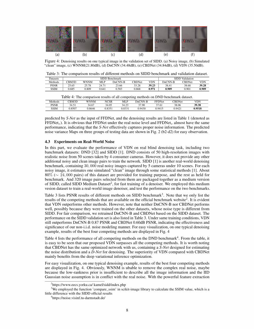
Figure 4: Denoising results on one typical image in the validation set of SIDD. (a) Noisy image, (b) Simulated“clean” image, (c) WNNM(21.80dB), (d) DnCNN (34.48dB), (e) CBDNet (34.84dB), (d) VDN (35.50dB).

Table 3: The comparison results of different methods on SIDD benchmark and validation dataset.Datasets SIDD Benchmark SIDD ValidationMethods CBM3D WNNM MLP DnCNN-B CBDNet VDN DnCNN-B CBDNet VDNPSNR 25.65 25.78 24.71 23.66 33.28 39.23 38.41 38.68 39.28SSIM 0.685 0.809 0.641 0.583 0.868 0.971 0.909 0.901 0.909

Table 4: The comparison results of all competing methods on DND benchmark dataset.Methods CBM3D WNNM NCSR MLP DnCNN-B FFDNet CBDNet VDNPSNR 34.51 34.67 34.05 34.23 37.90 37.61 38.06 39.38SSIM 0.8507 0.8646 0.8351 0.8331 0.9430 0.9415 0.9421 0.9518

predicted by S-Net as the input of FFDNet, and the denoising results are listed in Table 1 (denoted asFFDNetv). It is obvious that FFDNet under the real noise level and FFDNetv almost have the sameperformance, indicating that the S-Net effectively captures proper noise information. The predictednoise variance Maps on three groups of testing data are shown in Fig. 2 (b2-d2) for easy observation.

4.3 Experiments on Real-World NoiseIn this part, we evaluate the performance of VDN on real blind denoising task, including twobanchmark datasets: DND [32] and SIDD [1]. DND consists of 50 high-resolution images withrealistic noise from 50 scenes taken by 4 consumer cameras. However, it does not provide any otheradditional noisy and clean image pairs to train the network. SIDD [1] is another real-world denoisingbenchmark, containing 30, 000 real noisy images captured by 5 cameras under 10 scenes. For eachnoisy image, it estimates one simulated “clean” image through some statistical methods [1]. About80% (∼ 24, 000 pairs) of this dataset are provided for training purpose, and the rest as held forbenchmark. And 320 image pairs selected from them are packaged together as a medium versionof SIDD, called SIDD Medium Dataset2, for fast training of a denoiser. We employed this mediumvesion dataset to train a real-world image denoiser, and test the performance on the two benchmarks.

Table 3 lists PSNR results of different methods on SIDD benchmark3. Note that we only list theresults of the competing methods that are available on the official benchmark website2. It is evidentthat VDN outperforms other methods. However, note that neither DnCNN-B nor CBDNet performswell, possibly because they were trained on the other datasets, whose noise type is different fromSIDD. For fair comparison, we retrained DnCNN-B and CBDNet based on the SIDD dataset. Theperformance on the SIDD validation set is also listed in Table 3. Under same training conditions, VDNstill outperforms DnCNN-B 0.87 PSNR and CBDNet 0.60dB PSNR, indicating the effectiveness andsignificance of our non-i.i.d. noise modeling manner. For easy visualization, on one typical denoisingexample, results of the best four competing methods are displayed in Fig. 4

Table 4 lists the performance of all competing methods on the DND benchmark4. From the table, itis easy to be seen that our proposed VDN surpasses all the competing methods. It is worth notingthat CBDNet has the same optimized network with us, containing a S-Net designed for estimatingthe noise distribution and a D-Net for denoising. The superiority of VDN compared with CBDNetmainly benefits from the deep variational inference optimization.

For easy visualization, on one typical denoising example, results of the best four competing methodsare displayed in Fig. 4. Obviously, WNNM is ubable to remove the complex real noise, maybebecause the low-rankness prior is insufficient to describe all the image information and the IIDGaussian noise assumption is in conflict with the real noise. With the powerful feature extraction

2https://www.eecs.yorku.ca/ kamel/sidd/index.php3We employed the function ’compare_ssim’ in scikit-image library to calculate the SSIM value, which is a

little difference with the SIDD official results4https://noise.visinf.tu-darmstadt.de/

8

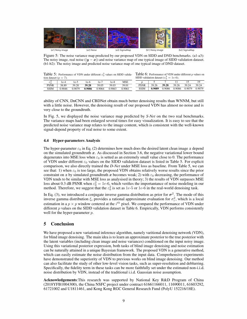
(a1) Noisy image (a2) Noise (b1) Noisy image (b2) SigmaMap(a3) SigmaMap

Figure 5: The noise variance map predicted by our proposed VDN on SIDD and DND benchmarks. (a1-a3):The noisy image, real noise (|y − x|) and noise variance map of one typical image of SIDD validation dataset.(b1-b2): The noisy image and predicted noise variance map of one typical image of DND dataset.

Table 5: Performance of VDN under different ε20 values on SIDD valida-tion dataset (p = 7).

ε20 1e-4 1e-5 1e-6 1e-7 1e-8 MSEPSNR 38.89 39.20 39.28 39.05 39.03 39.01SSIM 0.9046 0.9079 0.9086 0.9064 0.9063 0.9061

Table 6: Performance of VDN under different p values onSIDD validation dataset (ε20 = 1e-6).

p 5 7 11 15 19PSNR 39.26 39.28 39.26 39.24 39.24SSIM 0.9089 0.9086 0.9086 0.9079 0.9079

ability of CNN, DnCNN and CBDNet obtain much better denoising results than WNNM, but stillwith a little noise. However, the denoising result of our proposed VDN has almost no noise and isvery close to the groundtruth.

In Fig. 5, we displayed the noise variance map predicted by S-Net on the two real benchmarks.The variance maps had been enlarged several times for easy visualization. It is easy to see that thepredicted noise variance map relates to the image content, which is consistent with the well-knownsignal-depend property of real noise to some extent.

4.4 Hyper-parameters Analysis

The hyper-parameter ε0 in Eq. (2) determines how much does the desired latent clean image z dependon the simulated groundtruth x. As discussed in Section 3.6, the negative variational lower bounddegenerates into MSE loss when ε0 is setted as an extremely small value close to 0. The performanceof VDN under different ε0 values on the SIDD validation dataset is listed in Table 5. For explicitcomparison, we also directly trained the D-Net under MSE loss as baseline. From Table 5, we cansee that: 1) when ε0 is too large, the proposed VDN obtains relatively worse results since the priorconstraint on z by simulated groundtruth x becomes weak; 2) with ε0 decreasing, the performance ofVDN tends to be similar with MSE loss as analysised in theory; 3) the results of VDN surpasses MSEloss about 0.3 dB PSNR when ε20 = 1e-6, which verifies the importantance of noise modeling in ourmethod. Therefore, we suggest that the ε20 is set as 1e-5 or 1e-6 in the real-world denoising task.

In Eq. (3), we introduced a conjugate inverse gamma distribution as prior for σ2. The mode of thisinverse gamma distribution ξi provides a rational approximate evaluation for σ2

i , which is a localestimation in a p× p window centered at the ith pixel. We compared the performance of VDN underdifferent p values on the SIDD validation dataset in Table 6. Empirically, VDN performs consistentlywell for the hyper-parameter p.

5 Conclusion

We have proposed a new variational inference algorithm, namely varitional denoising network (VDN),for blind image denoising. The main idea is to learn an approximate posterior to the true posterior withthe latent variables (including clean image and noise variances) conditioned on the input noisy image.Using this variational posterior expression, both tasks of blind image denoising and noise estimationcan be naturally attained in a unique Bayesian framework. The proposed VDN is a generative method,which can easily estimate the noise distribution from the input data. Comprehensive experimentshave demonstrated the superiority of VDN to previous works on blind image denoising. Our methodcan also facilitate the study of other low-level vision tasks, such as super-resolution and deblurring.Specifically, the fidelity term in these tasks can be more faithfully set under the estimated non-i.i.d.noise distribution by VDN, instead of the traditional i.i.d. Gaussian noise assumption.

Acknowledgements:This research was supported by National Key R&D Program of China(2018YFB1004300), the China NSFC project under contract 61661166011, 11690011, 61603292,61721002 and U1811461, and Kong Kong RGC General Research Fund (PolyU 152216/18E).

9

References[1] Abdelrahman Abdelhamed, Stephen Lin, and Michael S. Brown. A high-quality denoising

dataset for smartphone cameras. In The IEEE Conference on Computer Vision and PatternRecognition (CVPR), June 2018.

[2] Forest Agostinelli, Michael R Anderson, and Honglak Lee. Adaptive multi-column deep neuralnetworks with application to robust image denoising. In Advances in Neural InformationProcessing Systems, pages 1493–1501, 2013.

[3] Michal Aharon, Michael Elad, Alfred Bruckstein, et al. K-svd: An algorithm for designingovercomplete dictionaries for sparse representation. IEEE Transactions on signal processing,54(11):4311, 2006.

[4] Josue Anaya and Adrian Barbu. Renoir - a dataset for real low-light noise image reduction.arXiv preprint arXiv:1409.8230, 2014.

[5] Pablo Arbelaez, Michael Maire, Charless Fowlkes, and Jitendra Malik. Contour detection andhierarchical image segmentation. IEEE Trans. Pattern Anal. Mach. Intell., 33(5):898–916, May2011.

[6] Christopher M Bishop. Pattern recognition and machine learning. springer, 2006.

[7] David M Blei, Michael I Jordan, et al. Variational inference for dirichlet process mixtures.Bayesian analysis, 1(1):121–143, 2006.

[8] Tim Brooks, Ben Mildenhall, Tianfan Xue, Jiawen Chen, Dillon Sharlet, and Jonathan T Barron.Unprocessing images for learned raw denoising. arXiv preprint arXiv:1811.11127, 2018.

[9] Antoni Buades, Bartomeu Coll, and J-M Morel. A non-local algorithm for image denoising.In 2005 IEEE Computer Society Conference on Computer Vision and Pattern Recognition(CVPR’05), volume 2, pages 60–65. IEEE, 2005.

[10] Harold C Burger, Christian J Schuler, and Stefan Harmeling. Image denoising: Can plainneural networks compete with bm3d? In 2012 IEEE conference on computer vision and patternrecognition, pages 2392–2399. IEEE, 2012.

[11] K. Dabov, A. Foi, V. Katkovnik, and K. Egiazarian. Image denoising by sparse 3-d transform-domain collaborative filtering. IEEE Transactions on Image Processing, 16(8):2080–2095, Aug2007.

[12] Jia Deng, Olga Russakovsky, Jonathan Krause, Michael Bernstein, Alexander C. Berg, andLi Fei-Fei. Scalable multi-label annotation. In ACM Conference on Human Factors in Comput-ing Systems (CHI), 2014.

[13] Weisheng Dong, Guangming Shi, and Xin Li. Nonlocal image restoration with bilateral varianceestimation: a low-rank approach. IEEE transactions on image processing, 22(2):700–711, 2013.

[14] Weisheng Dong, Lei Zhang, Guangming Shi, and Xin Li. Nonlocally centralized sparserepresentation for image restoration. IEEE transactions on Image Processing, 22(4):1620–1630,2012.

[15] Ian Goodfellow, Yoshua Bengio, and Aaron Courville. Deep learning. MIT press, 2016.

[16] Shuhang Gu, Lei Zhang, Wangmeng Zuo, and Xiangchu Feng. Weighted nuclear norm min-imization with application to image denoising. In Proceedings of the IEEE conference oncomputer vision and pattern recognition, pages 2862–2869, 2014.

[17] Shi Guo, Zifei Yan, Kai Zhang, Wangmeng Zuo, and Lei Zhang. Toward convolutional blinddenoising of real photographs. arXiv preprint arXiv:1807.04686, 2018.

[18] Kaiming He, Xiangyu Zhang, Shaoqing Ren, and Jian Sun. Delving deep into rectifiers:Surpassing human-level performance on imagenet classification. In Proceedings of the IEEEinternational conference on computer vision, pages 1026–1034, 2015.

10

[19] Viren Jain and Sebastian Seung. Natural image denoising with convolutional networks. InAdvances in neural information processing systems, pages 769–776, 2009.

[20] Jiwon Kim, Jung Kwon Lee, and Kyoung Mu Lee. Accurate image super-resolution using verydeep convolutional networks. In Proceedings of the IEEE conference on computer vision andpattern recognition, pages 1646–1654, 2016.

[21] Diederik P. Kingma and Jimmy Lei Ba. Adam: A method for stochastic optimization. interna-tional conference on learning representations, 2015.

[22] Diederik P Kingma and Max Welling. Auto-encoding variational bayes. arXiv preprintarXiv:1312.6114, 2013.

[23] Marc Lebrun, Miguel Colom, and Jean-Michel Morel. Multiscale image blind denoising. IEEETransactions on Image Processing, 24(10):3149–3161, 2015.

[24] Stamatios Lefkimmiatis. Universal denoising networks: a novel cnn architecture for imagedenoising. In Proceedings of the IEEE Conference on Computer Vision and Pattern Recognition,pages 3204–3213, 2018.

[25] Ding Liu, Bihan Wen, Yuchen Fan, Chen Change Loy, and Thomas S Huang. Non-localrecurrent network for image restoration. In Advances in Neural Information Processing Systems,pages 1673–1682, 2018.

[26] Kede Ma, Zhengfang Duanmu, Qingbo Wu, Zhou Wang, Hongwei Yong, Hongliang Li, and LeiZhang. Waterloo Exploration Database: New challenges for image quality assessment models.IEEE Transactions on Image Processing, 26(2):1004–1016, Feb. 2017.

[27] Matteo Maggioni, Vladimir Katkovnik, Karen Egiazarian, and Alessandro Foi. Nonlocaltransform-domain filter for volumetric data denoising and reconstruction. IEEE transactions onimage processing, 22(1):119–133, 2013.

[28] Julien Mairal, Michael Elad, and Guillermo Sapiro. Sparse representation for color imagerestoration. IEEE Transactions on image processing, 17(1):53–69, 2008.

[29] Xiaojiao Mao, Chunhua Shen, and Yu-Bin Yang. Image restoration using very deep convo-lutional encoder-decoder networks with symmetric skip connections. In Advances in neuralinformation processing systems, pages 2802–2810, 2016.

[30] Deyu Meng and Fernando De La Torre. Robust matrix factorization with unknown noise. InIEEE International Conference on Computer Vision, 2013.

[31] Pietro Perona and Jitendra Malik. Scale-space and edge detection using anisotropic diffusion.IEEE Transactions on pattern analysis and machine intelligence, 12(7):629–639, 1990.

[32] Tobias Plotz and Stefan Roth. Benchmarking denoising algorithms with real photographs.In Proceedings of the IEEE Conference on Computer Vision and Pattern Recognition, pages1586–1595, 2017.

[33] Tobias Plötz and Stefan Roth. Neural nearest neighbors networks. In Advances in NeuralInformation Processing Systems, pages 1087–1098, 2018.

[34] Tobias Plötz and Stefan Roth. Neural nearest neighbors networks. In S. Bengio, H. Wallach,H. Larochelle, K. Grauman, N. Cesa-Bianchi, and R. Garnett, editors, Advances in NeuralInformation Processing Systems 31, pages 1087–1098. Curran Associates, Inc., 2018.

[35] Olaf Ronneberger, Philipp Fischer, and Thomas Brox. U-net: Convolutional networks forbiomedical image segmentation. In International Conference on Medical image computing andcomputer-assisted intervention, pages 234–241. Springer, 2015.

[36] Stefan Roth and Michael J Black. Fields of experts. International Journal of Computer Vision,82(2):205, 2009.

[37] Leonid I Rudin, Stanley Osher, and Emad Fatemi. Nonlinear total variation based noise removalalgorithms. Physica D: nonlinear phenomena, 60(1-4):259–268, 1992.

11

[38] Eero P Simoncelli and Edward H Adelson. Noise removal via bayesian wavelet coring. InProceedings of 3rd IEEE International Conference on Image Processing, volume 1, pages379–382. IEEE, 1996.

[39] Ying Tai, Jian Yang, Xiaoming Liu, and Chunyan Xu. Memnet: A persistent memory networkfor image restoration. In Proceedings of the IEEE international conference on computer vision,pages 4539–4547, 2017.

[40] Yanghai Tsin, Visvanathan Ramesh, and Takeo Kanade. Statistical calibration of ccd imagingprocess. In Proceedings Eighth IEEE International Conference on Computer Vision. ICCV2001, volume 1, pages 480–487. IEEE, 2001.

[41] Junyuan Xie, Linli Xu, and Enhong Chen. Image denoising and inpainting with deep neuralnetworks. In Advances in neural information processing systems, pages 341–349, 2012.

[42] Jun Xu, Lei Zhang, and David Zhang. A trilateral weighted sparse coding scheme for real-worldimage denoising. In The European Conference on Computer Vision (ECCV), September 2018.

[43] Hongwei Yong, Deyu Meng, Wangmeng Zuo, and Lei Zhang. Robust online matrix factorizationfor dynamic background subtraction. IEEE transactions on pattern analysis and machineintelligence, 40(7):1726–1740, 2017.

[44] Zongsheng Yue, Deyu Meng, Yongqing Sun, and Qian Zhao. Hyperspectral image restorationunder complex multi-band noises. Remote Sensing, 10(10):1631, 2018.

[45] Kai Zhang, Wangmeng Zuo, Yunjin Chen, Deyu Meng, and Lei Zhang. Beyond a gaussiandenoiser: Residual learning of deep cnn for image denoising. IEEE Transactions on ImageProcessing, 26(7):3142–3155, 2017.

[46] Kai Zhang, Wangmeng Zuo, and Lei Zhang. Ffdnet: Toward a fast and flexible solution forcnn-based image denoising. IEEE Transactions on Image Processing, 27(9):4608–4622, 2018.

[47] Yulun Zhang, Yapeng Tian, Yu Kong, Bineng Zhong, and Yun Fu. Residual dense networkfor image super-resolution. In Proceedings of the IEEE Conference on Computer Vision andPattern Recognition, pages 2472–2481, 2018.

[48] Qian Zhao, Deyu Meng, Zongben Xu, Wangmeng Zuo, and Lei Zhang. Robust principalcomponent analysis with complex noise. In Proceedings of The 31st International Conferenceon Machine Learning, pages 55–63, 2014.

[49] Fengyuan Zhu, Guangyong Chen, Jianye Hao, and Pheng-Ann Heng. Blind image denoisingvia dependent dirichlet process tree. IEEE transactions on pattern analysis and machineintelligence, 39(8):1518–1531, 2017.

[50] Fengyuan Zhu, Guangyong Chen, and Pheng-Ann Heng. From noise modeling to blind imagedenoising. In Proceedings of the IEEE Conference on Computer Vision and Pattern Recognition,pages 420–429, 2016.

12