Embed Size (px)
Citation preview
Variational Inference for GPs: Presenters
Group1: Stochastic variational inference. Slides 2 - 28
Chaoqi Wang
Sana Tonekaboni
Will Grathwohl
Group2: Variational inference for GPs. Slides 29 - 57
Trefor Evans
Kingsley Chang
Shems Saleh
James Lucas
Group3: PAC-Bayes. Slides 58 - 68
Wenyuan Zeng
Shengyang Sun
Variational Inference for GPs October 17, 2017 1 / 68
Variational Inference for GPsCSC2541 Presentation
October 17, 2017
Variational Inference for GPs October 17, 2017 2 / 68
Stochastic Variational Inference,by Matt Hoffman, David M. Blei, Chong Wang, John
Paisley
Exponential family and Latent Dirichlet Allocation
Variational Inference for GPs October 17, 2017 3 / 68
Exponential family
Exponential family plays a very important role in statistics and it has manygood properties.
1 Most of the commonly used distributions are in the exponential family,like, Gaussian, multinomial, exponential, Dirichlet, Poisson, Gamma...
2 Also, some are not in the exponential family: Cauchy, uniform...
Variational Inference for GPs October 17, 2017 4 / 68
Exponential family: definition
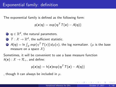
The exponential family is defined as the following form:
p(x |η) = exp{ηTT (x)− A(η)}
1 η ∈ Rd , the natural parameters.
2 T : X → Rd , the sufficient statistic.
3 A(η) = ln∫X exp{ηTT (x)}dµ(x), the log normalizer. (µ is the base
measure on a space X )
Sometimes, it will be convenient to use a base measure functionh(x) : X → R+, and define:
p(x|η) = h(x)exp{ηTT (x)− A(η)}
, though h can always be included in µ.
Variational Inference for GPs October 17, 2017 5 / 68
Exponential family: examples
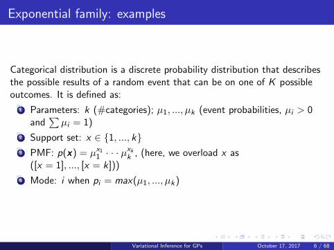
Categorical distribution is a discrete probability distribution that describesthe possible results of a random event that can be on one of K possibleoutcomes. It is defined as:
1 Parameters: k (#categories); µ1, ..., µk (event probabilities, µi > 0and
∑µi = 1)
2 Support set: x ∈ {1, ..., k}3 PMF: p(x) = µx1
1 · · · µxkk , (here, we overload x as
([x = 1], ..., [x = k]))
4 Mode: i when pi = max(µ1, ..., µk )
Variational Inference for GPs October 17, 2017 6 / 68
Exponential family: examples
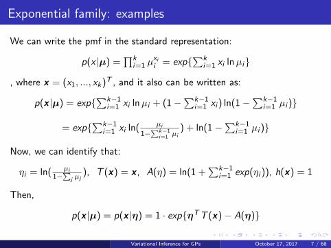
We can write the pmf in the standard representation:
p(x |µ) =∏k
i=1 µxii = exp{∑k
i=1 xi lnµi}
, where x = (x1, ..., xk )T , and it also can be written as:
p(x |µ) = exp{∑k−1i=1 xi lnµi + (1−∑k−1
i=1 xi ) ln(1−∑k−1i=1 µi )}
= exp{∑k−1i=1 xi ln( µi
1−∑k−1i=1 µi
) + ln(1−∑k−1i=1 µi )}
Now, we can identify that:
ηi = ln( µi1−∑j µj
), T (x) = x , A(η) = ln(1 +∑k−1
i=1 exp(ηi )), h(x) = 1
Then,
p(x |µ) = p(x |η) = 1 · exp{ηTT (x)− A(η)}
Variational Inference for GPs October 17, 2017 7 / 68
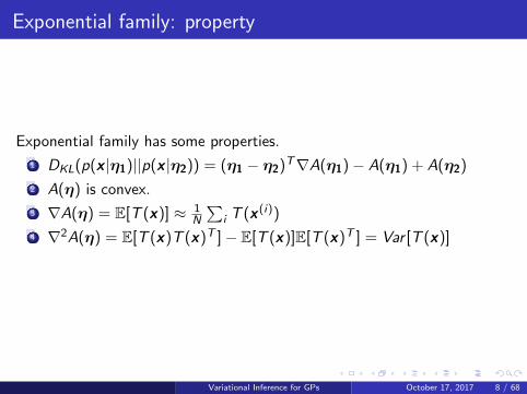
Exponential family: property
Exponential family has some properties.
1 DKL(p(x |η1)||p(x |η2)) = (η1 − η2)T∇A(η1)− A(η1) + A(η2)
2 A(η) is convex.
3 ∇A(η) = E[T (x)] ≈ 1N
∑i T (x (i))
4 ∇2A(η) = E[T (x)T (x)T ]− E[T (x)]E[T (x)T ] = Var [T (x)]
Variational Inference for GPs October 17, 2017 8 / 68
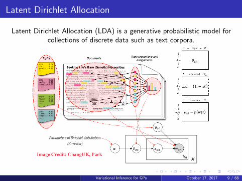
Latent Dirichlet Allocation
Latent Dirichlet Allocation (LDA) is a generative probabilistic model forcollections of discrete data such as text corpora.
Variational Inference for GPs October 17, 2017 9 / 68
LDA: process
The generative process of LDA model can be summarized as:
1 Draw topics βk from Dirichlet(η, ..., η) for k ∈ {1, ...,K}2 For each document d ∈ {1, ...,D} :
1 Draw topic proportions θd from Dirichlet(α, ..., α)2 For each word w ∈ {1, ...,N} :
Draw topic assignment zdn from Multinomial(θd )Draw word wdn from Multinomial(βzdn )
Variational Inference for GPs October 17, 2017 10 / 68

Latent Dirichlet Allocation: notations
There are some notations used in LDA model:
1 wdn is the nth word in dth document. Each word is an element in thefixed vocabulary of V terms.
2 βk is a V dimensional vector, on a V − 1 simplex. The w th entry intopic k is βkw
3 θd is the associated topic proportions of dth document. It is a pointon the K − 1 simplex.
4 zdn indexes the topic from which wdn is drawn. It is assumed thateach word in each document is drawn from a single topic.
Variational Inference for GPs October 17, 2017 11 / 68
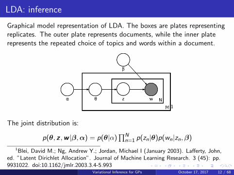
LDA: inference
Graphical model representation of LDA. The boxes are plates representingreplicates. The outer plate represents documents, while the inner platerepresents the repeated choice of topics and words within a document.
1
The joint distribution is:
p(θ, z ,w |β,α) = p(θ|α)∏N
n=1 p(zn|θ)p(wn|zn,β)
1Blei, David M.; Ng, Andrew Y.; Jordan, Michael I (January 2003). Lafferty, John,ed. ”Latent Dirichlet Allocation”. Journal of Machine Learning Research. 3 (45): pp.9931022. doi:10.1162/jmlr.2003.3.4-5.993
Variational Inference for GPs October 17, 2017 12 / 68
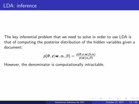
LDA: inference
The key inferential problem that we need to solve in order to use LDA isthat of computing the posterior distribution of the hidden variables given adocument:
p(θ, z |w ,α,β) = p(θ,z ,w |β,α)p(w |α,β)
However, the denominator is computationally intractable.
Variational Inference for GPs October 17, 2017 13 / 68
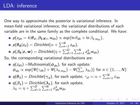
LDA: inference
One way to approximate the posterior is variational inference. Inmean-field variational inference, the variational distributions of eachvariable are in the same family as the complete conditional. We have:
p(zdn = k |θd ,β1:K ,,wdn) ∝ exp{ln θdk + lnβk,wdn},
p(θd |zd ) = Dirichlet(α +∑N
n=1 zdn),
p(βk |z,w) = Dirichlet(η +∑D
d=1
∑Nn=1 z
kdnwdn)
So, the corresponding variational distributions are:
q(zdn) =Multinomial(φdn), for each update:φdn ∝ exp{Ψ(γdk ) + Ψ(λk,wdn
)−Ψ(∑
v λkv )} for n ∈ {1, ...,N}q(θd ) = Dirichlet(γd ), for each update, γd = α +
∑Nn=1 φdn
q(βk ) = Dirichlet(λk ), for each update,λk = η +
∑Dd=1
∑Nn=1 φ
kdnwdn
Variational Inference for GPs October 17, 2017 14 / 68

LDA: inference
Before updating the topics λ1:K , we need to compute the local variationalparameters for every document. This is particularly wasteful in thebeginning of the algorithm when, before completing the first iteration, wemust analyze every document with randomly initialized topics.
Variational Inference for GPs October 17, 2017 15 / 68
Stochastic Variational Inference,by Matt Hoffman, David M. Blei, Chong Wang, John
Paisley
Variational Inference
Variational Inference for GPs October 17, 2017 16 / 68
Variational Inference
Goal: approximate the posterior distribution of a probabilistic modelby introducing a distribution over the hidden variables, and optimizingthe parameters of that distribution.
Our class of models involves:
Obsevations x = x1:N
Global hidden variables β
Local hidden variables z = z1:N
Fixed parameters α (For simplicity we assume that they only governthe global hidden variables)
Variational Inference for GPs October 17, 2017 17 / 68
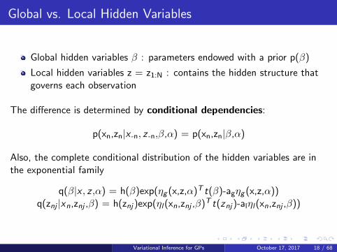
Global vs. Local Hidden Variables
Global hidden variables β : parameters endowed with a prior p(β)
Local hidden variables z = z1:N : contains the hidden structure thatgoverns each observation
The difference is determined by conditional dependencies:
p(xn,zn|x -n, z -n,β,α) = p(xn,zn|β,α)
Also, the complete conditional distribution of the hidden variables are inthe exponential family
q(β|x , z ,α) = h(β)exp(ηg (x,z,α)T t(β)-agηg (x,z,α))q(znj |xn,znj ,β) = h(znj )exp(ηl (xn,znj ,β)T t(znj )-alηl (xn,znj ,β))
Variational Inference for GPs October 17, 2017 18 / 68
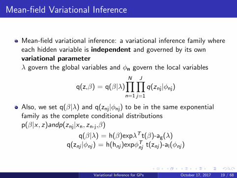
Mean-field Variational Inference
Mean-field variational inference: a variational inference family whereeach hidden variable is independent and governed by its ownvariational parameterλ govern the global variables and φn govern the local variables
q(z,β) = q(β|λ)N∏
n=1
J∏
j=1
q(znj|φnj)
Also, we set q(β|λ) and q(znj|φnj) to be in the same exponentialfamily as the complete conditional distributionsp(β|x , z)andp(znj|xn, zn-j,β)
q(β|λ) = h(β)expλT t(β)-ag(λ)q(znj |φnj ) = h(hnj )expφT
nj t(znj )-al(φnj )
Variational Inference for GPs October 17, 2017 19 / 68
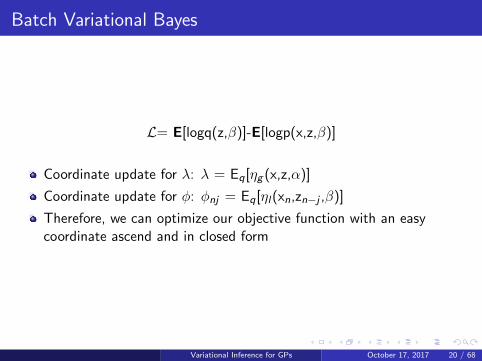
Batch Variational Bayes
L= E[logq(z,β)]-E[logp(x,z,β)]
Coordinate update for λ: λ = Eq[ηg (x,z,α)]
Coordinate update for φ: φnj = Eq[ηl (xn,zn−j ,β)]
Therefore, we can optimize our objective function with an easycoordinate ascend and in closed form
Variational Inference for GPs October 17, 2017 20 / 68
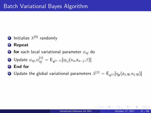
Batch Variational Bayes Algorithm
1 Initialize λ(0) randomly
2 Repeat
3 for each local variational parameter φnj do
4 Update φnj ,φ(t)nj = Eq(t−1) [ηl ,j (xn,zn−j ,β)]
5 End for
6 Update the global variational parameters λ(t) = Eq(t) [ηg (z1:N ,x1:N)]
Variational Inference for GPs October 17, 2017 21 / 68
Stochastic Variational Inference
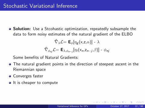
Solution: Use a Stcohastic optimization, repeatedly subsample thedata to form noisy estimates of the natural gradient of the ELBO
∇λL= Eφ[ηg (x,z,α)] - λ
∇φnjL= Eλ,φn−j
[ηl (xn,zn−j ,β)] - φnj
Some benefits of Natural Gradients:
The natural gradient points in the direction of steepest ascent in theRiemannian space
Converges faster
It is cheaper to compute
Variational Inference for GPs October 17, 2017 22 / 68
Stochastic Variational Inference Algorithm
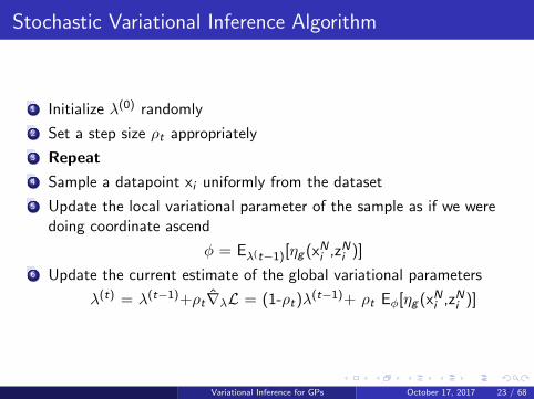
1 Initialize λ(0) randomly
2 Set a step size ρt appropriately
3 Repeat
4 Sample a datapoint xi uniformly from the dataset
5 Update the local variational parameter of the sample as if we weredoing coordinate ascend
φ = Eλ(t−1)[ηg (xNi ,zN
i )]
6 Update the current estimate of the global variational parameters
λ(t) = λ(t−1)+ρt∇λL = (1-ρt)λ(t−1)+ ρt Eφ[ηg (xNi ,zN
i )]
Variational Inference for GPs October 17, 2017 23 / 68
A Review Of Stochastic Gradient Variational Bayes
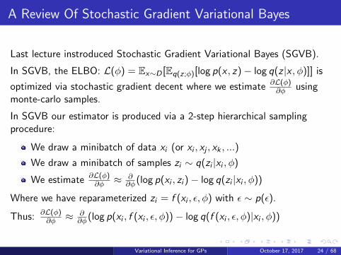
Last lecture instroduced Stochastic Gradient Variational Bayes (SGVB).
In SGVB, the ELBO: L(φ) = Ex∼D [Eq(z;φ)[log p(x , z)− log q(z |x , φ)]] is
optimized via stochastic gradient decent where we estimate ∂L(φ)∂φ using
monte-carlo samples.
In SGVB our estimator is produced via a 2-step hierarchical samplingprocedure:
We draw a minibatch of data xi (or xi , xj , xk , ...)
We draw a minibatch of samples zi ∼ q(zi |xi , φ)
We estimate ∂L(φ)∂φ ≈ ∂
∂φ(log p(xi , zi )− log q(zi |xi , φ))
Where we have reparameterized zi = f (xi , ε, φ) with ε ∼ p(ε).
Thus: ∂L(φ)∂φ ≈ ∂
∂φ(log p(xi , f (xi , ε, φ))− log q(f (xi , ε, φ)|xi , φ))
Variational Inference for GPs October 17, 2017 24 / 68
Required Properties
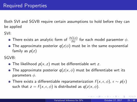
Both SVI and SGVB require certain assumptions to hold before they canbe applied
SVI:
There exists an analytic form of ∂L(φ)∂φ for each model paraemter φ.
The approximate posterior q(z |φ) must be in the same exponentialfamily as p(z)
SGVB:
The likelihood p(x , z) must be differentiable wrt z .
The approximate posterior q(z |x , φ) must be differentiabe wrt itsparameters φ.
There exists a differentiable reparameterization f (x , ε, φ), ε ∼ p(ε)such that z = f (x , ε, φ) is distributed as q(z |x , φ).
Variational Inference for GPs October 17, 2017 25 / 68
SVI
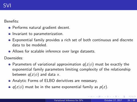
Benefits:
Performs natural gradient decent.
Invariant to parameterization.
Exponential family provides a rich set of both continuous and discretedata to be modeled.
Allows for scalable inference over large datasets.
Downsides:
Parameters of variational approximation q(z |φ) must be exactly theexponential family parameters limiting complexity of the relationshipbetween q(z |φ) and data x .
Analytic Forms of ELBO derivitives are nessesary.
q(z |φ) must be in the same exponential family as p(z).
Variational Inference for GPs October 17, 2017 26 / 68
SGVB
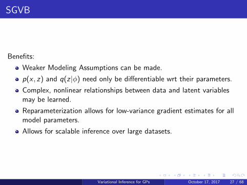
Benefits:
Weaker Modeling Assumptions can be made.
p(x , z) and q(z |φ) need only be differentiable wrt their parameters.
Complex, nonlinear relationships between data and latent variablesmay be learned.
Reparameterization allows for low-variance gradient estimates for allmodel parameters.
Allows for scalable inference over large datasets.
Variational Inference for GPs October 17, 2017 27 / 68
SGVB Continued
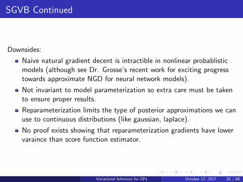
Downsides:
Naive natural gradient decent is intractible in nonlinear probablisticmodels (although see Dr. Grosse’s recent work for exciting progresstowards approximate NGD for neural network models).
Not invariant to model parameterization so extra care must be takento ensure proper results.
Reparameterization limits the type of posterior approximations we canuse to continuous distributions (like gaussian, laplace).
No proof exists showing that reparameterization gradients have lowervaraince than score function estimator.
Variational Inference for GPs October 17, 2017 28 / 68
Variational Inference for GPs
Sparse Gaussian Process
Variational Inference for GPs October 17, 2017 29 / 68
Gaussian Processes Review
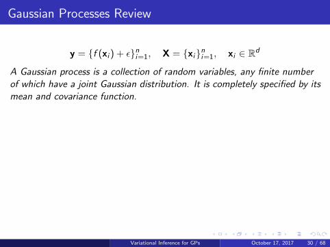
y = {f (xi ) + ε}ni=1, X = {xi}n
i=1, xi ∈ Rd
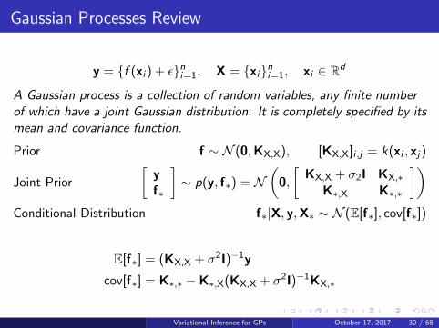
A Gaussian process is a collection of random variables, any finite numberof which have a joint Gaussian distribution. It is completely specified by itsmean and covariance function.
Prior f ∼ N (0,KX,X), [KX,X]i ,j = k(xi , xj )
Joint Prior
[yf∗
]∼ p(y, f∗) = N
(0,
[KX,X + σ2I KX,∗
K∗,X K∗,∗
])
Conditional Distribution f∗|X, y,X∗ ∼ N (E[f∗], cov[f∗])
E[f∗] = (KX,X + σ2I)−1y
cov[f∗] = K∗,∗ −K∗,X(KX,X + σ2I)−1KX,∗
Variational Inference for GPs October 17, 2017 30 / 68
Gaussian Processes Review
y = {f (xi ) + ε}ni=1, X = {xi}n
i=1, xi ∈ Rd
A Gaussian process is a collection of random variables, any finite numberof which have a joint Gaussian distribution. It is completely specified by itsmean and covariance function.
Prior f ∼ N (0,KX,X), [KX,X]i ,j = k(xi , xj )
Joint Prior
[yf∗
]∼ p(y, f∗) = N
(0,
[KX,X + σ2I KX,∗
K∗,X K∗,∗
])
Conditional Distribution f∗|X, y,X∗ ∼ N (E[f∗], cov[f∗])
E[f∗] = (KX,X + σ2I)−1y
cov[f∗] = K∗,∗ −K∗,X(KX,X + σ2I)−1KX,∗
Variational Inference for GPs October 17, 2017 30 / 68
Model Selection
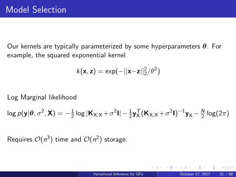
Our kernels are typically parameterized by some hyperparameters θ. Forexample, the squared exponential kernel
k(x, z) = exp(−||x−z||22/θ2)
Log Marginal likelihood
log p(y|θ, σ2,X) = −12 log |KX,X+σ2I|− 1
2yTX (KX,X+σ2I)−1yX− N
2 log(2π)
Requires O(n3) time and O(n2) storage.
Variational Inference for GPs October 17, 2017 31 / 68
Modifying the Joint Prior
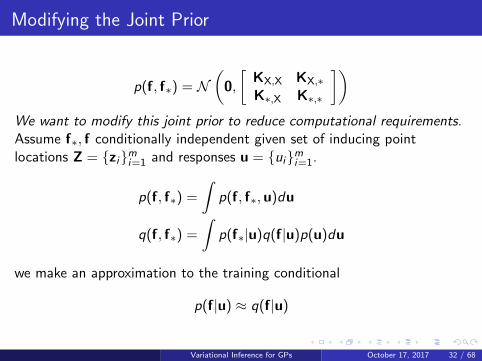
p(f, f∗) = N(
0,
[KX,X KX,∗K∗,X K∗,∗
])
We want to modify this joint prior to reduce computational requirements.Assume f∗, f conditionally independent given set of inducing pointlocations Z = {zi}m
i=1 and responses u = {ui}mi=1.
p(f, f∗) =
∫p(f, f∗,u)du
q(f, f∗) =
∫p(f∗|u)q(f|u)p(u)du
we make an approximation to the training conditional
p(f|u) ≈ q(f|u)
Variational Inference for GPs October 17, 2017 32 / 68
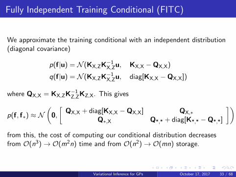
Fully Independent Training Conditional (FITC)
We approximate the training conditional with an independent distribution(diagonal covariance)
p(f|u) = N (KX,ZK−1X,Zu, KX,X −QX,X)
q(f|u) = N (KX,ZK−1X,Zu, diag[KX,X −QX,X])
where QX,X = KX,ZK−1Z,ZKZ,X. This gives
p(f, f∗) ≈ N(
0,
[QX,X + diag[KX,X −QX,X] QX,∗
Q∗,X Q*,* + diag[K*,* −Q*,*]
])
from this, the cost of computing our conditional distribution decreasesfrom O(n3)→ O(m2n) time and from O(n2)→ O(mn) storage.
Variational Inference for GPs October 17, 2017 33 / 68
Variational Inference for GPs
Adapted from a presentation by ”Variational Model Selection for SparseGaussian Process Regression” Christopher. P. Ley (2016) 2
2http://games.cmm.uchile.cl/media/uploads/posts/SGP_presentation.pdf
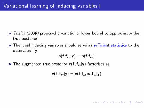
Variational learning of inducing variables I
Titsias (2009) proposed a variational lower bound to approximate thetrue posterior.
The ideal inducing variables should serve as sufficient statistics to theobservation y.
p(f|fm, y) = p(f|fm)
The augmented true posterior p(f, fm|y) factorises as
p(f, fm|y) = p(f|fm)p(fm|y)
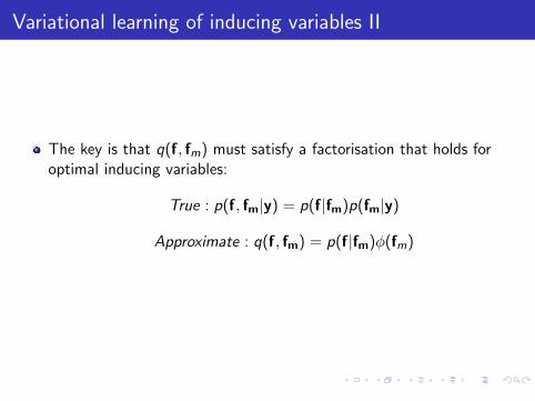
Variational learning of inducing variables II
The key is that q(f, fm) must satisfy a factorisation that holds foroptimal inducing variables:
True : p(f, fm|y) = p(f|fm)p(fm|y)
Approximate : q(f, fm) = p(f|fm)φ(fm)
Variational Model Selection for Sparse Gaussian Process Regression
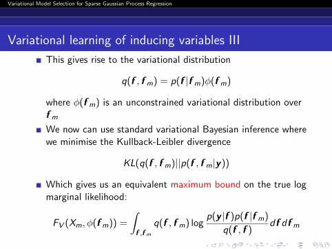
Variational learning of inducing variables III
This gives rise to the variational distribution
q(f , f m) = p(f |f m)φ(f m)
where φ(f m) is an unconstrained variational distribution overf m
We now can use standard variational Bayesian inference wherewe minimise the Kullback-Leibler divergence
KL(q(f , f m)||p(f , f m|y))
Which gives us an equivalent maximum bound on the true logmarginal likelihood:
FV (Xm, φ(f m)) =
∫
f ,f m
q(f , f m) logp(y |f )p(f |f m)
q(f , f )df df m
Variational Model Selection for Sparse Gaussian Process Regression
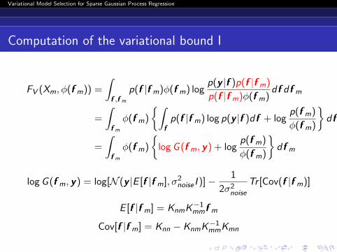
Computation of the variational bound I
FV (Xm, φ(f m)) =
∫
f ,f m
p(f |f m)φ(f m) logp(y |f )p(f |f m)
p(f |f m)φ(f m)df df m
=
∫
f m
φ(f m)
{∫
fp(f |f m) log p(y |f )df + log
p(f m)
φ(f m)
}df m
=
∫
f m
φ(f m)
{logG (f m, y) + log
p(f m)
φ(f m)
}df m
logG (f m, y) = log[N (y |E [f |f m], σ2noise I )]− 1
2σ2noise
Tr [Cov(f |f m)]
E [f |f m] = KnmK−1mmf m
Cov[f |f m] = Knn − KnmK−1mmKmn
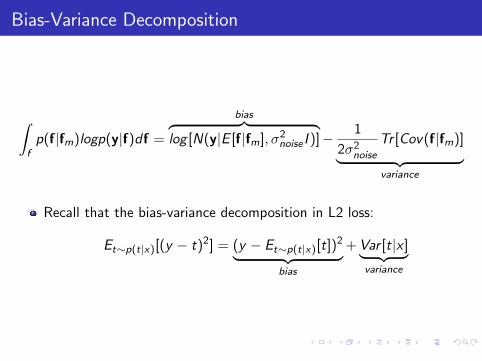
Bias-Variance Decomposition
∫
fp(f|fm)logp(y|f)df =
bias︷ ︸︸ ︷log [N(y|E [f|fm], σ2noise I )]− 1
2σ2noise
Tr [Cov(f|fm)]
︸ ︷︷ ︸variance
Recall that the bias-variance decomposition in L2 loss:
Et∼p(t|x)[(y − t)2] = (y − Et∼p(t|x)[t])2︸ ︷︷ ︸
bias
+Var [t|x ]︸ ︷︷ ︸variance
Variational Model Selection for Sparse Gaussian Process Regression
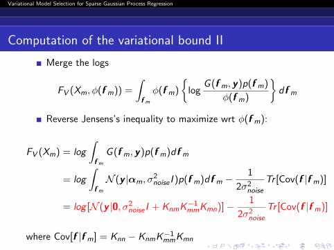
Computation of the variational bound II
Merge the logs
FV (Xm, φ(f m)) =
∫
f m
φ(f m)
{log
G (f m, y)p(f m)
φ(f m)
}df m
Reverse Jensens’s inequality to maximize wrt φ(f m):
FV (Xm) = log
∫
f m
G (f m, y)p(f m)df m
= log
∫
f m
N (y |αm, σ2noise I )p(f m)df m −
1
2σ2noise
Tr [Cov(f |f m)]
= log [N (y |0, σ2noise I + KnmK
−1mmKmn)]− 1
2σ2noise
Tr [Cov(f |f m)]
where Cov[f |f m] = Knn − KnmK−1mmKmn
Variational Model Selection for Sparse Gaussian Process Regression
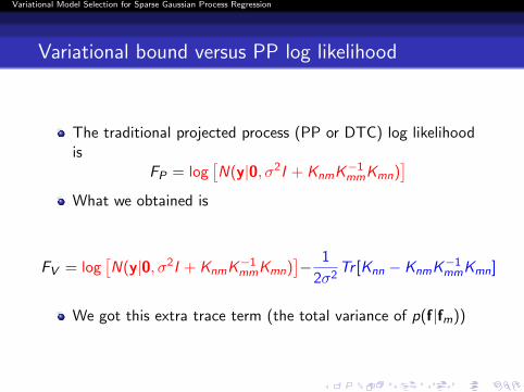
Variational bound versus PP log likelihood
The traditional projected process (PP or DTC) log likelihoodis
FP = log[N(y|0, σ2I + KnmK
−1mmKmn)
]
What we obtained is
FV = log[N(y|0, σ2I + KnmK
−1mmKmn)
]− 1
2σ2Tr [Knn − KnmK
−1mmKmn]
We got this extra trace term (the total variance of p(f|fm))
Variational Model Selection for Sparse Gaussian Process Regression
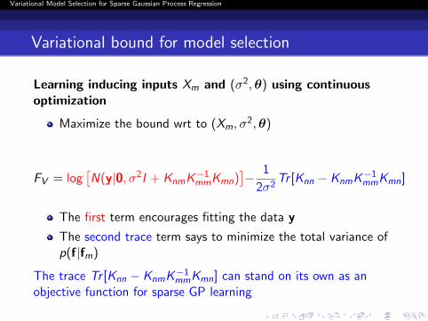
Variational bound for model selection
Learning inducing inputs Xm and (σ2,θ) using continuousoptimization
Maximize the bound wrt to (Xm, σ2,θ)
FV = log[N(y|0, σ2I + KnmK
−1mmKmn)
]− 1
2σ2Tr [Knn − KnmK
−1mmKmn]
The first term encourages fitting the data y
The second trace term says to minimize the total variance ofp(f|fm)
The trace Tr [Knn − KnmK−1mmKmn] can stand on its own as an
objective function for sparse GP learning
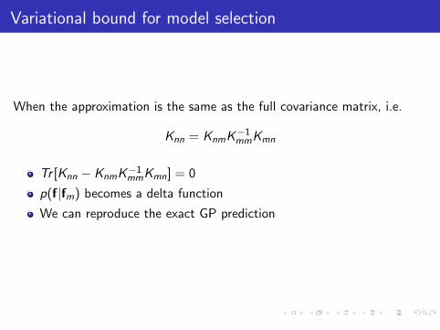
Variational bound for model selection
When the approximation is the same as the full covariance matrix, i.e.
Knn = KnmK−1mmKmn
Tr [Knn − KnmK−1mmKmn] = 0
p(f|fm) becomes a delta function
We can reproduce the exact GP prediction
Variational Model Selection for Sparse Gaussian Process Regression
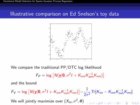
Illustrative comparison on Ed Snelson’s toy data
0 1 2 3 4 5 6−2
−1.5
−1
−0.5
0
0.5
1
1.5
2
We compare the traditional PP/DTC log likelihood
FP = log[N(y|0, σ2I + KnmK
−1mmKmn)
]
and the bound
FV = log[N(y|0, σ2I + KnmK
−1mmKmn)
]− 1
2σ2Tr [Knn − KnmK
−1mmKmn]
We will jointly maximize over (Xm, σ2,θ)
Variational Model Selection for Sparse Gaussian Process Regression
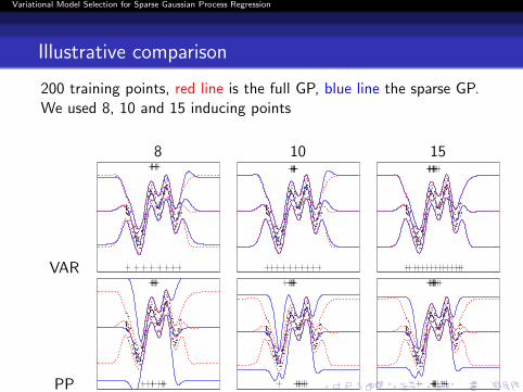
Illustrative comparison
200 training points, red line is the full GP, blue line the sparse GP.We used 8, 10 and 15 inducing points
8 10 15
VAR
PP
Variational bound compared to PP likelihood
The variational method (VFE) converges to the full GP model as weincrease the number of inducing variables. But PP would not.
VFE tends to find smoother distribution than the fill GP when theinducing vairaibles are not enough.
PP tends to interpolate the training examples.
Variational Inference for GPs
FITC and VFE Comparison
Variational Inference for GPs October 17, 2017 40 / 68

Overview of the two methods
Negative Log Marginal Likelihood:
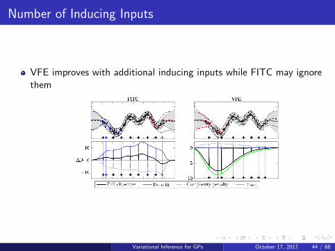
Data fit: Penalizes data outside the covariance ellipse Qff + GComplexity penalty: Characterizes the volume of possible datasetscompatible with the data fit term. (Occam’s Razor)Trace term: Ensure that objective function is a true lower bound tomarginal likelihood of the full GP
Variational Inference for GPs October 17, 2017 41 / 68
Overview
Points of comparison:
1 Noise Variance
2 Number of Inducing Inputs
3 True GP Posterior
4 Optimas
Variational Inference for GPs October 17, 2017 42 / 68
Noise Variance
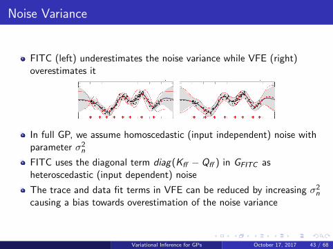
FITC (left) underestimates the noise variance while VFE (right)overestimates it
In full GP, we assume homoscedastic (input independent) noise withparameter σ2n
FITC uses the diagonal term diag(Kff − Qff ) in GFITC asheteroscedastic (input dependent) noise
The trace and data fit terms in VFE can be reduced by increasing σ2ncausing a bias towards overestimation of the noise variance
Variational Inference for GPs October 17, 2017 43 / 68
Number of Inducing Inputs
VFE improves with additional inducing inputs while FITC may ignorethem
Variational Inference for GPs October 17, 2017 44 / 68
Number of Inducing Inputs
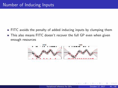
FITC avoids the penalty of added inducing inputs by clumping them
This also means FITC doesn’t recover the full GP even when givenenough resources
Variational Inference for GPs October 17, 2017 45 / 68
Local Optima
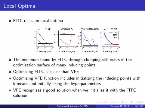
FITC relies on local optima
The minimum found by FITC through clumping still exists in theoptimization surface of many inducing points
Optimizing FITC is easier than VFE
Optimizing VFE function includes initializing the inducing points withk-means and initially fixing the hyperparameters
VFE recognizes a good solution when we initialize it with the FITCsolution
Variational Inference for GPs October 17, 2017 46 / 68
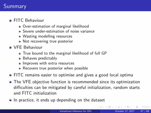
Summary
FITC Behaviour
Over-estimation of marginal likelihoodSevere under-estimation of noise varianceWasting modelling resourcesNot recovering true posterior
VFE Behaviour
True bound to the marginal likelihood of full GPBehaves predictablyImproves with extra resourcesRecovers true posterior when possible
FITC remains easier to optimise and gives a good local optima
The VFE objective function is recommended since its optimizationdifficulties can be mitigated by careful initialization, random startsand FITC initialization
In practice, it ends up depending on the dataset
Variational Inference for GPs October 17, 2017 47 / 68
Variational Inference for GPs
SVI for GPs
Variational Inference for GPs October 17, 2017 48 / 68
Are sparse GPs enough?
Standard GPs require O(n3) time complexity and O(n2) storage.
Sparse GPs cut this down to O(nm2) time complexity and O(nm)storage.
But we have huge datasets where n is on the order of millions, orbillions!
How can we hope to fit (even sparse) GPs to datasets of this magnitude?
Variational Inference for GPs October 17, 2017 49 / 68
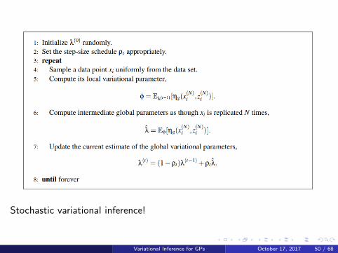
Stochastic variational inference!
Variational Inference for GPs October 17, 2017 50 / 68
The GP Variational Bound
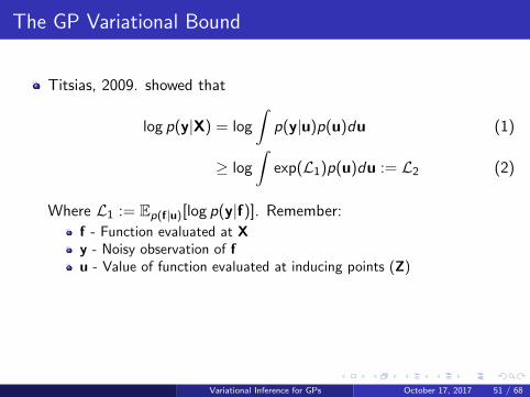
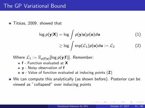
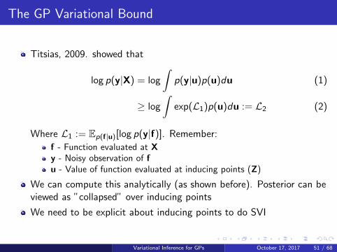
Titsias, 2009. showed that
log p(y|X) = log
∫p(y|u)p(u)du (1)
≥ log
∫exp(L1)p(u)du := L2 (2)
Where L1 := Ep(f|u)[log p(y|f)]. Remember:
f - Function evaluated at Xy - Noisy observation of fu - Value of function evaluated at inducing points (Z)
We can compute this analytically (as shown before). Posterior can beviewed as ”collapsed” over inducing points
We need to be explicit about inducing points to do SVI
Variational Inference for GPs October 17, 2017 51 / 68
The GP Variational Bound
Titsias, 2009. showed that
log p(y|X) = log
∫p(y|u)p(u)du (1)
≥ log
∫exp(L1)p(u)du := L2 (2)
Where L1 := Ep(f|u)[log p(y|f)]. Remember:
f - Function evaluated at Xy - Noisy observation of fu - Value of function evaluated at inducing points (Z)
We can compute this analytically (as shown before). Posterior can beviewed as ”collapsed” over inducing points
We need to be explicit about inducing points to do SVI
Variational Inference for GPs October 17, 2017 51 / 68
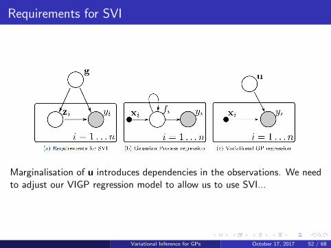
Requirements for SVI
Marginalisation of u introduces dependencies in the observations. We needto adjust our VIGP regression model to allow us to use SVI...
Variational Inference for GPs October 17, 2017 52 / 68

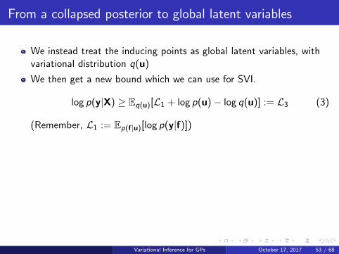
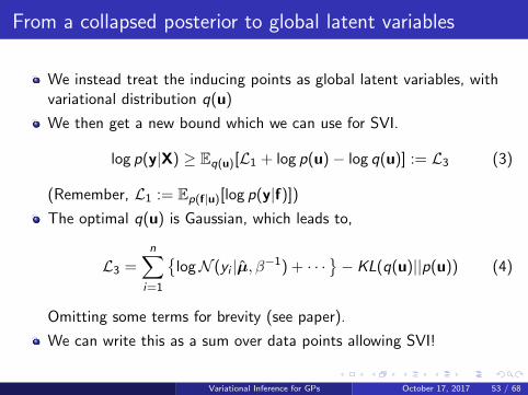
From a collapsed posterior to global latent variables
We instead treat the inducing points as global latent variables, withvariational distribution q(u)
We then get a new bound which we can use for SVI.
log p(y|X) ≥ Eq(u)[L1 + log p(u)− log q(u)] := L3 (3)
(Remember, L1 := Ep(f|u)[log p(y|f)])
The optimal q(u) is Gaussian, which leads to,
L3 =n∑
i=1
{logN (yi |µ, β−1) + · · ·
}− KL(q(u)||p(u)) (4)
Omitting some terms for brevity (see paper).
We can write this as a sum over data points allowing SVI!
Variational Inference for GPs October 17, 2017 53 / 68
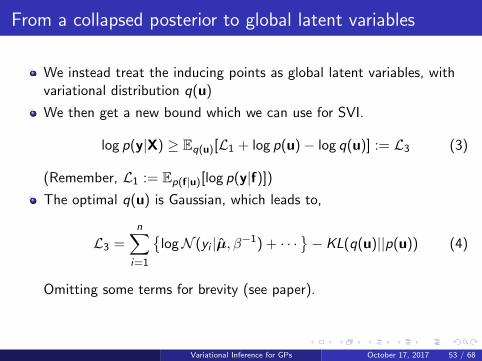
Inference with this new bound
We perform SVI using natural gradient updates
Exponential family leads to a nice form of the updates
See the paper for the derived update rules
Training updates are now O(m3)!
Can also use non-Gaussian likelihoods because of the L3 factorisation.This normally requires approximations.
Variational Inference for GPs October 17, 2017 54 / 68
Experiments I
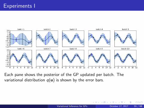
Each pane shows the posterior of the GP updated per batch. Thevariational distribution q(u) is shown by the error bars.
Variational Inference for GPs October 17, 2017 55 / 68
Experiments II
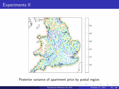
Posterior variance of apartment price by postal region.
Variational Inference for GPs October 17, 2017 56 / 68
Summary
We cannot do SVI on the collapsed VI bound.
But we can refactorize it.
SVI lets us handle big data and can attain the same optimumparameters.
Variational Inference for GPs October 17, 2017 57 / 68
Summary
We cannot do SVI on the collapsed VI bound.
But we can refactorize it.
SVI lets us handle big data and can attain the same optimumparameters.
Variational Inference for GPs October 17, 2017 57 / 68
Summary
We cannot do SVI on the collapsed VI bound.
But we can refactorize it.
SVI lets us handle big data and can attain the same optimumparameters.
Variational Inference for GPs October 17, 2017 57 / 68
PAC-Bayes
PAC-Bayes
Variational Inference for GPs October 17, 2017 58 / 68
Hoeffding’s Inequality
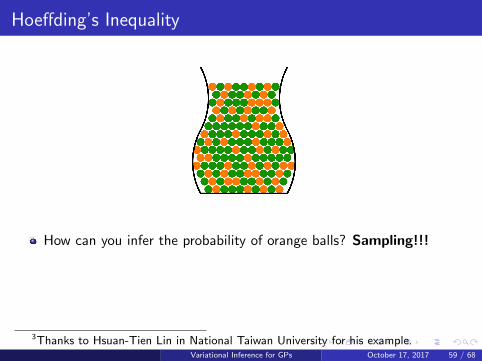
How can you infer the probability of orange balls?
Sampling!!!
Assume the real orange probability is µ, the number of balls sampledis N, the sampling orange probability is ν.How accurate is your estimation by sampling?
3
3Thanks to Hsuan-Tien Lin in National Taiwan University for his example.Variational Inference for GPs October 17, 2017 59 / 68
Hoeffding’s Inequality
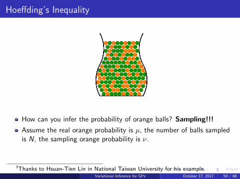
How can you infer the probability of orange balls? Sampling!!!
Assume the real orange probability is µ, the number of balls sampledis N, the sampling orange probability is ν.How accurate is your estimation by sampling?
3
3Thanks to Hsuan-Tien Lin in National Taiwan University for his example.Variational Inference for GPs October 17, 2017 59 / 68
Hoeffding’s Inequality
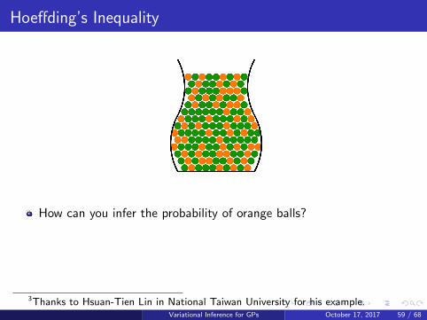
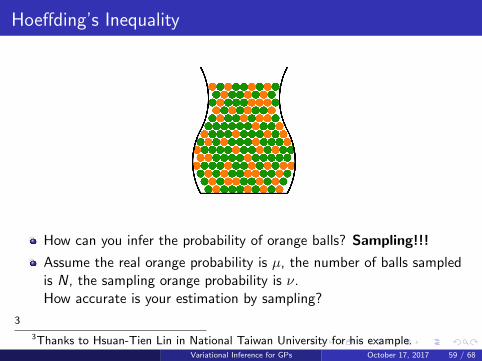
How can you infer the probability of orange balls? Sampling!!!
Assume the real orange probability is µ, the number of balls sampledis N, the sampling orange probability is ν.
How accurate is your estimation by sampling?
3
3Thanks to Hsuan-Tien Lin in National Taiwan University for his example.Variational Inference for GPs October 17, 2017 59 / 68
Hoeffding’s Inequality
How can you infer the probability of orange balls? Sampling!!!
Assume the real orange probability is µ, the number of balls sampledis N, the sampling orange probability is ν.How accurate is your estimation by sampling?
3
3Thanks to Hsuan-Tien Lin in National Taiwan University for his example.Variational Inference for GPs October 17, 2017 59 / 68
Hoeffding’s Inequality
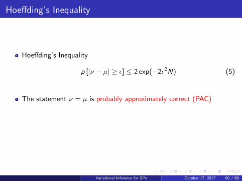
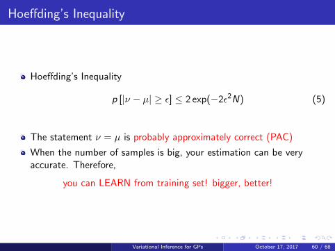
Hoeffding’s Inequality
p [|ν − µ| ≥ ε] ≤ 2 exp(−2ε2N) (5)
The statement ν = µ is probably approximately correct (PAC)
When the number of samples is big, your estimation can be veryaccurate. Therefore,
you can LEARN from training set! bigger, better!
Variational Inference for GPs October 17, 2017 60 / 68
Hoeffding’s Inequality
Hoeffding’s Inequality
p [|ν − µ| ≥ ε] ≤ 2 exp(−2ε2N) (5)
The statement ν = µ is probably approximately correct (PAC)
When the number of samples is big, your estimation can be veryaccurate. Therefore,
you can LEARN from training set! bigger, better!
Variational Inference for GPs October 17, 2017 60 / 68
Hoeffding’s Inequality
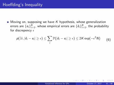
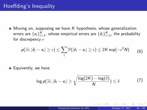
Moving on, supposing we have K hypothesis, whose generalizationerrors are {ei}K
i=1, whose empirical errors are {ei}Ki=1, the probability
for discrepency ε
p(∃i , |ei − ei | ≥ ε) ≤∑
i
P(|ei − ei | ≥ ε) ≤ 2K exp(−ε2N) (6)
Equivently, we have
log p(∃i , |ei − ei | ≥√
log(2K )− log(δ)
N) ≤ δ (7)
Variational Inference for GPs October 17, 2017 61 / 68
Hoeffding’s Inequality
Moving on, supposing we have K hypothesis, whose generalizationerrors are {ei}K
i=1, whose empirical errors are {ei}Ki=1, the probability
for discrepency ε
p(∃i , |ei − ei | ≥ ε) ≤∑
i
P(|ei − ei | ≥ ε) ≤ 2K exp(−ε2N) (6)
Equivently, we have
log p(∃i , |ei − ei | ≥√
log(2K )− log(δ)
N) ≤ δ (7)
Variational Inference for GPs October 17, 2017 61 / 68
Gibbs Classifier Bayes Classifier
Suppose we’re doing a binary classification task. Let x ∈ X andt ∈ {−1, 1}.The model is composed of a latent function x→ y(x), and aclassification model P(t|y).
From the Bayesian viewpoint, the latent function could beparametrized as y(x|w), where w ∼ Q(w)
Variational Inference for GPs October 17, 2017 62 / 68
Gibbs Classifier Bayes Classifier
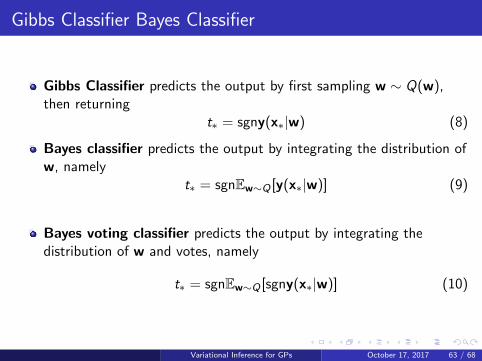
Gibbs Classifier predicts the output by first sampling w ∼ Q(w),then returning
t∗ = sgny(x∗|w) (8)
Bayes classifier predicts the output by integrating the distribution ofw, namely
t∗ = sgnEw∼Q [y(x∗|w)] (9)
Bayes voting classifier predicts the output by integrating thedistribution of w and votes, namely
t∗ = sgnEw∼Q [sgny(x∗|w)] (10)
Variational Inference for GPs October 17, 2017 63 / 68
Gibbs Classifier Bayes Classifier
Gibbs Classifier predicts the output by first sampling w ∼ Q(w),then returning
t∗ = sgny(x∗|w) (8)
Bayes classifier predicts the output by integrating the distribution ofw, namely
t∗ = sgnEw∼Q [y(x∗|w)] (9)
Bayes voting classifier predicts the output by integrating thedistribution of w and votes, namely
t∗ = sgnEw∼Q [sgny(x∗|w)] (10)
Variational Inference for GPs October 17, 2017 63 / 68
PAC-Bayesian theorem (McAllester, 1999)
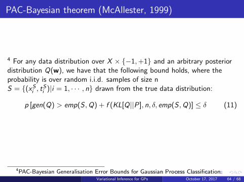
4 For any data distribution over X × {−1,+1} and an arbitrary posteriordistribution Q(w), we have that the following bound holds, where theprobability is over random i.i.d. samples of size nS = {(xS
i , tSi )|i = 1, · · · , n} drawn from the true data distribution:
p [gen(Q) > emp(S ,Q) + f (KL[Q||P], n, δ, emp(S ,Q)] ≤ δ (11)
4PAC-Bayesian Generalisation Error Bounds for Gaussian Process ClassificationVariational Inference for GPs October 17, 2017 64 / 68

PAC-Bayesian theorem (McAllester, 1999)
4 For any data distribution over X × {−1,+1} and an arbitrary posteriordistribution Q(w), we have that the following bound holds, where theprobability is over random i.i.d. samples of size nS = {(xS
i , tSi )|i = 1, · · · , n} drawn from the true data distribution:
p [gen(Q) > emp(S ,Q) + f (KL[Q||P], n, δ, emp(S ,Q)] ≤ δ (11)
4PAC-Bayesian Generalisation Error Bounds for Gaussian Process ClassificationVariational Inference for GPs October 17, 2017 64 / 68
Variational Inference and PAC-Bayesian
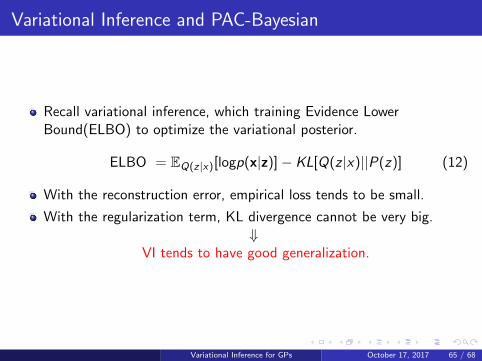
Recall variational inference, which training Evidence LowerBound(ELBO) to optimize the variational posterior.
ELBO = EQ(z|x)[logp(x|z)]− KL[Q(z |x)||P(z)] (12)
With the reconstruction error, empirical loss tends to be small.
With the regularization term, KL divergence cannot be very big.⇓
VI tends to have good generalization.
Variational Inference for GPs October 17, 2017 65 / 68
Gaussian Process Classification
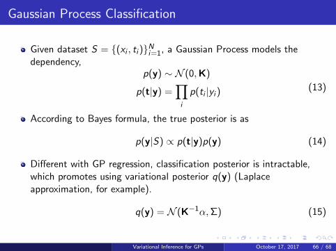
Given dataset S = {(xi , ti )}Ni=1, a Gaussian Process models the
dependency,p(y) ∼ N (0,K)
p(t|y) =∏
i
p(ti |yi )(13)
According to Bayes formula, the true posterior is as
p(y|S) ∝ p(t|y)p(y) (14)
Different with GP regression, classification posterior is intractable,which promotes using variational posterior q(y) (Laplaceapproximation, for example).
q(y) = N (K−1α,Σ) (15)
Variational Inference for GPs October 17, 2017 66 / 68
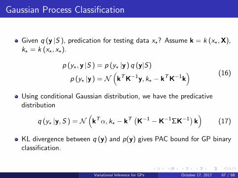
Gaussian Process Classification
Given q (y |S ), predication for testing data x?? Assume k = k (x?,X),k? = k (x?, x?).
p (y?, y |S ) = p (y? |y ) q (y|S)
p (y? |y ) = N(
kT K−1y, k? − kT K−1k) (16)
Using conditional Gaussian distribution, we have the predicativedistribution
q (y? |y, S ) = N(
kTα, k? − kT(K−1 −K−1ΣK−1
)k)
(17)
KL divergence between q (y) and p(y) gives PAC bound for GP binaryclassification.
Variational Inference for GPs October 17, 2017 67 / 68
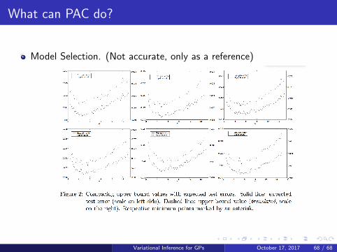
What can PAC do?
Model Selection. (Not accurate, only as a reference)
Variational Inference for GPs October 17, 2017 68 / 68