Embed Size (px)
Citation preview
Vector Autoregressions as a Guide to ConstructingDynamic General Equilibrium Models
by
Lawrence J. Christiano, Martin Eichenbaum and Robert Vigfusson
1
Background
• We Use VAR Impulse Response Functions as Guide to Constructing MonetaryDSGE Models– Basic Strategy: Choose Model Parameters to Make Model-based Impulse
Responses as Close as Possible to VAR-based Impulse Responses.• Problem: The Usefulness of Vector Autoregressions Has Been Questioned• For Example: CKM Question the Use of VARs with Long-Run Restrictions....
– CKM Argue (as do Others) That First Differencing Hours Worked WhenHours are Stationary Can Lead to Incorrect VAR Inference (DSVARS)
– Here, We are Concerned With their Findings for LSVARS, When Hours areCorrectly Specified in Levels
– CKM Report Two Major Findings.∗ VARs Increasingly Distorted and Misleading as Datasets Grow· We Do Not Find This.
∗ VARs Are Uninformative in Small Samples.· We Disagree.
12
Findings
• All Findings Based on Running VARs in Data Generated by DSGE Models.• Long-Run Exclusion and Sign Restrictions
– Our Examples: As Long As there are Enough Variables in the Analysis -∗ Inference from VARs Reliable.∗ There May be Substantial Sampling Uncertainty· But, A Conceptual Error Leads CKM to Greatly Overstate that
Uncertainty.
∗ In Any Case, VAR Methods Accurately Characterize Uncertainty.∗ A User of VARs Would Not Be Misled in Practice
• Short-Run Exclusion and Sign Restrictions– Our Examples Suggest∗ No Evidence of Small-Sample Bias∗ Relatively Little Sampling Uncertainty∗ Robust to Which Variables are Included in VAR
20
Outline
• Analysis Based on Simple RBC Model– Long Run Restrictions
– Short Run Restrictions
• Analysis Based on Monetized RBC Models With Various Frictions (ACEL)
18
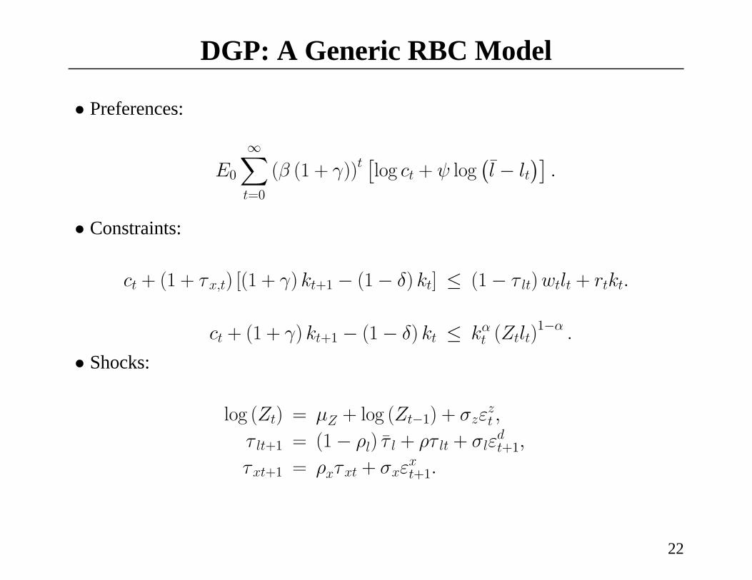
DGP: A Generic RBC Model
• Preferences:
E0
∞Xt=0
(β (1 + γ))t£log ct + ψ log
¡l̄ − lt
¢¤.
• Constraints:
ct + (1 + τx,t) [(1 + γ) kt+1 − (1− δ) kt] ≤ (1− τ lt)wtlt + rtkt.
ct + (1 + γ) kt+1 − (1− δ) kt ≤ kαt (Ztlt)1−α .
• Shocks:
log (Zt) = µZ + log (Zt−1) + σzεzt ,
τ lt+1 = (1− ρl) τ̄ l + ρτ lt + σlεdt+1,
τxt+1 = ρxτxt + σxεxt+1.
22
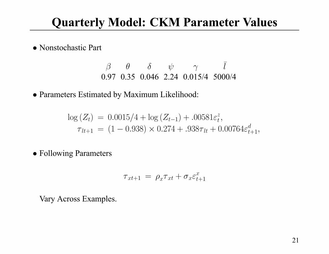
Quarterly Model: CKM Parameter Values
• Nonstochastic Part
¯
0.97 0.35 0.046 2.24 0.015/4 5000/4
• Parameters Estimated by Maximum Likelihood:
log ( ) = 0 0015 4 + log ( 1) + 00581
+1 = (1 0 938)× 0 274 + 938 + 0 00764 +1
• Following Parameters
+1 = + +1
Vary Across Examples.
21
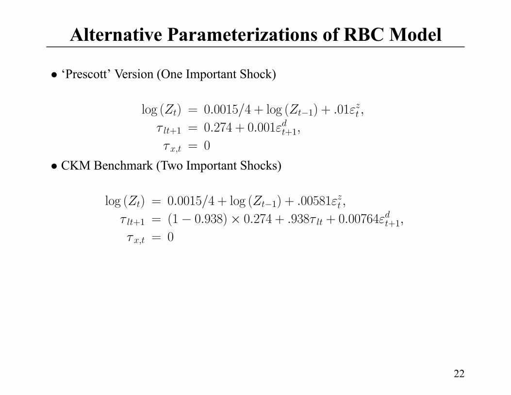
Alternative Parameterizations of RBC Model
• ‘Prescott’ Version (One Important Shock)
log ( ) = 0 0015 4 + log ( 1) + 01
+1 = 0 274 + 0 001 +1
= 0
• CKM Benchmark (Two Important Shocks)
log ( ) = 0 0015 4 + log ( 1) + 00581
+1 = (1 0 938)× 0 274 + 938 + 0 00764 +1
= 0
22
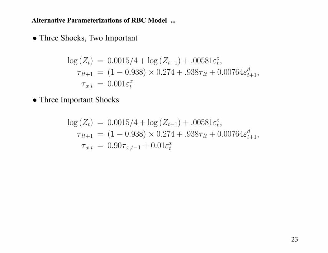
Alternative Parameterizations of RBC Model ...
• Three Shocks, Two Important
log ( ) = 0 0015 4 + log ( 1) + 00581
+1 = (1 0 938)× 0 274 + 938 + 0 00764 +1
= 0 001
• Three Important Shocks
log ( ) = 0 0015 4 + log ( 1) + 00581
+1 = (1 0 938)× 0 274 + 938 + 0 00764 +1
= 0 90 1 + 0 01
23
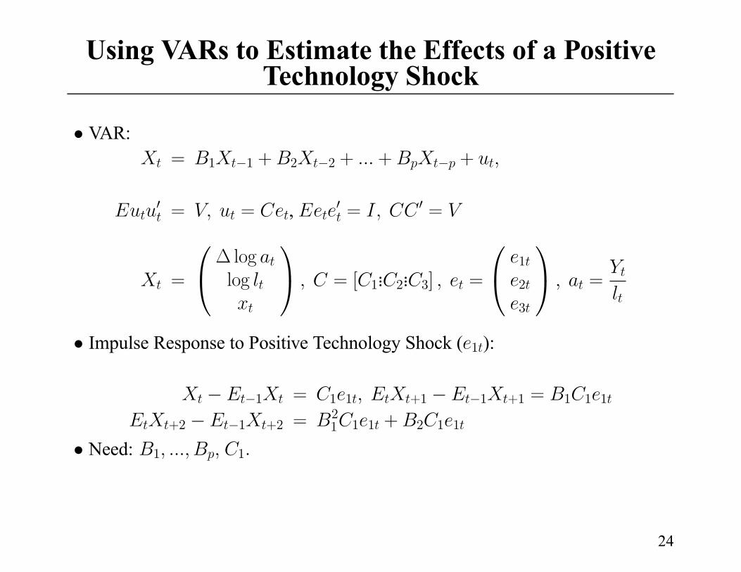
Using VARs to Estimate the Effects of a PositiveTechnology Shock
• VAR:
= 1 1 + 2 2 + + +
0 = = , 0 = 0 =
=loglog = [ 1
... 2... 3] =
1
2
3
=
• Impulse Response to Positive Technology Shock ( 1 ):
1 = 1 1 +1 1 +1 = 1 1 1
+2 1 +2 =21 1 1 + 2 1 1
• Need: 1 1
24
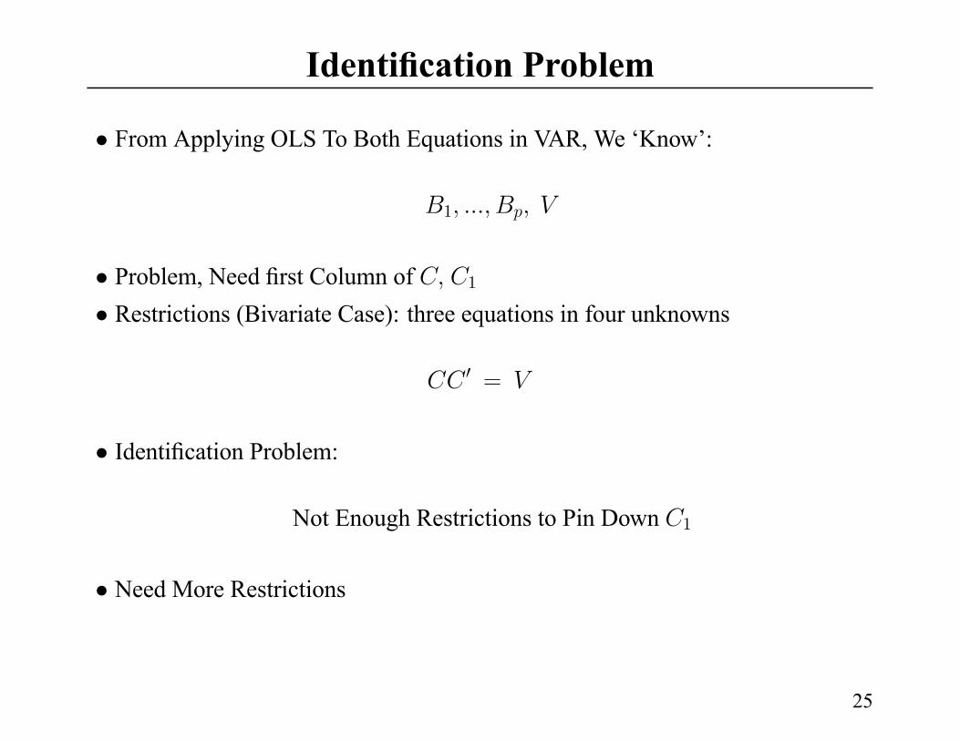
Identification Problem
• From Applying OLS To Both Equations in VAR, We ‘Know’:
1
• Problem, Need first Column of 1
• Restrictions (Bivariate Case): three equations in four unknowns
0 =
• Identification Problem:
Not Enough Restrictions to Pin Down 1
• Need More Restrictions
25
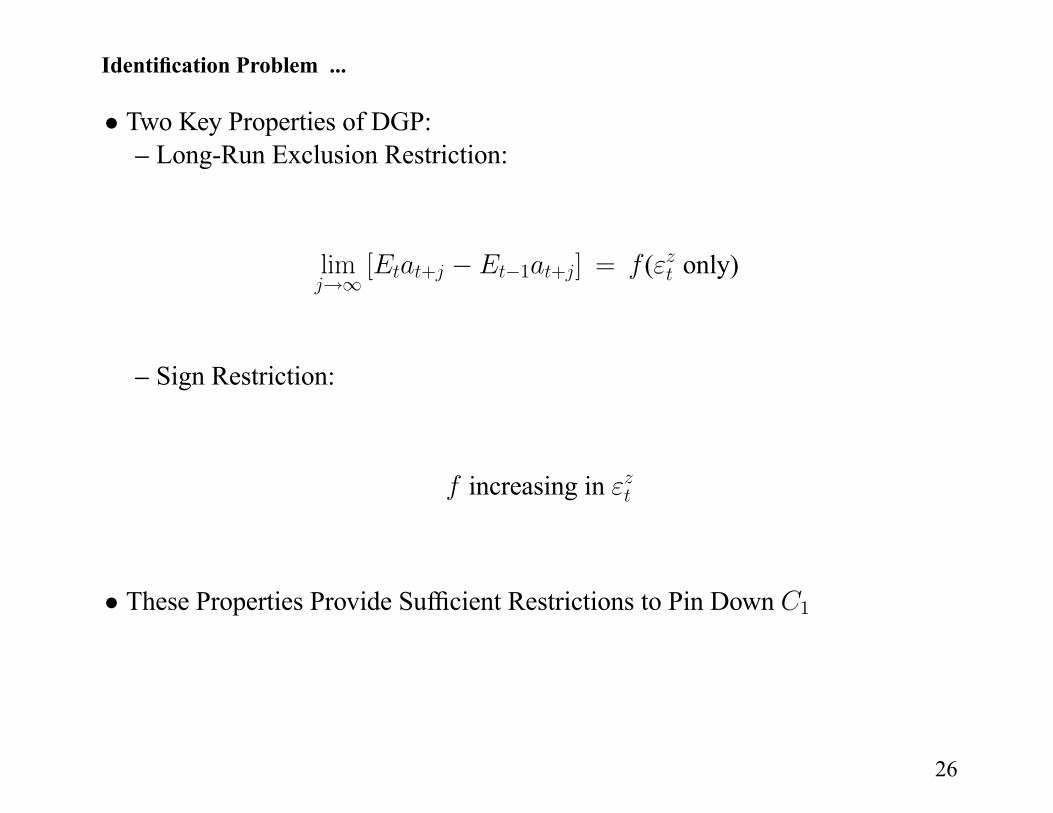
Identification Problem ...
• Two Key Properties of DGP:– Long-Run Exclusion Restriction:
lim [ + 1 + ] = ( only)
– Sign Restriction:
increasing in
• These Properties Provide Sufficient Restrictions to Pin Down 1
26
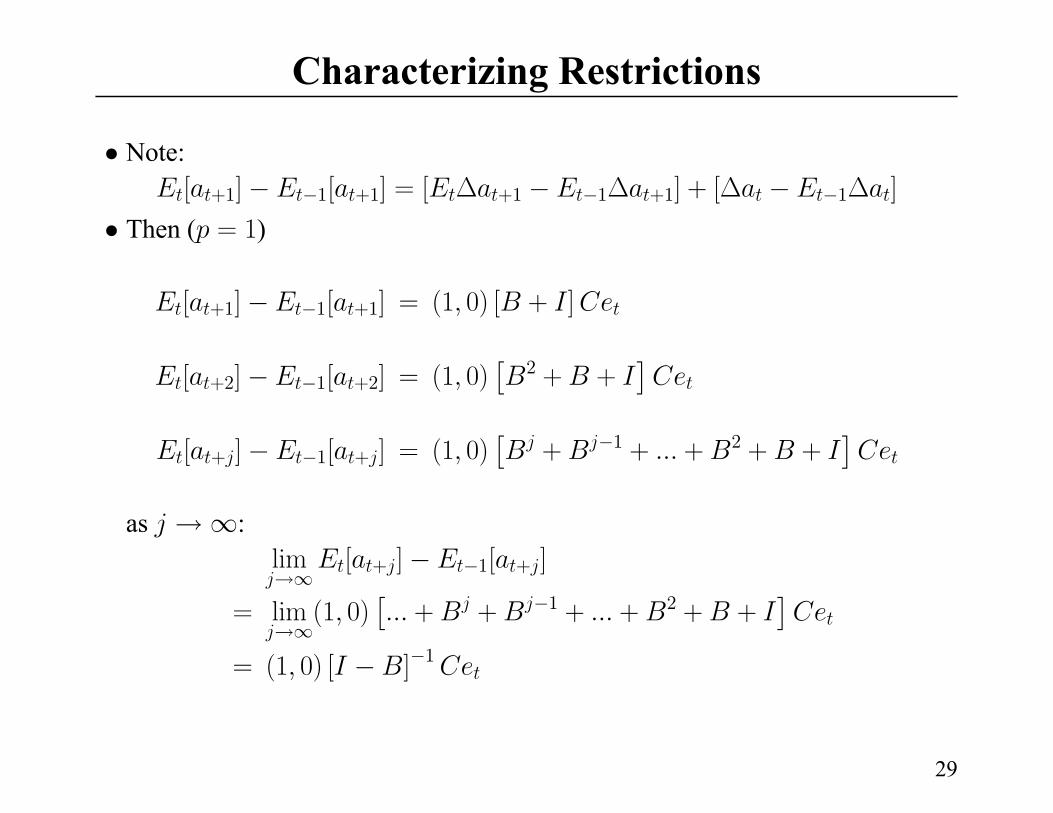
Characterizing Restrictions
• Note:
[ +1] 1[ +1] = [ +1 1 +1] + [ 1 ]
• Then ( = 1)
[ +1] 1[ +1] = (1 0) [ + ]
[ +2] 1[ +2] = (1 0)£
2 + +¤
[ + ] 1[ + ] = (1 0)£
+ 1 + + 2 + +¤
as :
lim [ + ] 1[ + ]
= lim (1 0)£+ + 1 + + 2 + +
¤= (1 0) [ ] 1
29

Characterizing Restrictions ...
• As j →∞ (for arbitrary p) :
limj→∞
Et[at+j]−Et−1[at+j] = (1, 0) [I −B(1)]−1Cet
37
Characterizing Restrictions ...
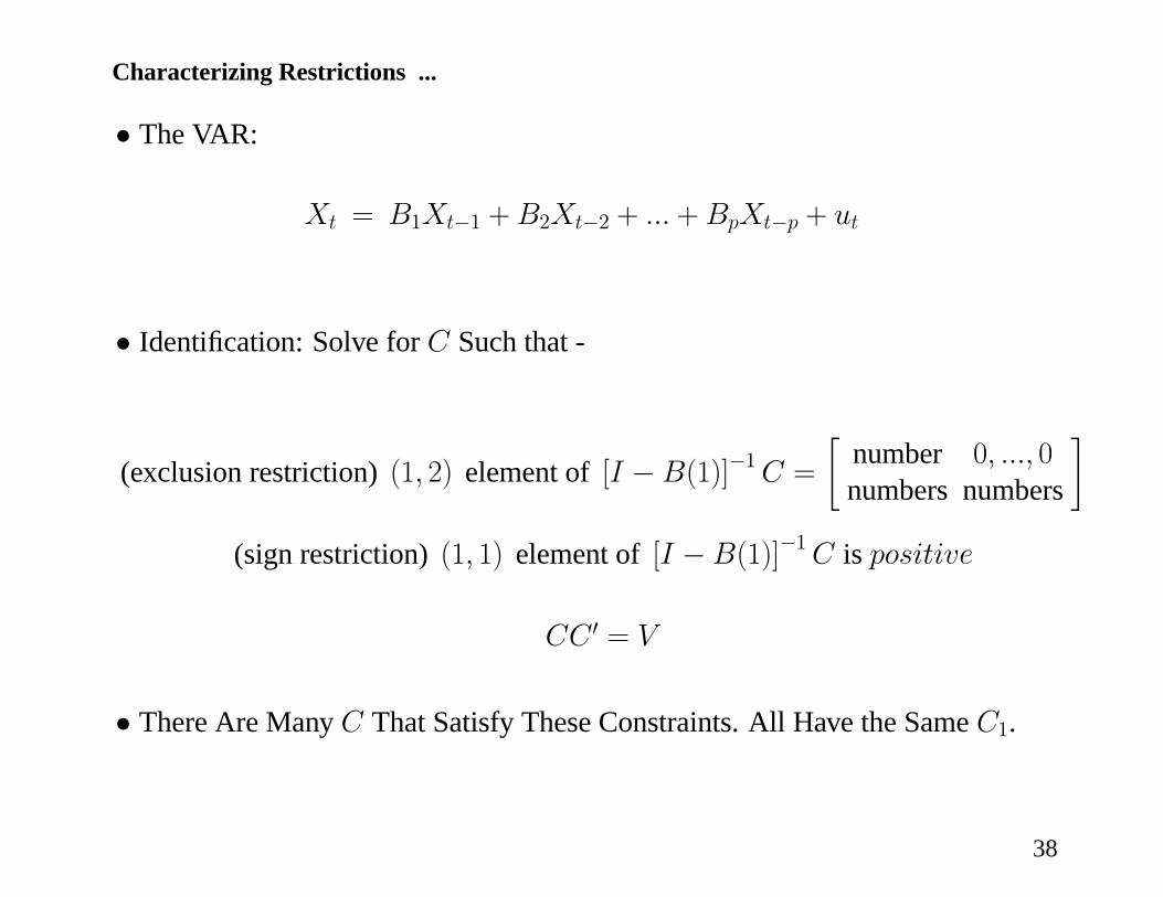
• The VAR:
Xt = B1Xt−1 +B2Xt−2 + ... +BpXt−p + ut
• Identification: Solve for C Such that -
(exclusion restriction) (1, 2) element of [I −B(1)]−1C =
∙number 0, ..., 0numbers numbers
¸(sign restriction) (1, 1) element of [I −B(1)]−1C is positive
CC 0 = V
• There Are Many C That Satisfy These Constraints. All Have the Same C1.
38
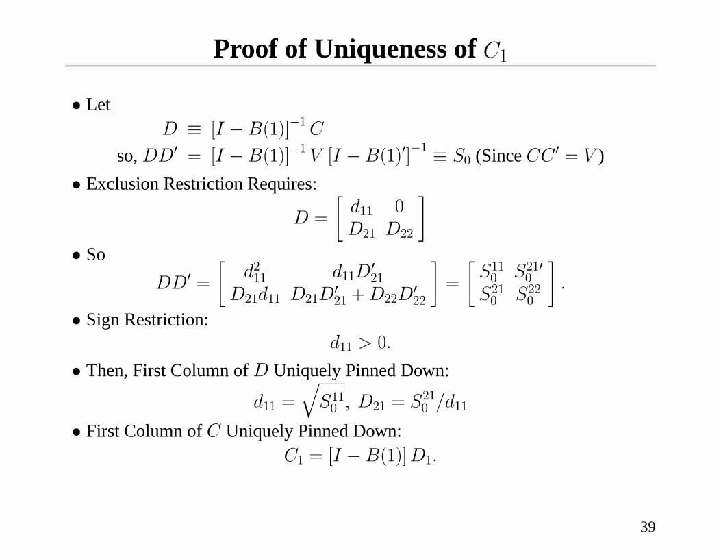
Proof of Uniqueness of C1
• LetD ≡ [I −B(1)]−1C
so, DD0 = [I −B(1)]−1 V [I −B(1)0]−1 ≡ S0 (Since CC 0 = V )
• Exclusion Restriction Requires:
D =
∙d11 0D21 D22
¸• So
DD0 =
∙d211 d11D
021
D21d11 D21D021 +D22D
022
¸=
∙S110 S2100S210 S220
¸.
• Sign Restriction:d11 > 0.
• Then, First Column of D Uniquely Pinned Down:
d11 =qS110 , D21 = S210 /d11
• First Column of C Uniquely Pinned Down:C1 = [I −B(1)]D1.
39

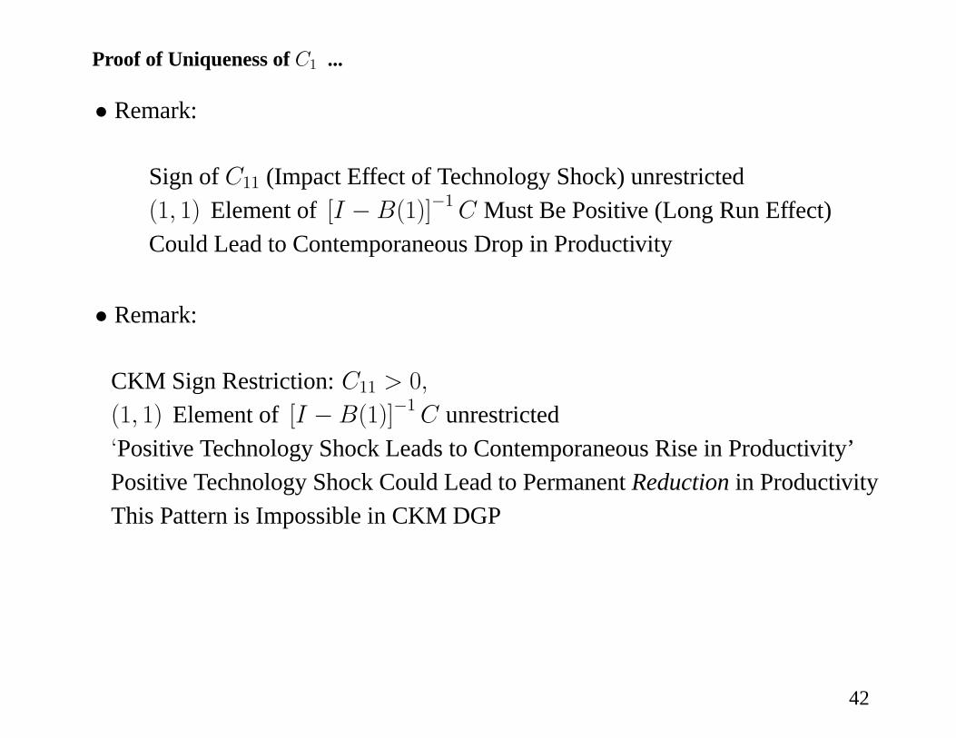
Proof of Uniqueness of C1 ...
• Remark:
Sign of C11 (Impact Effect of Technology Shock) unrestricted(1, 1) Element of [I −B(1)]−1C Must Be Positive (Long Run Effect)Could Lead to Contemporaneous Drop in Productivity
41
Proof of Uniqueness of C1 ...
• Remark:
Sign of C11 (Impact Effect of Technology Shock) unrestricted(1, 1) Element of [I −B(1)]−1C Must Be Positive (Long Run Effect)Could Lead to Contemporaneous Drop in Productivity
• Remark:
CKM Sign Restriction: C11 > 0,(1, 1) Element of [I −B(1)]−1C unrestricted‘Positive Technology Shock Leads to Contemporaneous Rise in Productivity’Positive Technology Shock Could Lead to Permanent Reduction in ProductivityThis Pattern is Impossible in CKM DGP
42
Assessing the VARWith Long-Run RestrictionsUsing RBC as DGP
• Experiments– Simulate 500 Artificial Data Sets, Each of Length 180 From Various
Versions of DGP
– Estimate VAR On Each Artificial Data Set and Compute Dynamic Response
of Hours to Positive Technology Shock
– Report Mean Impulse Response Function and Plus/Minus Two Standard
Error Bounds (Grey Area)
39
Assessing the VARWith Long-Run Restrictions Using RBC as DGP ...
• General Findings:– If there are Enough Variables, Relative to the Number of Important Shocks
to the Economy, then VAR Reliable
Precision May be Low, But VAR Will Tell You When this is So.
Often, But not Always, One Can Discriminate Between Interesting
Hypotheses
– CKM Finding of Enormous Sampling Uncertainty Reflects CKM’s
Mistaken Sign Restriction
–We are Less Pessimistic than CKM About What Happens as More Data
Come In
(These Findings are Somewhat Tentative, Until We Fully Understand
Why Our Results Differ from CKM.)
42
Notes on Figures 0 and 1
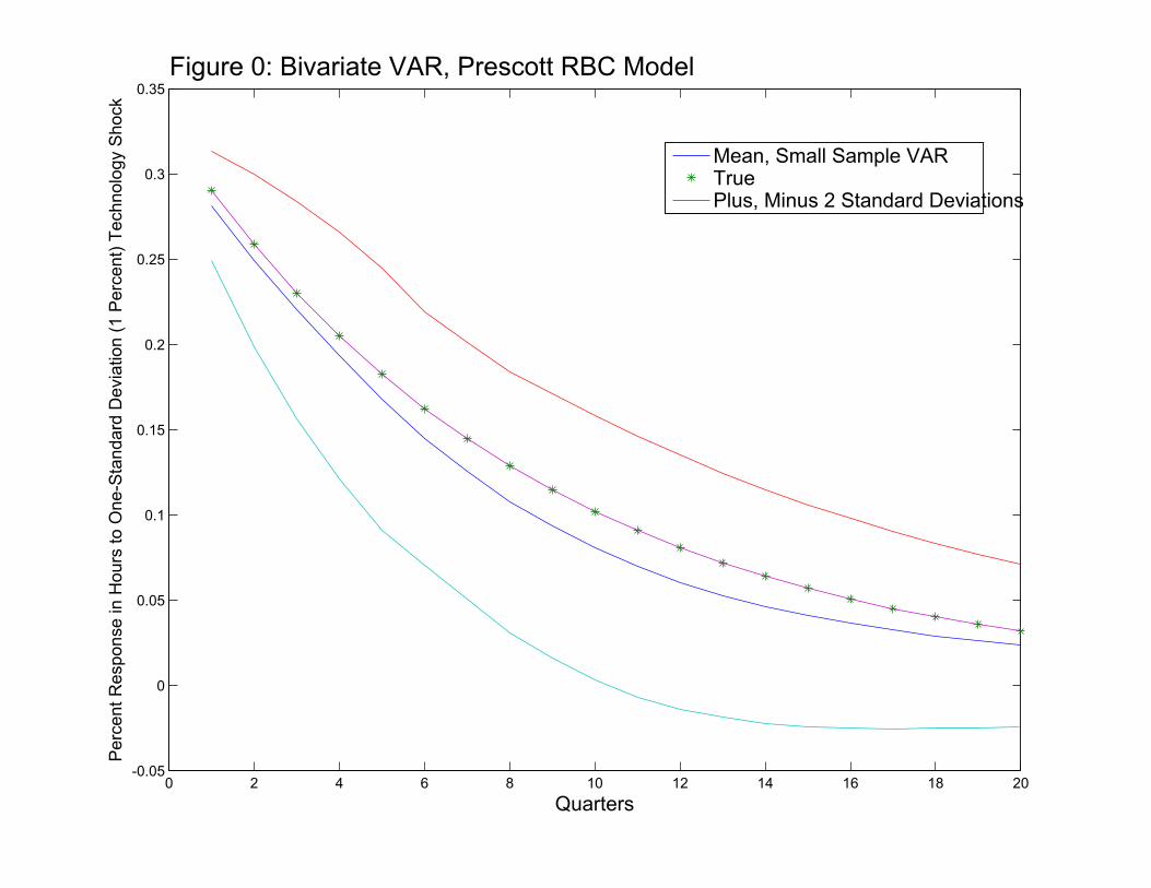
• Figure 0:– ‘Prescott’ RBCModel with Standard Deviation, 0.01, on Technology Shock
Other Shocks Tiny:
+1 = 0
+1 = 0 274 + 0 001× +1
Range of Impulse Responses Small
· If the Model is True, Econometrician Would Reject InterestingAlternatives (e.g., King-Wolman and Francis-Ramey Models in
Which Hours Fall After Technology Shock).
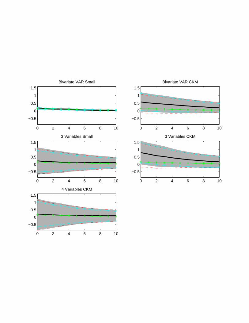
· This presumes that +/- 2 standard deviation bounds in Figure 0corresponds to confidence intervals that an econometrician would
find if the model were true. In fact, Figure 2 indicates that this is a
reasonable approximation. Fig 2 reports the actual standard deviation
of econometrician’s estimator of the impulse response function (light
blue line with dots) as well as the mean (and plus/minus two standard
error bands) of the econometrician’s bootstrap estimator of standard
43

Notes on Figures 0 and 1 ...
deviation.
– Impulse Response Functions Estimated Very Tightly
– Can Easily Exclude Interesting Alternatives
44
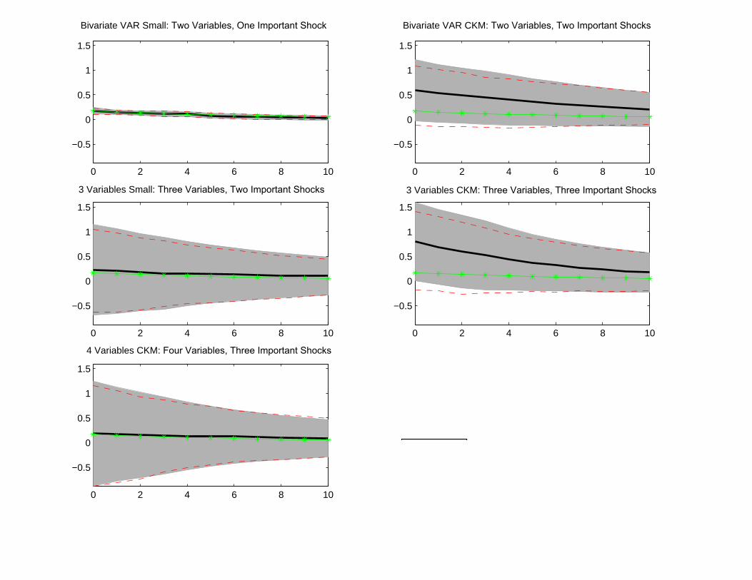
Notes on Figures 0 and 1 ...
• Figure 1:– 1,1 Element: “Two Variables, One Important Shock”
CKM Estimated Technology Shock Process
Other Shocks Tiny:
+1 = 0
+1 = 0 274 + 0 001× +1
Same as in Figure 0
– 1,2 Element: “Two Variables, Two Important Shocks” - Benchmark CKM
Example
CKM Estimated Technology and Labor Tax Shocks
+1 = 0
Substantial Small Sample Bias
Sampling Uncertainty Reported Here VERY Different from That
Reported for Same Example in CKM (Will Return to this Below).
45
Notes on Figures 0 and 1 ...
– 2,1 Element: “Three Variables, Two Important Shocks”
CKM Estimated Technology and Labor Tax Shock Process
Investment Price Shock:
+1 = 0 001× +1
VAR Bias Disappears.
Sampling Uncertainty Higher, Harder to Reject Interesting Hypotheses
– 2,2 Element: “Three Variables, Three Important Shocks”
CKM Estimated Technology and Labor Tax Process
CKM Price of Investment Example:
+1 = 0 90 + 0 01× +1
Small Sample Bias Reappears
46
Notes on Figures 0 and 1 ...
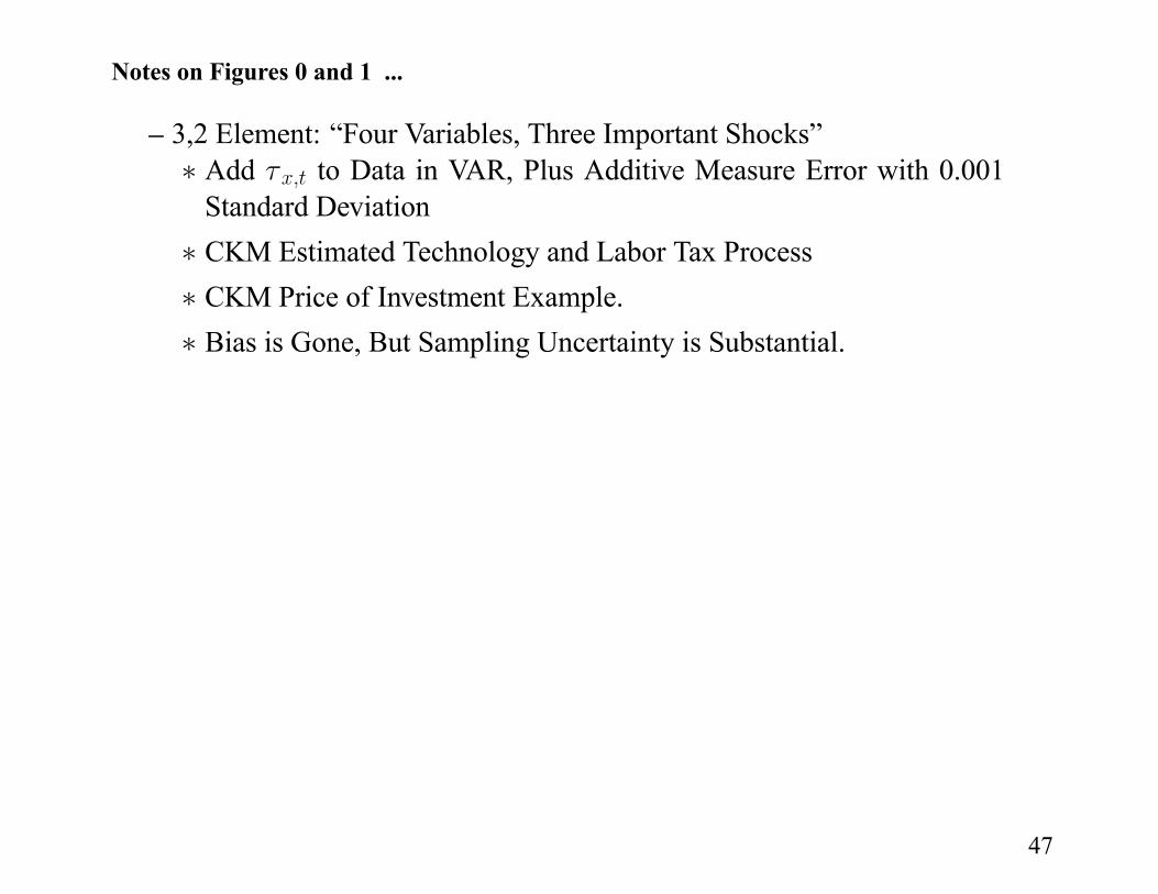
– 3,2 Element: “Four Variables, Three Important Shocks”
Add to Data in VAR, Plus Additive Measure Error with 0.001
Standard Deviation
CKM Estimated Technology and Labor Tax Process
CKM Price of Investment Example.
Bias is Gone, But Sampling Uncertainty is Substantial.
47
0 2 4 6 8 10 12 14 16 18 20-0.05
0
0.05
0.1
0.15
0.2
0.25
0.3
0.35
Quarters
Perc
ent
Response in H
ours
to O
ne-S
tandard
Devia
tion (
1 P
erc
ent)
Technolo
gy S
hock
Figure 0: Bivariate VAR, Prescott RBC Model
Mean, Small Sample VARTruePlus, Minus 2 Standard Deviations
0 2 4 6 8 10
−0.5
0
0.5
1
1.5
Bivariate VAR Small: Two Variables, One Important Shock
0 2 4 6 8 10
−0.5
0
0.5
1
1.5
Bivariate VAR CKM: Two Variables, Two Important Shocks
0 2 4 6 8 10
−0.5
0
0.5
1
1.5
3 Variables Small: Three Variables, Two Important Shocks
0 2 4 6 8 10
−0.5
0
0.5
1
1.5
3 Variables CKM: Three Variables, Three Important Shocks
0 2 4 6 8 10
−0.5
0
0.5
1
1.5
4 Variables CKM: Four Variables, Three Important Shocks
0 2 4 6 8 10
−0.5
0
0.5
1
1.5
Bivariate VAR Small
0 2 4 6 8 10
−0.5
0
0.5
1
1.5
Bivariate VAR CKM
0 2 4 6 8 10
−0.5
0
0.5
1
1.5
3 Variables Small
0 2 4 6 8 10
−0.5
0
0.5
1
1.5
3 Variables CKM
0 2 4 6 8 10
−0.5
0
0.5
1
1.5
4 Variables CKM
What We Learn From the Examples in Figures 0and 1:
• Tentative Conclusion: VAR Inference With Long-Run Identification NotMisleading As Long as there Are “Enough” Variables in the Analysis.
– Need at Least One More Variable than the Number of Important Shocks
Driving the Data
– In Practice: Roughly 4-5 Variables (see Sargent-Sims, Quah-Sargent, Uhlig
(‘What moves real GDP?’), who show that 3-4 shocks account for most
fluctuations; see Prescott (1986) who argues 1 shock account for 70% of
fluctuations.).
50
How Big is the Sampling Uncertainty Associatedwith Long-Run Identifying Restrictions?
• CKM Provide a Misleading Answer to this Question
• Problem: CKM Sign Restriction Leads Them To Confuse Positive and
Negative Technology Shocks
51
How Big is the Sampling Uncertainty Associated with Long-Run Identifying Restrictions? ...
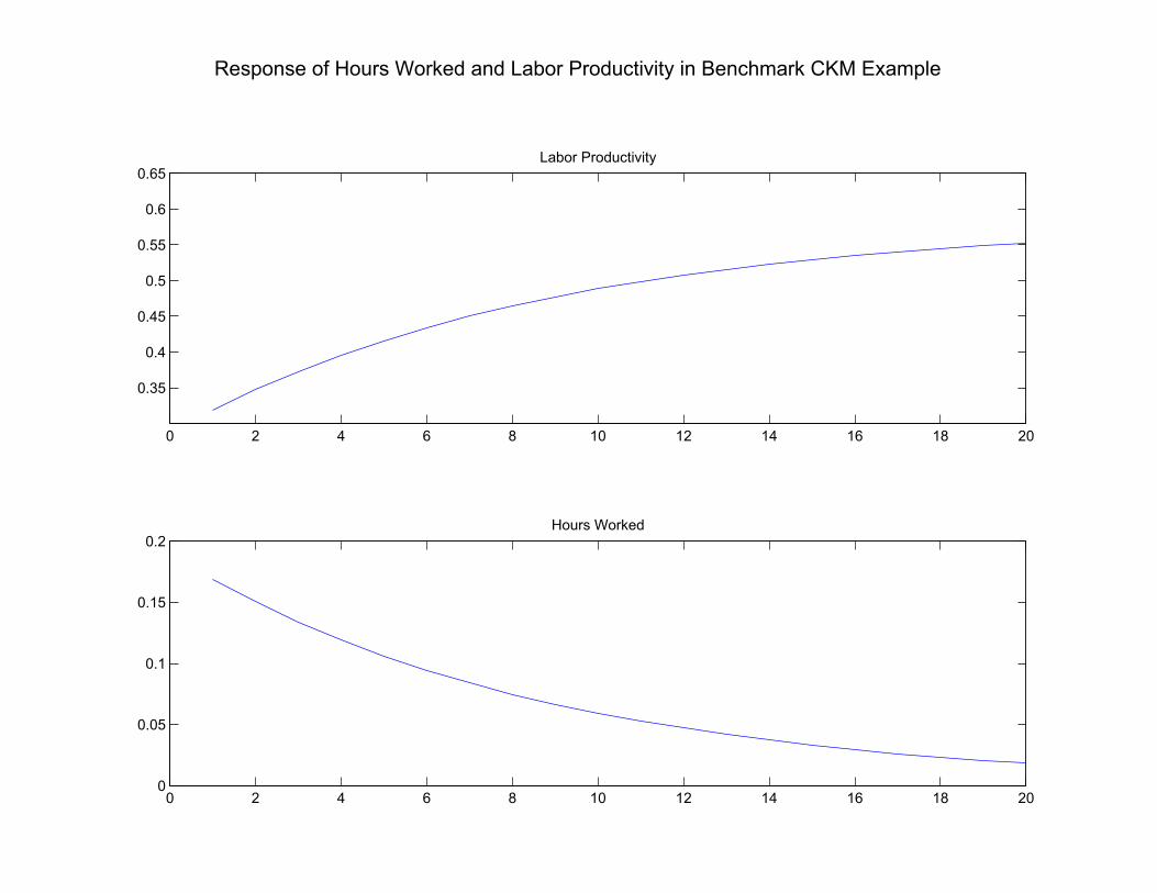
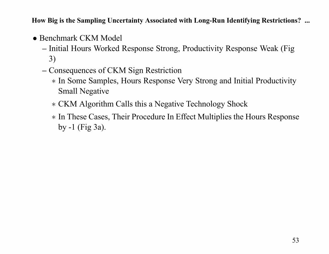
• Benchmark CKMModel– Initial Hours Worked Response Strong, Productivity Response Weak (Fig
3)
52
0 2 4 6 8 10 12 14 16 18 20
0.35
0.4
0.45
0.5
0.55
0.6
0.65Labor Productivity
Response of Hours Worked and Labor Productivity in Benchmark CKM Example
0 2 4 6 8 10 12 14 16 18 200
0.05
0.1
0.15
0.2Hours Worked
How Big is the Sampling Uncertainty Associated with Long-Run Identifying Restrictions? ...
• Benchmark CKMModel– Initial Hours Worked Response Strong, Productivity Response Weak (Fig
3)
– Consequences of CKM Sign Restriction
In Some Samples, Hours Response Very Strong and Initial Productivity
Small Negative
CKM Algorithm Calls this a Negative Technology Shock
In These Cases, Their Procedure In Effect Multiplies the Hours Response
by -1 (Fig 3a).
53
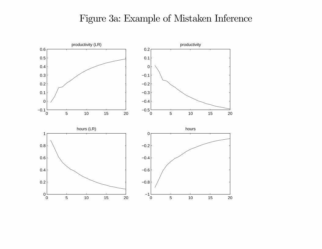
Figure 3a: Example of Mistaken Inference
0 5 10 15 20−0.1
0
0.1
0.2
0.3
0.4
0.5
0.6productivity (LR)
0 5 10 15 200
0.2
0.4
0.6
0.8
1hours (LR)
0 5 10 15 20−0.5
−0.4
−0.3
−0.2
−0.1
0
0.1
0.2productivity
0 5 10 15 20−1
−0.8
−0.6
−0.4
−0.2
0hours
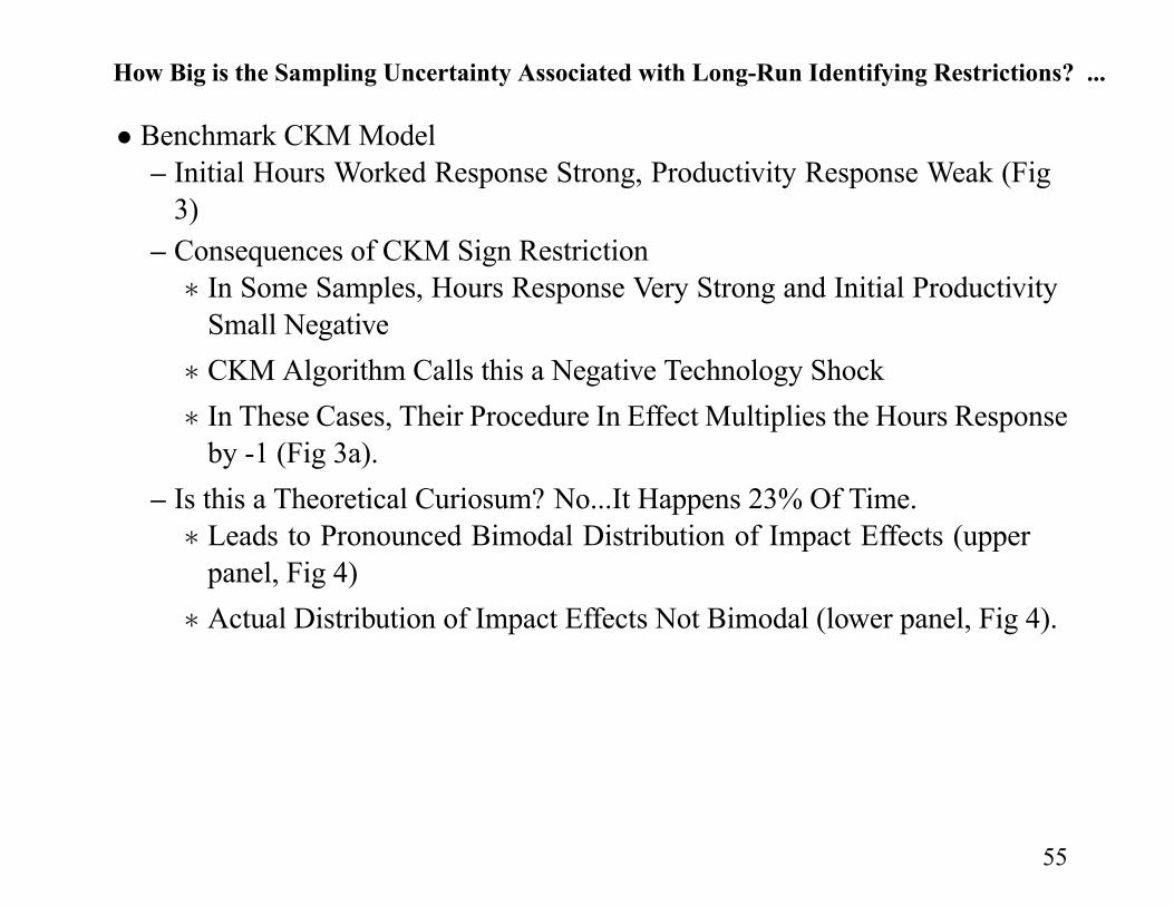
How Big is the Sampling Uncertainty Associated with Long-Run Identifying Restrictions? ...
• Benchmark CKMModel– Initial Hours Worked Response Strong, Productivity Response Weak (Fig
3)
– Consequences of CKM Sign Restriction
In Some Samples, Hours Response Very Strong and Initial Productivity
Small Negative
CKM Algorithm Calls this a Negative Technology Shock
In These Cases, Their Procedure In Effect Multiplies the Hours Response
by -1 (Fig 3a).
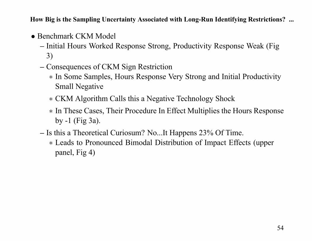
– Is this a Theoretical Curiosum? No...It Happens 23% Of Time.
Leads to Pronounced Bimodal Distribution of Impact Effects (upper
panel, Fig 4)
54
−0.02 −0.01 0 0.01 0.020
10
20
30
40
50
60
70
80
90
100Hours Impact
0 10 20 30 40 50−0.01
−0.008
−0.006
−0.004
−0.002
0
0.002
0.004
0.006
0.008
0.01Labor Productivity Response
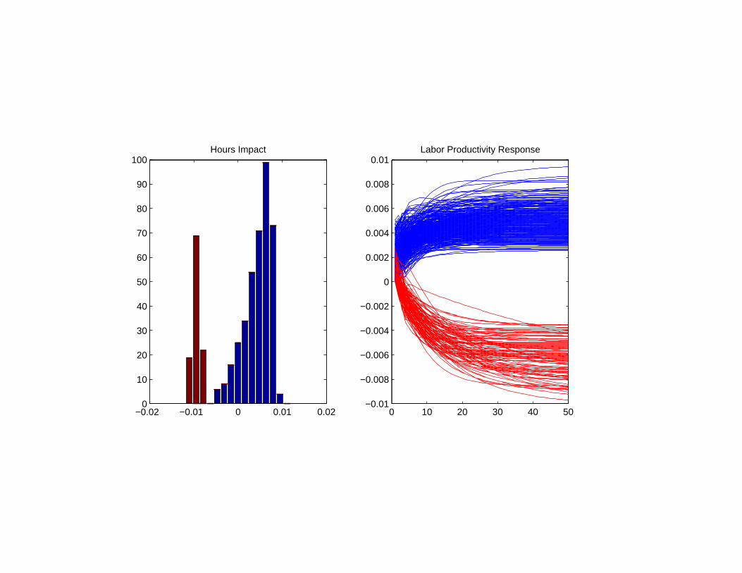
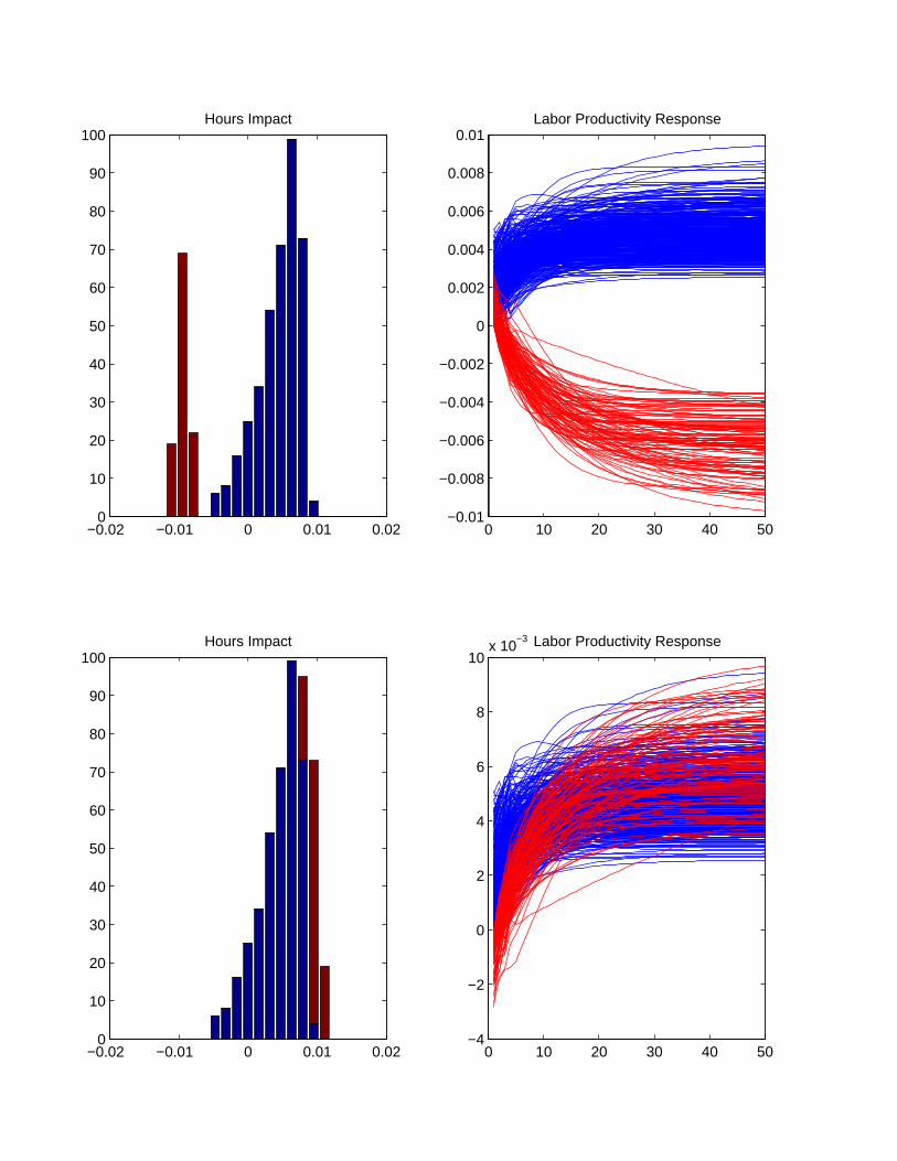
How Big is the Sampling Uncertainty Associated with Long-Run Identifying Restrictions? ...
• Benchmark CKMModel– Initial Hours Worked Response Strong, Productivity Response Weak (Fig
3)
– Consequences of CKM Sign Restriction
In Some Samples, Hours Response Very Strong and Initial Productivity
Small Negative
CKM Algorithm Calls this a Negative Technology Shock
In These Cases, Their Procedure In Effect Multiplies the Hours Response
by -1 (Fig 3a).
– Is this a Theoretical Curiosum? No...It Happens 23% Of Time.
Leads to Pronounced Bimodal Distribution of Impact Effects (upper
panel, Fig 4)
Actual Distribution of Impact Effects Not Bimodal (lower panel, Fig 4).
55
−0.02 −0.01 0 0.01 0.020
10
20
30
40
50
60
70
80
90
100Hours Impact
0 10 20 30 40 50−0.01
−0.008
−0.006
−0.004
−0.002
0
0.002
0.004
0.006
0.008
0.01Labor Productivity Response
−0.02 −0.01 0 0.01 0.020
10
20
30
40
50
60
70
80
90
100Hours Impact
0 10 20 30 40 50−4
−2
0
2
4
6
8
10x 10
−3 Labor Productivity Response
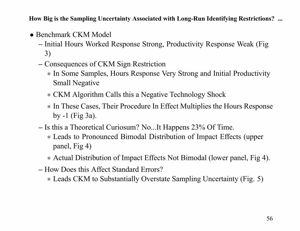
How Big is the Sampling Uncertainty Associated with Long-Run Identifying Restrictions? ...
• Benchmark CKMModel– Initial Hours Worked Response Strong, Productivity Response Weak (Fig
3)
– Consequences of CKM Sign Restriction
In Some Samples, Hours Response Very Strong and Initial Productivity
Small Negative
CKM Algorithm Calls this a Negative Technology Shock
In These Cases, Their Procedure In Effect Multiplies the Hours Response
by -1 (Fig 3a).
– Is this a Theoretical Curiosum? No...It Happens 23% Of Time.
Leads to Pronounced Bimodal Distribution of Impact Effects (upper
panel, Fig 4)
Actual Distribution of Impact Effects Not Bimodal (lower panel, Fig 4).
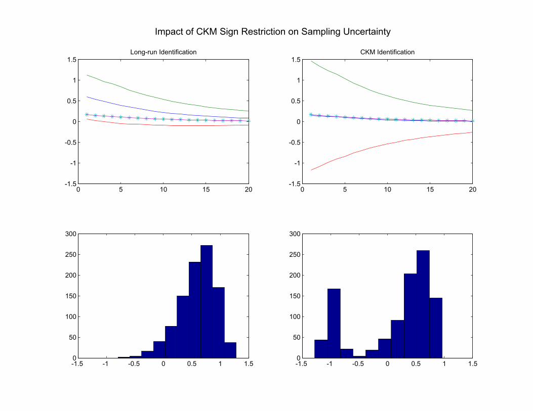
– How Does this Affect Standard Errors?
Leads CKM to Substantially Overstate Sampling Uncertainty (Fig. 5)
56
0 5 10 15 20-1.5
-1
-0.5
0
0.5
1
1.5Long-run Identification
-1.5 -1 -0.5 0 0.5 1 1.50
50
100
150
200
250
300
-1.5 -1 -0.5 0 0.5 1 1.50
50
100
150
200
250
300
Impact of CKM Sign Restriction on Sampling Uncertainty
0 5 10 15 20-1.5
-1
-0.5
0
0.5
1
1.5CKM Identification

Would the Econometrician Be Misled in LargeSamples?
• CKM Say their Benchmark Example Implies ‘Yes’
•We Say ‘No’.– In Practice, Econometrician Applies Diagnostic Tests for Lag Lengths in
VAR
– Four Monte Carlo Simulations of Artificial Data.
Simulate 500 Datasets of length = 1 000; 5 000; 20 000; 50 000
In Each Artificial Data set We Choose Lag Length, as Solution to
min4 45
( )
where ( ) is Akaike criterion.
– Compute Mean Impulse Response Across 500 Data sets (Fig 6)
60
0 1 2 3 4 5 6 7 8 90
0.1
0.2
0.3
0.4
0.5
0.6
0.7T=1000 N =5.2T=5000 N=9.8T=20000 N=14.8T=50000 N=18.5Model

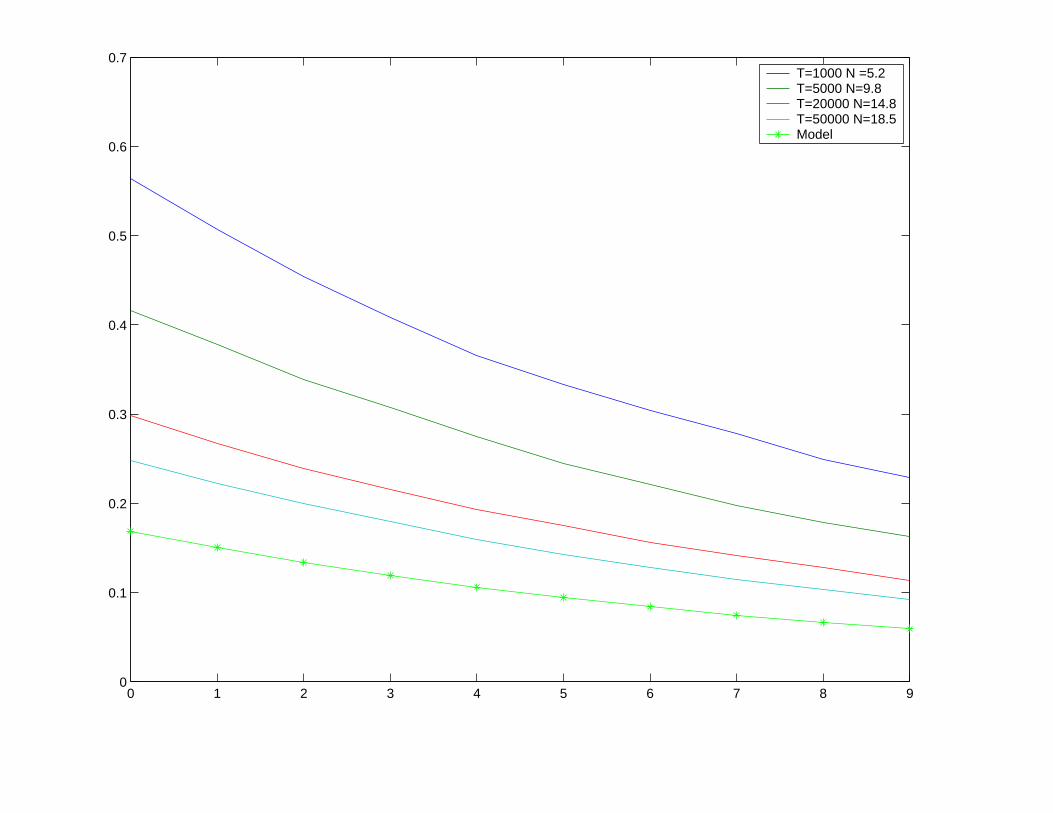
Would the Econometrician Be Misled in LargeSamples?
• CKM Say their Benchmark Example Implies ‘Yes’
•We Say ‘No’.– In Practice, Econometrician Applies Diagnostic Tests for Lag Lengths in
VAR
– Four Monte Carlo Simulations of Artificial Data.
Simulate 500 Datasets of length = 1 000; 5 000; 20 000; 50 000
In Each Artificial Data set We Choose Lag Length, as Solution to
min4 45
( )
where ( ) is Akaike criterion.
– Compute Mean Impulse Response Across 500 Data sets (Fig 6)
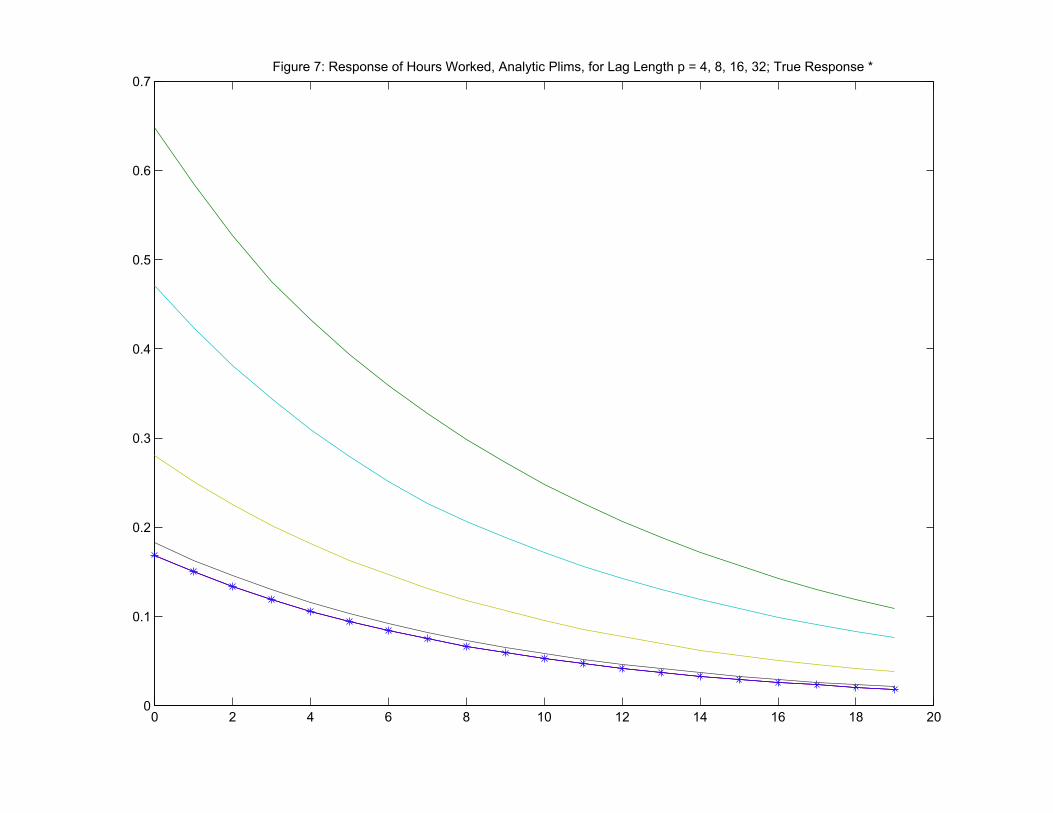
– Key Result: Mean is Converging to Right Solution.
– Unresolved Puzzle: We Get Faster Convergence As Lag Length Increases
(see analytic Plims, Fig 7)
61
0 2 4 6 8 10 12 14 16 18 200
0.1
0.2
0.3
0.4
0.5
0.6
0.7Figure 7: Response of Hours Worked, Analytic Plims, for Lag Length p = 4, 8, 16, 32; True Response *
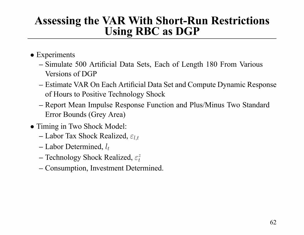
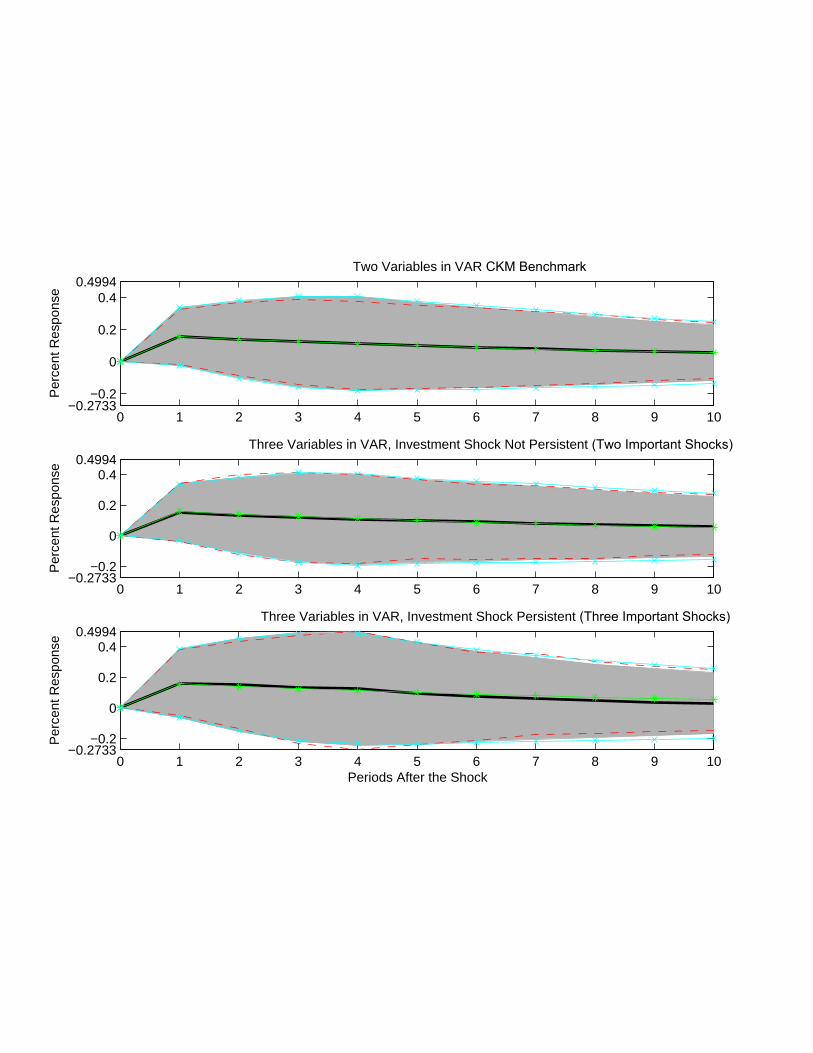
Assessing the VARWith Short-Run RestrictionsUsing RBC as DGP
• Experiments– Simulate 500 Artificial Data Sets, Each of Length 180 From Various
Versions of DGP
– Estimate VAR On Each Artificial Data Set and Compute Dynamic Response
of Hours to Positive Technology Shock
– Report Mean Impulse Response Function and Plus/Minus Two Standard
Error Bounds (Grey Area)
• Timing in Two Shock Model:– Labor Tax Shock Realized,
– Labor Determined,
– Technology Shock Realized,
– Consumption, Investment Determined.
62
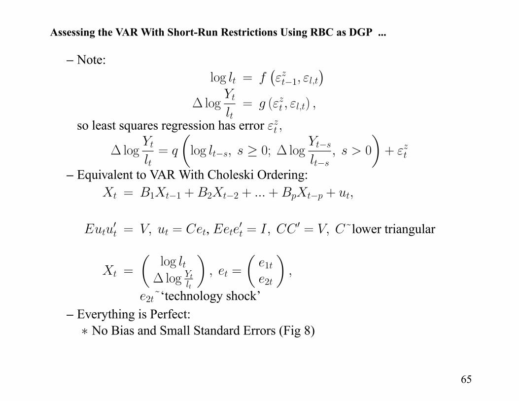
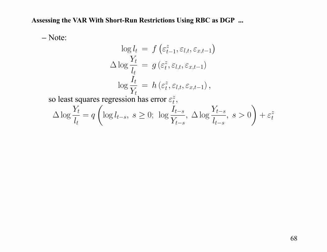
Assessing the VARWith Short-Run Restrictions Using RBC as DGP ...
– Note:
log =¡
1
¢log = ( )
so least squares regression has error
log =
µlog 0; log 0
¶+
– Equivalent to VAR With Choleski Ordering:
= 1 1 + 2 2 + + +
0 = = , 0 = 0 = ˜lower triangular
=
µloglog
¶=
µ1
2
¶2 ˜‘technology shock’
– Everything is Perfect:
No Bias and Small Standard Errors (Fig 8)
65
0 1 2 3 4 5 6 7 8 9 10
−0.2
−0.1
0
0.1
0.2
0.3
0.4P
erce
nt R
espo
nse
Two Variables in VAR Benchmark CKM Model With Timing Restriction
0 1 2 3 4 5 6 7 8 9 10
−0.2
−0.1
0
0.1
0.2
0.3
0.4
Per
cent
Res
pons
e
Three Variables in VAR, Investment Shock Not Persistent (Two Important Shocks)
0 1 2 3 4 5 6 7 8 9 10
−0.2
−0.1
0
0.1
0.2
0.3
0.4
Periods After the Shock
Per
cent
Res
pons
e
Three Variables in VAR, Investment Shock Persistent (Three Important Shocks)

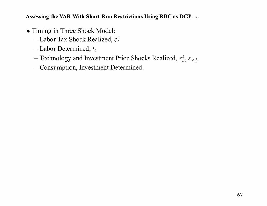
Assessing the VARWith Short-Run Restrictions Using RBC as DGP ...
• Timing in Three Shock Model:– Labor Tax Shock Realized,
– Labor Determined,
– Technology and Investment Price Shocks Realized,
– Consumption, Investment Determined.
67
Assessing the VARWith Short-Run Restrictions Using RBC as DGP ...
– Note:
log =¡
1 1
¢log = ( 1)
log = ( 1)
so least squares regression has error
log =
µlog 0; log log 0
¶+
68

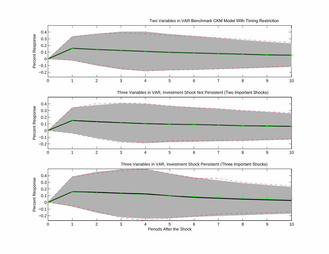
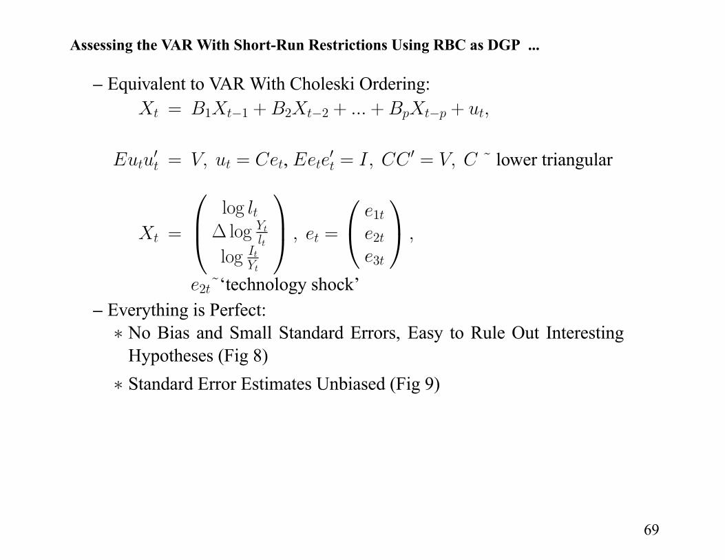
Assessing the VARWith Short-Run Restrictions Using RBC as DGP ...
– Equivalent to VAR With Choleski Ordering:
= 1 1 + 2 2 + + +
0 = = , 0 = 0 = ˜ lower triangular
=
loglog
log=
1
2
3
2 ˜‘technology shock’
– Everything is Perfect:
No Bias and Small Standard Errors, Easy to Rule Out Interesting
Hypotheses (Fig 8)
Standard Error Estimates Unbiased (Fig 9)
69

0 1 2 3 4 5 6 7 8 9 10−0.2733
−0.2
0
0.2
0.40.4994
Per
cent
Res
pons
e
Two Variables in VAR CKM Benchmark
0 1 2 3 4 5 6 7 8 9 10−0.2733
−0.2
0
0.2
0.40.4994
Per
cent
Res
pons
e
Three Variables in VAR, Investment Shock Not Persistent (Two Important Shocks)
0 1 2 3 4 5 6 7 8 9 10−0.2733
−0.2
0
0.2
0.40.4994
Periods After the Shock
Per
cent
Res
pons
e
Three Variables in VAR, Investment Shock Persistent (Three Important Shocks)
Assessing the VARWith Short-Run Restrictions Using RBC as DGP ...
• Timing in Three Shock Model:– Labor Tax Shock Realized,
– Labor Determined,
– Technology and Investment Price Shocks Realized,
– Consumption, Investment Determined.
67

Assessing the VARWith Short-Run Restrictions Using RBC as DGP ...
– Note:
log =¡
1 1
¢log = ( 1)
log = ( 1)
so least squares regression has error
log =
µlog 0; log log 0
¶+
68
Assessing the VARWith Short-Run Restrictions Using RBC as DGP ...
– Equivalent to VAR With Choleski Ordering:
= 1 1 + 2 2 + + +
0 = = , 0 = 0 = ˜ lower triangular
=
loglog
log=
1
2
3
2 ˜‘technology shock’
– Everything is Perfect:
No Bias and Small Standard Errors, Easy to Rule Out Interesting
Hypotheses (Fig 8)
Standard Error Estimates Unbiased (Fig 9)
69
0 1 2 3 4 5 6 7 8 9 10−0.2733
−0.2
0
0.2
0.40.4994
Per
cent
Res
pons
e
Two Variables in VAR CKM Benchmark
0 1 2 3 4 5 6 7 8 9 10−0.2733
−0.2
0
0.2
0.40.4994
Per
cent
Res
pons
e
Three Variables in VAR, Investment Shock Not Persistent (Two Important Shocks)
0 1 2 3 4 5 6 7 8 9 10−0.2733
−0.2
0
0.2
0.40.4994
Periods After the Shock
Per
cent
Res
pons
e
Three Variables in VAR, Investment Shock Persistent (Three Important Shocks)
Key Lessons of the RBCModel Analysis
•With Short Run Exclusion Restrictions, VAR Analysis Highly Accurate
•With Long Run Exclusion Restrictions:– Potential Problems with Large Sampling Uncertainty
– Property of Our Examples: Conditional on Having Enough Variables, the
Analyst Would Know it.
69
Motivation for Additional Analysis
•We Use VAR Impulse Response Functions as part of a Strategy To Formulateand Estimate Monetary DSGE Models
• Basic Strategy: Choose Model Parameters to Make Model-based ImpulseResponses as close as Possible to VAR-based Impulse Responses.
• Problem: How Reliable are VAR-Based Impulse Response Functions?
• Solution: Extend Strategy Pursued Above to Larger DSGE Models, LargerVARs and More Shocks and Variables.
– Run the VAR in Data Generated by the Model.
–We Look at this in ACEL.
70
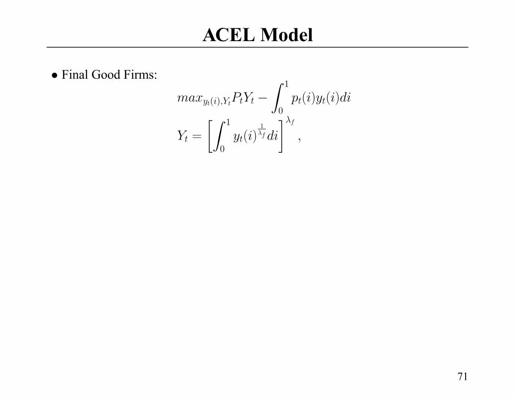
ACELModel
• Final Good Firms:
( )
Z 1
0
( ) ( )
=
Z 1
0
( )1
¸
71
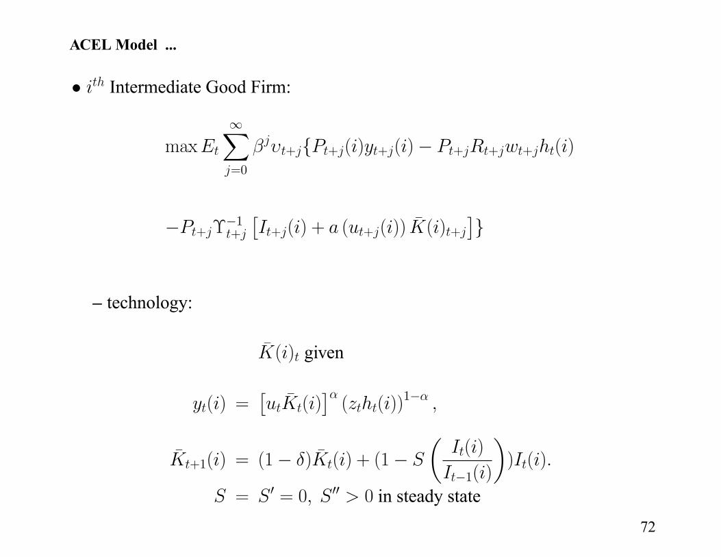
ACEL Model ...
• Intermediate Good Firm:
maxX=0
+ { + ( ) + ( ) + + + ( )
+1+
£+ ( ) + ( + ( )) ¯ ( ) +
¤}
– technology:
¯ ( ) given
( ) =£
¯ ( )¤( ( ))1
¯+1( ) = (1 ) ¯ ( ) + (1
µ( )
1( )
¶) ( )
= 0 = 0 00 0 in steady state
72
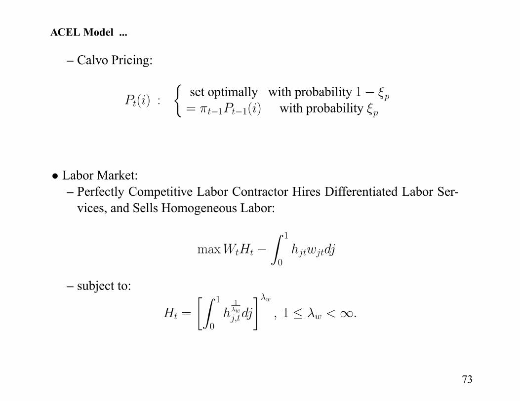
ACEL Model ...
– Calvo Pricing:
( ) :
½set optimally with probability 1= 1 1( ) with probability
• Labor Market:– Perfectly Competitive Labor Contractor Hires Differentiated Labor Ser-
vices, and Sells Homogeneous Labor:
max
Z 1
0
– subject to:
=
Z 1
0
1
¸1
73
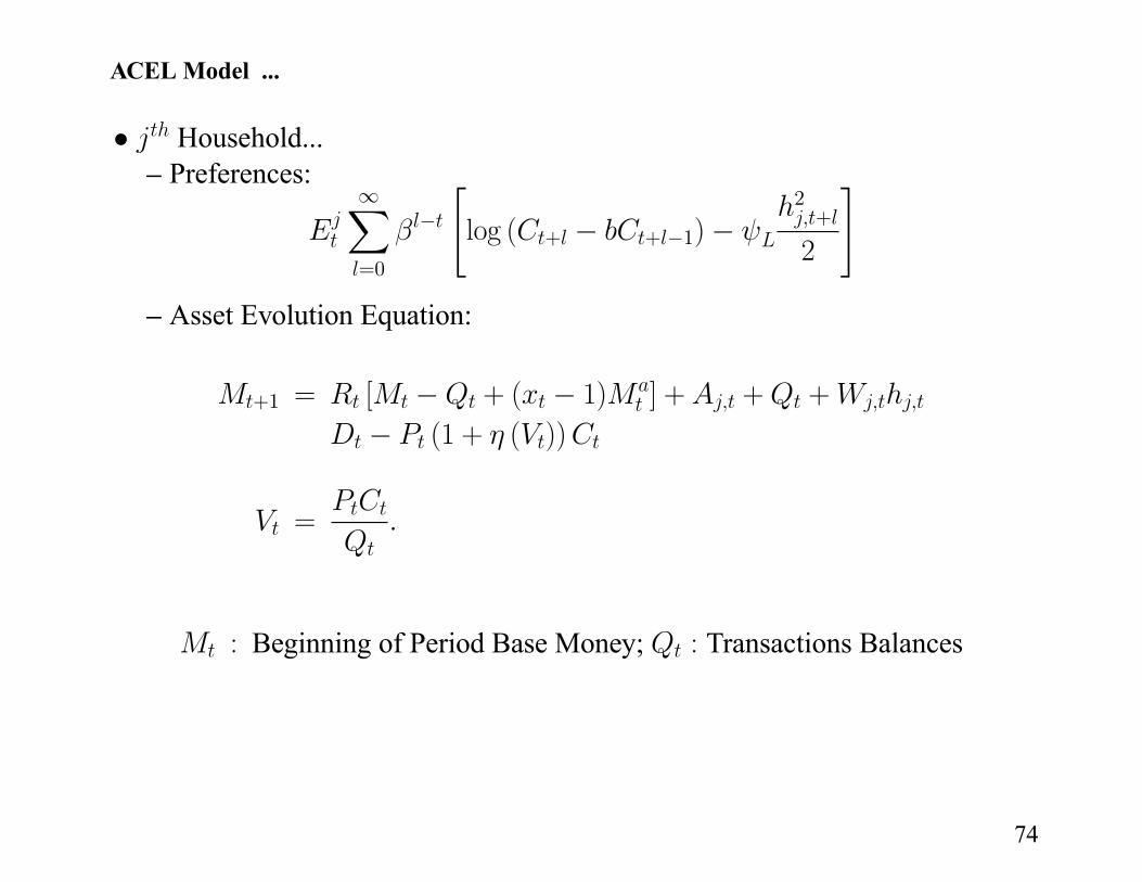
ACEL Model ...
• Household...
– Preferences: X=0
"log ( + + 1)
2+
2
#
– Asset Evolution Equation:
+1 = [ + ( 1) ] + + +
(1 + ( ))
=
: Beginning of Period Base Money; : Transactions Balances
74
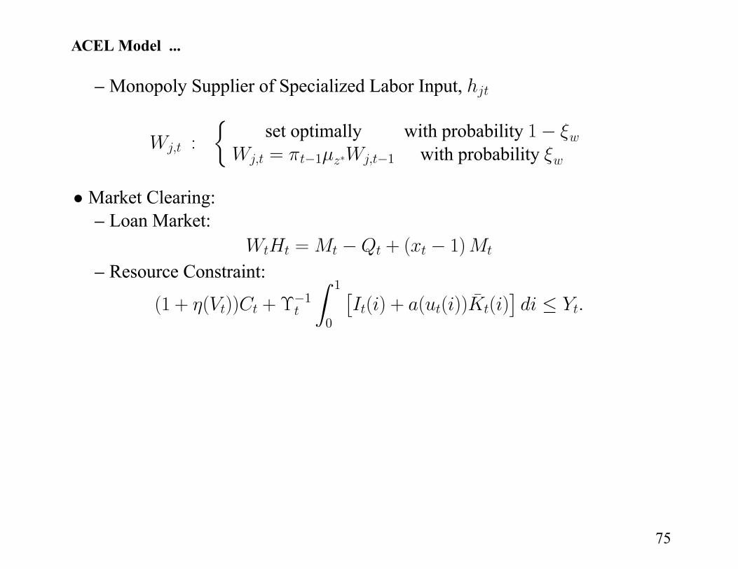
ACEL Model ...
– Monopoly Supplier of Specialized Labor Input,
:
½set optimally with probability 1= 1 1 with probability
• Market Clearing:– Loan Market:
= + ( 1)
– Resource Constraint:
(1 + ( )) + 1
Z 1
0
£( ) + ( ( )) ¯ ( )
¤
75
ACEL Model ...
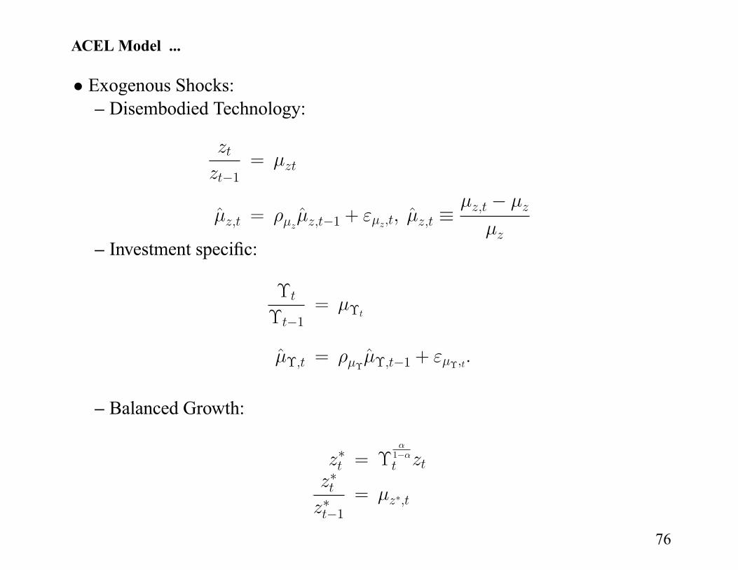
• Exogenous Shocks:– Disembodied Technology:
1=
ˆ = ˆ 1 + ˆ
– Investment specific:
1=
ˆ = ˆ 1 +
– Balanced Growth:
= 1
1
=
76
ACEL Model ...
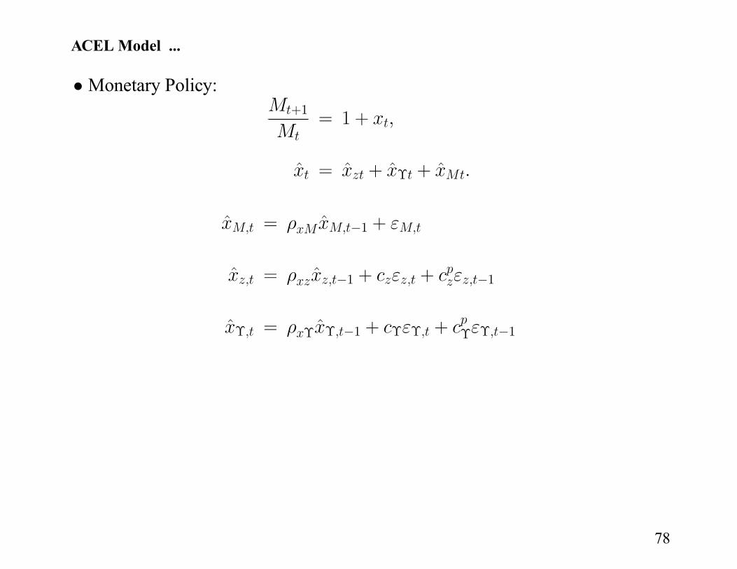
• Monetary Policy:+1= 1 +
ˆ = ˆ + ˆ + ˆ
ˆ = ˆ 1 +
ˆ = ˆ 1 + + 1
ˆ = ˆ 1 + + 1
78
ACEL Model ...
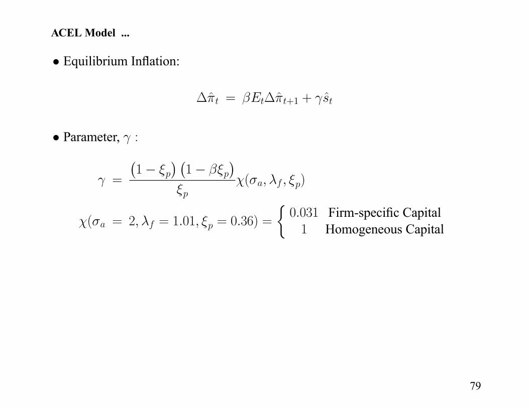
• Equilibrium Inflation:
ˆ = ˆ +1 + ˆ
• Parameter, :
=
¡1
¢ ¡1
¢( )
( = 2 = 1 01 = 0 36) =
½0 031 Firm-specific Capital
1 Homogeneous Capital
79
QQ0
P0
P1
P2
MC0
MC1
MC0,f
MC1,f
A
B
B

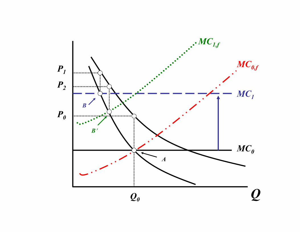
ACEL Model ...
• Intuition About Importance of Firm Specificity of Capital– A Firm Contemplates Raising Price
– This Implies Output Falls
– Marginal Cost Falls
– Incentive to Raise Price Falls
• Effect Quantitatively Important When:– Demand Elastic
– Marginal Cost Steep
80
Estimating Parameters in the Model
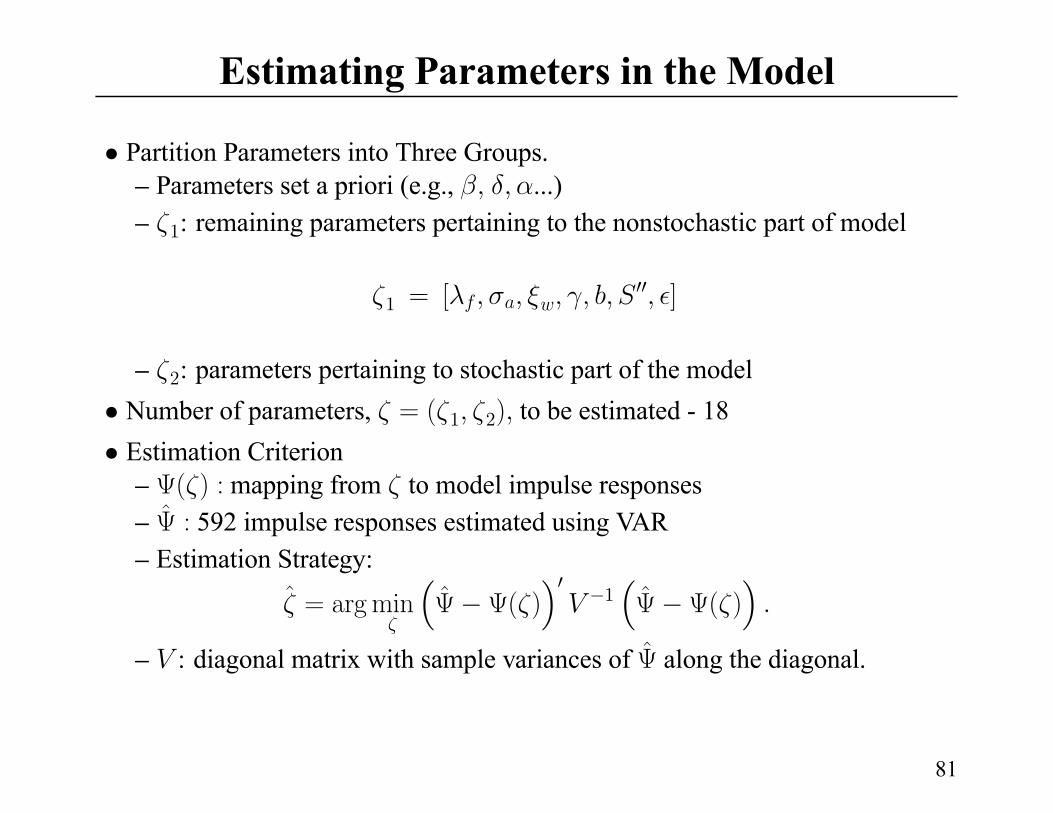
• Partition Parameters into Three Groups.– Parameters set a priori (e.g., ...)
– 1: remaining parameters pertaining to the nonstochastic part of model
1 = [ 00 ]
– 2: parameters pertaining to stochastic part of the model
• Number of parameters, = ( 1 2) to be estimated - 18
• Estimation Criterion– ( ) : mapping from to model impulse responses
– ˆ : 592 impulse responses estimated using VAR
– Estimation Strategy:
ˆ = argmin³ˆ ( )
´01³ˆ ( )
´– : diagonal matrix with sample variances of ˆ along the diagonal.
81
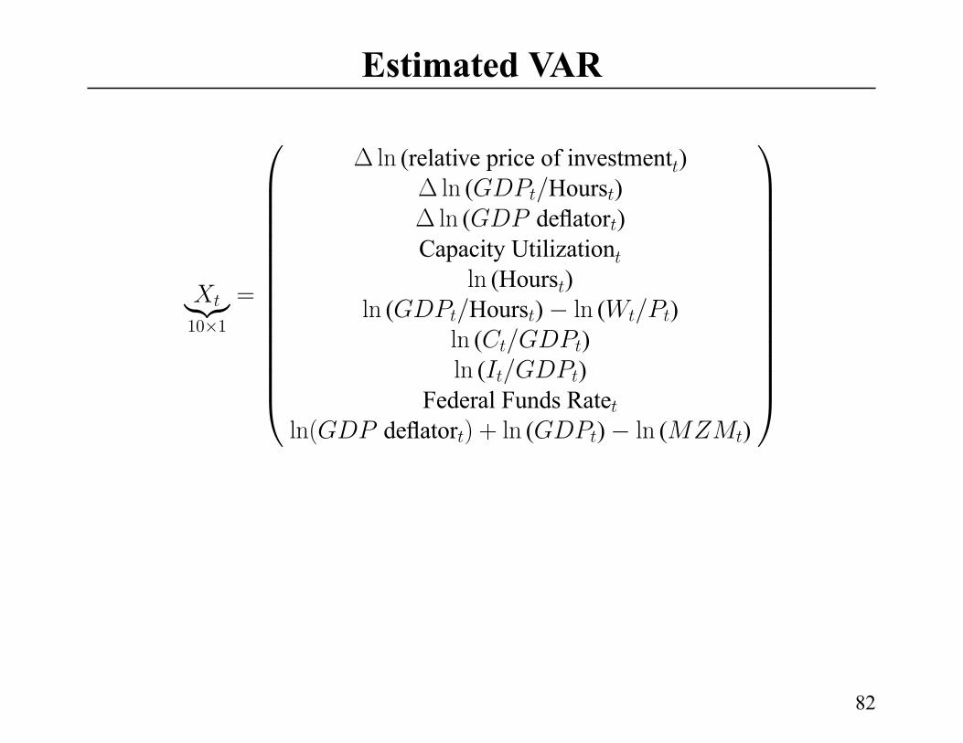
Estimated VAR
|{z}10×1
=
ln (relative price of investment )ln ( Hours )
ln ( deflator )
Capacity Utilization
ln (Hours )ln ( Hours ) ln ( )
ln ( )
ln ( )
Federal Funds Rate
ln( deflator ) + ln ( ) ln ( )
82
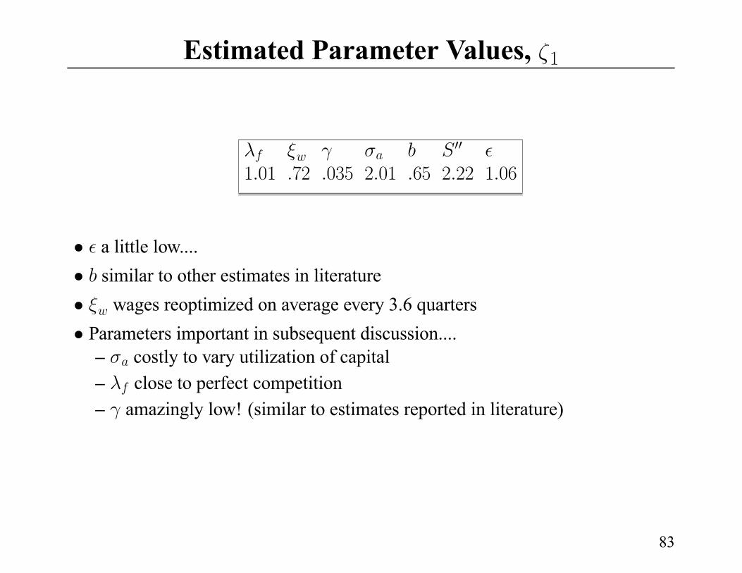
Estimated Parameter Values, 1
00
1 01 72 035 2 01 65 2 22 1 06
• a little low....
• similar to other estimates in literature
• wages reoptimized on average every 3.6 quarters
• Parameters important in subsequent discussion....– costly to vary utilization of capital
– close to perfect competition
– amazingly low! (similar to estimates reported in literature)
83
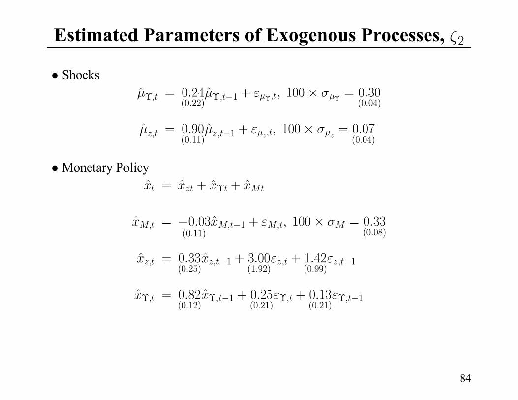
Estimated Parameters of Exogenous Processes, 2
• Shocks
ˆ = 0 24(0 22)
ˆ 1 + 100× = 0 30(0 04)
ˆ = 0 90(0 11)
ˆ 1 + 100× = 0 07(0 04)
• Monetary Policy
ˆ = ˆ + ˆ + ˆ
ˆ = 0 03(0 11)
ˆ 1 + 100× = 0 33(0 08)
ˆ = 0 33(0 25)
ˆ 1 + 3 00(1 92)
+ 1 42(0 99)
1
ˆ = 0 82(0 12)
ˆ 1 + 0 25(0 21)
+ 0 13(0 21)
1
84
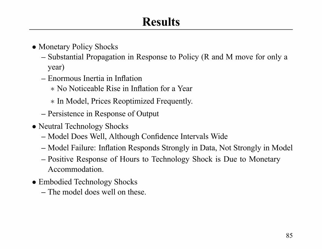
Results
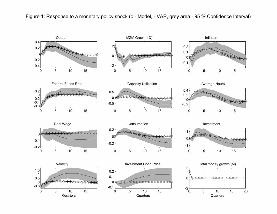
• Monetary Policy Shocks– Substantial Propagation in Response to Policy (R and M move for only a
year)
– Enormous Inertia in Inflation
No Noticeable Rise in Inflation for a Year
In Model, Prices Reoptimized Frequently.
– Persistence in Response of Output
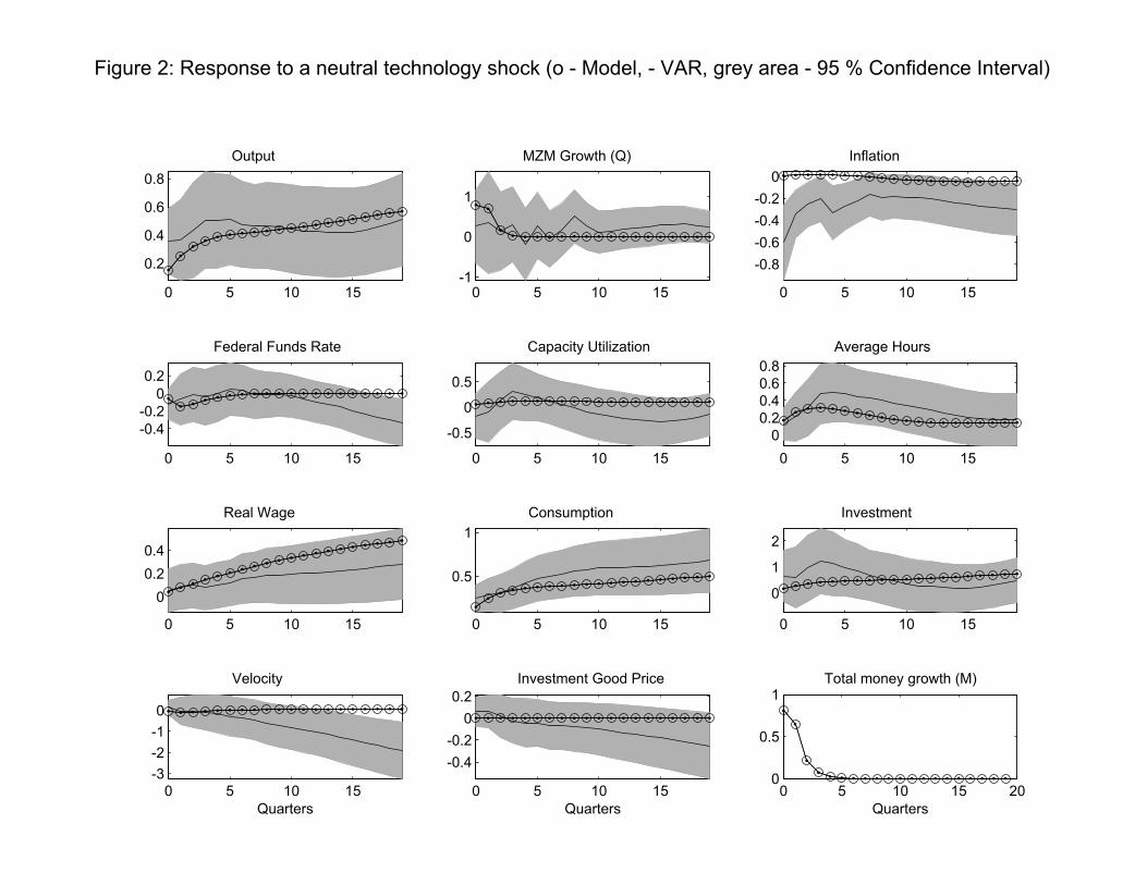
• Neutral Technology Shocks– Model Does Well, Although Confidence Intervals Wide
– Model Failure: Inflation Responds Strongly in Data, Not Strongly in Model
– Positive Response of Hours to Technology Shock is Due to Monetary
Accommodation.
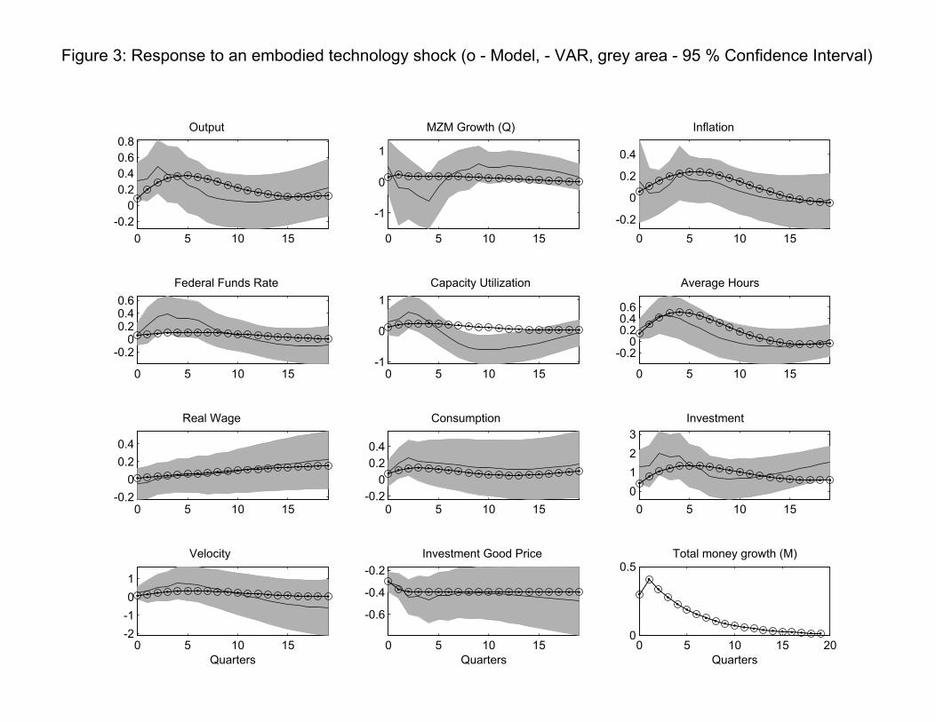
• Embodied Technology Shocks– The model does well on these.
85
0 5 10 15
-0.4
-0.2
0
0.2
0.4
Output
0 5 10 15
-2
0
2
MZM Growth (Q)
0 5 10 15
-0.1
0
0.1
0.2
Inflation
0 5 10 15
-0.6-0.4-0.2
00.2
Federal Funds Rate
0 5 10 15
-0.5
0
0.5
Capacity Utilization
0 5 10 15
-0.2
0
0.2
0.4
Average Hours
0 5 10 15-0.2
-0.1
0
Real Wage
0 5 10 15
-0.2
0
0.2
Consumption
0 5 10 15
-1
0
1
Investment
0 5 10 15
-0.50
0.51
1.5
Velocity
Quarters
0 5 10 15-0.1
0
0.1
0.2
Investment Good Price
Quarters
Figure 1: Response to a monetary policy shock (o - Model, - VAR, grey area - 95 % Confidence Interval)
0 5 10 15 20-2
0
2Total money growth (M)
Quarters
0 5 10 15
0.2
0.4
0.6
0.8
Output
0 5 10 15-1
0
1
MZM Growth (Q)
0 5 10 15
-0.8
-0.6
-0.4
-0.2
0
Inflation
0 5 10 15
-0.4
-0.2
0
0.2
Federal Funds Rate
0 5 10 15
-0.5
0
0.5
Capacity Utilization
0 5 10 15
0
0.2
0.4
0.6
0.8
Average Hours
0 5 10 15
0
0.2
0.4
Real Wage
0 5 10 15
0.5
1
Consumption
0 5 10 15
0
1
2
Investment
0 5 10 15
-3
-2
-1
0
Velocity
Quarters
0 5 10 15
-0.4
-0.2
0
0.2
Investment Good Price
Quarters
Figure 2: Response to a neutral technology shock (o - Model, - VAR, grey area - 95 % Confidence Interval)
0 5 10 15 200
0.5
1Total money growth (M)
Quarters
0 5 10 15
-0.2
0
0.2
0.4
0.6
0.8
Output
0 5 10 15
-1
0
1
MZM Growth (Q)
0 5 10 15
-0.2
0
0.2
0.4
Inflation
0 5 10 15
-0.20
0.20.40.6
Federal Funds Rate
0 5 10 15-1
0
1
Capacity Utilization
0 5 10 15
-0.20
0.20.40.6
Average Hours
0 5 10 15-0.2
0
0.2
0.4
Real Wage
0 5 10 15-0.2
0
0.2
0.4
Consumption
0 5 10 15
0
1
2
3
Investment
0 5 10 15-2
-1
0
1
Velocity
Quarters
0 5 10 15
-0.6
-0.4
-0.2
Investment Good Price
Quarters
Figure 3: Response to an embodied technology shock (o - Model, - VAR, grey area - 95 % Confidence Interval)
0 5 10 15 200
0.5Total money growth (M)
Quarters
Question
•We fit Impulse Responses Reasonably Well, But Do We Have Any Reason toTrust Them?
• Obvious Experiment:–What if the Estimated Model were literally true, How Well Would Our
Procedure Work?
–We Plan to Study the Sampling Distribution of our Parameter Estimator
– For Now, We Repeated the RBC analysis Described Above.
86
Plan
• Basic Idea: Generate Data from DSGE Model and Fit VARs in Artificial Data
• Problem:– DSGE Model Has Too Few Shocks
– Empirical Procedure Recognizes We’re Short on Shocks and Offers a
Natural Solution
87
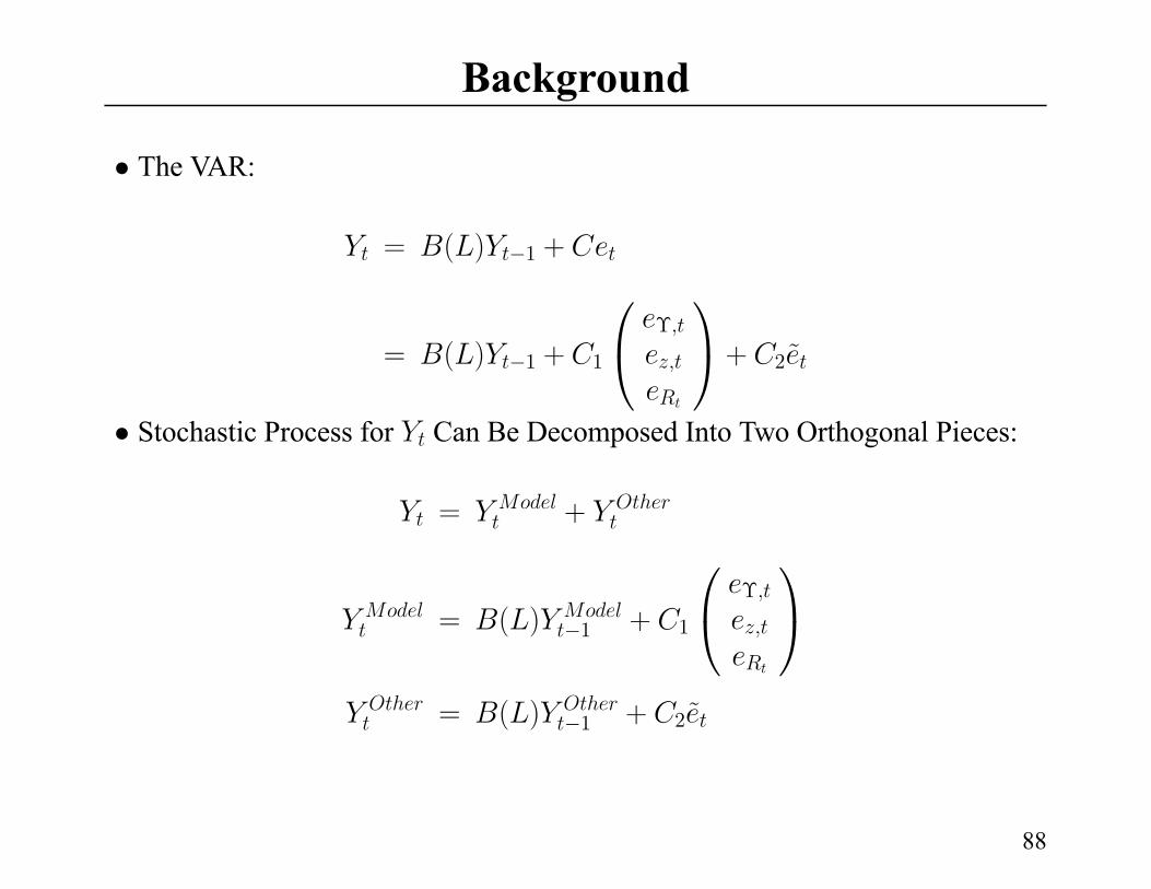
Background
• The VAR:
= ( ) 1 +
= ( ) 1 + 1 + 2˜
• Stochastic Process for Can Be Decomposed Into Two Orthogonal Pieces:
= +
= ( ) 1 + 1
= ( ) 1 + 2˜
88
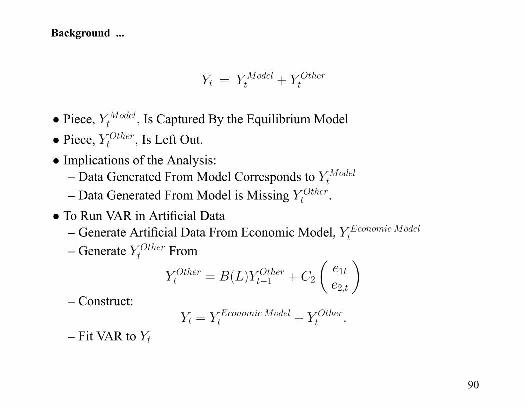
Background ...
= +
• Piece, Is Captured By the Equilibrium Model
• Piece, Is Left Out.
• Implications of the Analysis:– Data Generated From Model Corresponds to
– Data Generated From Model is Missing .
• To Run VAR in Artificial Data– Generate Artificial Data From Economic Model,
– Generate From
= ( ) 1 + 2
µ1
2
¶– Construct:
= +
– Fit VAR to
90
Experiment
• Generate Artificial Data– Extremely Long Data Set to Get Plim (20,000 Observations)
– Many Data Sets of Length 170 Each
• Feed Each Data Set to Same VAR Fit to US Data
• Compute Impulse Response Functions– Dotted Lines: Small Sample Means
– Dashed Lines: Plims
91
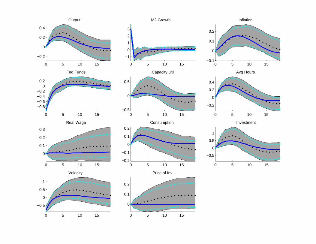
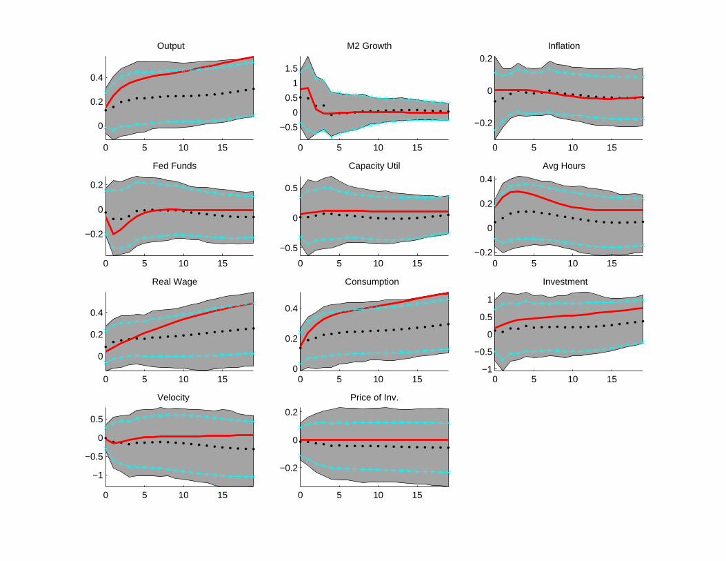
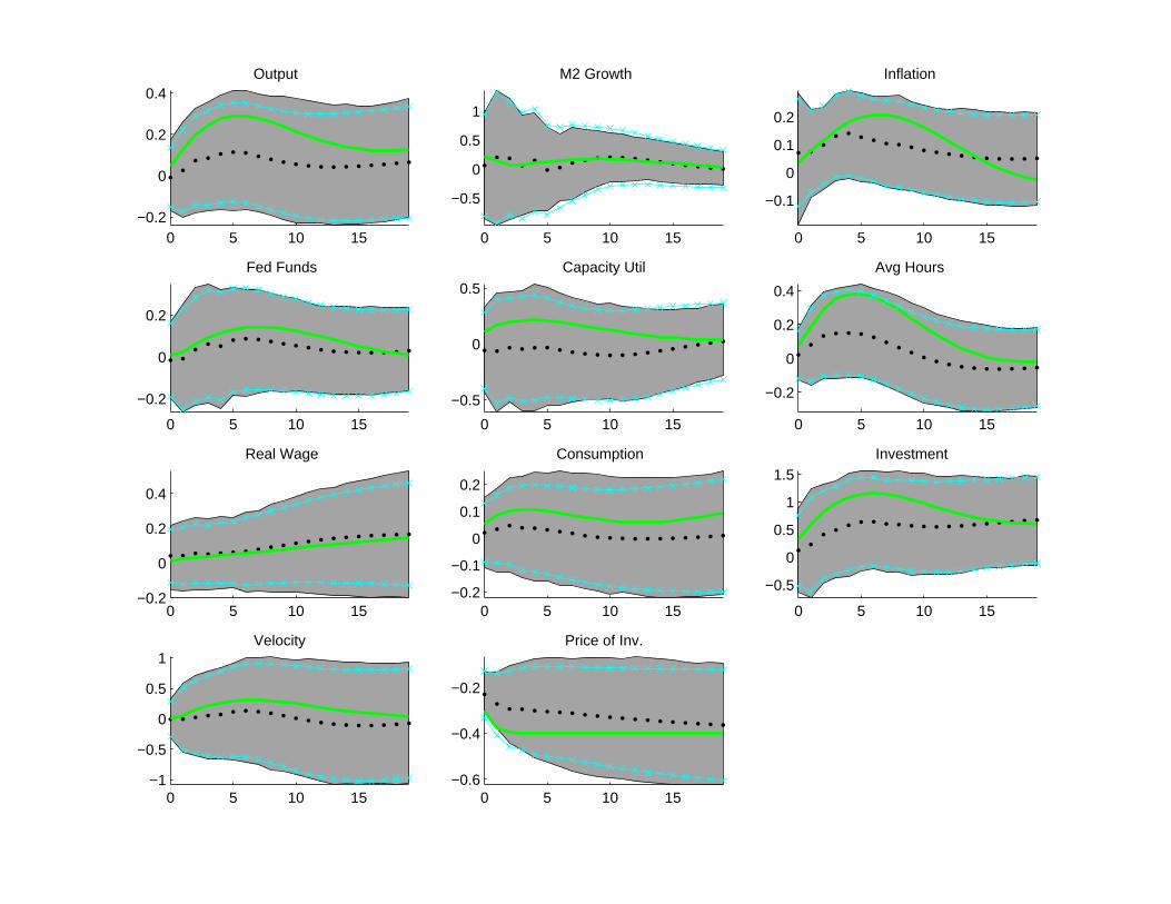
Findings
• Contents of Figures– x’s - mean impulse response, plus/minus two times mean standard deviation
estimated by econometrician
– Solid line: truth
– Dotted line: small sample mean from VAR
– Gray area: mean impulse response, plus/minus two times actual standard
deviation of impulse response.
92
Findings ...
• Monetary Policy Shock– Bias Reasonably Small
– Estimator of Uncertainty Acceptable (Though Some Bias Down)
• Neutral Technology Shock
– Overall, Bias Small, But Output, Investment and Real Wage Biased Down– Notable Finding: Inflation Response Rules Out Estimated VAR Inflation
Response
VAR Confidence Interval: -0.22 to -0.80 percent
Evidence Against ACEL Model.
Evidence of Potential Power of Long-Run Restrictions.
• Embodied Technology Shock– Performs Reasonably, Overall
93
0 5 10 15
−0.2
0
0.2
0.4
Output
0 5 10 15
−1
0
1
2
3
M2 Growth
0 5 10 15−0.1
0
0.1
0.2
Inflation
0 5 10 15
−0.8−0.6−0.4−0.2
00.2
Fed Funds
0 5 10 15−0.5
0
0.5
Capacity Util
0 5 10 15
−0.2
0
0.2
0.4
Avg Hours
0 5 10 15
0
0.1
0.2
0.3
Real Wage
0 5 10 15−0.2
−0.1
0
0.1
0.2
Consumption
0 5 10 15
−0.5
0
0.5
1
Investment
0 5 10 15
−0.5
0
0.5
1
Velocity
0 5 10 15
0
0.1
0.2
Price of Inv.
0 5 10 15
0
0.2
0.4
Output
0 5 10 15
−0.5
0
0.5
1
1.5
M2 Growth
0 5 10 15
−0.2
0
0.2Inflation
0 5 10 15
−0.2
0
0.2
Fed Funds
0 5 10 15
−0.5
0
0.5
Capacity Util
0 5 10 15−0.2
0
0.2
0.4
Avg Hours
0 5 10 15
0
0.2
0.4
Real Wage
0 5 10 150
0.2
0.4
Consumption
0 5 10 15−1
−0.5
0
0.5
1
Investment
0 5 10 15
−1
−0.5
0
0.5
Velocity
0 5 10 15
−0.2
0
0.2
Price of Inv.
0 5 10 15−0.2
0
0.2
0.4Output
0 5 10 15
−0.5
0
0.5
1
M2 Growth
0 5 10 15
−0.1
0
0.1
0.2
Inflation
0 5 10 15
−0.2
0
0.2
Fed Funds
0 5 10 15
−0.5
0
0.5
Capacity Util
0 5 10 15
−0.2
0
0.2
0.4
Avg Hours
0 5 10 15−0.2
0
0.2
0.4
Real Wage
0 5 10 15−0.2
−0.1
0
0.1
0.2
Consumption
0 5 10 15
−0.5
0
0.5
1
1.5Investment
0 5 10 15−1
−0.5
0
0.5
1Velocity
0 5 10 15−0.6
−0.4
−0.2
Price of Inv.
Conclusion
• VARs With Long-Run Restrictions:– Can Be Imprecise, But Standard Errors Let You Know
– Can Have Power
See Prescott RBC Model
See Evidence Against ACEL Model
• VARs With Short-Run Restrictions:– Appear to Be Precise
• Simulations Like the Ones Done Here (following Erceg-Guerrieri-Gust, andCKM) Important as Ultimate Guard Against Being Misled
– However, in Models Which Do Not Specify All Shocks, Must Use
Something Like ACEL Procedure to Add Estimate of Other Shocks.
96