Voltage regulation of unbalanced distribution network with

University of Northern Iowa University of Northern Iowa

UNI ScholarWorks UNI ScholarWorks

Dissertations and Theses @ UNI Student Work

2018

Voltage regulation of unbalanced distribution network with Voltage regulation of unbalanced distribution network with

distributed generators through genetic algorithm distributed generators through genetic algorithm

Islam Ali University of Northern Iowa

Let us know how access to this document benefits you

Copyright ©2018 Islam Ali

Follow this and additional works at: https://scholarworks.uni.edu/etd

Part of the Electrical and Electronics Commons

Recommended Citation Recommended Citation Ali, Islam, "Voltage regulation of unbalanced distribution network with distributed generators through genetic algorithm" (2018). Dissertations and Theses @ UNI. 678. https://scholarworks.uni.edu/etd/678

This Open Access Dissertation is brought to you for free and open access by the Student Work at UNI ScholarWorks. It has been accepted for inclusion in Dissertations and Theses @ UNI by an authorized administrator of UNI ScholarWorks. For more information, please contact [email protected].

https://scholarworks.uni.edu/

https://scholarworks.uni.edu/etd

https://scholarworks.uni.edu/sw_gc

https://scholarworks.uni.edu/feedback_form.html

https://scholarworks.uni.edu/etd?utm_source=scholarworks.uni.edu%2Fetd%2F678&utm_medium=PDF&utm_campaign=PDFCoverPages

http://network.bepress.com/hgg/discipline/270?utm_source=scholarworks.uni.edu%2Fetd%2F678&utm_medium=PDF&utm_campaign=PDFCoverPages

https://scholarworks.uni.edu/etd/678?utm_source=scholarworks.uni.edu%2Fetd%2F678&utm_medium=PDF&utm_campaign=PDFCoverPages

mailto:[email protected]

Copyright by

ISLAM ALI

2018

All Rights Reserved

VOLTAGE REGULATION OF UNBALANCED DISTRIBUTION NETWORK WITH

DISTRIBUTED GENERATORS THROUGH GENETIC ALGORITHM

An Abstract of a Dissertation

Submitted

in Partial Fulfillment

of the Requirements for the Degree

Doctor of Industrial Technology

Approved: ____________________________________ Dr. Hong Nie, Committee Chair ____________________________________

Dr. Patrick Pease Interim Dean of the Graduate College

Islam Ali

University of Northern Iowa

July, 2018

ABSTRACT

Energy demand has rapidly increased since the manufacturing revolution in the

19th century. One of the higher energy demands is electricity. The great majority of

devices in the manufacturing field run on electricity. The vertically integrated grid

paradigm has to be changed to supply the increase in the electrical demand residentially

and commercially. Distributed generators (DG) such as Photovoltic (PV) is used to

supply the increase in the electrical demand. Photovoltaic (PV) is one of the fast growing

distributed generators (DG) as a renewable energy source. However, installing many PV

systems to the distribution system can cause power quality problems such as over

voltage. This would be more concern in an unbalanced electrical distribution network

where nowadays most of the PV systems are connected. PV system should coordinate

with other DGs and already existing voltage regulators such as on load tap changer

(OLTC) on voltage regulation so that they can support the electrical grid without adding

voltage problems. This dissertation focuses on voltage regulation of unbalanced

distribution system through the utilization of PV reactive power feature by minimizing

the system losses using genetic algorithm. The proposed method provides a single phase

controlled PV system that regulates each phase voltage individually and focuses in

maintaining the voltage for each phase within a certain limit. In addition, this study

proposes a single-phase OLTC control by changing the tap position individually using

loss minimization. The proposed algorithm is implemented in Matlab and Simulink.

Results show that the PV reactive power can be utilized to control the system voltage as

well as to minimize the traditional voltage regulator operations.

VOLTAGE REGULATION OF UNBALANCED DISTRIBUTION NETWORK WITH

DISTRIBUTED GENERATORS THROUGH GENETIC ALGORITHM

A Dissertation

Submitted

in Partial Fulfillment

of the Requirements for the Degree

Doctor of Industrial Technology

Approved: ___________________________________ Dr. Hong Nie, Committee Chair ___________________________________ Dr. Sadik Kucuksari, Co-Chair ___________________________________ Dr. Shahram VarzaVand, Committee Member ___________________________________ Dr. Mark Ecker, Committee Member ___________________________________ Dr. Paul Shand, Committee Member

Islam Ali

University of Northern Iowa

July, 2018

ii

ACKNOWLEDGEMENT

I would like to thank the University of Northern Iowa (UNI) for providing me this

opportunity to study and do this research. I would like to thank Dr. Hong Nie, the

chairman of my committee, for his support throughout all of these the years, since I

started my Masters degree in 2010. I would like to thank Dr. Sadik Kucuksari, my co-

chairman and mentor, for his support and guidance. He spent a great deal of his time

coaching and guiding me throughout this research. His experience in research and writing

technical papers taught me more than I could have imagined. These skills will stay with

me for the rest of my career. I would like to thank Dr. VarzaVand for his support

throughout my degree. I took several classes with Dr. VarzaVand and I learned a great

deal from him inside and outside of academia. I would like to thank Dr. Mark Ecker and

Dr. Paul Shand for their valuable input. Both of their contributions were imperative to the

successful completion of this dissertation. I want to thank my committee members for

their unyielding support.

I would like to thank all of my teachers who helped me to learn and reach my

goals since I was young. I would like to thank everyone who gave me advice and

supported and encouraged me. I would not have been here without all of this generous

support.

I would like to thank my mother for all the sacrifices she made to raise me as a

widowed mother. Even with all of the distance between us, she always supported and

encouraged me. I would like to thank my late father for instilling the love of engineering

and science in me at an early age. I did not spend much time with him, but the time we

iii

spent together before his passing had a great impact on me. I hope he is proud of me. I

want to thank my wife for her support and sacrifices during my study. You did a lot for

me and it would not be possible without your support. You took care of many

responsibilities, so I can focus on my study. I want to thank my daughters for their

support and I hope I can be a good example to them. Watching them growing and smiling

and playing encouraged me to do my best. I would like to thank my brothers for their

support and guidance since I was young. I would extend my sincere gratitude to Dr.

Fahmy and my aunt for their support and patience since I came to the United States. They

always encouraged me and shared their experiences with me which served as great

motivation. I would like to thank my uncle, Dr. Ahmed Metwali, and his wife, Dr.

Nervana Metwali who stood by my family and me during a tense time. They were with

my wife and kids at all the times I could not be. I would like to thank my family and

friends back in Egypt. Thanks for the constant stream of encouragement. I would not

make it without all of their support.

I remember sitting in Cairo International airport waiting for my flight to the

United States. I did not know what I was doing and was contemplating whether I would

succeed. In the eight years I have been here, I have learned so much about academia and

in life. I have so many great memories that will forever be etched into my story. I would

like to thank everyone who was part of this journey.

I hope this dissertation will be a good example for anyone believes that his/her

dream is too far to be achieved. I, too, thought that was true one day.

iv

TABLE OF CONTENTS

PAGE 34TLIST OF TABLES34T ..................................................................................................... viiviiii

34TLIST OF FIGURES34T ..............................................................................................viiviiiviiii

34TLIST OF EQUATIONS34T ......................................................................................................x

34TCHAPTER 1. INTRODUCTION34T .....................................................................................11

34TBackground34T .................................................................................................................... 2

34TStatement of Problem34T ..................................................................................................... 4

34TPurpose of the Study34T ...................................................................................................... 4

34TNeed for the Study34T.......................................................................................................... 5

34TAssumptions of the Study34T .............................................................................................. 6

34TResearch Question34T .......................................................................................................... 6

34TLimitations of the Study34T ................................................................................................. 6

34TCHAPTER 2. LITERATURE REVIEW34T ............................................................................7

34TPV34T ................................................................................................................................... 7 34TInverters34T ........................................................................................................................ 11

34T1. Centralized inverters34T ............................................................................................. 12

2. String Inverters and AC Modules ........................................................................... 12

3. Multi string inverters .............................................................................................. 22

34T4. AC-Module Technology34T ....................................................................................... 22

34TReactive Power Control34T ............................................................................................... 22

34TGenetic Algorithm34T ........................................................................................................ 23

v

34TOLTC34T ........................................................................................................................... 28

34TSummary34T ...................................................................................................................... 30

34TScope of the Research 34T ................................................................................................. 32

34TCHAPTER 3. METHODOLOGY34T .................................... Error! Bookmark not defined.

34TUnbalanced Distribution System Voltage34T .................................................................... 35

34TOLTC and PV Model Modifications34T ............................................................................ 37

34TCoordinated Voltage Control through Loss Minimization34T .......................................... 39

34TTest Cases34T ..................................................................................................................... 44

34TCHAPTER 4. RESULTS AND DISCUSSIONS34T .............................................................46

34TCase 134T ........................................................................................................................... 46 34TCase 234T ........................................................................................................................... 51

34TCase 334T ........................................................................................................................... 55

34TCase 434T ........................................................................................................................... 60

34TSummary34T ...................................................................................................................... 63

34TCHAPTER 5. CONCLUSION AND FUTURE RECOMMENDATIONS34T ...................654

34TConclusion34T .................................................................................................................... 64

34THow can coordinated control improve the voltage profile of an unbalanced distribution system?34T ......................................................................................................................... 64 34TWould PV reduce the OLTC operation?34T ...................................................................... 65

34THow can OLTC and PV system control unbalanced distribution system voltage?34T ..... 65

34THow can GA optimize the distribution system to reduce the electrical losses?34T ........... 65

34TFuture Recommendation34T ............................................................................................ 676

34TREFERENCES34T .................................................................................................................67

vi

34TAPPENDIX.34T......................................................................................................................70

34TNAPS 201834T ................................................................................................................... 70

34TCASE 1 MAIN M FILE34T ............................................................................................... 76

34TCASE 1 PI PARAMETERS M FILE34T ........................................................................... 76

34TCASE 234T ......................................................................................................................... 77



34TCASE 334T ......................................................................................................................... 79



34TCASE 434T ......................................................................................................................... 81



vii

LIST OF TABLES

TABLE PAGE

34TU 1 Optimization parameters (Case 1)U34T ...................................................................... 50

34TU 2 Optimization parameters (Case 2)U34T ...................................................................... 53

34TU 3 Buses voltage (Case 2)U34T ....................................................................................... 54


34TU 5 The optimized parameters (Case 3)U34T .................................................................... 59


viii

LIST OF FIGURES

FIGURE PAGE

1 One line diagram for the electrical distribution system that includes DG at the load side ................................................................................................................. 2

34T2 34TI-V curve with different irradiances ...................................................................... 8

34T3 34TPower-Voltage curve with different irradiances .................................................. 9

34T4 34TI-V curve with different temperature .................................................................. 10

34T5 34TP-V curve with different temperature ................................................................. 10

34T6 34TSensitivity method ............................................................................................... 14

34T7 34TE.ON code during faults ...................................................................................... 15

34T8 34TControl algorithm for the voltage regulation ....... Error! Bookmark not defined.

34T9 34TQ controller algorithm ......................................................................................... 18

34T10 34TFlow chart for the optimization algorithm .......................................................... 21

34T11 34TSingle line diagram for a distribution system ..................................................... 22

34T12 34TReactor and resistor principle ............................................................................. 30

34T13 34TBase case without voltage regulation (Bus 632) ................................................. 35

34T14 34TBase case without PV system (Bus 632) ............................................................. 36

34T15 34TModified IEEE 13 bus ......................................................................................... 37

34T16 34TOLTC windings configuration ............................................................................ 38

34T17 34TAlgorithm flow chart ........................................................................................... 44

34T18 34TCase 1 test system ............................................................................................... 47

34T19 34TCircuit simulation in Simulink ............................................................................ 49

34T20 34TVR3R voltage ........................................................................................................... 51

ix

34T21 34TVoltages at buses 632 & 675 (Case 2) ................................................................ 52

34T22 34TReactive power injected from PV system (Case 2) ............................................. 53

34T23 34TVoltages at buses 632 & 675 (Case 3) ................ Error! Bookmark not defined.

34T24 34TReactive power injected from PV system (Case 3) ............ Error! Bookmark not

defined.

34T25 34TVoltages at buses 632 & 675 (Case 4) ................................................................ 60

34T26 34TReactive power injected from PV system (Case 4) ............................................. 61

x

LIST OF EQUATIONS

EQUATION PAGE

1 Active Power ............................................................................................... 17

2 Reactive Power ........................................................................................... 17

3 Power losses ................................................................................................ 21

4 Objective function ....................................................................................... 25

5 Power Grid .................................................................................................. 25

6 SOC limits ................................................................................................... 25

7 PRBATR limits .................................................................................................. 25

8 SOH limits .................................................................................................. 25

9 PRGRIDR limits ................................................................................................. 25

10 PRlossR .............................................................................................................. 26

11 Min F objective function ............................................................................. 27

12 Transformer turns ratio ............................................................................... 38

13 Voltage at the secondar side of the transformer .......................................... 38

14 Power losses in a given bus ....................................................................... 39

15 Power losses in a bus connected to the secondary side of OLTC .............. 40

16 Active and reactive power ......................................................................... 40

17 Total power loss .......................................................................................... 41

18 Output of PI controller ................................ Error! Bookmark not defined.

19 Power losses case 1

xi

No table of figures entries found.

CHAPTER 1

INTRODUCTION

Background

2

Due to the increase of the electrical demand, the old paradigm of electrical power

distribution has been changed in the last decade. In the old paradigm, the power is

delivered only in one direction; from the power stations to the customers. With the

increasing number of renewable energy sources utilization, the new paradigm includes

distributed energy generators (DG) such as Photovoltaics (PV) and wind turbines at the

customer side. Installing electrical sources in the customer side can improve the

efficiency, performance, and voltage profile of the electrical grid (Alam, Muttaqi,

Sutanto, Elder, & Baitch, 2012). In addition, the growing concerns on COR2R emission can

be minimized with the utilizations of PV that supports the electrical grid. PV is one of the

fastest growing renewable energy industry. In 2012, the overall installed PV capacity

exceeded 100 GW worldwide. In 2016, the overall installed PV capacity increased by

65% compared to 2012 to reach 165 GW worldwide (International Energy Agency,

2017). This number is expected to be increased in the next couple of years. By 2030, only

Denmark will add around 3500 MW (Danfoss Group Global, 2013)

Nowadays, studies have been continuing on the electrical distribution system to

implement this new bidirectional paradigm successfully. Having different types of

electricity supply such as PV and wind turbines in the new bidirectional distribution

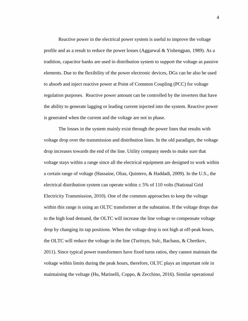
system provide great benefits, however, they also bring some challenges. Figure 1 depicts

a distribution system feeder where power may flow in two directions due to the delivery

of the exceeding power of the DG to the grid. Since this bidirectional power flow is

through the power lines, current generated losses exist as heat dissipation and as a result

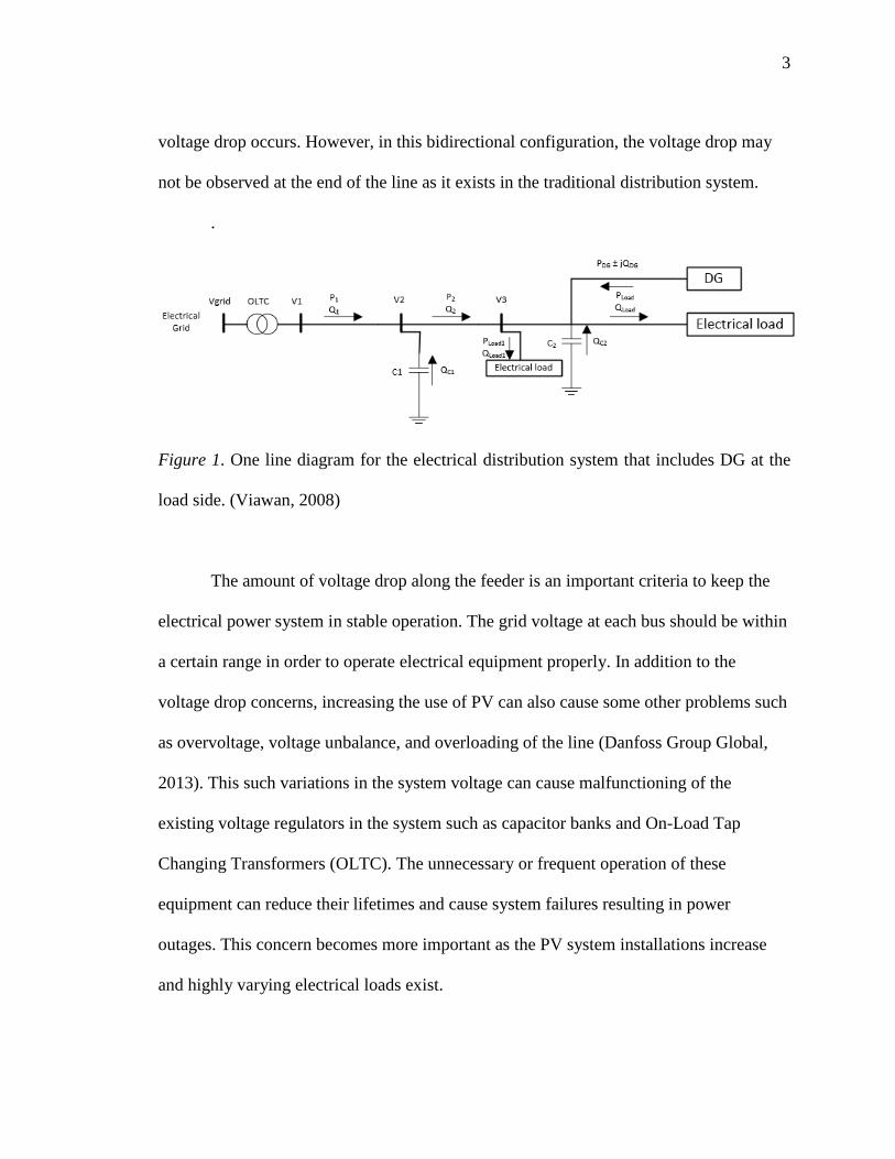
3

voltage drop occurs. However, in this bidirectional configuration, the voltage drop may

not be observed at the end of the line as it exists in the traditional distribution system.

.

Figure 1. One line diagram for the electrical distribution system that includes DG at the

load side. (Viawan, 2008)

The amount of voltage drop along the feeder is an important criteria to keep the

electrical power system in stable operation. The grid voltage at each bus should be within

a certain range in order to operate electrical equipment properly. In addition to the

voltage drop concerns, increasing the use of PV can also cause some other problems such

as overvoltage, voltage unbalance, and overloading of the line (Danfoss Group Global,

2013). This such variations in the system voltage can cause malfunctioning of the

existing voltage regulators in the system such as capacitor banks and On-Load Tap

Changing Transformers (OLTC). The unnecessary or frequent operation of these

equipment can reduce their lifetimes and cause system failures resulting in power

outages. This concern becomes more important as the PV system installations increase

and highly varying electrical loads exist.

4

Reactive power in the electrical power system is useful to improve the voltage

profile and as a result to reduce the power losses (Aggarwal & Yishengpan, 1989). As a

tradition, capacitor banks are used in distribution system to support the voltage as passive

elements. Due to the flexibility of the power electronic devices, DGs can be also be used

to absorb and inject reactive power at Point of Common Coupling (PCC) for voltage

regulation purposes. Reactive power amount can be controlled by the inverters that have

the ability to generate lagging or leading current injected into the system. Reactive power

is generated when the current and the voltage are not in phase.

The losses in the system mainly exist through the power lines that results with

voltage drop over the transmission and distribution lines. In the old paradigm, the voltage

drop increases towards the end of the line. Utility company needs to make sure that

voltage stays within a range since all the electrical equipment are designed to work within

a certain range of voltage (Hassaine, Olias, Quintero, & Haddadi, 2009). In the U.S., the

electrical distribution system can operate within ± 5% of 110 volts (National Grid

Electricity Transmission, 2010). One of the common approaches to keep the voltage

within this range is using an OLTC transformer at the substation. If the voltage drops due

to the high load demand, the OLTC will increase the line voltage to compensate voltage

drop by changing its tap positions. When the voltage drop is not high at off-peak hours,

the OLTC will reduce the voltage in the line (Turitsyn, Sulc, Bachaus, & Chertkov,

2011). Since typical power transformers have fixed turns ratios, they cannot maintain the

voltage within limits during the peak hours, therefore, OLTC plays an important role in

maintaining the voltage (Hu, Marinelli, Coppo, & Zecchino, 2016). Similar operational

5

principle exits for capacitor banks. They are connected to the PCC during the peak

hours. They have the capability to generate reactive power to regulate the voltage at the

PCC.

Statement of Problem

It is important to keep the electrical power grid voltage at each bus within a

certain range in order to operate equipment properly. Increasing the use of PV can cause

some problems such as overvoltage, voltage unbalance, and overloading. The variations

in the system voltage can cause malfunctioning of the existing voltage regulators in the

system such as capacitor banks and OLTC transformers. The unnecessary or frequent

operation of these equipment can reduce their lifetimes and cause system failures results

with power outages. This concern becomes more important as the PV system installations

increase and highly varying electrical loads exist. The coordination between the PV

systems and other DGs can improve the performance of the electrical grid and reduce the

losses. In 2015, the U.S Energy Information Administration (EIA) mentioned in the

annual report that transmission and distribution systems losses are around 5% of the total

energy generated which costs the US around $9 billion annually (US Energy Information

Administration, 2017).

Purpose of the Study

The purpose of this study is to provide a coordinated control method for the

power systems voltage profile when high numbers of PV farms are connected to the

electrical distribution system. It also provides an analysis of the unbalanced electrical

distribution system voltage profile. In addition, it proposes solution to reduce the number

6

of tap changes in the OLTC in the unbalanced system that includes high penetrated PV

systems. The proposed method provides coordination between different types of DGs to

improve the voltage control equipment performance by reducing electrical losses. This

study provides many optimal solutions to reduce the losses in the electrical distribution

systems using Genetic Algorithm.

Need for the Study

Changing the vertically integrated grid paradigm to the bidirectional paradigm

will increase the reliability and the robustness of the distribution system since there will

be many distributed energy sources supplying the increased electrical demand in

electrical grid from different locations. Improving PV’s performance will help to

maintain the voltage profile of the system and as a result reduce the number of tap

changes for the OLTC at the substation. Reduce in the OLTC operation result with

increase in the life time. Voltage regulation at each bus in the distribution system is

highly important in order to increase the use of PV. All the electrical devices are designed

to operate with a certain amount of voltage with a certain tolerance. Operating the

electrical devices outside the acceptable range can reduce the life cycle of the equipment

and in other cases can damage it. There are many ways to regulate the voltage at the

PCCs such as capacitor banks, and load shedding. This study uses the reactive power

control generated from the PVs to regulate the voltage at the PCCs. It also uses Genetic

Algorithm (GA) optimization to find the optimal point of operation for each device.

Assumptions of the Study

The following assumptions are made during this study:

7

The surround temperature is not involved in any calculations. The overall efficiency of

100% the PV is used in the simulation. The output power of a PV has a linear relationship

with the temperature.

Research Question

This study will discuss the following research questions:

1. How can coordinated control improve the voltage profile of an unbalanced distribution

system?

2. Would PV reduce the OLTC operation?

3. How can OLTC and PV system control unbalanced distribution system voltage?

4. How can GA optimize the distribution system to reduce the electrical losses?

Limitations of the Study

The following limitations are to be applied to this study:

1. The algorithm was implemented only in IEEE 13 bus system.

2. The price of the electricity generated by the PV is not considered.

3. The process time of the simulation is based on the Personal Computer (PC) used

capability.

4. The inverters used in reactive power control characteristics are not considered.

CHAPTER 2

LITERATURE REVIEW

8

The studies in the history of PV systems yield growing implementations in power

system in order to reduce the COR2R emissions in the atmosphere. However, increasing PV

installation can cause some technical challenges in the future which become more

concern for the utility companies and system operators. This literature review presents

the latest studies in reactive power control using PV and GA optimization in the

distribution system. The literature review is classified in five categories as PV systems,

inverters, reactive power control, OLTC, and GA.

UPV

Photovoltaic is the scientific expression of converting the energy of the light to

electrical energy. The word consists of two parts. Photo which is a Greek word means

light. Voltaic is named for the famous scientist Alessandro Volta (Overstraeton &

Mertens, 1986). The phenomena builds a voltage difference between two points which

allow a direct current (DC) pass through the medium. The source of energy that is

converted to electrical energy through the solar cells is the energy in the sun light. The

output voltage varies according to the amount of light on the panel surface. The amount

of power from the light could be measured using the solar irradiance. Solar irradiance is

radiant power incident per unit area on the surface with a unit of W/mP

2P. There is a direct

proportional relation between the output power from the PV system and the solar

irradiance. In most cases, the peak power for the PV inverter is measured with 1KW/mP

2

Pat 25 degree centigrade.

Current- voltage (I-V) and power-voltage (P-V) curves describe the performance

of the PV. They can be drawn as a variable with temperature or irradiance. Figure 2

9

provides the I-V curve with different irradiances. For each curve, the intersection with the

Y axis is the short circuit current which is the maximum current that the PV can supply in

case of short circuit at that specific irradiance level. For each curve, the intersection with

the X axis is the open circuit voltage which is the PV terminal voltage when there is no

load connected. The more irradiance the PV has the more current that can generate.

Figure 2. I-V curve with different irradiances Retrieved from (Jayakrishan, Kothari, Nedumgatt, Umashankar, & Vijayakumar, 2011)

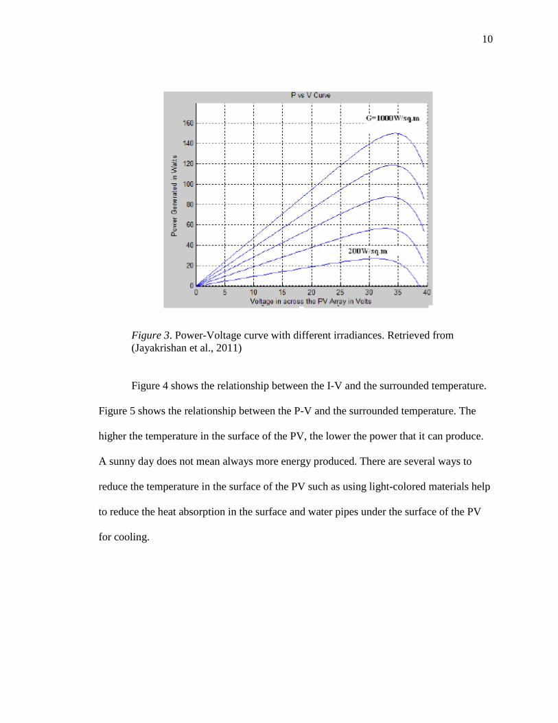
P-V characteristic varies according to the irradiance as well. Figure 3 shows that

the more irradiance the PV has the more power it can generate. After a certain point the

power will drop even the voltage is increasing. The ideal operation point should be just

before the power drops.

10

Figure 3. Power-Voltage curve with different irradiances. Retrieved from (Jayakrishan et al., 2011)

Figure 4 shows the relationship between the I-V and the surrounded temperature.

Figure 5 shows the relationship between the P-V and the surrounded temperature. The

higher the temperature in the surface of the PV, the lower the power that it can produce.

A sunny day does not mean always more energy produced. There are several ways to

reduce the temperature in the surface of the PV such as using light-colored materials help

to reduce the heat absorption in the surface and water pipes under the surface of the PV

for cooling.

11

Figure 4. I-V curve with different temperature. Retrieved from (Jayakrishan et al., 2011)

Figure 5. P-V curve with different temperature. Retrieved from (Jayasekara, Wolfs, & Masoum, 2014)

12

UInverters

R RInverter plays an important role in connecting the PV with the electrical grid. The

inverter is responsible for converting the DC produced by the PV to Alternating Current

(AC) to be connected to the electrical grid. There are different ways of connecting the PV

to the inverters. It varies according to the applications, and number of PV. Different types

of connection will be discussed as follows:

U1. Centralized inverters.

This technique was common in the past, but it is not common nowadays. A large

number of PVs are connected in series with a single phase inverter to establish a string to

generate high voltage, and then many strings are connected in parallel to generate high

power. There are some disadvantages of this approach such as a huge amount of high

voltage DC cables are need to connect the PVs together, power loss because of the

centralized Maximum Power Point Tracking (MPPT), harmonics, and power quality

issues (Kjaer, Pederson, & Blaabjerg, 2005).

U2. String Inverters and AC Modules.

This connection is the most common technique today. The approach is the

modified version of the centralized inverter’s approach where strings are not connected in

parallel. Approximately 16 PVs are connected in a string and one inverter is used. The

open circuit voltage can reach 720 V and the normal operation voltage can reach between

450 and 510 V. This approach increases the efficiency as the power loss is reduced (Kjaer

et al., 2005).

13

U3. Multi string inverters.

In this technique, each string is connected to a DC-DC converter to control the

input voltage for the inverter. It is more efficient as each converter can control a group of

PVs according to the needs. It provides flexibility to connect more PVs in the future

unless the power does not exceed the maximum power of the inverter. It is easier to

maintain as the operator can disconnect the converter and some PVs without effecting the

operation of the others. The inverter is responsible to generate the appropriate voltage to

be connected to the electrical grid. A feedback signal from the electrical grid is sent to the

inverter to adjust the output voltage from the inverter. Many researchers are working in

this approach because it has higher efficiency than others. Improving the respond time

and the performance of the inverter will improve the whole system (Kjaer et al., 2005).

U4. AC-Module Technology.

This technique is a standalone approach where each PV unit has its own inverter.

These individual inverters are also called as micro-inverters which provides easy

connection. Most of the PV units in this technique is not designed for high power

generation. It is still expensive because of the technology used, but it is expected to be

cheaper in the future as technology improves (Kjaer et al., 2005).

UReactive Power Control

Inverters are the key components that connect the PV with the AC grid through

converting DC output to AC. By controlling the operation of the inverter, PV systems can

inject or absorb reactive power. Voltage control in distribution system through reactive

power generated by PV systems is addressed in many studies in the literature. In 2010,

14

Albuquerque, Moraes, Guimaraes, Sanhueza, and Vaz. presented an algorithm to control

the reactive power generation in PV. The algorithm used in inverter control is based on

two errors and one parameter. The first error between the PV DC output voltage, and

reference dc voltage. This error is used to control the active power in the PV inverter. The

second error between the PV current output and reference current is used to control the

reactive power. If the voltage grid is greater than 220V (nominal voltage), the system will

absorb reactive power. If it is less than 220V, the system will inject reactive power. PI

controllers are used to minimize the error as a result to control active and reactive power

(Albuquerque et al., 2010).

In 2011, Hamzaoui, Bouchafaa, and Hadjammar used fuzzy logic to control

Maximum Power Point Tracker (MPPT). A PI fuzzy logic regulator is used for the Pulse

Width Modulation (PWM). Power reference is calculated from a DC-bus voltage

controller to be used as a reference for MPPT. Error between the references and the

estimated feedback power are input to the hysteresis comparators. The authors created

look up tables for the reactive power error is at a certain level so that the PWM will have

an assured phase angle difference between the voltage and the current for reactive power

control (Hamzaoui et al., 2011).

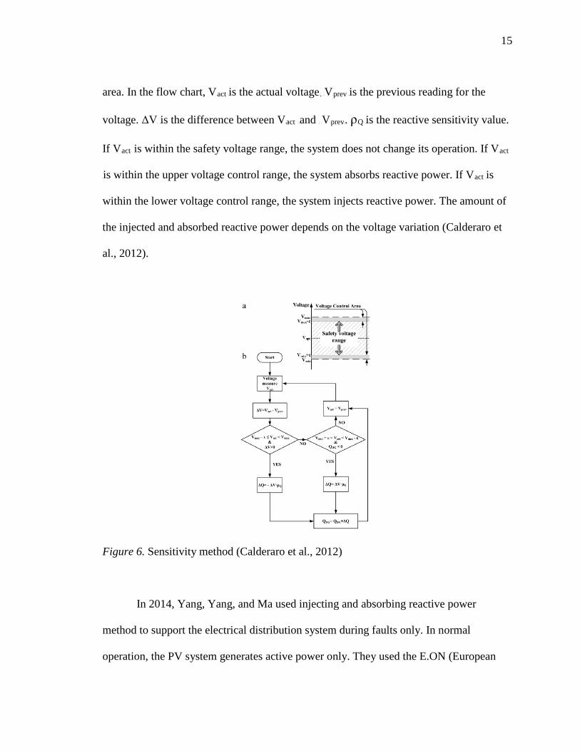
Calderaro, Conio, Galdi, and Piccolo presented a method in 2012 called as

sensitivity method that controls the wind turbine output voltage through reactive power

control. In implementing the sensitivity, the maximum and minimum voltages have to be

identified so that the system runs within the safety voltage range. The system should be

running within the safety voltage range. ε is safety factor that defines the voltage control

15

area. In the flow chart, VRact Ris the actual voltageR. RVRprev Ris the previous reading for the

voltage. ΔVR Ris the difference between VRact Rand R RVRprevR. ρRQ Ris the reactive sensitivity value.

If VRactR is within the safety voltage range, the system does not change its operation. If VRact

Ris within the upper voltage control range, the system absorbs reactive power. If VRact Ris

within the lower voltage control range, the system injects reactive power. The amount of

the injected and absorbed reactive power depends on the voltage variation (Calderaro et

al., 2012).

Figure 6. Sensitivity method (Calderaro et al., 2012)

In 2014, Yang, Yang, and Ma used injecting and absorbing reactive power

method to support the electrical distribution system during faults only. In normal

operation, the PV system generates active power only. They used the E.ON (European

16

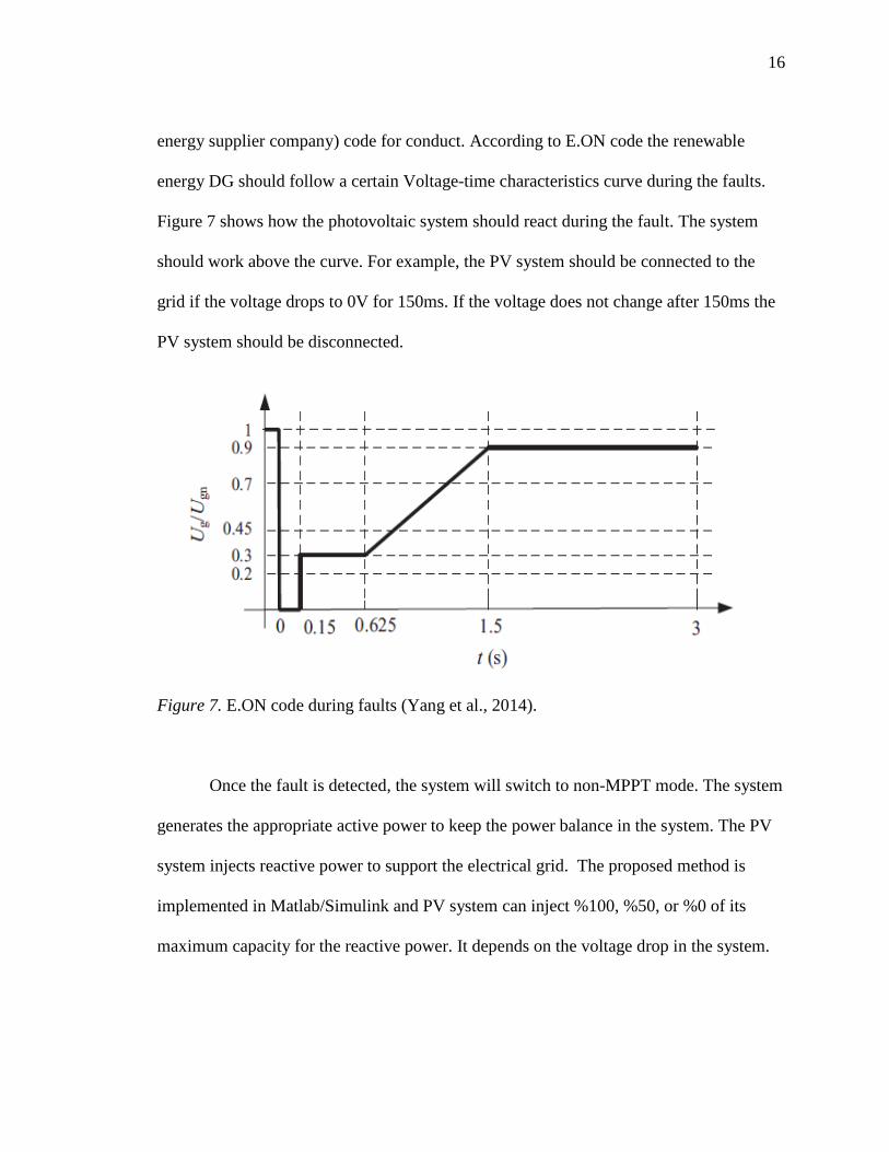
energy supplier company) code for conduct. According to E.ON code the renewable

energy DG should follow a certain Voltage-time characteristics curve during the faults.

Figure 7 shows how the photovoltaic system should react during the fault. The system

should work above the curve. For example, the PV system should be connected to the

grid if the voltage drops to 0V for 150ms. If the voltage does not change after 150ms the

PV system should be disconnected.

Figure 7. E.ON code during faults (Yang et al., 2014).

Once the fault is detected, the system will switch to non-MPPT mode. The system

generates the appropriate active power to keep the power balance in the system. The PV

system injects reactive power to support the electrical grid. The proposed method is

implemented in Matlab/Simulink and PV system can inject %100, %50, or %0 of its

maximum capacity for the reactive power. It depends on the voltage drop in the system.

17

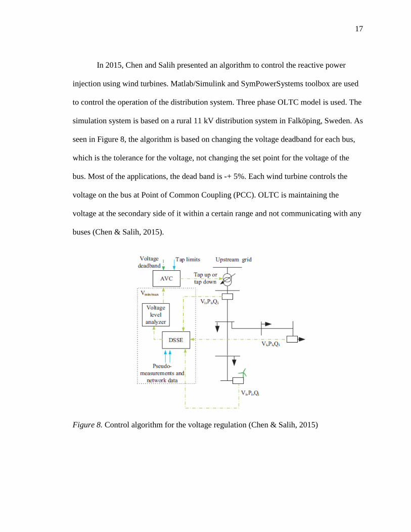
In 2015, Chen and Salih presented an algorithm to control the reactive power

injection using wind turbines. Matlab/Simulink and SymPowerSystems toolbox are used

to control the operation of the distribution system. Three phase OLTC model is used. The

simulation system is based on a rural 11 kV distribution system in Falköping, Sweden. As

seen in Figure 8, the algorithm is based on changing the voltage deadband for each bus,

which is the tolerance for the voltage, not changing the set point for the voltage of the

bus. Most of the applications, the dead band is -+ 5%. Each wind turbine controls the

voltage on the bus at Point of Common Coupling (PCC). OLTC is maintaining the

voltage at the secondary side of it within a certain range and not communicating with any

buses (Chen & Salih, 2015).

Figure 8. Control algorithm for the voltage regulation (Chen & Salih, 2015)

18

In 2015, Nazir, Kanada, Syafii, and Coveria used Newton-Raphson method to

control reactive power. They calculated the values of ma (Index modulation) which is the

amplitude of the inverter output voltage and alpha which is the grid phase angle. The

turns ratio between the VRinvR and VRsupplyR is given as a. The inverter injects or absorbs

reactive power based on ma and alpha. The amount of reactive power can be determined

by the value of ma and the injection or absorption can be determined by the value of

alpha. (Nazir et al., 2015).

𝐺𝐺(𝑚𝑚𝑚𝑚, 𝛿𝛿) = 𝐺𝐺𝐺𝐺 = (𝑉𝑉𝑉𝑉𝑉𝑉/�2)𝑎𝑎𝑎𝑎𝑉𝑉𝑋𝑋

sin 𝛿𝛿 - P =0 (1)

𝐻𝐻(𝑚𝑚𝑚𝑚, 𝛿𝛿) = 𝐻𝐻𝐺𝐺 = (𝑉𝑉𝑉𝑉𝑉𝑉/�2)𝑎𝑎𝑎𝑎𝑉𝑉𝑋𝑋

cos 𝛿𝛿 − 𝑉𝑉2/𝑋𝑋 =0 (2)

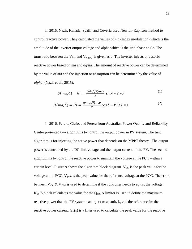
In 2016, Perera, Ciufo, and Perera from Australian Power Quality and Reliability

Centre presented two algorithms to control the output power in PV system. The first

algorithm is for injecting the active power that depends on the MPPT theory. The output

power is controlled by the DC-link voltage and the output current of the PV. The second

algorithm is to control the reactive power to maintain the voltage at the PCC within a

certain level. Figure 9 shows the algorithm block diagram. VRgm Ris the peak value for the

voltage at the PCC. VRgm0 Ris the peak value for the reference voltage at the PCC. The error

between VRgmR & VRgm0 Ris used to determine if the controller needs to adjust the voltage.

KRpqR/S block calculates the value for the QRref. RA limiter is used to define the maximum

reactive power that the PV system can inject or absorb. IRqrefR is the reference for the

reactive power current. Gcc(s) is a filter used to calculate the peak value for the reactive

19

current output IRgq. RGvgq(s) is the model for the Q algorithm controller. It is a close loop

control system where VRgm Ris measured all the time and used for as a feedback (Perera et

al., 2016).

Figure 9. Q controller algorithm (Perera et al., 2016)

The authors provided two case studies to control the reactive power. The first case

is to inject a fixed minimum lagging power factor. The lagging power factor can be

maintained at 0.95. The active power changes according to the operation, and the

controller injects or absorbs reactive power to maintain the lagging power factor always

at 0.95. In this case, the PV does not generate the maximum output power all the time.

The minimum lagging power factor is used to minimize the losses and over loading. In

this case, the PV may be disconnected if the active power reached a certain level. The

second case is to generate the maximum apparent power. The active power changes

according to the demand, and then the PV inverter injects or absorbs reactive power until

it reaches the maximum apparent power for the PV system. In this case, the PV should

always be connected to the PCC to regulate the voltage.

In 2016, Rafi, Hossain, and Lu presented five different modes of operation for

voltage regulation with off-line-tap changer where the tap changer has to be disconnected

20

from the system to change the tap position. The system is a residential area in Australia

that includes three and single phase system, PV system, Battery Energy Storage (BES),

and Static Synchronous Compensators (STATCOM). Each PV system produces 4.5 KW

and 5KVA and supplies ten customers. If the PV generation is less than the electrical

demand, it operates in normal operation mode (mode A). The system is monitoring the

faults, and voltage level. The STATCOM and the BES are still available in mode A.

Mode B is when the PV generation is higher than the electrical demand and the PCC

voltage is greater than 1.06 per unit (pu) (over voltage case). The STATCOM works with

full capacity to regulate the voltage. If the voltage is still above 1.06 pu the BES starts to

charge the batteries. If the voltage still needs to be regulated, the system uses active

power curtailment approach. The last option is to shut down some particular PV sections

(Rafi et al., 2016).

Mode C is when the PV injects and absorbs reactive power. This mode was

implemented recently in some areas in Australia. It is cheaper than using BES

installations. The system is limited to either 0.95 or 0.90 lagging power factor operation.

The control system is based on the theory of de-rating power control. It means that there

is a limit for the active power which allows some capacity for the reactive power. Mode

D is to combine mode B and C together. The STATCOM regulates the voltage, then the

BES. The last option is to inject or absorb reactive power using PV. In addition to mode

D, DG power sharing is presented in Mode E. In power sharing, all the DGs share the

loads based on the power rating for each DG. The system was designed using

PSCAD/EMTDC (Rafi et al., 2016).

21

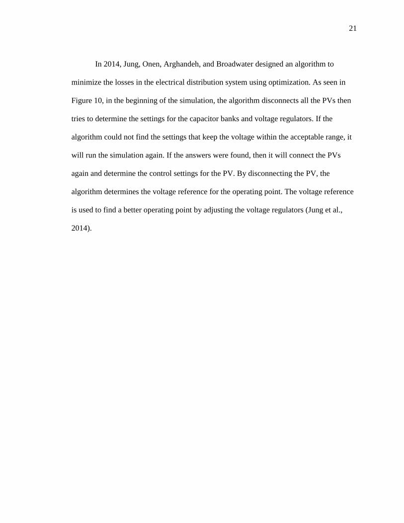
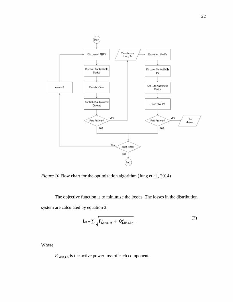
In 2014, Jung, Onen, Arghandeh, and Broadwater designed an algorithm to

minimize the losses in the electrical distribution system using optimization. As seen in

Figure 10, in the beginning of the simulation, the algorithm disconnects all the PVs then

tries to determine the settings for the capacitor banks and voltage regulators. If the

algorithm could not find the settings that keep the voltage within the acceptable range, it

will run the simulation again. If the answers were found, then it will connect the PVs

again and determine the control settings for the PV. By disconnecting the PV, the

algorithm determines the voltage reference for the operating point. The voltage reference

is used to find a better operating point by adjusting the voltage regulators (Jung et al.,

2014).

22

Figure 10.Flow chart for the optimization algorithm (Jung et al., 2014).

The objective function is to minimize the losses. The losses in the distribution

system are calculated by equation 3.

Ln = ∑�PLoss,i,n2 + QLoss,i,n

2 R

(3)

Where

𝑃𝑃Loss,i,n Ris the active power loss of each component.

23

𝑄𝑄Loss,i,nis the reactive power loss of each component.

There are three constraints in this study. The tap position, voltage in each bus, and

the power factor should be within a certain range. The software used to optimize the

system was not mentioned.

In 2016, Haque and Wolfs provided more options to regulate the voltage during

high PV penetrations. They presented the reconductoring as a possible method to regulate

the voltage. Reconductoring depends on increasing the cross-sectional area of the feeder

cables. Figure 11 shows reducing the line reactance X and line resistance R can reduce

the voltage drop across the feeders. Increasing cross-sectional area of the cables reduces

the values for X and R. Reconductoring is a very efficient method to regulate the voltage,

but it is very expensive. This method could be valuable during the design for a new

system, but most of the time it is not practical for an existent system.

Figure 11. Single line diagram for a distribution system (Haque & Wolfs, 2016).

On-Load Voltage Regulator based on Electronic Power Transformer (OLVR-

EPT) was presented in the Haque and Wolfs paper. It is a new technology to replace the

OLTC which reduces the physical weight, harmonics, and voltage drop in the

24

transformer, provides faster and continuous voltage regulation, however, they are very

expensive. There is no need to use mechanical tap changers in OLVR-EPT. Increased

reliability and availability will encourage many companies to use it. There are other

methods to regulate the voltage such as using fixed and switched capacitor banks, which

is a common method has been used for years. Switching capacitors are used in discrete a

step that means it is on or off state. The reactive power demand changes continuously and

the whole capacitance value might not be needed (Haque & Wolfs, 2016).

The Haque and Wolfs paper provided coordination method between the power

station utilities equipment and the PV. The method is based on using batteries. The

voltage rises during the off-peak hours. The coordination controller sends a signal to

charge the batteries to absorb the reverse power. The voltage drops during the peak hours.

The coordination controller sends a signal to discharge the batteries to maintain the

voltage within a certain level. This paper also presented the reactive power control in the

PV system. It presented an algorithm to maintain the voltage at the PCC within an

acceptable range. The algorithm is based on generating the maximum active power from

the PV and using the rest of PV’s capacity to generate the reactive power. The system

was simulated in a small scale using a Texas Instruments floating point TMS320F28335

Digital Signal Processor. The reactive power is limited as the active power is maximum

in all cases of study (Haque & Wolfs, 2016).

UGenetic Algorithm

Genetic Algorithm is one of the optimization techniques. It is based on the theory

of genetics and natural selection. GA was developed by John Holland in 1975. In 1989,

25

David Goldberg used GA to solve the problem with the gas-pipeline transmission control.

It was the first time to use GA to solve a control problem (Haupt & Haupt, 2004). GA is

not the best technique to solve all the optimization problems. There are some advantages

of using GA such as:

- Can optimize continuous or discrete variables.

- Can solve a large number of parameters.

- Can run with parallel computers.

- Can optimize complex systems.

Objective function is the function that the GA is trying to minimize or maximize.

GA generates some random potential solutions to solve the objective function. The

solutions are called the chromosomes. Each chromosome contains number of genes to

define the chromosome and explain its characteristics. The chromosomes that do not

optimize the objective function will be eliminated. The chromosomes that optimize the

objective function will generate another generation to optimize the objective function by

reproduction (Ramos, 2014).

In 2011, Riffonneau, Bacha, Barruel, and Ploix used the optimization process to

reduce the operation costs by managing the power flow and using PV systems and energy

storage batteries as a power system application of optimization. In this study, the forecast

data for irradiance, temperature, and loads consumption profiles were used to manage the

power flow. The objective function of this study is:

26

CF(∆t) = [Pgrid(∆t) × FIT(∆t) × ∆t] + [Pgrid(∆t) × EgP(∆t) ×

BrC(∆t)]

(4)

where

CF is cash flow.

PRGRID RpowerR Rgrid.

FiT feed-in tariff.

EgP electricity grid price.

BrC the battery’s replacement cost.

There are five constraints for the objective function:

PRGRID R(t) = PRPV R(t) + PRBAT R(t) + PRLOADS R(t) (5)

SOCP

minP ≤ SOC (t) ≤ SOCP

max (6)

PRBATRP

minP ≤ PRBATR (t) ≤ PRBATRP

max (7)

SOH (t) ≥ SOHP

min (8)

PRGRIDR (t) ≤ PRGRIDRP

max (9)

where

PRPV Rthe output power from PV

PRBATR the output power from battery

PRLOADS Rtotal power for the loads.

SOC state of charge, which shows how much charge the battery has. 0% is empty.

100% is full.

SOH state of health. It is the condition of the battery compared to the ideal

condition. The ideal condition is a 100% at the time of manufacture.

27

The Riffonneau et al. study was implemented using RT-Lab HILBox 4U that can

handle real-world interfacing using fast input/output boards for hardware-in-the-loop

applications. The simulation was implemented using Matlab/Simulink where some RT-

Lab blocks were used. This study did not control reactive power in the PV system. It was

listed as a future work (Riffonneau et al., 2011).

In 2012, Kolenc, Papic, and Blazic designed an algorithm to minimize the OLTC

operation and the losses in the distribution system based on an operating point which is

the ratio between the reactive power and the active power generated by a DG. The

operating point has to be ±3 %. The algorithm searches for the optimal operating point

for each feeder to make sure that the voltage does not exceed 1.05pu or below 0.95 pu. A

load forecast is running with the simulation to determine if it is economically effective to

change the tap position. The algorithm has been simulated by DIgSILENT Power Factory

simulation program and MATPOWER. 20 kV medium-voltage Slovenian distribution

system was used to test the algorithm. OLTC controls ±12% of the rated voltage with

1.33% for each tap position (Kolenc et al., 2012).

In 2014, Ramos used GA to optimize the operation of distributed generation. The

objective function is the power losses in the system. PV systems were used to inject or

absorb reactive power to minimize the power losses. The objective function of Ramos

study is:

PRloss R= ∑ 𝐺𝐺𝐺𝐺𝑛𝑛𝑏𝑏𝑘𝑘=1 [VRkRP

2P + VRmRP

2P – 2VRkRVRm cos(𝜃𝜃𝐺𝐺 − 𝜃𝜃𝐺𝐺)] (10)

where

nb the number of branches.

28

PRloss Rthe power loss.

Gk is the conductance of the line.

R R VRk R& VRm Rare the voltage at bus k and m.

θRk R&R RθRm Rare the phase angles at bus k and m.

The Ramos study had only one constraint for the reactive power injection and

absorption. The reactive power is limited between 0.95 inductive and 0.95 capacitive.

OLTC was not part of the objective function. MATLAB is used to optimize a modified

IEEE system (Ramos, 2014).

In 2014, Yang et al. presented an algorithm to minimize the losses in the

distribution system. The simulation was implemented using Visual Studio C++ and

multi-phase distribution network model UBLF. CPLEX solver was used to solve the

optimization problem. The optimization was designed as a mixed integer quadratic

optimization problem. The algorithm was tested and verified for nine different

distribution systems. The distribution systems were divided into two categories. The first

one includes control the reactive power using capacitors. The second one includes

capacitors and reactive power generated from different DGs. OLTC was not part of any

distribution systems. The objective function is to minimize the losses by reducing the

active and reactive current as seen in equation 11.

Min F = ∑ ��Iid�2 + �Iiq�2�nb

𝑖𝑖=1 × 𝑟𝑟i (11)

Where

Iid, Iiq is the active and reactive current in branch i.

𝑟𝑟i Ris the resistance of branch i.

29

The constraints in the Yang et al. study include a limitation for the current, the

voltage, the maximum reactive power, the minimum reactive power, the line-to-neutral

voltage, and line-to-line voltage.

In 2016, Harnett used Frank – Wolfe algorithm to optimize the power flow in the

electrical distribution system. The algorithm focuses on running the system safely when

there is a problem in the electrical distribution system such as overvoltage, and faults.

Harnett used MATPOWER for the simulation. The voltage regulation was done by

existing voltage regulators such as capacitors and injecting reactive power using wind

turbine and generators. Harnett also focused on using optimization to find the weakest

point in the electrical distribution system. The weakest point is the point where if it has a

failure, the failure can cause a black out and it will be difficult to recover. Harnett

mentioned that knowing the weakest point in the grid will be very useful for the smart

grid. Finding the weakest point can help to design the electrical grid so that it can handle

some issues at the weakest point. Harnett did not regulate the voltage using PV and

OLTC (Harnett, 2016).

UOLTC

Transmitting electricity causes voltage drop over the transmission and distribution

lines. The voltage at the beginning of the line is higher than the voltage at the end of the

line when there is an inductive load that is the case for power systems. The longer the

transmission line is, the more voltage drop in the end. All the electrical equipment is

designed to work within a certain level of voltage (Hassaine et al., 2009). In the US, the

electrical distribution system can operate within ± 5% of 110 volts (National Grid

30

Electricity Transmission, 2010). That means the equipment at the end of the distribution

lines could face the risk of having voltage less than 110 volts. The common approach to

solve this problem is using an OLTC transformer at the substation. It allows the

transformer to adjust the voltage to keep the voltage within limits. If the voltage drops

due to the load demand is high, the OLTC will increase the voltage in the line to

compensate that voltage drop by changing its tap positions. At night when the voltage

drop is not high, the OLTC will reduce the voltage in the line (Turitsyn et al., 2011). The

peak times are in the morning when the residents are getting ready for work and in the

afternoon when they come back from work. For the commercial areas, the peak time is

around noon. If there is no work shift at night the electrical demand is low.

OLTC has been one of the main components in the electrical network for the past

90 years. It not only maintains the secondary voltage within a certain range, but also used

for phase shifting. The main types of OLTC are high-speed-resistor type and reactor type.

Resistor type is used in large transformers and reactor type is used in small transformers.

The changer is installed inside the transformer. OLTC changes the turns ratio for the

transformer by changing the tap position. The voltage could be increased or decreased

based on the tap position. The tap change could be installed in the primary or the

secondary side of the transformer. As show in Figure 12, the reactor or the resistance is

used as a bridge to transfer the loads from one tap to another without any shutdown or

interruption. During changing the tap position, the current is divided between two taps to

reduce the probability of having sparks during the transition (Dohnal, 2013).

31

Figure 12. Reactor and resistor principle. (Dohnal, 2013)

USummary

In the literature review there are some researches that are focusing on reducing

the power losses in the distribution system. In 2014, Ramos presented an algorithm to

minimize the losses, but the OLTC was not involved in this simulation. In 2016, Perera et

al. from Australian Power Quality and Reliability Centre presented an algorithm to

reduce the power losses. The algorithm was limited to 0.9 lagging power factor and was

not designed to operate with different lagging power factor. Some of the researches are

designed based on forecasting data such as the study presented by Marko, Igor, and

Boštjan. Any big change between the forecasting and actual data will cause inaccurate

decisions. The study was designed to reduce the power losses as well.

32

Some other studies were focusing in maintaining the voltage within the acceptable

range without looking at the power losses in the distribution system. Albuquerque et al.,

2010 presented an algorithm to regulate the voltage using reactive power generated from

the PV system. They used PI controller to control the reactive power. Hamzaoui et al.

presented a fuzzy logic control system to regulate the voltage. The system was built to

regulate the voltage by changing the MPPT. There are some researches that present the

voltage regulation only under some circumstances such as the research presented by

Yang et al. in 2014. The PV regulates the voltage only during the fault condition in the

electrical system. If the fault is still exist after 10ms the PV system will be disconnected.

A three phase controlled system for the PV was presented by and Chen and Salih in 2015.

In their system, the decision to inject or absorb reactive power is based on one phase and

the change happens simultaneously for the three phases. In 2016, Rafi et al. used storage

batteries and STATCOM to regulate the voltage. When there is a small electrical

demand, the system charges the batteries. The charged batteries will be used during the

peak hours or when the PV cannot generate enough power due to low irradiance.

The literature review also presented some research using optimization in the

electrical distribution system. In 2014, Ramos used GA to reduce the losses in the

distribution system. The algorithm given by Ramos was three phase controlled system.

The above mentioned studies considered the voltage control of a distribution

system in many different aspects. Some considers the existing regulators and others

focused on the PV inverter control. However, there is limited studies exists that considers

33

coordination between the PV inverters and existing regulators and more specifically not

for unbalanced distribution system.

This Dissertation proposes a coordinated control method between the existing

regulators and PV inverters for the power system voltage profile when high numbers of

PV farms are connected to the electrical distribution system. This study also provides an

analysis and voltage regulation of the unbalanced electrical distribution system voltage

profile. Mix integer nonlinear optimization problem is solved using genetic algorithm to

define the PI controller parameters while not considering the details of power electronic

devices. Matlab and co-simulation of Simulink are used to implement the algorithm on

IEEE 13 bus unbalanced distribution system.

UScope of the Research

Voltage regulation in unbalanced system has been investigated for many years.

The researchers try to regulate the voltage generated from each source of energy

connected to the electrical distribution. Implementing the bidirectional paradigm

encourages the researchers to investigate how to use different sources of energy in

voltage regulation. In the decade, using PV system in voltage regulation has been

investigated. It has been tested and verified, but there are some gaps in this field such as

no study to simulate a single phase controlled inverter for the PV system. In addition,

there is no study to simulate single phase controlled OLTC. All the simulations have been

done to control all the three phases simultaneously. There is no study that optimizes

OLTC and PV system to reduce the electrical losses using GA.

34

This research provides a single phase controlled inverter PV model and a single

phase controlled OLTC model. It provides an optimization system for OLTC and PV

system using GA with the objective function of minimizing the line losses. All the

simulations are done using Matlab/Simulink, and Simulation optimization.

35

CHAPTER 3

METHODOLOGY

There are many parameters that can be adjusted in the electrical distribution

system such as OLTC tap position, generator parameters, and capacitor bank switch

states to increase the stability and reduce the cost of operation through loss minimization.

Power systems uses optimization processes to find the optimum values for these

parameters to be a stable system. Optimization is a well-known method used in power

systems such as in unit commitment (Patriksson, Andreasson, & Evgrafov, 2017). In

addition, optimization is used commonly in control systems to find the best control

parameters for better response.

The proposed voltage control scheme is considered for an unbalanced distribution

system that includes OLTC, capacitor bank and PV systems at the user side. The method

utilizes PV system inverters to provide reactive power to the distribution system. In

addition, it considers the existing voltage control devices (OLTC and Capacitor)

operation and aims to keep their operations in minimum to increase their life time. The

voltage control of unbalanced network is achieved with single phase voltage control

where the individual line impedances are considered. By minimizing the overall system

losses, coordinated control of the OLTC and PV reactive power is achieved using Genetic

Algorithm for loss minimization. The PI controllers used to control reactive power of the

PVs are tuned through the optimization process. The proposed method is implemented

using Matlab Optimization Toolbox and co-simulation of Simulink model of IEEE 13 bus

36

system for more accurate and detail control and results. The following subsections

present the details of problem formulation and its solution as optimization.

UUnbalanced Distribution System Voltage

The unbalanced distribution network and its voltage profile is analyzed using

IEEE 13 bus unbalanced distribution system test case. The network is modeled using

Matlab Simulink and the existing OLTC model. The PV reactive power control affect is

investigated by adding PV systems at different locations over the network where the

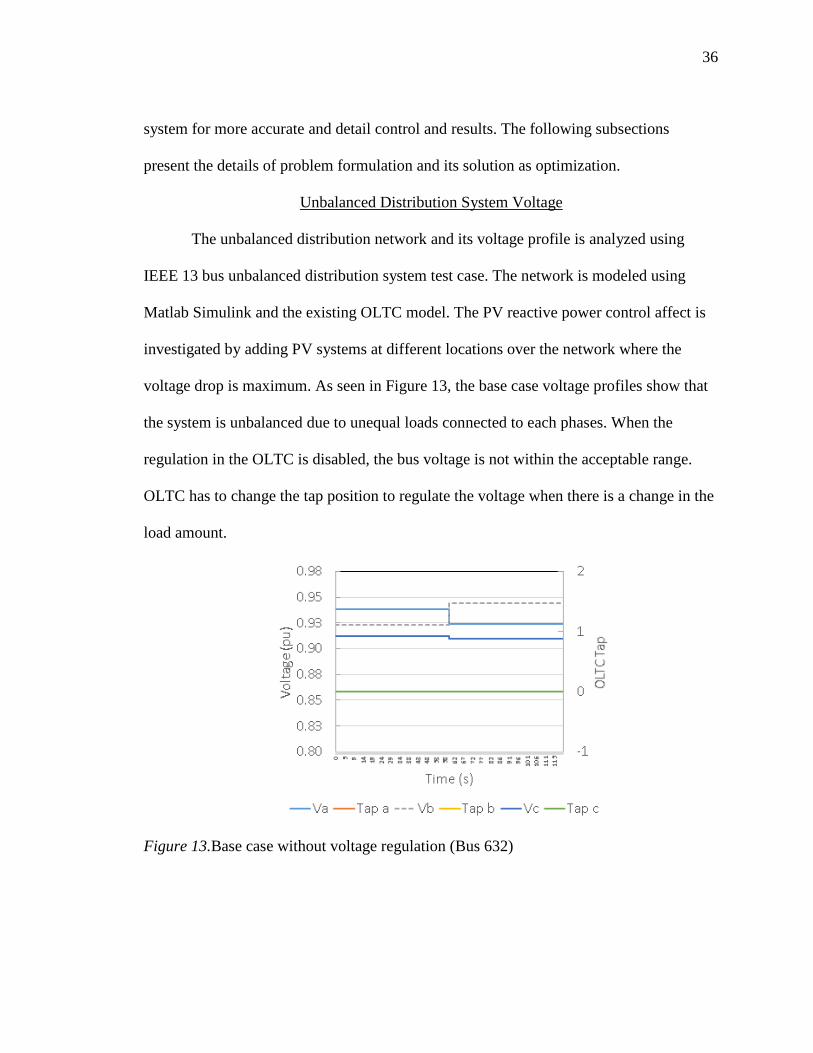
voltage drop is maximum. As seen in Figure 13, the base case voltage profiles show that

the system is unbalanced due to unequal loads connected to each phases. When the

regulation in the OLTC is disabled, the bus voltage is not within the acceptable range.

OLTC has to change the tap position to regulate the voltage when there is a change in the

load amount.

Figure 13.Base case without voltage regulation (Bus 632)

37

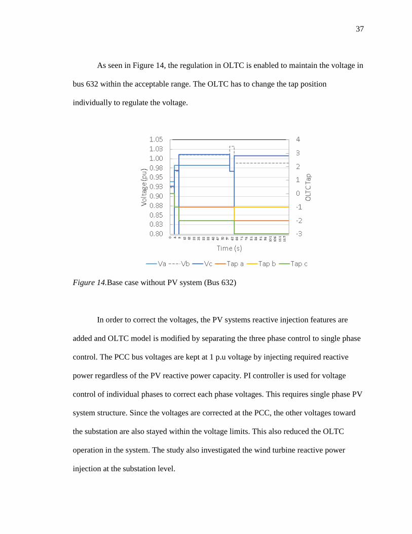
As seen in Figure 14, the regulation in OLTC is enabled to maintain the voltage in

bus 632 within the acceptable range. The OLTC has to change the tap position

individually to regulate the voltage.

Figure 14.Base case without PV system (Bus 632)

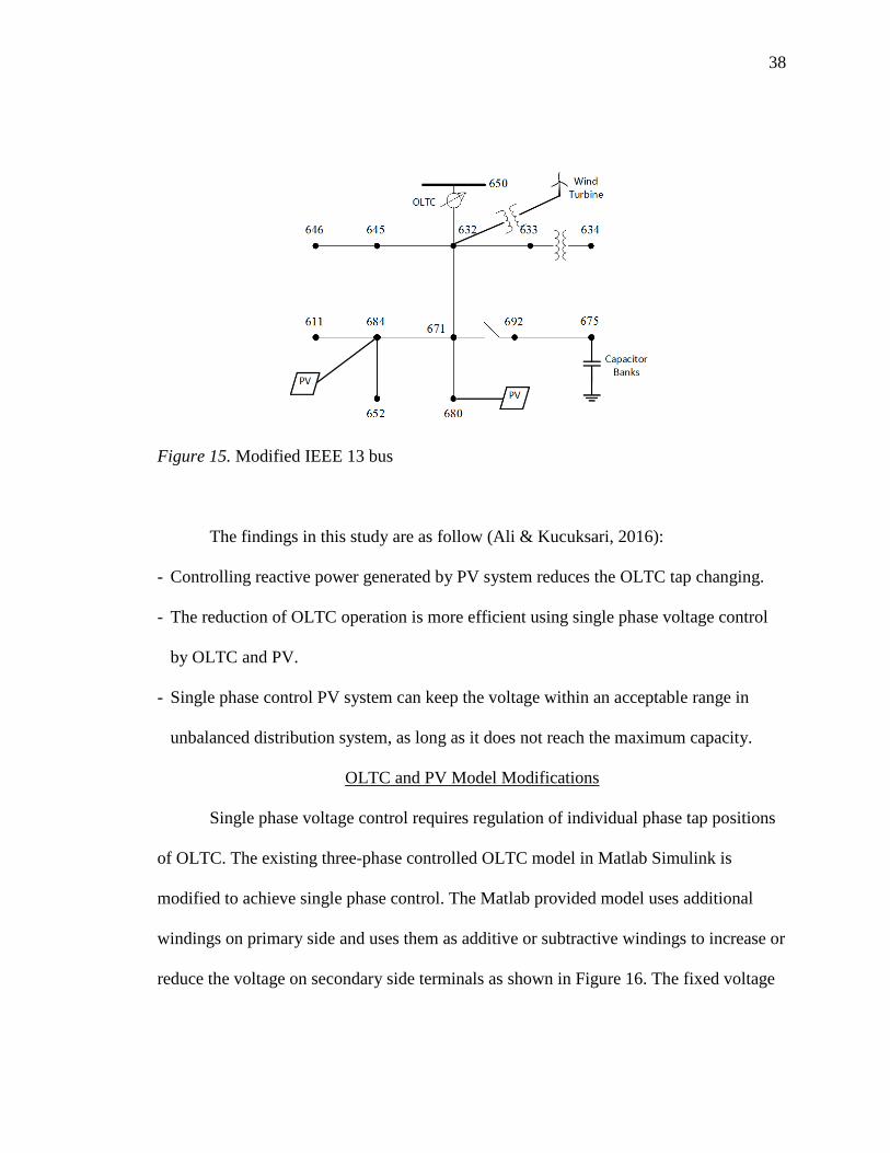
In order to correct the voltages, the PV systems reactive injection features are

added and OLTC model is modified by separating the three phase control to single phase

control. The PCC bus voltages are kept at 1 p.u voltage by injecting required reactive

power regardless of the PV reactive power capacity. PI controller is used for voltage

control of individual phases to correct each phase voltages. This requires single phase PV

system structure. Since the voltages are corrected at the PCC, the other voltages toward

the substation are also stayed within the voltage limits. This also reduced the OLTC

operation in the system. The study also investigated the wind turbine reactive power

injection at the substation level.

38

Figure 15. Modified IEEE 13 bus

The findings in this study are as follow (Ali & Kucuksari, 2016):

- Controlling reactive power generated by PV system reduces the OLTC tap changing.

- The reduction of OLTC operation is more efficient using single phase voltage control

by OLTC and PV.

- Single phase control PV system can keep the voltage within an acceptable range in

unbalanced distribution system, as long as it does not reach the maximum capacity.

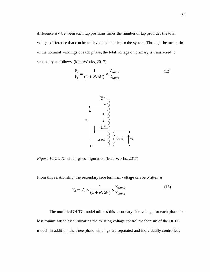
UOLTC and PV Model Modifications

Single phase voltage control requires regulation of individual phase tap positions

of OLTC. The existing three-phase controlled OLTC model in Matlab Simulink is

modified to achieve single phase control. The Matlab provided model uses additional

windings on primary side and uses them as additive or subtractive windings to increase or

reduce the voltage on secondary side terminals as shown in Figure 16. The fixed voltage

39

difference ∆V between each tap positions times the number of tap provides the total

voltage difference that can be achieved and applied to the system. Through the turn ratio

of the nominal windings of each phase, the total voltage on primary is transferred to

secondary as follows (MathWorks, 2017):

𝑉𝑉2𝑉𝑉1

=1

(1 + 𝑁𝑁.∆𝑉𝑉)×𝑉𝑉𝑛𝑛𝑛𝑛𝑎𝑎2𝑉𝑉𝑛𝑛𝑛𝑛𝑎𝑎1

(12)

Figure 16.OLTC windings configuration (MathWorks, 2017)

From this relationship, the secondary side terminal voltage can be written as

𝑉𝑉2 = 𝑉𝑉1 ×1

(1 + 𝑁𝑁.∆𝑉𝑉)×𝑉𝑉𝑛𝑛𝑛𝑛𝑎𝑎2𝑉𝑉𝑛𝑛𝑛𝑛𝑎𝑎1

(13)

The modified OLTC model utilizes this secondary side voltage for each phase for

loss minimization by eliminating the existing voltage control mechanism of the OLTC

model. In addition, the three phase windings are separated and individually controlled.

40

The PV model used in this study is the available model in Matlab Simulink. The model is

also modified to inject reactive power. In addition, the three-phase designed model is

converted to single-phase design and PI controllers for each phase are added to control

the reactive power. The actual inverter model is not considered since the focus is not

given to its control.

UCoordinated Voltage Control through Loss Minimization

The voltage drop in power systems is mainly due the heat dissipated power IP

2PxR

on the transmission and distribution lines. This is only the active power portion of the

losses. There are system losses due to the reactive power as well. The losses are high in

distribution system since the X/R ratio of the conductors is high and the current amount

on these conductors is higher. In order to improve the voltage profile in the system, the

minimization of the overall system losses is crucial. The total system losses are the sum

of individual line losses which can be express as Ptotal loss = ∑ 𝑃𝑃𝑖𝑖𝑖𝑖𝑖𝑖𝑖𝑖=1 R where j is the total

number of line sections between the busses in the system. The individual line active

power losses can be express as 𝑃𝑃𝑖𝑖 = 𝐼𝐼𝑖𝑖2 × 𝑅𝑅𝑖𝑖 where I is the line current, i is the bus

number, and R is the line resistance. Pi can also be expressed in terms of the bus voltage

and line resistance as 𝑃𝑃𝑖𝑖 = �𝑉𝑉𝑖𝑖+1−𝑉𝑉𝑖𝑖|𝑍𝑍𝑖𝑖|�2

× 𝑅𝑅𝑖𝑖. Same relationship can be used to calculate the

line losses for the line between i and i+1 where the OLTC secondary side is connected to

bus i+1 as follows:

𝑃𝑃𝑖𝑖 = �𝑉𝑉𝑖𝑖+1 − 𝑉𝑉𝑖𝑖

|𝑍𝑍𝑖𝑖|�2

× 𝑅𝑅𝑖𝑖 (14)

41

𝑃𝑃𝑖𝑖 =(𝑉𝑉1 × 1

(1 + 𝑁𝑁.∆𝑉𝑉) × 𝑉𝑉𝑛𝑛𝑛𝑛𝑎𝑎2𝑉𝑉𝑛𝑛𝑛𝑛𝑎𝑎1

− 𝑉𝑉𝑖𝑖)2

|𝑍𝑍𝐿𝐿𝐺𝐺𝐿𝐿𝐿𝐿|2 × 𝑅𝑅𝑖𝑖

(15)

where VR1R is the OLTC primary side voltage and 𝑅𝑅𝑖𝑖 is the resistance of the line between

busses 𝐺𝐺 and 𝐺𝐺 + 1.

The reactive power effects the line losses since the total current over the line has

active and reactive power components. The 𝑃𝑃𝑖𝑖 = 𝐼𝐼𝑖𝑖2 × 𝑅𝑅𝑖𝑖 line losses can be written in

terms of active and reactive power flowing through the line as:

𝑃𝑃𝑖𝑖 = 𝐼𝐼𝑖𝑖2 × 𝑅𝑅𝑖𝑖 = �𝑆𝑆𝑖𝑖𝑉𝑉𝑖𝑖�2

× 𝑅𝑅𝑖𝑖 = ��𝑃𝑃𝑖𝑖 + 𝑄𝑄𝑖𝑖

𝑉𝑉𝑖𝑖�2

=𝑃𝑃𝑖𝑖2 + 𝑄𝑄𝑖𝑖2

𝑉𝑉𝑖𝑖2× 𝑅𝑅𝑖𝑖

(16)

This relation shows that if reactive power is injected by a PV or capacitor as

negative Q, the line losses can be reduced since the total circuit current drops.

In order to minimize the system losses, Genetic Algorithm (GA) is selected as the

optimization algorithm since the power systems is a nonlinear system with several

constrains. The total loss that needs to be minimized becomes the fitness function for GA.

The decision variables for minimization are the reactive power amount of the PV, the

turn on and off state of capacitor if exists, and OLTC tap position all of which affect the

line losses as explained earlier. The system constrains during the minimization are the

voltage limits, reactive power capacity of the PV inverter, OLTC tap numbers, and

capacitor on and off states. The capacitor on and off states are binary, therefore, the

42

overall fitness function becomes a mix-integer nonlinear problem and can be formed for j

number of bus system as:

𝑃𝑃𝑇𝑇𝑛𝑛𝑇𝑇𝑎𝑎𝑇𝑇 𝑇𝑇𝑛𝑛𝑙𝑙𝑙𝑙 = 𝑚𝑚𝐺𝐺𝐿𝐿 �(𝑉𝑉1× 1

(1+𝑁𝑁.∆𝑉𝑉)×𝑉𝑉𝑛𝑛𝑛𝑛𝑛𝑛2𝑉𝑉𝑛𝑛𝑛𝑛𝑛𝑛1

−𝑉𝑉2)2×𝑅𝑅𝑖𝑖

|𝑍𝑍𝐿𝐿𝑖𝑖𝑛𝑛𝐿𝐿|2 + ∑𝑃𝑃𝑖𝑖2+�𝑄𝑄𝐿𝐿𝑖𝑖±𝑥𝑥𝑖𝑖𝑖𝑖𝑄𝑄𝐶𝐶𝐶𝐶𝐶𝐶𝑖𝑖+𝑄𝑄𝑃𝑃𝑉𝑉𝑖𝑖�

2

𝑉𝑉𝑖𝑖2 × 𝑅𝑅𝑖𝑖

𝑖𝑖𝑖𝑖=2 � R(17)

The system constrains are:

−𝑁𝑁𝑇𝑇𝑎𝑎𝑇𝑇 ≤ 𝑁𝑁 ≤ 𝑁𝑁𝑇𝑇𝑎𝑎𝑇𝑇

𝑥𝑥𝑖𝑖𝑉𝑉 = 0 or 1

−𝑄𝑄𝑃𝑃𝑉𝑉𝑖𝑖𝑛𝑛𝐶𝐶𝑖𝑖 ≤ 𝑄𝑄𝑃𝑃𝑉𝑉𝑖𝑖 ≤ 𝑄𝑄𝑃𝑃𝑉𝑉𝑖𝑖𝑛𝑛𝐶𝐶𝑖𝑖

0.95 𝑝𝑝.𝑢𝑢 ≤ 𝑉𝑉𝑖𝑖 ≤ 1.05 𝑝𝑝. 𝑢𝑢

where

VR1R the grid voltage.

N the tap position in the OLTC.

NRTapR is the number of taps in the OLTC

ΔV is the voltage difference between two tap positions in the OLTC.

VRnom1R is the nominal voltage in the primary side of the OLTC.

VRnom2 Ris the nominal voltage in the secondary side of the OLTC.

R is the transmission line resistance of line.

P is the load power at bus.

QRLR is the load reactive power.

QRCapR is the capacitor reactive power.

QRPVR is the reactive power generated by the PV.

43

The function that needs to be minimized has basically two parts; (1) the line right

after the OLTC, and (2) the other lines. Although both parts are same lines in terms of

construction, the difference is on the formulation of the losses. As it is clearly seen that

the first part is a variable of the OLTC tap positions and the others are variable of

reactive power of the PV and capacitor if exists.

In addition to direct control of PV reactive power QPVi in the objective function,

PI controller is used for dynamic voltage control of individual phases to correct each

phase voltages. The error for the PI controller is determined by comparing the actual

voltage with 1 pu reference voltage. The error is used as input for PI controller. The

output from the PI controller is the reactive power injected or absorbed by PV that is used

in the formulation. During the optimization, GA determines the values for KRP Rand KRI , Ras

a result, the PI controller decides on reactive power amount to regulate the voltage either

through injecting or absorbing reactive power. The PI controller generates the required Q

as

𝑄𝑄(𝑠𝑠) = (𝐾𝐾𝑇𝑇 + 𝐾𝐾𝑖𝑖1𝑙𝑙) 𝐸𝐸𝑟𝑟𝑟𝑟𝐸𝐸𝑟𝑟(𝑠𝑠) (18)

KRPR is the proportional constant.

KRIR is the integral constant.

The proposed algorithm has been implemented in Matlab and Simulink. Matlab

optimization toolbox, parallel pool toolbox, and Simulink Simpower systems toolbox are

used for optimization through simulation. The flow chart given in Figure 17 shows the

process flow. Optimization starts with initial values of zeros. GA generates the first

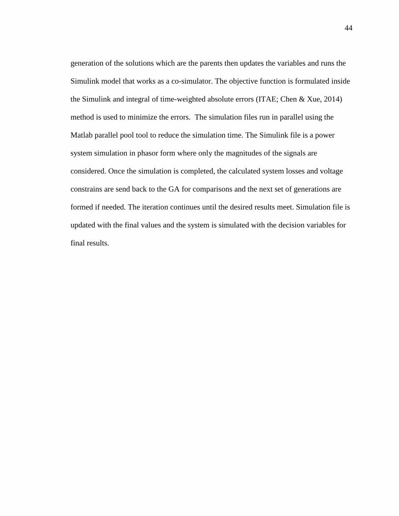
44

generation of the solutions which are the parents then updates the variables and runs the

Simulink model that works as a co-simulator. The objective function is formulated inside

the Simulink and integral of time-weighted absolute errors (ITAE; Chen & Xue, 2014)

method is used to minimize the errors. The simulation files run in parallel using the

Matlab parallel pool tool to reduce the simulation time. The Simulink file is a power

system simulation in phasor form where only the magnitudes of the signals are

considered. Once the simulation is completed, the calculated system losses and voltage

constrains are send back to the GA for comparisons and the next set of generations are

formed if needed. The iteration continues until the desired results meet. Simulation file is

updated with the final values and the system is simulated with the decision variables for

final results.

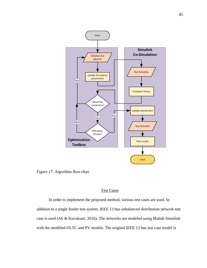
45

Figure 17. Algorithm flow chart

UTest Cases

In order to implement the proposed method, various test cases are used. In

addition to a single feeder test system, IEEE 13 bus unbalanced distribution network test

case is used (Ali & Kucuksari, 2016). The networks are modeled using Matlab Simulink

with the modified OLTC and PV models. The original IEEE 13 bus test case model is

Start

Initialize the parents

Update Simulation parameters

Run Simulink

Evaluate Fitness

Meet the constrains?

Minimum Fitness?

Yes

No

NoRun Simulink

Yes

Update parameters

End

Plot results

Simulink Co-Simulation

Optimization Toolbox

46

first developed as base case and simulated to verify that the system is unbalanced and

voltage drops are observed. PV systems are added as three phase active power sources

only. It is verified that the active power injection of the PV systems are not helping the

voltage profile. In order to bring the voltage drops to desired range, the PV systems

reactive power injection features are added and OLTC model is modified by separating

the three phase control for positive sequence and single phase controls separately. The PI

controllers’ reference input are set to 1 since the PCC bus voltages are desired to be 1 p.u

The following three case studies are performed by the test system:

Case 1: Single feeder distribution system contains OLTC, PV, capacitor, and

electrical load. The algorithm is controlling the reactive power generated by the PV,

OLTC tap position, and the capacitor bank operation.

Case 2: PV system and capacitor bank connected to bus 675 of IEEE 13-bus

system. The algorithm controls the system based on the positive sequence of unbalanced

system voltage.

Case 3: PV system and capacitor bank connected to bus 675 of IEEE 13-bus

system. The algorithm controls the system voltage as three single phase system.

Case 4: Dynamic load is added to bus 680 of IEEE 13 bus system used in case 3

and variable irradiance is implemented to the PV system.

.

47

CHAPTER 4

RESULTS AND DISCUSSIONS

This chapter discusses the cases of study and their results. It also provides some

analyses to the data and explains how the algorithm works in each case.

Case 1

A simple simulation study has been conducted using Matlab/Simulink to verify

the proposed method and its implementation. Figure 18 shows the three phase, three bus

balanced distribution system that includes OLTC, three phase electrical load, three phase

capacitor bank, and PV system. Three phase load contains 500 kW active power and 200

kVAR reactive power. The numbers are selected such that a voltage drop exists at the end

of the line. The objective function is minimizing the total line losses and the decision

variables are the OLTC tap position, turning on and off state of the capacitor bank, and

injecting or absorbing reactive power amount of the PV. GA optimizes the tap position,

capacitor on and off state, and reactive power amount that needs to be injected or absorb

by PV. The PV reactive power is controlled by PID controller. Equations 8 through 11

show the objective function in this case of study. The details of the Line 1 power loss

calculation in terms of OLTC tap position is provided in equation 20. OLTC is controlled

by controlling the N in the objective (fitness) function.

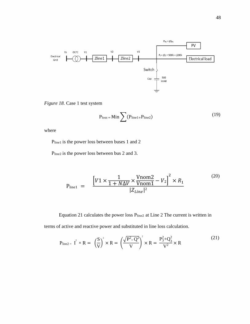
48

Figure 18. Case 1 test system

Ploss = Min�(Pline1+Pline2) (19)

where

Pline1 Ris the power loss between buses 1 and 2

Pline2 Ris the power loss between bus 2 and 3.

Pline1 = �𝑉𝑉1 × 1

1 + 𝑁𝑁∆𝑉𝑉 × Vnom2Vnom1 − 𝑉𝑉2�

2× 𝑅𝑅1

|𝑍𝑍𝐿𝐿𝑖𝑖𝑛𝑛𝐿𝐿|2

(20)

Equation 21 calculates the power loss Pline2R at Line 2 The current is written in

terms of active and reactive power and substituted in line loss calculation.

Pline2 = I2

× R = �SV�

2

× R = ��P2

+ Q2

V�

2

× R = P3

2+Q32

V2 × R (21)

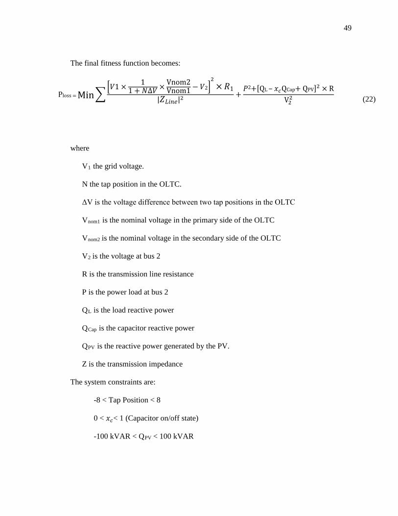
49

The final fitness function becomes:

Ploss = Min��𝑉𝑉1 × 1

1 + 𝑁𝑁∆𝑉𝑉 × Vnom2Vnom1 − 𝑉𝑉2�

2× 𝑅𝑅1

|𝑍𝑍𝐿𝐿𝐺𝐺𝐿𝐿𝐿𝐿|2 +𝑃𝑃2+[QL – 𝑥𝑥𝑉𝑉QCap+ QPV]2 × R

V22

(22)

where

VR1R the grid voltage.

N the tap position in the OLTC.

ΔV is the voltage difference between two tap positions in the OLTC

VRnom1R is the nominal voltage in the primary side of the OLTC

VRnom2 Ris the nominal voltage in the secondary side of the OLTC

VR2 Ris the voltage at bus 2

R is the transmission line resistance

P is the power load at bus 2

QRLR is the load reactive power

QRCapR is the capacitor reactive power

QRPVR is the reactive power generated by the PV.

Z is the transmission impedance

The system constraints are:

-8 < Tap Position < 8

0 < 𝑥𝑥𝑉𝑉< 1 (Capacitor on/off state)

-100 kVAR < QRPV R< 100 kVAR

50

0.95 pu < VR3 R< 1.05 pu

The decision variable of the system are, OLTC tap position, capacitor state, Kp,Ki, and

Kd values.

The circuit model is developed in Simulink as shown in Figure 19. The simulation

is part of the optimization process and controlled by a Matlab m-file. The optimization

uses parallel pool functionality of Matlab that utilizes 30 cores of the computer to reduce

the time for the iterations.

Figure 19. Circuit simulation in Simulink

51

One of the constraints is to keep the voltage at the PCC where the PV and

capacitor is connected within 0.95 p.u and 1.05 pu. When VR3R is within the range the rest

of the system voltage will be in acceptable range since Bus 3 is the end point in the line.

The optimization takes the VR3R as constrain during the optimization. Table 1 shows the

optimization results after 172 iterations.

Table 1

Optimization parameters (case 1)

OLTC

Tap position

Capacitor state

(on=1, off=0)

Kp Ki Kd

1 0 1,491 636 2,175

This optimization results for the decision variables are plugged into the simulation

and then run. Results show that the simulation can run successfully and the VR3R voltage

stays at 1 pu as shown in Figure 20. Bus 3 voltage reaches to 1 pu value in a very short

period of time which shows that the PID controller responses to the changes immediately.

Since the load power is constant through the simulation, once the VR3R reaches to 1 pu, it

stays there until the end of the simulation.

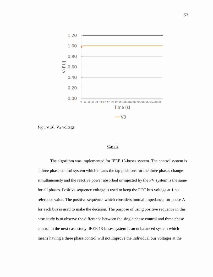
52

Figure 20. VR3R voltage

Case 2

The algorithm was implemented for IEEE 13-buses system. The control system is

a three phase control system which means the tap positions for the three phases change

simultaneously and the reactive power absorbed or injected by the PV system is the same

for all phases. Positive sequence voltage is used to keep the PCC bus voltage at 1 pu

reference value. The positive sequence, which considers mutual impedance, for phase A

for each bus is used to make the decision. The purpose of using positive sequence in this

case study is to observe the difference between the single phase control and three phase

control in the next case study. IEEE 13-buses system is an unbalanced system which

means having a three phase control will not improve the individual bus voltages at the

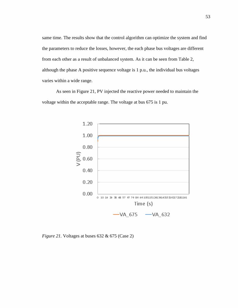
53

same time. The results show that the control algorithm can optimize the system and find

the parameters to reduce the losses, however, the each phase bus voltages are different

from each other as a result of unbalanced system. As it can be seen from Table 2,

although the phase A positive sequence voltage is 1 p.u., the individual bus voltages

varies within a wide range.

As seen in Figure 21, PV injected the reactive power needed to maintain the

voltage within the acceptable range. The voltage at bus 675 is 1 pu.

Figure 21. Voltages at buses 632 & 675 (Case 2)

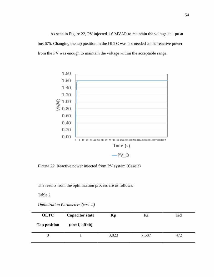
54

As seen in Figure 22, PV injected 1.6 MVAR to maintain the voltage at 1 pu at

bus 675. Changing the tap position in the OLTC was not needed as the reactive power

from the PV was enough to maintain the voltage within the acceptable range.

Figure 22. Reactive power injected from PV system (Case 2)

The results from the optimization process are as follows:

Table 2

Optimization Parameters (case 2)

OLTC

Tap position

Capacitor state

(on=1, off=0)

Kp Ki Kd

0 1 3,823 7,687 472

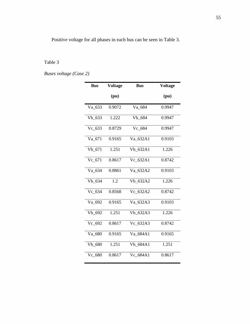
55

Positive voltage for all phases in each bus can be seen in Table 3.

Table 3

Buses voltage (Case 2)

Bus Voltage

(pu)

Bus Voltage

(pu)

Va_633 0.9072 Va_684 0.9947

Vb_633 1.222 Vb_684 0.9947

Vc_633 0.8729 Vc_684 0.9947

Va_671 0.9165 Va_632A1 0.9103

Vb_671 1.251 Vb_632A1 1.226

Vc_671 0.8617 Vc_632A1 0.8742

Va_634 0.8861 Va_632A2 0.9103

Vb_634 1.2 Vb_632A2 1.226

Vc_634 0.8568 Vc_632A2 0.8742

Va_692 0.9165 Va_632A3 0.9103

Vb_692 1.251 Vb_632A3 1.226

Vc_692 0.8617 Vc_632A3 0.8742

Va_680 0.9165 Va_684A1 0.9165

Vb_680 1.251 Vb_684A1 1.251

Vc_680 0.8617 Vc_684A1 0.8617

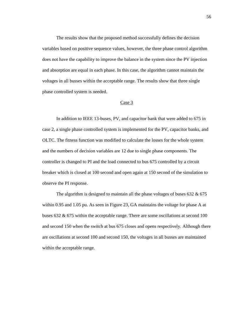
56

The results show that the proposed method successfully defines the decision

variables based on positive sequence values, however, the three phase control algorithm

does not have the capability to improve the balance in the system since the PV injection

and absorption are equal in each phase. In this case, the algorithm cannot maintain the

voltages in all busses within the acceptable range. The results show that three single

phase controlled system is needed.

Case 3

In addition to IEEE 13-buses, PV, and capacitor bank that were added to 675 in

case 2, a single phase controlled system is implemented for the PV, capacitor banks, and

OLTC. The fitness function was modified to calculate the losses for the whole system

and the numbers of decision variables are 12 due to single phase components. The

controller is changed to PI and the load connected to bus 675 controlled by a circuit

breaker which is closed at 100 second and open again at 150 second of the simulation to

observe the PI response.

The algorithm is designed to maintain all the phase voltages of buses 632 & 675

within 0.95 and 1.05 pu. As seen in Figure 23, GA maintains the voltage for phase A at

buses 632 & 675 within the acceptable range. There are some oscillations at second 100

and second 150 when the switch at bus 675 closes and opens respectively. Although there

are oscillations at second 100 and second 150, the voltages in all busses are maintained

within the acceptable range.

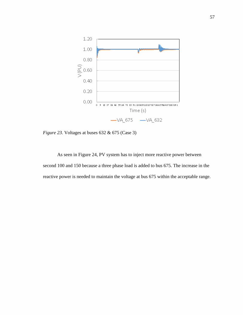
57


As seen in Figure 24, PV system has to inject more reactive power between

second 100 and 150 because a three phase load is added to bus 675. The increase in the

reactive power is needed to maintain the voltage at bus 675 within the acceptable range.

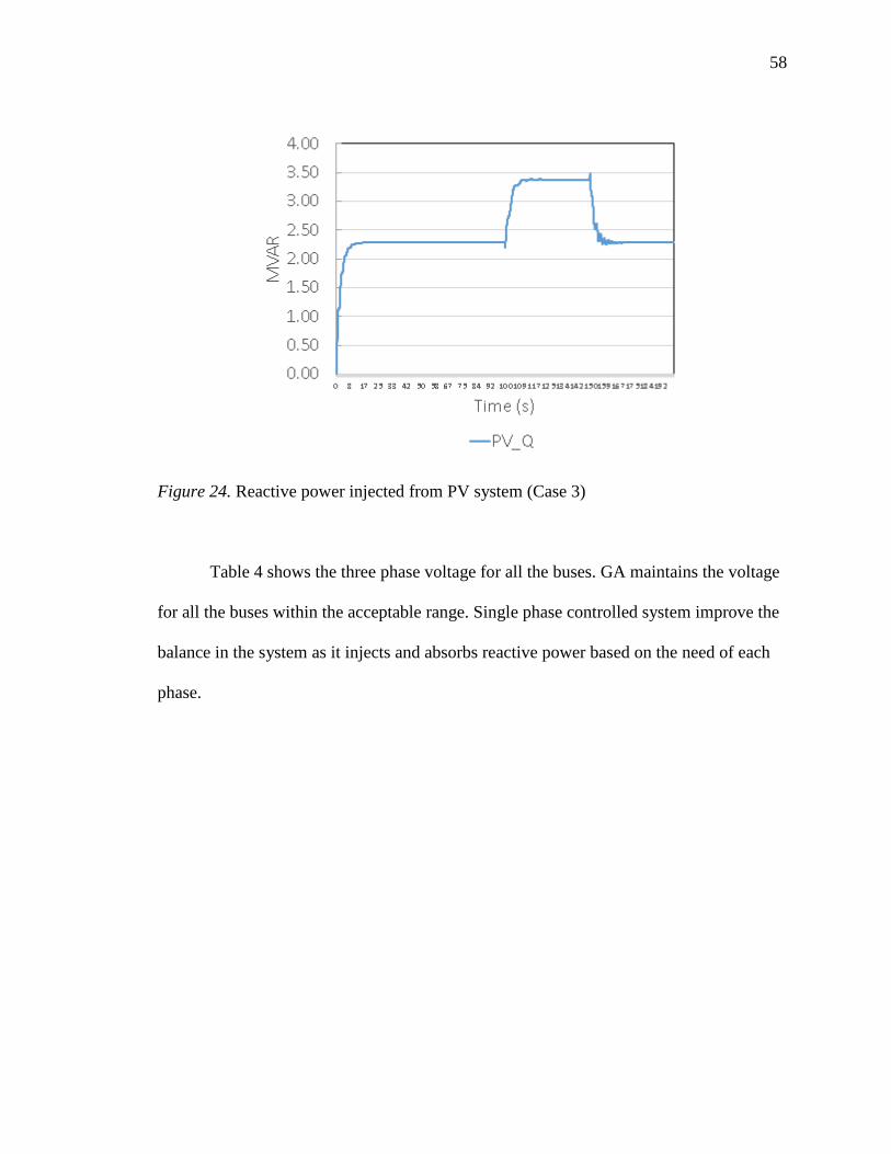
58


Table 4 shows the three phase voltage for all the buses. GA maintains the voltage

for all the buses within the acceptable range. Single phase controlled system improve the

balance in the system as it injects and absorbs reactive power based on the need of each

phase.

59

Table 4


Bus Voltage

(pu)

Bus Voltage

(pu)

Va_633 1.007 Va_684 0.9992

Vb_633 0.975 Vb_684 0.9952

Vc_633 0.9837 Vc_684 0.9917

Va_671 1.001 Va_632A1 1.011

Vb_671 0.9952 Vb_632A1 0.9768

Vc_671 0.9931 Vc_632A1 0.986

Va_634 0.9838 Va_632A2 1.011

Vb_634 0.957 Vb_632A2 0.9768

Vc_634 0.9655 Vc_632A2 0.986

Va_692 1.001 Va_632A3 1.011

Vb_692 0.9952 Vb_632A3 0.9768

Vc_692 0.9931 Vc_632A3 0.980

Va_680 1.001 Va_684A1 1.001

Vb_680 0.9952 Vb_684A1 0.9952

Vc_680 0.9931 Vc_684A1 0.9931

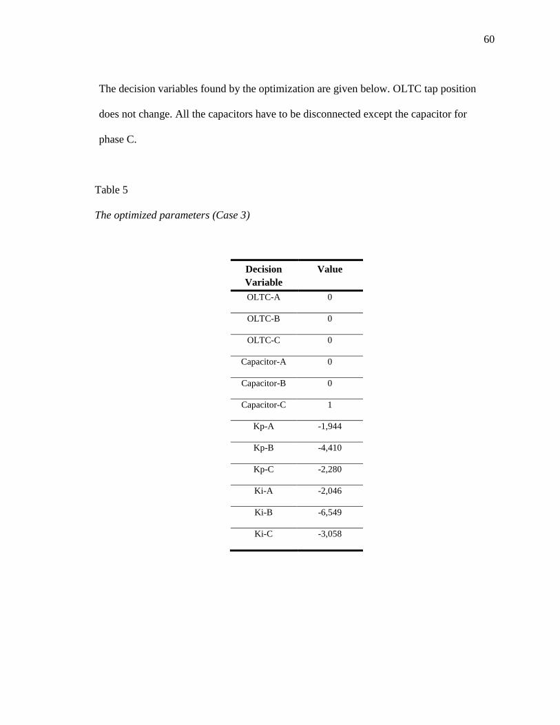
60

The decision variables found by the optimization are given below. OLTC tap position

does not change. All the capacitors have to be disconnected except the capacitor for

phase C.

Table 5

The optimized parameters (Case 3)

Decision Variable

Value

OLTC-A 0

OLTC-B 0

OLTC-C 0

Capacitor-A 0

Capacitor-B 0

Capacitor-C 1

Kp-A -1,944

Kp-B -4,410

Kp-C -2,280

Ki-A -2,046

Ki-B -6,549

Ki-C -3,058

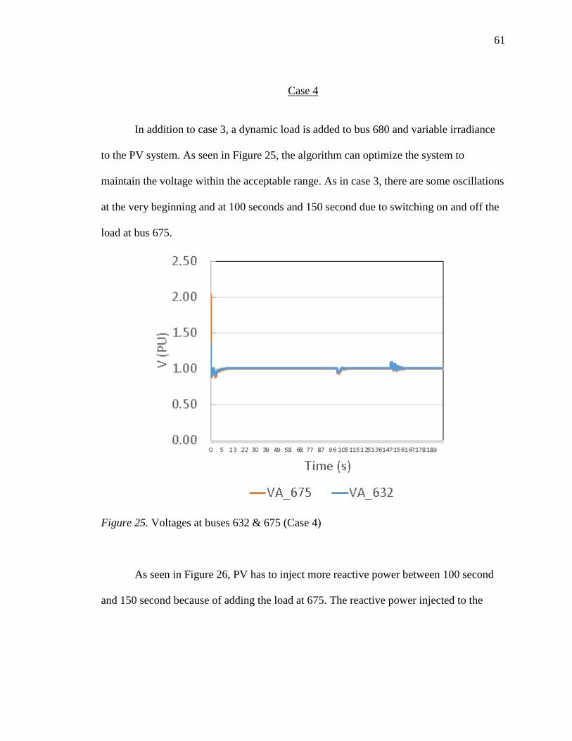
61

Case 4

In addition to case 3, a dynamic load is added to bus 680 and variable irradiance

to the PV system. As seen in Figure 25, the algorithm can optimize the system to

maintain the voltage within the acceptable range. As in case 3, there are some oscillations

at the very beginning and at 100 seconds and 150 second due to switching on and off the

load at bus 675.


As seen in Figure 26, PV has to inject more reactive power between 100 second

and 150 second because of adding the load at 675. The reactive power injected to the

62

system is following the same pattern as in case 3 with some changes due to the dynamic

load.


The voltage in each phase can be seen in Table 6.

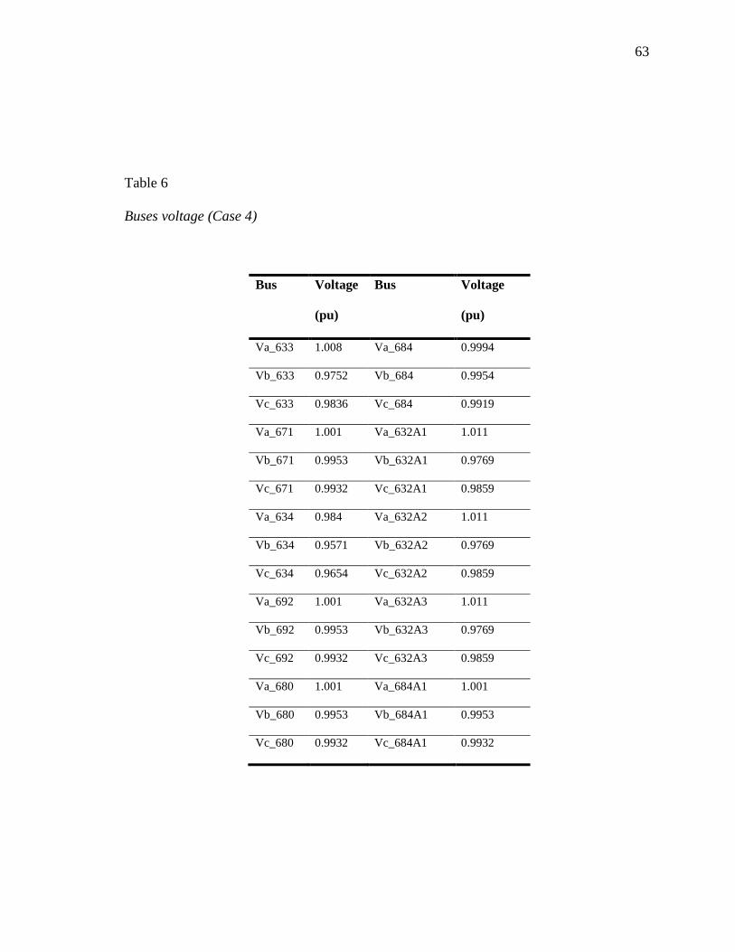
63

Table 6


Bus Voltage

(pu)

Bus Voltage

(pu)

Va_633 1.008 Va_684 0.9994

Vb_633 0.9752 Vb_684 0.9954

Vc_633 0.9836 Vc_684 0.9919

Va_671 1.001 Va_632A1 1.011

Vb_671 0.9953 Vb_632A1 0.9769

Vc_671 0.9932 Vc_632A1 0.9859

Va_634 0.984 Va_632A2 1.011

Vb_634 0.9571 Vb_632A2 0.9769

Vc_634 0.9654 Vc_632A2 0.9859

Va_692 1.001 Va_632A3 1.011

Vb_692 0.9953 Vb_632A3 0.9769

Vc_692 0.9932 Vc_632A3 0.9859

Va_680 1.001 Va_684A1 1.001

Vb_680 0.9953 Vb_684A1 0.9953

Vc_680 0.9932 Vc_684A1 0.9932

64

USummary

The proposed algorithm was tested and verified in case 1 in a small scale

distribution system. In case 2, the same algorithm was implemented in a bigger scale

system. The system was designed based on the positive sequence for each phase which is

not the best method to control the voltage in un-balanced distribution system. In case 3,

the system was designed as a three single phase controlled system. Case 3 showed the

ability to improve the balance in the distribution system by using three single phase

controlled system. The number of tap position changes for the OLTC is reduced

compared to the base case in Figure 13. Case 4 showed how the algorithm can handle a

dynamic load.

The results show the ability of GA to optimize electrical distribution system. It

also shows that the algorithm can optimize OLTC, and PV system with the ability to meet

the constraints in each case.

65

CHAPTER 5

CONCLUSION AND FUTURE RECOMMENDATIONS

PV system has been growing rapidly in the last decade. There are a lot of sectors

using PV system including commercial and residential applications. Chapter 1 introduced

the importance of the PV systems and how they grow rapidly. It also provided some

background about PV installation and the challenges facing it. Chapter 2 introduced

literature review about voltage regulation using PV, and optimization in the electrical

distribution systems. This chapter explored the contributions of this dissertation to the

integration of PV systems connected to the grid. Chapter 3 discussed the methodology of

the dissertation. It provided more information about the equations used and the theory

behind them. Chapter 4 produced 4 cases of study for the proposed algorithm. It provided

the results and what can be observed from them.

Conclusion

The dissertation presented a voltage control of unbalanced distribution system

using GA. PV system was added to IEEE 13 bus system and simulated using Matlab and

Simuink. This section answers the research questions.

UHow can coordinated control improve the voltage profile of an unbalanced distribution

system?

As seen in test cases, the coordinated control system can maintain the voltages

within the acceptable range. The coordinated control system solves the technical

problems associated with the increase of PV installation such as overvoltage and voltage

unbalance.

66

UWould PV reduce the OLTC operation?

OLTC tap changing operation is reduced as the PV system injects the reactive

power needed to maintain the voltage within the acceptable range. Reduced operation

increases the life time for the OLTC, and reduces the maintenance cost as the number of

operations is less.

UHow can OLTC and PV system control unbalanced distribution system voltage?

Three phase positive sequence control algorithm reduces the power losses, but

keeps the distribution system still unbalanced. It limits the ability to reduce the power

losses because it cannot regulate each phase individually. To improve the balance in the

system, three single phase control system is needed. Three single phase control algorithm

for OLTC and PV system has the ability to regulate the voltage more than the three phase

positive sequence control system. Three single phase control algorithm changes the

system to a balanced system in terms of system voltage. It has the ability to maintain the

voltage within the acceptable range even if there is a dynamic load.

UHow can GA optimize the distribution system to reduce the electrical losses?

GA has the ability to optimize the distribution system operation. It can reduce the

tap position changes for the OLTC. It also finds the optimum PI controller settings for

PV’s reactive power control to reduce the power losses in the distribution system.

67

Future Recommendation

The algorithm was implemented and verified using IEEE 13 bus, but still there are

a lot of opportunities to extend the scope of the dissertation. This section provides some

ideas and recommendations for future works.

One of the limitations of this dissertation is the price of the generated electricity

from PV or from different plants in the electrical grid. The price could be a parameter in

the fitness equation. The optimization algorithm will make the decision to inject or

absorb reactive power or change the tap position for the OLTC based on the price. Also,

this algorithm was implemented only in IEEE 13 bus system. Another recommendation is

to implement it using a larger scale electrical distribution system. To implement it, a

higher processor PC or simulator needs to be used as larger system will need more

iterations to find the parameters.

Using battery storage could be another recommendation to expand the scope of

the dissertation. A battery storage can be added to each PV. The algorithm can make the

decision to charge the battery based on the output power from the PV and the electrical

demand.

68

REFERENCES

Aggarwal, R. P., & Yishengpan. (1989). Minimization of Real Power Losses Using Reactive Power Control. Electric Power Systems Research, 17, 153-157.

Alam, M. J., Muttaqi, K. M., Sutanto, D., Elder, L., & Baitch, A. (2012). Performance

analysis of distribution networks under high penetration of solar PV. Wollongong, Australia: Univerity of Wollongong.

Albuquerque, F., Moraes, A., Guimaraes, G., Sanhueza, S., & Vaz, A. (2010).

Photovoltaic solar system connected to the electric power grid operating as active power generator and reactive power compensator. Solar Energy, 1310-1317.

Ali, I., & Kucuksari, S. (2016). Voltage regulation of unbalanced distribution network

with distributed generators. 2016 North American Power Symposium (NAPS). Denver, CO: IEEE.

Calderaro, V., Conio, G., Galdi, V., & Piccolo, A. (2012). Reactive power control for

improving voltage profiles: A comparison between two decentralized approaches. Electric Power Systems Research, 247-254.

Chen, P., & Salih, N. (2015). On Coordinated Control of OLTC and Reactive Power

Compensation for Voltage Regulation in Distribution Systems With Wind Power. IEEE Transactions on Power Systems, 1-10.

Chen, Y., & Xue, D. (2014). System Simulation Techniques with Matlab and Simulink.

John Wiley & Sons. Danfoss Group Global. (2013). Voltage control in low voltage networks by Photovoltaic

Inverters. Nordborg, Denmark: Danfoss. Dohnal, D. D. (2013). On-Load Tap-Changers For Power Transformers. Regensburg,

Germany: Maschinenfabrik Reinhausen GmbH. Hamzaoui, I., Bouchafaa, F., & Hadjammar, A. (2011). Inverstigation of the behavior of

a three phase grid-connected photovoltaic system to control active and reactive power with DPC. Energy Procedia, 493-502.

Haque, M. M., & Wolfs, P. (2016). A review of high PV penetrations in LV distrinution

networks: Present status, impacts and mitigation measures. Renewable and Sustainable Energy Reviews, 1195-1208.

Harnett, S. (2016). Optimization Methods for Power Grid Reliability. New York City,

NY: Columbia University.

69

Hassaine, L., Olias, E., Quintero, J., & Haddadi, M. (2009). Digital power factor control

and reactive power regulation for grid-connected photovoltaic inverter. Elsevier(34), 315-321.

Haupt, R., & Haupt, S. (2004). Practical Genetic Algorithms. (Second, Ed.) Hoboken,

NJ: A John Wiley & Sons, INC., Publication. Hu, J., Marinelli, M., Coppo, M., & Zecchino, A. (2016). Coordinated voltage control of

a decoupled three-phase on-load tapchanger transformer and photovoltaic inverters for managingunbalanced networks. ELSEVIER, 264-274.

International Energy Agency. (2017, December). Renewavles 2017. Retrieved April 13,

2018, from https://www.iea.org/publications/renewables2017/ Jayakrishan, B., Kothari, P., Nedumgatt, J., Umashankar, S., & Vijayakumar, D. (2011).

Perturb and Observe MPPT Algorithm for Solar PV Systems-Modeling and Simulation. India Conference (INDICON) (pp. 1-6). Hyderabad, India: IEEE.

Jayasekara, N., Wolfs, P., & Masoum, M. A. (2014). An optimal management strategy

for distributed storages in distribution networks with high penetrations of PV. ELSEVIER, 147-157.

Jung, J., Onen, A., Arghandeh, R., & Broadwater, R. (2014). Coordinated control of

automated devices and photovoltaic generators for voltage rise mitigation in power distribution circuits. Renewable Energy, 532-540.

Kjaer, S. B., Pederson, J. K., & Blaabjerg, F. (2005, September/October). A Review of

Single-Phase Grid-Connected Inverters for Photovoltaic Modules. IEEE Transactions on Industry Applications, 41(5), 1292-1306.

Kolenc, M., Papic, I., & Blazic, B. (2012). Minimization of Losses in Smart Grids Using

Coordinated Voltage Control. Energies, 3768-3783. MathWorks. (2017). MATLAB Help. Natick, MA: Mathworks. National Grid Electricity Transmission. (2010). The Grid Code. Warwick, United

Kingdom: National Grid Electricity Transmission. Nazir, R., Kanada, K., Syafii, & Coveria, P. (2015). Optimization active and reactive

power flow for PV connect to grid system using Newton Raphson Method. Energy Procedia, 77-86.

70

Overstraeton, R. J., & Mertens, R. P. (1986). Physics, technology and use of photovoltaic. Bristol, England: Adam Hilger.

Patriksson, M., Andreasson, N., & Evgrafov, A. (2017). An Introduction to Continuous

optimization: Foundations and Fundamental Algorithms. (3rd, ed.) New York, NJ: Dover Publications Inc.

Perera, B., Ciufo, P., & Perera, S. (2016). Advanced point of common coupling voltage

controllers for grid-connected solar photovoltaic (PV) systems. Renewable Energy, 1037-1044.

Rafi, F., Hossain, M., & Lu, J. (2016). Hierarchical controls selection based on PV

penetrations for voltage rise mitigation in a LV distribution network. Electrical Power and Energy Systems, 123-139.

Ramos, S. C. (2014). Optimization of the operation of a Distribution Network with

Distributed Generation using Genetic Algorithm. Barcelona: Universitat Politecnica de Catalunya.

Riffonneau, Y., Bacha, S., Barruel, F., & Ploix, S. (2011). Optimal Power Flow

Management for Grid Connected PV Systems With Batteries. IEEE Transactions on Sustainable Energy, 2(3), 309-320.

Turitsyn, K., Sulc, P., Bachaus, S., & Chertkov, M. (2011). Options for Control of

Reactive Power by Distributed Photovoltaic Generators. IEEE, 99(6), 1063-1073. US Energy Information Administration. (2017, April 27). United States Electricity

Profile 2015. Retrieved from US Energy Information Administration: https://www.eia.gov/

Viawan, F. A. (2008). Voltage Control and Voltage Stability of Power Distribution

Systems in the Presence of Distributed Generation. Goteborg, Sweden: Chalmers University of Technology.

Yang, F., Yang, L., & Ma, X. (2014). An advanced control strategy of PV system for

low-voltage ride-through capability enhancement. Solar Energy, 24-35.

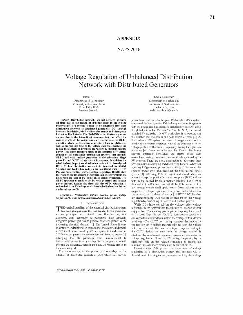
71

APPENDIX

NAPS 2016

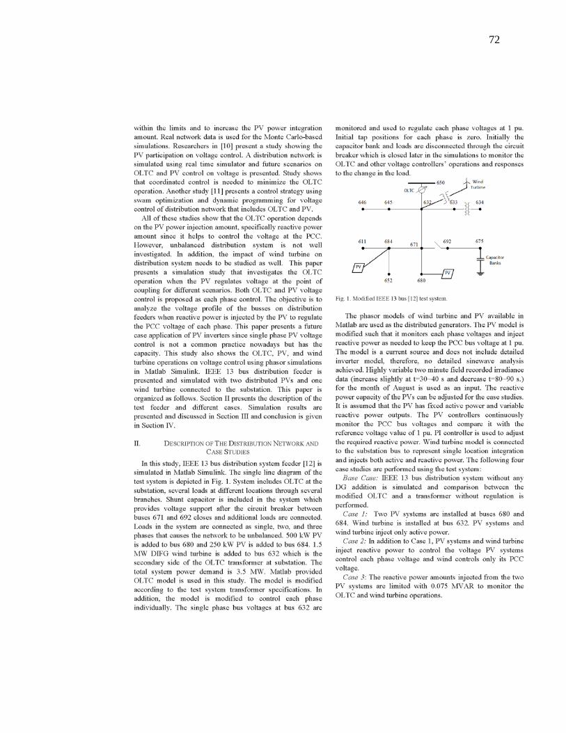
72

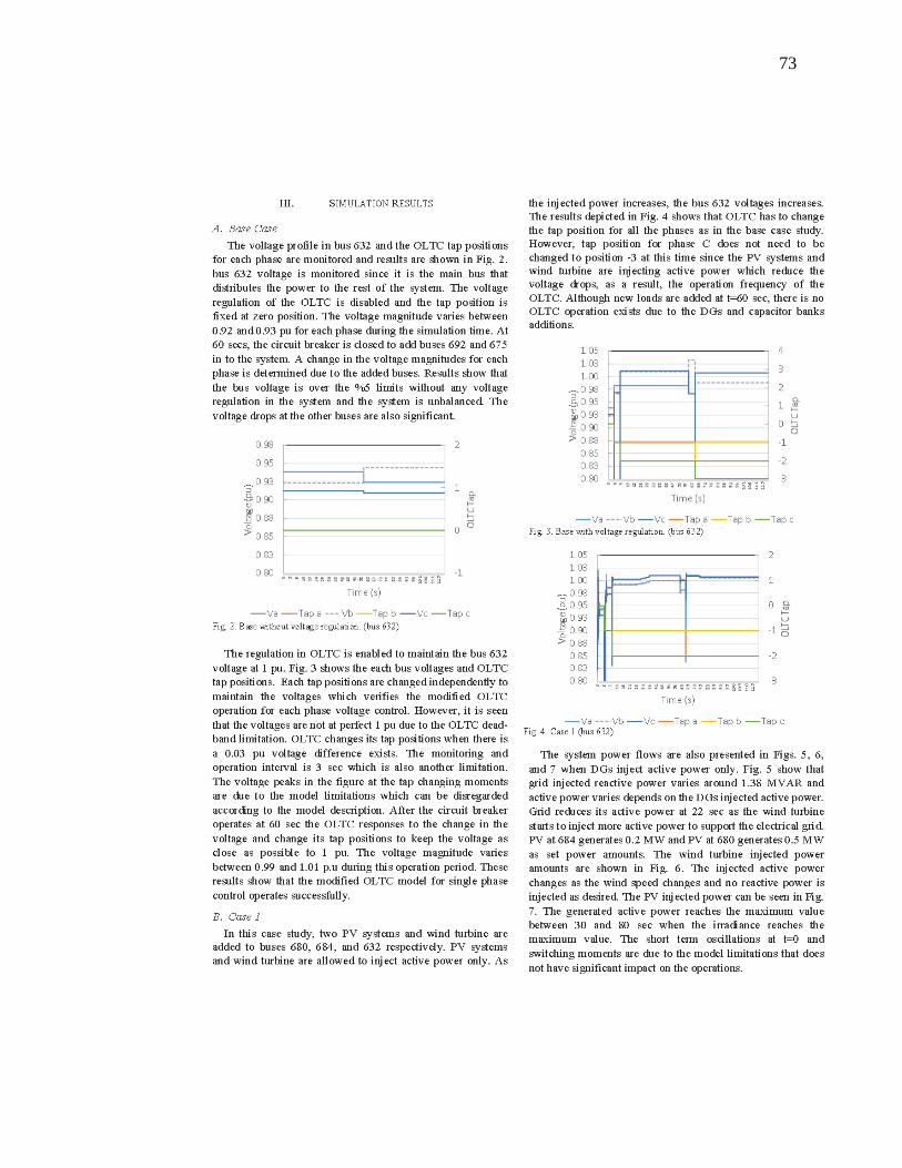
73

74

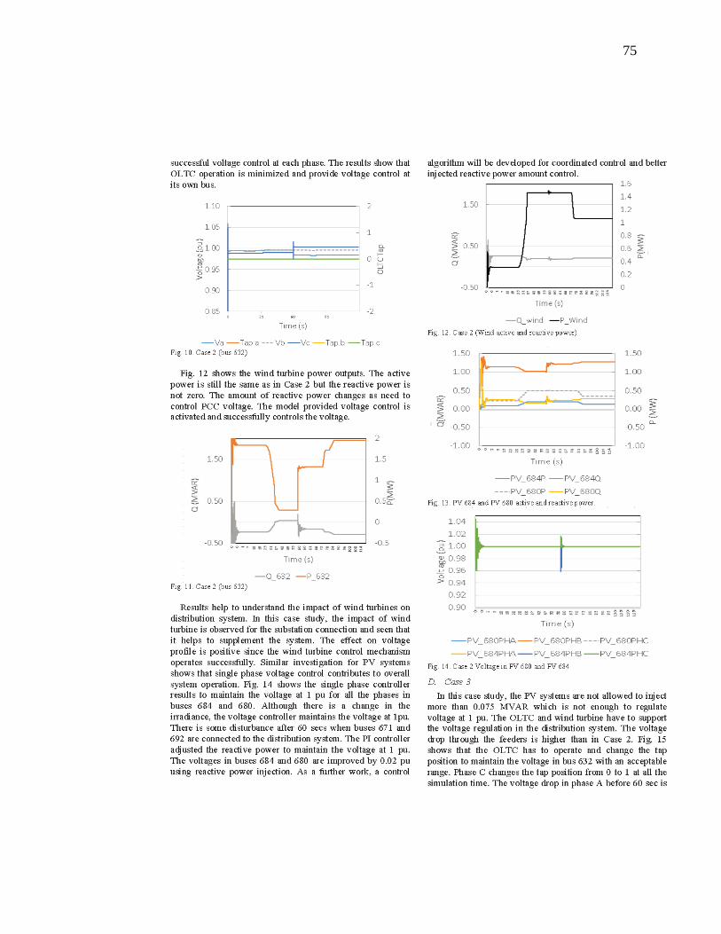
75

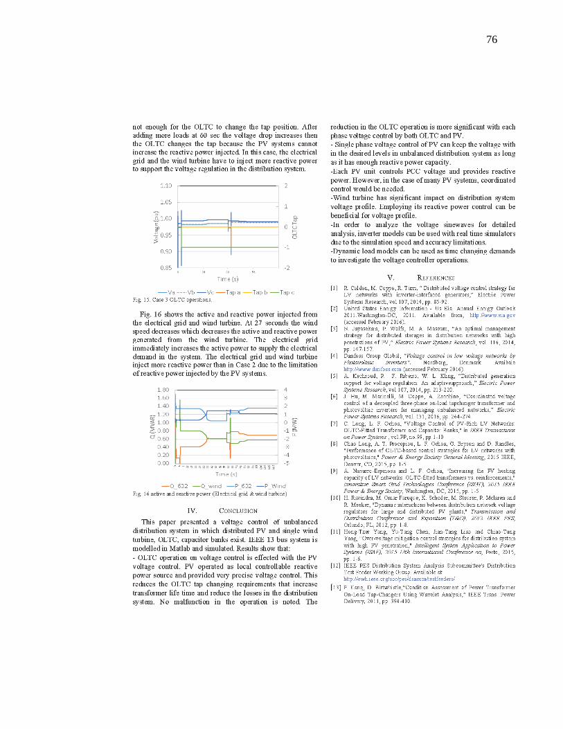
76

77

CASE 1 MAIN M FILE

function obj=OF(vecX) %Taking values from GA and assigning to value Tap=vecX(1); if Tap>0 set_param('A/OLTC','InitialTap','-1'); end if Tap<=0 set_param('A/OLTC','InitialTap','1'); end CapOnOff=vecX(2); QPV=vecX(3); %setting parameters on model with value from GA set_param('A/Constant','value',num2str(Tap)); set_param('A/Constant2','value',num2str(CapOnOff)); set_param('A/Constant3','value',num2str(QPV)); %Simulation and capturing the output simOut=sim('A','SaveOutput','on','OutputSaveName','values'); z=simOut.get('values'); Fvalues=z(:,1); Fvalues=Fvalues(end); % Setting up the obj function

obj=Fvalues; % (+) means min => CapOnOff=0 , (-) means max => CapOnOff=1..

end

CASE 1 PI PARAMETERS M FILE

function [ c, ceq ] = nlc( Vol ) %Simulation and capturing the output simOut=sim('A','SaveOutput','on','OutputSaveName','values'); z=simOut.get('values'); Voltage=z(:,2); Voltage=Voltage(end); % Setting up the obj function Vol(1)=Voltage;

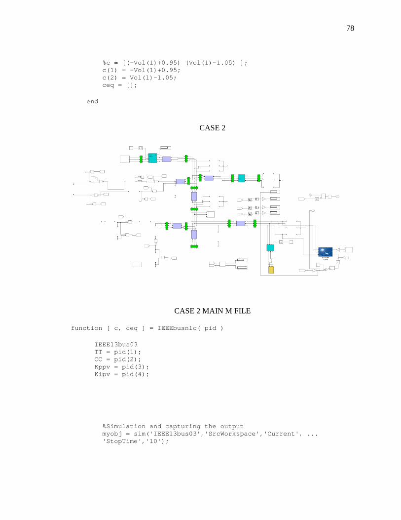
78

%c = [(-Vol(1)+0.95) (Vol(1)-1.05) ]; c(1) = -Vol(1)+0.95; c(2) = Vol(1)-1.05; ceq = []; end

CASE 2

CASE 2 MAIN M FILE

function [ c, ceq ] = IEEEbusnlc( pid ) IEEE13bus03 TT = pid(1); CC = pid(2); Kppv = pid(3); Kipv = pid(4); %Simulation and capturing the output myobj = sim('IEEE13bus03','SrcWorkspace','Current', ... 'StopTime','10');

79

c=zeros(length(myobj.yout),2); for i=1:1:length(myobj.yout) Vol=myobj.yout(i); c(i,1) = -Vol+0.95; c(i,2) = Vol-1.05; ceq =[]; end


function obj = IEEEbus(pid) TT = pid(1); CC = pid(2); Kppv = pid(3); Kipv = pid(4); if TT>0 set_param('IEEE13bus03/OLTC','InitialTap','-1'); end if TT<=0 set_param('IEEE13bus03/OLTC','InitialTap','1'); end myobj = sim('IEEE13bus03','SrcWorkspace','Current', ... 'StopTime','10'); obj=myobj.yout(end,2); end

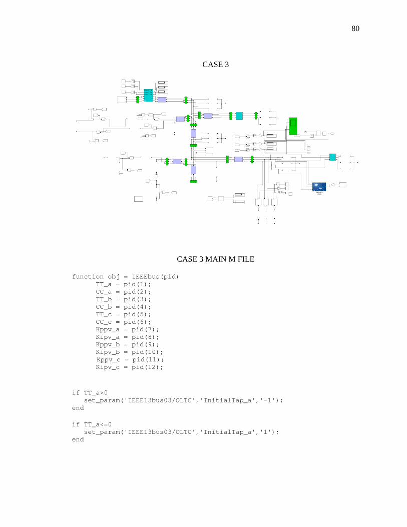
80

CASE 3

CASE 3 MAIN M FILE

function obj = IEEEbus(pid) TT_a = pid(1); CC_a = pid(2); TT_b = pid(3); CC_b = pid(4); TT_c = pid(5); CC_c = pid(6); Kppv_a = pid(7); Kipv_a = pid(8); Kppv_b = pid(9); Kipv_b = pid(10); Kppv_c = pid(11); Kipv_c = pid(12); if TT_a>0 set_param('IEEE13bus03/OLTC','InitialTap_a','-1'); end if TT_a<=0 set_param('IEEE13bus03/OLTC','InitialTap_a','1'); end

81

if TT_b>0 set_param('IEEE13bus03/OLTC','InitialTap_b','-1'); end if TT_b<=0 set_param('IEEE13bus03/OLTC','InitialTap_b','1'); end if TT_c>0 set_param('IEEE13bus03/OLTC','InitialTap_c','-1'); end if TT_c<=0 set_param('IEEE13bus03/OLTC','InitialTap_c','1'); end myobj = sim('IEEE13bus03','SrcWorkspace','Current', ... 'StopTime','10'); %0.05 obj=myobj.yout(end,1); end


function [ c, ceq ] = IEEEbusnlc( pid ) IEEE13bus03 TT_a = pid(1); CC_a = pid(2); TT_b = pid(3); CC_b = pid(4); TT_c = pid(5); CC_c = pid(6); Kppv_a = pid(7); Kipv_a = pid(8); Kppv_b = pid(9); Kipv_b = pid(10); Kppv_c = pid(11); Kipv_c = pid(12); %Simulation and capturing the output myobj = sim('IEEE13bus03','SrcWorkspace','Current', ... 'StopTime','10');

82

c=zeros(length(myobj.tout),6); for i=1:1:length(myobj.tout) Vola=myobj.yout(i+length(myobj.tout)); c(i,1) = -Vola+0.95; c(i,2) = Vola-1.05; Volb=myobj.yout(i+2*length(myobj.tout)); c(i,3) = -Volb+0.95; c(i,4) = Volb-1.05; Volc=myobj.yout(i+3*length(myobj.tout)); c(i,5) = -Volc+0.95; c(i,6) = Volc-1.05; ceq =[]; end end

CASE 4

83

CASE 4 MAIN M FILE

function [ c, ceq ] = IEEEbusnlc( pid ) IEEE13bus03 TT_a = pid(1); CC_a = pid(2); TT_b = pid(3); CC_b = pid(4); TT_c = pid(5); CC_c = pid(6); Kppv_a = pid(7); Kipv_a = pid(8); Kppv_b = pid(9); Kipv_b = pid(10); Kppv_c = pid(11); Kipv_c = pid(12); %Simulation and capturing the output myobj = sim('IEEE13bus03','SrcWorkspace','Current', ... 'StopTime','10'); c=zeros(length(myobj.tout),6); for i=1:1:length(myobj.tout) Vola=myobj.yout(i+length(myobj.tout)); c(i,1) = -Vola+0.95; c(i,2) = Vola-1.05; Volb=myobj.yout(i+2*length(myobj.tout)); c(i,3) = -Volb+0.95; c(i,4) = Volb-1.05; Volc=myobj.yout(i+3*length(myobj.tout)); c(i,5) = -Volc+0.95; c(i,6) = Volc-1.05; ceq =[]; end end

84


function obj = IEEEbus(pid) TT_a = pid(1); CC_a = pid(2); TT_b = pid(3); CC_b = pid(4); TT_c = pid(5); CC_c = pid(6); Kppv_a = pid(7); Kipv_a = pid(8); Kppv_b = pid(9); Kipv_b = pid(10); Kppv_c = pid(11); Kipv_c = pid(12); if TT_a>0 set_param('IEEE13bus03/OLTC','InitialTap_a','-1'); end if TT_a<=0 set_param('IEEE13bus03/OLTC','InitialTap_a','1'); end if TT_b>0 set_param('IEEE13bus03/OLTC','InitialTap_b','-1'); end if TT_b<=0 set_param('IEEE13bus03/OLTC','InitialTap_b','1'); end if TT_c>0 set_param('IEEE13bus03/OLTC','InitialTap_c','-1'); end if TT_c<=0 set_param('IEEE13bus03/OLTC','InitialTap_c','1'); end myobj = sim('IEEE13bus03','SrcWorkspace','Current', ... 'StopTime','10'); %0.05 obj=myobj.yout(end,1); end

Documents

Voltage regulation of unbalanced distribution network with