Weed Density Estimation from Digital Images in Spring Barley

Brian Bacher PedersenL9452

Department of Agricultural SciencesSection of AgroTechnology

The Royal Veterinary and Agricultural UniversityDK-2630 Taastrup, Denmark

November 2001

External supervisors:

Anne Mette WalterPreben Klarskov Hansen

Danish Institute of Agricultural SciencesDepartment of Crop ProtectionResearch Centre Flakkebjerg

Supervisors:

Bent S. BennedsenSimon Blackmore

Department of Agricultural SciencesSection of AgroTechnologyThe Royal Veterinary and Agricultural University

ii

ForordNærværende speciale er udarbejdet med henblik på erhvervelsen af den jordbrugsvidenskabeligekandidatgrad ved Den Kongelige Veterinær- og Landbohøjskole. Specialet er afleveret ved Institutfor Jordbrugsvidenskab – Sektion for Jordbrugsteknik. Specialet består af et artikel manuskript medhenblik på international publicering.

AcknowledgementThe author thanks Henning Nielsen for support and guidance in the development of the imageprocessing method and Spyros Fountas for great support in the phase of writing. The author alsothanks the people that helped in the data acquiring process and in the phase of analysing andwrithing. Furthermore, the author would like to thank the people in the section of AgriculturalTechnology at The Royal Danish Veterinary and Agricultural University for the hosting, as well asthe Department of Crop Protection at the Institute of Agricultural Sciences. Finally, a tanks toDorthe Kappel for her big patience.

Taastrup d. 7. november 2001

Brian Bacher Pedersen

iii

Table of contentsFORORD ..........................................................................................................................................................................IIACKNOWLEDGEMENT .....................................................................................................................................................IITABLE OF CONTENTS......................................................................................................................................................III

WEED DENSITY ESTIMATION FROM DIGITAL IMAGES IN SPRING BARLEY............................................1

ABSTRACT.......................................................................................................................................................................1INTRODUCTION ...............................................................................................................................................................1METHOD .........................................................................................................................................................................2

Field trial ...................................................................................................................................................................................... 2Image acquisition ......................................................................................................................................................................... 4Image processing.......................................................................................................................................................................... 4

Segmentation........................................................................................................................................................................... 4Detecting crop rows ................................................................................................................................................................ 5Crop/weed identification......................................................................................................................................................... 5

Statistics ....................................................................................................................................................................................... 7RESULTS .........................................................................................................................................................................9DISCUSSION AND CONCLUSIONS....................................................................................................................................15

Weed density .............................................................................................................................................................................. 15Image processing........................................................................................................................................................................ 16

REFERENCES .................................................................................................................................................................17REFERENCES TOTAL ......................................................................................................................................................19

1

Weed Density Estimation from Digital Images in Spring BarleyBy Brian Bacher Pedersen

AbstractA survey was carried out in a field of spring barley in 2000 with the objective of studying thepotential for weed density estimation by image processing, when increasing the row distance of thecrop. The number of weed plants was counted manually and estimated with the use of imageprocessing. Three different types of plots were established in 12, 24 and 36 cm row spacing. Eachplot consisted of two halves, one with crop and the other without, as a reference for the weeddensity potential. There were 45 plots for each of the three different plot types.

A method for weed density estimation by image processing was developed and the optimal rowdistance for image acquisition was found for two crop growth stages. The optimal crop row distancewas found to be 12 cm at leaf development stage and 36 cm at tillering stage. These row distancesmake image processing a possible method for weed density estimation in field, without makingchanges in the existing standards of field establishment.

By analysing the manually counted data it was found that the time for weed seedling emergencewas delayed because of the existence of spring barley. Reducing the crop row distance increased thedelayed effect.

IntroductionMost weed species have been found to be patchy distributed in agricultural fields (Rew & Cussans,1995). Therefore, uniform herbicide application across a whole field is unfavourable. Performingpatch spraying enables reduction of herbicide dosage (Christensen et al., 1999). Even though sitespecific weed management has been proved to have economic and environmental benefits(Lindquist et al., 1998), the success has been scanty in agriculture so far. This could be due to lackof equipment for performing site specific weed management.

For site specific weed management, two concepts have been introduced (Nordbo et al., 1994): Real-time concept – Weed monitoring and spraying carried out sequentially in the same

operation. The mapping concept – Weed monitoring and spraying carried out in separate operations.

The only real-time system, which has been used in small grain cereals, used an optoelectronicsensor for plant detection in the tramlines (Wartenberg & Dammer, 2001). The choice of herbicidehas to be decided before treatment. The mapping concept has the advantage to select a herbicidesolution that can manage the whole weed infestation in the field and the opportunity to validate theweed map before treatment. Thereby, the mapping concept seems to be the most realistic way ofperforming site specific weed management in small grain cereals in the near future.

Several approaches have been investigated for treatment map preparation. The basic parameters thathave been used in weed maps are weed cover and weed density. Weed density of the weed species,is used in the Decision Algorithm for Patch Spraying (DAPS) (Heisel et al., 1997). The algorithmcalculates the optimal herbicide and dose for each of the sampling points by using the speciescomposition. This was the reason for selecting weed density as the parameter to be estimated. The

2

species recognition was out of range for this project.

Crop often covers the weeds, which makes the separation of the crop from weed a difficult process(Thompson et al., 1990). It has been succeeded to estimate the weed density in spring barley withimage processing techniques (Benlloch & Rodas, 1998), by acquiring the images, when the cropwas in an early growth stage.

The best effect, of most herbicides, is obtained when the weed plants are still seedlings. Most yearsthis would be during the leaf development stage (Growth stage 10-19 (BBCH) (Lancashire et al.,1991)) of the crop. To overcome the problems due to overlapping leaves and dense canopy, anincrease of crop row spacing for better weed density estimation was introduced.

The aim of this project was to develop a simple image processing method that enables automaticweed density estimation for weed mapping in spring barley.

The hypothesis was that automatic weed density estimation in small grain cereals was possible bysimple image analysis if;1) the images were acquired before the crop had started tillering stage, or2) after tillering stage by increasing the cereal rows from 12 cm to 24 or 36 cm.

Method

Field trialThe experiment was conducted at the Danish Institute of Agricultural Sciences, Research CentreFlakkebjerg. The field (Sandy loam) with spring barley (Hordeum vulgare L. cv. Barke) wasestablished with three different row-spacings (12, 24 and 36 cm) and 38 plants per metre row(Figure 1), from a randomised plan (Figure 2).Each plot consisted of a 0.44x0.50 m crop area (A) and a 0.44x0.50 m crop-free area (B). The twoareas within the plot were photographed in two images (the frame and the plots are shown in Figure1).

A 3 m wide seed drill with 25 coulters was used and different row spacing was achieved bymanipulating the feed slides. The feed slides for coulter number 10-12 were closed for making thecrop free band and feed slides for coulter number 14-16 were manipulated to enable the three row-spacing. Each row-spacing was established for the entire track.Weeds in five plots were counted and photographed at each track with a 40 m distance, in a frameof 0.88x0.50 m. Figure 2 shows the distribution of the 135 plots (45 of each row-spacing).In the southern part of the field the samples were placed irregularly in relation to the rest of thefield, because the plots were mainly selected in order to have as much variation as possible in weeddensity.

3

1. Normal row spacing 12 cm (A) and a crop free band (B) on 44 cm.

3. Triple row spacing 36 cm (A) and a crop free band (B) on 44 cm.

0.50 m

0.44 m 0.44 m

0.50 m

0.44 m 0.44 m

0.50 m

0.44 m 0.44 m2. Double row spacing 24 cm (A) and a crop free band (B) on 44 cm.

Figure 1: Sketch of the three row-distances (12, 24 and 36 cm.) and the adjacent crop free area. Each plot consist oftwo parts (A and B). A frame of 0.88x0.50 metre was placed around the two areas. The frame was split in two halves,each of 0.44x0.50 metre.

12 cm 24 cm 36 cm

N

Figure 2: Illustration of the field with tramlines (dashed lines) and positions of the sampling points for the threecrop row-spacings.

4

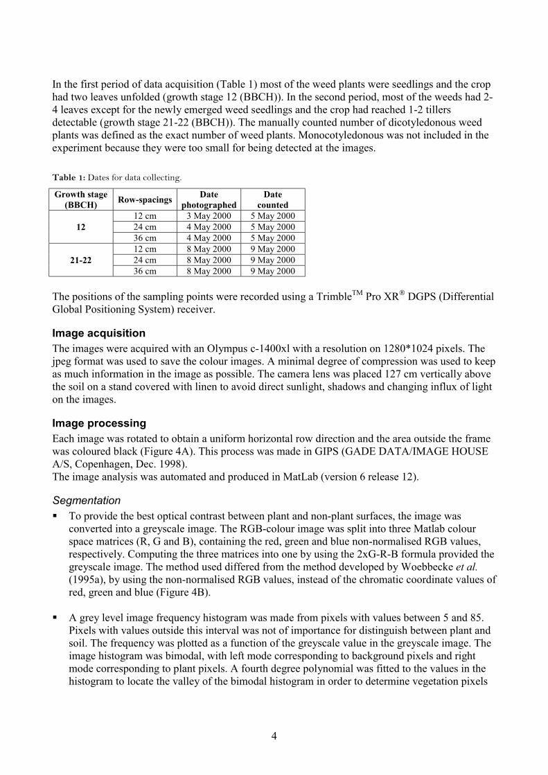
In the first period of data acquisition (Table 1) most of the weed plants were seedlings and the crophad two leaves unfolded (growth stage 12 (BBCH)). In the second period, most of the weeds had 2-4 leaves except for the newly emerged weed seedlings and the crop had reached 1-2 tillersdetectable (growth stage 21-22 (BBCH)). The manually counted number of dicotyledonous weedplants was defined as the exact number of weed plants. Monocotyledonous was not included in theexperiment because they were too small for being detected at the images.

Table 1: Dates for data collecting.

Growth stage(BBCH) Row-spacings Date

photographedDate

counted12 cm 3 May 2000 5 May 200024 cm 4 May 2000 5 May 20001236 cm 4 May 2000 5 May 200012 cm 8 May 2000 9 May 200024 cm 8 May 2000 9 May 200021-2236 cm 8 May 2000 9 May 2000

The positions of the sampling points were recorded using a TrimbleTM Pro XR DGPS (DifferentialGlobal Positioning System) receiver.

Image acquisitionThe images were acquired with an Olympus c-1400xl with a resolution on 1280*1024 pixels. Thejpeg format was used to save the colour images. A minimal degree of compression was used to keepas much information in the image as possible. The camera lens was placed 127 cm vertically abovethe soil on a stand covered with linen to avoid direct sunlight, shadows and changing influx of lighton the images.

Image processingEach image was rotated to obtain a uniform horizontal row direction and the area outside the framewas coloured black (Figure 4A). This process was made in GIPS (GADE DATA/IMAGE HOUSEA/S, Copenhagen, Dec. 1998).The image analysis was automated and produced in MatLab (version 6 release 12).

Segmentation To provide the best optical contrast between plant and non-plant surfaces, the image was

converted into a greyscale image. The RGB-colour image was split into three Matlab colourspace matrices (R, G and B), containing the red, green and blue non-normalised RGB values,respectively. Computing the three matrices into one by using the 2xG-R-B formula provided thegreyscale image. The method used differed from the method developed by Woebbecke et al.(1995a), by using the non-normalised RGB values, instead of the chromatic coordinate values ofred, green and blue (Figure 4B).

A grey level image frequency histogram was made from pixels with values between 5 and 85.Pixels with values outside this interval was not of importance for distinguish between plant andsoil. The frequency was plotted as a function of the greyscale value in the greyscale image. Theimage histogram was bimodal, with left mode corresponding to background pixels and rightmode corresponding to plant pixels. A fourth degree polynomial was fitted to the values in thehistogram to locate the valley of the bimodal histogram in order to determine vegetation pixels

5

stating at the right side of the valley. The circle is showing the lowest root for the curve and thisgreyscale value was used as threshold value (Figure 3A).

The threshold value was used in the greyscale image to make a binary image. Pixels with valueshigher than the threshold, are defined as plant pixels and are shown as white pixels (Figure 4C).

Detecting crop rows The frequency of the plant pixels was plotted in the crop row direction. Row positions were

determined after applying a low-pass filter to the resultant intensity curve to smoothen it (Olsen,1995) and then finding the absolute maxima in the curve defining the crop row centre (Figure3B).

Crop/weed identification All the solitary pixels were deleted to reduce the number of error objects. Dilation was made on

the image with a 9x9 matrix to connect adjacent objects. The objects, defining the leaves of thedicotyledonous weed plants were not connected, in the binary image, because the steamsconnecting them were not visible. This was the reason, for the weed seedlings to be detected astwo or more objects, in the binary image. Dilation was introduced to combine the belongingobjects. All the holes in the image objects were filled and the perimeters of the objects werecomputed (Figure 4D).

To find the number of weed plants, all objects in the image touching the line of pixels throughthe centre of the crop rows found in Figure 3B, were defined as crop plants. The image was splitinto sections between the rows. Filling the objects’ perimeters in the sections enabled thenumber of non-crop objects in the image to be defined (Figure 4E). The number of objects wasdefined as the number of weed plants in the image.

Figure 4E was used as a mask for counting the number of weed pixels in the binary image(Figure 4F).

0 50 100 150 200 250 3000

200

400

600

800

1000

1200

Row

num

ber i

n th

e im

age

Number of white pixels in the row

B

0 10 20 30 40 50 60 70 80 900

0.5

1

1.5

2

2.5

3

3.5x 10

4

Pixel value

Num

ber o

f pix

els

A

Figure 3: A) Image frequency histogram from the greyscale image. The circle is showing the lowest root for the curve,which is the threshold value used for binarisation of the image. B) Crop row positions were found (pluses) by adding a

6

A

C

E F

D

Figure 4: Step by step procedure of image processing. A) Rotation and border colouring of original image, B)Greyscale image made from 2xG-R-B, C) Binary image was made, D) Perimeter on dilated binary image, E) Weedpositions were found, F) Greyscale image showing crop (grey) and weed (white).

B

7

StatisticsFirst task was to find the number of weed plants in the image area was found. The number of weedplants found by image processing (No) (Figure 4E) was recalculated converted into (IP), which wasthe total number expected in the analysed area. The analysed number of pixels (Panalysed) was lessthan the number of pixels in the area of interest (PInterest). The number of pixels underneath the crop(Pcrop) was neither analysed for weed plants. It was assumed that the weed plants were evenlydistributed in the area of interest, and by this assumption equation (4) was made for ‘IP’.

( ) BPInterest −⋅= 10241280 (1)

weedplantcrop PPP −= (2)

Interestarea P

mP222.0= (3)

( )222.0 m

PPPNoIP

cropanalysedarea

⋅−⋅

= (4)

No -is the number of weed plants detected by image processing.B -is the number of pixels coloured black around the area of interest in

the image (border).PInterest -is the number of pixels inside the frame in the image (equation (1)).Pplant -is the number of plant pixels found in the area of interest.Pweed -is the number of pixels found in the objects detected as weed.Pcrop -is the number of pixels found to be crop (equation (2)).Parea -is the area of each pixel in the image measured in m2 (equation (3)).Panalysed -is the number of pixels inside PInterest analysed for number of weed

plants (Panalysed is less than PInterest).IP -is the number of weed plants found in the frame by image

processing with subject to the analysed area (equation (4)).1280⋅1024 -is the number of image pixels.

All data were logarithm transformed to approximate a normal distribution. Bartlett tests for variancehomogenity was used. The MIXED procedure in SAS version 8 was used for data analysis (SASInstitute Inc., 1994).

Equation (5) was used to test if the number of weed plants was the same in the crop area and in therelated crop free area.

( ) εαµ ++++++= dttggtp GFEDLn mdW (5)

Symbols: p (point) = a (crop area) ; b (crop free area)t (tramline) = 1, 2,…, 9g (repetition) = 1, 2,…, 5d (row distance) = 1 (12cm); 2 (24cm); 3 (36cm)Wmd the manually counted weed density (n=270).µ the estimated mean value.α the systematic effect (the factor to be examined).

8

D, E, F, G the random effects are included to take the field variation intoaccount.

ε error.

Equation (6) was used to test if the number of weed plants was the same in the three different rowdistances. The number of weed plants counted in the crop area was used as co-variant to take theweed density potential into account in the analysis of the three row-spacing. This was necessarybecause of a varied weed distribution in the field particularly caused by weed experiments in thefield in the previous years.

( ) ( ) εα +++++⋅= dttggtmcddmcfd GFEDWLnWLn (6)

Symbols: d (row distance) = 1 (12cm); 2 (24cm); 3 (36cm)t (tramline) = 1, 2,…, 9g (repetition) = 1, 2,…, 5Wmcfd the weed density found by manual weed counting in the crop free

area (n=135).Wmcd the weed density found by manual weed counting in the crop area

next to the crop free area (n=135).α the systematic effect (the factor to be examined).D, E, F, G the random effects are included to take the field variation into

account.ε error.

Equation (7) was used to test if the number of weed plants was the same when the weed density wasfound by manual weed counting and by image processing

( ) εαµ ++++++= dttggtmd GFEDWLn (7)

m (method) = 1(manual counting); 2(Image Processing)t (tramline) = 1, 2,…, 9g (repetition) = 1, 2,…, 5d (row distance) = 1 (12cm); 2 (24cm); 3 (36cm)Wd the weed density found by manual weed counting and image

processing (n=540).µ the estimated mean value.α, β the systematic effects (the factors to be examined).D, E, F, G the random effects are included to take the field variation into

account.ε error.

Equation (8) was used to find linear relation between the number of weed plants that was manuallycounted and found by image processing. Linearity was tested for the row distances (12, 24, 36 and44 cm). The 44 cm row distance was originally the crop free area.

( ) ( ) εβα ++++⋅+= tggtipdrrmd FEDWLnWLn (8)

9

r (row distance) = 1 (12cm); 2 (24cm); 3 (36cm); 4 (44cm)t (tramline) = 1, 2,…, 9g (repetition) = 1, 2,…, 5Wmd the weed density found by manual weed counting (n=270).Wipd the weed density found by image processing (n=270) (Wipd=IP).α, β the systematic effects (the factors to be examined).D, E, F, G the random effects are included to take the field variation into

account.ε error.

Each of the equations 5-8 was used for analysing BBCH 12 and 22 respectively.

ResultsIn the crop free areas there were significantly more weed seedlings than in the crop areas at growthstage 12 (BBCH) and there was a tendency for the same at growth stage 22 (BBCH) (Table 2). Thisindicated that the crop had a reducing influence on the weed density (Wmd), and this influence wasincreased at the early growth stage.

Table 2: Estimates (Wmd), standard error and significance levels for crop area and crop free area, when the number ofweed plants was counted at two growth stages.

Growth stage(BBCH) Crop Estimate

(Ln(Wmd))Standard

Error Pr>|t| Sign.

+ 3.138112 - 3.2573 0.1486 0.0274 *

+ 3.314022 - 3.4085 0.1582 0.0603 (NS)

The same analysis was made for each of the three row distances (12, 24 and 36 cm) at the twogrowth stages (Table 3). At growth stage 12 (BBCH) the biggest difference was found at 12 cm rowdistance and the smallest at 36 cm. This indicated that increasing row distance at the early growthstage decreased the reducing effect.From the estimates shown in Table 3 it can be seen that the weed density (Wmd) increased from theearly to the late growth stage. In the same period the difference between the areas with and withoutcrop decreased. The germination of the weeds had not finished at the time of the first counting. Thetime for emergence of weed seedlings was in this experiment depending on the row distance of cropplants in the field.

The crop free area was used as a co-variant to take the weed density potential into account in theanalysis of the number of weed plant counted in the plots from the three row distances. This wasnecessary because of a varying weed distribution in the field presumably caused by weedexperiments in the field previous years.The weed density counted in the crop area (Wmcd) against the density in the crop free area (Wmcfd)for the two crop growth stages 12 and 22 (BBCH) is illustrated in Figure 4A and 4B. The weeddensity in the crop free area (Wmcfd) was about 18% (12 cm), 8% (24 cm) and 4% (36 cm) higherthan the density in the crop area (Wmcd). At growth stage 22 (BBCH) the weed density was about6% (12 cm), 0% (24 cm) and 12% (36 cm) higher in the crop free area (Wmcfd) than in the crop area(Wmcd).

10

Figure 5: The back transformed relations are illustrated for the number of weed plants per m2 counted in the cropfree area against the number of weed plants per m2 counted in the crop area for (A) growth stage 12 (BBCH) and (B)growth stage 22 (BBCH).

RowSpacing 12cm 24cm 36cm

0

100

200

300

400

500

Num

ber o

f wee

d pl

ants

per

m2 in

cro

p fr

ee a

rea

RowSpacing 12cm 24cm 36cm

Number of weed plants per m2 in crop area

0

100

200

300

400

500

0 50 100 150 200 250 300 350 400 450

A

B

11

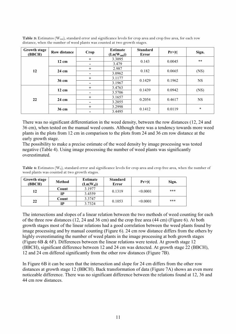
Table 3: Estimates (Wmd), standard error and significance levels for crop area and crop free area, for each rowdistance, when the number of weed plants was counted at two growth stages.

Growth stage(BBCH) Row distance Crop Estimate

(Ln(Wmd))Standard

Error Pr>|t| Sign.

+ 3.309512 cm - 3.479 0.143 0.0045 **

+ 2.98724 cm - 3.0962 0.182 0.0665 (NS)

+ 3.1177

12

36 cm - 3.1967 0.1429 0.1962 NS

+ 3.476312 cm - 3.5706 0.1439 0.0942 (NS)

+ 3.165724 cm - 3.2055 0.2054 0.4617 NS

+ 3.2998

22

36 cm - 3.4495 0.1412 0.0119 *

There was no significant differentiation in the weed density, between the row distances (12, 24 and36 cm), when tested on the manual weed counts. Although there was a tendency towards more weedplants in the plots from 12 cm in comparison to the plots from 24 and 36 cm row distance at theearly growth stage.The possibility to make a precise estimate of the weed density by image processing was testednegative (Table 4). Using image processing the number of weed plants was significantlyoverestimated.

Table 4: Estimates (Wd), standard error and significance levels for crop area and crop free area, when the number ofweed plants was counted at two growth stages.

Growth stage(BBCH) Method Estimate

(Ln(Wd))Standard

Error Pr>|t| Sign.

Count 3.197712 IP 3.4559 0.1319 <0.0001 ***

Count 3.374722 IP 3.7324 0.1053 <0.0001 ***

The intersections and slopes of a linear relation between the two methods of weed counting for eachof the three row distances (12, 24 and 36 cm) and the crop free area (44 cm) (Figure 6). At bothgrowth stages most of the linear relations had a good correlation between the weed plants found byimage processing and by manual counting (Figure 6). 24 cm row distance differs from the others byhighly overestimating the number of weed plants in the image processing at both growth stages(Figure 6B & 6F). Differences between the linear relations were tested. At growth stage 12(BBCH), significant difference between 12 and 24 cm was detected. At growth stage 22 (BBCH),12 and 24 cm differed significantly from the other row distances (Figure 7B).

In Figure 6B it can be seen that the intersection and slope for 24 cm differs from the other rowdistances at growth stage 12 (BBCH). Back transformation of data (Figure 7A) shows an even morenoticeable difference. There was no significant difference between the relations found at 12, 36 and44 cm row distances.

12

Figure 6: Logarithm transformed number of weed plants counted in the field (Wmd) as a function of the logarithmtransformed number of weed plants found by image processing (Wipd). A-D shows the functions for growth stage 12(BBCH) where A is 12 cm, B is 24 cm C is 36 cm and D is 44 cm or the crop free area. E-H shows the functions forgrowth stage 22 (BBCH) where E is 12 cm, F is 24 cm G is 36 cm and H is 44 cm or the crop free area. α is theintersection and β the slope of the functions.

C

0

1

2

3

4

5

0

1

2

3

4

5

0

1

2

3

4

5

0

1

2

3

4

5

1 2 3 4 5 1 2 3 4 5

Log

(Num

ber o

f wee

d pl

ants

cou

nted

in th

e fie

ld)

Log (Number of weed plants found by image processing)

RowSpacing 12cm 24cm 36cm 44cm

A B

D

E F

G H

α: −0.32β: 1.04

α: −1.91β: 1.46

α: −0.37β: 1.04

α: −0.11β: 0.96

α: 2.63β: 0.24

α: −1.24β: 1.19

α: −0.09β: 0.92

α: −0.17β: 0.94

13

Figure 7: Back transformed number of weed plants counted in the field as a function of the number of weed plantsfound by image processing. Growth stage 12 (BBCH) (A) and growth stage 22 (BBCH) (B).

At growth stage 22 (BBCH), 12 cm row distance was not suitable for image processing because of alarge crop covered area. There was no relation between the weed density found by image processing(Wmd) and the density manually counted in the field (Wmd) (Figure 6E & 7B). The confidence limitfor each of the row distances is shown in Figure 8. At the early growth stage (Figure 8A) the errorin estimates was ±10-15 weed plants depending on the row distance, when 150 weed plants per m2

were found by image processing. At the late stage (Figure 8B) the error in estimates increased to

0

100

200

300

400

500

0

100

200

300

400

500

0 100 200 300 400

RowSpacing 12cm 24cm 36cm 44cm

Number of weed plants per m2 found by image processing

Num

ber o

f wee

d pl

ants

per

m2 c

ount

ed in

the

field

A

B

14

±17-21 plants, when 12 cm was eliminated.

Figure 8: The maximal error in estimates using image processing for weed density estimation at growth stage 12 (A)and 22 (B) (BBCH). The error in estimates was the 95% confidence limit found for the counted weed density as afunction of the density found by image processing.

0

50

100

150

RowSpacing 12cm 24cm 36cm 44cm

0

50

100

0 50 100 150 200 250 300 350 400 450

Number of weed plants per m2 found by image processing

Erro

r in

estim

ates

(Num

ber o

f wee

d pl

ants

per

m2 )

A

B

15

Discussion and conclusions

Weed densityIt was assumed that there was the same weed density potential in the two frame halves, one withcrop and one without. The number of germinating weed seedlings was supposed to be equal in thetwo areas, as they were exposed to the same cultivation, because mechanical disturbance of the soilstimulates the germination (Håkansson, 1999).The number of weed plants, which were manually counted, in the crop free area, were significantlylarger than in the crop area when the crop was at growth stage 12 (BBCH). Spring barley has beenbred for fast germination and emergence. As a consequence of the fast crop germination andemergence, changes in nutrient and water content of the soil, could induce dormancy in the weedseeds (Zimdahl, 1999). Moreover, the lower number of weed plants in the crop area can be due toallelochemicals from the root exudates of spring barley (Baghestani et al., 1999).In the crop area the weed density was depending on the crop row distance. That indicated that thecrop had a reducing effect on the number of weed plants. The weed density was higher at rowdistance 36 cm and reducing accordingly to 12 cm. This effect was distinct at the early growthstage. At the late growth stage the inhibiting effect on the weed density declined, indicating that thecrop plants inhibited the time for weed seedling germination and not the total number ofgerminating seedlings.

There were linear relations between the logarithm transformed weed density found by imageprocessing and density found by manual weed counting, proving that image processing could beused for weed density estimation.

At crop growth stage 12 (BBCH), the optimal row distance for weed density estimation by imageprocessing was found to be 12 cm. The error in estimates (Number of weed plants per m2) wasalmost equal for the different row distances, until the number of weed plants exceeded 200 per m2.At that level, 44 cm row distance was more precise. 36 cm row distance was almost equal to 12 cm.At growth stage 22 (BBCH), the weed density estimation at 36 cm row distance was found to bealmost as good as estimation at 44 cm. This result gave no reason for increasing the row distancefrom 36 to 44 cm.

The normal width of the tramlines in small grain cereals is 36 cm, which was found to be theoptimal distance for weed density estimation at growth stage 22 (BBCH). If the tramlines could beused for estimating the weed density it would increase the opportunity of making the systemcommercial. In practical farming, crop free bands cannot easily be accepted. Implementing thesystem would be easier if the tramlines could be used for image acquisition, instead of using cropfree areas.The problem in using the tramlines is that the weed population has been found to be different fromthe population in rest of the field (Walter, 1994). The difference in the weed population could bedue to the increased row distance, but it could also be due to compaction of the soil. Otherinvestigations found that the weed density in the tramlines and in the neighbouring plant stand wascomparable to the time for herbicide application in winter crops (Petry, 1989). Therefore, if theweed density is comparable in spring crops, at the time for herbicide application, the tramlinescould be used for weed density estimation, but further investigations is needed to test this idea.

16

Image processingImages were acquired with a normal digital camera with a relative low resolution yielding imageswith a reasonably high level of information. However, using a camera with higher resolution, or a 3CCD camera, would considerably increase the information. By changing the compressed jpeg fileformat to a non-compressed format, the loss of information would be negligible.

The binarisation resulted frequently in weed plants being subdivided in individual objects. Dilationwas used to connect these objects. However, the matrix used was too small to connect all theobjects, but a larger matrix would merge objects not belonging to the same plant and a non-desirable underestimation would appear. The number of leaves increased by the age of the weedplants, and thereby the number of objects to be overestimated.

If the image processing method, suggested in this paper, is to be introduced to agriculture, somefurther research has to be made. The weed density and weed population in the tramlines has to befurther examined and explained. The error of weed estimates in the image processing has to beevaluated if it is acceptable, or it has to be improved.

Reducing the error of estimates calls for the image processing to be further developed. This couldbe done by improving the procedure that connects objects belonging to the same plant in the binaryimage. Further, the thresholding procedure for binarisation could be improved as suggested byPérez et al. (2000), a method to ensure all plant pixels in the image are detected. If the weed plantsin the images are still detected as more than one object, a method for detecting connected segmentscould be introduced (Andreasen et al., 1997). Furthermore, shape features could be implemented fordetecting the weed plants (Woebbecke et al., 1995b).

When a precise estimation of weed plants has been achieved, an implementation with weed speciesrecognition would lead to an automated weed species density detection system in small graincereals.

17

References

Andreasen C; Rudomo, M; Sevestre, S. Assessment of weed density at an early stage by use ofimage processing. Weed Research 1997, 37, 5-18

Baghestani A; Lemieux, C; Leroux, G D; Baziramakenga, R; Simard, R R. Determination ofallelochemicals in spring cereal cultivars of different competitiveness. Weed Science 1999,47(5), 498-504

Benlloch J V ; Rodas, A. Dynamic model to detect weeds in cereals under actual field conditions.Proceedings of SPIE1998, 3543, 302-310

Christensen S; Walter, A M; Heisel, T. The patch treatment of weeds in cereals. Brighton CropProtection Conference - Weeds 1999, 591-600

Heisel T; Christensen, S; Walter, A M. Validation of weed patch spraying in spring barley –Preliminary trial. Precision Agriculture ’97 1997, 879-886

Håkansson S. Soil tillage and weeds on arable land. Chapter 21 in: Weed Science Compendium.Copenhagen: DSR Forlag, 1999, 359-396

Lancashire P D; Bleiholder, H; Van den Boom, T; Langelüddeke, P; Strauss, R; Weber, E;Witzenberger, A. A uniform decimal code for the growth stages of crops and weeds.Annals of Appleid Biology 1991, 119, 561-601

Lindquist J L; Dieleman, J A; Mortensen, D A; Johnson, G A; Wyse, P D. Economicimportance of managing spatially heterogeneous weed populations. Weed Technology 1998,12(1), 7-13

Nordbo E; Christensen, S; Kristensen, K; Walter, M. Patch spraying of weed in cereal crops.Aspects of Applied Biology 1994, 40, 325-334

Olsen H J. Determination of row position in small-grain crops by analysis of video images.Computers and Electronics in Agriculture 1995, 12, 147-162

Petry W. Unkrautkontrolle im landwirtschaftlichen Pflanzenbau mit Hilfe der quantitativenBildanalyse. Dissertation, Universität Bonn, 1989, 1-74

Pérez A J; López, F; Benlloch, J V; Christensen, S . Colour and shape analysis techniques forweed detection in cereal fields. Computers and Electronics in Agriculture 2000, 25, 197-212

Rew L J ; Cussans, G W. Patch ecology and dynamics - how much do we know? Brighton cropprotection conference: weeds 1995, 3, 1059-1068

SAS Institute Inc. SAS/STAT User's Guide. North Carolina: SAS Institute,1994.

Thompson J F; Stafford, J V; Ambler, B. Weed detection in cereal crops. ASAE Paper No.89-7512.St.Joseph, Mich.: ASAE. 1990

18

Walter A M. Gradueret Ukrudtsbekæmpelse: Registrering og Kortlægning af Ukrudt. Master thesisin weed science at The Royal Veterinary and Agricultural University. 1994, 1-62

Wartenberg G ; Dammer, K-H. Site-Specific Real Time Application of Herbicides in Practice.Precision Agriculture '01 2001, 617-622

Woebbecke D M; Meyer, G E; Bargen, K v; Mortensen, D A; Von-Bargen, K. Color indices forweed identification under various soil, residue, and lighting conditions. Transactions of theASAE 1995a, 38(1), 259-269

Woebbecke D M; Meyer, G E; Von Bargen, K; Mortensen, D A . Shape features for identifyingyoung weeds using image analysis. Transactions of the ASAE 1995b, 38(1), 271-281

Zimdahl R L. Weed biology: Reproduction and despersal. Chapter 3 in: Weed ScienceCompendium. Copenhagen: DSR Forlag, 1999, 27-56

19

References total

Ahmad U; Kondo, N; Arima, S; Monta, M; Mohri, K. Weed Detection in Lawn Field Based on Gray-ScaleUniformity. Environmental Control in Biology 1998, 36(4), 227-237

Andersen H J; Onyango, C M; Marchant, J A. The Design and Operation of an Imaging Sensor for DetectionVegetation. International Journal Imaging Systems and Technology 2000, 11(2), 144-151

Andersen H J ; Granum, E. Classifying Illumination Condition from Two Light Sources by Colour HistogramAssessment. Journal of Optical Society of America A 2000, 17(4), 667-676

Andreasen C; Rudomo, M; Sevestre, S. Assessment of weed density at an early stage by use of image processing.Weed Research 1997, 37, 5-18

Audsley E ; Beaulah, A. Combining weed maps to produce a treatment map for patch spraying. Aspects of AppliedBiology 1996, 46, 111-118

Baghestani A; Lemieux, C; Leroux, G D; Baziramakenga, R; Simard, R R. Determination of allelochemicals inspring cereal cultivars of different competitiveness. Weed Science 1999, 47(5), 498-504

Ballaré C L ; Casal, J J. Light signals perceived by crop and weed plants. Field Crops Research 2000, 67, 149-160

Bartlett M S. Fitting a straight line when both variables are subject to error. Biometrics 1949, 5, 207-212

Bell T. Automatic tractor guidance using carrier-phase differential GPS. Computers and Electronics in Agriculture2000, 25, 53-66

Benlloch J V; Heisel, T; Christensen, S; Rodas, A. Image Processing Techniques for Determination of Weeds inCereal. Bio-Robotics'97: Sensors and Automatic Decision, 1997, 195-200

Benlloch J V ; Rodas, A. Dynamic model to detect weeds in cereals under actual field conditions. Proceedings of theSPIE 1998, 3543, 302-310

Bennedsen B S ; Guiot, M. Estimation of plant density from aerial red-near infrared images and interaction with weedsinfestation and soil variability. Precision Agriculture '01 2001, Part A, 145-150

Biller R H. Reduced Input of Herbicides by Use of Optoelectronic Sensors. Journal of Agricultural EngineringResearch 1998, 71, 357-362

Birdsall J L; Quimby Jr., P C; Rees, N E; Svejcar, T J; Sowell, B F. Image Analysis of Leafy Spurge (Euphorbiaesula) Cover. Weed Technology 1997, 11, 798-803

Blackshaw R E; Molnar, L J; Chervalier, D F; Lindwall, C W. Factors affecting the operation of the weed-sensingDetectspray system. Weed Science 1998, 46, 127-131

Blasco J; Benlloch, J V; Agusti, M; Molto, E. Machine Vision for Precise Control of Weeds. Proceedings of the SPIE1998, 3543, 336-343

Bleiholder H; Weber, E; Van den Boom, T; Hack, H; Witzenberger, A; Lancashire, P D; Langelüddeke, P;Strauss, R. A New Uniform Decimal Code for the Growth Stages of Crops and Weeds. Brighton CropProtection Conference - Pest & Diseases 1990, 667-672

Brown R B; Steckler, P G A; Anderson, G W. Remote Sensing for Identification of Weeds in No-till Corn.Transactions of the ASAE 1994, 37(1), 297-302

20

Burks T F; Shearer, S A; Payne, F A. Classification of Weed Species Using Color Texture Features and DiscriminantAnalysis. Transactions of the ASAE 2000, 43(2), 441-448

Carroll R J ; Ruppert, D. Transformation and Weighting in Regression. New York: Chapman and Hall, 1988.

Chapron M; Requena-Esteso, M; Boissard, P; Assemat, L. A method for recognizing vegetal species frommultispectral images. Precision Agriculture ’99, 1999, 239-247

Chapron M; Boissard, P; Assemat, L. A method for 3D reconstuction of vegetation by stereovision. PrecisionAgriculture ’99, 1999, 249-256

Christensen S ; Nordbo, E. Weed cover mapping with spectral reflectance measurements. Aspects of Applied Biology1994, 37, 171-179

Christensen S; Heisel, T; Walter, A M. Patch spraying in cerals. Second International Weed Control Congress,Copenhagen 1996, 963-968

Christensen S ; Heisel, T. Patch spraying using historical, manual and real time monitoring of weeds in cereals.Zeitschrift für Pflanzenkrankheiten und Pflanzenschutz, Sonderheft XVI 1998, 16 (XVI), 257-263

Christensen S; Heisel, T; Benlloch, J V. Patch spraying and rational weed mapping in cereals. Proceedings of the 4thInternational Conference on Precision Agriculture. Minnesota 1998, 773-785

Christensen S ; Heisel, T. Digitalt kamerasystem til detektion af ukrudt. DJF-Rapport 1998, 15. DanskePlanteværnskonference - Sygdomme og skadedyr 3, 161-171

Christensen S; Walter, A M; Heisel, T. The patch treatment of weeds in cereals. Brighton Crop Protection Conference- Weeds 1999, 591-600

Dieleman J A; Mortensen, D A; Buhler, D D; Cambardella, C A; Moorman, T B. Identifying associations amongsite properties and weed species abundance. I. Multivariate analysis. Weed Science 2000, 48(5), 567-575

Dieleman J A; Mortensen, D A; Buhler, D D; Ferguson, R B . Identifying associations among site properties andweed species abundance. II. Hypothesis generation. Weed Science 2000, 48(5), 576-587

Doruchowski G; Jaeken, P; Holownicki, R. Target detection as a tool of selective spray application on trees andweeds in orchards. Proceedings of SPIE 1998, 3543, 290-301

El-Faki M S; Zhang, N; Peterson, D E. Factors affecting color-based weed detection. Transactions of the ASAE2000, 43(4), 1001-1009

El-Faki M S; Zhang, N; Peterson, D E. Weed detection using color machine vision. Transactions of the ASAE 2000,43(6), 1969-1978

Esau K. The Seed. Chapter 23 in: Anatomy of Seed Plants. John Wiley & Sons, 1977, 2nd Edition(23), 455-473

Fan G; Zhang, N; Peterson, D E; Loughin, T M; Fan, G; Zhang, N Q. Real-time weed detection using machinevision. ASAE Paper no. 983032. Orlando, Florida: ASAE. 1998.

Favier J; Ross, D W; Tsheko, R; Kennedy, D D; Muir, A Y; Fleming, J. Discrimination of weeds in brassica cropsusing optical spectral reflectance and leaf texture analysis. Proceedings of the SPIE 1998, 3543, 311-318

Felton W L ; McCloy, K R. Spot spraying -Microprocessor-controlled, weed-detecting technology helps save moneyand the environment. Agricultural Engineering 1992, 73(6), 9-12

Feyaerts F; Pollet, P; Van Gool, L; Wambacq, P. Vision system for weed detection using hyper-spectral imaging,structural field information and unsupervised training sample collection. The 1999 Brighton Conference -

21

Weeds 1999, 2, 607-614

Feyaerts F; Pollet, P; Van Gool, L; Wambacq, P. Hyperspectral image sensor for weed selective spraying.Proceedings of SPIE 1999, 3897, 193-203

Gerhards R; Nabout, A; Sökefeld, M; Kühbauch, W; Nour Eldin, H A. Automatische Erkennung von zehnUnkrautarten mit Hilfe digitaler Bildverarbeitung und Fouriertransformation. Journal of Agronomy and CropScience 1993, 171, 321-328

Gerhards R; Sökefeld, M; Knuf, D; Kühbauch, W. Kartierung und geostatistische Analyse der Unkrautverteilung inZuckerrübenschlägen als Grundlage für eine teilschlagspezifische Bekämpfung. Journal of Agronomy andCrop Science 1996, 176, 259-266

Gerhards R; Sökefeld, M; Schulze, L K; Mortensen, D A; Kuhbauch, W. Site specific weed control in winterwheat. Journal of Agronomy and Crop Science 1997, 178(4), 219-255

Gerhards R; Sökefeld, M; Kühbauch, W. Einsatz der digitalen Bildverarbeitung bei der teilschlagspezifischenUnkrautkontrolle. Zeitschrift für Pflanzenkrankheiten und Pflanzenschutz, Sonderheft XVI 1998, 273-278

Ghersa C M; Benech-Arnold, R L; Satorre, E H; Martínez-Ghersa, M A. Advances in weed managementstrategies. Field Crops Research 2000, 67, 95-104

Haggar R J; Stent, C J; Isaac, S. A Prototype Hand-held Patch Sprayer for Killing Weeds, Activated by SpectralDifferences in Crop/Weed Canopies. Journal of Agricultural Enginering Research 1983, 28(4), 349-358

Haggar R J; Stent, C J; Rose, J. Measuring spectral differences in vegetation canopies by a reflectance ratio meter.Weed Research 1984, 24, 59-65

Hague T ; Tillett, N D. A bandpass filter-based approach to crop row location and tracking. Mechatronics 2001, 11(1),1-12

Hanks J E ; Beck, J L. Sensor-Controlled Hooded Sprayer for Row Crops. Weed Technology 1998, 12, 308-314

Hansen P K ; Christensen, S. Using image analysis to determine the early growth habit of cereals. Proceedings 11thEWRS Symposium 1999, 117-117

Heisel T; Andreasen, C; Ersbøll, A K. Annual weed distributions can be mapped with kriging. Weed Research 1996,36, 325-337

Heisel T; Christensen, S; Walter, A M. Weed Managing Model for Patch Spraying in Cereal. Proceedings of theThird International Conference on Precision Agriculture. Minneapolis, Minnesota, USA. 1996, 999-1007

Heisel T; Christensen, S; Walter, A M. Validation of weed patch spraying in spring barley – Preliminary trial.Precision Agriculture ’97 1997, 879-886

Heisel T; Christensen, S; Walter, A M. Ukrudtskort og pletsprøjtning. DJF-Rapport 1998, 15. DanskePlanteværnskonference - Sygdomme og skadedyr 3, 151-160

Heisel T ; Christensen, S. A Digital Camera System for Weed Detection. Proceedings of the Fourth InternationalConference on Precision Agriculture. Madison: USA. 1999, 1569-1577

Heisel T; Christensen, S; Walter, A M. Whole-Field Experiments with Site-Specific Weed Management. PrecisionAgriculture ’99. 1999, 759-768

Heisel T; Ersbøll, A K; Andreasen, C. Weed Mapping with Co-Kriging Using Soil Properties. Precision Agriculture1999, 1(1), 39-52

22

Hemming J ; Rath, T. Computer-Vision-based Weed Identification under Field Conditions using Controlled Lighting.Journal of Agricultural Enginering Research 2001, 78(3), 233-243

Hetzroni A; Edan, Y; Alchanatis, V. Imaging Techniques for Chemical Application on Crops. Phytoparasitica.IsraelJournal of Plant Protection Sciences 1997, 25, 59-69

Håkansson S. Row spacing, seed distribution in the row, amount of weeds - influence on production in stands ofcereals. Weeds and weed control 25th Swedish Weed Conference, Uppsala: Sweden 1984, 17-34

Håkansson S. On growth and competition in crop-weed stands. Weed Research 1988, 28(6), 485-486

Håkansson S. Soil tillage and weeds on arable land. Chapter 21 in: Weed Science Compendium. Copenhagen: DSRForlag, 1999, 359-396

Johnson G A; Mortensen, D A; Martin, A R. A simulation of herbicide use based on weed spatial distribution. WeedResearch 1995, 35(3), 197-205

Johnson G A; Mortensen, D A; Gotway, C A. Spatial and temporal analysis of weed seedling populations usinggeostatistics. Weed Science 1996, 44(3), 704-710

Johnson G A ; Huggins, D R. Knowledge-based decision support strategies: Linking spatial and temporal componentswethin site-specific weed management. Journal of Crop Production 1999, 2(1), 225-238

Kanali C; Murase, H; Honami, N. Shape identification using a charhe simulation retina model. Mathematics andComputers in Simulation 1998, 48, 103-118

Kitterød N-O; Langsholt, E; Wong, W K; Gottschalk, L. Geostatistic Interpolation of Soil Moisture. NordicHydrology 1997, 28(4/5), 307-328

Krohmann P; Timmermann, C; Gerhards, R; Kühbauch, W. Variation of weed populations in a crop rotation andin continuous maize - implications for the definition of weed patches. Precision Agriculture '01 2001, 587-592

Krueger D W; Coble, H D; Wilkerson, G G. Software for Mapping and Analysing Weed Distributions: gWeedMap.Agronomy Journal 1998, 90, 552-556

Kudsk P; Olsen, J; Mathiassen, S K; Brandt, K; Christensen, L P. Allelopathy in barley OT:Allelopati i byg. DJF-Rapport 2001, 18. Danske Planteværnskonference 2001, 42, 43-45

Lafarge M. Phenotypes and the onset of competition in spring barley stands of one genetype: daylength and densityeffects on tillering. European Journal of Agronomy 2000, 12, 211-223

Lamb D W ; Weedon, M. Evaluating the accuracy of mapping weeds in fallow fields using airborne digital imaging:Panicum ejjusum in oilseed rape stubble. Weed Research 1998, 38, 443-451

Lancashire P D; Bleiholder, H; Van den Boom, T; Langelüddeke, P; Strauss, R; Weber, E; Witzenberger, A. Auniform decimal code for the growth stages of crops and weeds. Annals of Appleid Biology 1991, 119, 561-601

Lee S L; Windover, D; Doxbeck, M; Nielsen, M; Kumar, A; Lu, T-M. Image plate X-ray diffraction and X-rayreflectivity characterization of protective coatings and thin films. Thin Solid Films 2000, 447-454

Lee W S; Slaughter, D C; Giles, D K. Robotic Weed Control System for Tomatoes. Precision Agriculture 1999, 1, 95-113

Lindquist J L; Dieleman, J A; Mortensen, D A; Johnson, G A; Wyse, P D. Economic importance of managingspatially heterogeneous weed populations. Weed Technology 1998, 12(1), 7-13

23

Lovett J V ; Hoult, A H C. Allelopathy and self-defense in barley. ACS Symposium Series 1995, Allelopathy:organisms, processes, and applications 582, 170-183

Lutman P J W ; Perry, N H. Methods of weed patch detection in cereal crops. Brighton Crop Protection Conference -Weeds 1999, 627-634

Madansky A. The fitting of staight lines when both variables are subject to error. Journal of the American StatisticalAssociation 1959, 54, 173-205

Majumdar S ; Jayas, D S. Classification of Cereal Grains Using Machine Vision: III. Texture Models. Transactions ofthe ASAE 2000, 43(6), 1681-1687

Malik V S; Swanton, C J; Michaels, T E. Interaction Of White Bean (Phaseolus-Vulgaris L) Cultivars, Row Spacing,And Seeding Density With Annual Weeds. Weed Science 1993, 41(1), 62-68

Manh A-G; Rabatel, G; Assemat, L; Aldon, M-J. In-Field Classification of weed leaves by machine vision usingdeformable templates. Precision Agriculture '01 2001, 599-604

Marchant J A; Hague, T; Tillet, N D. Machine vision for plant scale husbandry. Brighton Crop Protection Conterence- Weeds1997, 633-635

Marchant J A; Hague, T; Tillet, N D. Row-following accuracy of an autonomous vision-guided agricultural vehicle.Computers and Electronics in Agriculture 1997, 16(2), 165-175

Marchant J A; Tillett, R D; Brivot, R. Real-Time Segmentation of Plants and Weeds. Real-Time Imaging 1998, 4(4),243-253

Marchant J A; Andersen, H J; Onyango, C M. Evaluation of an imageing sensor for detecting vegetation usingdifferent waveband combinations. Computers and Electronics in Agriculture 2001, 32(2), 101-117

Maxwell B D. Weed Thresholds: The Space Component and Considerations for Herbicide Resistance. WeedTechnology 1992, 6(1), 205-212

Meyer G E; Hindman, T; Laksmi, K. Machine Vision Detection Parameters for Plant Species Identification.Proceedings of SPIE 1998, 3543, 327-335

Meyer G E; Mehta, T; Kocher, M F; Mortensen, D A; Samal, A. Textural imaging and discriminant analysis fordistinguishing weeds for spot spraying. Transactions of the ASAE 1998, 41(4), 1189-1197

Moltó E; Aleixos, N; Ruiz, L A; Vázquez, J; Fabado, F; Juste, F. Determination of weeds and artichike plantsposition in colour images for local herbicide action. ACTA-Horticultura 1998, 421, 279-283

Mortensen D A; Johnson, G A; Young, L J. Weed distribution in agricultural fields. Soil specific crop management:Proceedings of a workshop on research and development issues. 1993, 113-124

Mortensen D A ; Dieleman, J A. The Biology Underlying Weed Management Treatment Maps in Maize. 1997, 645-648

Murali N S; Secher, B J M; Rydahl, P; Andreasen, F M; Udink-ten, C A; Dijkhuizen, A A. Application ofinformation technology in plant protection in Denmark: from vision to reality. Computers and Electronics inAgriculture 1999, 22(2-3), 109-115

Neeser C; Martin, A R; Juroszek, P; Mortensen, D A. A comparison of visual and photographic estimates of weedbiomass and weed control. Weed Technology 2000, 14(3), 586-590

Ngouajio M; Memieux, C; Fortier, J-J; Careau, D; Leroux, G D. Validation of an Operator-Assisted Module toMeasure Weed and Crop Leaf Cover by Digital Image Analysis. Weed Technology 1998, 12, 446-453

24

Ngouajio M; Leroux, G D; Lemieux, C. Influence of images recording height and crop growth stage on leaf coverestimates and their performance in yield prediction models. Crop Protection 1999, 18, 501-508

Ngouajio M; Lemieux, C; Leroux, G D. Prediction of corn (Zea mays) yield loss from early observations of therelative leaf area and the relative leaf cover of weeds. Weed Science 1999, 47, 297-304

Ngouajio M; Leroux, G D; Lemieux, C. A flexible sigmoidal model relating crop yield to weed relative leaf cover andits comparison with nested models. Weed Research 1999, 39, 329-343

Nielsen H M. Modelling Plant Leaf Shape for Plant Recognition. ACTA-Horticultura 1996, 406, 153-163

Nordbo E; Christensen, S; Kristensen, K; Walter, M. Patch spraying of weed in cereal crops. Aspects of AppliedBiology 1994, 40, 325-334

Nordbo E; Christensen, S; Kristensen, K. Perspektiver for pletsprøjtning. SP-Rapport 1994, (6), 125-136

Nordmeyer H; Häusler, A; Niemann, P. Weed mapping as a tool for patchy weed control. Proceedings SecondInternational Weed Control Congress 1996, 119-124

Nordmeyer H ; Niemann, P. Patchy weed control in agricultural practice. Brighton Crop Protection Conference -Weeds 1997, 649-650

Olsen H J. Determination of row position in small-grain crops by analysis of video images. Computers and Electronicsin Agriculture 1995, 12, 147-162

Onyango C M ; Marchant, J A. Physics-based colour image segmentation for scenes containing vegetation and soil.Image and Vision Computing 2001, 19, 523-538

Petry W ; Kühbauch, W. Automatisierte Unterscheidung von Unkrautarten nach Formparametern mit Hilfe derquantitativen Bildanalyse. Journal of Agronomy and Crop Science 1989, 163, 345-351

Petry W. Unkrautkontrolle im landwirtschaftlichen Pflanzenbau mit Hilfe der quantitativen Bildanalyse. Dissertation,Universität Bonn, 1989, 1-74

Pérez A J; López, F; Benlloch, J V; Christensen, S . Colour and shape analysis techniques for weed detection incereal fields. Computers and Electronics in Agriculture 2000, 25, 197-212

Pollet P; Feyaerts, F; Wambacq, P; Van Gool, L. Weed Detection Based on Structural Information Using an ImagingSpectrograph. Proceedings of the Fourth International Conference on Precision Agriculture 1999, 1579-1591

Pomar J ; Hidalgo, I. An intelligent multimedia system for identification of weed seedlings. Computers andElectronics in Agriculture 1998, 19, 249-264

Puricelli E C. Influence Of Row Spacing And Of Johnson Grass Competition On The Crop Yield Of Late Soybean.Pesquisa Agropecuaria Brasileira 1993, 28(11), 1319-1326

Rew L J ; Cussans, G W. Patch ecology and dynamics - how much do we know? Brighton crop protection conference:weeds 1995, 3, 1059-1068

Rew L J; Cussans, G W; Miller, P C H. Evaluation of four distance and navigation methods for mapping weedpositions within arable fields. Proceedings Second International Weed Control Congress 1996, 1103-1108

Rew L J; Miller, P C H; Paice, M E R. The importance of patch mapping resolution for sprayer control. Aspects ofApplied Biology 1997, 48(1997), 49-55

Rew L J ; Cousens, R D. Spatial distribution of weeds in arable crops: are current sampling and analytical methodsappropriate? Weed Research 2001, 41(1), 1-18

25

Rydahl P ; Thonke, K E. PC-plant protection: optimizing chemical weed control. Bulletin OEPP 1993, 23(4), 589-594

Rydahl P. Optimising mixtures of herbicides within a decision support system. 1999 Brighton crop protectionconference: weeds 1999, 3, 761-766

SAS Institute Inc. SAS/STAT User's Guide. North Carolina: SAS Institute,1994.

Schwinning S ; Weiner, J. Mechanisms determining the degree of size asymmetry in competition among plants.Oecologia 1998, 113(4), 447-455

Secher B J M; Christensen, S; Heisel, T. Perspektiver for stedbestemt tildeling af plantebeskyttelsesmidler. DJF-Rapport 1998, 15. Danske Planteværnskonference - Sygdomme og skadedyr 3, 173-181

Singher L. Electro-optical-based machine vision for weed identification. Proceedings of SPIE 1998, 3543, 319-326

Soille P. Morphological image analysis applied to crop field mapping. Image and Vision Computing 2000, 18, 1025-1032

Stafford J V; Le Bars, J M; Ambler, B. A hand-held data logger with integral GPS for producing weed maps by fieldwalking. Computers and Electronics in Agriculture 1996, 14(2-3), 235-247

Steward B L ; Tian, L F. Real-time weed detection in outdoor field conditions. Proceedings of SPIE 1998, 3543, 266-278

Steward B L ; Tian, L F. Machine-vision Weed Density Estimation for Real-time, Outdoor Lighting Condition.Transactions of the ASAE 1999, 42(6), 1897-1909

Søgaard H T ; Olsen, H J. A new method for determination of crop row position by computer vision. 2000,(EurAgEng2000), 1-9

Sökefeld M; Gerhards, R; Kühbauch, W. Automatische Erkennung von Unkräuter im Keimblattstadium mit digitalerBildverarbeitung. Zeitschrift für Pflanzenkrankheiten und Pflanzenschutz, Sonderheft XVI 1994, (XIV), 143-152

Tang L; Tian, L; Steward, B L. Color image segmentation with genetic algorithm for in-field weed sensing.Transactions of the ASAE 2000, 43(4), 1019-1027

Tessema T ; Tanner, D G. Determination of economic threshold densities for the major weed species competing withbread wheat in Ethiopia. Proceedings of the Tenth Regional Wheat Workshop for Eastern, Central andSouthern Africa, University of Stellenbosch, South Africa, 14 18 September, 1998 1998, 249-272

Thompson J F; Stafford, J V; Ambler, B. Weed detection in cereal crops. ASAE Paper No.89-7512.St.Joseph, Mich.:ASAE. 1990.

Tian L; Slaughter, D C; Norris, R F. Outdoor Field Machine Vision Identification of Tomato Seedlings forAutomated Weed Control. Transactions of the ASAE 1997, 40(6), 1761-1768

Tian L F ; Slaughter, D C. Environmentally adaptive segmentation algorithm for outdoor image segmentation.Computers and Electronics in Agriculture 1998, 21, 153-168

Tillett N D ; Hague, T. Computer-Vision-based Hoe Guidance for Cereals - an Initial Trial. Journal of AgriculturalEnginering Research 1999, 74(3), 225-236

Tottman D R ; Makepeace, R J. An explanation of the decimal code for the growth stages of cereals, withillustrations. Annual of Applied Biology 1979, 93, 221-234

Tottman D R ; Broad, H. The decmal code for the growth stages of cereals, with illustrations. Annals of Appleid

26

Biology 1987, 110, 441-454

Tredaway J A; Mueller, T C; Hayes, R M; Hart, W E; Wilkerson, J B. Comparison of site-specific to conventionalweed management techniques. Proceedings, Southern Weed Science Society (USA) 1998, 51, 251-252

Vioix J-B; Douzals, J-P; Assemat, L; Le Corre, V; Dessaint, F; Guillemin, J-P. Development of a combined spatialand spectral method for weed detection and localisation. Precision Agriculture '01 2001, 605-610

Vrindts E ; De Bardemaeker, J. Feasibility of weed detection with optical reflection measurements. Brighton CropProtection Conference - Pest & Diseases 1996, 443-444

Vrindts E ; De Bardemaeker, J. Otical weed detection and evaluation using reflection measurements. Proceedings ofSPIE 1998, 3543, 279-289

Wallinga J; Groeneveld, R M W; Lotz, L A P. Measures that describe weed spatial patterns at different levels ofresolution and their applications for patch spraying of weeds. Weed Research 1998, 38(5), 351-359

Walter A M. Gradueret Ukrudtsbekæmpelse: Registrering og Kortlægning af Ukrudt. Master thesis in weed science atThe Royal Veterinary and Agricultural University. 1994, 1-62

Walter A M ; Nordbo, E. Kortlægning af ukrudt via reflektansmålinger. SP-Rapport 1995, 12. DanskePlanteværnskonference: Pesticider og miljø/Ukrudt 3, 139-149

Walter A M; Heisel, T; Christensen, S. Shortcuts in Weed Mapping. Precision Agriculture ‘97 1997, 777-784

Walter A M; Heisel, T; Christensen, S. Anvendelse af GIS ved positionsbestemt ukrudtsbekæmpelse - frajordbundskort til sprøjtekort. SP-Rapport 1997, 13. Danske Planteværskonference 3, 179-190

Wang J. A new colour segmentation method and its applications. Proceedings of SPIE 1998, 3543, 15-21

Wartenberg G ; Dammer, K-H. Site-Specific Real Time Application of Herbicides in Practice. Precision Agriculture'01 2001, 617-622

Webster T M ; Cardina, J. Accuracy of a Global Positioning System (GPS) for Weed Mapping. Weed Technology1997, 11, 782-786

Weiner J; Griepentrog, H-W; Kristensen, L. Suppression of weeds by spring wheat Triticum aestivum increases withcrop density and spatial uniformity. Journal of Applied Ecology 2001, 38, 784-790

Weisberg S. Applied Linear Regression. New York: John Wiley & Sons, 1985.

Williams M M I I; Gerhards, R; Reichart, S; Mortensen, D A; Martin, A R; Robert, P C; Rust, R H; Larson, WE. Weed seedling population responses to a method of site-specific weed management. Proceedings of theFourth International Conference on Precision Agriculture, St 1999, 123-132

Wilson B J ; Wright, J K. Predicting the growth and competitive effects of annual weeds in wheat. Weed ResearchOxford 1990, 30(3), 201-211

Wilson B J; Wright, K J; Brain, P; Clements, M; Stephens, E. Predicting the competitive effects of weed and cropdensity on weed biomass, weed seed production and crop yield in wheat. Weed Research 1995, 35(4), 265-278

Wilson J N. Guidance of agricultural cehicles - a historical perspective. Computers and Electronics in Agriculture2000, 25, 3-9

Windig W. Spectral data files for self-modeling curve resolution with examples using the Simplisma approach.Chemometricsand Intelligen Laboratory Systems 1997, 36, 3-16

27

Woebbecke D M; Meyer, G E; Bargen, K v; Mortensen, D A; Von-Bargen, K. Plant species identification, size, andenumeration using machine vision techniques on near-binary images. SPIE Proceedings Series 1993, 1836,208-219

Woebbecke D M; Meyer, G E; Von Bargen, K; Mortensen, D A . Shape features for identifying young weeds usingimage analysis. Transactions of the ASAE 1995, 38(1), 271-281

Woebbecke D M; Meyer, G E; Bargen, K v; Mortensen, D A; Von-Bargen, K. Color indices for weed identificationunder various soil, residue, and lighting conditions. Transactions of the ASAE 1995, 38(1), 259-269

Yang C-C; Prasher, S O; Landry, J-A; Ramaswamy, H S; Ditommaso, A. Application of artificial neural networksin image recognition and classification of crop and weeds. Canadian Agricultural Engineering 2000, 42(3),147-152

Yonekawa S; Sakai, N; Kitani, O. Identification of Idealized Leaf Types Using Sinple Dimensionless Shape Factorsby Image Analysis. Transactions of the ASAE 1996, 39(4), 1525-1533

Zhang N ; Chaisattapagon, C. Effective Criteria for Weed Identification in Wheat Fields Using Machine Vision.Transactions of the ASAE 1995, 38(3), 965-974

Zimdahl R L. Weed biology: Reproduction and despersal. Chapter 3 in: Weed Science Compendium. Copenhagen:DSR Forlag, 1999, 27-56

Zuydam R.P.Van; Sonneveld C.; Naber H. Weed control in sugar beet by precision guided implements. CropProtection 1995, 14(4), 335-340

Zuydam R.P.Van. A driver's steering aid for an agricultural implement, based on an electronic map and Real TimeKinematic DGPS. Computers and Electronics in Agriculture 1999, 24, 153-163