What Actually Wins Soccer Matches: Prediction of the2011-2012 Premier League for Fun and Profit

Jeffrey Alan Logan SnyderAdvised by Prof. Robert Schapire

May 6, 2013

Acknowledgements

First and foremost, thanks are owed to my advisor, Robert Schapire, without whom this

thesis would not have been possible. His excellent advice, patient explanations, encyclo-

pedic knowledge (though perhaps not extending to soccer), and kind understanding were

and are very much appreciated. Many friends and family members helped me through the

obstacles, mental and otherwise, that came up along the way. My ideas developed most in

talking to my wonderfully intelligent and perceptive fellow students. I would be remiss not

to thank Chris Kennedy, Danny Ryan, Alex Stokes, Michael Newman, Marjie Lam, Mark

Pullins, Raghav Gandotra, and the many others who listened to me whine/ramble/haltingly

explain/incoherently wail until I happened upon a moment of clarity. In the darkest hours of

impending thesis doom, Marjie kept me supplied with food and coffee, Chris and my parents

kept me sane, and my brother continued to pester me, in the best way possible.

This paper represents my own work in accordance with university regulations.

ii

Abstract

Sports analytics is a fascinating problem area in which to apply statistical learning

techniques. This thesis brings new data to bear on the problem of predicting the

outcome of a soccer match. We use frequency counts of in-game events, sourced from

the Manchester City Analytics program, to predict the 380 matches of the 2011-2012

Premier League season. We generate prediction models with multinomial regression

and rigorously test them with betting simulations. An extensive review of prior efforts

is presented, as well as a novel theoretically optimal betting strategy. We measure

performance different feature sets and betting strategies. Accuracy and simulated

profit far exceeding those of all earlier efforts are achieved.

iii

Contents

List of Figures and Tables v

1 Introduction 1

2 Background and Related Work 4

2.1 Prediction and Soccer Betting: Background . . . . . . . . . . . . . . . . . . 4

2.2 Previous Work in Prediction - Goal Modeling . . . . . . . . . . . . . . . . . 8

2.3 Previous Work in Prediction - Result Modeling . . . . . . . . . . . . . . . . 10

2.4 Previous Work in Prediction - Neural Networks and Other Approaches . . . 15

3 Methods and Data 16

3.1 Data Used and Parsing Considerations . . . . . . . . . . . . . . . . . . . . . 16

3.2 Feature Representations . . . . . . . . . . . . . . . . . . . . . . . . . . . . . 20

3.3 Modeling Approach . . . . . . . . . . . . . . . . . . . . . . . . . . . . . . . . 22

3.4 Simulation Details and Betting Strategies . . . . . . . . . . . . . . . . . . . . 23

4 Results 30

4.1 General Results and Comparison to Related Work . . . . . . . . . . . . . . . 30

4.2 Comparison of Different Feature Sets and Betting Strategies . . . . . . . . . 33

5 Conclusion 38

6 References 41

iv

List of Figures

1 Profit over Time for Naive Betting Strategy Only, Over All Models . . . . . 32

2 Accuracy over Time for K-Opt Betting Strategy Only, Over All Models . . 34

3 Final Accuracy for each Stats Representation Split By Games Representa-

tion, Over All Betting Strategies, except Naive . . . . . . . . . . . . . . . . 36

4 Final Accuracy for each Games Representation, Over All Games Represen-

tations and Betting Strategies, except Naive . . . . . . . . . . . . . . . . . 37

5 FFinal Profit For Each Proportional Betting Strategy, Over All Stats Rep-

resentations and All Games Representations . . . . . . . . . . . . . . . . . . 39

6 Final log(Profit) For Each Proportional Betting Strategy, Over All Stats

Representations and All Games Representations . . . . . . . . . . . . . . . . 40

List of Tables

1 Typical Betting Odds . . . . . . . . . . . . . . . . . . . . . . . . . . . . . . . 6

2 Results from the best model in Kuypers on 1994-1995 season (N = 1649, Ntrain =

1733), calculated from data in Table 8 in [1] . . . . . . . . . . . . . . . . . . 12

3 Results from the best model in Constantinou et al. on the 2011-2012 PL

season (N = 380, Ntrain = 6624)), adapted from Table 3 in [2] . . . . . . . . 14

4 Risk profitability values for specified profits under proportional betting for the

best model in Constantinou on the 2011-2012 PL season (N = 380, Ntrain =

6624), adapted from Table 4 in [2] . . . . . . . . . . . . . . . . . . . . . . . 14

5 Results for unit betting simulations from Kuypers [1], Spann and Skiera [3],

and Constantinou et al. [4][2], compared against the performance of Q1, Q3

models . . . . . . . . . . . . . . . . . . . . . . . . . . . . . . . . . . . . . . 31

v

6 Results for proportional betting simulations from Rue and Salversen [5], Mart-

tinen [6], and Constantinou et al. [2], compared against the performance of

Q1, Q3 models . . . . . . . . . . . . . . . . . . . . . . . . . . . . . . . . . . 33

vi

1 Introduction

There is so much information available now that the challenge [sic] is in de-

ciphering what is relevant. The key thing is: What actually wins [soccer]

matches? – [7]

Association football, hereafter referred to as soccer, is the most played and watched

team sport in the world by a large margin [8]. Professional soccer is played in both domestic

leagues, like the United States’ (US) Major League Soccer, and international competitions,

the most prominent of which is the quadrennial World Cup. A typical domestic soccer league

takes the form of a round-robin tournament in which each team plays each other team both

at home and away, with three points awarded for each win and one for each draw. The

winner of a league is the team with the most points at the end of the season. There are an

estimated 108 fully professional soccer leagues in 71 countries around the world [9]. Last

year, the Premier League, the top league in the United Kingdom (UK), was watched on

television for 18.6 million hours by a cumulative audience of 4.6 billion [10]. Soccer’s global

popularity continues to rise, as ”the global game” attracts more fans and investors around

the world [8].

Statistics mean nothing to me. – Steve McLaren, former England National

Team coach, quoted in [11]

While statistical analysis, often simply called analytics, has seen wide and vocal adoption

by both key decision makers and journalists in American football, basketball, and baseball

[12] [13], its use in soccer remains far more limited [14]. One contributing factor is the nature

of the game itself. Soccer is a continuous team-invasion style game played by two teams of

11 players, making it an exceedingly complex game to analyze. While a baseball game might

consist of a few hundred discrete interactions between pitcher and batter and a few dozen

defensive plays, even the simplest reductions of a soccer game may have thousands of events

[15]. Breaks in play, which allow for discretization, are far less frequent than in basketball or

1

American football. In addition, scoring events (goals) occur at a fraction of the rate of those

in any of the previously mentioned sports, and so are more difficult to examine directly.

Soccer also suffers from a lack of publicly available data. The detailed statistics compiled

and published online by devoted fans for dozens of seasons of Major League Baseball, the

National Basketball Association, and National Football League games have driven the de-

velopment of analytics in those sports. However, no large, freely available data set recording

match data beyond the result exists [14]. Historically, the data published for soccer games

in even the most watched leagues in the world has been limited to the result, the number of

goals scored by each team, and more recently, the number of shots taken by each team and

relative time in possession [16].

The limited availability of data has not completely deterred academic work in the field.

In academic soccer research, statistical analysis is generally used for prediction and retro-

spective analysis. In the first category, researchers use past data to generate a model to

predict the result of future games, often measuring the success of their models by simulating

a season or more of betting using these predictions. This type of research can also be con-

ducted ex post by using only data available before a game as model input. The problem of

predicting soccer games is the principal problem treated in this thesis, and a detailed sum-

mary of related work is provided in Section 2. In the second category, researchers attempt

to determine the statistical markers common to successful teams and players; to develop

descriptive performance metrics; and to automate human-like tactical analysis. In studies

of all types, the limited publicly-available data described above is frequently supplemented

with additional inputs, which vary from passing networks scraped from live text feeds [17]

to qualitative expert evaluations of team strength [2].

While they may not be made available, huge amounts of game data are being collected.

Progress in computer vision techniques has led to systems capable of automatically capturing

the positions of each player and the ball in three dimensions, multiple times per second, with

high accuracy. These systems capture the majority of games in top leagues around the world

2

[18]. This data is combined with human labeling of in-game events (passes, tackles, shots,

etc.) and sold to teams and the media as a service by ”stats” companies like Opta, Prozone,

and Amisco [14]. However, this wealth of spatio-temporal data, hereafter referred to as

XY data, has only infrequently been made available for academic research, and then only

for a few games [19] [20] [21] [22] [23] [24] [25] [26]. These studies, which all fall under the

category of retrospective analysis, show a great deal of promise in producing valuable metrics

for player assessment and in automating tactical analysis, but generally suffer from a lack of

test data. Any research conducted internally by teams using XY data remains unpublished,

perhaps protected as competitive advantage.

Last year, Manchester City (MCFC), at the time the reigning Premier League champions,

attempted to kickstart the development of a soccer analytics research community by releasing

a full season worth of detailed data in collaboration with the data-gathering company Opta

[14]. While this data does not take the form of an in-game time series, it contains frequency

counts for hundreds of different events, ranging from aerial duels to yellow cards, broken

down by player and by game. Data of this type has been studied in only one predictive

academic paper [27], in which the authors used only a small subset (m = 8). Retrospective

analysis of a similar set of events to examine the effects of fatigue has also been conducted

[26]. Also included in the release was partial XY data for one game, containing only the

position of the player in possession of the ball. The analytics team at MCFC announced

they would eventually release a full season worth of XY data, but have not yet done so and

have also stopped providing the original data for download. The frequency data released

covers all 380 games of the 2011-2012 Premier League season.

In this thesis, we use the MCFC data in combination with published betting odds, team

form (the results of recent games), financial analysis, and summed performance in the previ-

ous (2010-2011) season as inputs to a predictive model using linear regression. The data used

and methods employed are further described in section 3. Accuracy under cross-validation

and performance in a betting simulation are compared across various subsets of features.

3

A dozen different betting strategies are compared, including a novel, theoretically optimal

betting strategy for a series of simultaneous games. Results of these tests and simulations are

presented and analyzed in section 4. Future directions for research and concluding thoughts

are given in chapter 5.

2 Background and Related Work

It seems that the statistical community is making progress in understanding the

art of predicting soccer matches, which is of vital importance for two reasons:

(a) to demonstrate the usefulness of statistical modelling [sic] and thinking on a

problem that many people really care about and (b) to make us all rich through

betting. – Havard Rue and Oyvind Salvesen [5]

2.1 Prediction and Soccer Betting: Background

Predicting the result of a soccer game, from the researcher’s point of view, is a 3-class

classification problem on the ordered outcomes {HomeWin,Draw, AwayWin}. As in many

sports, the home team in soccer has a significant advantage [13] [28], and so the problem

is not treated symmetrically in the literature. Researchers have employed a wide variety of

statistical and machine learning approaches in tackling this task. These range from models

that attempt to closely replicate the result-generating process to black box approaches.

Metrics for evaluation of these models vary widely among published studies. Classification

accuracy is usually reported, and we report accuracy under cross-validation where available.

A common alternative approach, especially among those papers published in Econometric

and Operations Research journals, is to use the predictions of a model in a betting simulation.

Typically, these simulations proceed through the season in order, training the model on all

prior games for each game to be predicted. In some cases, the average return on each

bet placed (AROB) is the only quantitative evaluation given, which is problematic as it

4

can overstate the success of models that make fewer bets whereas others report prediction

accuracy achieved [29] [1]. In other cases, bets are ”placed” according to different strategies,

winnings and losses are added to a running total, and percent profit at the end of the

simulation is reported. As opposed to cross-validation, a betting simulation provides extra

evidence for internal validity by showing cumulative performance over hundreds of different

training and test divisions that correspond intuitively to a lay person’s understanding of

accuracy. The number of instances (games) (N =) is given along with the baseline accuracy

(Pβ =) achieved when naively choosing the most common result, which is a home victory in

all of the datasets examined.

Betting on soccer is fixed odds, meaning the return on bets does not change inversely with

betting volume, as it does in American pari-mutuel horse betting. If a bookmaker sets poor

odds, they can expose themselves to substantial financial risk [30]. Soccer odds therefore

serve as an excellent baseline against which to compare the performance of a predictive model,

as there is great financial pressure on bookmakers to set odds that accurately reflect outcome

probabilities. ”Beating the house” in a betting simulation is a powerful demonstration of the

effectiveness of the statistical methods used. In 2012, the online sports betting industry was

projected to be worth $13.9 billion, with approximately $7 billion wagered on soccer alone

[31]. Offline betting is popular as well, with $266 million worth of bets placed on soccer

matches in the UK at brick and mortar stores [32]. Soccer betting is the most profitable

market segment for gambling companies in the UK [32] and dominates online sport betting

worldwide [30]. However, the legality of all sports gambling in the US (outside Las Vegas) is

in a ”constant state of flux” [33]. Delaware and New Jersey have passed legislation legalizing

sports betting and public opinion is in their favor, but they have encountered opposition

from both the federal government and sports leagues [34]. Illegal sports gambling thrives

in the US, as the federal government estimates that $80-380 billion is bet annually, though

only a tiny fraction of it on soccer [35].

The same betting odds may be expressed differently in different countries. In this thesis,

5

we use the British convention, where the odds for a given event O{H,D,A} ∈ (1,∞) represent

the dollar amount received for a correct $1 wager, including the original stake. The ”line”

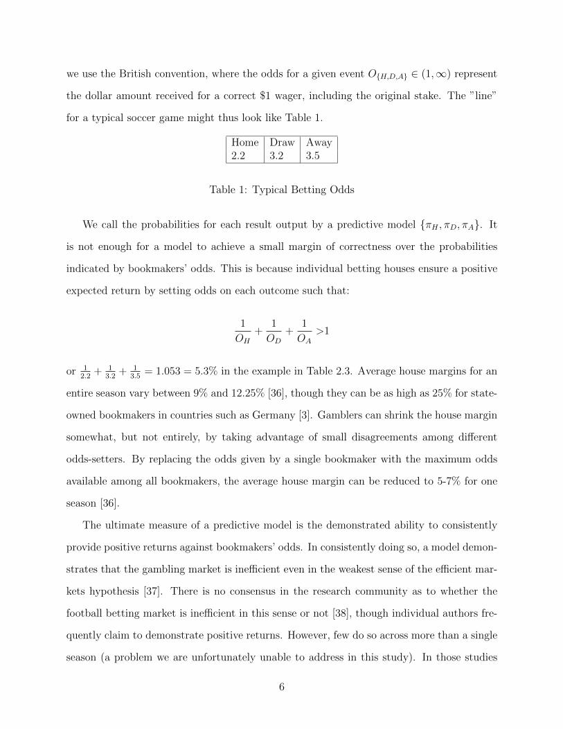
for a typical soccer game might thus look like Table 1.

Home Draw Away2.2 3.2 3.5

Table 1: Typical Betting Odds

We call the probabilities for each result output by a predictive model {πH , πD, πA}. It

is not enough for a model to achieve a small margin of correctness over the probabilities

indicated by bookmakers’ odds. This is because individual betting houses ensure a positive

expected return by setting odds on each outcome such that:

1

OH

+1

OD

+1

OA

>1

or 12.2

+ 13.2

+ 13.5

= 1.053 = 5.3% in the example in Table 2.3. Average house margins for an

entire season vary between 9% and 12.25% [36], though they can be as high as 25% for state-

owned bookmakers in countries such as Germany [3]. Gamblers can shrink the house margin

somewhat, but not entirely, by taking advantage of small disagreements among different

odds-setters. By replacing the odds given by a single bookmaker with the maximum odds

available among all bookmakers, the average house margin can be reduced to 5-7% for one

season [36].

The ultimate measure of a predictive model is the demonstrated ability to consistently

provide positive returns against bookmakers’ odds. In consistently doing so, a model demon-

strates that the gambling market is inefficient even in the weakest sense of the efficient mar-

kets hypothesis [37]. There is no consensus in the research community as to whether the

football betting market is inefficient in this sense or not [38], though individual authors fre-

quently claim to demonstrate positive returns. However, few do so across more than a single

season (a problem we are unfortunately unable to address in this study). In those studies

6

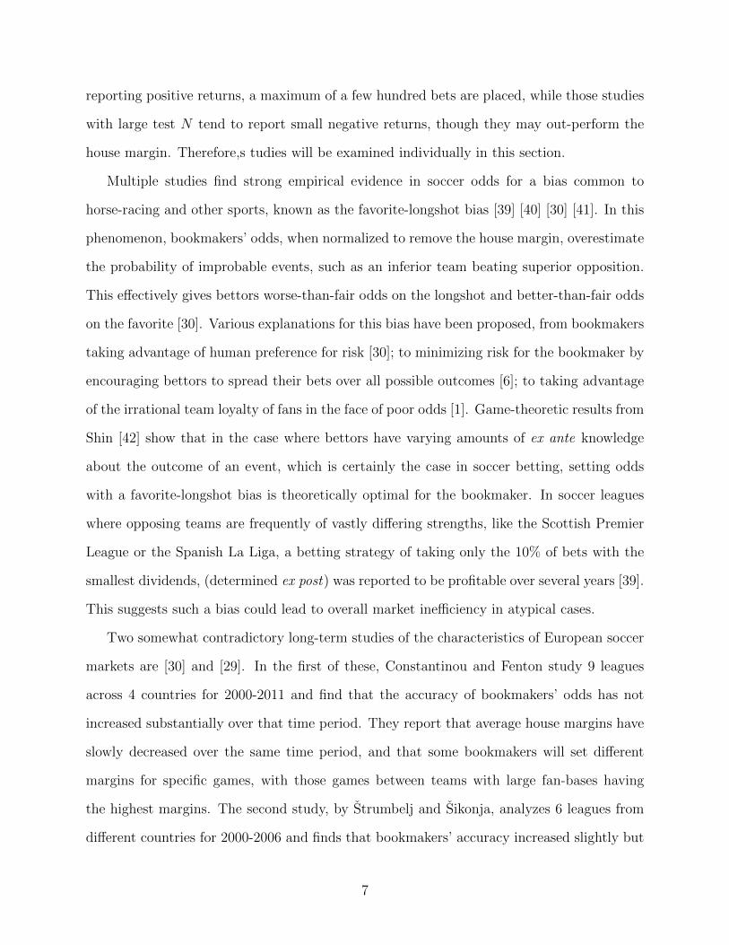
reporting positive returns, a maximum of a few hundred bets are placed, while those studies

with large test N tend to report small negative returns, though they may out-perform the

house margin. Therefore,s tudies will be examined individually in this section.

Multiple studies find strong empirical evidence in soccer odds for a bias common to

horse-racing and other sports, known as the favorite-longshot bias [39] [40] [30] [41]. In this

phenomenon, bookmakers’ odds, when normalized to remove the house margin, overestimate

the probability of improbable events, such as an inferior team beating superior opposition.

This effectively gives bettors worse-than-fair odds on the longshot and better-than-fair odds

on the favorite [30]. Various explanations for this bias have been proposed, from bookmakers

taking advantage of human preference for risk [30]; to minimizing risk for the bookmaker by

encouraging bettors to spread their bets over all possible outcomes [6]; to taking advantage

of the irrational team loyalty of fans in the face of poor odds [1]. Game-theoretic results from

Shin [42] show that in the case where bettors have varying amounts of ex ante knowledge

about the outcome of an event, which is certainly the case in soccer betting, setting odds

with a favorite-longshot bias is theoretically optimal for the bookmaker. In soccer leagues

where opposing teams are frequently of vastly differing strengths, like the Scottish Premier

League or the Spanish La Liga, a betting strategy of taking only the 10% of bets with the

smallest dividends, (determined ex post) was reported to be profitable over several years [39].

This suggests such a bias could lead to overall market inefficiency in atypical cases.

Two somewhat contradictory long-term studies of the characteristics of European soccer

markets are [30] and [29]. In the first of these, Constantinou and Fenton study 9 leagues

across 4 countries for 2000-2011 and find that the accuracy of bookmakers’ odds has not

increased substantially over that time period. They report that average house margins have

slowly decreased over the same time period, and that some bookmakers will set different

margins for specific games, with those games between teams with large fan-bases having

the highest margins. The second study, by Strumbelj and Sikonja, analyzes 6 leagues from

different countries for 2000-2006 and finds that bookmakers’ accuracy increased slightly but

7

significantly over that time period. Strumbelj and Sikonja also contradict Constantinou

and Fenton’s results on house margins for popular teams, finding that those games have

lower margins on average. They conclude that this is due to increased competition among

bookmakers for high betting-volume games. Both studies cite the variability of bookmakers’

accuracy across leagues, as does Marttinen [6], and all conclude that accuracy varies signif-

icantly. While no study of the causes of this variability has been conducted, the authors of

these studies propose that leagues with low betting volume could receive less attention from

the bookmakers, resulting in less accurate odds; and that uneven team strength in certain

leagues, along with the favorite-longshot bias, could reduce apparent accuracy.

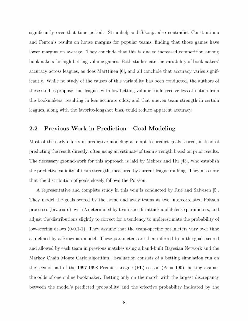
2.2 Previous Work in Prediction - Goal Modeling

Most of the early efforts in predictive modeling attempt to predict goals scored, instead of

predicting the result directly, often using an estimate of team strength based on prior results.

The necessary ground-work for this approach is laid by Mehrez and Hu [43], who establish

the predictive validity of team strength, measured by current league ranking. They also note

that the distribution of goals closely follows the Poisson.

A representative and complete study in this vein is conducted by Rue and Salvesen [5].

They model the goals scored by the home and away teams as two intercorrelated Poisson

processes (bivariate), with λ determined by team-specific attack and defense parameters, and

adjust the distributions slightly to correct for a tendency to underestimate the probability of

low-scoring draws (0-0,1-1). They assume that the team-specific parameters vary over time

as defined by a Brownian model. These parameters are then inferred from the goals scored

and allowed by each team in previous matches using a hand-built Bayesian Network and the

Markov Chain Monte Carlo algorithm. Evaluation consists of a betting simulation run on

the second half of the 1997-1998 Premier League (PL) season (N = 190), betting against

the odds of one online bookmaker. Betting only on the match with the largest discrepancy

between the model’s predicted probability and the effective probability indicated by the

8

bookmaker unadjusted for house margin (∆i = πi − 1/Oi, where i is a result ∈ {H,D,A})

each week gives a 39.6% profit over B = 48 bets, with 15 (31.3%) correct. Running the same

situation on a lower division, they achieve 54.0% profit, B = 64, with 27 (42.2%) correct.

Rue and Salvesen use a betting strategy known as Kelly betting, which varies the fraction

of bankroll bet based on the discrepancy between predicted and offered odds. Kelly betting

will be discussed at length in section 3. They also perform a brief retrospective analysis,

giving examples of teams that performed better or worse than expected over the course of

the season and highlighting the scores of particular matches that deviated strongly from the

model.

A very similar approach that does not model the motion of team strength but does include

the input of betting odds is used by Marttinen [6]. The parameters are fit with a linear

regression instead of an iterated Bayesian approach. Marttinen compares fixed and Kelly

betting with the lower-variance 1/2 Kelly and 1/4 Kelly strategies for one season in seven

different leagues and demonstrates an average profitability of 148.7%, average B = 10.3,

though median profitability was -41.3%, B = 6. Kelly returns far better results in the best

case than either fractional Kelly method, but has significantly higher variance, as expected.

The low number of bets and high variance raise questions of external validity, though the

results strongly suggest that limiting bets to those with expected return (defined for result

i ∈ {H,D,A} as E[ROIi] = πiOi) above a certain threshold can increase performance,

perhaps by compensating for uncertainties in the predictive performance of the model used.

In a comparison between the Bayesian model and one based around Elo rankings, a system

developed for chess, Martinnen finds that the goal-modeling approach performs significantly

better across multiple leagues and seasons.

A slight variation on the Bayesian model of Rue and Salversen is adopted by Baio and

Blangiardo in analyzing the 2007-2008 season of the top Italian soccer league, the Serie A

[44]. They assume that team offensive and defensive strength are drawn from one of three

Gaussian distributions instead of a single distribution, in an attempt to both combat over-

9

fitting and more accurately model a league with teams of very uneven abilities. They do not

perform any quantitative evaluation of their model, but do compare predicted final league

position to actual final league position for each team.

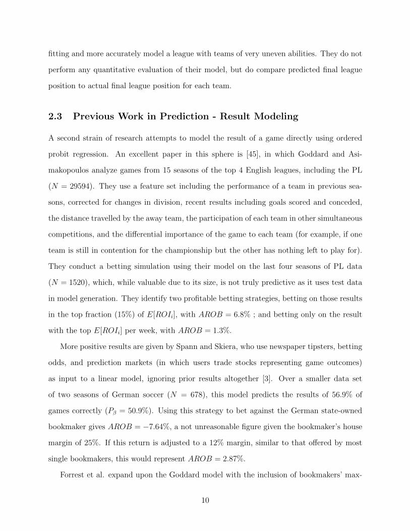
2.3 Previous Work in Prediction - Result Modeling

A second strain of research attempts to model the result of a game directly using ordered

probit regression. An excellent paper in this sphere is [45], in which Goddard and Asi-

makopoulos analyze games from 15 seasons of the top 4 English leagues, including the PL

(N = 29594). They use a feature set including the performance of a team in previous sea-

sons, corrected for changes in division, recent results including goals scored and conceded,

the distance travelled by the away team, the participation of each team in other simultaneous

competitions, and the differential importance of the game to each team (for example, if one

team is still in contention for the championship but the other has nothing left to play for).

They conduct a betting simulation using their model on the last four seasons of PL data

(N = 1520), which, while valuable due to its size, is not truly predictive as it uses test data

in model generation. They identify two profitable betting strategies, betting on those results

in the top fraction (15%) of E[ROIi], with AROB = 6.8% ; and betting only on the result

with the top E[ROIi] per week, with AROB = 1.3%.

More positive results are given by Spann and Skiera, who use newspaper tipsters, betting

odds, and prediction markets (in which users trade stocks representing game outcomes)

as input to a linear model, ignoring prior results altogether [3]. Over a smaller data set

of two seasons of German soccer (N = 678), this model predicts the results of 56.9% of

games correctly (Pβ = 50.9%). Using this strategy to bet against the German state-owned

bookmaker gives AROB = −7.64%, a not unreasonable figure given the bookmaker’s house

margin of 25%. If this return is adjusted to a 12% margin, similar to that offered by most

single bookmakers, this would represent AROB = 2.87%.

Forrest et al. expand upon the Goddard model with the inclusion of bookmakers’ max-

10

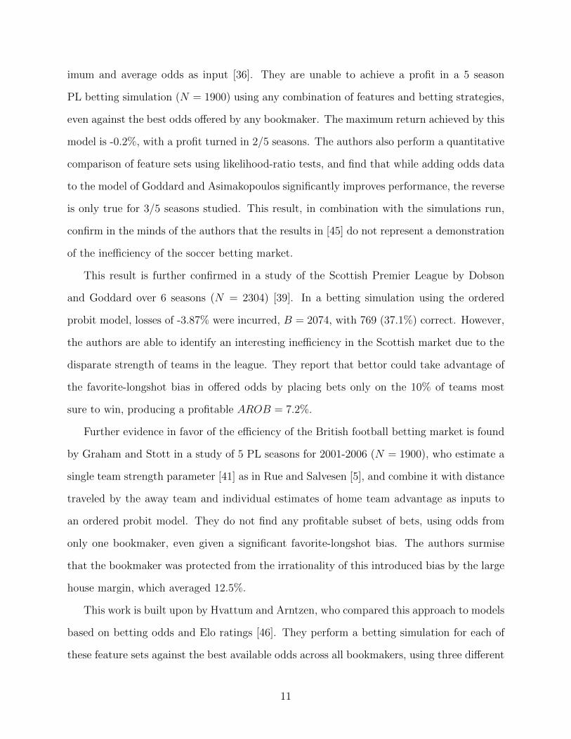
imum and average odds as input [36]. They are unable to achieve a profit in a 5 season

PL betting simulation (N = 1900) using any combination of features and betting strategies,

even against the best odds offered by any bookmaker. The maximum return achieved by this

model is -0.2%, with a profit turned in 2/5 seasons. The authors also perform a quantitative

comparison of feature sets using likelihood-ratio tests, and find that while adding odds data

to the model of Goddard and Asimakopoulos significantly improves performance, the reverse

is only true for 3/5 seasons studied. This result, in combination with the simulations run,

confirm in the minds of the authors that the results in [45] do not represent a demonstration

of the inefficiency of the soccer betting market.

This result is further confirmed in a study of the Scottish Premier League by Dobson

and Goddard over 6 seasons (N = 2304) [39]. In a betting simulation using the ordered

probit model, losses of -3.87% were incurred, B = 2074, with 769 (37.1%) correct. However,

the authors are able to identify an interesting inefficiency in the Scottish market due to the

disparate strength of teams in the league. They report that bettor could take advantage of

the favorite-longshot bias in offered odds by placing bets only on the 10% of teams most

sure to win, producing a profitable AROB = 7.2%.

Further evidence in favor of the efficiency of the British football betting market is found

by Graham and Stott in a study of 5 PL seasons for 2001-2006 (N = 1900), who estimate a

single team strength parameter [41] as in Rue and Salvesen [5], and combine it with distance

traveled by the away team and individual estimates of home team advantage as inputs to

an ordered probit model. They do not find any profitable subset of bets, using odds from

only one bookmaker, even given a significant favorite-longshot bias. The authors surmise

that the bookmaker was protected from the irrationality of this introduced bias by the large

house margin, which averaged 12.5%.

This work is built upon by Hvattum and Arntzen, who compared this approach to models

based on betting odds and Elo ratings [46]. They perform a betting simulation for each of

these feature sets against the best available odds across all bookmakers, using three different

11

betting strategies, for 8 seasons of multiple leagues (N = 15818). This approach is unable

to generate positive returns over any single season in the dataset. The best returns averaged

across the entire test set are given as -4.6% for unit bet, -3.3% for the less risky unit win,

and -5.4% for Kelly, while the maximum odds give an average house margin of 5.5%.

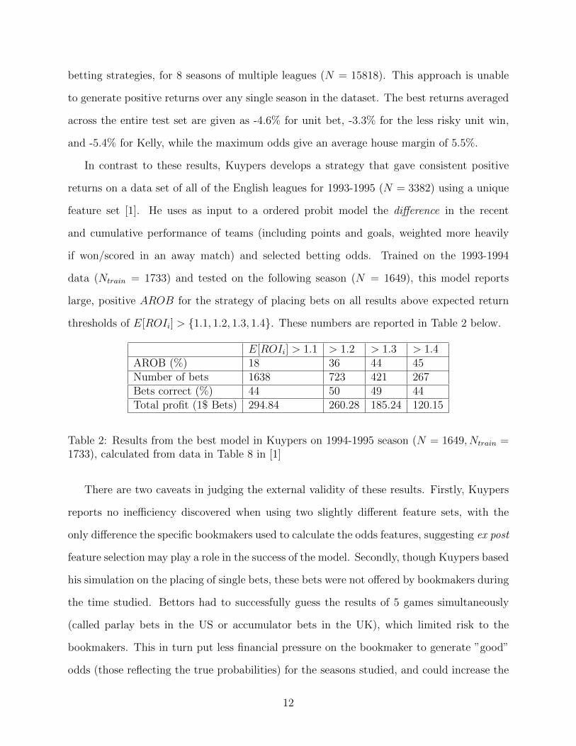
In contrast to these results, Kuypers develops a strategy that gave consistent positive

returns on a data set of all of the English leagues for 1993-1995 (N = 3382) using a unique

feature set [1]. He uses as input to a ordered probit model the difference in the recent

and cumulative performance of teams (including points and goals, weighted more heavily

if won/scored in an away match) and selected betting odds. Trained on the 1993-1994

data (Ntrain = 1733) and tested on the following season (N = 1649), this model reports

large, positive AROB for the strategy of placing bets on all results above expected return

thresholds of E[ROIi] > {1.1, 1.2, 1.3, 1.4}. These numbers are reported in Table 2 below.

E[ROIi] > 1.1 > 1.2 > 1.3 > 1.4AROB (%) 18 36 44 45Number of bets 1638 723 421 267Bets correct (%) 44 50 49 44Total profit (1$ Bets) 294.84 260.28 185.24 120.15

Table 2: Results from the best model in Kuypers on 1994-1995 season (N = 1649, Ntrain =1733), calculated from data in Table 8 in [1]

There are two caveats in judging the external validity of these results. Firstly, Kuypers

reports no inefficiency discovered when using two slightly different feature sets, with the

only difference the specific bookmakers used to calculate the odds features, suggesting ex post

feature selection may play a role in the success of the model. Secondly, though Kuypers based

his simulation on the placing of single bets, these bets were not offered by bookmakers during

the time studied. Bettors had to successfully guess the results of 5 games simultaneously

(called parlay bets in the US or accumulator bets in the UK), which limited risk to the

bookmakers. This in turn put less financial pressure on the bookmaker to generate ”good”

odds (those reflecting the true probabilities) for the seasons studied, and could increase the

12

advantage of a statistically-based approach. Even given these reservations, it is of note that

the number of examples used by Kuypers is larger than any other study reporting positive

results (Rue and Salvesen in [5], Marttinen in [6]), and the bets are profitable for a wider

range of E[ROIi] thresholds than other studies (for example, Goddard [45], or Marttinen).

This suggests that his model does a better job of estimating the true probabilities of each

result.

Positive results possibly indicating market inefficiency are also reported by Constantinou,

et al. [2] on the same set of test data used in this thesis, the 2011-2012 PL season (N = 380).

They use a complex hand-built Bayesian model that incorporates subjective evaluations of

team strength and morale, as well as the results of recent matches, key player presence,

and fatigue. The authors, like Rue and Salversen [5], choose bets to place not based on

E[ROIi] = πiOi, but based on the absolute discrepancy between predicted and indicated

probabilities, ∆i = πi − 1/Oi. As summarized in Constantinou’s previous paper [4], a

betting simulation with this model on the 2010-2011 season (N = 380), using the strategy

of betting on all outcomes with ∆i > 5%, resulted in a profit of 8.40%, B = 169 with 57

(33.7%) correct under a unit betting strategy, with Ntrain = 6244. Full results for this season

can be found in Table 6 of [2]. Constantinou et al.’s results for the same strategy applied to

the 2011-2012 PL season, the same one studied in this thesis, are reported in Table 3. This

model is trained on the 1993-2011 PL seasons (Ntrain = 6624). Their results demonstrate

substantially less profit and far less consistency than those in Kuypers [1], though they are

not directly comparable, as the number of leagues and games tested by Constantinou et al.

is much smaller, and the betting environment has been altered by nearly two decades of

drastic change.

Constantinou et al. compare the strategy of betting on every outcome with ∆i > k ∈

{0%, 1%, . . . , 15%} to one that places bets on only the best outcome per game, and find that

the multiple strategy of betting is superior or equal for all ∆i thresholds, contrary to the

average bettor’s intuition and practice. Constantinou et al. also investigate proportional

13

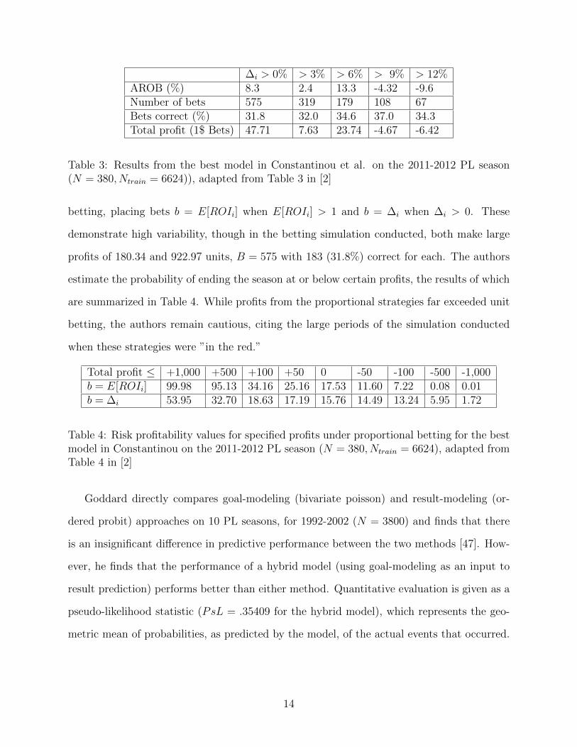
∆i > 0% > 3% > 6% > 9% > 12%AROB (%) 8.3 2.4 13.3 -4.32 -9.6Number of bets 575 319 179 108 67Bets correct (%) 31.8 32.0 34.6 37.0 34.3Total profit (1$ Bets) 47.71 7.63 23.74 -4.67 -6.42

Table 3: Results from the best model in Constantinou et al. on the 2011-2012 PL season(N = 380, Ntrain = 6624)), adapted from Table 3 in [2]

betting, placing bets b = E[ROIi] when E[ROIi] > 1 and b = ∆i when ∆i > 0. These

demonstrate high variability, though in the betting simulation conducted, both make large

profits of 180.34 and 922.97 units, B = 575 with 183 (31.8%) correct for each. The authors

estimate the probability of ending the season at or below certain profits, the results of which

are summarized in Table 4. While profits from the proportional strategies far exceeded unit

betting, the authors remain cautious, citing the large periods of the simulation conducted

when these strategies were ”in the red.”

Total profit ≤ +1,000 +500 +100 +50 0 -50 -100 -500 -1,000b = E[ROIi] 99.98 95.13 34.16 25.16 17.53 11.60 7.22 0.08 0.01b = ∆i 53.95 32.70 18.63 17.19 15.76 14.49 13.24 5.95 1.72

Table 4: Risk profitability values for specified profits under proportional betting for the bestmodel in Constantinou on the 2011-2012 PL season (N = 380, Ntrain = 6624), adapted fromTable 4 in [2]

Goddard directly compares goal-modeling (bivariate poisson) and result-modeling (or-

dered probit) approaches on 10 PL seasons, for 1992-2002 (N = 3800) and finds that there

is an insignificant difference in predictive performance between the two methods [47]. How-

ever, he finds that the performance of a hybrid model (using goal-modeling as an input to

result prediction) performs better than either method. Quantitative evaluation is given as a

pseudo-likelihood statistic (PsL = .35409 for the hybrid model), which represents the geo-

metric mean of probabilities, as predicted by the model, of the actual events that occurred.

14

2.4 Previous Work in Prediction - Neural Networks and Other

Approaches

Various authors also attempt to use common machine learning methods to directly predict

soccer results. Hucaljuk and Rakipovic evaluate an ensemble of methods, including Random

Forests, Artificial Neural Networks, LogitBoost, and k-Nearest Neighbor, on the 2008-2009

European Champions League (N = 96) [48]. Their feature representation includes the results

of previous matches, the goals scored in those matches, the number of players injured on

each team, the result of the previous meeting of the two teams, and the initial seeding of the

teams. They are able to achieve an accuracy of 61.46% (Pβ = 52.1%) using neural networks,

averaged across different training/test splits, though cross validation is not performed.

A neural network-based prediction of the finals stage of the 2006 World Cup (N = 16)

is performed by Huang and Chang [27]. This model uses as input a small subset (m = 8)

of the features used in this thesis but nowhere else in the literature. They aggregate these

statistics for the entire team, whereas we break them down by player. The feature set used

is hand-selected by the authors using their domain knowledge and includes goals scored,

shots, shots on target, corner kicks, direct free kick goals, indirect free kick goals, possession

percentage, and fouls suffered. (Possession percentage was first examined by Hirotsu and

Wright, though they report it has mixed effectiveness as a predictor [49]). The approach of

Huang and Chang correctly predicts the results of 10/16 (62.5%) games (Pβ = 37.5%). The

baseline percentage is much lower in this case, as there are no home or away teams in an

an international tournament held on neutral ground like the World Cup, so the best naive

strategy is to pick a win for a random team. In this type of tournament, any match ending

tied before extra time, and subsequently penalties, is considered a draw by bookmakers,

though all matches are eventually decided for one team or another.

A pair of larger neural network studies examine the second half of the 2001-2002 Italian

Serie A season (N = 154). Cheng et al. [50] use a hierarchical network with a coarse

prediction of the result at the first stage. This first stage takes as input only the average

15

number of points and goals per game. The model’s prediction at the first stage selects one of

three models to be used for the final stage. The final stage receives as input a slightly larger

vector for each team containing a breakdown of previous performance into percent wins,

losses, and draws, average goals for and against, and the results of the most recent 3 games.

This is weighted by a linear penalty parameter favoring the more recent results. This model

predicts 52.3% of games correctly (Pβ = 45.5%), significantly outperforming a model based

on Elo and two simple decision rule heuristics. Aslan and Inceoglu [51] use the same dataset

with a substantially simpler approach that tracks two variables for each team over the course

of the season representing performance at home and away. These are incremented on a win

and decremented on a loss. A neural network with only two inputs, the home performance

of the home team and the away performance of the away team, predicts results with 53.3%

accuracy, slightly edging out Cheng et al.’s result.

An interesting model is proposed by Byungho Min et al. [52], in which the authors sim-

ulate the tactical evolution of a game over time using a combination of rule-based reasoners

and Bayesian networks. Their model incorporates expert evaluations of team strength and

tactical tendencies and is tested on data from the 2002 World Cup (N = 64), though no

quantitative evaluation is reported. Their model more closely simulates the process of a

soccer game than any other published work in the predictive sphere. This type of analysis

certainly merits further investigation and quantitative analysis on a larger scale. It should be

noted that predictive analysis performed ex post that incorporates subjective evaluations of

quality must be treated with special care, as the complete performances of individual teams

and players are known to the expert at the time he or she labels the data.

3 Methods and Data

3.1 Data Used and Parsing Considerations

The data used in the modeling process can be broken down into three principal categories.

16

• Frequency counts of in game events from the 2011-2012 PL season, such as tackles,

shots, yellow cards, and more, recorded for each player individually.

• Betting odds offered by various bookmakers.

• Statistics describing the whole team, including overall performance in previous seasons.

The data of the first type, event frequency counts, were supplied by MCFC and Opta as

part of the Manchester City Analytics program [14]. This data are formatted as a .csv file,

where a line describes a player’s performance in a specific game. All-in-all, counts for 196

different events are included, ranging from frequent, important events, such as tackles, to

infrequent events, such as dribbles. Game events such as minutes played and substitutions on

and off are given, as well as some subjective events, including ”Big Chances,” ”Key Passes,”

etc. Most events are given as total counts and subdivided into multiple categories, such as

aerial duels and ground duels, or in an extreme example, shots on target taken with the

right foot from outside the penalty area. Events with some notion of success, like passes

and duels, are split into unsuccessful and successful counts. We wrote code in Python [53]

to parse this data and aggregate these individual performances into dictionaries of player,

team and game objects, so that this data could be easily used during the process of creating

feature vectors.

Game objects are indexed by a string describing the date (in YYYY-MM-DD for sorting

purposes) and the two teams participating, and contain the performances of each player in

the game indexed by position, links to the object of each player who played in the game,

links to the object of each team, the formation played by each team, and a vector of odds

data. Team objects are indexed by a unique ID assigned by Opta, and contain the schedule

of games played, as well as a vector describing team statistics (see below). Player objects

are also indexed by a unique ID assigned by Opta, and contain the complete performance

history for each player, indexed by game.

17

The betting odds used were collected by the website Football-Data and were downloaded

from [16]. These include fixed odds for every game from the largest 13 international book-

makers. Other types of odds are also included: Asian Handicap Odds from 3 bookmakers,

where one places a bet on one team or the other, with returns defined by a fractional handi-

cap; and over/under odds on 2.5 total goals from 2 bookmakers. Maximum and Average odds

for each of these three bet types are also given, as well as the number of bookmakers used

in their calculation, sourced by Football-Data from the odds aggregator website BetBrain.

These odds were collected on Fridays and Tuesdays, and so may not be collected the same

length of time before each match, as matches can happen on any day of the week. As ”fixed”

odds can change as the bookmaker evaluates additional information [30], it would be more

useful for predictive purposes to have the opening and closing odds for each bookmaker, but

no complete archive of this data for the season used could be found. These data are parsed

in Python, non-odds data is thrown out, and a vector of odds is associated with each game

object.

In order to more completely describe of each team participating in the season studied,

we aggregated information as known at the start of the season from various Internet sources.

The variables and their sources are listed below. (A transfer fee is the fee paid by a club

to negotiate a contract with a player currently employed by another club; trades of players

for players are not as common in professional soccer as they are in American professional

sports.)

• The capacity of the team’s stadium, from the Premier League Handbook [54].

• The location in latitude and longitude of the team’s stadium, collected from Google

Maps, using the addresses provided in [54].

• Statistics describing the team’s performance in the previous season, including rank,

wins, draws, losses, goals for and against, goal difference, and points, also from [54].

• The total amount paid in player wages in the previous season, the rank of this quantity

18

among all teams participating, and the ratio of wages to turnover (profit) for the

financial year ending May 2011, as presented by the Manchester Guardian [55].

• The total cost in transfer fees of the team’s squad as of September 2011, adjusted

for both monetary inflation and inflation in the average transfer fee of PL players, as

calculated by the staff at the Transfer Price Index blog [56].

• The number of matches coached by the team’s manager in the PL, and a historical

residual of that manager’s performance against a regression on squad price, called

m£XIR, also presented on the TPI blog [57].

These data were also parsed in Python and associated with each team object. Three of the

teams did not participate in the Premier League in the previous year, having been promoted

from a lower league. Their performances were approximated by the performances of the three

teams they replaced, using the relative rankings of those teams in the previous year (the

data of the highest ranked newly promoted team replaced by the data of the highest ranked

relegated team). A more desirable alternative approach, given the historical performance

of promoted teams from many seasons, would be to approximate each value using their

lower-league performance and a linear model, but historical data were not available to do

so. Wages and measures of the financial value of a team are included as it is assumed that

they are a good proxy for team skill, given that the market for players has been determined

to be very efficient [13] [8]. A high wages to turnover ratio can indicate a club in financial

trouble, which is popularly believed to affect squad morale and performance. It also gives an

estimate of the financial ability of the club to acquire more players during the season studied,

with lower values giving more freedom to enlist new players. Were more detailed information

available on individual players’ wages and transfer fees, they would be associated with each

player, but team-level information provides an approximate substitute. The m£XIR statistic

is included as a proxy for coaching skill. In the case where a manager has coached < 20 games

in the PL, the m£XIR is given as 0, as these cases were not calculated by the developers

19

of the statistic [57]. A team’s manager might change due to poor performance during the

course of a season, so some teams have data for multiple managers, along with the date(s)

of changeover.

3.2 Feature Representations

As mentioned previously, the principal problem considered in this thesis is the prediction

of the outcome of a soccer game. An instance is a game gi = {yi, xi} ∈ G, outcome

yi ∈ {H,D,A}, and a vector of m features, xi, sourced or calculated from the data presented

above. At every step in the process of transforming raw data into feature representations, care

was taken not to include in xi any information about gi or subsequent games so as to maintain

the validity of the models fitted to G as predictive tools. Many different representations for

xi were considered, all a combination of the subsets of features listed below.

• Team: the team data for the home and away teams as described above, with latitude

and longitude replaced by the distance between the two teams’ stadiums.

• Odds: the odds data for the match, unchanged from the form given above.

• Form-k: the results of the previous k matches for the home and away teams, including

counts of wins, draws, and losses, goals for and against, and shots for and against,

calculated from aggregated frequency count data.

• AllForm: the same counts as Form-k, but averaged over all previous games played

by each team.

• Stats: A set of frequency count-derived statistics, containing only data from one of

the these three sets of games:

1. Prev-k: the previous k games played by each team.

2. Player-k: the previous k games played by each player.

20

3. AllPrev: all previous games, given as average counts per game.

and containing one of these three sets of features for each team:

1. Opta: the entire set of counts for the player playing at each position, ignoring

substitutes (m = 11× 196 = 2156 per team).

2. Jeff: a hand-selected set of counts, containing only those events occurring at

least as frequently as a few times per game, for the player playing at each position

(m = 11× 35 = 385 per team).

3. Key: a set of statistics that are simple functions of the given counts, published by

Opta [58] as Opta Key Stats for use in retrospective player evaluation. These are

different for each position group (Attack, Midfield, Defense, Goalkeeper) and are

calculated for groups as a whole, not for individual players (m = 31 per team).

Distance between teams was calculated from each team’s latitude and longitude using the

Great Circle Distance formula, using code adapted from the first assignment for Princeton’s

COS 126: General Computer Science. This distance was found to be strongly correlated

with the strength of the home team’s advantage by Goddard in studies of the PL [45] [47],

though not in other leagues [39]. All of the team data remain unchanged for each game in

the dataset. Examples of counts included in the Jeff set are interceptions, duels won, and

total unsuccessful passes. Example excluded counts are red cards, headed shots on target

taken from inside the 6 yard box, and off target shots from indirect free kicks. Examples of

statistics in the Key group include saves per goal conceded (Goalkeeper), challenges lost per

minute (Defense), through balls per minute (Midfield) and shots off target per shot on target

(Attack). As each group may have different numbers of players in different formations, all

statistics in the the Key set for each group are divided by the number of players in the

group. A function was written in Python to map position numbers and Opta formation

codes to groups. Once a feature representation is calculated, it is written to disk in a table

format where a row represents a game gi = {yi, xi}, appropriate for use in R or any other

21

statistical analysis language,

3.3 Modeling Approach

In all of the experiments presented in this thesis, a training set of gamesGtest = {g1, . . . , gNtrain}

is used to fit a multinomial logistic regression model with `1 regularization. The glmnet

package [59] was used to generate these models in R [60]. The following brief explanation is

adapted from the associated paper by Friedman et al. [61]. A linear `1-regularized model,

where the response Y is ∈ R, is defined by E(Y |X = x) = β0 + xTβ. In statistical terms,

β0 is called the intercept and β is a vector of the coefficients. Given a set of N examples

(yi, xi), with all variables normalized to 0 mean and unit variance, this model is found by

solving the least-squares problem

min(β0,β)∈Rm+1

[1

2N

N∑i=1

(yi − β0 − xTi β)2 + λm∑j=1

|βj|

](1)

The `1-regularization maximizes the sparsity of the resulting model, and is widely used with

large datasets [61]. Extending this concept to a 3-level multinomial response variable y, as

in our prediction problem, can be done with a logistic model with 3 intercepts and 3 sets of

coefficients of the form

Pr(Y = r|x) =eβ0r+x

T βr∑k∈{H,D,A} e

β0k+xT βk(2)

The more common approach would here use 2 logits asymmetrically, but Friedman et al.

prefer the symmetric approach above. Given the feature vector for an unlabeled test ex-

ample (xt), this model will output probabilities for each result (πH , πD, πA) = (Pr[yt =

H|xt],Pr[yt = D|xt],Pr[yt = A|xt]). The most probable outcome reported, arg max(πH , πD, πA),

is taken as the class prediction of the model and is called yt. Fitting this model is equivalent

22

to maximizing the penalized log likelihood

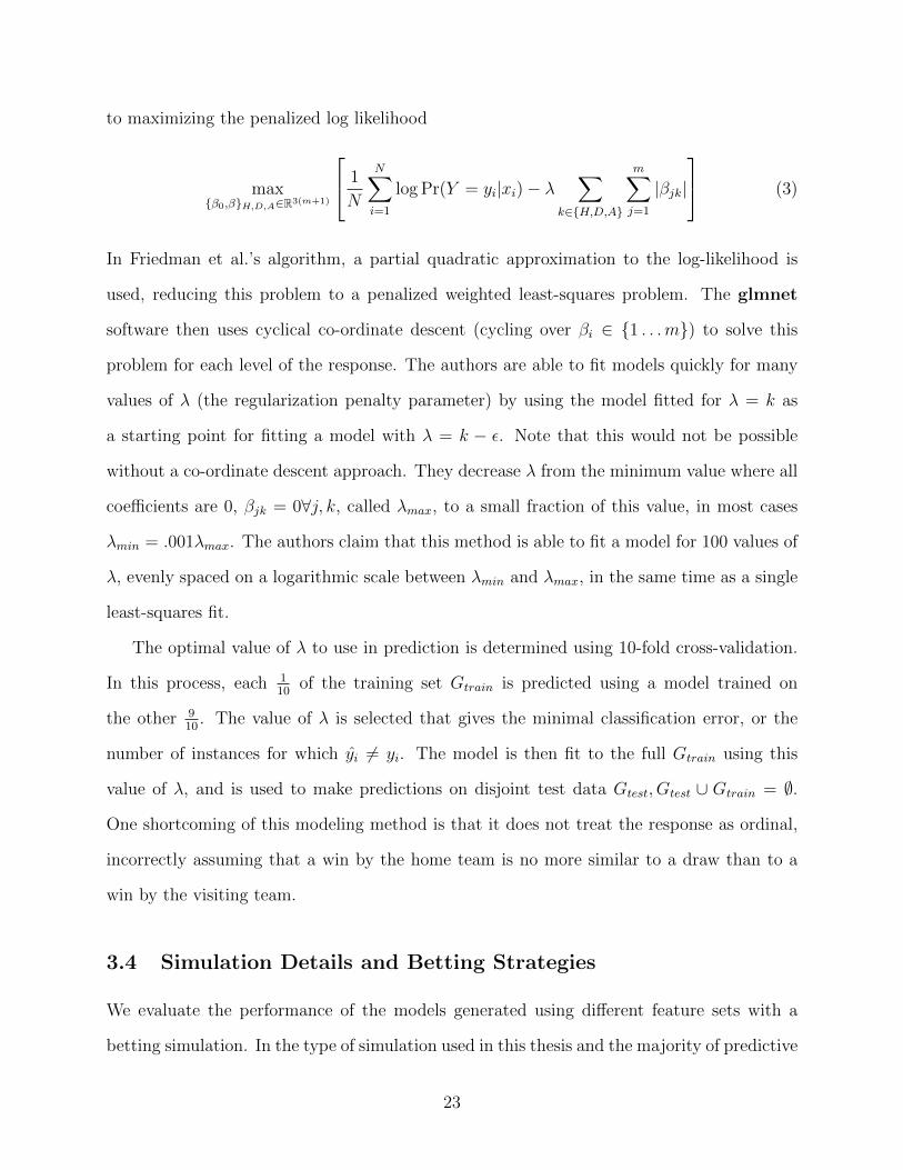
max{β0,β}H,D,A∈R3(m+1)

1

N

N∑i=1

log Pr(Y = yi|xi)− λ∑

k∈{H,D,A}

m∑j=1

|βjk|

(3)

In Friedman et al.’s algorithm, a partial quadratic approximation to the log-likelihood is

used, reducing this problem to a penalized weighted least-squares problem. The glmnet

software then uses cyclical co-ordinate descent (cycling over βi ∈ {1 . . .m}) to solve this

problem for each level of the response. The authors are able to fit models quickly for many

values of λ (the regularization penalty parameter) by using the model fitted for λ = k as

a starting point for fitting a model with λ = k − ε. Note that this would not be possible

without a co-ordinate descent approach. They decrease λ from the minimum value where all

coefficients are 0, βjk = 0∀j, k, called λmax, to a small fraction of this value, in most cases

λmin = .001λmax. The authors claim that this method is able to fit a model for 100 values of

λ, evenly spaced on a logarithmic scale between λmin and λmax, in the same time as a single

least-squares fit.

The optimal value of λ to use in prediction is determined using 10-fold cross-validation.

In this process, each 110

of the training set Gtrain is predicted using a model trained on

the other 910

. The value of λ is selected that gives the minimal classification error, or the

number of instances for which yi 6= yi. The model is then fit to the full Gtrain using this

value of λ, and is used to make predictions on disjoint test data Gtest, Gtest ∪ Gtrain = ∅.

One shortcoming of this modeling method is that it does not treat the response as ordinal,

incorrectly assuming that a win by the home team is no more similar to a draw than to a

win by the visiting team.

3.4 Simulation Details and Betting Strategies

We evaluate the performance of the models generated using different feature sets with a

betting simulation. In the type of simulation used in this thesis and the majority of predictive

23

literature, each game is predicted using a model trained on all previously occurring games.

We decided to treat all games occurring on the same day as simultaneous from the point of

view of the simulation, though games scheduled for the same day may not always overlap.

We decided there was little value in attempting to identify those cases in order to slightly

expand the training set for games starting later in the day, especially given that the frequency

count data used in this thesis is often not released for a full day after each match, due to

extensive verification [14]. In the season studied, games occurred on 100 separate days. We

began all simulations with a Gtrain consisting of those games that occurred on the first 9

of these match-days, Gtrain0 = {g1, . . . , gk}, day(gk+1) = 10, Ntrain0 = 49. At each step, we

add those games predicted in the previous step to Gtrain, refit the model, and predict a new

match-day’s worth of games.

We use the models generated at each step of the simulation to decide not only which

outcomes to bet on, but also how much to bet on each outcome. Returns for each match-day

are added and subtracted to a running total C, which starts with a bankroll of C = 1000

units. Given a fitted model, we decide the amount and size of bets with the help of a betting

strategy. A betting strategy is technically defined as a function that takes three inputs:

• a stake C ≥ 0, the capital remaining after the previous rounds of the simulation

• a vector of odds for each of the 3k possible outcomes of k ≥ 1 games, O ∈ (1,∞)3k

• a vector of predicted probabilities for the same outcomes, π ∈ [0, 1]3k, where the total

probability for the 3 outcomes of every game must sum to 1

A betting strategy outputs a vector of 3k bets b ∈ [0, C], where∑3k

i=1 bi ≤ C, so that the

amount bet does not exceed the available funds.

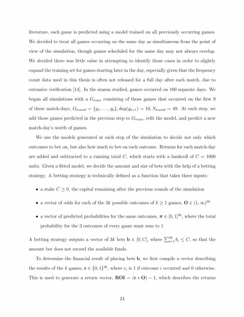
To determine the financial result of placing bets b, we first compile a vector describing

the results of the k games, r ∈ {0, 1}3k, where ri is 1 if outcome i occurred and 0 otherwise.

This is used to generate a return vector, ROI = (r ∗ O) − 1, which describes the returns

24

for a unit bet on each result. Total profit or loss for each round ∆C is equal to the return

vector scaled by the amount bet on each outcome, ∆C = ROI ∗ b.

We compare a total of twelve betting strategies in this thesis. The first three are unit

betting strategies, where bi ∈ {0, 1}. (Remember that E[ROIi] = πiOi and ∆i = πi− 1/Oi.)

1. Naive: We place a unit bet on the outcome predicted by the model for each game,

that with maximum πi.

2. Positive: We place a unit bet on all outcomes for which ∆i > 0

3. Best: For each game, we place a unit bet on the outcome with maximum ∆i, if that

∆i > 0. This is similar to Positive, but places a bet on only one outcome per game.

The remaining betting strategies place proportional bets bi = fiC, f ∈ [0, 1], where the

fraction fi of the stake to bet is determined for each outcome i by a function of O and π.

The proportional strategies used in this thesis are all based around Kelly betting [62], which

places bets to maximize E[logC]. In a repeated favorable game, Kelly betting not only

maximizes the expected value of C after a given number of rounds, but also minimizes the

expected amount of rounds needed to reach a given amount of money Cx. These results are

due to Breiman [63], who describes Kelly betting as conservative, as it bets a fixed fraction

of C given O and π; and diversifying, as it bets on many outcomes, rather than only the

one with the single largest expected return. The Kelly bet for a single outcome i is given by

fiC, where

fi =πiOi − 1

Oi − i=E[ROIi]− 1

Oi − 1(4)

For our purposes, no bet is placed when fi is negative, as this would represent betting

against (or ”shorting”) i. This is not possible in fixed odds soccer betting, but may be

allowed in other betting types, such as prediction markets. The implicit assumption in

applying this formula to gambling is that our predictions π more accurately reflect the true

25

probabilities of each event than the odds set by the bookmaker, even given the house margin.

If this assumption is true, C should grow exponentially for very large N using Kelly Betting.

While Kelly betting is theoretically optimal in many ways, it does expose the bettor to

substantial financial risk [2] [6]. A common strategy to alleviate this risk is to place bets

equal to some fixed fraction of fC, often fC/2 or fC/4 [6]. This strategy, combined with

equation (4), gives us our next three betting strategies.

4. K-Result: We place a bet on outcome i, bi = fiC/3k, if fi > 0 where k is the number

of games (and 3k the number of outcomes) to be bet on.

5. K-Result/2: We bet one half of the amount bet by K-Result, bi = fiC/6k.

6. K-Result/4: We bet one quarter of the amount bet by K-Result, bi = fiC/12k.

Note that we are careful not to violate∑3k

i=1 bi ≤ C. Naively placing bets bi = fiC could

easily result in betting far more money than available, an unwise strategy for any bettor

looking to avoid financial ruin!

While equation (4) maximizes E[logC] for individual results, it does not generalize triv-

ially to multiple interdependent results. In the case of mutually-exclusive results, like those

of a soccer game, it can sometimes maximize expected return to bet on result i where

E[ROIi] ≤ 1, though the above formula will not do so. As an example of this, consider

a game with π = {πH = .6, πD = .4, πA = 0},O = {OH = 4, OD = 2, OA = 2}, giv-

ing π ∗ O = {E[ROIH ] = 2, E[ROID] = .8, E[ROIA] = 0}. Formula (4) would bet only

bH = (1/3)C, which gives E[C] = .6 ∗ 2C + .4 ∗ (2/3)C = 1.47. However, given that

all of the results are mutually exclusive, this E[C] is not actually maximal. For exam-

ple, we can achieve a greater E[C] by betting bH = (1/2)C, bD = (1/2)C, even though

E[ROID] = .8 ≤ 1. This gives E[C] = .6 ∗ 2C + .4 ∗ C = 1.6C.

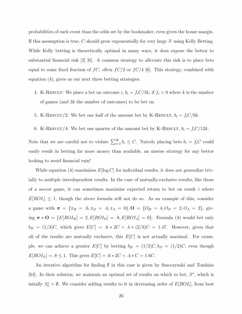
An iterative algorithm for finding f in this case is given by Smoczynski and Tomkins

[64]. In their solution, we maintain an optimal set of results on which to bet, S∗, which is

intially S∗0 = ∅. We consider adding results to it in decreasing order of E[ROIi], from best

26

expected return to worst. In order to decide whether to add a given result i to S∗, we need

to calculate the reserve rate of S∗, notated R(S∗). This is 1 −∑

i∈S∗ fi, or the amount of

the stake that would not be bet in placing Kelly-optimal bets on all outcomes in S∗. R(S∗)

may be calculated by

R(S) =

∑i/∈S∗ πi

1−∑

i∈S∗ 1/Oi

=1−

∑i∈S∗ πi

1−∑

i∈S∗ 1/Oi

(5)

As S∗ is initially empty, R(S∗) is initially = 1. We add a result i to S∗ if (E[ROIi] > R(S∗)

and then recalculate R(S∗). Once the optimal set has been determined, the fraction to

bet for each i ∈ S∗ is given by fi = πi − R(S∗)/Oi. This procedure is fully described in

Algorithm 1.

Algorithm 1 Optimal betting for mutually-exclusive results

INPUT: A vector of odds O = {OH , OD, OA}, and a vector of predicted probabilitiesπ = {πH , πD, πA}

OUTPUT: A vector of fractions f = {fH , fD, fA} of the current stake to bet in order to tomaximize expected returnprocedure M-E Kelly Betting(O,π)

S∗, the optimal set of results to be on, intially ∅R(S∗), the reserve rate of S∗, initially 1E[ROI]← π ∗OE[ROI]← SortDecreasing(E[ROI])for i ∈ E[ROI] do

if E[ROIi] > R(S∗) thenS∗ ← S∗ ∪ iR(S∗)← 1−

∑j∈S∗ πj

1−∑

j∈S∗ 1/Oj

for i ∈ {H,D,A} doif i ∈ S∗ then

fi ← πi − R(S∗)Oi

elsefi ← 0

return f

This algorithm, combined with the risk-alleviating fractional Kelly strategy, gives us our

next three betting strategies. These strategies maximize E[C] for each game.

7. K-Game: For outcome i, we bet bi = fiC/k, where f is generated by Algorithm 1 and

27

k is the number of games to be bet on.

8. K-Game/2: We bet one half of the amount bet by K-Game, bi = fiC/2k.

9. K-Game/4: We bet one quarter of the amount bet by K-Game, bi = fiC/4k.

Again, we are careful not to bet more than we have and violate∑3k

i=1 bi ≤ C.

However, this method can still be further improved. Instead of naively combining the

fi-values generated by Algorithm 1 by assigning a constant fraction of the stake C to each

game, we can bet proportionally more on those outcomes expected to be more profitable.

In order to maximize E[C], in the case where∑3k

i=1 fi ≤ 1, we bet exactly those fractions

suggested by Algorithm 1, bi = fC. When∑3k

i=1 fi > 1 we search for the maximum of

E[C] restricted to the hyperplane∑3k

i=1 fi = 1. A good approximate formula for doing so by

introducing a Lagrange multiplier λ is provided by Maslow and Zhang [65]. In this formula,

f ∗i is the optimal fraction to bet on outcome i, and fi is the fraction returned by Algorithm 1.

f ∗i = (fi − λ)H(fi − λ) (6)

where H(x) is the Heaviside step function, which is 0 for all values < 0 and 1 for all values

≥ 0. The value of λ is found by solving

3k∑i=1

(fi − λ)H(fi − λ) = 1 (7)

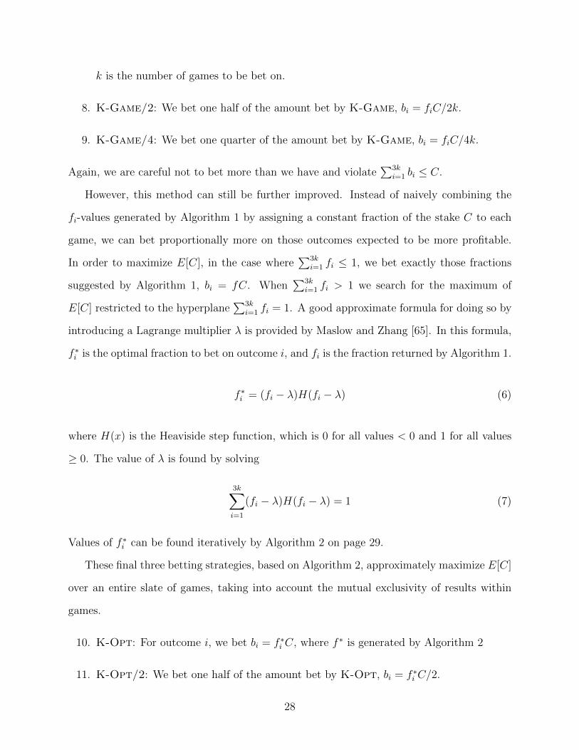
Values of f ∗i can be found iteratively by Algorithm 2 on page 29.

These final three betting strategies, based on Algorithm 2, approximately maximize E[C]

over an entire slate of games, taking into account the mutual exclusivity of results within

games.

10. K-Opt: For outcome i, we bet bi = f ∗i C, where f ∗ is generated by Algorithm 2

11. K-Opt/2: We bet one half of the amount bet by K-Opt, bi = f ∗i C/2.

28

Algorithm 2 Optimal betting on multiple games

INPUT: A vector of 3k fractions f , generated by Algorithm 1OUTPUT: A vector of 3k fractions f∗, such that

∑3ki=1 fi ≤ 1, approximately optimized to

maximize E[C]procedure Optimal Kelly Betting(f∗)

λ, a Lagrange multiplierwhile ||f ||`1 > 1 do

λ← (||f ||`1 − 1)/||f ||`0if fi > λ∀i where fi > 0 then

fi ← fi − λ∀i where fi > 0else

fi ← 0∀i where fi < λ

f∗ ← freturn f∗

12. K-Opt/4: We bet one quarter of the amount bet by K-Opt, bi = f ∗i C/4.

Algorithm 2 is (approximately) optimal in the sense that it maximizes expected return,

given that π represents the true probabilities of the results. However, this definition of

optimality may not be the most appropriate for a real-world bettor. A soccer bettor might

instead prefer to minimize risk, especially given that π represents only the best efforts of

a predictive model, and not true outcome probabilities. Take, for example, the case of an

arbitrage opportunity across bookmakers, where∑

i∈{H,D,A} 1/Oi < 1. The logical bet for a

risk-minimizing gambler is to bet his whole stake such that ∆C > 0 for all possible outcomes,

regardless of the predicted probabilities π. Constantinou et al. found that substituting

arbitrage bets of this form for Kelly bets led to increased profit and reduced risk in betting

simulations of the 2011-2012 PL season [2]. However, we did not attempt to implement

these bets in our simulation, as outside of odds spreadsheets, arbitrage opportunities occur

infrequently and are difficult to exploit [29]. This is because bookmakers identify and remove

these opportunities quickly, often in a matter of seconds for online betting houses [30].

29

4 Results

The results presented in this section derive from a series of simulations conducted as described

in the previous section. The feature sets tested were { Team + Odds + Form-k + {

Player-k, Prev-k } }, k ∈ 1 . . . 7 and { Team + Odds + AllForm + AllPrev

} for each Stats ∈ { Jeff, Key, Opta }. This gives a total of 45 feature sets. We

refer to individual feature sets by a (Games, Stats) pair, i.e. (Prev-2, Key). Results

for each of the 12 betting strategies were collected for models trained on each of these

feature sets. Variables tracked throughout each simulation were the number of bets placed;

the number correct and % correct; and the total profit. Because of the sheer number of

different combinations of feature set and betting strategy, we are sometimes forced to use

representative subsets or aggregate results for analysis.

4.1 General Results and Comparison to Related Work

Across all feature sets and betting strategies, results far exceeding those of all other similar

studies were achieved. Table 5 provides a comparison to the work of all previous authors

who performed unit betting simulations that resulted in a profit. This table does not include

the many studies discussed in section 2 in which no simulations were profitable [36] [39] [41]

[46]. In an effort to provide a single number for comparison among studies of varying N , a

measure of (¢= unit/100) profit per game is included. The two models included in Table 5

from this thesis were not chosen in order to demonstrate the best results that we achieved,

but rather to give an idea of the range of performance of our approach across all feature

sets. These models, (Player-1, Jeff) and (Player-3, Opta) lie at the first and third

quartile Q1, Q3 of final profit. For comparative purposes, the betting strategy used for both

models was Naive. The numbers for Spann are adjusted to approximate 12% house margin,

as given by the authors [3].

Direct comparisons among these results are not always meaningful due to differences

30

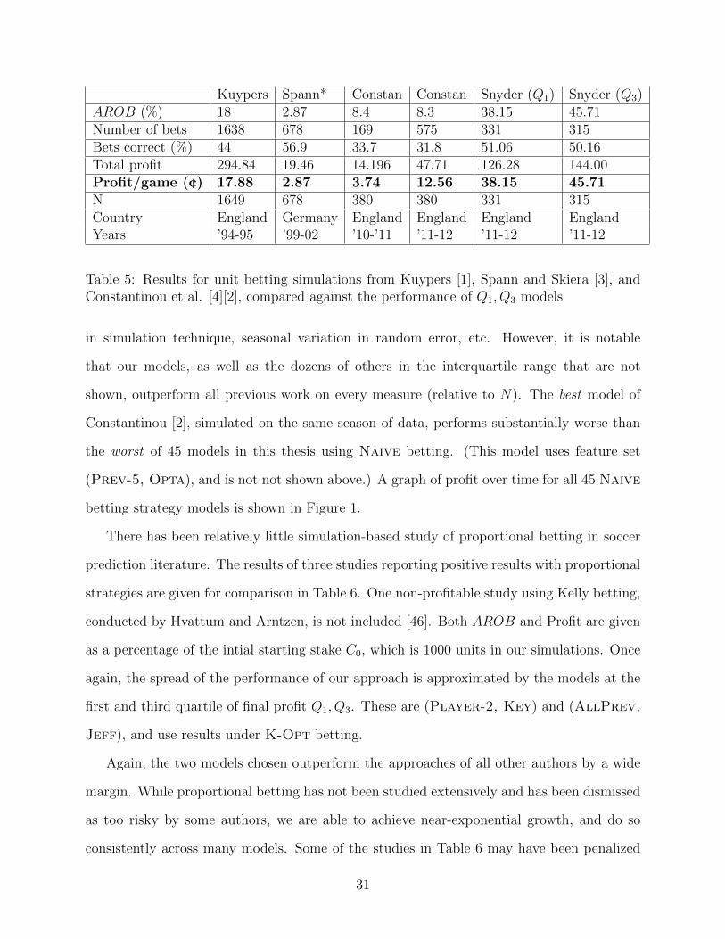
Kuypers Spann* Constan Constan Snyder (Q1) Snyder (Q3)AROB (%) 18 2.87 8.4 8.3 38.15 45.71Number of bets 1638 678 169 575 331 315Bets correct (%) 44 56.9 33.7 31.8 51.06 50.16Total profit 294.84 19.46 14.196 47.71 126.28 144.00Profit/game (¢) 17.88 2.87 3.74 12.56 38.15 45.71N 1649 678 380 380 331 315Country England Germany England England England EnglandYears ’94-95 ’99-02 ’10-’11 ’11-12 ’11-12 ’11-12

Table 5: Results for unit betting simulations from Kuypers [1], Spann and Skiera [3], andConstantinou et al. [4][2], compared against the performance of Q1, Q3 models

in simulation technique, seasonal variation in random error, etc. However, it is notable

that our models, as well as the dozens of others in the interquartile range that are not

shown, outperform all previous work on every measure (relative to N). The best model of

Constantinou [2], simulated on the same season of data, performs substantially worse than

the worst of 45 models in this thesis using Naive betting. (This model uses feature set

(Prev-5, Opta), and is not not shown above.) A graph of profit over time for all 45 Naive

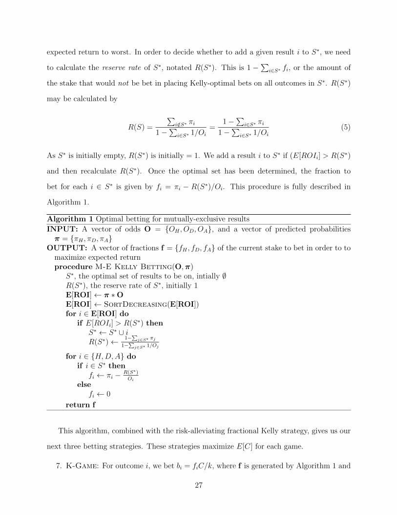
betting strategy models is shown in Figure 1.

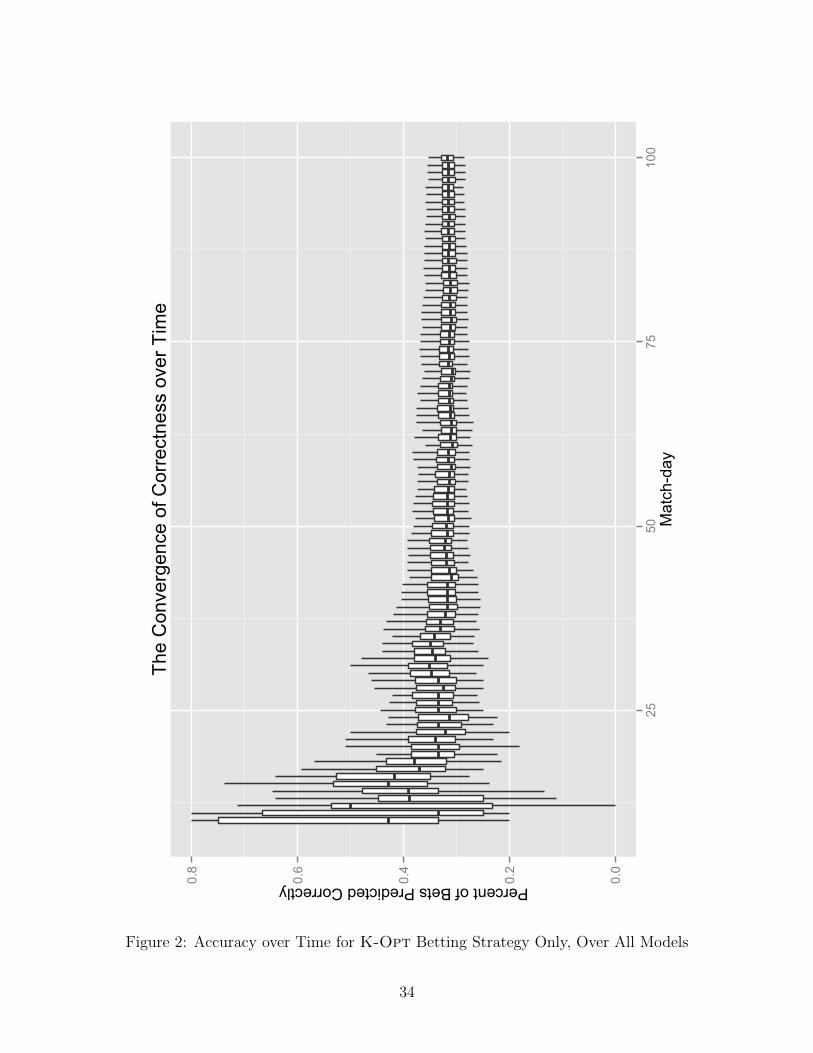
There has been relatively little simulation-based study of proportional betting in soccer

prediction literature. The results of three studies reporting positive results with proportional

strategies are given for comparison in Table 6. One non-profitable study using Kelly betting,

conducted by Hvattum and Arntzen, is not included [46]. Both AROB and Profit are given

as a percentage of the intial starting stake C0, which is 1000 units in our simulations. Once

again, the spread of the performance of our approach is approximated by the models at the

first and third quartile of final profit Q1, Q3. These are (Player-2, Key) and (AllPrev,

Jeff), and use results under K-Opt betting.

Again, the two models chosen outperform the approaches of all other authors by a wide

margin. While proportional betting has not been studied extensively and has been dismissed

as too risky by some authors, we are able to achieve near-exponential growth, and do so

consistently across many models. Some of the studies in Table 6 may have been penalized

31

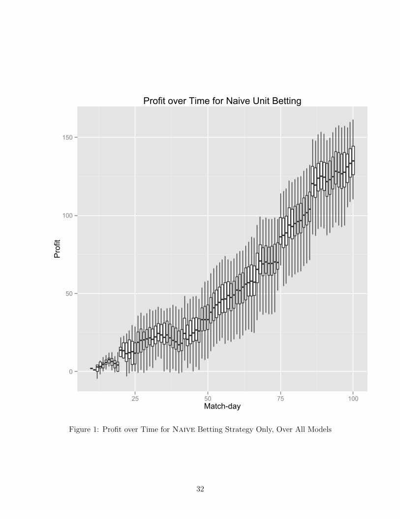
0

50

100

150

25 50 75 100Match-day

Profit

Profit over Time for Naive Unit Betting

Figure 1: Profit over Time for Naive Betting Strategy Only, Over All Models

32

Rue Marttinen Constan Snyder (Q1) Snyder (Q3)AROB (%C0) .83 2.07 .50 .75 4.52Number of bets 48 72 183 452 474Bets correct (%) 31.3 Not Given 31.8 33.4 32.9Profit (%C0) 39.6 148.74 92.30 337.63 1494.94Strategy Kelly Kelly ∆i-based K-Opt K-OptN 190 3028 380 322 331Country England Various England England EnglandYear ’97-98 ’00-01 ’11-12 ’11-12 ’11-12

Table 6: Results for proportional betting simulations from Rue and Salversen [5], Marttinen[6], and Constantinou et al. [2], compared against the performance of Q1, Q3 models

by a sub-optimal implementation of Kelly betting, but the advantage of our model likely

rests in the feature representation used.

Overall, across all 45 ∗ 12 = 540 different combinations of feature set and betting simula-

tion, only 19 cases of negative returns occurred. All of these cases used proportional betting

and 12/19 were one of two feature sets, (Player-4, Opta), and (Player-4, Opta). Across

the set of unit betting strategies, the average profit was 96 units and the median 93 units.

For the set of proportional strategies, the average profit was 2603 units and the median profit

was 954 units. The maximum profit at the end of the simulation was achieved by the feature

vector (Prev-2, Opta), with 66082.92 units, while the maximum % correct was achieved

with (Player-6,Key).

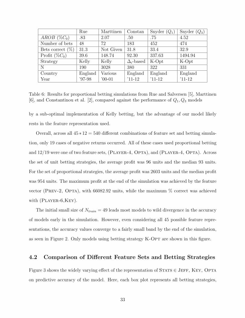
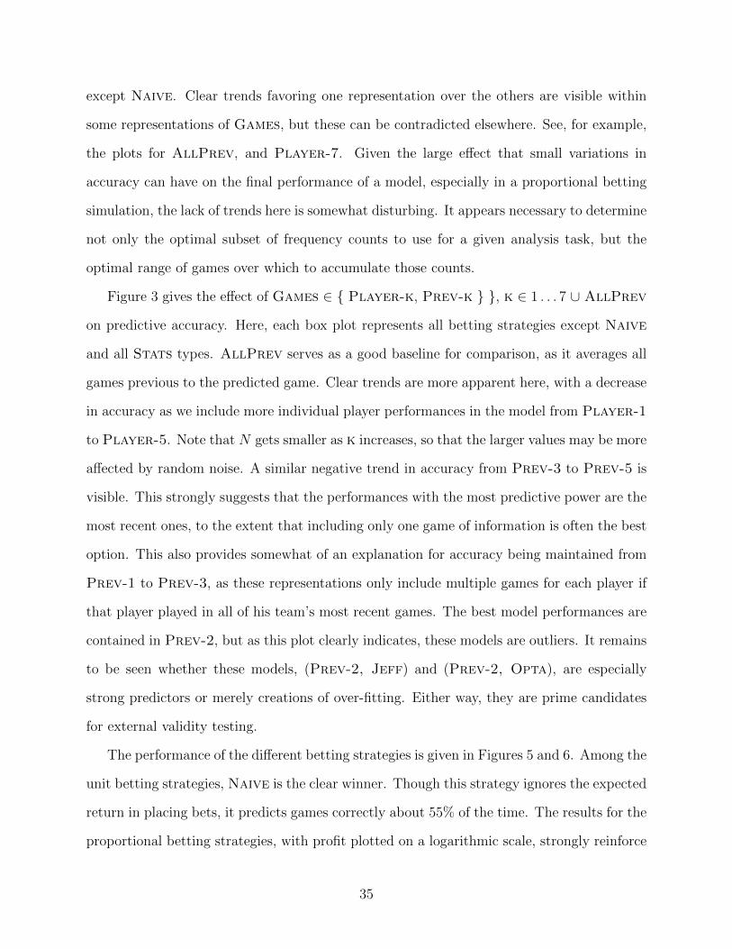
The initial small size of Ntrain = 49 leads most models to wild divergence in the accuracy

of models early in the simulation. However, even considering all 45 possible feature repre-

sentations, the accuracy values converge to a fairly small band by the end of the simulation,

as seen in Figure 2. Only models using betting strategy K-Opt are shown in this figure.

4.2 Comparison of Different Feature Sets and Betting Strategies

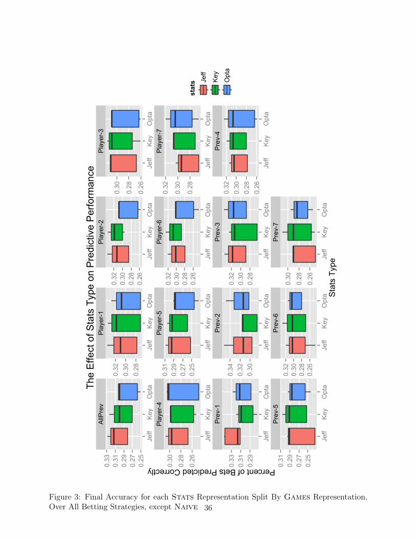
Figure 3 shows the widely varying effect of the representation of Stats ∈ Jeff, Key, Opta

on predictive accuracy of the model. Here, each box plot represents all betting strategies,

33

0.0

0.2

0.4

0.6

0.8

2550

75100

Match-day

Percent of Bets Predicted CorrectlyTh

e C

onve

rgen

ce o

f Cor

rect

ness

ove

r Tim

e

Figure 2: Accuracy over Time for K-Opt Betting Strategy Only, Over All Models

34

except Naive. Clear trends favoring one representation over the others are visible within

some representations of Games, but these can be contradicted elsewhere. See, for example,

the plots for AllPrev, and Player-7. Given the large effect that small variations in

accuracy can have on the final performance of a model, especially in a proportional betting

simulation, the lack of trends here is somewhat disturbing. It appears necessary to determine

not only the optimal subset of frequency counts to use for a given analysis task, but the

optimal range of games over which to accumulate those counts.

Figure 3 gives the effect of Games ∈ { Player-k, Prev-k } }, k ∈ 1 . . . 7 ∪ AllPrev

on predictive accuracy. Here, each box plot represents all betting strategies except Naive

and all Stats types. AllPrev serves as a good baseline for comparison, as it averages all

games previous to the predicted game. Clear trends are more apparent here, with a decrease

in accuracy as we include more individual player performances in the model from Player-1

to Player-5. Note that N gets smaller as k increases, so that the larger values may be more

affected by random noise. A similar negative trend in accuracy from Prev-3 to Prev-5 is

visible. This strongly suggests that the performances with the most predictive power are the

most recent ones, to the extent that including only one game of information is often the best

option. This also provides somewhat of an explanation for accuracy being maintained from

Prev-1 to Prev-3, as these representations only include multiple games for each player if

that player played in all of his team’s most recent games. The best model performances are

contained in Prev-2, but as this plot clearly indicates, these models are outliers. It remains

to be seen whether these models, (Prev-2, Jeff) and (Prev-2, Opta), are especially

strong predictors or merely creations of over-fitting. Either way, they are prime candidates

for external validity testing.

The performance of the different betting strategies is given in Figures 5 and 6. Among the

unit betting strategies, Naive is the clear winner. Though this strategy ignores the expected

return in placing bets, it predicts games correctly about 55% of the time. The results for the

proportional betting strategies, with profit plotted on a logarithmic scale, strongly reinforce

35

AllPrev

Player-1

Player-2

Player-3

Player-4

Player-5

Player-6

Player-7

Prev-1

Prev-2

Prev-3

Prev-4

Prev-5

Prev-6

Prev-7

0.25

0.27

0.29

0.31

0.33

0.28

0.30

0.32

0.26

0.28

0.30

0.32

0.26

0.28

0.30

0.26

0.28

0.30

0.25

0.27

0.29

0.31

0.26

0.28

0.30

0.32

0.28

0.30

0.32

0.29

0.31

0.33

0.30

0.32

0.34

0.28

0.30

0.32

0.26

0.28

0.30

0.32

0.25

0.27

0.29

0.31

0.26

0.28

0.30

0.32

0.26

0.28

0.30

Jeff

Key

Opta

Jeff

Key

Opta

Jeff

Key

Opta

Jeff

Key

Opta

Jeff

Key

Opta

Jeff

Key

Opta

Jeff

Key

Opta

Jeff

Key

Opta

Jeff

Key

Opta

Jeff

Key

Opta

Jeff

Key

Opta

Jeff

Key

Opta

Jeff

Key

Opta

Jeff

Key

Opta

Jeff

Key

Opta

Sta

ts T

ype

Percent of Bets Predicted Correctly

stats Jeff

Key

Opta

The

Effe

ct o

f Sta

ts T

ype

on P

redi

ctiv

e P

erfo

rman

ce

Figure 3: Final Accuracy for each Stats Representation Split By Games Representation,Over All Betting Strategies, except Naive 36

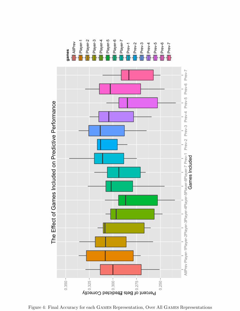
0.250

0.275

0.300

0.325

0.350

AllPrevPlayer-1Player-2Player-3Player-4Player-5Player-6Player-7Prev-1Prev-2Prev-3Prev-4Prev-5Prev-6Prev-7

Gam

es In

clud

ed

Percent of Bets Predicted Correctly

games AllPrev

Player-1

Player-2

Player-3

Player-4

Player-5

Player-6

Player-7

Prev-1

Prev-2

Prev-3

Prev-4

Prev-5

Prev-6

Prev-7

The

Effe

ct o

f Gam

es In

clud

ed o

n P

redi

ctiv

e P

erfo

rman

ce

Figure 4: Final Accuracy for each Games Representation, Over All Games Representationsand Betting Strategies, except Naive

37

not only the superiority of the theoretically optimal model we give in Section 3, but also the

expected ordering K-Result < K-Game < K-Opt. The fractional Kelly strategies do not

appear to minimize risk of loss as effectively as thought, though they do appear to minimize

variability in the financial outcome, to some degree.

5 Conclusion

In this thesis we have used a previously unexplored type of data, the frequency counts

of in-game events, to predict the outcomes of soccer games with more accuracy than any

previous work of similar scope. We extensively reviewed past and current research efforts in

soccer prediction, categorizing their approaches and conclusions. We have also presented an

approximately optimal betting strategy for use in betting simultaneously on multiple games

with mutually-exclusive outcomes, which performs substantially better than other strategies

used in academic betting simulations.

The fact that we were able to achieve such an increase in accuracy with 3 orders of

magnitude more data than used by other authors should not be especially surprising. Indeed,

this thesis has only begun the process of determining the relative importance of these types

of data in prediction and analysis. In the future, more and more complex data will likely

become available faster than we are able to ”solve” problems of feature selection. Moving

forward, it is imperative that predictive and retrospective analyses expand the scope of input

data beyond what is conventional.

We believe that future work in this area has the potential to greatly improve upon the

accuracy of the results presented here, both by incorporating more data and by examining

different modeling approaches. Simple adaptations include capturing the ordinal nature

of the result, and exploring further reductions of the full feature set. Beyond Bayesian

Networks, Neural Networks and simple regression, very few of the large arsenal of modern

machine learning tools have been applied to the problem of soccer prediction. Among the

38

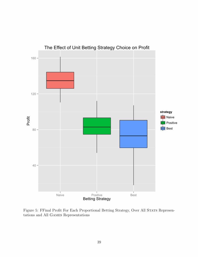
40

80

120

160

Naive Positive BestBetting Strategy

Profit

strategyNaive

Positive

Best

The Effect of Unit Betting Strategy Choice on Profit

Figure 5: FFinal Profit For Each Proportional Betting Strategy, Over All Stats Represen-tations and All Games Representations

39

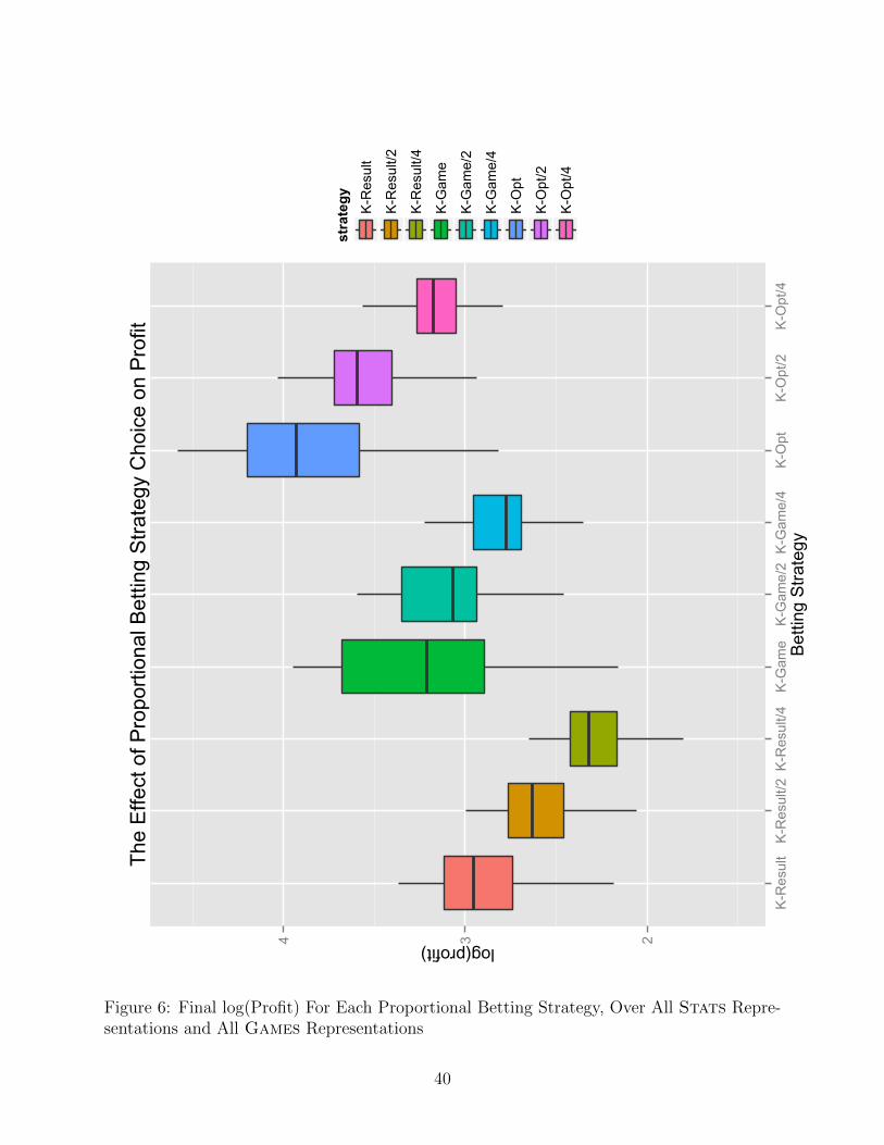
234

K-ResultK-Result/2

K-Result/4

K-Game

K-Game/2K-Game/4

K-Opt

K-Opt/2

K-Opt/4

Bet

ting

Stra

tegy

log(profit)

strategyK-Result

K-Result/2

K-Result/4

K-Game

K-Game/2

K-Game/4

K-Opt

K-Opt/2

K-Opt/4

The

Effe

ct o

f Pro

porti

onal

Bet

ting

Stra

tegy

Cho

ice

on P

rofit

Figure 6: Final log(Profit) For Each Proportional Betting Strategy, Over All Stats Repre-sentations and All Games Representations

40

huge space of possible methods, there are many that may help deal with the frustrating

idiosyncrasies of soccer data. The landscape of explored data is even smaller at present than

that of explored modeling techniques. The next large advance may come from incorporating

crowd-sourced opinion data, network analysis of passing patterns, financial information, or

physical measures.

Most research, including this thesis, treats a match as a result-producing black box,

ignoring the noisy, but beautifully complex processes that contribute to each shot and goal.

As XY data makes its way into the hands of researchers, more detailed models of in-game

processes may be built. This will in turn open up new problems and avenues for analysis,

hopefully leading to a deeper understanding of the game itself.

Looking beyond prediction, there are hundreds of important, valuable questions to be

answered in soccer analytics by the application of statistical techniques, including player

acquisition, lineup selection, optimal training, and many more. Whether for decision-making

or story-telling in the media, analytics has a future in professional soccer. The value of

statistical learning and thinking may not be widely recognized the sport at present, but

there are few better ways to prove the validity of not only a specific model, but also scientific

analysis of sport as a whole, than by making obscene amounts of money in betting.

6 References

[1] Kuypers, T. Applied Economics 2000, 32, 1353–1363.

[2] Constantinou, A. C.; Fenton, N. E.; Neil, M. Under Review. Draft available at:

http://www.constantinou.info/downloads/papers/pimodel12.pdf 2012,

[3] Spann, M.; Skiera, B. Journal of Forecasting 2009, 28, 55–72.

[4] Constantinou, A. C.; Fenton, N. E.; Neil, M. Knowledge-Based Systems 2012,

41

[5] Rue, H.; Salvesen, O. Journal of the Royal Statistical Society: Series D (The Statisti-

cian) 2000, 49, 399–418.

[6] Marttinen, N. Creating a Profitable Betting Strategy for Football by Using Statistical

Modelling ; Citeseer, 2002.

[7] Magowan, A. Can key statistics help prove a player’s value? 2011; http:

//www.bbc.co.uk/blogs/thefootballtacticsblog/2011/11/how_statistics_

shaped_a_hollyw.html.

[8] Dobson, S.; Goddard, J. The economics of football ; Cambridge University Press, 2011.

[9] Wikipedia, WikiProject Football: Fully professional leagues — Wikipedia, The

Free Encyclopedia. 2013; http://en.wikipedia.org/wiki/Wikipedia:WikiProject_

Football/Fully_professional_leagues.

[10] Ltd., F. A. P. L. Premier League Handbook Season 2011/12. 2013; http://www.

premierleague.com/en-gb/about/the-worlds-most-watched-league.html.

[11] Gleave, S. Soccer analytics: treat it like a stop-and-go sport! 2012; http://11tegen11.

net/2012/03/05/soccer-analytics-treat-it-like-a-stop-and-go-sport/.

[12] Lewis, M. Moneyball: The art of winning an unfair game; WW Norton, 2004.

[13] Kuper, S.; Szymanski, S. Why England Lose; HarperSport, 2010.

[14] Fleig, G. Manchester City Analytics Data Release. 2012; http://www.mcfc.co.uk/

mcfcanalytics.

[15] Tenga, A.; Kanstad, D.; Ronglan, L.; Bahr, R. International Journal of Performance

Analysis in Sport 2009, 9, 8–25.

[16] Football-Data, Premier League (FT and HT results, match stats, match, total goals

and AH odds). 2013; http://www.football-data.co.uk/englandm.php.

42

[17] Cotta, C.; Mora, A. M.; Merelo, J. J.; Merelo-Molina, C. Journal of Systems Science

and Complexity 2013, 26, 21–42.

[18] DOrazio, T.; Leo, M. Pattern recognition 2010, 43, 2911–2926.

[19] Gudmundsson, J.; Wolle, T. Football analysis using spatio-temporal tools. 2012.

[20] Grunz, A.; Memmert, D.; Perl, J. Human movement science 2012, 31, 334–343.

[21] Grunz, A.; Memmert, D.; Perl, J. International Journal of Computer Science in Sport

2009, 8, 22–36.

[22] Kim, H.-C.; Kwon, O.; Li, K.-J. Spatial and spatiotemporal analysis of soccer. 2011.

[23] Kang, C.-H.; Hwang, J.-R.; Li, K.-J. Trajectory analysis for soccer players. 2006.

[24] Rampinini, E.; Coutts, A.; Castagna, C.; Sassi, R.; Impellizzeri, F. International Journal

of Sports Medicine 2007, 28, 1018–1024.

[25] Carling, C.; Dupont, G. Journal of sports sciences 2011, 29, 63–71.

[26] Rampinini, E.; Impellizzeri, F. M.; Castagna, C.; Coutts, A. J.; Wisløff, U. Journal of

Science and Medicine in Sport 2009, 12, 227–233.

[27] Huang, K.-Y.; Chang, W.-L. A neural network method for prediction of 2006 World

Cup Football Game. 2010.

[28] Silver, N. A guide to ESPN’s SPI ratings. 2009; http://espn.go.com/soccer/

worldcup/news/_/id/4447078/GuideToSPI.

[29] Strumbelj, E.; Sikonja, M. R. International Journal of Forecasting 2010, 26, 482–488.

[30] Constantinou, A. C.; Fenton, N. E. Under Review, Draft available at:

http://www.constantinou.info/downloads/papers/evidenceOfInefficiency.pdf 2012,

43

[31] Capital, H. G. The Global Internet Gambling Universe: H2 Market Forecasts/Sector Up-

date. 2010; http://www.scribd.com/doc/45677632/h2-Barclays-Pres-20-05-10.

[32] GamblingData, UK Betting Shops: Over-The-Counter Versus Machines. 2012; http:

//www.gamblingdata.com/files/UKBettingShopsNov2012V_1Final.pdf.

[33] Light, G.; Rutledge, K.; Singleton, Q. Thunderbird International Business Review 2011,

53, 747–761.

[34] Drape, J. Needy States Weigh Sport Betting As Leagues Line

Up Against It. 2013; http://www.nytimes.com/2013/03/28/sports/

more-states-look-to-get-in-the-sports-betting-game.html.

[35] Impact, N. G.; (US), P. C. National gambling impact study commission final report ;

The Commission, 1999.

[36] Forrest, D.; Goddard, J.; Simmons, R. International Journal of Forecasting 2005, 21,

551–564.

[37] Malkiel, B. G.; Fama, E. F. The journal of Finance 1970, 25, 383–417.

[38] Stekler, H. O.; Sendor, D.; Verlander, R. International Journal of Forecasting 2010, 26,

606–621.

[39] Dobson, S.; Goddard, J. Statistical Thinking in Sports. Chapman & Hall/CRC Press,

Boca Raton, FL 2008, 91–109.

[40] Cain, M.; Law, D.; Peel, D. Scottish Journal of Political Economy 2000, 47, 25–36.

[41] Graham, I.; Stott, H. Applied Economics 2008, 40, 99–109.

[42] Shin, H. S. The Economic Journal 1991, 101, 1179–1185.

[43] Mehrez, A.; Hu, M. Y. Zeitschrift fur Operations Research 1995, 42, 361–372.

44

[44] Baio, G.; Blangiardo, M. Journal of Applied Statistics 2010, 37, 253–264.

[45] Goddard, J.; Asimakopoulos, I. Modelling football match results and the efficiency of

fixed-odds betting ; 2003.

[46] Hvattum, L. M.; Arntzen, H. International Journal of forecasting 2010, 26, 460–470.

[47] Goddard, J. International Journal of Forecasting 2005, 21, 331–340.

[48] Hucaljuk, J.; Rakipovic, A. Predicting football scores using machine learning techniques.

2011.

[49] Hirotsu, N.; Wright, M. Journal of the Royal Statistical Society: Series D (The Statis-

tician) 2003, 52, 591–602.

[50] Cheng, T.; Cui, D.; Fan, Z.; Zhou, J.; Lu, S. A new model to forecast the results of

matches based on hybrid neural networks in the soccer rating system. 2003.

[51] Aslan, B. G.; Inceoglu, M. M. A comparative study on neural network based soccer

result prediction. 2007.

[52] Min, B.; Kim, J.; Choe, C.; Eom, H.; McKay, R. Knowledge-Based Systems 2008, 21,

551–562.

[53] Van Rossum, G. Python programming language. 1994.

[54] Ltd., F. A. P. L. Premier League Handbook Season 2011/12. 2011; http://www.

premierleague.com/content/dam/premierleague/.

[55] Conn, D. Premier League finances: the full club-by-club breakdown and verdict. 2013.

[56] Devine, D. The 2011/12 TPI Predictions: Post Summer Transfer Window Update. 2011.

[57] Slaton, Z. All-Time Best Managers Versus Transfer Expenditures (an mXIR Analysis).

2012.

45

[58] Lilley, C. Premier League 2011-12: Player Impacts discussion. 2012.

[59] Friedman, J.; Hastie, T.; Tibshirani, R. glmnet: Lasso and elastic-net regularized gen-

eralized linear models. R package version 1.1-3. 2009.

[60] Ihaka, R.; Gentleman, R. Journal of computational and graphical statistics 1996, 5,

299–314.

[61] Friedman, J.; Hastie, T.; Tibshirani, R. Journal of statistical software 2010, 33, 1.

[62] Kelly Jr, J. Information Theory, IRE Transactions on 1956, 2, 185–189.

[63] Breiman, L. Optimal gambling systems for favorable games. 1961.

[64] Smoczynski, P.; Tomkins, D. Mathematical Scientist 2010, 35, 10 – 17.

[65] Maslov, S.; Zhang, Y.-C. International Journal of Theoretical and Applied Finance

1998, 1, 377–387.

46