What are Marine Ecological Time Series telling us about ... · What are Marine Ecological Time Series telling us about the ocean? A status report [ Individual Chapter (PDF) download

IOC-UNESCO TS129

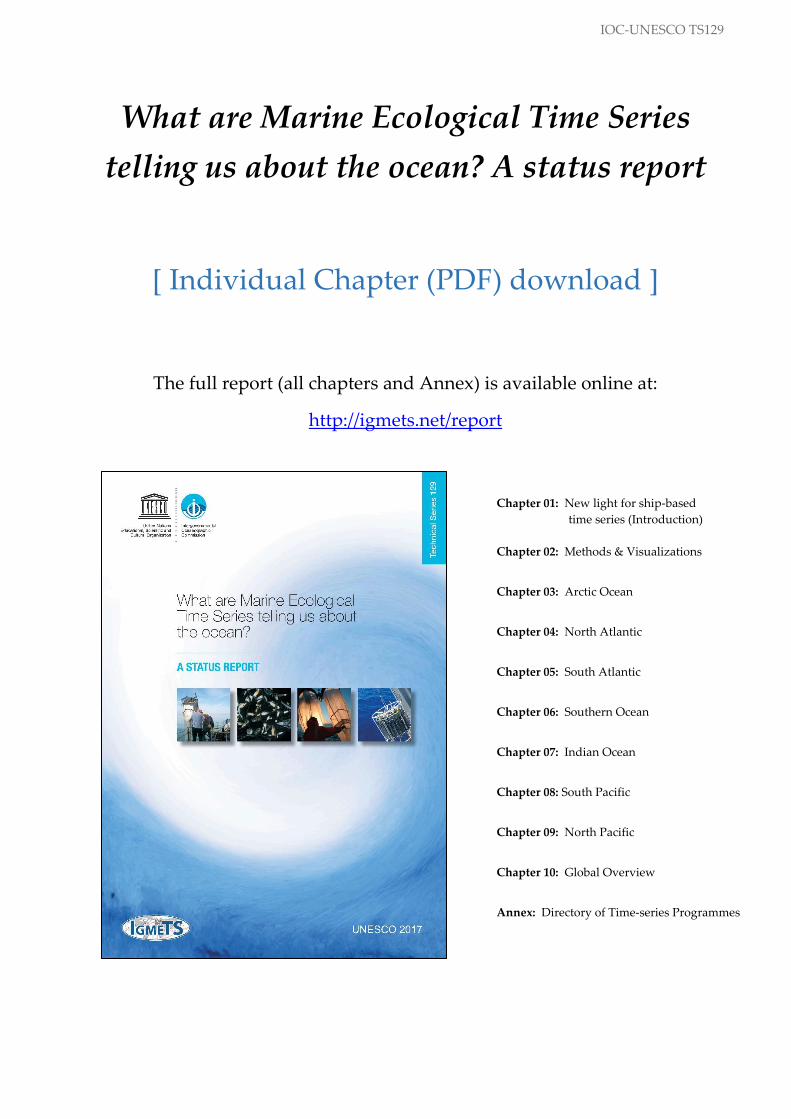
What are Marine Ecological Time Series

telling us about the ocean? A status report

[ Individual Chapter (PDF) download ]

The full report (all chapters and Annex) is available online at:

http://igmets.net/report

Chapter 01: New light for ship-based

time series (Introduction)

Chapter 02: Methods & Visualizations

Chapter 03: Arctic Ocean

Chapter 04: North Atlantic

Chapter 05: South Atlantic

Chapter 06: Southern Ocean

Chapter 07: Indian Ocean

Chapter 08: South Pacific

Chapter 09: North Pacific

Chapter 10: Global Overview

Annex: Directory of Time-series Programmes

http://igmets.net/report

todd.obrien

Rectangle

2

This page intentionally left blank

to preserve pagination in double-sided (booklet) printing

Chapter 10 Global Overview

171

10 Global Overview

Laura Lorenzoni, Todd D. O’Brien, Kirsten Isensee, Heather Benway, Frank E. Muller-

Karger, Peter A. Thompson, Michael Lomas, and Luis Valdés

Figure 10.1. Maps of IGMETS-participating time series on a background of 10-year (2003–2012) sea surface temperature trends (top

panel, see also Figure 10.4a) or on a background of 10-year sea surface chlorophyll trends (bottom panel, see also Figure 10.4b). These

maps show 344 time series (coloured symbols of any type), of which 71 were from Continuous Plankton Recorder subareas (blue box-

es) and 46 were from estuarine areas (yellow stars). Dashed lines indicate boundaries between IGMETS regions. Additional infor-

mation on the sites in this study is presented in the Annex.

172

Participating time-series investigators

Eric Abadie, Jose L. Acuna, M. Teresa Alvarez-Ossorio, Anetta Ameryk, Jeff Anning, Elvire Antajan, Georgia Asima-

kopoulou, Yrene Astor, Angus Atkinson, Patricia Ayon, Alexey Babkov, Hermann Bange, Ana Barbosa, Nick Bates, Uli

Bathmann, Sonia Batten, Beatrice Bec, Radhouan Ben-Hamadou, Claudia Benitez-Nelson, Carla F. Berghoff, Robert Bi-

digare, Antonio Bode, Maarten Boersma, Angel Borja, Alexander Brearley, Eileen Bresnan, Cecilie Broms, Juan Bueno,

Mario O. Carignan, Craig Carlson, David Caron, Jacob Carstensen, Gerardo Casas, Benoit Casault, Claudia Castellani,

Fabienne Cazassus, Georgina Cepeda, Paulo Cesar Abreu, Jacky Chauvin, Sanae Chiba, Luis Chicharo, Epaminondas

Christou, Matthew J. Church, Andrew Clarke, James E. Cloern, Rudi Cloete, Nathalie Cochennec-Laureau, Andrew Cog-

swell, Amandine Collignon, Yves Collos, Frank Coman, Maria Constanza Hozbor, Kathryn Cook, Dolores Cortes, Joana

Cruz, Daniel Cucchi Colleoni, Kim Currie, Padmini Dalpadado, Claire Davies, Alejandro de la Sota, Alessandra de

Olazabal, Laure Devine, Emmanuel Devred, Iole Di Capua, Rita Domingues, Anne Doner, John E. Dore, Antonina dos

Santos, Hugh Ducklow, Janet Duffy-Anderson, Joerg Dutz, Martin Edwards, Lisa Eisner, Joao Pedro Encarnacao, Ruth

Eriksen, Ruben Escribano, Luisa Espinosa, Tone Falkenhaug, Ana Faria, Ed Farley, Maria Luz Fernandez de Puelles, Su-

sana Ferreira, Bjorn Fiedler, Jennifer L. Fisher, James Fishwick, Serena Fonda-Umani, Almudena Fontan, Janja France,

Javier Franco, Jed Fuhrman, Mitsuo Fukuchi, Eilif Gaard, Moira Galbraith, Peter Galbraith, Helena Galvao, Pep Gasol,

Amatzia Genin, Astthor Gislason, Anne Goffart, Renata Goncalves, Rafael Gonzalez-Quiros, Gabriel Gorsky, Annika

Grage, Hafsteinn Gudfinnsson, Kristinn Gudmundsson, Valeria Guinder, Troy Gunderson, David Hanisko, Jon Hare,

Roger Harris, Erica Head, Jean-Henri Hecq, Simeon Hill, Richard Horaeb, Graham Hosie, Jenny Huggett, Keith Hunter,

Anda Ikauniece, Arantza Iriarte, Masao Ishii, Solva Jacobsen, Marie Johansen, Catherine Johnson, Jacqueline Johnson,

Young-Shil Kang, David M. Karl, So Kawaguchi, Kevin Kennington, Diane Kim, Georgs Kornilovs, Arne Kortzinger,

Alexandra Kraberg, Anja Kreiner, Nada Krstulovic, Takahashi Kunio, Inna Kutcheva, Michael Landry, Bertha E. Lavani-

egos, Aitor Laza-Martinez, Jesus Ledesma Rivera, Alain Lefebvre, Sirpa Lehtinen, Maiju Lehtiniemi, Ezequiel Leonarduz-

zi, Ricardo M. Letelier, William Li, Priscilla Licandro, Michael Lomas, Christophe Loots, Angel Lopez-Urrutia, Laura Lo-

renzoni, Roger Lukas, Vivian Lutz, Dave Mackas, Jorge Marcovecchio, Francesca Margiotta, Piotr Margonski, Roberta

Marinelli, Jennifer Martin, Douglas Martinson, Daria Martynova, Daniele Maurer, Maria Grazia Mazzocchi, Sam

McClatchie, Felicity McEnnulty, Webjorn Melle, Jesus M. Mercado, Michael Meredith, Claire Meteigner, Ana Miranda,

Graciela N. Molinari, Nora Montoya, Pedro Morais, Cheryl A. Morgan, Patricija Mozetic, Teja Muha, Frank Muller-

Karger, Jeffrey Napp, Florence Nedelec, Ruben Negri, Vanessa Neves, Todd D. O'Brien, Clarisse Odebrecht, Mark

Ohman, Lena Omli, Emma Orive, Luciano Padovani, Hans Paerl, Marcelo Pajaro, Evgeny Pakhomov, Kevin Pauley, S.A.

Pedersen, Ben Peierls, Pierre Pepin, Myriam Perriere Rumebe, Ian Perry, Tim Perry, William T. Peterson, Roger Petti-

pas, David Pilo, Sophie Pitois, Al Pleudemann, Stephane Plourde, Arno Pollumae, Dwayne Porter, Lutz Postel, Nicole

Poulton, Igor Primakov, Regina Prygunkova, A. Miguel P. Santos, Andy Rees, Michael Reetz, Beatriz Reguera, Malcolm

Reid, Christian Reiss, Jasmin Renz, Mickael Retho, Marta Revilla, Maurizio Ribera, Anthony Richardson, Malcolm

Robb, Marie Robert, Don Robertson, Karen Robinson, M. Carmen Rodriguez, Andrew Ross, Gunta Rubene, M. Guiller-

mina Ruiz, Tatiana Rynearson, Sei-ichi Saitoh, Rafael Salas, Danijela Santic, Diana Sarno, Michael Scarratt, Renate

Scharek, Oscar Schofield, Mary Scranton, Valeria Segura, Sergio Seoane, Stefanija Sestanovic, Yonathan Shaked, Volker

Siegel, Mike Sieracki, Joe Silke, Ricardo I. Silva, Ioanna Siokou-Frangou, Milijan Sisko, Anita Slotwinkski, Tim Smyth,

Mladen Solic, Dominique Soudant, Carla Spetter, Jeff Spry, Michel Starr, Debbie Steinberg, Deborah Steinberg, Lars

Stemmann, Rowena Stern, Solvita Strake, Patrik Stromberg, Glen Tarran, Gordon Taylor, Maria Alexandra Teodosio,

Peter Thompson, Robert Thunell, Valentina Tirelli, Others to be added soon, Mark Tonks, Sakhile Tsotsobe, Ibon Uriarte,

Julian Uribe-Palomino, Nikolay Usov, Luis Valdés, Victoriano Valencia, Marta M. Varela, Hugh Venables, Marina Vera

Diaz, Hans Verheye, Olja Vidjak, Fernando Villate, Maria Delia Viñas, Norbert Wasmund, Robert Weller, George Wiafe,

Claire Widdicombe, Karen H. Wiltshire, Malcolm Woodward, Lidia Yebra, Kedong Yin, Cordula Zenk, Soultana Zervou-

daki, and Adriana Zingone

This chapter should be cited as: Lorenzoni, L., O’Brien, T. D., Isensee, K., Benway, H., Muller-Karger, F. E., Thompson, P. A., Lomas, M., et

al. 2017. Global Overview. In What are Marine Ecological Time Series telling us about the ocean? A status report, pp. 171–190. Ed. by

T. D. O'Brien, L. Lorenzoni, K. Isensee, and L. Valdés. IOC-UNESCO, IOC Technical Series, No. 129. 297 pp.


173

10.1 Introduction

The ocean’s biological, physical, and chemical character-

istics vary across a range of temporal and spatial scales

in response to different driving forces. These include

short-term and seasonal localized phenomena, such as

coastal upwelling and river discharge, as well as meso-

and large-scale features like eddies, ocean currents, and

the global thermohaline circulation – the conveyor belt

(Figure 10.2). The ocean also responds to large-scale cli-

mate cycles (e.g. Pacific Decadal Oscillation, El Niño–

Southern Oscillation, North Atlantic Oscillation).

Changes induced by humans add yet another layer of

complexity. Monitoring changes in global marine biolog-

ical and biogeochemical variables and exploring their

relationships with natural variability and anthropogenic

forcing is fundamental to improving our capacity to

predict how the ocean may respond to future changes as

well as associated impacts on marine ecosystem services

(Worm et al., 2006; Hoegh-Guldberg and Bruno, 2010;

Overland et al., 2010; Doney et al., 2014).

Global ocean phytoplankton biomass and sea surface

temperature (SST) have been investigated with a variety

of techniques, including satellites and in situ sampling.

These two variables have significant effects on ecosys-

tem structure and functioning and have been observed

to change in response to varying ocean conditions

(IPCC, 2013). Several authors have suggested that global

phytoplankton biomass has declined over the past sev-

eral decades in nearly all ocean regions due to increasing

SST and stratification (Behrenfeld et al., 2006; Henson et

al., 2010; Vantrepotte and Mélin, 2009, 2011; Beaulieu et

al., 2013; IPCC, 2013; Siegel et al., 2013), while others

point to an increase in the North Atlantic where long

time series exist (McQuatters-Gollop et al., 2011). The

relationship among SST, chlorophyll and stratification,

however, is not simple; therefore, it is difficult to corre-

late changes in one with changes in the other on a global

scale (Dave and Lozier, 2013; Behrenfeld et al., 2015).

Maps of trends help identify regions that experience

significant changes over different time-scales and can

also provide information on rates of change. Maps of

multiple variables help elucidate possible causes for the

alterations. Changes are constantly occurring on a global

scale; some are related to anthropogenic forcing, and

some variables will show changes faster than others,

resulting in a widespread debate on the length of time

required to observe trends related to climate signals

(Henson et al., 2010, 2016; Henson, 2014).

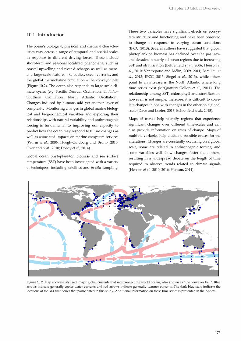
Figure 10.2. Map showing stylized, major global currents that interconnect the world oceans, also known as “the conveyor belt”. Blue

arrows indicate generally cooler water currents and red arrows indicate generally warmer currents. The dark blue stars indicate the

locations of the 344 time series that participated in this study. Additional information on these time series is presented in the Annex.

174

TW05 sites (2008-2012)

TW10 sites (2003-2012)

TW15 sites (1998-2012)

TW20 sites (1993-2012)

TW25 sites (1988-2012)

TW30 sites (1983-2012)

Figure 10.3. Panel of maps showing locations of IGMETS-participating time series based on time-window qualification. Red symbols

indicate time-series sites with at least one biological or biogeochemical variable (i.e. excluding temperature- and salinity-only time

series) that qualified for that time-window (e.g. TW05, TW20). Light gray symbols indicate sites that did not have enough data from

the given time-window to be included in that analysis.

Globally, there are at least 344 ship-based biogeochemi-

cal time series that span different lengths and windows

of time (Figure 10.1). These time series represent one of

the most valuable tools scientists have to characterize

and quantify ocean carbon fluxes, biogeochemical pro-

cesses, and their links to changing climate (Karl, 2010;

Chavez et al., 2011; Church et al., 2013). Coupling these in

situ biogeochemical measurements and plankton data

with satellite observations improves the understanding

of changes in the biological, physical, and biogeochemi-

cal properties of the global oceans. Satellite data provide

an additional layer of information about changing ocean

conditions and ecosystems and can help scale-up the

relatively sparse shipboard datasets to achieve a broader

regional and/or global perspective.

In this chapter, we aim to examine changes in the global

oceans, explore possible connections between ocean ba-

sins, and identify areas that show significant changes

over temporal periods of 10, 15, 20, and 30 years (“time-

windows”; the IGMETS “time-windows” analysis is

described in Chapter 2). A shorter 5-year time-window

analysis is also available to observe short-term fluctua-


175

tions, though these may not be statistically significant

for climate change-related trends. Thirty years of obser-

vations provide information on the overall direction of

change (if any) of the different ocean variables and pre-

sent a good basis to start distinguishing between natural

variability and long-term, human-induced trends (Hen-

son et al., 2010; Henson, 2014). In terms of available bio-

geochemical and plankton time series, there are tenfold

more 5-year time series than 30-year time series. How-

ever, going back in time (20 years), most of the time-

series sites are located in the North Atlantic (Fig-

ure 10.3).

Short time-windows, such as five years, provide infor-

mation on the speed of some of the changes that are be-

ing observed in the ocean and offer insight on short-term

fluctuations. The magnitude of natural variability in

many biogeochemical variables can mask anthropogenic

trends, as is shown in the regional chapters. The ecologi-

cal and economic consequences of such changes are im-

portant, particularly with regard to marine ecosystem

goods and services. Analyzing changes in specific time-

windows facilitates comparison of trends in different

areas and detection of decadal and multidecadal climatic

drivers. Clearly, the start and end dates chosen for trend

analyses may influence the assessment of the rates of

change (IPCC, 2013; Karl et al., 2015).

It is not possible yet to fully quantify how much of the

ocean’s variability is due to anthropogenic drivers;

hence, the importance of sustained ocean time-series

observations. Only a fraction of the biogeochemical time

series around the world reaches or exceeds observations

of more than two decades (Figure 10.3). Indeed, many

ship-based biogeochemical time-series measurements

(e.g. ocean CO2 system parameters, nutrient concentra-

tions), particularly in the southern hemisphere, were

initiated only in the past decade. These various time

series provide a “baseline” against which to detect areas

that have undergone rapid change.

10.2 General patterns of temperature and

phytoplankton biomass

Significant trends in SST were visible at the global scale

(over 79% of the ocean) during the past three decades

(Figure 10.4a; Table 10.1). In the 30-year time-window

(1983–2012), 79.9% (69.8% at p < 0.05) of the world’s

oceans increased in temperature, while 20.1% (13.2% at

p < 0.05) registered a decrease (Table 10.1). The most

significant warming was observed in the Atlantic and

Indian oceans (Figure 10.4a; see also the respective re-

gional chapters). Comparing the changes, the positive

trend was +0.1 to +0.5°C decade–1. Areas that cooled

down had rates of less than –0.1°C decade–1. These ob-

servations generally agree with published results that

highlight increases in ocean temperatures of ca. 0.1°C

decade–1 (IPCC, 2013; Karl et al., 2015). Non-significant

changes were visible only in the western and tropical

Pacific Ocean, a portion of the South Atlantic, and in

small areas of the Arctic and Antarctic oceans. The

warming trend is also visible over a large portion of the

global ocean during the past 10–15 years (49.3% in the

past 10 years, with 26.3% at p < 0.05; 69.3% over the past

15 years, with 44.8% at p < 0.05; Figure 10.4a; Table 10.1).

Satellite data coverage of the Arctic region is poor.

Changes in SST show that this area is subject to strong

interannual and spatial variability linked to changes in

albedo (sea ice cover, soot on snow), atmospheric cloud

cover, water vapor and black carbon content, and ocean-

ic heat flux (see Serreze and Barry, 2011; and references

therein). Compared to the Antarctic (with the exception

of the Western Antarctic Peninsula; Meredith and King,

2005; Steig et al., 2009), warming over the Arctic during

1983–2012 has been pronounced (85.3%, with 79.2% at

p < 0.05). While the Arctic Ocean showed a slowdown in

its warming during 2003–2012, positive SST trends have

prevailed.

In the Southern Ocean, 55.9% (with 44% at p < 0.05) of

the region cooled during 1983–2012 (Figures 10.4a

and 10.5). Areas of cooling are close to the Antarctic

coastline, while the warming is observed farther north.

One exception is the area adjacent to the Western Ant-

arctic Peninsula; this warming arises largely from in-

creased air temperatures recorded in the region and re-

duced sea ice cover (Meredith and King, 2005; Steig et

al., 2009; Ducklow et al., 2013). Variations in the Antarc-

tic SST are associated with changes in the polarity of the

Southern Oscillation (SO) and the Southern Annular

Mode (SAM), as well as the Antarctic Oscillation Index

(AAO) (Yu et al., 2012). Some of the colder SSTs ob-

served could be attributed to lower air temperatures

reported for a large portion of the Antarctic Peninsula

(Kwok and Comiso, 2002; Marshall et al., 2014). The

driver of these negative SST trends is still being debated

(Randel and Wu, 1999; Thompson and Solomon, 2002).

Over the 15-year time-window, significant warming was

observed in most of the measurable surface of the

176

Figure 10.4. Annual trends in global sea surface temperature (SST) (a) and sea surface chlorophyll (CHL) (b) and correlations between

chlorophyll and sea surface temperature for each of the standard IGMETS time-windows (c). See “Methods” chapter for a complete

description and methodology used.


177

Southern Ocean (57.5%, of which 40.0% was significant

at p < 0.05; Table 6.1; Figure 6.2). This pattern reversed

over the past 10 years, where ca. 54% of the Southern

Ocean exhibited cooling (Table 6.1; Figure 6.2). The

Western Antarctic Peninsula was still the exception,

where sustained warming was observed in both time-

windows (Meredith and King, 2005; Ducklow et al., 2013;

see Chapter 6). The cooling in the past decade has been,

in part, attributed to the ozone hole (Marshall et al.,

2014).

In the Atlantic Ocean, the subtropical South Atlantic

cooling observed over the 30-year time-period is possi-

bly linked to variations in the subtropical anticyclone

that arises from decadal-scale, wind-driven ocean tem-

perature fluctuations that occur in a north–south dipole

structure (Venegas et al., 1997). It could also be a mani-

festation of an ENSO teleconnection (Nobre and Shukla,

1996; Enfield and Mestas-Nuñez, 2000; Deser et al., 2010).

The warming of the entire North Atlantic region (99.1%,

with 97.3% at p < 0.05) over the past three decades has

been attributed to both natural and anthropogenic forc-

ings (Knudsen et al., 2011; Hoegh-Guldberg et al., 2014).

Over shorter time-scales, the warming and cooling

across the Atlantic were more heterogeneous; during

2003–2012, 50.3% of the Atlantic – the southern north

and south parts – warmed, while 49.7% – the northern

North and South Atlantic – cooled. In the North Atlantic,

air temperatures are largely driven by the NAO, with

colder conditions over the Mediterranean and subpolar

regions and warmer mid-latitudes (Europe, the north-

eastern United States, and parts of Scandinavia) during

positive NAO phases (Visbeck et al., 2001; Deser et al.,

2010; Hurrell and Deser, 2010). For this phase, SST re-

flects a “tripole pattern” with a cold anomaly in the sub-

polar region, a warm anomaly in the mid-latitudes, and

a cold subtropical anomaly between 0 and 30°N (Visbeck

et al., 2001). The mixed warm/cold trends observed in the

North Atlantic over the past decade could be reflecting

fluctuations of NAO phases (e.g. strong negative phases

in 2009 and 2010, positive in 2012), and possible SST

feedback (Hurrell and Deser, 2010; Figure 10.4). The

colder SST could also be the result of changes in the At-

lantic meridional overturning circulation (AMOC), as

suggested by Rahmstorf et al. (2015).

Cooling observed in the western and tropical Pacific

Ocean over the past 30 years is likely related to interan-

nual–multidecadal oscillations like the El Niño Southern

Oscillation (ENSO), the Interdecadal Pacific Oscillation

(IPO), and the Pacific Decadal Oscillation (PDO)

(Chavez et al., 2003, 2011). Pacific SST is strongly corre-

lated with these climate indices (Enfield et al., 2001; Al-

exander et al., 2002). The warming and cooling of the

Pacific under the changing regimes is not uniform; the

central North and South Pacific are out of phase with the

eastern Pacific. Chavez et al. (2003) identified one

“warm” period (from about 1975 to the late 1990s) and

two cooler periods (from the early 1950s to about 1975

and from the late 1990s to around 2012). In the 15-year

time-window, a particular pattern emerged in the Pacific

Ocean with warming across the equatorial Pacific. In

1998–2012, 65.2% of the Pacific warmed (37% at p < 0.05),

and these areas were located mostly near the equator

and in the central North and South Pacific; 34.8% cooled

(17.0% at p < 0.05; see Figure 7.2). That pattern can be

tied to ENSO (Deser et al., 2010). However, when analyz-

ing the 10-year time-window, the Pacific exhibited a

general cooling over 59% of its area (40% at p < 0.05).

This is largely linked to La Niña-like conditions (Kosaka

and Xie, 2013) and a change in phase of IPO from posi-

tive to negative around 1998/1999 (Dong and Zhou,

2014).

The Indian Ocean exhibited strong, consistent warming

across all time-windows. From 1983 to 2012, 97.8% of the

Indian Ocean warmed (91.9% at p < 0.05; Figure 10.4).

The warming is associated with a range of climate cy-

cles, including the IPO (Han et al., 2014). Over shorter

time-scales (10–15 years), while the sustained warming

prevailed, the spatial extent decreased (Table 10.1), like-

ly due to variability induced by shorter-term climatic

signals (e.g. Indian Ocean Dipole, ENSO).

The chlorophyll (Chl a) trends, as derived from satellite

data, show that, overall, ca. 60% of the ocean has exhib-

ited decreasing concentrations over the past 15 years

(Figures 10.4 and 10.5), which is consistent with previ-

ous studies (Polovina et al., 2008; Henson et al., 2010;

Siegel et al., 2013; Gregg and Rousseaux, 2014; Signorini

et al., 2015). In general, changes in chlorophyll are in-

versely related to SST (Table 10.1; Figure 10.4). The in-

crease in global Chl a concentrations observed in the 10-

year time-window, relative to the 15-year window,

might be attributable to somewhat cooler SSTs. In the

Pacific Ocean, in particular, higher Chl a concentrations

were observed in the subtropics, between roughly 10

and 30°, both north and south of the equator. This region

corresponds to areas experiencing cooling and possibly

becoming more productive (increased mixed-layer

depth), due to La Niña-like conditions (Siegel et al., 2013;

Signorini et al., 2015). The influences of circulation pat

178

Table 10.1. Relative spatial areas (% of the total region) and rates of change that are showing increasing or decreasing trends in sea

surface temperature (SST) for each of the standard IGMETS time-windows. Numbers in brackets indicate the % area with significant

(p < 0.05) trends. See “Methods” chapter for a complete description and methodology used.

Latitude-adjusted SST data field

surface area = 361.9 million km2

5-year (2008–2012)

10-year (2003–2012)

15-year (1998–2012)

20-year (1993–2012)

25-year (1988–2012)

30-year (1983–2012)

Area (%) w/ increasing SST trends

(p < 0.05) 52.9%

( 14.8% )

49.3%

( 26.3% ) 69.3%

( 44.8% ) 74.1%

( 60.8% ) 79.4%

( 67.5% ) 79.9%

( 69.8% )

Area (%) w/ decreasing SST trends

(p < 0.05)

47.1%

( 16.4% ) 50.7%

( 29.7% )

30.7%

( 15.0% )

25.9%

( 15.6% )

20.6%

( 13.0% )

20.1%

( 13.2% )

> 1.0°C decade–1 warming

(p < 0.05)

14.3%

( 9.4% )

4.2%

( 4.2% )

0.6%

( 0.6% )

0.1%

( 0.1% )

0.0%

( 0.0% )

0.0%

( 0.0% )

0.5 to 1.0°C decade–1 warming

(p < 0.05)

14.5%

( 3.8% )

11.3%

( 10.6% )

7.3%

( 7.2% )

6.0%

( 6.0% )

1.9%

( 1.9% )

1.6%

( 1.6% )


(p < 0.05)

17.4%

( 1.3% )

25.0%

( 11.2% )

46.4%

( 35.2% ) 54.9%

( 51.7% ) 59.6%

( 58.5% ) 58.4%

( 58.1% )


(p < 0.05)

6.8%

( 0.3% )

8.8%

( 0.3% )

15.1%

( 1.8% )

13.1%

( 3.0% )

17.8%

( 7.0% )

19.9%

( 10.1% )

0.0 to –0.1°C decade–1 cooling

(p < 0.05)

5.3%

( 0.1% )

9.5%

( 1.4% )

12.6%

( 2.8% )

12.5%

( 4.1% )

12.6%

( 5.4% )

14.0%

( 7.2% )

–0.1 to –0.5°C decade–1 cooling

(p < 0.05)

14.9%

( 0.9% )

24.2%

( 11.9% )

16.3%

( 10.4% )

12.3%

( 10.4% )

8.1%

( 7.6% )

6.1%

( 5.9% )

–0.5 to –1.0°C decade–1 cooling

(p < 0.05)

12.2%

( 4.1% )

13.2%

( 12.6% )

1.6%

( 1.6% )

1.1%

( 1.1% )

0.0%

( 0.0% ) 0.0 %

> –1.0°C decade–1 cooling

(p < 0.05)

14.6%

( 11.2% )

3.9%

( 3.8% )

0.1%

( 0.1% ) 0.0 % 0.0 % 0.0 %

Table 10.2 Relative spatial areas (% of the total region) and rates of change that are showing increasing or decreasing trends in phyto-

plankton biomass (CHL) for each of the standard IGMETS time-windows. Numbers in brackets indicate the % area with significant

(p < 0.05) trends. See “Methods” chapter for a complete description and methodology used.

Latitude-adjusted CHL data field

surface area = 361.9 million km2

5-year

(2008–2012) 10-year

(2003–2012) 15-year

(1998–2012)

Area (%) w/ increasing CHL trends

(p < 0.05)

28.9%

( 4.9% )

40.9%

( 16.4% )

37.8%

( 14.6% )

Area (%) w/ decreasing CHL trends

(p < 0.05) 71.1%

( 32.1% ) 59.1%

( 33.7% ) 62.2%

( 38.4% )

> 0.50 mg m–3 decade–1 increasing

(p < 0.05)

1.6%

( 0.6% )

0.7%

( 0.5% )

0.9%

( 0.8% )

0.10 to 0.50 mg m–3 decade–1 increasing

(p < 0.05)

5.1%

( 1.4% )

4.0%

( 2.3% )

3.7%

( 2.8% )


(p < 0.05)

14.5%

( 2.7% )

22.6%

( 11.8% )

17.2%

( 8.9% )


(p < 0.05)

7.7%

( 0.2% )

13.5%

( 1.8% )

16.0%

( 2.1% )

0.00 to –0.0 mg m–3 decade–1 decreasing

(p < 0.05)

9.6%

( 0.8% )

17.3%

( 5.2% )

30.1%

( 14.9% )

–0.01 to –0.10 mg m–3 decade–1 decreasing

(p < 0.05)

45.3%

( 21.4% )

37.4%

( 25.7% )

30.8%

( 22.8% )

–0.10 to –0.50 mg m–3 decade–1 (decreasing)

(p < 0.05)

12.7%

( 7.7% )

3.9%

( 2.4% )

1.2%

( 0.6% )

> –0.50 mg m–3 decade–1 (decreasing)

(p < 0.05)

3.4%

( 2.1% )

0.6%

( 0.4% )

0.1%

( 0.1% )


179

terns caused by the ENSO are clearly distinguishable.

Increases over the 10-year time-window are also ob-

served in the Southern Ocean, in the eastern North At-

lantic near the Greenland Sea, and in the Arctic Ocean.

Similar changes were also noted by other authors (Hen-

son et al., 2010; McQuatters-Gollop et al., 2011; Siegel et

al., 2013). Chl a changes around Antarctica may be driv-

en by the Antarctic Oscillation, which affects wind in-

tensity and, in turn, mixed-layer depth (Boyce et al.,

2010). The Chl a increases noted in the North Atlantic

and Arctic oceans are likely related to the decrease in ice

cover and duration (more open water), which have led

to associated increases in primary production in the re-

gion (Zhang et al., 2010; Arrigo and van Dijken, 2011). In

general, for the 10-and 15-year time-windows, positive

correlations of SST and Chl a were more commonly ob-

served at high latitudes, suggesting drivers other than

temperature for the enhanced productivity (Doney,

2006). The only ocean basin that showed a consistent

decline in Chl a concentrations over time was the Indian

Ocean, though some regions, such as the South China

Sea and the subtropical front, showed no trend.

It is important to stress that the aforementioned trends

derived from satellite observations are only for a portion

of the surface ocean. Satellite-derived SST and Chl a are

limited to the first optical depth, which can vary from a

few to several tens of metres, depending on the optical

properties of the water (Morel et al., 2007). It is also im-

portant to bear in mind that changes observed in Chl a

can be associated with physiological changes and

changes in phytoplankton biomass or biased by high

concentrations of coloured dissolved organic matter

(CDOM) (Siegel et al., 2005; Behrenfeld et al., 2015).

10.3 Trends from in situ time series

Only a few in situ time series have sufficient data to

show reliable trends in biogeochemical variables over

the past 30 years. Indeed, the North Atlantic, Baltic Sea,

and Mediterranean Sea are some of the only locations

where such time-series information exists, which enable

us to track how the biology and biogeochemistry may

have been changing over the past 30 years. Continuous

satellite chlorophyll concentration data are only availa-

ble since the late 1990s.

Over time-scales of less than a decade, it is difficult to

distinguish between natural and anthropogenic forcing

Figure 10.5. Percent spatial area of increasing sea surface tem-

perature (SST; top) and decreasing chlorophyll a (Chl a; bottom)

measurements per ocean over different time-windows, as de-

rived by satellite measurements.

(Overland et al., 2006; Karl, 2010; Henson, 2014). Statisti-

cal significance of results can also be questionable. For

this reason, this chapter’s analysis of satellite data was

done for time-windows of 10 or more years. However,

for in situ time series, even short time-scale data provide

valuable information. Most of the time series collecting

measurements today span ≤ 10 years. Thus, we will pro-

vide a short summary of biogeochemical trends from in

situ time series, especially focusing over the past fifteen,

ten, and five years, but, where possible, including those

few that have measurements with longer time-spans.

Over the 30-, 15-, 10-, and 5-year periods, most of the in

situ time-series data report an increase in Chl a concen-

trations throughout the world’s oceans, contrasting with

some of the satellite data (Table 10.2; Figure 10.9). It is

particularly interesting to note that the majority of the

time series are located in coastal areas, where local driv-

ers affect primary production and chlorophyll concen-

trations. Indeed, the in situ time series and satellite Chl a

trends highlight the differences between coastal and

180

open-ocean ecosystems. Special caution must be used

when averaging oceanic regions (Yuras et al., 2005), and

the inclusion of continental margins in primary produc-

tion or carbon-flux estimates for the world’s oceans has

to be considered (Laws et al., 2000; Müller-Karger et al.,

2005).

While it is generally accepted that phytoplankton be-

come less abundant with rising ocean temperatures due

to increased stratification and less nutrient availability

(Richardson and Schoeman, 2004; Gruber, 2011), it has

been suggested that global warming can also boost phy-

toplankton abundance and that phytoplankton physiol-

ogy responds favorably to such changes (Richardson

and Schoeman, 2004; Kempt and Villareal, 2013; Behren-

feld et al., 2015). A shift towards more upwelling-

favorable winds and subsequently enhanced coastal

upwelling in response to greenhouse warming can lead

to higher primary production (Bakun, 1990; Sydeman et

al., 2014). Similarly, a rise in phytoplankton concentra-

tions due to higher metabolic rates and extended per-

manence within the euphotic zone in regions of warm-

ing has been proposed (Richardson and Schoeman,

2004). Ocean warming can also have other effects on

plankton abundance, such as an uneven shift in bloom

timing and location of various plankton groups (phenol-

ogy – match/mismatch) (Richardson, 2008; Henson et al.,

2013; Barton et al., 2016). Higher stratification and more

Figure 10.6. Global 30-year trends (1983–

2012; TW30) of diatom (a) and dinoflagellate

(b) concentrations; background colours indi-

cate rates of change in gridded SST obtained

from Reynolds OIv2SST.


181

nutrient-depleted conditions in the surface ocean may

lead to changes in ecosystem structure, where smaller

phytoplankton will dominate (Bopp et al., 2005). Higher

ocean CO2 concentrations (ocean acidification) could

lead to higher phytoplankton biomass, depicted as high-

er Chl a concentrations, as a result of excess carbon con-

sumption and/or higher photosynthetic rates (Riebesell

et al., 2007; Riebesell and Tortell, 2011). Nevertheless,

primary producers such as coccolithophores are report-

ed to have a species-specific reaction towards ocean

acidification, and general patterns are not easy to identi-

fy (Meyer and Riebesell, 2015; Riebesell and Gattuso,

2015). In addition, it has been suggested that the combi-

nation of higher CO2 concentrations coupled with in-

creased light exposure can negatively impact marine

primary producers (Gao et al., 2012). The regional chap-

ters provide more details on the complex responses of

marine organisms to concurrent changes in CO2 concen-

trations, ocean temperature, and nutrient availability.

Over the 30-year time-window, increases in diatoms and

dinoflagellates were observed in the western and north-

ern North Atlantic (Figure 10.6). McQuatters-Gollop et

al. (2011) reported increases in phytoplankton in most

regions of the North Atlantic after 1980. While this trend

seems to be robust, this region exhibits highly variable

phytoplankton blooms. These are linked to the North

Atlantic Oscillation (NAO), and the magnitude of

blooms is related to the mixed-layer depth (Henson et

al., 2009). It has also been suggested that variations in

phytoplankton abundance can be related to expanding

or contracting niches as ocean conditions change (Irwin

et al., 2012; Barton et al., 2016). Over shorter time-

windows, the changes observed in North Atlantic and

Mediterranean phytoplankton abundance are spatially

heterogeneous. For example, some parts of the Mediter-

ranean showed a decline in diatom concentrations over

the past decade, consistent with reports of a shift from

diatom-dominated phytoplankton populations toward

non-siliceous types in response to decreasing silica and

nitrate concentrations (Goffart et al., 2002). A relative

lack of phytoplankton data precludes comparable anal-

yses in other ocean basins.

Figure 10.7. Global 15-and-10-year trends (1998–2012 (TW15) and 2003–2012 (TW10), respectively) (a), dissolved oxygen (b); and nitrate

concentration (NO3) (c and d). Background colours indicate rates of change in gridded SST obtained from Reynolds OIv2SST. Variable

names according to the IGMETS Explorer (http://igmets.net/explorer/).

182

Figure 10.8. Global 15-and-10-year trends (1998–2012 (TW15) and 2003–2012 (TW10), respectively) of in situ Chl a (a and b); diatom

concentration (c and d); and zooplankton (e and f). Background colours indicate rates of change in Chl a from SeaWiFS/MODIS-A.

Variable names according to the IGMETS Explorer (http://igmets.net/explorer/).

The NAO has been invoked to explain changes in zoo-

plankton populations in the Mediterranean and North

Atlantic (Mazzocchi et al., 2007; Siokou-Frangou et al.,

2010; García-Comas et al., 2011). Over the past three dec-

ades, copepods have largely decreased in the western

North Atlantic, but have increased in the eastern North

Atlantic and Mediterranean Sea. However, copepod

abundance has been highly variable in space and time

(Figure 10.8); for example, increases in copepods were

observed in the western North Atlantic over the 10-and

5-year windows. Locations of increased Chl a were often

associated with areas of higher zooplankton biomass,

illustrating the foodweb connectivity.


183

However, most of the changes in zooplankton were non-

significant (more information available at

http://igmets.net/explorer); this suggests that changes in

zooplankton population within the past 15 years may be

mostly responding to local drivers (e.g. nutrient inputs

and local bloom dynamics), as opposed to large-scale

climate drivers (Beaugrand and Reid, 2003; Lejeusne et

al., 2010). It is important to note that changes within

global zooplankton communities (e.g. species composi-

tion, seasonal changes), which are key ecosystem charac-

teristics, were not assessed in this global analysis due to

limited zooplankton species data, especially outside of

the North Atlantic region.

Trends in nutrient concentrations spanning the 5–15-

year periods were highly variable across time-series sites

(Figures 10.7, 10.9, and 10.10; more information available

at http://igmets.net/explorer). At the global level, nitrate

is negatively correlated with temperature, which is typi-

cal of upwelling systems (Kamykowski and Zentara,

1986, 2005). However, at the local scale, and particularly

in coastal regions, other processes may complicate this

signal. For example, biologically-driven variability (e.g.

taxonomic composition, size structure and abundance of

phytoplankton communities) strongly influences nutri-

ent uptake and availability (Richardson, 2008; Mills and

Arrigo, 2010; Martiny et al., 2013), as do changes in agri-

cultural practices (e.g. fertilizer use and runoff to coastal

waters) (Caraco and Cole, 1999; Brodie and Mitchell,

2005). Many of the time series that report increases in

nutrient concentrations are located in areas where there

has been an increase in Chl a (Figure 10.4).

Over time-scales of 10 and 15 years, oxygen data were

available for some areas. Surface oxygen concentrations

appear to increase in some stations (e.g. North Pacific),

while decreasing in others (e.g. off the coast of Spain;

Figure 10.7). Looking closely at temperature and oxygen,

those locations that exhibited increased oxygen concen-

trations are located in areas where cooling was ob-

served, as well as high Chl a concentrations. Conversely,

those stations that showed a decrease in oxygen were in

areas that registered warming (Figure 10.7). Thus, these

observations are consistent with the predicted tempera-

ture-dependent behavior of oxygen (Figure 10.10;

Gruber, 2011). Examining even shorter (e.g. 5-year) time-

windows, higher variability in oxygen trends was visible

(Figure 10.9; i.e. some of the stations that exhibited posi-

tive trends change to negative, e.g. the northeastern Pa-

cific), highlighting that local processes exert important

controls. However, the pattern stayed consistent with

the SST data; areas with increasing temperature were

characterized by decreasing oxygen concentrations

(Keeling et al., 2010; Gruber, 2011). It is important to re-

member that surface oxygen concentrations depend

largely on ocean-atmosphere exchange.

The responses of phytoplankton, zooplankton, and other

biogeochemical variables to changes in ocean conditions,

as well as the interplay among all of the drivers, vary

across regions and are addressed in more detail in each

of the regional chapters.

10.4 Conclusions – major findings

Ship-based biogeochemical time series provide the high-

quality biological, physical, and chemical measurements

that are needed to detect climate change-driven trends in

the ocean, assess associated impacts on marine food-

webs, and ultimately improve our understanding of

changes in marine biodiversity and ecosystems. While

the spatial “footprint” of a single time series may be

limited (see also Henson et al., 2016), coupling observa-

tions from multiple time series with synoptic satellite

data can improve our understanding of critical processes

such as ocean productivity, ecosystem variability, and

carbon fluxes on a larger spatial-scale.

By examining the behavior and sensitivity of a variety of

physical, chemical, and biological ocean variables over a

range of time-scales, some general trends have been

highlighted in this chapter. The analyses presented here

show a generalized warming trend over the past 30

years. These results are consistent with the IPCC (2013)

report as well as other research which have shown sig-

nificant ocean warming and shifts in the biology over

the past several decades. There are, however, regional

differences in temperature trends, depending on the

time-window considered. These differences are driven

by regional and temporal expressions of large-scale cli-

matic forcing and atmospheric teleconnections that can

intensify warming and cooling trends in different re-

gions of the ocean. This regional and temporal variabil-

ity affects biogeochemical cycling (i.e. oxygen, nutrient,

carbon), marine foodwebs, and ecosystem services.

The capacity to identify and differentiate anthropogenic

and natural climate variations and trends depends large-

ly on the length and location of the time series. Most of

the ship-based ecological time series are concentrated in

the coastal ocean. Coastal zones are some of the most

184

Figure 10.9. BODE (Brief Overviews of Dy-

namic Ecosystems) plots showing positive

and negative trends in selected variables

from in situ time series in the world’s

oceans. Time-windows (5, 10, 20, and 30)

are indicated in each figure. Significant

trends are indicated by the star symbol. Left

side illustrates the trend for the absolute

number of sites (in no.); panels on the right

indicate the percentage of sites showing

increasing or decreasing trends. The total

number of sites included in this calculation

is shown below the figures. Temp: in situ

temperature; Sal: in situ salinity; Oxy: in situ

oxygen; NO3: in situ nitrate; Phyto: in situ

chlorophyll; Zoop: in situ total zooplankton;

Diat: in situ total diatoms; Dino: in situ total

dinoflagellates; Ratio: in situ ratio of diatoms

to dinoflagellates. Data for the 20-year

trends for phytoplankton and zooplankton

are largely located in the North Atlantic.


185

productive areas of the ocean and play a critical role in

the global carbon cycle (Müller-Karger et al., 2005; Chen

and Borges, 2009). These areas are important providers

of ecosystem goods and services (e.g. food, recreation).

Coastal ecosystems are highly dynamic, with strong

influences from both ocean and land processes, and are

thus more vulnerable to natural and anthropogenic cli-

mate forcing. The results shown here highlight differ-

ences in biogeochemical trends between coastal and

open-ocean regions and among different time-windows.

This lends insight into the dominant drivers of coastal

and open-ocean ecosystem change and the impacts of

decadal (or longer) climate patterns.

While coastal zones in North America and Europe are

being monitored, there is a conspicuous lack of biogeo-

chemical time series in other coastal regions around the

world, not to mention an almost complete absence of

such observational platforms in the open ocean, which

limits the capacity of analyses such as presented in this

report. A more globally-distributed network of time-

series observations over multiple decades will be needed

to differentiate between natural and anthropogenic vari-

ability. Currently, ocean colour satellite data provide the

only synoptic, quasi-biological assessment of the world’s

oceans, while satellite sea surface temperature, as well as

Argo floats, provide information on some of the oceans’

physical properties. If biogeochemical time series are

essential to documenting and understanding the effects

of climate change on ocean resources, how will we main-

tain and augment the current network of ship-based

biogeochemical time series under increased funding

pressure? Shrinkage in the already inadequate biogeo-

chemical observing network may result in reductions in

sampling and/or long gaps in time-series activities,

which will significantly hinder our ability to detect a

climate-driven signal. With the development of new

technologies, a limited suite of new automated biogeo-

chemical measurements will be possible, but may not be

readily accessible to many regions of the world. The

majority of biological analysis needed to detect species

shift and biodiversity changes will require in situ ship-

based sampling. This calls for the necessity of securing

long-term funding for the maintenance of ship-based

time series, together with commitment and support from

the global (and not just scientific) community. Without

consistent, uninterrupted measurements, it will be im-

possible to understand the changes and consequences of

climate change on the oceans’ biogeochemical cycles,

biological pump, and marine ecosystems.

A reduction in monitoring capabilities also has im-

portant implications for our capacity to predict how the

provision of ocean ecosystem services will change in the

future and may hamper the establishment of sustainable

management strategies. In situ measurements are not

only critical to monitor ocean health, but also to develop

and validate ocean and climate models. As stated previ-

ously, in situ measurement can serve as a constant bio-

diversity and ecosystem health “thermometer” used to

monitor and predict how goods and services provided

by marine ecosystems will be affected in the future (e.g.

food resources, flood control, filtering, detoxification;

Worm et al., 2006; Barange et al., 2014). Management of

these important marine ecosystem services rely on the

high-quality biological and biogeochemical data that

time series provide on a regular basis, particularly in

coastal areas.

a) 2003–2012 (TW10) correlations between SST and ecological

parameters

b) 2003–2012 (TW10) correlations between Chl a and ecologi-

cal parmeters

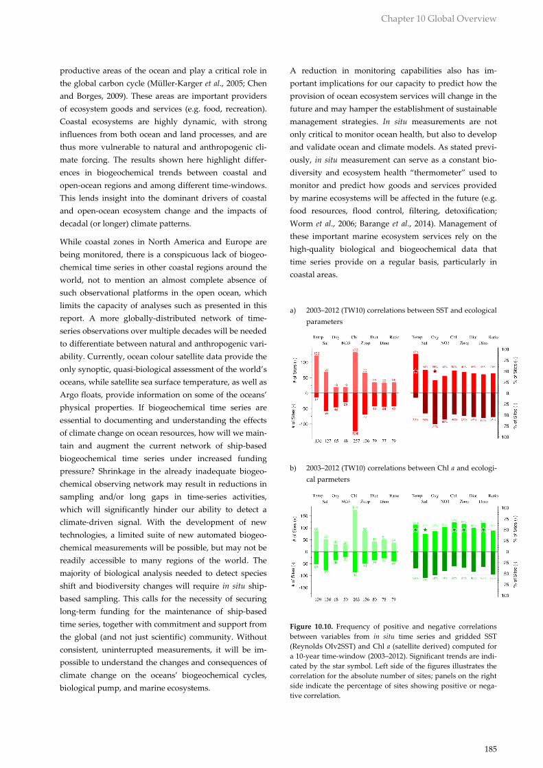
Figure 10.10. Frequency of positive and negative correlations

between variables from in situ time series and gridded SST

(Reynolds OIv2SST) and Chl a (satellite derived) computed for

a 10-year time-window (2003–2012). Significant trends are indi-

cated by the star symbol. Left side of the figures illustrates the

correlation for the absolute number of sites; panels on the right

side indicate the percentage of sites showing positive or nega-

tive correlation.

186

10.5 References

Alexander, M. A., Bladé, I., Newman, M., Lanzante, J. R.,

Lau, N-C., and Scott, J. D. 2002. The atmospheric

bridge: the influence of ENSO teleconnections on

air–sea interaction over the global oceans. Journal

of Climate, 15: 2205–2231,

doi:http://dx.doi.org/10.1175/1520-

0442(2002)015<2205:TABTIO>2.0.CO;2.

Arrigo, K. R., and van Dijken, G. L. 2011. Secular trends

in Arctic Ocean net primary production. Journal

of Geophysical Research, 116: C09011,

doi:10.1029/2011JC007151.

Bakun, A. 1990. Global climate change and intensifica-

tion of coastal ocean upwelling. Science,

247(4939): 198–201.

Barange, M., Merino, G., Blanchard, J. L., Scholtens, J.,

Harle, J., Allison, E. H., Allen, J. I., et al. 2014. Im-

pacts of climate change on marine ecosystem

production in societies dependent on fisheries.

Nature Climate Change, 4(3): 211–216,

doi:10.1038/NCLIMATE2119.

Barton, A. D., Irwin, A. J., Finkel, Z. V., and Stock, C. A.

2016. Anthropogenic climate change drives shift

and shuffle in North Atlantic phytoplankton

communities. Proceedings of the National Acad-

emy of Sciences, 113(11): 2964–2969.

Beaugrand, G., and Reid, P. C. 2003. Long-term changes

in phytoplankton, zooplankton and salmon

linked to climate. Global Change Biology, 9: 801–

817, doi:10.1046/j.1365-2486.2003.00632.x.

Beaulieu, C., Henson, S. A., Sarmiento, J. L., Dunne, J. P.,

Doney, S. C., Rykaczewski, R. R., and Bopp, L.

2013. Factors challenging our ability to detect

long-term trends in ocean chlorophyll. Biogeosci-

ences, 10: 2711–2724, doi:10.5194/bg-10-2711-2013.

Behrenfeld, M. J., O’Malley, R. T., Boss, E. S., Westberry,

T. K., Graff, J. R., Halsey, K. H., Milligan, A. J., et

al. 2015. Revaluating ocean warming impacts on

global phytoplankton. Nature Climate Change,

6(3): 323–330, doi:10.1038/NCLIMATE2838.

Behrenfeld, M. J., O’Malley, R. T., Siegel, D. A., McClain,

C. R., Sarmiento, J. L., Feldman, G. C., Milligan,

A. J., et al. 2006. Climate-driven trends in contem-

porary ocean productivity. Nature, 444(7120):

752–755.

Bopp, L., Aumont, O., Cadule, P., Alvain, S., and Gehlen,

M. 2005. Response of diatoms distribution to

global warming and potential implications: A

global model study. Geophysical Research Let-

ters, 32(19): L19606, doi:10.1029/2005GL023653.

Boyce, D. G. Lewis, M. R., and Worm, B. 2010. Global

phytoplankton decline over the past century. Na-

ture, 466(7306): 591–596, doi:10.1038/nature09268.

Brodie, J. E., and Mitchell, A. W. 2005. Nutrients in Aus-

tralian tropical rivers: changes with agricultural

development and implications for receiving envi-

ronments. Marine and Freshwater Research, 56:

279–302.

Caraco, N. F., and Cole, J. J. 1999. Human impact on ni-

trate export: an analysis using major world rivers.

Ambio, 28: 167–170.

Chavez, F. P., Messié, M., and Pennington, J. T. 2011.

Marine primary production in relation to climate

variability and change. Annual Review of Marine

Science, 3: 227–260.

Chavez, F. P., Ryan, J., Lluch-Cota, S. E., and Ñiquen, M.

2003. From anchovies to sardines and back: mul-

tidecadal change in the Pacific Ocean. Science,

299(5604): 217–221.

Chen, C. T. A., and Borges, A. V. 2009. Reconciling op-

posing views on carbon cycling in the coastal

ocean: continental shelves as sinks and near-shore

ecosystems as sources of atmospheric CO2. Deep-

Sea Research II: Topical Studies in Oceanography,

56(8): 578–590, doi:10.1016/j.dsr2.2009.01.001.

Church, M. J., Lomas, M. W., and Müller-Karger, F. 2013.

Sea change: Charting the course for biogeochemi-

cal ocean time-series research in a new millenni-

um. Deep-Sea Research II: Topical Studies in

Oceanography, 93: 2–15.

Dave, A. C., and Lozier, M. S. 2013. Examining the glob-

al record of interannual variability in stratification

and marine productivity in the low‐latitude and

mid‐latitude ocean. Journal of Geophysical Re-

search: Oceans, 118: 3114–3127,

doi:10.1002/jgrc.20224.

Deser, C., Phillips, A. S., and Alexander, M. A. 2010.

Twentieth century tropical sea surface tempera-

ture trends revisited. Geophysical Research Let-

ters, 37(10): L1070, doi: 10.1029/2010GL043321.

http://dx.doi.org/10.1038/nature09268

http://dx.doi.org/10.1002/jgrc.20224


187

Doney, S. C. 2006. Oceanography—Plankton in a warm-

er world, Nature, 444(7120): 695–696,

doi:10.1038/444695a.

Doney, S. C., Bopp, L., and Long, M. C. 2014. Historical

and future trends in ocean climate and biogeo-

chemistry. Oceanography, 27(1): 108–119,

http://dx.doi.org/10.5670/oceanog.2014.14.

Dong, L., and Zhou, T. 2014. The formation of the recent

cooling in the eastern tropical Pacific Ocean and

the associated climate impacts: A competition of

global warming, IPO, and AMO. Journal of Geo-

physical Research: Atmospheres, 119(19): 11272–

11287, doi:10.1002/2013JD021395.

Ducklow, H. W., Fraser, W. R., Meredith, M. P., Stam-

merjohn, S. E., Doney, S. C., Martinson, D. G.,

Sailley, S. F., et al. 2013. West Antarctic Peninsula:

An ice-dependent coastal marine ecosystem in

transition. Oceanography, 26(3): 190–203,

http://dx.doi.org/10.5670/oceanog.2013.62.

Enfield, D. B., and Mestas-Nuñez, A. M. 2000. Global

modes of ENSO and non-ENSO sea surface tem-

perature variability and their associations with

climate. In El Niño and the Southern Oscillation:

Multiscale Variability and Global and Regional

Impacts, pp. 89–112). Ed. by H. F. Diaz, and V.

Markgraf. Cambridge University Press. 512 pp.

Enfield, D. B., Mestas‐Nuñez, A. M., and Trimble, P. J.

2001. The Atlantic multidecadal oscillation and its

relation to rainfall and river flows in the continen-

tal US. Geophysical Research Letters, 28(10):

2077–2080.

Gao, K., Xu, J., Gao, G., Li, Y., Hutchins, D. A., Huang,

B., Wang, L., et al. 2012. Rising CO2 and increased

light exposure synergistically reduce marine pri-

mary productivity. Nature Climate Change, 2(7):

519–523.

García-Comasa, C., Stemmanna, L., Ibaneza, F., Berlinea,

L., Mazzocchi, M., Gasparinia, G. S., Picherala,

M., et al. 2011. Zooplankton long-term changes in

the NW Mediterranean Sea: Decadal periodicity

forced by winter hydrographic conditions related

to large-scale atmospheric changes? Journal of

Marine Systems, 87(3–4): 216–226.

Goffart, A., Hecq, J. H., and Legendre, L. 2002. Changes

in the development of the winter-spring phyto-

plankton bloom in the Bay of Calvi (NW Mediter-

ranean) over the last two decades: a response to

changing climate? Marine Ecology Progress Se-

ries, 236: 45–60, doi:10.3354/meps236045.

Gregg, W. W., and Rousseaux, C. S. 2014. Decadal trends

in global pelagic ocean chlorophyll: A new as-

sessment integrating multiple satellites, in situ da-

ta, and models. Journal of Geophysical Research:

Oceans, 119(9): 5921–5933.

Gruber, N. 2011. Warming up, turning sour, losing

breath: ocean biogeochemistry under global

change. Philosophical Transactions of the Royal

Society A, 369: 1980–1996,

doi:10.1098/rsta.2011.0003.

Han, W., Vialard, J., McPhaden, M. J., Lee, T., Masumo-

to, Y., Feng, M., and De Ruijter, W. P. 2014. Indian

Ocean decadal variability: A review. Bulletin of

the American Meteorological Society, 95(11):

1679–1703.

Henson, S. A. 2014. Slow science: the value of long ocean

biogeochemistry records. Philosophical Transac-

tions of the Royal Society A, 372(2025):

doi:10.1098/rsta.2013.0334.

Henson, S. A., Beaulieu, C., and Lampitt, R. 2016. Ob-

serving climate change trends in ocean biogeo-

chemistry: when and where. Global Change Biol-

ogy, 22(4): 1561–1571.

Henson, S., Cole, H., Beaulieu, C., and Yool, A. 2013. The

impact of global warming on seasonality of ocean

primary production. Biogeosciences, 10(6): 4357–

4369, doi:10.5194/bg-10-4357-2013.

Henson, S. A., Dunne, J., and Sarmiento, J. L. 2009. De-

cadal variability in North Atlantic phytoplankton

blooms. Journal of Geophysical Research, 114:

C04013, doi:10.1029/2008JC005139.

Henson, S. E., Sarmiento, J., Dunne, J., Bopp, L., Lima, I.,

Doney, S., John, J., et al. 2010. Detection of anthro-

pogenic climate change in the satellite records of

ocean chlorophyll and productivity. Biogeosci-

ences, 7: 621–640.

Hoegh-Guldberg, O., and Bruno, J. F. 2010. The impact

of climate change on the world’s marine ecosys‐

tems. Science, 328: 1523–1528.

http://dx.doi.org/10.1038/444695a

http://dx.doi.org/10.5670/oceanog.2013.62

188

Hoegh-Guldberg, O., Cai, R., Poloczanska, E. S., Brewer,

P. G., Sundby, S., Hilmi, H., Fabry, V. J., et al.

2014. The Ocean. In Climate Change 2014: Im-

pacts, Adaptation, and Vulnerability. Part B: Re-

gional Aspects, pp. 1655–1731. Ed. by V. R. Bar-

ros, C. B. Field, D. J. Dokken, M. D. Mastrandrea,

K. J. Mach, T. E. Bilir, M. Chatterjee, et al. Contri-

bution of Working Group II to the Fifth Assess-

ment Report of the Intergovernmental Panel on

Climate Change, Cambridge University Press,

Cambridge and New York. 688 pp.

Hurrell, J. W., and Deser, C. 2010. North Atlantic climate

variability: The role of the North Atlantic Oscilla-

tion. Journal of Marine Systems, 79 (3–4): 231–244.

IPCC. 2013. Climate Change 2013: The Physical Science

Basis. Contribution of Working Group I to the

Fifth Assessment Report of the Intergovernmental

Panel on Climate Change. Ed. by T. F. Stocker, D.

Qin, G-K. Plattner, M. Tignor, S. K. Allen, J.

Boschung, A. Nauels, et al. Cambridge University

Press, Cambridge and New York. 1535 pp.

Irwin, A. J., Nelles, A., M., and Finkel, Z. V. 2012. Phyto-

plankton niches estimated from field data. Lim-

nology and Oceanography, 57(3): 787–797,

doi:10.4319/lo.2012.57.3.0787.

Kamykowski, D., and Zentara, J. 1986. Predicting plant

nutrient concentrations from temperature and

sigma-t in the world ocean. Deep-Sea Research,

33: 89–105.

Kamykowski, D., and Zentara, J. 2005. Changes in world

ocean nitrate availability through the 20th centu-

ry. Deep-Sea Research I, 52: 1719–1744.

Karl, D. M. 2010. Oceanic ecosystem time-series pro-

grams. Oceanography, 23(3): 104–125.

Karl, T. R., Arguez, A., Huang, B., Lawrimore, J. H.,

McMahon, J. R., Menne, M. J., Peterson, T. C., et

al. 2015. Possible artifacts of data biases in the re-

cent global surface warming hiatus. Science,

348(6242): 1469–1472, doi:

10.1126/science.aaa5632.

Keeling, R. F., Körtzinger, A., and Gruber, N. 2010.

Ocean deoxygenation in a warming world. An-

nual Review of Marine Science, 2: 199–229.

Kempt, A. E., and Villareal, T. A. 2013. High diatom

production and export in stratified waters – A po-

tential negative feedback to global warming. Pro-

gress in Oceanography, 119: 4–23.

Knudsen, M. F., Seidenkrantz, M. S., Jacobsen, B. H., and

Kuijpers, A. 2011. Tracking the Atlantic Multide-

cadal Oscillation through the last 8,000 years. Na-

ture Communications, 2: 178.

Kosaka, Y., and Xie, S. P. 2013. Recent global-warming

hiatus tied to equatorial Pacific surface cooling.

Nature, 501(7467): 403–407.

Kwok, R., and Comiso, J. C. 2002. Spatial patterns of

variability in Antarctic surface temperature: Con-

nections to the Southern Hemisphere Annular

Mode and the Southern Oscillation. Geophysical

Research Letters, 29(14): 50-1–50-4,

doi:10.1029/2002GL015415.

Laws, E. A., Falkowski, P. G., Smith, W. O., Ducklow,

H., and McCarthy, J. J. 2000. Temperature effects

on export production in the open ocean. Global

Biogeochemical Cycles, 14(4): 1231–1246.

Lejeusne, C., Chevaldonné, P., Pergent-Martini, C., Bou-

douresque, C. F., and Pérez, T. 2010. Climate

change effects on a miniature ocean: the highly

diverse, highly impacted Mediterranean Sea.

Trends in Ecology & Evolution, 25(4): 250–260,

doi:http://dx.doi.org/10.1016/j.tree.2009.10.009.

Marshall, J., Armour, K. C., Scott, J. R., Kostov, Y.,

Hausmann, U., Ferreira, D., Shepherd, T. G., et al.

2014. The ocean's role in polar climate change:

asymmetric Arctic and Antarctic responses to

greenhouse gas and ozone forcing. Philosophical

Transactions of the Royal Society A, 372:

20130040, doi:10.1098/rsta.2013.0040.

Martiny, A. C., Pham, C. T. A., Primeau, F. W., Vrugt, J.

A., Moore, J. K., Levin, S. A., and Lomas, M. W.

2013. Strong latitudinal patterns in the elemental

ratios of marine plankton and organic matter. Na-

ture Geoscience, 6(4): 279–283,

doi:http://dx.doi.org/10.1038/ngeo1757.

Mazzocchi, M. G., Christoub, E. D., Di Capuaa, I., Fer-

nández de Puellesc, M., Fonda-Umanid, S., Mo-

lineroe, J. C., Nivalf, P., et al. 2007. Temporal vari-

ability of Centropages typicus in the Mediterranean

Sea over seasonal-to-decadal scales. Progress in

Oceanography, 72(2–3): 214–232,

doi:http://dx.doi.org/10.1016/j.pocean.2007.01.004.

Meredith, M. P., and King, J. C. 2005. Rapid climate

change in the ocean west of the Antarctic Penin-

sula during the second half of the 20th century.

Geophysical Research Letters, 32: L19604,

doi:10.1029/2005GL024042.


189

Meyer, J., and Riebesell, U. 2015. Reviews and syntheses:

Responses of coccolithophores to ocean acidifica-

tion: a meta-analysis. Biogeosciences, 12(6): 1671–

1682, doi:10.5194/bg-12-1671-2015.

Mills, M. M., and Arrigo, K. R. 2010. Magnitude of oce-

anic nitrogen fixation influenced by the nutrient

uptake ratio of phytoplankton. Nature Geosci-

ence, 3(6): 412–416.

Morel, A., Gentili, B., Claustre, H., Babin, M., Bricaud,

A., Ras, J., and Tieche, F. 2007. Optical properties

of the “clearest” natural waters. Limnology and

Oceanography, 52(1): 217–229.

McQuatters-Gollop, A., Reid, P. C., Edwards, M., Bur-

kill, P. H., Castellani, C., Batten, S., Gieskes, W., et

al. 2011. Is there a decline in marine phytoplank-

ton? Nature, 472(7342): E6–E7.

Müller-Karger, F. E., Varela, R., Thunell, R., Luerssen, R.,

Hu, C., and Walsh, J. J. 2005. The importance of

continental margins in the global carbon cycle.


doi:10.1029/2004GL021346.

Nobre, P., and Shukla, J. 1996. Variations of sea surface

temperature, wind stress, and rainfall over the

tropical Atlantic and South America. Journal of

Climate, 9: 2464–2479,


0442(1996)009<2464:VOSSTW>2.0.CO;2.

Overland, J. E., Alheit, J., Bakun, A., Hurrell, J. W.,

Mackas, D. L., and Miller, A. J. 2010. Climate con-

trols on marine ecosystems and fish populations.

Journal of Marine Systems, 79(3): 305–315.

Overland, J. E., Percival, D. B., and Mofjeld, H. O. 2006.

Regime shifts and red noise in the North Pacific.

Deep-Sea Research I: Oceanographic Research

Papers, 53(4): 582–588.

Polovina, J. J., Howell, E. A., and Abecassis, M. 2008.

Ocean's least productive waters are expanding.


doi:10.1029/2007GL031745.

Rahmstorf, S., Feulner, G., Mann, M. E., Robinson, A.,

Rutherford, S., and Schaffernicht, E. J. 2015. Ex-

ceptional twentieth-century slowdown in Atlantic

Ocean overturning circulation. Nature Climate

Change, 5(5): 475–480,

doi:10.1038/NCLIMATE2554.

Randel, W. J., and Wu, F. 1999. Cooling of the Arctic and

Antarctic polar stratosphere due to ozone deple-

tion. Journal of Climate, 12: 1467–1479,

doi:10.1175/1520-

0442(1999)012<1467:COTAAA>2.0.CO;2.

Richardson, A. J., and Schoeman, D. S. 2004. Climate

impact on plankton ecosystems in the Northeast

Atlantic. Science, 305(5690): 1609–1612,

doi:10.1126/science.1100958.

Richardson, A. 2008. In hot water: zooplankton and cli-

mate change. ICES Journal of Marine Science,

65(3): 279–295, doi:10.1093/icesjms/fsn028.

Riebesell, U., and Gattuso, J-P. 2015. Lessons learned

from ocean acidification research. Nature Climate

Change, 5(1): 12–14.

Riebesell, U., Schulz, K. G., Bellerby, R. G. J., Botros, M.,

Fritsche, P., Meyerhöfer, M., Neill, C., et al. 2007.

Enhanced biological carbon consumption in a

high CO2 ocean. Nature, 450(7169): 545–548.

Riebesell, U., and Tortell, P. D. 2011. Effects of ocean

acidification on pelagic organisms and ecosys-

tems. In Ocean Acidification, pp. 99–121. Ed. by J-

P. Gattuso, and L. Hansson. Oxford University

Press. 326 pp.

Serreze, M. C., and Barry, R. G. 2011. Processes and im-

pacts of Arctic amplification: A research synthe-

sis. Global and Planetary Change, 77(1–2): 85–96,

doi:http://dx.doi.org/10.1016/j.gloplacha.2011.03.0

04.

Siegel, D. A., Maritorena, S., Nelson, N. B., Behrenfeld,

M. J., and McClain, C. R. 2005. Colored dissolved

organic matter and its influence on the satellite-

based characterization of the ocean biosphere.


doi:10.1029/2005GL024310.

Siegel, D. A., Behrenfeld, M. J., Maritorena, S., McClain,

C. R., Antoine, D., Bailey, S. W., Bontempi, P. S., et

al. 2013. Regional to global assessments of phyto-

plankton dynamics from the SeaWiFS mission.

Remote Sensing of Environment, 135: 77–91.

Signorini, S. R., Franz, B. A., and McClain, C. R. 2015.

Chlorophyll variability in the oligotrophic gyres:

mechanisms, seasonality and trends. Frontiers in

Marine Science, 2: 1,

doi:10.3389/fmars.2015.00001.

http://dx.doi.org/10.1029/2007GL031745

190

Siokou-Frangou, I., Christaki, U., Mazzocchi, M. G.,

Montresor, M., Ribera d'Alcalá, M., Vaqué, D.,

and Zingone, A. 2010. Plankton in the open Medi-

terranean Sea: a review. Biogeosciences, 7, 1543-

1586.

Steig, E. J., Schneider, D. P., Rutherford, S. D., Mann, M.

E., Comiso, J. E., and Shindell, D. T. 2009. Warm-

ing of the Antarctic ice-sheet surface since the

1957 International Geophysical Year. Nature, 457:

459–462.

Sydeman, W. J., García-Reyes, M., Schoeman, D. S.,

Rykaczewski, R. R., Thompson, S. A., Black, B. A.,

and Bograd, S. J. 2014. Climate change and wind

intensification in coastal upwelling ecosystems.

Science, 345(6192): 77–80.

Thompson, D. W. J., and Solomon, S. 2002. Interpretation

of recent southern hemisphere climate change.

Science, 296(5569): 895–899,

doi:10.1126/science.1069270.

Vantrepotte, V., and Mélin, F. 2009. Temporal variability

of 10-year global SeaWiFS time series of phyto-

plankton chlorophyll a concentration. ICES Jour-

nal of Marine Science, 66(7): 1547–1556,

doi:10.1093/icesjms/fsp107.

Vantrepotte, V., and Mélin, F. 2011. Inter-annual varia-

tions in the SeaWiFS global chlorophyll a concen-

tration (1997–2007). Deep-Sea Research I: Ocean-

ographic Research Papers, 58(4): 429–441.

Venegas, S. A., Mysak, L. A., and Straub, D. N. 1997.

Atmosphere–ocean coupled variability in the

South Atlantic. Journal of Climate, 10: 2904–2920,


0442(1997)010<2904:AOCVIT>2.0.CO;2.

Visbeck, M. H., Hurrell, J. W., Polvani, L., and Cullen, H.

M. 2001. The North Atlantic Oscillation: Past, pre-

sent, and future. Proceedings of the National

Academy of Sciences of the United States of

America, 98(23): 12876–12877,

doi:10.1073/pnas.231391598.

Worm, B., Barbier, E. B., Beaumont, N., Duffy, J. E., Fol-

ke, C., Halpern, B. S., Jackson, J. B. C., et al. 2006.

Impacts of biodiversity loss on ocean ecosystem

services. Science, 314(5800): 787–790,

doi:10.1126/science.1132294.

Yu, L., Zhang, Z., Zhou, M., Zhong, S., Lenschow, D.,

Hsu, H., Wu, H., et al. 2012. Influence of the Ant-

arctic Oscillation, the Pacific–South American

modes and the El Niño–Southern Oscillation on

the Antarctic surface temperature and pressure

variations. Antarctic Science, 24(01): 59–76.

Yuras, G., Ulloa, O., and Hormazábal, S. 2005. On the

annual cycle of coastal and open ocean satellite

chlorophyll off Chile (18°–40°S). Geophysical Re-

search Letters, 32(23),

doi:http://dx.doi.org/10.1029/2005GL023946.

Zhang, J., Spitz, Y. H., Steele, M., Ashjian, C., Campbell,

R., Berline, L., and Matrai, P. 2010. Modeling the

impact of declining sea ice on the Arctic marine

planktonic ecosystem. Journal of Gephysical Re-

search, 115: C10015, doi:10.1029/2009JC005387.

http://dx.doi.org/10.1093/icesjms/fsp107

Documents

What are Marine Ecological Time Series telling us about ... · What are Marine Ecological Time Series telling us about the ocean? A status report [ Individual Chapter (PDF) download