Embed Size (px)
Citation preview
When Promotions Meet Operations:Cross-Selling and Its Effect on Call-Center Performance
We study cross-selling operations in call centers. The following question is addressed: How many
customer-service representatives are required (staffing)and when should cross-selling opportuni-
ties be exercised (control) in a way that will maximize the expected profit of the center while
maintaining a pre-specified service level target. We tacklethis question by characterizing control
and staffing schemes that are asymptotically optimal in the limit, as the system load grows large.
Our main finding is that a threshold priority (TP) control, inwhich cross-selling is exercised only if
the number of callers in the system is below a certain threshold, is asymptotically optimal in great
generality. The asymptotic optimality of TP reduces the staffing problem to a solution of a simple
deterministic problem, in one regime, and to a simple searchprocedure in another. We show that
our joint staffing and control scheme is nearly optimal for large systems. Furthermore, it performs
extremely well even for relatively small systems.
1. Introduction
Call Centers are in many cases the primary channel of interaction of a firm with its customers.
Historically, call centers were mostly considered a service delivery channel. Such service driven
call centers typically plan their operations based on delayrelated performance targets. Examples of
such performance measures are average speed of answer (ASA), the fraction of customers whose
call is answered by a certain time and the percentage of customer abandonment. These operational
problems have gained a lot of attention in the literature.
Most firms, however, cannot be considered to be purely service providers. Rather, customer ser-
vice is a companion to one or several main products. For example - the core business of computer
hardware companies, like Dell, is to sell computers. They do, however, have a call center whose
main purpose is to provide customer support after the purchase. Most banks have call centers that
give customer support while their main business is selling financial products. For these firms, the
inbound call center can be a natural sales channel. As opposed to outbound tele-marketing calls,
the interaction in the inbound call center is initiated by the customer. Once the customer calls the
center, a sales opportunity is generated. When the service part of the call is done, the agent might
choose to exercise this cross-selling opportunity by offering the customer an additional service or
product.
From a marketing point of view, a call center has a potential of becoming an ideal sales environ-
ment. Modern Customer Relationship Management (CRM) systems have dramatically improved
the information available to Customer Service Representatives (CSR’s) about the individual cus-
tomer in real time. Specifically, in call centers, once the caller has been identified, the CRM system
can inform the agent regarding this customer’s transactionhistory, her value to the firm and specific
cross-selling opportunities. As a result, cross-sales offerings can be tailored to the particular cus-
tomer, making modern call centers a perfect channel for customized sales. Many companies have
identified the revenue potential of inbound call centers. Indeed, as suggested by a McKinsey report
[11], call centers generate up to 25 percent of total new revenues for some credit card companies
and up to 60 percent for some telecom companies. Moreover, [11] estimates that cross-selling in a
bank’s call center can generate a significant revenue, equivalent to 10% of the revenue generated
through the bank’s entire branch network.
Although the benefits of running a joint service-and-sales call center are apparent, there are
various challenges involved in operating such a complex environment. An immediate implication
of incorporating sales is the increase in customer handlingtimes caused by cross-sales offerings.
Unless staffing levels are adjusted, the increased handlingtimes will inevitably lead to service
level degradation in terms of waiting times experienced by the customers. Does this imply that
incorporating cross-selling will necessarily lead to deterioration in service levels? What are the
appropriate operational tradeoffs that one should examinein the context of a combined service and
sales call center?
In a purely service driven call center, the manager typically attempts to minimize the staffing
level while maintaining a pre-determined delay-related performance target. Hence, in this pure
service context the operational tradeoff is clear: Staffingcost versus Service Level. When sales or
promotions are introduced, however, one should consider the potential revenue from these activities
as a third component of this tradeoff. Clearly, if the potential revenue is very high in comparison
to the staffing cost, it would be in the interest of the companyto increase the staffing level and
allow for as much cross-selling as possible. In these cases,increased revenues from cross-selling
need not come at the cost of service-level degradation. Rather, we show that the call center can
simultaneously achieve high cross-selling rates and very small waiting times. There are cases,
however, where the relation between staffing costs and potential revenues is more intricate and a
more careful analysis is required.
2
In addition to staffing, the dynamic control of incoming calls and cross-sales offerings is an-
other important component in the operations managements ofsuch centers. Specifically, the call
center manager needs to determine when the agent should exercise a cross-selling opportunity.
This decision should take into account not only the characteristics of the customer in service but
also the effect on the waiting times of other customers. For example, in order to satisfy a delay
target, it would be natural to stop all promotion activitiesin the presence of heavy congestion.
Indeed, a heuristic used in some call centers to determine when to exercise a cross-selling opportu-
nity, is to cross-sell upon service completion only when thenumber of callers in the queue is below
a certain threshold. Optimal rules, however, are typicallynot as simple. As cross-selling of a cus-
tomer can start only upon his service completion, an optimalcontrol is likely to use information
about whether the busy agents are providing service or are engaged in cross-selling. In particular, a
reduced state description that includes only information about the aggregate number of customers
in the system appears to be insufficient. In reality, however, the agents may not signal when they
move from the service phase of the interaction to the cross-selling phase and, consequently, it is
only the aggregate information that is available to the system manager. Hence, a control scheme
that relies on this information only is valuable in practice.
The staffing and control issues are co-dependent since even with seemingly adequate staffing
levels, the actual performance might be far from satisfactory when one does not make a careful
choice of the dynamic control. Yet, because of the complexity involved in addressing both issues
combined, they have been typically addressed separately inthe literature. To our knowledge, this
paper and its follow up paper [14] are the first to consider thestaffing and dynamic control in a
cross-selling environment jointly, in a single, common framework.
The purpose of this work is to carefully examine the major operational tradeoffs in the cross-
selling environment. This is done by specifying how to adjust the staffing level and how to choose
the control in order to balance staffing costs and cross-selling revenue potential while satisfying
quality of service constraints associated with delay performance. Specifically, we provide joint
staffing and dynamic control rules as explicit functions of the quality of service constraints, the
potential value of cross-selling and the staffing costs. Thecontrol we propose is a Threshold
Priority (TP) rule in which cross-selling is exercised onlywhen the number of callers in the system
is below a certain threshold. In contrast with the above-mentioned heuristic we identify cases in
which cross-selling should not be exercised even when thereare some idle agents in the system, in
anticipation for future arrivals.
To summarize, we contribute to the existing literature in a few dimensions:
3
1. From a modeling perspective, this is the first paper (together with our followup paper [14])
to address the staffing and cross-selling control questionsjointly in one single framework.
2. From a practical perspective - with the objective of maximizing profits while satisfying com-
monly used quality of service constraints - we propose a simple and practical Threshold Pri-
ority (TP) policy together with a staffing rule and rigorously establish their near-optimality.
(a) The qualities of the TP policy include:
i. It is based only on the total number of customers in the system, rather than the more
elaborate two-dimensional description that distinguishes between agents providing
service and those engaged in cross-selling.
ii. The simplicity of this policy has allowed us to significantly reduce the complexity
of the staffing problem.
(b) The staffing rule we propose is simple, easy to implement and reveals much about the
regime at which the center should operate: The Profit Driven (PD) versus the Service
Driven (SD) regime.
The rest of the paper is organized as follows: We conclude theintroductory part with a literature
review. §2 provides the problem formulation. In§3 we introduce the asymptotic framework and
state our key result: the asymptotic optimality of the threshold policy and the corresponding regime
driven staffing rule. A Markov Decision Process (MDP) approach to identify an optimal control
given any fixed staffing level is described and explored in§4. The solution of this MDP is used
as a benchmark in testing the performance of our asymptotic proposed scheme via an extensive
numerical study in§5. This section also explores implementation issues relevant for call center
managers.§6 concludes the paper with a discussion of our results and directions for future research.
A table of main notation is available immediately following§6.
For expository purposes, our approach in the presentation of the results is to state them formally
and precisely in the body of the paper, together with some supporting discussion, while relegating
the formal proofs to the technical appendix.
1.1 Literature Review
A successful and comprehensive treatment of cross-sellingimplementation in call centers would
clearly require an inter-disciplinary effort combining knowledge from marketing and operations
management as well as human resource management and information technology. An extensive
4
search of the literature shows, however, that while the marketing literature on cross-selling is quite
rich, very little has been done from the operations point of view (the reader is referred to Aksin
and Harker [1] for a survey of some of the marketing literature).
Although the operations literature on this subject is scarce, the topic of cross-selling has re-
ceived some attention. In the context of cross-selling in call centers, a significant contribution
is due to Aksin with various co-authors. In Aksin and Harker [1] the authors consider qualita-
tively and empirically the problems of cross-selling in banking call centers. They also suggest a
quantitative framework to evaluate the effects of cross-selling on service levels, using a proces-
sor sharing model, but they do not attempt to find optimal control or staffing levels.Ormeci and
Aksin [21], on the other hand, do pursue the goal of determining the optimal control, while as-
suming that the staffing level is given. In their framework, customers’ cross-selling value follows
a certain distribution. The realization of this value can beobserved by the call center before the
cross-selling offer is made. Hence, the agent can base the decision on the actual realization of this
value and not only its expected value. However, due to computational complexity, the results in
[21] are limited to multi-server loss systems (customers either hang-up or are blocked if their call
cannot be answered right away) and to structural results that are then used to propose a heuristic
for cross-selling. Gunes and Aksin [13] analyze the problem of providing incentives to agents in
order to obtain certain service levels and value generationgoals. This is indeed a critical issue in
cross-selling environments where the decision of whether to cross-sell or not is often made at the
discretion of the individual agents.
Simplicity of the dynamic control is clearly an important factor for a successful implementation
of cross-selling. The simplicity of the control might result, however, in decreasing revenues from
cross-selling. For example, it is intuitive that one can increase revenues by allowing the control to
be based on the identity of the individual customer in addition to the number of customers in the
system. Byers and So [9, 10] examine the value of customer identity information by comparing
cross-selling revenues under several control schemes thatdiffer with respect to the information
they use. Exact analysis is performed for the single server case in [10] and numerical results are
given for the multi-server case in [9].
To position our paper in the context of the literature introduced above, note that previous mod-
els have considered cross-selling decisions that are made upon customer assignment to an agent.
Our two-phase service model allows this decision to be postponed until the end of the service
phase when more information about the caller has been gathered. Another distinctive feature of
our model is our assumptions that the system operates with many-servers and an infinite buffer. In
5
contrast, single-server or loss-system assumptions are made in the existing literature for tractability
purposes. Also note that our paper is the first to consider howto optimally choose both the staffing
level and the control scheme in a cross-selling environment. If the staffing decision is ignored
and the staffing level is assumed to be fixed, the only relevanttradeoff is between service level
(expressed in terms of delay) and the extent to which cross-selling opportunities are exercised. In
this setting then, more cross-selling necessarily causes service level degradation. Moreover, the
existing literature suggests that, when the staffing level is assumed fixed, it is difficult to come up
with simple and practical control schemes for cross-selling. As we show in this paper, however,
when one adds the staffing component along with asymptotic analysis, the solution becomes sim-
pler. Indeed, our solution provides conditions under whichthe staffing level that maximizes the
expected profit from cross-selling simultaneously achieves extremely low waiting times.
In a follow-up paper [14], the authors use the results of the current paper to study the impact of
a heterogeneous pool of customers on the structure of asymptotically optimal staffing and control
schemes. [14] also investigates the value of customer segmentation in such an environment.
Our solution approach follows the many-server asymptotic framework, pioneered by Halfin
and Whitt [18]. In particular, we follow the asymptotic optimality framework approach first used
by Borst et al. [8], and adapted later to more complex settings ([3], [4], [5], [6], [15] and [19]).
The asymptotic regime that we use has been shown to be extremely robust even in relatively small
systems (see Borst et al. [8]); Consistent with this finding we give strong numerical evidence to
support the claim that this robustness is also typical in oursetting. We note however, that the
existing methods of establishing steady-state convergence in this asymptotic framework were not
sufficient for proofs in our framework. Instead, we introduce a proof methodology that was later
formalized in Gurvich and Zeevi [17] through the notion of Constrained Lyapunov Functions.
To conclude this review, we mention that, while outside the context of call centers, there is a
stream of operations management literature that deals withthe implications of cross-selling on the
inventory policy of a firm. Examples are the papers by Aydin and Ziya [7] and Netessine et. al.
[20].
2. Problem Formulation
We consider a call center with calls arriving according to a Poisson process with rateλ. An agent-
customer interaction begins with the service phase, whose duration is assumed to be exponentially
distributed with rateµs. Upon service completion, if cross-selling is exercised, this interaction will
6
enter a cross-selling phase, whose duration is assumed to beexponentially distributed with rate
µcs. If cross-selling is not exercised, either intentionally or due to the customer’s refusal to listen
to a cross-selling offer, the customer leaves the system. Itis assumed that all inter-arrival, service
and cross-selling times are independent and that the call center has an infinite waiting space.
Not all customers are viewed by the center as cross-selling candidates. We assume that the
customer population is divided into two segments so that only a fractionp of the customers are
potential cross-selling candidates. The remaining customers are not considered profitable and are
never cross-sold to. Whether or not a specific customer is a profitable candidate is interpreted
from a combination of the information available a-priori via the CRM system and the information
gathered by the agent during the interaction with the customer. It is important to note that, even
if an agent attempts to cross-sell to a caller, the latter will not necessarily agree to listen to the
cross-selling offer. We assume that a customer that is presented with the option to listen to a
cross-selling offer will agree to do so with probabilityq > 0. Assuming that all customers are
statistically identical, we have thatp = pq is the probability that a customer is a cross-selling
candidateandagrees to listen to the cross-selling offer if faced with one. The combined parameter
p is sufficient for our analysis so that we will not make additional references to the parameters
p and q. We assume that a cross-selling offer has an expected revenue of r, and revenues from
different customers are independent.
We say that a customer is in phase 1 of the customer-agent interaction if he is in the service
phase and in phase 2 if he is in the cross-selling phase. We usethe general notationπ for a
control policy that determines the actions in different decision epochs and, in particular, determines
whether or not to exercise this cross-selling opportunity upon a phase 1 completion of a cross-
selling candidate. We letZπi (t) be the number of servers providing phasei service at timet,
i = 1, 2 andZπ(t) = Zπ1 (t) + Zπ
2 (t) be the total number of busy agents at timet under the control
π. Given the number of agents,N , Iπ(t) := N − Zπ(t) is the number of idle agents at timet
under the controlπ. The number of customers waiting in queue at timet is denoted byQπ(t) and
Y π(t) is the overall number of customers in the system at timet (Y π(t) = Zπ(t)+Qπ(t)). Finally,
we letW π(t) be the virtual waiting time at timet (the waiting time that a virtual customer would
experience if s/he arrived at timet). In all of the above, we omit the time indext when referring
to steady-state variables. Also, we omit the superscriptπ whenever the control is clear from the
context. Note that under any stationary policy (as defined in[22, Page 22]), all transition rates in
the system can be determined using the number of agents busy providing either phase of service
and the queue length. In particular,Sπ(t) = {Zπi (t), i = 1, 2; Qπ(t)} is a Markov process under
7
any stationary policy. LetA(t) be the number of calls arriving by timet and letxπk , k = 1, 2, ...
be equal to1 if the kth arriving customer ends up going through phase2 and equal to0 otherwise.
Then, if steady-state exists underπ, we letP π(cs) be the long-run proportion of customers that go
through cross-selling, i.e,
P π(cs) := limt→∞
1
A(t)
A(t)∑
k=1
xπk ,
The control policyπ is picked from the following set of admissible controlsΠ(λ, µs, µcs, N).
Admissible Controls: Given a staffing levelN , and parametersλ, µs, µcs, we say thatπ is an
admissible policy if it is non-preemptive, non-anticipative and it weakly stabilizes the system1.
Non-anticipation should be interpreted here in the standard way; for a formal definition see e.g.
Definition 4.1 in [16]. In a nutshell, a policyπ is non-anticipative if a decision at a timet is only
based on the information revealed by the evolution of the system up to that time point. When the
parametersµs andµcs are fixed, we will omit them from the notation and use the notation Π(λ, N)
instead. The arrival rateλ and number of agentsN will also be omitted whenever their values are
clear from the context.
Finally, we note that by the PASTA property the steady-statevirtual waiting time and the
steady-state waiting time at arrival epochs coincide. WithC(·) being the staffing cost function,
the profit maximization formulation is then as follows:
maximize rλP π(cs) − C(N)
subject to E[W π] ≤ W ,
N ∈ Z+, π ∈ Π(λ, µs, µcs, N).
(1)
Here the average steady-state waiting timeE[W π] is constrained to be less than a pre-determined
boundW . We assume thatC(·) is convex increasing in the staffing levelN . Further assumptions
are made on the cost function in§3, where we construct our asymptotic framework. Note that
customers do not abandon, or balk, nor are they being blocked.2
One should note that we used the maximization formulation (1) although the maximum need
not exist. The word “maximize” should be formally interpreted as taking the supremum over all
staffing levels and admissible control policies.
1Weak-stability is defined aslimt→∞
E[Qπ(t)]t
= 0. For there to exist a policy that stabilizes the system we need,at the very least, thatλ/µs < N .
2As an alternative to the average-waiting-time constraint,one might consider the commonly used Quality of Service(QoS) constraint of the formP{W > W} ≤ δ. This stipulates that at least a fraction1 − δ of the customers will beanswered withinW units of time. One can verify that our analysis can be extended in a straightforward manner forconstraints of this form under the additional assumption that customers are served in a First Come First Served (FCFS)manner.
8
The following is an immediate consequence of Little’s Law and Markov Chain Ergodic theory.
Letting R := λ/µs be the offered (service) load we have that, for anyπ ∈ Π(λ, N) that admits a
steady-state distribution,
E[Zπ1 ] = R, (2)
and
λP π(cs) = µcs · E[Zπ2 ] = µcs · (E[Zπ] − R) ≤ µcs ·
[
(N − R) ∧ λp
µcs
]
, (3)
where for two real numbersx andy, x ∧ y = min{x, y}. Using observations (2) and (3), the
problem (1) may be re-written as
maximize rµcs(E[Zπ] − R) − C(N)
subject to E[W π] ≤ W ,
N ∈ Z+, π ∈ Π(N).
(4)
We now introduce the Threshold Priority (TP) control that will be shown to be nearly optimal
for (4) when combined with an appropriate staffing rule.
Definition 2.1 (The TP control) The Threshold Priority (TP) control is defined as follows:
(1) Upon customer arrival: An arriving customer enters service immediately if there are any
idle agents.
(2) Upon phase-1 completion:An agent that completes a phase 1 service with a customer at
a timet will exercise cross-selling if this customer is a cross-selling candidate and(Y (t) −N) ≤ K (whereK is a pre-determined integer).
(3) Upon customer departure: Upon a customer departure, the customer at the head of the
queue will be admitted to service if the queue is non-empty.
For brevity, we use the notationTP [K] to denoteTP with thresholdK (whereK may take neg-
ative as well as positive values). One should note the following: If K > 0, TP [K] is a control
that uses a threshold on the number of customers in queue. Specifically, upon service completion
with a cross-selling candidate, the agent will exercise cross-selling if the number of customers in
queue is at mostK. Conversely, ifK ≤ 0, TP [K] is a control that uses a threshold on the number
of idle agents. Specifically, upon service completion with across-selling candidate, the agent will
exercise cross-selling if the number of idle agents is at least |K|.
9
As TP [K] uses only information on the overall number of customers in the system at the time
of service completion, it is a stationary control. Furthermore, as TP disallows a positive queue
when there are idle agents, we have thatQ(t) = [Y (t)−N ]+ andZ1(t)+Z2(t) = N−[Y (t)−N ]−.
Hence, the evolution of the system–queue length, customer in service and customers in cross-
selling–is captured by the Markov processS(t) := {Z2(t), Y (t)}. Finally, we also establish that
TP is an admissible control (see Lemma F.1 in the appendix). Roughly speaking, the system
is stable under TP because of its self-balancing nature. Specifically, whenever the number of
customers in the system exceeds the levelK, all cross-selling activities are stopped. When this
happens, and asN > R, the system has sufficient capacity to provide service to allincoming calls.
We end this section with brief comments on our modeling assumptions.
Customers willingness to listen to a cross-selling offer:It is plausible that, in reality, the prob-
ability that a customer would be willing to listen to a cross-selling offer is not fixed, but rather
depends on the customer experience up to that point (such as his waiting time, service time, service
quality, etc.). This dependence introduces analytical complexity because the state space required
to describe such a system is very large (in particular, it would need to include for each customer
her current waiting time and service time). Given this complexity we assume in this paper that the
probability of agreeing to listen to a cross-selling offering is independentof the customer service
experience. This assumption is reasonable for systems in which waiting times are not too long and
service quality is uniformly good. The independence assumption is relaxed in Gurvich et al. [14]
where a cruder form of analysis is performed.
Even with the above simplifying assumption, the problem of optimally staffing and controlling
the call center requires keeping track of the two-dimensional processS(t) = {Z2(t), Y (t)}. The
two-dimensional structure makes the problem difficult to tackle with exact analysis. Instead, we
try to identify the structure of nearly optimal solutions via asymptotic analysis. This is the subject
of the next section.
3. Asymptotic Analysis
In this section we introduce the asymptotic framework and establish our asymptotic optimality
results. Consider a sequence of systems indexed by the arrival rateλ, which is assumed to grow
without bound (λ → ∞). The superscriptλ is used to denote quantities associated with theλth
system. We consider the following optimization problem which is obtained from (4) by adding the
10
dependence onλ where needed:
maximizeNλ,πλ
rµcs(E[Zλ,π] − R) − Cλ(Nλ)
subject to E[W λ,π] ≤ W λ
Nλ ∈ Z+, πλ ∈ Π(λ, Nλ),
(5)
Here and for the rest of the paper, we omit the superscriptλ from parameters that are not scaled with
λ, such as the service ratesµs andµcs, the expected revenue per customer,r, and the probability
p. The superscriptλ is also omitted fromR, sinceR has a trivial dependency onλ given by its
definition R = λ/µs. In terms of the cost functions, we consider convex increasing functions
Cλ(·) : R+ 7→ R+ with Cλ(0) = 0.
We define the scaling of the cost functions via a deterministic relaxation for (5). Specifically,
removing the waiting time constraint and replacingE[Zπ,λ] with a free decision variable, a deter-
ministic relaxation for the above problem is given
maximizeNλ,zλ
rµcs(zλ − R) − Cλ(Nλ)
subject to zλ ≤ Nλ,Nλ ≥ R,µcs(z
λ − R) ≤ λp,zλ ≥ 0, Nλ ∈ Z+.
(6)
The constraints in (6) follow from some basic observations.First, E[Zπ,λ] ≤ Nλ by definition.
Also, as we consider only staffing and control solutions thatmake the system stable, we must have
thatNλ ≥ R. Finally, the last constraint follows from (3).
Note that any optimal solution to (6) provides an upper boundon the optimal solution of (5).
Indeed, (6) is obtained from (5) by relaxing the restrictions on the waiting times and the fraction
of cross-sales. We also note that any optimal solution(z∗λ, N∗λ) to (6) hasz∗λ = N∗λ and, in
particular, the relaxation is equivalently given by
MaximizeNλ
rµcs · (Nλ − R) − Cλ(Nλ)
R ≤ Nλ ≤ R + λpµcs
Nλ ∈ R+.
(7)
The formulation (7) has a critical role in differentiating between the two operating regimes (see
discussion following (21)). For eachλ, let Nλ2 be thesmallestoptimal solution to (7). Then, we
make the following assumption:
Assumption 3.1
11
1. There existβ ≥ 0 andγ ∈ R, such that
limλ→∞
Nλ2 − R
R= β, and lim
λ→∞
Nλ2 − R(1 + β)√
R= γ. (8)
In particular,Nλ2 = R + βR + γ
√R + o(
√R).
2. There exists a ‘minimum wage’ parameterc > 0 such that for allλ and allN ≥ R,
Cλ(N) − Cλ(R) ≥ c(N − R).
Note that, by definition, we have thatNλ2 ≤ R + λp/µcs, and in particular thatβ ≤ µsp/µcs.
Assumption 3.1 is quite general in the sense that there is a large family of naturally occurring cost
functions that satisfy it. For example, any sequence of identical linear functions,Cλ(x) = cx,
for somec > 0, trivially satisfies this assumption. The same holds for a sequence of identical
convex functions. However, in order to consider a greater scope for our results, Assumption 3.1
also allows for functions that do scale withλ.
We impose the following assumption on the scaling of the waiting time constraint:
Assumption 3.2 There exists a constantW > 0, such that for allλ, W λ = W/√
R.
It is important to note that Assumptions 3.1 and 3.2 are not used in any way in the staffing and
control recommendation that we provide in Section 5. For these, one does not have to know the
constantsW , β, γ andc. Rather, the staffing and control will be given explicitly interms of cost
function C(·) and the waiting time targetW . The scaling in Assumption 3.2 is consistent with
many other models in which such square root approximations tend to perform extremely well (see
for example [15] and [8]).
Definition 3.1 Asymptotic Feasibility: We say that a sequence of staffing levels and controls
{Nλ, πλ} is asymptotically feasible, if when using{Nλ, πλ}, we have
lim supλ→∞
E[W λ]
W λ≤ 1. (9)
Let
V λ(Nλ, πλ) := rµcs(E[Zλ,π] − R) −(
Cλ(Nλ) − Cλ(R))
.
12
Definition 3.2 Asymptotic Optimality: We say that an asymptotically feasible sequence of staffing
levels and controls{Nλ, πλ} is asymptotically optimal if for any other asymptotically feasible
sequence{Nλ, πλ} we have
lim infλ→∞
V λ(Nλ, πλ)
V λ(Nλ, πλ)≥ 1. (10)
A natural notion of asymptotic optimality would stipulate that a sequence of pairs(Nλ, πλ) is
asymptotically optimal if it is asymptotically feasible and, for all λ large enough, it dominates any
other solution, i.e,
lim infλ→∞
rµcs(E[Zλ,πλ
] − R) − Cλ(Nλ)
rµcs(E[Zλ,πλ] − R) − Cλ(Nλ)≥ 1.
for any other asymptotically feasible sequence(Nλ, πλ). This notion, however, is too weak as it
implies that when the optimal solution involves cross-selling to a small fraction of the customers,
and, in particular, that
rµcs(E[Zλ,π] − R) = o(C(R)),
any staffing solution such thatNλ = R+o(R) with any reasonable control would be asymptotically
optimal. Yet, we would like to be able to differentiate between different staffing and control rules
even in cases when it is optimal to cross-sell to only a small fraction of the customers. Hence,
we normalize around the base cost ofC(R) which constitutes a lower bound on feasible staffing
levels.
Before stating our main asymptotic optimality result we need a few more definitions. Let
Nλ1 = min
{
N ∈ Z+ : E[W FCFSλ,µs
(N)] ≤ W λ}
. (11)
Then,N1 is the minimal number of servers required to meet the servicelevel target if no cross-
selling is performed and, in particular, it serves as a lowerbound on the number of servers required
in the system with cross-selling. Also, define
Nλ1 = min{N ∈ Z+, N ≥ R : E[W FCFS
λ,µs(N) |W FCFS
λ,µs(N) > 0] ≤ W λ}
= min{N ∈ Z+, N ≥ R :1
Nµs − λ≤ W λ}, (12)
where the last equality follows from the fact that, given wait, the waiting time in anM/M/N
queue with arrival rateλ and service rateµs has an exponential distribution with rateNµs −λ (see
e.g. §5-9 of Wolff [23]). Also, we will say that two sequences{xλ} and{yλ} satisfyxλ � yλ
13
if xλ/yλ → ∞ asλ → ∞. In the following theorem, then, we state the sufficient conditions for
asymptotic optimality of TP. For each condition we also specify how the staffing and the threshold
level will be determined if the condition is satisfied.
Theorem 3.1 Consider a sequence of systems, withλ → ∞, that satisfies Assumptions 3.1 and
3.2. Then, withNλ1 , Nλ
1 andNλ2 as defined in (11), (12) and (7) respectively, the following condi-
tions are sufficient for asymptotic optimality of TP and the proposed staffing levels:
1. Nλ2 − R � Nλ
1 − R, then it is asymptotically optimal to use any threshold valueKλ in the
interval [0, dλW λe] andNλ = Nλ2 .
2. Condition 1 fails butlim infλ→∞Nλ
2 −R
Nλ1 −R
≥ 1, andµcs ≥ µs, then it is asymptotically optimal
to setKλ = 0 andNλ = Nλ2 .
3. µs = µcs and lim supλ→∞Nλ
2 −R
Nλ1 −R
< 1, then it is asymptotically optimal to setNλ = N∗λ
andKλ = K∗λ, whereK∗λ := Kλ(N∗λ) andN∗λ are determined by choosing the smallest
value ofN∗λ that satisfies
N∗λ := arg maxN≥Nλ1{ rµcs(E
[
ZFCFSλ,µs
(N) |ZFCFSλ,µs
(N) ≥ (N + Kλ(N)) ∧ N]
− R)
−(Cλ(N) − Cλ(R))},(13)
whereKλ(N) in (13) satisfies
Kλ(N) := maxK≥−N
{E[QFCFSλ,µs
(N) |ZFCFSλ,µs
(N) ≥ (N + K) ∧ N ] ≤ λW λ}. (14)
Under Condition 1, the value of cross-selling drives the system to use a significant amount of extra
staffing to allow for substantial cross-selling. Hence, whenever this condition is satisfied, we say
that the system operates in theProfit Driven Regime.In contrast, whenever Conditions 2 or 3 hold,
the fraction of customers experiencing cross-selling is relatively small. Under Condition 2 staffing
is still determined by profit considerations, and the systemis still considered to be operating in the
Profit Driven regime. Under Condition 3, the focus of the staffing becomes the satisfaction of the
quality of service constraint. In that case, we say that the system operates in theService-Driven
Regime. This regime characterization is further discussed in§5 where we provide prescription
towards the practical implementation of a staffing and cross-selling rule.
14
4. The MDP Approach
When either of the Conditions 1, 2 or 3 in Theorem 3.1 is satisfied, we managed to overcome
the two-dimensional nature of the control problem through our asymptotic analysis, and show that
our proposed scheme that combines a TP threshold control with a regime-based staffing rule is
asymptotically optimal. But how well does this scheme perform for a call center of a moderate
size? How well does it perform if neither of the sufficient conditions of Theorem 3.1 holds? To
address these questions, in this section, we propose a solution approach to the control component
of (1) which applies in great generality, beyond the cases covered by Theorem 3.1. Specifically,
following the approach in [12], we consider the solution to arelatedMarkov Decision Process
(MDP). First, we truncate the state-space to reduce the infinite-state-space problem into a finite
dimensional one. Specifically, we solve the MDP for afinite buffersystem and show that the
optimal solution to the finite-state-space MDP converges tothe optimal solution of the original
problem, as the buffer size grows without bound. This finite buffer MDP is solved through a
solution to a linear program (LP). The optimal control associated with the solution to the LP is
generally not a TP control. Nevertheless, in§5 we show that TP is nearly optimal by numerically
comparing its performance to that of the optimal control obtained from the solution of the LP. Note
that in this section,λ is fixed and is omitted as a superscript from all notation.
We now turn to the formulation of the Markov Decision Processand its reduction to a solu-
tion of an LP. We start by showing that it suffices to consider asubset of all admissible policies.
Specifically, in Lemmas 4.1 and 4.2 we show that, if there exists an optimal control, then there
always exists one that iswork conservingand serves customersFCFS. For a fixedN , we re-define
Π(N) to be the set of non-anticipative non-preemptivefeasiblepolicies. That is, given a staffing
levelN ∈ Z+, Π(N) consists of all policiesπ for which (together withN) steady state exists and
E[W π] ≤ W . In particular, it is clear thatΠ(N) will be empty unlessN ≥ N1, whereN1 is
defined in (11).
Lemma 4.1 Fix λ, µs, µcs andN . Then, for anyπ ∈ Π(N) there exists a policyπ′ ∈ Π(N) that
serves customers FCFS and performs at least as well asπ. In particular,π′ admits a cross-selling
rate that is at least as large as that admitted byπ.
Definition 4.1 Work Conservation:We say that a policyπ is work conserving if: (i) whenever
a customer arrives to find an idle agent, s/he is immediately admitted to service, and (ii) upon
15
a departure of a customer from the system, a waiting customerwill be admitted to service if the
queue is non-empty.
Note that work conservation implies thatZ(t) = N wheneverQ(t) > 0. It does not imply,
however, that the policy gives priority to the customers waiting in queue over cross-selling. In fact,
work conservation does allow exercising cross-selling even when customers are waiting.
The following lemma shows that within the class of FCFS policies it is sufficient to consider
work conserving policies. In turn, it suffices to consider FCFS work conserving policies.
Lemma 4.2 Fix λ, µs, µcs andN . Then, for any feasible policyπ ∈ Π(N) that serves customers
FCFS, there exists a work conserving feasible policyπ′ ∈ Π(N) that performs at least as well as
π and serves customers FCFS. In particularπ′ admits a cross-selling rate that is at least as large
as that admitted byπ.
Within the set of work conserving FCFS policies we limit our attention to stationary policies.
Stationary policies are practical, and are typically optimal. Their optimality has not been estab-
lished in general in a setting with infinite state space. Thus, we impose the restriction to stationary
policies as an assumption and re-define the set of admissiblepoliciesΠ(N) accordingly.
Admissible Policies: For a fixedN , the admissible policiesΠ(N) is the set of non-anticipative,
non-preemptive,stationary, work-conserving, FCFS, feasible policies.
Note that Lemmas 4.1 and 4.2 prove that the family of work conserving FCFS policies is
optimal, but we have not established that the family ofstationarywork conserving FCFS policies
is optimal. Instead, we henceforth restrict our attention to this new set of admissible policies as
defined above.
We are now ready to construct the MDP and the associated Linear Program for a cross-selling
system with afinite buffer. We will later prove that, for a buffer size that is large enough, and for
any given admissible policy for the infinite buffer system, there exists a stationary work conserving
and FCFS policy for the finite buffer system that performs almost as well. This implies that the
optimal solution of the constructed LP converges to an optimal solution of the original problem.
For stationary work-conserving FCFS policies, the state descriptor{Z2(t), Y (t)} suffices for a
complete Markovian characterization of the system. Indeed, work conservation implies that the
identitiesZ1(t) = (Y (t) ∧N)−Z2(t) andQ(t) = [Y (t)−N ]+ hold, so that one can characterize
the behavior of the whole system through the two-dimensional description{Z2(t), Y (t)}. Suppose
16
that the number of customers in system is bounded above by a finite number of trunk lines,L ≥ N .
Customers that find a full buffer upon arrival are blocked anddo not enter the system.
Since all transition rates in the system are bounded byλ + Nµs + Nµcs we can replace the
analysis of the underlying Continuous Time Markov Chain (CTMC) with the analysis of the associ-
ated Discrete Time Markov Chain (DTMC) which is obtained from the CTMC by uniformization.
The construction by uniformization ensures that the steady-state fraction of time that the CTMC
spends in any given state corresponds exactly to the fraction of steps that the corresponding DTMC
spends in that state under its stationary distribution; seee.g. [22, pp. 562-563]. Naturally, we let
the uniformization rate equal the upper boundλ + Nµs + Nµcs.
By results for constrained long run-average MDP’s (see for example section 4.2 of [2]) one can
solve the finite state MDP through an appropriate LP. Note that due to work conservation, in each
state{Z2, Y } the action set consists of only two options - cross sell upon service completion (1) or
do not cross-sell (0). Letξ(i, j, k) be the steady-state probability of being in state{Z2, Y } = (i, j)
and taking the actionk ∈ {0, 1} (note that a stationary distribution will always exist for this model
due to the finite buffer). The corresponding LP for a system with L trunk lines andN agents is
given by:
Max∑L
j=0
∑j∧Ni=0 riµcs(ξ(i, j, 0) + ξ(i, j, 1)) (15)
s.t (λ + Nµs + Nµcs) · (ξ(i, j, 0) + ξ(i, j, 1)) = λ(ξ(i, j − 1, 0) + ξ(i, j − 1, 1))1{j−1≥0}
+µs((j + 1) ∧ N − i) (ξ(i, j + 1, 0) + (1 − p)ξ(i, j + 1, 1)) 1{j+1≤L}
+pµs(j ∧ N − (i − 1))ξ(i− 1, j, 1)1{i−1≥0}
+µcs(i + 1)(ξ(i + 1, j + 1, 0) + ξ(i + 1, j + 1, 1))1{i+1≤N}1{j+1≤L}
+(ξ(i, j, 0) + ξ(i, j, 1))(
(N − i)µcs + (N − (j ∧ N − i))µs + λ1{j=L})
,
0 ≤ j ≤ L, 0 ≤ i ≤ j ∧ N,(16)
L∑
j=0
j∧N∑
i=0
(ξ(i, j, 0) + ξ(i, j, 1)) = 1, (17)
andL∑
j=N
(j − N)
N∑
i=0
(ξ(i, j, 0) + ξ(i, j, 1)) ≤ λW (18)
The system of equations in (16) represents the balance equations of the underlying DTMC, keep-
ing in mind that the action choice only affects the chain transitions immediately following a phase
1 service completion. In particular, for any fixed(i, j) the right hand side in (16) lists the possible
17
transitions from other states into(i, j, 0) and(i, j, 1), with the corresponding probabilities. Specif-
ically, the first line on the right hand side of (16) corresponds to transitions due to arrivals. The
second line corresponds to transitions due to phase 1 service completions that are not followed by
a cross-selling phase. The third line corresponds to transitions due to phase 1 service completions
that are followed by cross-selling. The fourth line corresponds to transitions due to phase 2 service
completions and the last line corresponds to transitions from the state to itself.
Recall that any feasible staffing level for the original system (with infinite number of lines)
must be greater than or equal toN1 where
N1 = arg min{
N ∈ Z+ : E[W FCFSλ,µs
(N)] ≤ W}
. (19)
Let V ∗LP (N, L) be the optimal solution of the LP corresponding to a system with N agents
andL trunk lines (recall thatλ is fixed). For a fixedN , let V ∗(N) be the optimal expected profit
in (4), that is
V ∗(N) = supπ∈Π(N):E[W π]≤W
rµcs(E[Zπ] − R).
Then, we have the following:
Proposition 4.1 AssumeN ≥ N1. Then,
limL→∞
V ∗LP (N, L) = V ∗(N). (20)
We use the result of Proposition 4.1 in the next section to illustrate the good performance of
TP. Specifically, we show numerically that TP achieves a cross-selling rate that is almost identical
to the one obtained through the LP with a large buffer size. This indicates that, within the set of
stationary work-conserving FCFS policies, TP is close to optimal.
5. Discussion of Implementation and Performance Analysis
In this section we interpret the results of the asymptotic analysis in§3 to come up with a practical
staffing and cross-selling prescription for call centers. We validate our prescription through nu-
merical examples in which we compare the performance of our recommended policy with that of
the optimal policy found via the explicit solution of the corresponding Markov Decision Process
(MDP) problem with a large enough buffer size.
18
5.1 Prescription for Implementation
Our asymptotic optimality suggests that a TP control together with a proper staffing rule should
perform close to optimality under a set of sufficient conditions as listed in Theorem 3.1. In those
cases, the TP rule offers significant simplifications towards the solution of the original problem.
The results in Theorem 3.1 are, however, given in asymptoticterms (for sequences of systems)
and it is not a-priori clear how to verify that the conditionshold for a given system. Moreover, it
is of interest to examine the performance of our proposed policy when the conditions of Theorem
3.1 do not hold. In these cases, the simplicity of the TP rule allows us to construct simple search-
based procedures and compare them to the performance of the optimal solution in cases that are
not covered by Theorem 3.1.
First, we note that a key understanding from our asymptotic analysis is the distinction between
the Profit Driven and the Service Driven regimes. LettingN2 be a staffing level that solves the
optimization problem:Maximize rµcs(N − R) − C(N),
s.t. R ≤ N ≤ R + λpµcs
,
N ∈ R+,
, (21)
we showed that whenever
N2 − R � N1 − R, (22)
it is nearly optimal to staff withdN2e agents and useTP [K], with anyK ∈ [0, dλWe]. Here,N1 is
as defined in (11). The question is when is it reasonable to saythat (22) holds. Our rule-of-thumb
for regime characterization says that the Profit Driven regime is the correct regime provided that
there existsx > 0 such thatC ′(R(1 + y)) < rµcs for all y ∈ [0, x]. (23)
In words, (23) implies that the marginal capacity cost is less than the maximum potential marginal
revenue from adding a server (rµcs). In particular, we expect that in this case the optimal staffing
levelN2 in (21) will satisfyN2 >> R. Moreover, if the functionC(·) is convex, we will have that
N2 = inf{x ≥ R : C ′(x) ≤ rµcs}.
Above we have implicitly assumed that the derivative exists, but if not (as staffing levels are
discrete) the regime condition (23) can be re-written as
there existsx > 0 such thatC(R(1 + y)) − C(R(1 + y) − 1) < rµcs for all y ∈ [0, x].
Theorem 3.1 shows that, if (23) holds, the call center can obtain profit that is almost as high as
the one that could be obtained in the absence of any service level considerations. Hence, whenever
19
(22) holds, the staffing decisions are essentially driven bythe profit rather than by the service-level
constraint. Even if (22) does not hold, the staffing levelN2 may still be nearly optimal provided
that
N2 ≥ N1 := inf{N ∈ Z+, N ≥ R :1
Nµs − λ≤ W}, (24)
and we have fast cross-selling, i.e,µcs ≥ µs. In this case, Theorem 3.1 shows that it is nearly
optimal to useN2 with TP [K] with K = 0.
In some cases, the revenue from cross-selling is not high enough to justify staffing that is sig-
nificantly above the basic staffing needed for service-levelsatisfaction (without cross-selling). In
such cases, more care is needed and the optimal staffing levelis more sensitive to the service-level
targetW . This is the Service-Driven regime which is characterized by the conditionN2 ≤ N1. In
these cases, even nearly optimal staffing and control solutions do not necessarily exhibit the decou-
pling between profit and service-levels observed in the PD regime. Hence, it is a more challenging
regime to handle. Whenever the service and cross-selling rates are equal (µs = µcs =: µ), Theorem
3.1 shows that it is asymptotically optimal to useN∗ for staffing andTP with thresholdK(N∗)
for cross-selling, withN∗ andK(N∗) chosen as in (13) and (14). Thus, when the service-rates
are equal, while the underlying dynamics are still complex,we are able to derive a nearly optimal
solution. The example depicted in Figure 4 (in§5.2) numerically illustrates the regime separation.
When the sufficient conditions of Theorem 3.1 do not hold the simplicity of the TP based rule
still allows one to use a simple search-based procedure to determine the threshold and the staffing
level. Indeed, focusing on a threshold control only, reduces the problem into a simple search
over these two parameters, where for each pair(N, K) performance measures may be obtained by
computing the steady-state distribution or via simulation. While the result is not provably optimal
we will show numerically that it performs extremely well. Indesigning the search procedure, we
use the following observations: First, it suffices to consider staffing levels that satisfyN ≥ N1.
Second, from Theorem 3.1, we know that it suffices to considerstaffing levelsN such thatN ≤R + λp/µcs. Indeed, by definition we have thatN2 ≤ R + λp/µcs and we know thatN2 is nearly
optimal if (22) holds. Finally, Theorem 3.1 shows that for near optimality it suffices to consider
threshold valuesK ∈ [−N, dλW e]. Hence, the search procedure we propose is as follows:
1. SetN = N1. SetVmax = −(C(N1) − C(R)).
2. WhileN ≤ dR + λp/µcse:
(a) SetK = dλW e
20
(b) whileK ≥ −N :
i. EvaluateE[W ] andµcs(E[Z]−R) (by simulation or by solving the balance equa-
tions).
ii. If E[W ] ≤ W :
A. If rµcs(E[Z] − R) − C(N) − C(R) > Vmax, setN∗ = N andK(N∗) = K.
B. SetN = N + 1 and go to back to 2.
iii. If E[W ] > W , setK = K − 1 and go back to (b).
To summarize, we provide the following implementation prescription:
i. If (23) holds, then usedN2e for staffing and useTP [K] for cross-selling, with anyK ∈[0, dλWe].
ii. If cross-selling is faster, on average, than service (µcs ≥ µs) and (24) holds, then usedN2efor staffing and useTP [K] for cross-selling, withK = 0
iii. If (24) does not hold butµs = µcs, useN∗ andK(N∗) as determined by (13) and (14),
respectively.
iv. In all other cases, perform the search procedure above.
Of course, relying on the search procedure in the cases in which the conditions of Theorem
3.1 do not hold, has no performance guarantees. The remainder of this section is dedicated to
a detailed numerical study of the performance of our proposed two-parameter search procedure.
Particularly, we demonstrate that our scheme performs extremely well, even when it is notprovably
nearly-optimal.
5.2 Performance Evaluation
This section is divided to two parts. First, we analyze the performance of the TP rule for different
(but fixed) staffing levels. This part can be regarded as dealing with the problem of finding optimal
cross-selling policies for given staffing levels. In the second part we address the joint staffing-
and-control problem and, in the process, provide numericalsupport for the distinction between the
Profit Driven and the Service Driven regimes. In both parts wecompare the resulting performance
against that of the optimal solutions (among all stationarywork-conserving FCFS policies) as
found via the explicit solution of the associated MDP with a large enough buffer size.3
3In each example we increased the buffer size until the point where the effect on the profits was negligible. Wefound that a buffer size of100 was sufficient for most examples.
21
Performance of TP for given staffing levels: Here we compare the value obtained through the
solution of the original optimization problem via MDP versus the performance obtained using TP.
We show that TP performs well beyond the scope covered by our sufficient conditions and that it
exhibits good performance also in relatively small call centers. We experiment with two different
call centers. The first, with an offered load ofR = 30, representing a relatively small call center.
The second, with an offered load ofR = 100, representing a medium-size call center. We assume
that the service-level constraint is given byE[W ] ≤ 0.1/µs which, in a setting with a mean service
time of 5 minutes, corresponds to an upper bound of 30 secondson the average waiting time. We
fix µs = 1 throughout but allow for different ratios ofµcs/µs, ranging from0.1 to 10 where the
extreme casesµcs = 0.1 andµcs = 10 represent very slow cross-selling and very fast cross-selling,
respectively. In all the experimentsr is assumed to be 1, so that the expected cross-selling revenue
is essentially equal to the cross-selling rate. We will initially assume also thatp = 1 but later
(Figure 3) we consider values ofp < 1.
We use equation (11) to findN1, the least number of servers that is required to satisfy the service
level in the absence of any cross-selling activity. We find thatN1 = 34 for R = 30, andN1 = 106
for R = 100. We then vary the staffing level,N , in steps of4 in the range{N1, . . . , N1 + 40}.
The range of staffing levels that we examine is large enough tocover both operating regimes and a
wide range of optimal thresholds – that are both negative when in the SD regime (see below) and
positive when the staffing levels are sufficiently greater thanN1.
The experiments then proceed as follows: for each value ofµcs andN we find the revenue under
TP and the revenue obtained from the optimal solution of the MDP. For the former, givenµcs and
N , we fix the policy to be TP but vary the threshold,K, using two methods: a) using our search
procedure described in§5.1 (note that this search is limited toK ∈ [−N, dλW e]) , and b) by an
exhaustive search to find the threshold that maximizes the revenue among all possible thresholds.
For each combination ofµcs, N andK, the revenue and the queue length are calculated by solving
the balance equations of the Continuous Time Markov Chain (CTMC), S(t) := {Z2(t), Y (t)}.
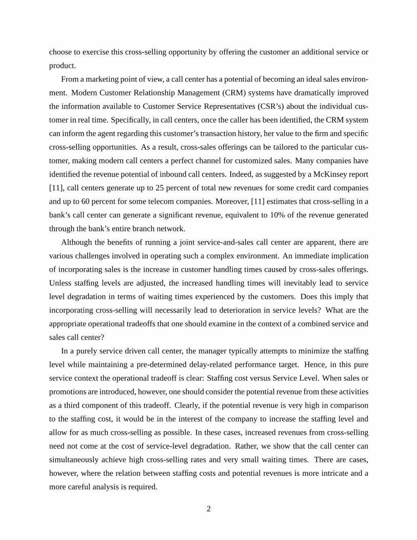
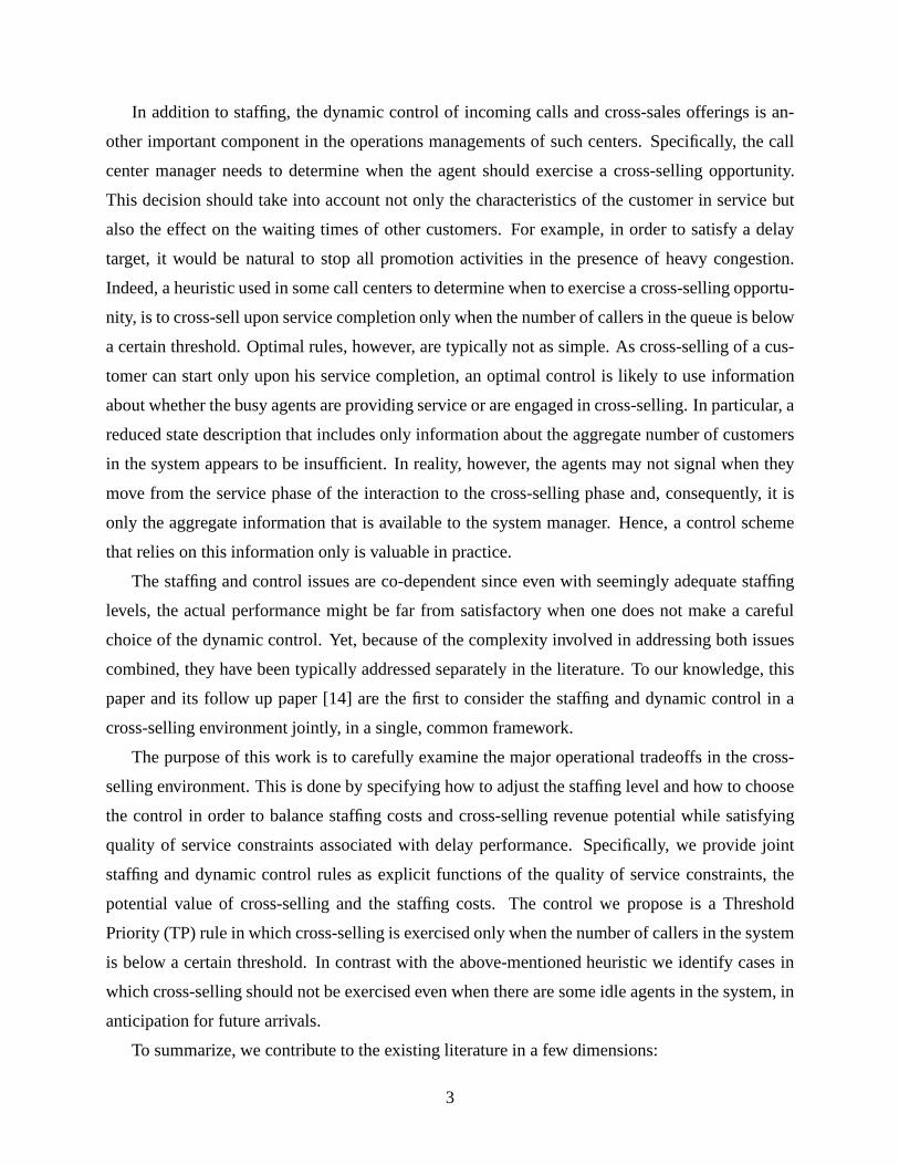
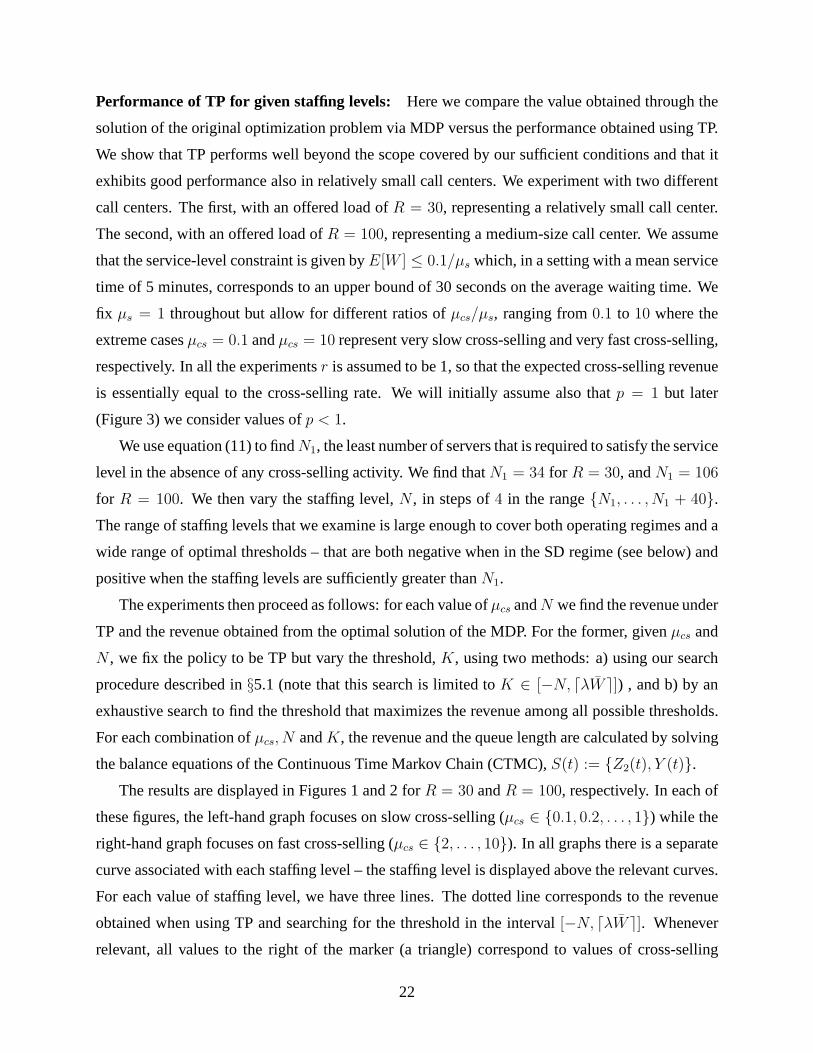
The results are displayed in Figures 1 and 2 forR = 30 andR = 100, respectively. In each of
these figures, the left-hand graph focuses on slow cross-selling (µcs ∈ {0.1, 0.2, . . . , 1}) while the
right-hand graph focuses on fast cross-selling (µcs ∈ {2, . . . , 10}). In all graphs there is a separate
curve associated with each staffing level – the staffing levelis displayed above the relevant curves.
For each value of staffing level, we have three lines. The dotted line corresponds to the revenue
obtained when using TP and searching for the threshold in theinterval [−N, dλW e]. Whenever
relevant, all values to the right of the marker (a triangle) correspond to values of cross-selling
22
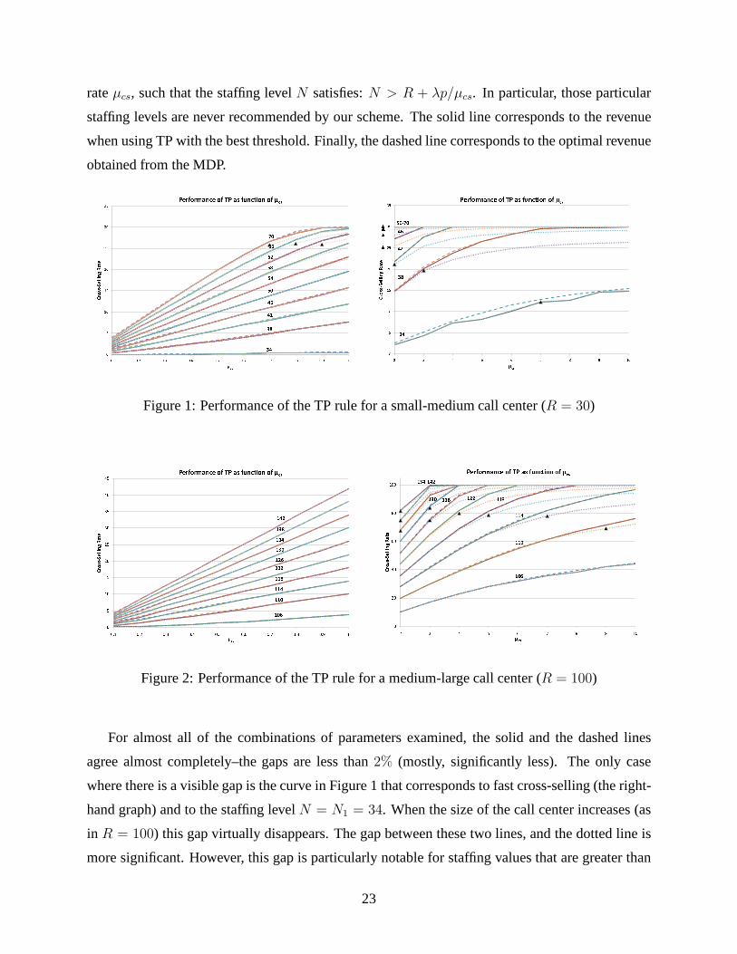
rateµcs, such that the staffing levelN satisfies:N > R + λp/µcs. In particular, those particular
staffing levels are never recommended by our scheme. The solid line corresponds to the revenue
when using TP with the best threshold. Finally, the dashed line corresponds to the optimal revenue
obtained from the MDP.
��� �� �� �� �� �� �� � � � � � � � � � � � � � � � � � � � � � � � � �� � �� �� ���� ��� �� �
� � �� � � � � ! " # $ � � % � " & � ' # $ ( ) # � * + ,
- .- /. 01 2. 31 .1 /3 03 34 2567 57 68 58 69 59 6
8 9 : 6 ; < = > 7 5? @ABB CD EFFG HIJ KL EM N O
P Q R S T R U V W X Q T S Y P V Z S [ W X \ ] T W T S ^ _ `a ba cb de f g h fb ijjjj
Figure 1: Performance of the TP rule for a small-medium call center (R = 30)
klm km ln kn lo ko lp kp lk q m k q n k q o k q p k q l k q r k q s k q t k q u mv wxyy z{ |}}~ ��� �� |
� � �� � � � � � � � � � � � � � � � � � � � � � � � � � � � � �
� � �� � �� � �� � �� � �� � �� � �� � �� � �� � �� �¡ �¢ �£ �¤ � �
¥ ¡ ¦ ¢ § £ ¨ ¤ �© ª«¬¬ ® ¯°°± ²³´ µ¶ ¯· ¸ ¹
º » ¼ ½ ¾ ¼ ¿ À Á Â » ¾ ½ Ã º À Ä ½ Å Á Â Æ Ç ¾ Á ¾ ½ È É ÊË Ì ÍË Ë ÌË Ë ÎË Ï Ï Ë Ë ÐË Ï ÍË Ñ ÌË Ñ Î Ò Ë Î Ï
Figure 2: Performance of the TP rule for a medium-large call center (R = 100)
For almost all of the combinations of parameters examined, the solid and the dashed lines
agree almost completely–the gaps are less than2% (mostly, significantly less). The only case
where there is a visible gap is the curve in Figure 1 that corresponds to fast cross-selling (the right-
hand graph) and to the staffing levelN = N1 = 34. When the size of the call center increases (as
in R = 100) this gap virtually disappears. The gap between these two lines, and the dotted line is
more significant. However, this gap is particularly notablefor staffing values that are greater than
23
R+λp/µcs – these are staffing values that our scheme does not recommendusing. This underlines
the importance of jointly solving for the staffing and control problems. If staffing is determined
according to our proposed rule, threshold values may be restricted to the interval[−N, dλW e]. If
staffing levels are beyond the recommended range a full search over all possible threshold values
is needed.
The case ofR = 100 also serves to emphasize another important point. In the introduction
we mention that using a threshold on the queue length is a common heuristic, i.e, cross-selling is
exercised upon service completion only when the number of callers in thequeueis below a certain
threshold. Examining the optimal thresholds generated forthis example through our numerical
analysis reveals the need to use thresholds on thenumber of idle agentsin some cases (as allowed
by TP by settingK < 0), rather than on the number of customers in queue. Focusing on the case
R = 100 andµcs = 1/3, the optimal thresholds for the different staffing levels are given in Table
1 which shows that, for all staffing levels,106− 122, the optimal threshold is negative. Intuitively,
it is optimal to have a threshold on the number of idle agents whenever the waiting time constraint
will otherwise be violated. In particular, if staffing levelis sufficiently low, one has to reserve idle
agents for future arriving calls, in order to satisfy feasibility.
Staffing 106 110 114 118 122 126 130 136 142Threshold -20 -10 -6 -3 -1 1 2 3 4
Table 1: Threshold values forR = 100
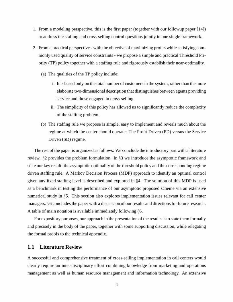
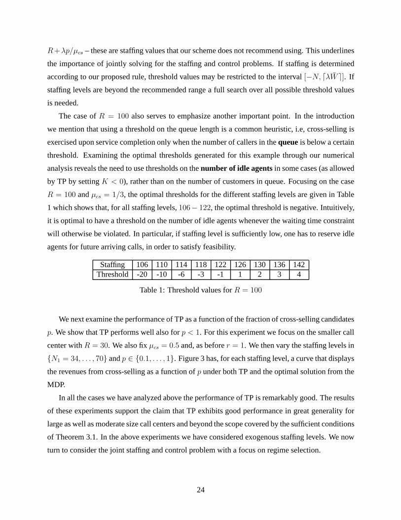
We next examine the performance of TP as a function of the fraction of cross-selling candidates
p. We show that TP performs well also forp < 1. For this experiment we focus on the smaller call
center withR = 30. We also fixµcs = 0.5 and, as beforer = 1. We then vary the staffing levels in
{N1 = 34, . . . , 70} andp ∈ {0.1, . . . , 1}. Figure 3 has, for each staffing level, a curve that displays
the revenues from cross-selling as a function ofp under both TP and the optimal solution from the
MDP.
In all the cases we have analyzed above the performance of TP is remarkably good. The results
of these experiments support the claim that TP exhibits goodperformance in great generality for
large as well as moderate size call centers and beyond the scope covered by the sufficient conditions
of Theorem 3.1. In the above experiments we have considered exogenous staffing levels. We now
turn to consider the joint staffing and control problem with afocus on regime selection.
24

ÓÔÕÖ×Ø ÓØ ÔØ ÕØ ÖÙ ÚÔ Ó
Ó Û Ø Ó Û Ô Ó Û Ü Ó Û Õ Ó Û Ý Ó Û Ö Ó Û Þ Ó Û × Ó Û ß Øà áâãã äå æççè éêë ìíæ
î
ï ð ñ ò ó ñ ô õ ö ÷ ð ó ò ø ï õ ù ò ú ö ÷ û ü ó ö ó ò ýþ ÿ� �� �� �� �� �� �� �� �� �
Figure 3: Performance of the TP rule as a function ofp (R = 30)
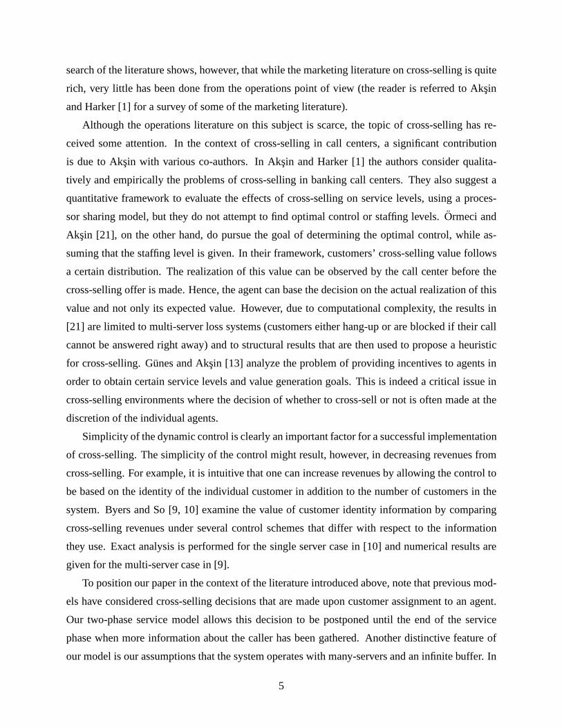
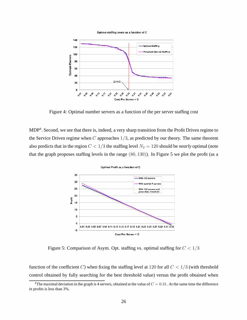
Staffing optimization and regime selection: We now provide a numerical example that illus-
trates the staffing selection procedure and relate it to the regime choice–Profit Driven vs. Service
Driven. Consider the settingR = 30, µs = 1 andµcs = 1/3, p = 1 andr = 1. We initially
assume that the cost function is linear, i.e, thatC(N) = C × N . In this case, the optimization
problem (21) has a simple solution (as a function of the cost coefficientC): If C ≥ rµcs = 1/3
thenN2 = R = 30. If C < rµcs, thenN2 = R + λp/µcs = 120. We calculateN1 as defined in
(11) to find thatN1 = 34. Hence, ifC < rµcs we haveN2 − R >> N1 − R and Theorem 3.1
asserts that the system is in the Profit Driven regime and thatthe asymptotically optimal staffing
level would beNλ2 . If C ≥ r/µcs, we expect the system to be operating in the Service Driven
regime. We now perform a numerical experiment to illustratethe strength of this regime character-
ization result. First, for each value ofC we find the optimal staffing by solving the MDP for each
staffing level and choosing the optimal one. The series that we obtain corresponds to the solid-line
series in Figure 4. In addition, for each value ofC we find the optimal staffing and threshold levels
assuming a threshold policy, and performing a full search tofind the best threshold value and the
corresponding optimal staffing level. The results are depicted in the dashed line in Figure 4. The
vertical line represents the critical valueC = 1/3.
We make the following two observations with respect to Figure 4. First, it shows that the TP
based staffing works extremely well for various cost figures.In particular, the staffing that we
obtain by using TP and a search for staffing is close to the optimal one that we obtain from the
25
� � �� �� � � � � �� ��� ����� ������
� � � � � ! " ! # ! $ �
% & � ' ( ) * � � ) + + ' , - * # * � ) � ) + . , / � ' � , � + �0 1 2 3 4 5 6 7 2 5 8 8 3 9 :; < = > ? < @ 6 A 0 1 2 3 4 5 6 7 2 5 8 8 3 9 :� $ B C
Figure 4: Optimal number servers as a function of the per server staffing cost
MDP4. Second, we see that there is, indeed, a very sharp transition from the Profit Driven regime to
the Service Driven regime whenC approaches1/3, as predicted by our theory. The same theorem
also predicts that in the regionC < 1/3 the staffing levelN2 = 120 should benearlyoptimal (note
that the graph proposes staffing levels in the range(80, 130)). In Figure 5 we plot the profit (as a
D EFEG FG EH FH EI FI EJ K J L J K J M J K J N J K J O J K J P J K L L J K L M J K L N J K L O J K L P J K Q L J K Q M J K Q N J K Q O J K Q P J K M L J K M MR STU VW
X Y Z [ \ ] ^ _ ] ^ ` ] ^ a X
b c [ d e f g \ ^ Y h d [ f Z f h i j k [ d Y j Y h X l m n o p q r s t u v t u sl m n o w x n m y z { | s t u v t u sl m n o p q r s t u v t u s z } ~x u t s � u m � t ~ n o u t s o w { ~Figure 5: Comparison of Asym. Opt. staffing vs. optimal staffing forC < 1/3
function of the coefficientC) when fixing the staffing level at120 for all C < 1/3 (with threshold
control obtained by fully searching for the best threshold value) versus the profit obtained when
4The maximal deviation in the graph is 4 servers, obtained at the value ofC = 0.31. At the same time the differencein profits is less than 3%.
26
using the optimal staffing level for each value ofC (with control as determined by the MDP). As
can be seen, these profits are close, so that using 120 servers, as proposed by our scheme for the
PD regime, results in a nearly optimal solution. Moreover, even if one does not search for the best
threshold value, but uses an arbitrary value ofK ∈ [0, dλWe], the performance with 120 servers
is still close to optimal. This can be seen as the dotted line that corresponds to the expected profit
when using 120 servers and a fixed thresholdK = 2 < λW = 3.
We now provide a numerical illustration of this point using the setting withR = 30 andµcs =
1/3. We assume a piecewise linear cost function with 3 break points. Specifically, we assume that
C(x) =
c1 × x x ≤ 40,c1 × 40 + c2 × (x − 40) 40 ≤ x ≤ 60c1 × 40 + c2 × 20 + c3 × (x − 60) 60 ≤ x ≤ 80c1 × 40 + c2 × 20 + c3 × 20 + c3 × (x − 80) x ≥ 80
The convexity is imposed by assuming thatc1 ≤ c2 ≤ c3 ≤ c4.
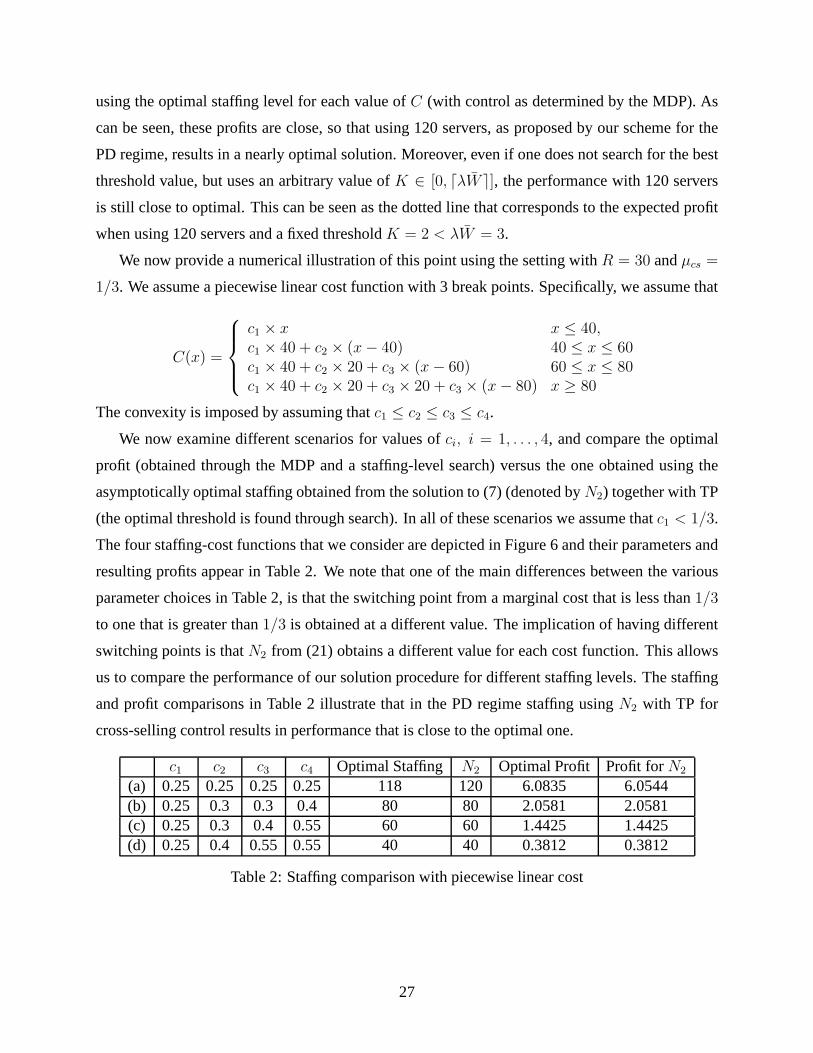
We now examine different scenarios for values ofci, i = 1, . . . , 4, and compare the optimal
profit (obtained through the MDP and a staffing-level search)versus the one obtained using the
asymptotically optimal staffing obtained from the solutionto (7) (denoted byN2) together with TP
(the optimal threshold is found through search). In all of these scenarios we assume thatc1 < 1/3.
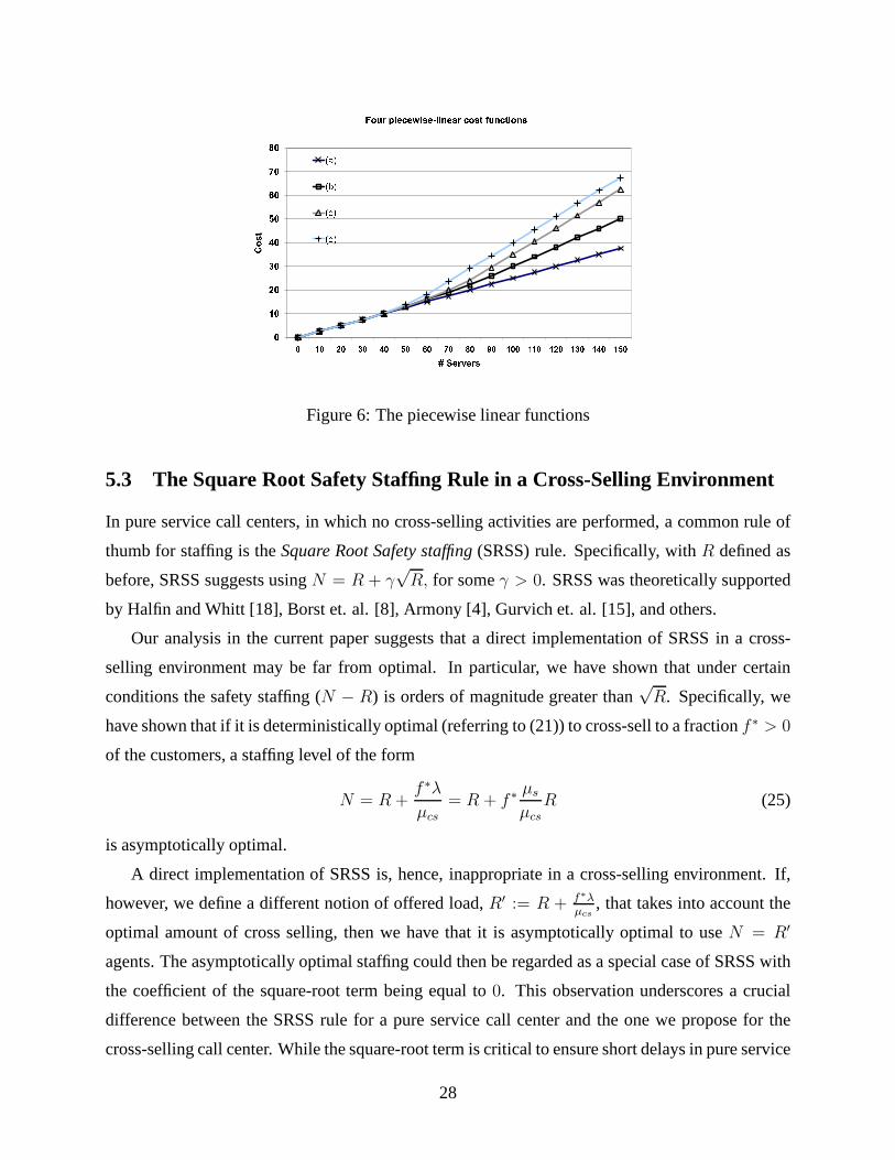
The four staffing-cost functions that we consider are depicted in Figure 6 and their parameters and
resulting profits appear in Table 2. We note that one of the main differences between the various
parameter choices in Table 2, is that the switching point from a marginal cost that is less than1/3
to one that is greater than1/3 is obtained at a different value. The implication of having different
switching points is thatN2 from (21) obtains a different value for each cost function. This allows
us to compare the performance of our solution procedure for different staffing levels. The staffing
and profit comparisons in Table 2 illustrate that in the PD regime staffing usingN2 with TP for
cross-selling control results in performance that is closeto the optimal one.
c1 c2 c3 c4 Optimal Staffing N2 Optimal Profit Profit forN2
(a) 0.25 0.25 0.25 0.25 118 120 6.0835 6.0544(b) 0.25 0.3 0.3 0.4 80 80 2.0581 2.0581(c) 0.25 0.3 0.4 0.55 60 60 1.4425 1.4425(d) 0.25 0.4 0.55 0.55 40 40 0.3812 0.3812
Table 2: Staffing comparison with piecewise linear cost
27
�� �� �� �� �� �� �� �� �� � � � � � � � � � � � � � � � � � � � � � � � � � � � � � � � � � � � �
� ���� � � � � � � �
� � � ¡ ¢ � £ � ¤ ¢ � � ¥ ¦ ¢ § � ¨ � £ � � © ª § £ © ¢ � § �« ¬ « ® « ¯ « ° Figure 6: The piecewise linear functions
5.3 The Square Root Safety Staffing Rule in a Cross-Selling Environment
In pure service call centers, in which no cross-selling activities are performed, a common rule of
thumb for staffing is theSquare Root Safety staffing(SRSS) rule. Specifically, withR defined as
before, SRSS suggests usingN = R + γ√
R, for someγ > 0. SRSS was theoretically supported
by Halfin and Whitt [18], Borst et. al. [8], Armony [4], Gurvich et. al. [15], and others.
Our analysis in the current paper suggests that a direct implementation of SRSS in a cross-
selling environment may be far from optimal. In particular,we have shown that under certain
conditions the safety staffing (N − R) is orders of magnitude greater than√
R. Specifically, we
have shown that if it is deterministically optimal (referring to (21)) to cross-sell to a fractionf ∗ > 0
of the customers, a staffing level of the form
N = R +f ∗λ
µcs= R + f ∗ µs
µcsR (25)
is asymptotically optimal.
A direct implementation of SRSS is, hence, inappropriate ina cross-selling environment. If,
however, we define a different notion of offered load,R′ := R + f∗λµcs
, that takes into account the
optimal amount of cross selling, then we have that it is asymptotically optimal to useN = R′
agents. The asymptotically optimal staffing could then be regarded as a special case of SRSS with
the coefficient of the square-root term being equal to0. This observation underscores a crucial
difference between the SRSS rule for a pure service call center and the one we propose for the
cross-selling call center. While the square-root term is critical to ensure short delays in pure service
28
systems, it would be of little importance in cross-selling systems where the capacity dedicated
to cross-selling is significant, i.e, in the profit driven regime. In particular, in the cross-selling
system one may ignore the square root component, since the service level is easily guaranteed
by fine tuning the amount of cross-selling (and the waiting time) by adjusting the threshold level
associated with the TP control.
How do these simple observations relate to call center practice? In practice, call center man-
agers might regard the observed handling times as consisting of a single phase and ignore the fact
that the observed handling times are not only often composedof two phases but are actually highly
dependent on the cross-selling control used. In particular, higher handling times will be observed
when the control leads to increased cross-selling. Basing the staffing decision on a naive estimate
of the handling times might then lead to inappropriate staffing levels. Interestingly, if a call center
is already cross-selling to its optimal fractionf ∗, its naive estimate of the mean handling time will
be 1µs
+ f∗
µcs. In particular, the estimate of the offered load will beR′ = λ
µs+ λf∗
µcs, so that using
SRSS will most likely perform rather well under a reasonablecontrol rule. If, on the other hand,
the call-center starts by operating away from its optimal fraction of cross-sold customers, this frac-
tion will remain sub-optimal regardless of the control used. Indeed, assume that the call center
usesN = R′ + γ√
R′ agents withR′ now equal toR + fλ/µcs for somef 6= f ∗. Then, since an
appropriately chosen square-root term is sufficient to guarantee service level satisfaction, the call
center will - under any reasonable policy (and in particularunder TP) - cross-sell very close to its
maximum capability which is given byµcs(N −R) = λf + O(√
R′). The new estimate of the av-
erage service time (which is obtained by averaging over all customers) will then be1µs
+ fµcs
+o(1).
Consequently, the call center will continue to perform sub-optimally. Observe that while theo(1)
component in the service time might have some effect on staffing, its cumulative effect will only
become significant in the very long-run.
6. Conclusions and Future Research
The practice of cross-selling in call centers is becoming prevalent and many organizations recog-
nize its revenue potential. Yet, operational aspects of cross-selling have so far attracted little at-
tention in the literature. In particular, very few papers address the control problem of determining
when to exercise cross-selling opportunities, and (to the best of our knowledge) this work (together
with [14]) is the first to address the staffing problem of determining how many customer service
representatives are needed. Those papers that have dealt with the control problem all illustrate that
29
solving this problem is difficult, which could indeed be the reason why no simple solutions have
been proposed so far. In this paper we have tackled the joint problem of determining staffing and
control by using an asymptotic approach, in which we look fora staffing level and a control which
might not be optimal for each particular problem instance, but they areasymptoticallyoptimal in
the sense that they perform extremely well, in the limit, as the arrival rate grows large.
Our approach has allowed us to not only refine the commonly used Threshold Priority (TP)
control rule, but to also propose a corresponding staffing rule. Under a set of assumptions on
system parameters, the staffing and control rules are asymptotically optimal in the limit as the
system size grows large. We have also shown numerically, that they perform well in various
settings for systems with relatively small arrival rate.
A naive approach would be to determine the staffing level ignoring the existence of cross-
selling, taking into account only staffing costs, service level constraints and service time. This
approach can lead to far from optimal solutions. To properlymanage cross-selling, one should take
into account the value of cross-selling and the associated additional handling time when making
staffing and control decisions. The simple structure of our solution allows managers to easily
incorporate this data in addition to pre-specified service-level targets into the staffing and control
decision.
This more comprehensive approach towards staffing and control of call centers with cross-
selling can prevent service-level degradation when transforming a pure-service call-center into one
that combines service and cross-selling activities. We have shown that call-centers with valuable
cross-selling have the capability to provide very short waiting times and, at the same time, obtain
revenues that are close to the optimal revenues obtained in the absence of waiting-time constraints.
Many questions remain unanswered with respect to the operational aspects of cross-selling in
call centers. Particularly, it is unclear how the customers’ experience prior to the cross-selling of-
fering affects their tendency to a) listen to the offer and b)purchase the product. Clearly, though,
if customers’ experience has a significant effect on these two tendencies, then one must take this
dependence into account when determining the staffing and control. Empirical and experimen-
tal research can be helpful in determining how callers actually respond to cross-selling offerings
depending on factors such as their delay, service time and overall quality of service. Another in-
teresting question is how to utilize the customer identity when determining whether to exercise a
cross-selling opportunity and what products to attempt to sell. A follow-up paper [14] addresses
some of these questions by studying the effect of customer heterogeneity on operational and eco-
nomic controls emphasizing the impact of the firm’s ability to customize its decisions based on
30
individual customer characteristics.
Table of Main Notationλ arrival rateµs service rateµcs cross-selling rateR = λ/µs offered loadN number of serversp fraction of callers who are cross-selling candidatesr expected revenue from cross-sellingπ control policyZ1 number of servers providing serviceZ2 number of servers performing cross-sellingZ = Z1 + Z2 total number of busy serversI = N − Z total number of idle serversQ queue lengthY = Z + Q total number of customers in the systemW virtual waiting timeW upper bound on the expected waitP{cs} long run proportion of customers that go through cross sellingC(·) staffing cost functionTP [K] threshold priority policy with threshold levelK
31
References
[1] Aksin O.Z., Harker P.T., “To sell or not to sell: Determining the trade-offs between serviceand sales in retail banking phone centers”.Journal of Service Research, 2(1), pp. 19-33, 1999.
[2] Altman E., “Constrained Markov Decision Processes”, Chapman & Hall/CRC, London,1999.
[3] Armony M., Mandelbaum A., “Routing and staffing in large-scaled service systems withheterogeneous servers and impatient customers”, Working Paper, NYU, New York, NY, 2006.
[4] Armony M., “Dynamic routing in large-scale service systems with heterogeneous servers”,Queueing Systems, 51(3-4), pp. 287-329, 2005.
[5] Armony M., Maglaras C., “On customer contact centers with a call-back option: customerdecisions, routing rules and system design”,Operations Research, 52(2), pp. 271-292, 2004.
[6] Armony M., Maglaras C., “Contact centers with a call-back option and real-time delay infor-mation”,Operations Research, 52(4), pp. 527-545, 2004.
[7] Aydin G. and Ziya S., “Pricing promotional products under upselling”, Manufacturing &Service Operations Management, 10, pp. 360-376, 2008.
[8] Borst S., Mandelbaum A. and Reiman M., “Dimensioning Large Call Centers”,OperationsResearch, 52(1), pp. 17-34, 2004.
[9] Byers R.E. and So K.C., “The value of information-based cross-sales policies in telephoneservice centers”, Working Paper, Graduate School of Management, University of California,Irvine, CA, 2004.
[10] Byers R.E. and So K.C., “A mathematical model for evaluating cross-sales policies in tele-phone service centers”,Manufacturing & Service Operations Management, 9(1), 1-8. 2007.
[11] Eichfeld A., Morse T.D. and Scott K.W., “Using call centers to boost revenue”, McKinseyQuarterly, May 2006.
[12] Gans N. and Zhou Y.-P., “A call-routing problem with service-level constraints”,OperationsResearch, 51(2), pp. 255-271, 2003.
[13] Gunes E.D. and Aksin O.Z., “Value creation in service delivery: Relating market segmenta-tion, incentives, and operational performance”,Manufacturing & Service Operations Man-agement, 6(4), pp. 338-357, 2004.
[14] Gurvich I., Armony M. and Maglaras C., “Cross-Selling in call centers with a heterogeneouspopulation”,Operations Research, forthcoming, 2008.
[15] Gurvich I., Armony M. and Mandelbaum A., “Service leveldifferentiation in call centerswith fully flexible servers”,Management Science, 54(2), pp. 279-294, 2008.
[16] Gurvich I. and Whitt W., “Scheduling flexible servers with convex delay costs in many-serverservice systems”,Manufacturing & Service Operations Management, forthcoming, 2008.
32
[17] Gurvich I. and Zeevi A., “Validity of heavy-traffic steady-state approximations in openqueueing networks: Sufficient conditions involving state-space collapse”, Working Paper,Columbia University, New York, NY, 2007.
[18] Halfin S. and Whitt W., “Heavy-traffic limits for queues with many exponential servers”,Operations Research, 29, pp. 567-587, 1981.
[19] Mandelbaum A. and Zeltyn S., “Staffing many-server queues with impatient customers: con-straint satisfaction in call centers”, Working Paper, Technion - Israel Institute of Technology,Haifa, Israel 2007.
[20] Netessine S., Savin S. and Xiao W., “Dynamic revenue management through cross-selling inE-commerce retailing”,Operations Research, 54(5), pp. 893-913, 2006.
[21] Ormeci E.L. and Aksin O.Z., “Revenue management through dynamic cross-selling in callcenters”, Working Paper, Koc University, Istanbul, Turkey, 2006.
[22] Puterman, M.L., “Markov decision processes: Discretestochastic dynamic programming”,Wiley, New York, NY, 1994.
[23] Wolff R.W., “Stochastic Modeling and the Theory of Queues”, Prentice Hall, EnglewoodCliffs, NJ, 1989.
33