Where does the carbon go? A modeldata …Where does the carbon go? A model–data intercomparison of vegetation carbon allocation and turnover processes at two temperate forest free-air

Where does the carbon go? A model–data intercomparison ofvegetation carbon allocation and turnover processes at twotemperate forest free-air CO2 enrichment sites

Martin G. De Kauwe1, Belinda E. Medlyn1, S€onke Zaehle2, Anthony P. Walker3, Michael C. Dietze4, Ying-Ping

Wang5, Yiqi Luo6, Atul K. Jain7, Bassil El-Masri7, Thomas Hickler8,9, David W�arlind10, Ensheng Weng11, William

J. Parton12, Peter E. Thornton3, Shusen Wang13, I. Colin Prentice1,14, Shinichi Asao12, Benjamin Smith10, Heather

R. McCarthy15, Colleen M. Iversen3, Paul J. Hanson3, Jeffrey M. Warren3, Ram Oren16,17 and Richard J. Norby3

1Department of Biological Sciences, Macquarie University, Sydney, New South Wales 2109, Australia; 2Biogeochemical Integration Department, Max Planck Institute for Biogeochemistry,

Hans-Kn€oll-Str. 10, 07745 Jena, Germany; 3Environmental Sciences Division and Climate Change Science Institute, Oak Ridge National Laboratory, Oak Ridge, TN 37831-6301, USA;

4Department of Earth and Environment, Boston University, Boston, MA 02215, USA; 5CSIRO Marine and Atmospheric Research and Centre for Australian Weather and Climate Research,

Private Bag #1, Aspendale, Victoria 3195, Australia; 6Department of Microbiology and Plant Biology, University of Oklahoma, Norman, OK 73019, USA; 7Department of Atmospheric

Sciences, University of Illinois, 105 South Gregory Street, Urbana, IL 61801, USA; 8Biodiversity and Climate Research Centre (BiK-F) & Senckenberg Gesellschaft f€ur Naturforschung,

Senckenberganlage 25, 60325 Frankfurt/Main, Germany; 9Department of Physical Geography, Goethe-University, Altenh€oferalle 1, 60438 Frankfurt/Main, Germany; 10Department of

Physical Geography and Ecosystem Science, Lund University, Lund, Sweden; 11Department of Ecology and Evolutionary Biology, Princeton University, Princeton, NJ 08544, USA; 12Natural

Resource Ecology Laboratory, Colorado State University, Fort Collins, CO 80523-1499, USA; 13Canada Centre for Remote Sensing, Natural Resources Canada, Ottawa, Canada; 14AXA Chair

of Biosphere and Climate Impacts, Department of Life Sciences, Grand Challenges in Ecosystems and the Environment and Grantham Institute for Climate Change, Imperial College London,

London, UK; 15Department of Microbiology and Plant Biology, University of Oklahoma, 770 Van Vleet Oval, Norman, OK 73019, USA; 16Division of Environmental Science & Policy,

Nicholas School of the Environment, Duke University, Durham, NC 27708, USA; 17Department of Forest Ecology & Management, Swedish University of Agricultural Sciences (SLU), SE-901

83, Umea, Sweden

Author for correspondence:Martin G. De Kauwe

Tel: +61 2 9850 9256Email: [email protected]

Received: 21 January 2014

Accepted: 8 April 2014

New Phytologist (2014) 203: 883–899doi: 10.1111/nph.12847

Key words: allocation, carbon (C), climatechange, CO2 fertilisation, elevated CO2,free-air CO2 enrichment (FACE), models,phenology.

Summary

� Elevated atmospheric CO2 concentration (eCO2) has the potential to increase vegetation

carbon storage if increased net primary production causes increased long-lived biomass.

Model predictions of eCO2 effects on vegetation carbon storage depend on how allocation

and turnover processes are represented.� We used data from two temperate forest free-air CO2 enrichment (FACE) experiments to

evaluate representations of allocation and turnover in 11 ecosystem models.� Observed eCO2 effects on allocation were dynamic. Allocation schemes based on func-

tional relationships among biomass fractions that vary with resource availability were best able

to capture the general features of the observations. Allocation schemes based on constant

fractions or resource limitations performed less well, with some models having unintended

outcomes. Few models represent turnover processes mechanistically and there was wide vari-

ation in predictions of tissue lifespan. Consequently, models did not perform well at predicting

eCO2 effects on vegetation carbon storage.� Our recommendations to reduce uncertainty include: use of allocation schemes constrained

by biomass fractions; careful testing of allocation schemes; and synthesis of allocation and

turnover data in terms of model parameters. Data from intensively studied ecosystem manip-

ulation experiments are invaluable for constraining models and we recommend that such

experiments should attempt to fully quantify carbon, water and nutrient budgets.

Introduction

Since the industrial revolution, burning fossil fuels and land-usechange have driven an increase of c. 44% in the atmospheric con-centration of carbon dioxide ([CO2]) (Le Qu�er�e et al., 2013).Current projections from coupled climate–carbon models suggest

that the concentration may reach anywhere between c. 490 and1370 ppm by 2100 (Moss et al., 2010). Elevated [CO2] (eCO2)stimulates plant photosynthesis, which has the potential toincrease net primary productivity (NPP) of vegetation (Kimball,1983; Norby et al., 2005). Many studies have investigated thisNPP response, both experimentally using large-scale CO2

� 2014 The Authors

New Phytologist� 2014 New Phytologist TrustNew Phytologist (2014) 203: 883–899 883

www.newphytologist.comThis is an open access article under the terms of the Creative Commons Attribution License, which permits use,distribution and reproduction in any medium, provided the original work is properly cited.

Research

enrichment facilities, and also with ecosystem models (Orenet al., 2001; Luo et al., 2004; McCarthy et al., 2010; Norby et al.,2010; Drake et al., 2011; Reich & Hobbie, 2012; Zaehle et al.,2014).

Ultimately, however, the effect of eCO2 on NPP by itself isnot as important as its consequences for key ecosystem properties,such as leaf area index (LAI) and vegetation carbon (C) storage.LAI is an important ecosystem property, with consequences forsurface temperature and water balance. Vegetation C storage is amajor component of the C cycle; c. 360 Pg C, or c. 20% of allterrestrial C, is stored in live forest biomass (Bonan, 2008; Panet al., 2011). Rising NPP due to CO2 fertilisation may lead toincreased biomass C storage, which creates a strong negative feed-back on rising atmospheric [CO2] (Canadell et al., 2007; LeQu�er�e et al., 2009). Increased NPP can also lead to increasedinput of plant detritus into the soil system, potentially increasingC storage in long-lived soil pools (Iversen et al., 2012).

In order to predict changes in these ecosystem properties, weneed to understand not only how eCO2 affects NPP, but alsohow it affects the allocation of the assimilated C to plant tissues.The effects of eCO2 on plant C storage will differ considerably ifthe C is allocated towards long-lived plant tissue (i.e. woodycomponents), where it remains sequestered over long time peri-ods; or alternatively, if cycling of C through the system isincreased via increased allocation to short-lived tissues or reducedtissue lifespan (Luo et al., 2003; Korner et al., 2005). Similarly,the effects of eCO2 on LAI depend on changes in NPP but alsoon changes in the fraction of C allocated to foliage vs other plantcomponents.

Currently, global vegetation models predict that eCO2 willlead to increasing C sequestration in both the biomass and soil(Cox et al., 2000; Cramer et al., 2001; Friedlingstein et al., 2006;Lenton et al., 2006; Schaphoff et al., 2006; Thornton et al.,2007; Arora et al., 2013), but the simulated C-store (live biomassand soils) diverges considerably between simulations. Jones et al.(2013) showed a large spread in the simulated change in the landC-store of between c. �250 and 400 Pg C by 2100 from a seriesof model simulations run as part of the Coupled Model Inter-comparison Project (CMIP5). There are many possible causes forthis among-model variability, but one important differenceamong models is the representation of C allocation and poolturnover patterns. The choice of model allocation scheme hasbeen shown to have significant consequences for predicted bio-mass responses. For example, Friedlingstein et al. (1999) showedthat the CASA model would predict a 10% reduction in globalbiomass by replacing fixed empirical constants with a dynamic Callocation scheme based on resource availability (light, water andnitrogen (N)). Similarly, Ise et al. (2010) found large variability(up to 29%) among model estimates of woody biomass causedby different assumptions about C allocation coefficients. Weng& Luo (2011) evaluated the TECO model at the Duke site andfound that partitioning to woody biomass to be the most sensi-tive parameter governing predictions of ecosystem carbon stor-age. Most recently, Friend et al. (2014) attributed uncertainty inmulti-model predictions of the future vegetation store to differ-ent residence times in models.

In order to understand why models differ in their predictionsof C sequestration, and to reduce this uncertainty, we need toidentify the assumptions made in different models and examinehow these assumptions impact on model predictions. Experimen-tal data can then be used to help distinguish the best modelassumptions. We applied a series of 11 ecosystem models to datafrom two temperate forest free-air CO2 enrichment (FACE) sites.In previous papers we used this assumption-centred modellingapproach to examine model assumptions related to NPP andwater use (De Kauwe et al., 2013; Zaehle et al., 2014; Walkeret al., 2014) . In this paper, we focus on the processes of alloca-tion and turnover. We document how each of the 11 models rep-resent these processes. We then quantify how these processrepresentations affect predictions of vegetation C storage andLAI, and compare the models against measurements at the twosites in order to understand which process representations havethe capacity to capture observed responses.

In the absence of a mechanistic understanding of the processescontrolling C allocation at the whole-plant level, models eitherfollow empirical or evolutionary-based approaches (Franklinet al., 2012). Empirical approaches include fixed coefficients, al-lometric scaling or functional balance approaches, while evolu-tionary-based approaches include optimisation, game-theoreticapproaches and adaptive dynamics (Dybzinski et al., 2011;Franklin et al., 2012; Farrior et al., 2013). The set of models usedin this model intercomparison employed all of these approaches,with the exception of game theory and adaptive dynamics, whichhave not yet been widely employed in ecosystem models. Wewere therefore able to probe differences in the predicted CO2

responses of allocation processes among the most commonlyemployed model approaches.

Materials and Methods

Terminology

The terminology used to describe C allocation processes withinthe literature is rather ambiguous. Litton et al. (2007) proposed aseries of definitions to standardise usage in experimental studies.Unfortunately, these definitions do not correspond directly to theway that processes are represented within most ecosystem models,which typically consider C allocation in terms of available NPPrather than Gross Primary Production (GPP). In this paper,therefore, we use terms that are defined according to typical eco-system model structure. Many ecosystem models are basedaround differential equations for biomass, which can be mostsimply expressed as:

dBi=dt ¼ aiNPP� uiBi Eqn 1

(i, ith plant component; Bi, biomass of that component (kg m�2);ai, fractions summing to 1; ui, turnover rates of each component(yr�1)). We considered the plant components to be foliage, wood(including stem, branch and coarse roots), fine roots and repro-duction. We defined ‘allocation coefficients’ to mean the fractions

New Phytologist (2014) 203: 883–899 � 2014 The Authors

New Phytologist� 2014 New Phytologist Trustwww.newphytologist.com

Research

NewPhytologist884

ai that determine the division of NPP among the plant compo-nents. We also defined ‘biomass fractions’ to mean the fraction oftotal plant biomass present in each component at a given time. Ascan be seen from Eqn (1), the biomass fractions depend both onthe allocation coefficients and turnover rates.

Experimental data

Models were applied to two experimental sites, both of whichhave been extensively described elsewhere (Norby et al., 2001;McCarthy et al., 2010; Walker et al., 2014). The Duke FACE sitewas situated in a loblolly pine (Pinus taeda) plantation in NorthCarolina, USA (35.97°N, 79.08°W). The Duke experiment wasinitiated in 1996, when trees were 13 yr old. By the end of theexperiment (2007), there was a significant hardwood understoreyin addition to the overstorey pines. Data used in this paper referto the forest stand as a whole, thus including both pines andhardwoods, because fine root production data were not separatedby species. Six 30-m diameter plots were established, and CO2

treatments were initiated in August 1996. Three of these plotstracked ambient conditions and three plots received continuousenhanced CO2 concentrations of +200 lmol mol�1 (mean c.542 lmol mol�1).

The ORNL FACE site was located in Tennessee, USA, at theOak Ridge National Laboratory (35.9°N, 84.33°W) and is asweetgum (Liquidambar styraciflua) plantation, established in1988 on a former grassland. Treatment began at Oak Ridge in1998 with two elevated rings (c. 25 m diameter) with an averagegrowing season [CO2] of 547 lmol mol�1 and three ambientCO2 (aCO2) rings (c. 395 lmol mol�1).

Detailed measurements were collected during the experimentsat both sites. Data used in this study included biomass, litterfalland NPP of each component (foliage, wood and fine root), andtotal leaf area index (LAI). NPP at both sites was calculated as thesum of woody biomass increment (estimated from allometricrelationships between biomass and tree diameter and height),foliage productions (from litter traps), and fine-root production(from minirhizotron observations), as fully described by Norbyet al. (2005) and references cited therein. At Duke FACE, obser-vations of growth and litter components were only available from1996 to 2005, whereas at ORNL FACE observations were avail-able from 1998 to 2008. In this study we analysed model resultsfor the corresponding periods for which we had observations, thatis, 1996–2005 at Duke and 1998–2008 at Oak Ridge. Thesedata are described in detail elsewhere, for Duke in McCarthyet al. (2007, 2010) and for Oak Ridge in Norby et al. (2001,2004), and Iversen et al. (2008). These datasets are available at:http://public.ornl.gov/face/index.shtml.

From these data we calculated annual allocation coefficientsfor the foliage, wood, fine roots (growth of coarse roots wasincluded in the wood component) and reproduction over thewhole experiment. Allocation coefficients were calculated as NPPof individual components divided by total NPP. Turnover coeffi-cients were calculated on an annual basis as the annual sum oflitter divided by the annual maximum of each biomass compo-nent (foliage, wood and fine roots). The lifespan of each

component is defined as the inverse of the turnover coefficients.In addition, we calculated whole-canopy specific leaf area as LAIdivided by foliage biomass.

Model simulations

The 11 models applied to the two FACE sites include stand(GDAY, CENTURY, TECO), age/size-gap (ED2, LPJ-GUESS),land surface (CABLE, CLM4, EALCO, ISAM, O-CN) anddynamic vegetation models (SDGVM). A detailed overview ofthe models is given in Walker et al. (2014), and detailed analysesof the water and N cycle responses are provided by De Kauweet al. (2013) and Zaehle et al. (2014) respectively.

Each model was used to run simulations covering 1996–2008at the Duke FACE site and 1998–2009 at the ORNL FACE site.Modellers were provided with general site characteristics, meteo-rological forcing and CO2 concentration data. Most models sim-ulated the Duke FACE site as a coniferous evergreen canopy,although ED2 and LPJ-GUESS included a hardwood fraction.All models simulated the ORNL FACE site as a broadleaf decid-uous canopy (Walker et al., 2014). Models output a variety of C,N and water fluxes at their appropriate driving resolution (hourlyor daily).

Analysis approach

We deliberately did not statistically evaluate any of the modelsagainst observations, because models can easily yield quantita-tively good responses for incorrect reasons; thus such an approachtypically does not correctly diagnose model deficiencies (Medlynet al., 2005; Abramowitz et al., 2008; Walker et al., 2014). Fur-thermore, at both sites a series of storm events introduced tran-sient system responses which are not accounted for in the models,complicating direct point comparisons. Instead, we assessed themodel performance qualitatively by attempting to understand thepredictions made based on the underlying assumptions relatingto allocation and turnover processes. In assessing model perfor-mance, a ‘good’ model is one that captures the processes underly-ing response of the system to eCO2, although it may notexplicitly match the temporal dynamics observed at individualsites.

We first documented how the allocation process is representedin each of the 11 models. For some models, the sum of annualplant growth does not exactly equal total photosynthesis less res-piration in each year, due to the presence of a nonstructural labilecarbon pool. The modelled size of this pool varies among modelsdepending on how transfer from storage to growth is represented,but within a model remains relatively constant over the course ofthe experiment (see Supporting Information Notes S1, Fig. S1a,b). Because there are no estimates of this pool size for eitherexperiment, we could not evaluate the modelled labile C poolagainst data. In what follows, therefore, we focus on the alloca-tion of carbon used for growth among different plant tissues. Wecalculated the allocation coefficients ai from model outputs ofannual growth of each plant component, and compared the mod-elled allocation coefficients at aCO2 and elevated CO2 (eCO2) at


New Phytologist� 2014 New Phytologist TrustNew Phytologist (2014) 203: 883–899

www.newphytologist.com

NewPhytologist Research 885

the two sites against the observed values. The results for the allo-cation coefficients were interpreted in terms of the underlyingmodel representation of allocation.

We then examined the models’ predicted CO2 responses ofleaf area index (LAI, representing canopy cover) and C sequestra-tion in woody biomass. Predicted LAI depends on specific leafarea (SLA), the ratio of leaf area to leaf mass, as well as allocationcoefficients. Therefore, we also documented how the models rep-resented SLA. Similarly, predicted C sequestration also dependson tissue turnover, so we documented how the models repre-sented turnover. Finally, we analysed how the representations ofthese processes combined to determine the model predictions.

Model representations of allocation

We classified the ways that C allocation is implemented in themodels into four general classes: (1) fixed coefficients; (2) func-tional relationships; (3) resource limitations; and (4) optimisa-tion. In fixed-coefficient models, a fixed fraction of NPP isallocated to each plant component. In functional-relationshipmodels, relationships among plant organs provide constraintsfrom which the allocation coefficients can be determined. In gen-eral, these relationships are based on the hypotheses that (1) sap-wood cross-sectional area must be sufficient to supply structuralsupport and water transport for the leaf area (the pipe-modelhypothesis, Shinozaki et al., 1964a,b) and (2) root activity andleaf activity should be balanced (the functional balance hypothe-sis, Davidson, 1969). In resource-limitation models, the allocationcoefficients are adjusted according to which resource is most lim-iting to growth. Resource-limitation models are based on similarideas to the functional relationship models, but the key distinc-tion is that relationships are calculated among allocation coeffi-cients rather than among the biomass fractions. In optimisationmodels, allocation coefficients are varied to maximise some mea-sure of performance by the plants.

Each of the 11 ecosystem models was classified into one ofthese four groups. Classifications and a full description of howeach model represents allocation are given in Table 1. Manymodels separately consider allocation to bole, branches and coarseroots, whereas others lump these components into wood. Here,we consider only the combined component wood to enable com-parison among models. Three models, ED2, LPJ-GUESS andO-CN, also utilise a proportion of available C for reproduction.

Results

Allocation patterns

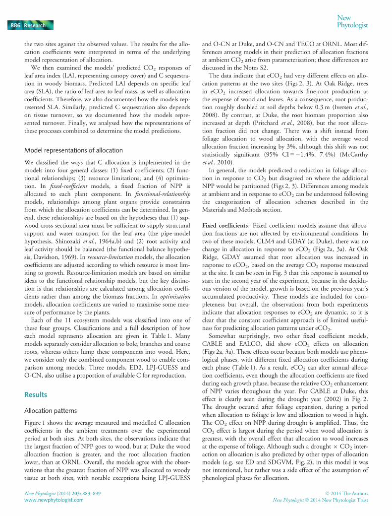
Figure 1 shows the average measured and modelled C allocationcoefficients in the ambient treatments over the experimentalperiod at both sites. At both sites, the observations indicate thatthe largest fraction of NPP goes to wood, but at Duke the woodallocation fraction is greater, and the root allocation fractionlower, than at ORNL. Overall, the models agree with the obser-vations that the greatest fraction of NPP was allocated to woodytissue at both sites, with notable exceptions being LPJ-GUESS

and O-CN at Duke, and O-CN and TECO at ORNL. Most dif-ferences among models in their prediction of allocation fractionsat ambient CO2 arise from parameterisation; these differences arediscussed in the Notes S2.

The data indicate that eCO2 had very different effects on allo-cation patterns at the two sites (Figs 2, 3). At Oak Ridge, treesin eCO2 increased allocation towards fine-root production atthe expense of wood and leaves. As a consequence, root produc-tion roughly doubled at soil depths below 0.3 m (Iversen et al.,2008). By contrast, at Duke, the root biomass proportion alsoincreased at depth (Pritchard et al., 2008), but the root alloca-tion fraction did not change. There was a shift instead fromfoliage allocation to wood allocation, with the average woodallocation fraction increasing by 3%, although this shift was notstatistically significant (95% CI =�1.4%, 7.4%) (McCarthyet al., 2010).

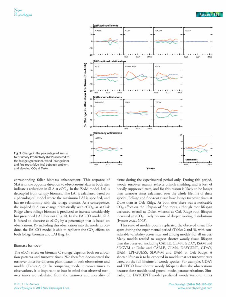
In general, the models predicted a reduction in foliage alloca-tion in response to CO2 but disagreed on where the additionalNPP would be partitioned (Figs 2, 3). Differences among modelsat ambient and in response to eCO2 can be understood followingthe categorisation of allocation schemes described in theMaterials and Methods section.

Fixed coefficients Fixed coefficient models assume that alloca-tion fractions are not affected by environmental conditions. Intwo of these models, CLM4 and GDAY (at Duke), there was nochange in allocation in response to eCO2 (Figs 2a, 3a). At OakRidge, GDAY assumed that root allocation was increased inresponse to eCO2, based on the average CO2 response measuredat the site. It can be seen in Fig. 3 that this response is assumed tostart in the second year of the experiment, because in the decidu-ous version of the model, growth is based on the previous year’saccumulated productivity. These models are included for com-pleteness but overall, the observations from both experimentsindicate that allocation responses to eCO2 are dynamic, so it isclear that the constant coefficient approach is of limited useful-ness for predicting allocation patterns under eCO2.

Somewhat surprisingly, two other fixed coefficient models,CABLE and EALCO, did show eCO2 effects on allocation(Figs 2a, 3a). These effects occur because both models use pheno-logical phases, with different fixed allocation coefficients duringeach phase (Table 1). As a result, eCO2 can alter annual alloca-tion coefficients, even though the allocation coefficients are fixedduring each growth phase, because the relative CO2 enhancementof NPP varies throughout the year. For CABLE at Duke, thiseffect is clearly seen during the drought year (2002) in Fig. 2.The drought occured after foliage expansion, during a periodwhen allocation to foliage is low and allocation to wood is high.The CO2 effect on NPP during drought is amplified. Thus, theCO2 effect is largest during the period when wood allocation isgreatest, with the overall effect that allocation to wood increasesat the expense of foliage. Although such a drought 9 CO2 inter-action on allocation is also predicted by other types of allocationmodels (e.g. see ED and SDGVM, Fig. 2), in this model it wasnot intentional, but rather was a side effect of the assumption ofphenological phases for allocation.



Research

NewPhytologist886

In EALCO, the assumption that the period of foliage alloca-tion continues until the observed maximum LAI is reachedimplies that annual foliage allocation is determined by theobserved LAI. The fine-root allocation coefficient is fixed, andwood allocation is therefore the remainder of NPP. At Duke,where observed root allocation was not affected by eCO2, theallocation patterns simulated by EALCO resemble the observa-tions (Fig. 2). At Oak Ridge, by contrast, where observed rootallocation was strongly affected by eCO2, the allocation patternssimulated by EALCO differ strongly from the observations(Fig. 3). As with CABLE, however, these eCO2 effects were anunintended consequence of the phenology of the allocationscheme.

Functional relationships The three models ED2, LPJ-GUESSand O-CN allocate C according to functional relationshipsamong plant organs, which maintain sapwood, foliage and fineroots in ratios that vary according to N and water availability.The allocation responses to CO2 predicted by these three modelsare relatively consistent (Figs 2b, 3b), and capture the observedresponses to some extent. With the additional increase in produc-tivity in response to CO2, all three models predict that initiallywood allocation must increase to supply the extra wood volumenecessary to maintain the same leaf to sapwood area ratio. InED2, this effect continues throughout the experiment, becausehigh available soil N means that nutrient limitation does notdevelop (Zaehle et al., 2014). In LPJ-GUESS and O-CN, water

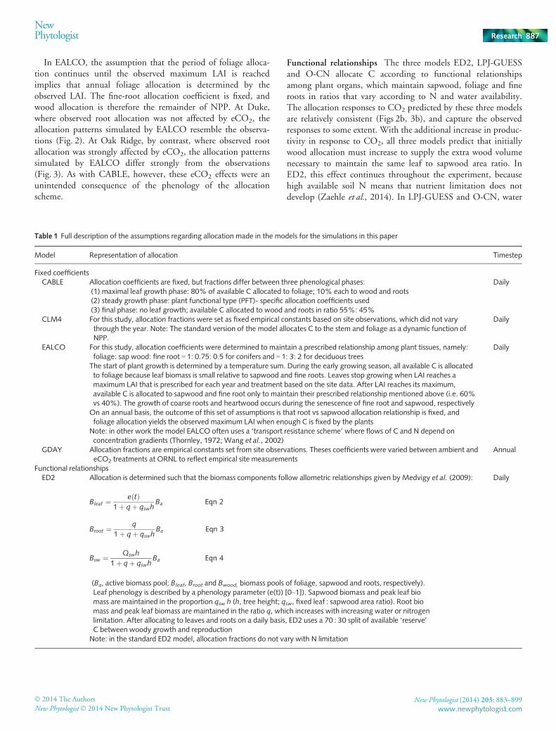
Table 1 Full description of the assumptions regarding allocation made in the models for the simulations in this paper

Model Representation of allocation Timestep

Fixed coefficientsCABLE Allocation coefficients are fixed, but fractions differ between three phenological phases:

(1) maximal leaf growth phase: 80% of available C allocated to foliage; 10% each to wood and roots(2) steady growth phase: plant functional type (PFT)- specific allocation coefficients used(3) final phase: no leaf growth; available C allocated to wood and roots in ratio 55%: 45%

Daily

CLM4 For this study, allocation fractions were set as fixed empirical constants based on site observations, which did not varythrough the year. Note: The standard version of the model allocates C to the stem and foliage as a dynamic function ofNPP.

Daily

EALCO For this study, allocation coefficients were determined to maintain a prescribed relationship among plant tissues, namely:foliage: sap wood: fine root = 1: 0.75: 0.5 for conifers and = 1: 3: 2 for deciduous treesThe start of plant growth is determined by a temperature sum. During the early growing season, all available C is allocatedto foliage because leaf biomass is small relative to sapwood and fine roots. Leaves stop growing when LAI reaches amaximum LAI that is prescribed for each year and treatment based on the site data. After LAI reaches its maximum,available C is allocated to sapwood and fine root only to maintain their prescribed relationship mentioned above (i.e. 60%vs 40%). The growth of coarse roots and heartwood occurs during the senescence of fine root and sapwood, respectivelyOn an annual basis, the outcome of this set of assumptions is that root vs sapwood allocation relationship is fixed, andfoliage allocation yields the observed maximum LAI when enough C is fixed by the plantsNote: in other work the model EALCO often uses a ‘transport resistance scheme’ where flows of C and N depend onconcentration gradients (Thornley, 1972; Wang et al., 2002)

Daily

GDAY Allocation fractions are empirical constants set from site observations. Theses coefficients were varied between ambient andeCO2 treatments at ORNL to reflect empirical site measurements

Annual

Functional relationshipsED2 Allocation is determined such that the biomass components follow allometric relationships given by Medvigy et al. (2009):

Bleaf ¼ eðtÞ1þ qþ qswh

Ba Eqn 2

Broot ¼ q

1þ qþ qswhBa Eqn 3

Bsw ¼ Qswh

1þ qþ qswhBa Eqn 4

(Ba, active biomass pool; Bleaf, Broot and Bwood, biomass pools of foliage, sapwood and roots, respectively).Leaf phenology is described by a phenology parameter (e(t)) [0–1]). Sapwood biomass and peak leaf biomass are maintained in the proportion qsw h (h, tree height; qsw, fixed leaf : sapwood area ratio). Root biomass and peak leaf biomass are maintained in the ratio q, which increases with increasing water or nitrogenlimitation. After allocating to leaves and roots on a daily basis, ED2 uses a 70 : 30 split of available ‘reserve’C between woody growth and reproductionNote: in the standard ED2 model, allocation fractions do not vary with N limitation

Daily





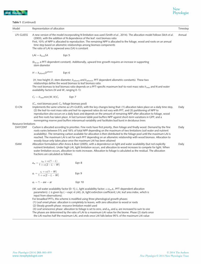
Table 1 (Continued)


LPJ-GUESS A new version of the model incorporating N limitation was used (Smith et al., 2014). The allocation model follows Sitch et al.

(2003), with the addition of N dependence of the leaf: root biomass ratioFirst, 10% of NPP is allocated to reproduction. The remaining NPP is allocated to the foliage, wood and roots on an annualtime step based on allometric relationships among biomass componentsThe ratio of LAI to sapwood area (SA) is constant

LAI ¼ kla:saSA Eqn 5

(kla:sa, a PFT-dependent constant). Additionally, upward tree growth requires an increase in supportingstem diameter

H ¼ kallom2Dallom3 Eqn 6

(H, tree height; D, stem diameter; kallom2 and kallom3, PFT dependent allometric constants). These tworelationships define the wood biomass to leaf biomass ratioThe root biomass to leaf biomass ratio depends on a PFT-specific maximum leaf-to-root mass ratio lrmax and N and wateravailability factors (N andW, ranging 0–1):

Cf ¼ lrmaxminðW;NÞCr Eqn 7

(Cr, root biomass pool; Cf, foliage biomass pool)

Annual

O-CN Implements the same scheme as LPJ-GUESS, with the key changes being that: (1) allocation takes place on a daily time step,(2) the leaf-to-root mass ratio and leaf-to-sapwood ratios do not vary with PFT, and (3) partitioning of NPP toreproduction also occurs on a daily basis and depends on the amount of remaining NPP after allocation to foliage, woodand fine roots has taken place. A fast turnover labile pool buffers NPP against short-term variations in GPP; and anonrespiring reserve pool buffers interannual variability and facilitates bud burst in deciduous trees

Daily

Resource limitationsDAYCENT Carbon is allocated according to priorities. Fine roots have first priority, then foliage and finally wood. Demand by the fine

roots varies between 5% and 18% of total NPP depending on the maximum of two limitations (soil water and nutrientavailability). The remaining carbon available for allocation is then distributed to the foliage pool until the maximum LAI isreached. The maximum LAI is set for each PFT depending on an allometric relationship with wood biomass. Allocation towoody tissue only takes place once the maximum LAI has been attained

Daily

ISAM Allocation formulation after Arora & Boer (2005), with a dependence on light and water availability (but not explicitlynutrient limitation). Under high LAI, light limitation occurs, and allocation to wood increases to compete for light. Whenwater limitation occurs, allocation to roots increases. Allocation to foliage is calculated as the residual. The allocationfractions are calculated as follows:

aw ¼ ew þ xð1� LÞ1þ xð2� L�WÞ Eqn 8

ar ¼ er þ xð1�WÞ1þ xð2� L�WÞ Eqn 9

af ¼ 1� aw� ar Eqn 10

(W, soil water availability factor [0–1]; L, light availability factor; x ɛw,ɛr, PFT-dependent allocationparameters). L is given by L = exp(–k LAI), (k, light extinction coefficient; LAI, leaf area index, which isinput from observations).For broadleaf PFTs, this scheme is modified using three phenological growth phases:(1) Leaf onset phase: allocation is completely to leaves, with zero allocation to wood or roots(2) Steady growth phase: resource limitation model used(3) Leaf senescence phase: allocation to foliage is set to zero, and aw and ar are increased to sum to oneThe phases are determined by the ratio of LAI to a maximum LAI value for the biome. Phase (2) starts oncethe LAI reaches half the maximum LAI, and ends once LAI falls below 95% of the maximum LAI value

Daily



Research

NewPhytologist888

and nutrient limitations develop over the course of the experi-ment, causing allocation to shift towards roots to maintain afunctional balance between foliage and roots. This effect is seenmost clearly in O-CN, in which increased N stress develops atboth sites. In LPJ-GUESS, the dynamics of allocation at OakRidge change following a simulated mortality event in 2005. Themortality reduces the stand-scale leaf:sapwood area ratio signifi-cantly, driving an increase in wood allocation in the last years ofthe experiment.

Resource limitations Three models, ISAM, DAYCENT andTECO use resource limitation approaches, in which allocationcoefficients are determined by limitations of water, light andnutrient availability. Although the approaches are similar in the-ory, the implementations are sufficiently different that the threemodels predict rather different allocation patterns and responsesto eCO2 (Figs 2, 3).

In ISAM, the allocation coefficients vary with water and lightlimitation (Table 1). However, the predicted CO2 effects on allo-cation differ between the sites because of the use of phenologicalphases in deciduous species. At Duke, eCO2 increased LAI,decreasing light availability, and reduced transpiration per unitleaf area, increasing water availability. Both effects cause anincrease in wood allocation (Fig. 2g), much like that predicted bythe allometric models, and somewhat similar to observations. Bycontrast, at Oak Ridge, foliage allocation is predicted to increasestrongly with eCO2 (Fig. 3g), as an unintentional side effect of

the use of phenological phases. The start of senescence period(the third phenological phase) occurs when the observed LAIdeclines to 95% of the prescribed maximum value. Because LAIis greater in the eCO2 treatment, the LAI does not fall below thesenescence threshold until considerably later than in the ambienttreatment (c. 20 d). As allocation to foliage continues until thesenescence phase starts, foliage allocation is increased consider-ably in response to CO2, in stark contrast to observations andother models.

The DAYCENT and TECO models use similar prioritisationschemes to decide allocation (Table 1). However, the predictedresponse of allocation to eCO2 differs between these two modelsbecause of different predicted impacts on water and nutrientstress. In DAYCENT, at Duke, root allocation was increasedwith eCO2 due to an increase in nutrient limitation. At OakRidge, by contrast, root allocation was unchanged, indicatingthat water and nutrient stress were unaffected by eCO2. At bothsites, foliage allocation decreased in response to eCO2 becausethe maximum prescribed LAI had been attained. As a result, allo-cation to wood (the third in the list of priorities) increased atOak Ridge, but not at Duke. These predictions differed markedlyfrom observations at both sites.

In the TECO model, at Duke, the maximum root allocationwas obtained at aCO2 and as result there was no CO2-inducedchange. At Oak Ridge, water stress was reduced under eCO2 as aconsequence of water savings due to stomatal closure, resulting inlower root allocation. At both sites, foliage allocation was reduced

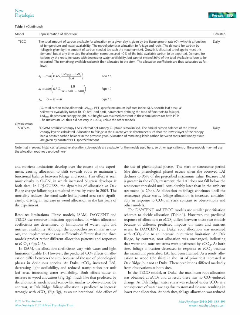
Table 1 (Continued)


TECO The total amount of carbon available for allocation on a given day is given by the tissue growth rate (G), which is a functionof temperature and water availability. The model prioritises allocation to foliage and roots. The demand for carbon byfoliage is given by the amount of carbon needed to reach the maximum LAI. Growth is allocated to foliage to meet thisdemand, but at any time step the allocation cannot exceed 40% of the total available carbon to be exported. Demand forcarbon by the roots increases with decreasing water availability, but cannot exceed 30% of the total available carbon to beexported. The remaining available carbon is then allocated to the stem. The allocation coefficients are thus calculated as fol-lows:

af ¼ min 0:4G;ðLAImax � LAIÞ

SLA

� �Eqn 11

ar ¼ min 0:3G;1:5

W � bmL� bmR

� �Eqn 12

aw ¼ G� af � ar Eqn 13

(G, total carbon to be allocated; LAImax, PFT-specific maximum leaf area index; SLA, specific leaf area;W,soil water availability factor [0–1]; bmL and bmR, parameters defining the ratio of fine roots to foliage).LAImax depends on canopy height, but height was assumed constant in these simulations for both PFTs.The maximum LAI thus did not vary in TECO, unlike the other models

Daily

OptimisationSDGVM SDGVM optimises canopy LAI such that net canopy C uptake is maximised. The annual carbon balance of the lowest

canopy layer is calculated. Allocation to foliage in the current year is determined such that the lowest layer of the canopyhad a positive carbon balance in the previous year. Allocation of remaining labile carbon between roots and woody tissueare given by constant PFT-specific fractions

Daily

Note that in several instances, alternative allocation sub-models are available for the models used here, so other applications of these models may not usethe allocation routines described here.





as LAI approached the prescribed maxima, as in DAYCENT.Consequently, according to the prioritisation scheme, allocationto wood is increased at both sites, and most strongly at Oak Ridge.These predictions are similar to observed allocation responses atDuke, but very different from observations at Oak Ridge.

Canopy optimisation In SDGVM, LAI is varied to maximisenet canopy C uptake (photosynthesis less respiration and leaf Ccosts). This optimisation determines the amount of C allocatedto foliage; the rest of the C available is allocated to wood androots in a fixed ratio. This approach predicts that allocation tofoliage should decrease at both sites (Figs 2d, 3d) because theeCO2 enhancement in NPP is greater than the LAI increase pre-dicted by the optimisation scheme. The changes in foliage alloca-tion predicted by this model are similar to observations.However, because the model assumes that the remaining NPP isdivided in a fixed fraction between wood and roots, it did notsuccessfully predict changes in wood and root allocation.

Consequences for Leaf Area Index

Differences in model predictions of ambient LAI are discussedin Walker et al. (2014); here we focus on the predicted eCO2

effect on LAI. This effect depends, first, on the NPP enhance-ment; second, on the change in allocation of NPP to foliage;

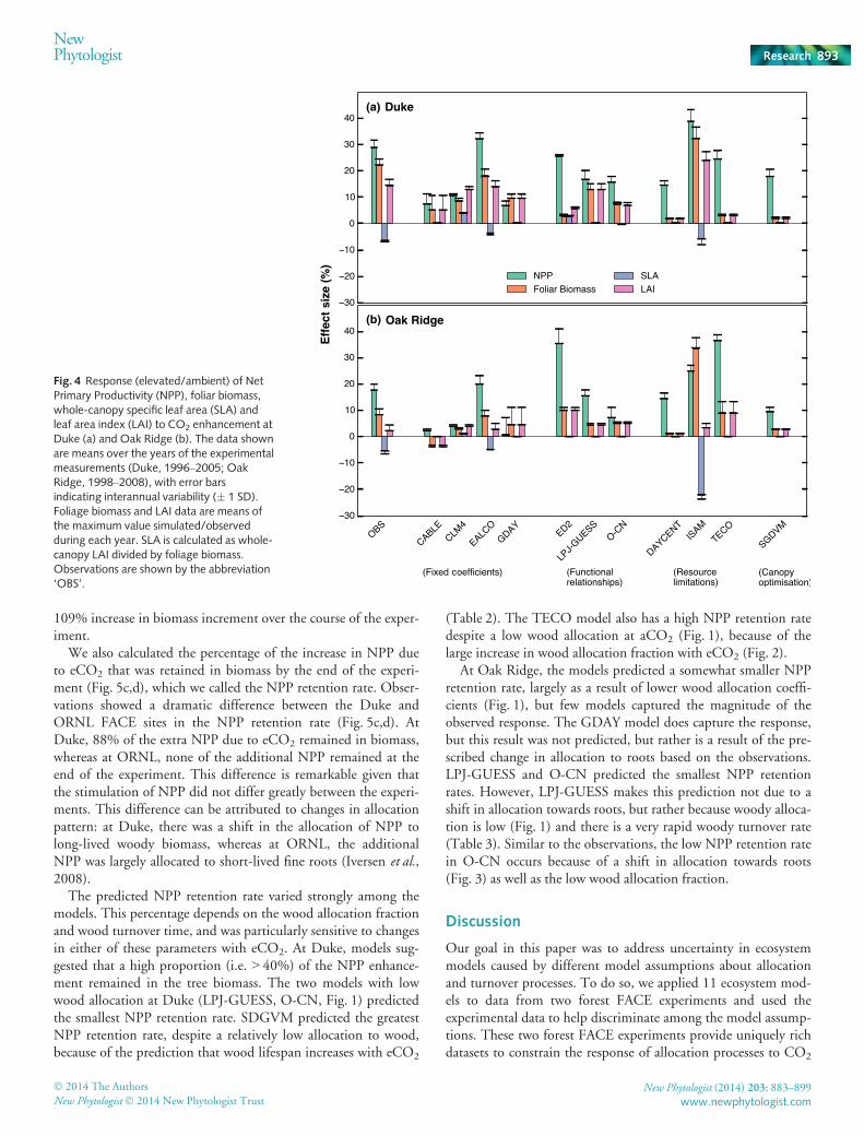
and, third, on any change in specific leaf area (SLA) with eCO2.Fig. 4 shows the observed and modelled responses of NPP,foliar biomass, SLA and LAI to eCO2. Most models predict thateCO2 leads to an increase in NPP, but there is a reduction infoliage allocation, such that the increase in foliage biomass isless than the increase in NPP. These predictions are generallyconsistent with the observations. The exception to this rule isISAM at Oak Ridge, where foliage allocation increased, asexplained above, leading to a larger response of foliage biomassthan of NPP.

Observations from both sites showed that whole-canopy SLA(calculated as total leaf area index divided by total leaf biomass)was reduced at eCO2 (�6.4 and �5.3% at Duke and Oak Ridge,respectively). Owing to this reduction in SLA, the observationsshow smaller CO2 effects on LAI (14.4% and 2.3% increase atDuke and Oak Ridge, respectively) compared to the effects onfoliage biomass (22.1% and 8.2% increase at Duke and OakRidge, respectively). By contrast, most models assume that SLAis constant, and therefore the enhancement in LAI due to CO2

directly corresponds to the foliage biomass enhancement.However, some models vary SLA. In CLM4, SLA increases as

a linear function of canopy depth (Thornton & Zimmermann,2007). Increased foliage allocation under eCO2 increases LAI,which results in a lower mean foliage C cost (increased meanSLA), allowing the enhancement in LAI to be greater than the

(a)

(b)

Fig. 1 Fractions of Net Primary Productivity(NPP) allocated at ambient CO2 to thefoliage, wood, fine roots and reproduction at(a) Duke and (b) Oak Ridge. The valuesshown are means of the annual values andthe error bars show the interannual variabilityin allocation fractions (� 1SD) calculatedover the number of years (n) of theexperiment (n = 10 at Duke and n = 11 atOak Ridge). Models are grouped byallocation model type. Observations areshown by the abbreviation ‘OBS’. Furtherdiscussion of differences among modelpredictions of allocation patterns at ambientCO2 concentration is provided in Table 1 andin Supporting Information Notes S2.



Research

NewPhytologist890

corresponding foliar biomass enhancement. This response ofSLA is in the opposite direction to observations; data at both sitesindicate a reduction in SLA at eCO2. In the ISAM model, LAI isdecoupled from canopy biomass. The LAI is calculated based ona phenological model where the maximum LAI is specified, andhas no relationship with the foliage biomass. As a consequence,the implied SLA can change dramatically with eCO2, as at OakRidge where foliage biomass is predicted to increase considerablybut prescribed LAI does not (Fig. 4). In the EALCO model, SLAis forced to decrease at eCO2 by a percentage that is based onobservations. By including this observation into the model proce-dure, the EALCO model is able to replicate the CO2 effects onboth foliage biomass and LAI (Fig. 4).

Biomass turnover

The eCO2 effect on biomass C storage depends both on alloca-tion patterns and turnover times. We therefore documented theturnover times for different plant tissues in both observations andmodels (Tables 2, 3). In comparing model turnover times toobservations, it is important to bear in mind that observed turn-over times are calculated from the turnover and mortality of

tissue during the experimental period only. During this period,woody turnover mainly reflects branch shedding and a loss ofheavily suppressed trees, and for this reason is likely to be longerthan turnover times calculated over the whole lifetime of thesespecies. Foliage and fine-root tissue have longer turnover times atDuke than at Oak Ridge. At both sites there was a noticeableCO2 effect on the lifespan of fine roots, although root lifespandecreased overall at Duke, whereas at Oak Ridge root lifespanincreased at eCO2, likely because of deeper rooting distributions(Iversen et al., 2008).

This suite of models poorly replicated the observed tissue life-spans during the experimental period (Tables 2 and 3), with con-siderable variability across sites and among models, for all tissues.Many models tended to suggest shorter woody tissue lifespanthan the observed, including CABLE, CLM4, GDAY, ISAM andSDGVM at Duke and CABLE, CLM4, DAYCENT, GDAY,ISAM, LPJ-GUESS, SDGVM and ISAM at Oak Ridge. Ashorter lifespan is to be expected in models that set turnover ratesbased on the full lifetime of woody species. For example, GDAYand TECO have shorter woody lifespans than the observationsbecause these models used general model parameterisations. Sim-ilarly, the DAYCENT model predicted woody turnover times

(a)

(b)

(c)

(d)

Fig. 2 Change in the percentage of annualNet Primary Productivity (NPP) allocated tothe foliage (green line), wood (orange line)and fine roots (blue line) between ambientand elevated CO2 at Duke.





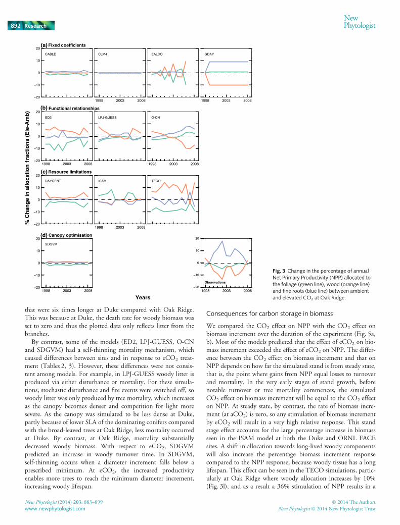
that were six times longer at Duke compared with Oak Ridge.This was because at Duke, the death rate for woody biomass wasset to zero and thus the plotted data only reflects litter from thebranches.

By contrast, some of the models (ED2, LPJ-GUESS, O-CNand SDGVM) had a self-thinning mortality mechanism, whichcaused differences between sites and in response to eCO2 treat-ment (Tables 2, 3). However, these differences were not consis-tent among models. For example, in LPJ-GUESS woody litter isproduced via either disturbance or mortality. For these simula-tions, stochastic disturbance and fire events were switched off, sowoody litter was only produced by tree mortality, which increasesas the canopy becomes denser and competition for light moresevere. As the canopy was simulated to be less dense at Duke,partly because of lower SLA of the dominating conifers comparedwith the broad-leaved trees at Oak Ridge, less mortality occurredat Duke. By contrast, at Oak Ridge, mortality substantiallydecreased woody biomass. With respect to eCO2, SDGVMpredicted an increase in woody turnover time. In SDGVM,self-thinning occurs when a diameter increment falls below aprescribed minimum. At eCO2, the increased productivityenables more trees to reach the minimum diameter increment,increasing woody lifespan.

Consequences for carbon storage in biomass

We compared the CO2 effect on NPP with the CO2 effect onbiomass increment over the duration of the experiment (Fig. 5a,b). Most of the models predicted that the effect of eCO2 on bio-mass increment exceeded the effect of eCO2 on NPP. The differ-ence between the CO2 effect on biomass increment and that onNPP depends on how far the simulated stand is from steady state,that is, the point where gains from NPP equal losses to turnoverand mortality. In the very early stages of stand growth, beforenotable turnover or tree mortality commences, the simulatedCO2 effect on biomass increment will be equal to the CO2 effecton NPP. At steady state, by contrast, the rate of biomass incre-ment (at aCO2) is zero, so any stimulation of biomass incrementby eCO2 will result in a very high relative response. This standstage effect accounts for the large percentage increase in biomassseen in the ISAM model at both the Duke and ORNL FACEsites. A shift in allocation towards long-lived woody componentswill also increase the percentage biomass increment responsecompared to the NPP response, because woody tissue has a longlifespan. This effect can be seen in the TECO simulations, partic-ularly at Oak Ridge where woody allocation increases by 10%(Fig. 3l), and as a result a 36% stimulation of NPP results in a

(a)

(b)

(c)

(d)

Fig. 3 Change in the percentage of annualNet Primary Productivity (NPP) allocated tothe foliage (green line), wood (orange line)and fine roots (blue line) between ambientand elevated CO2 at Oak Ridge.



Research

NewPhytologist892

109% increase in biomass increment over the course of the exper-iment.

We also calculated the percentage of the increase in NPP dueto eCO2 that was retained in biomass by the end of the experi-ment (Fig. 5c,d), which we called the NPP retention rate. Obser-vations showed a dramatic difference between the Duke andORNL FACE sites in the NPP retention rate (Fig. 5c,d). AtDuke, 88% of the extra NPP due to eCO2 remained in biomass,whereas at ORNL, none of the additional NPP remained at theend of the experiment. This difference is remarkable given thatthe stimulation of NPP did not differ greatly between the experi-ments. This difference can be attributed to changes in allocationpattern: at Duke, there was a shift in the allocation of NPP tolong-lived woody biomass, whereas at ORNL, the additionalNPP was largely allocated to short-lived fine roots (Iversen et al.,2008).

The predicted NPP retention rate varied strongly among themodels. This percentage depends on the wood allocation fractionand wood turnover time, and was particularly sensitive to changesin either of these parameters with eCO2. At Duke, models sug-gested that a high proportion (i.e. > 40%) of the NPP enhance-ment remained in the tree biomass. The two models with lowwood allocation at Duke (LPJ-GUESS, O-CN, Fig. 1) predictedthe smallest NPP retention rate. SDGVM predicted the greatestNPP retention rate, despite a relatively low allocation to wood,because of the prediction that wood lifespan increases with eCO2

(Table 2). The TECO model also has a high NPP retention ratedespite a low wood allocation at aCO2 (Fig. 1), because of thelarge increase in wood allocation fraction with eCO2 (Fig. 2).

At Oak Ridge, the models predicted a somewhat smaller NPPretention rate, largely as a result of lower wood allocation coeffi-cients (Fig. 1), but few models captured the magnitude of theobserved response. The GDAY model does capture the response,but this result was not predicted, but rather is a result of the pre-scribed change in allocation to roots based on the observations.LPJ-GUESS and O-CN predicted the smallest NPP retentionrates. However, LPJ-GUESS makes this prediction not due to ashift in allocation towards roots, but rather because woody alloca-tion is low (Fig. 1) and there is a very rapid woody turnover rate(Table 3). Similar to the observations, the low NPP retention ratein O-CN occurs because of a shift in allocation towards roots(Fig. 3) as well as the low wood allocation fraction.

Discussion

Our goal in this paper was to address uncertainty in ecosystemmodels caused by different model assumptions about allocationand turnover processes. To do so, we applied 11 ecosystem mod-els to data from two forest FACE experiments and used theexperimental data to help discriminate among the model assump-tions. These two forest FACE experiments provide uniquely richdatasets to constrain the response of allocation processes to CO2

(a)

(b)

Fig. 4 Response (elevated/ambient) of NetPrimary Productivity (NPP), foliar biomass,whole-canopy specific leaf area (SLA) andleaf area index (LAI) to CO2 enhancement atDuke (a) and Oak Ridge (b). The data shownare means over the years of the experimentalmeasurements (Duke, 1996–2005; OakRidge, 1998–2008), with error barsindicating interannual variability (� 1 SD).Foliage biomass and LAI data are means ofthe maximum value simulated/observedduring each year. SLA is calculated as whole-canopy LAI divided by foliage biomass.Observations are shown by the abbreviation‘OBS’.





in ecosystem models. Much of our previous understanding ofallocation responses to eCO2 has come from meta-analysis usingpredominantly potted plants (Curtis & Wang, 1998; Poorter

et al., 2012). For example, Curtis & Wang (1998) found littleevidence for sustained shifts in belowground allocation patternsdue to CO2. Similarly, Poorter et al. (2012) found little evidenceof a consistent CO2 effect on C allocation fractions (leaf, woodand roots) from a meta-analysis of young plants grown undercontrolled conditions. However, ecosystem models need to beinformed by allocation patterns at ecosystem scale, rather thanthose in rapidly expanding young plants, where ontogeneticeffects tend to outweigh environmental factors. Furthermore, toprovide strong constraints on model behaviour, we need data onallocation patterns in response to experimental manipulationsthat are accompanied by detailed information on plant nutrientand water status. The intensively-studied FACE experiments arethus of tremendous value for evaluation of allocation models.

Nonetheless, it is important to recognise the limits to whichthese data can constrain models. First, there are significant uncer-tainties in the data due to the inherent difficulty of estimatingbiomass production in large forests. For example, estimates ofwoody biomass production were made using allometric equationsdetermined from trees harvested before the onset of treatments.Root biomass production estimates were made by scaling mea-surements of root length measured using minirhizotron technol-ogy to root biomass (Iversen et al., 2008; Pritchard et al., 2008).Second, there were a number of one-off events that likely affectedallocation patterns in the experiments, but were not related toatmospheric CO2 and are not captured in models. These eventsinclude a windstorm at Oak Ridge in 2004 and an ice storm atDuke in 2002 (McCarthy et al., 2006). Third, changes in alloca-tion patterns in the models are intended to represent responses togradual changes rather than the step increase in CO2 concentra-tion applied in the experiments. Furthermore, most models wereparameterised with standard PFT parameters rather than site-spe-cific parameters. Also, at the Duke site, the significant hardwoodunderstorey is ignored by most models, which simulate pinesonly. For these reasons, we should not expect any model to pre-cisely match the observed magnitude and interannual variabilityof treatment effects on allocation. Rather, we assessed the capac-ity of the models to qualitatively reproduce the major features ofthe observed changes. The overall effects of CO2 treatment onallocation patterns were clear, but differed between the two sites,with N availability as an important driver (Finzi et al., 2007;Norby et al., 2010; Zaehle et al., 2014).

Comparative success of different allocation models

We examined four different classes of allocation assumption.Broadly speaking, the models that used functional relationshipsamong biomass fractions to control C allocation (ED2, LPJ-GUESS, O-CN) were best able to replicate the contrastingobserved changes in C partitioning at eCO2 at both sites. Thesemodels initially predicted an increase in wood allocation witheCO2 in line with the observations, but as these models becamewater and nutrient stressed, allocation shifted towards roots.Thus, both the allometry of leaf to wood biomass, and the shiftin the functional relationship between leaf and root biomass withstress, were important to capture the CO2 response. The timing

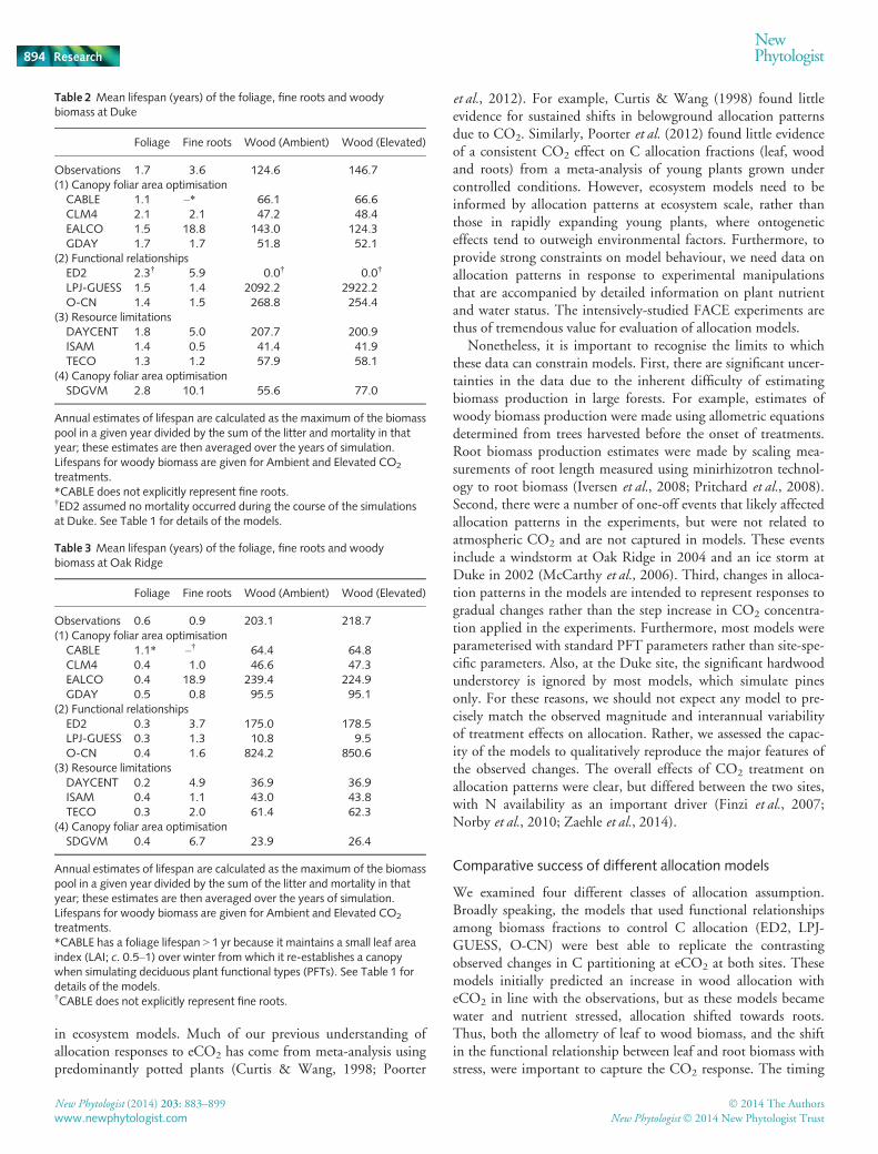
Table 2 Mean lifespan (years) of the foliage, fine roots and woodybiomass at Duke

Foliage Fine roots Wood (Ambient) Wood (Elevated)

Observations 1.7 3.6 124.6 146.7(1) Canopy foliar area optimisationCABLE 1.1 –* 66.1 66.6CLM4 2.1 2.1 47.2 48.4EALCO 1.5 18.8 143.0 124.3GDAY 1.7 1.7 51.8 52.1

(2) Functional relationshipsED2 2.3† 5.9 0.0† 0.0†

LPJ-GUESS 1.5 1.4 2092.2 2922.2O-CN 1.4 1.5 268.8 254.4

(3) Resource limitationsDAYCENT 1.8 5.0 207.7 200.9ISAM 1.4 0.5 41.4 41.9TECO 1.3 1.2 57.9 58.1

(4) Canopy foliar area optimisationSDGVM 2.8 10.1 55.6 77.0

Annual estimates of lifespan are calculated as the maximum of the biomasspool in a given year divided by the sum of the litter and mortality in thatyear; these estimates are then averaged over the years of simulation.Lifespans for woody biomass are given for Ambient and Elevated CO2

treatments.*CABLE does not explicitly represent fine roots.†ED2 assumed no mortality occurred during the course of the simulationsat Duke. See Table 1 for details of the models.

Table 3 Mean lifespan (years) of the foliage, fine roots and woodybiomass at Oak Ridge

Foliage Fine roots Wood (Ambient) Wood (Elevated)

Observations 0.6 0.9 203.1 218.7(1) Canopy foliar area optimisationCABLE 1.1* –† 64.4 64.8CLM4 0.4 1.0 46.6 47.3EALCO 0.4 18.9 239.4 224.9GDAY 0.5 0.8 95.5 95.1

(2) Functional relationshipsED2 0.3 3.7 175.0 178.5LPJ-GUESS 0.3 1.3 10.8 9.5O-CN 0.4 1.6 824.2 850.6

(3) Resource limitationsDAYCENT 0.2 4.9 36.9 36.9ISAM 0.4 1.1 43.0 43.8TECO 0.3 2.0 61.4 62.3

(4) Canopy foliar area optimisationSDGVM 0.4 6.7 23.9 26.4

Annual estimates of lifespan are calculated as the maximum of the biomasspool in a given year divided by the sum of the litter and mortality in thatyear; these estimates are then averaged over the years of simulation.Lifespans for woody biomass are given for Ambient and Elevated CO2

treatments.*CABLE has a foliage lifespan > 1 yr because it maintains a small leaf areaindex (LAI; c. 0.5–1) over winter from which it re-establishes a canopywhen simulating deciduous plant functional types (PFTs). See Table 1 fordetails of the models.†CABLE does not explicitly represent fine roots.



Research

NewPhytologist894

of the development of stress responses varied between the modelsand differed from observations (see Zaehle et al., 2014), but theydid tend to capture the direction of allocation shifts due to eCO2.The success of these schemes is in contrast to previous work byLuo et al. (1994), who found that a model built on the principlesof the functional balance hypothesis did a poor job of explainingobserved changes in root allocation in response to eCO2. How-ever, this study concerned young plants aged 22 d to 27 months.In addition, a key assumption of the model used by Luo et al.(1994) was that total N uptake did not change in response toCO2 treatment, as was observed in the experiments they consid-ered. By contrast, N uptake increased at eCO2 in both of theFACE sites studied here (Finzi et al., 2007). Thus, the functionalbalance approach appears to be more successful for explainingthe CO2 effects on allocation in forest ecosystems than in youngplants.

By comparison to the observations, modelled changes in allo-cation patterns were more gradual, meaning that they did notmatch the observed interannual variability in the observations.The models show a lagged response of allocation to changes inwater and nutrient limitations (due to annual allocation in LPJ-GUESS, and a time-integrated N scalar in O-CN), which buffersthe rate at which allocation to roots changes. However, asexplained above, we would not necessarily expect the models tobe able to simulate responses to step changes in environmentalconditions. Of more concern is the fact that different

parameterisations among these models resulted in marked differ-ences among otherwise similar schemes (see Notes S2), indicatingthat parameterisation of these schemes is a source of significantuncertainty. Large-scale synthesis of data on allocation patterns(Litton et al., 2007; Wolf et al., 2011a,b) could potentially beused to reduce this uncertainty, particularly if synthesis was donein terms of model parameters.

The other three approaches used to represent allocation in ourecosystem models were considerably less successful at reproduc-ing observations. Of particular concern, allocation schemes inwhich the allocation coefficients were not constrained by theresulting biomass fractions (i.e. constant coefficient and resourcelimitation approaches) could have unintended outcomes. Forexample, due to the interaction of allocation with a phenologicalscheme, CABLE unexpectedly predicted an eCO2 effect on Callocation to wood during a drought at Duke. Similarly, inISAM, a maximum LAI was prescribed, causing leaf senescencein eCO2 to be delayed by as much as 20 d, with the unintendedresult of increased partitioning to foliage at eCO2 at ORNL.These results show that allocation schemes either need to be con-strained by the resultant biomass fractions (e.g. the functionalrelationships approach) or tested thoroughly to ensure that modelpredictions are as intended.

The constant allocation coefficient approach (CABLE, CLM4,EALCO, GDAY) is unsuitable for predicting the consequencesof eCO2 for allocation because it is unable to capture dynamic

(a)

(b)

(c)

(d)

Fig. 5 The effect of CO2 enhancement onvegetation carbon storage at the two sites.Left-hand plots show the effect of elevatedCO2 on cumulative Net Primary Productivity(NPP; red bars) and biomass increment (bluebars) over the experiment at (a) Duke and (b)Oak Ridge. Right-hand plots show theproportion of additional NPP resulting fromthe increase in CO2 which remains in theplant biomass (foliage, wood and fine roots)at the end of the experiment at (c) Duke and(d) Oak Ridge. Note the bar for TECO inpanel (b) has been clipped to 100% forplotting purposes, but extends to 109%.Observations are shown by the abbreviation‘OBS’.





changes in allocation with changing water and nutrient availabil-ity at seasonal to interannual timescales. The experimental datashow that these shifts in allocation pattern are significant, andtherefore need to be captured in models, although it remainsuncertain whether these changes in allocation pattern will be per-sistent over the long term.

The resource limitation approach – in which allocation frac-tions are decided based on the relative strength of nutrient, water,and light limitations – is similar in some ways to the functionalrelationships approach, but the models were significantly less suc-cessful at predicting the observed allocation patterns. This lack ofsuccess may be due to the fact that the approach is based on allo-cation fractions, which are considerably more difficult to measurethan biomass fractions, with the consequence that many fewerdata are available on which to base model formulations andparameters. In addition, at least some of the available data avail-able do not support the general approach of prioritisation amongplant components used in DAYCENT and TECO (Litton et al.,2007).

The one optimisation approach to allocation included in ourset of 11 models (SDGM) also failed to capture the observedresponses. However, this was principally because the optimisationapproach was incomplete, combining foliar optimisation withfixed coefficients for wood and root tissues. A number of otheroptimisation and game-theoretic allocation models have beendeveloped (e.g. see Franklin et al., 2012). Several of theseapproaches have given promising results for explaining observedpatterns in C allocation (Dewar et al., 2009; Dybzinski et al.,2011; Valentine & M€akel€a, 2012; McMurtrie & Dewar, 2013)including observations from FACE experiments (Franklin et al.,2009; McMurtrie et al., 2012). The results from these studies aresufficiently promising to merit investigation of the implicationsof these concepts when implemented into ecosystem models. Itwould be particularly useful to implement the ‘assumption-cen-tred’ model evaluation framework developed here to investigatehow such models compare to the allocation models currently inuse.

Other important processes

In addition to allocation, tissue turnover is a key process deter-mining C storage in biomass, particularly turnover rates of thelong-lived woody biomass (Bugmann & Bigler, 2011; Smithet al., 2013; Xia et al., 2013). Very few of the models consideredhere include any explicit mechanism governing turnover. Tissuelifespan is usually a prescribed parameter, either by PFT or basedon site knowledge. Elevated CO2 has been shown to affect tissuelifespan. For example, needle lifespan was reduced at DukeFACE (Sch€afer et al., 2002) and root lifespan was increased atORNL FACE (Iversen et al., 2008). This CO2-induced responsehas implications for short-term litterfall and long-term soil Cstorage (see Iversen et al., 2012). Even the models that employeda mechanism to adjust lifespan still did not compare well to data:LPJ-GUESS and SDGVM produced very different and at timesunrealistic results when applied to a transient step-change experi-ment. Amongst models in which turnover processes are

parameterised, there was striking inter-model variability in thelifespan of the wood, foliage and fine roots (Tables 2, 3); it variesby as much as an order of magnitude for the woody component.These results point to a need for better data on turnover. Suchdata could come from many sources besides manipulative CO2

experiments. In particular, they need to cover all stages in forestdevelopment (Wolf et al., 2011b).

Similarly, to estimate CO2 effects on canopy cover, modelsneed to estimate SLA in addition to foliage allocation. Mostmodels prescribed SLA and therefore did not capture theobserved reduction in SLA due to eCO2. As a consequence,changes in canopy cover in response to eCO2 are overestimated.However, the only model currently incorporating a theoreticalprediction of SLA (CLM-CN) performed worse, because SLAwas predicted to increase rather than decrease. A reduction inSLA is a commonly observed response in eCO2 experiments(Medlyn et al., 1999; Ainsworth & Long, 2005; Poorter et al.,2009) that needs to be incorporated in ecosystem models, prefer-ably via a process-based prediction of SLA rather than an ad hocreduction in SLA as CO2 increases. SLA is one of the most com-monly studied plant traits (Kattge et al., 2011), so there are ampledata available on which to base such a model.

Where does the carbon go?

The observed site responses show contrasting effects of eCO2 onthe fate of vegetation C. There was a sustained increase in bio-mass C at Duke FACE but no sustained increase at ORNLFACE. In both cases, models were unable to correctly simulatethe change in C storage, because they were unable to capture thefull extent of the site N dynamics (see Zaehle et al., 2014) andthe resulting change in allocation patterns. At Duke FACE, mod-els tended to predict that a greater proportion of the enhance-ment in NPP remained in the plant biomass at the end of theexperiment than the observations indicated. In many cases (DAY-CENT, EALCO, ED2, LPJ-GUESS and O-CN), this wasbecause the models prescribed too long a turnover time for wood,and allocated too much of the additional NPP to wood. Theresponse was more variable at Oak Ridge, but models again over-predicted the resulting change in plant biomass (with the excep-tion of GDAY, which used prescribed allocation). At both sites,therefore, models generally over-predicted the C storage due toeCO2.

Soil is also a major store for carbon. We did not address theCO2 effect on C storage in the soil, as we were focusing on modelassumptions related to biomass allocation and turnover. Predic-tions of soil C storage will be influenced by the input of C to soil,which is dependent on assumptions about allocation, especiallyto fine roots (Iversen et al. 2012), but the fate of C in soil dependson a different set of model assumptions that are chiefly related toorganic matter decomposition. Future work should investigatehow these assumptions differ among models and the interactionbetween plant allocation and soil processes. Constraining theseassumptions with data will be challenging, given the inherentuncertainty in soil C data (Hungate et al., 2009). Even after adecade of experimentation, soil C changes in the two FACE



Research

NewPhytologist896

experiments are difficult to detect because of the large, heteroge-neous background pool.

We also do not address the allocation of photosynthate to pro-cesses other than growth and respiration. These processes includeC exudation to the rhizosphere, transfer to mycorrhizae, volatileorganic C emissions, and losses to herbivory. These C flows mayhave important ecosystem consequences; for example, rhizo-sphere C inputs are thought to increase with eCO2, stimulatingmicrobial activity and enhancing plant available N (Drake et al.,2011; Phillips et al., 2012). However, these fluxes have not beenquantified directly for the two FACE sites, and estimates haveprincipally been inferred from mass balance calculations (Palm-roth et al., 2006; Drake et al., 2011; Phillips et al., 2011). Fur-thermore, none of the models considered here have anymechanistic representation of rhizodeposition processes. Conse-quently, these additional C flows remain a key unknown requir-ing additional experimental data and model development.

Some of the models (ED2, LPJ-GUESS and O-CN) didinclude allocation of C to reproduction. Where these fluxes weresimulated, they were considerably larger than observed. In thecase of ED2, for example, the allocation fraction to reproductionwas 16–22% and increased by 6–12% with eCO2. By contrast,the observed allocation to reproduction was <1% at Duke(McCarthy et al., 2010). The sweetgum trees at ORNL did notproduce measurable reproductive tissue within the timeframe ofthe experiment.

Ways to reduce model uncertainty

This study has shown that model uncertainty due to allocationand turnover processes could be reduced through several means,including improvements to models, targeted synthesis of experi-mental data and additional measurements.

We have shown that allocation approaches that are constrainedby biomass fractions (such as functional relationships) were moresuccessful at capturing observed trends, and were generally morerobust, than approaches based on allocation coefficients. In par-ticular, we showed that approaches using constant allocationcoefficients or resource limitations, when combined with pheno-logical schemes occasionally produced unintended responses toeCO2. We therefore advocate allocation approaches based onfunctional relationships or optimisation schemes, and that anyallocation model should be subjected to wide-ranging tests to dis-cover whether it behaves as intended.

We have shown that allocation parameters differ considerablyamong models. Synthesis of existing allocation data, especially ifit is done in terms of model parameters, would reduce uncer-tainty among models by providing baseline parameter values.Similarly, we showed that turnover coefficients were highly vari-able among models, indicating that they are poorly constrainedby data. Uncertainty among models could be reduced with bettermeasurements of turnover, as well as synthesis of existing mea-surements. Such work could also assist in developing better mod-els of turnover. SLA has been extensively measured, and thesemeasurements should be used to help develop process representa-tion for environmental effects on SLA.

FACE experiments provide rich datasets with which to con-strain models, but the strongly contrasting responses between thetwo experimental sites imply that additional datasets will beneeded to derive generalisations about allocation at the ecosystemscale. Ecosystem manipulation experiments need to be intensivelystudied to provide all the data needed to constrain models. Forthe work presented here we required data on growth and turnoverof all plant components as well as complementary data on plantwater and nutrient availability. We recommend that future eco-system-scale experiments attempt to fully quantify carbon, waterand nutrient budgets.

Acknowledgements

This work was conducted as a part of the ‘Benchmarking ecosys-tem response models with experimental data from long-termCO2 enrichment experiments’ Working Group supported by theNational Center for Ecological Analysis and Synthesis, a Centerfunded by NSF (Grant #EF-0553768), the University of Califor-nia, Santa Barbara, and the State of California. The Oak Ridgeand Duke FACE sites and additional synthesis activities weresupported by the US Department of Energy Office of Science,Biological and Environmental Research Program. M.G.D.K. wassupported by ARC Discovery Grant DP1094791. S.Z. was sup-ported by the European Community’s Seventh FrameworkProgramme FP7 people programme through grants’ noPERG02-GA-2007-224775 and 238366. T.H. was fundedthrough the LOEWE initiative for scientific and economic excel-lence of the German federal state of Hesse. D.W. and B.S. con-tribute to the strategic research areas BECC, MERGE andLUCCI.

References

Abramowitz G, Leuning R, Clark M, Pitman A. 2008. Evaluating the

performance of Land Surface Models. Journal of Climate 21: 5468–5481.Ainsworth EA, Long SP. 2005.What have we learned from 15 years of free-air

CO2 enrichment (FACE)? A meta-analytic review of the responses of

photosynthesis, canopy properties and plant production to rising CO2. NewPhytologist 165: 351–372.

Arora VK, Boer GJ. 2005. A parameterization of leaf phenology for the terrestrial

ecosystem component of climate models. Global Change Biology 11: 39–59.Arora VK, Boer GJ, Friedlingstein P, Eby M, Jones CD, Christian JR, Bonan G,

Bopp L, Brovkin V, Cadule P et al. 2013. Carbon-concentration and

carbon-climate feedbacks in CMIP5 Earth system models. Journal of Climate26: 5289–5314.

Bonan GB. 2008. Forests and climate change: forcings, feedbacks, and the

climate benefits of forests. Science 320: 1444–1449.Bugmann H, Bigler C. 2011.Will the CO₂ fertilization effect in forests be offset

by reduced tree longevity? Oecologia 165: 533–544.Canadell JG, Le Qu�er�e C, Raupach MR, Field CB, Buitenhuis ET, Ciais P,

Conway TJ, Gillett NP, Houghton RA, Marland G. 2007. Contributions to

accelerating atmospheric CO2 growth from economic activity, carbon intensity,

and efficiency of natural sinks. Proceedings of the National Academy of Sciences,USA 104: 18 866–18 870.

Cox PM, Betts RA, Jones CD, Spall SA, Totterdell IJ. 2000. Acceleration of

global warming due to carbon-cycle feedbacks in a coupled climate model.

Nature 408: 184–187.Cramer W, Bondeau A, Woodward I, Prentice C, Betts RA, Brovkin V, Cox

PM, Fisher V, Foley JA, Friend AD et al. 2001. Global response of terrestrial





ecosystem structure and function to CO2 and climate change: results from six

dynamic global vegetation models. Global Change Biology 7: 357–373.Curtis PS, Wang X. 1998. A meta-analysis of elevated CO₂ effects on woody

plant mass, form, and physiology. Oecologia 113: 299–313.Davidson R. 1969. Effect of root/leaf temperature differentials on root/shoot

ratios in some pasture grasses and clover. Annals of Botany 33: 561–569.De Kauwe MG, Medlyn BE, Zaehle S, Walker AP, Dietze MC, Hickler T, Jain

AK, Luo Y, Parton WJ, Prentice C et al. 2013. Forest water use and water use

efficiency at elevated CO2: a model–data intercomparison at two contrasting

temperate forest FACE sites. Global Change Biology 19: 1759–1779.Dewar RC, Franklin O, M€akel€a A, McMurtrie RE, Valentine HT. 2009.

Optimal function explains forest responses to global change. BioScience 59:127–139.

Drake JE, Gallet-Budynek A, Hofmockel KS, Bernhardt ES, Billings SA,

Jackson RB, Johnsen KS, Lichter J, McCarthy HR, McCormack ML et al.2011. Increases in the flux of carbon belowground stimulate nitrogen uptake

and sustain the long-term enhancement of forest productivity under elevated

CO₂. Ecology Letters 14: 349–357.Dybzinski R, Farrior C, Wolf A, Reich PB, Pacala SW. 2011. Evolutionarily

stable strategy carbon allocation to foliage, wood, and fine roots in trees

competing for light and nitrogen: an analytically tractable, individual-based

model and quantitative comparisons to data. American Naturalist 177: 153–166.Farrior CE, Dybzinski R, Levin SA, Pacala SW. 2013. Competition for water

and light in closed-canopy forests: a tractable model of carbon allocation with

implications for carbon sinks. American Naturalist 181: 314–330.Finzi AC, Norby RJ, Calfapietra C, Gallet-Budynek A, Gielen B, Holmes WE,

Hoosbeek MR, Iversen CM, Jackson RB, Kubiske ME et al. 2007. Increasesin nitrogen uptake rather than nitrogen-use efficiency support higher rates of

temperate forest productivity under elevated CO₂. Proceedings of the NationalAcademy of Sciences, USA 104: 14 014–14 019.

Franklin O, Johansson J, Dewar RC, Dieckmann U, McMurtrie RE,

Br€annst€om�A, Dybzinski R. 2012.Modeling carbon allocation in trees: a

search for principles. Tree Physiology 32: 648–666.Franklin O, McMurtrie RE, Iversen CM, Crous KY, Finzi AC, Tissue DT,

Ellsworth DS, Oren R, Norby RJ. 2009. Forest fine-root production and

nitrogen use under elevated CO₂: contrasting responses in evergreen and

deciduous trees explained by a common principle. Global Change Biology 15:132–144.

Friedlingstein P, Cox P, Betts R, Bopp L, Von Bloh W, Brovkin V, Cadule P,

Doney S, Eby M, Fung I et al. 2006. Climate-carbon cycle feedback analysis:

results from the C4MIP model intercomparison. Journal of Climate 19: 3337–3353.

Friedlingstein P, Joel G, Field C, Fung I. 1999. Toward an allocation scheme for

global terrestrial carbon models. Global Change Biology 5: 755–770.Friend AD, Lucht W, Rademacher TT, Keribin R, Betts R, Cadule P, Ciais P,

Clark DB, Dankers R, Falloon PD et al. 2014. Carbon residence time

dominates uncertainty in terrestrial vegetation responses to future climate and

atmospheric CO2. Proceedings of the National Academy of Sciences, USA 111:

3280–3285.Hungate BA, van Groenigen KJ, Six J, Jastrow JD, Luo Y, de Graaff MA, van

Kessel C, Osenberg CW. 2009. Assessing the effect of elevated CO2 on soil C:

a comparison of four meta-analyses. Global Change Biology 15: 2020–2034.Ise T, Litton CM, Giardina CP, Ito A. 2010. Comparison of modeling

approaches for carbon partitioning: impact on estimates of global net primary

production and equilibrium biomass of woody vegetation from MODIS GPP.

Journal of Geophysical Research 115: G04025.Iversen CM, Keller JK, Garten CT, Norby RJ. 2012. Soil carbon and nitrogen

cycling and storage throughout the soil profile in a sweetgum plantation after

11 years of CO2-enrichment. Global Change Biology 18: 1684–1697.Iversen CM, Ledford J, Norby RJ. 2008. CO2 enrichment increases carbon and

nitrogen input from fine roots in a deciduous forest. New Phytologist 179: 837–847.

Jones C, Robertson E, Arora V, Friedlingstein P, Shevliakova E, Bopp L,

Brovkin V, Hajima T, Kato E, Kawamiya M et al. 2013. Twenty-first-centurycompatible CO2 emissions and airborne fraction simulated by CMIP5 earth

system models under four representative concentration pathways. Journal ofClimate 26: 4398–4413.

Kattge J, Diaz S, Lavorel S, Prentice I, Leadley P, B€onisch G, Garnier E,

Westoby M, Reich PB, Wright I et al. 2011. TRY–a global database of planttraits. Global Change Biology 17: 2905–2935.

Kimball BA. 1983. Carbon dioxide and agricultural yield: an assemblage and

analysis of 430 prior observations. Agronomy Journal 75: 779–788.Korner C, Asshoff R, Bignucolo O, H€attenschwiler S, Keel SG, Pel�aez-Riedl S,Pepin S, Siegwolf RT, Zotz G. 2005. Carbon flux and growth in mature

deciduous forest trees exposed to elevated CO2. Science 309: 1360–1362.Le Qu�er�e C, Andres RJ, Boden T, Conway T, Houghton R, House JI, Marland

G, Peters GP, van der Werf G, Ahlstr€om A et al. 2013. The global carbonbudget 1959–2011. Earth System Science Data 5: 165–185.

Le Qu�er�e C, Raupach MR, Canadell JG, Marland G, Bopp L, Ciais P, Conway

TJ, Doney SC, Feely RA, Foster P et al. 2009. Trends in the sources and sinks

of carbon dioxide. Nature Geoscience 2: 831–836.Lenton T, Williamson M, Edwards N, Marsh R, Price A, Ridgwell A, Shepherd

J, Cox S. 2006.Millennial timescale carbon cycle and climate change in an

efficient Earth system model. Climate Dynamics 26: 687–711.Litton CM, Raich JW, Ryan MG. 2007. Carbon allocation in forest ecosystems.

Global Change Biology 13: 2089–2109.Luo Y, Field C, Mooney H. 1994. Predicting responses of photosynthesis and

root fraction to elevated [CO2]a: interactions among carbon, nitrogen, and

growth. Plant, Cell & Environment 17: 1195–1204.Luo Y, Su B, Currie W, Dukes J, Finzi A, Hartwig U, Hungate B, McMurtrie

R, Oren R, Parton W et al. 2004. Progressive nitrogen limitation of ecosystem

responses to rising atmospheric carbon dioxide. BioScience 54: 731–739.Luo Y, White LW, Canadell JG, DeLucia EH, Ellsworth DS, Finzi A, Lichter J,

Schlesinger WH. 2003. Sustainability of terrestrial carbon sequestration: a case

study in Duke Forest with inversion approach. Global Biogeochemical Cycles 17:1021.

McCarthy HR, Oren R, Finzi AC, Ellsworth DS, Kim HS, Johnsen KH, Millar

B. 2007. Temporal dynamics and spatial variability in the enhancement of

canopy leaf area under elevated atmospheric CO2. Global Change Biology 13:2479–2497.

McCarthy HR, Oren R, Johnsen KH, Gallet-Budynek A, Pritchard SG, Cook

CW, LaDeau SL, Jackson RB, Finzi AC. 2010. Re-assessment of plant carbon

dynamics at the Duke free-air CO2 enrichment site: interactions of atmospheric

[CO2] with nitrogen and water availability over stand development. NewPhytologist 185: 514–528.

McCarthy HR, Oren R, Kim H-S, Johnsen KH, Maier C, Pritchard SG, Davis

MA. 2006. Interaction of ice storms and management practices on current

carbon sequestration in forests with potential mitigation under future CO2

atmosphere. Journal of Geophysical Research 111: D15103.

McMurtrie RE, Dewar RC. 2013.New insights into carbon allocation by trees

from the hypothesis that annual wood production is maximized. NewPhytologist 199: 981–990.

McMurtrie RE, Iversen CM, Dewar RC, Medlyn BE, N€asholm T, Pepper

DA, Norby RJ. 2012. Plant root distributions and nitrogen uptake

predicted by a hypothesis of optimal root foraging. Ecology and Evolution 2:

1235–1250.Medlyn B, Badeck F, De Pury D, Barton C, Broadmeadow M, Ceulemans R,

De Angelis P, Forstreuter M, Jach M, Kellomaki S et al. 1999. Effects ofelevated [CO2] on photosynthesis in European forest species: a meta-analysis of

model parameters. Plant, Cell & Environment 22: 1475–1495.Medlyn B, Robinson AP, Clement R, McMurtrie RE. 2005.On the validation

of models of forest CO2 exchange using eddy covariance data: some perils and

pitfalls. Tree Physiology 25: 839–857.Medvigy D, Wofsy SC, Munger JW, Hollinger DY, Moorcroft PR. 2009.

Mechanistic scaling of ecosystem function and dynamics in space and time:

Ecosystem Demography model version 2. Journal of GeophysicalResearch-Biogeosciences 114: G01002.

Moss RH, Edmonds JA, Hibbard KA, Manning MR, Rose SK, van Vuuren DP,

Carter TR, Emori S, Kainuma M, Kram T et al. 2010. The next generation of

scenarios for climate change research and assessment. Nature 463: 747–756.Norby RJ, DeLucia EH, Gielen B, Calfapietra C, Giardina CP, King JS,

Ledford J, McCarthy HR, Moore DJ, Ceulemans R et al. 2005. Forestresponse to elevated CO2 is conserved across a broad range of productivity.

Proceedings of the National Academy of Sciences, USA 102: 18 052–18 056.



Research

NewPhytologist898

Norby RJ, Ledford J, Reilly CD, Miller NE, O’Neill EG. 2004. Fine-root

production dominates response of a deciduous forest to atmospheric CO2

enrichment. Proceedings of the National Academy of Sciences, USA 101: 9689.

Norby RJ, Todd DE, Fults J, Johnson DW. 2001. Allometric determination of

tree growth in a CO2-enriched sweetgum stand. New Phytologist 150: 477–487.Norby RJ, Warren JM, Iverson CM, Medlyn BM, McMurtrie RE. 2010. CO₂enhancement of forest productivity constrained by limited nitrogen availability.

Proceedings of the National Academy of Sciences, USA 107: 19 368–19 373.Oren R, Ellsworth DS, Johnsen KH, Phillips N, Ewers BE, Maier C, Schafer

KVR, McCarthy H, Hendrey G, McNulty SG et al. 2001. Soil fertility limits

carbon sequestration by forest ecosystems in a CO₂-enriched atmosphere.

Nature 411: 469–472.Palmroth S, Oren R, McCarthy HR, Johnsen KH, Finzi AC, Butnor JR, Ryan

MG, Schlesinger WH. 2006. Aboveground sink strength in forests controls the

allocation of carbon below ground and its [CO2]-induced enhancement.

Proceedings of the National Academy of Sciences, USA 103: 19 362.

Pan Y, Birdsey RA, Fang J, Houghton R, Kauppi PE, Kurz WA, Phillips OL,

Shvidenko A, Lewis SL, Canadell JG et al. 2011. A large and persistent carbon

sink in the world’s forests. Science 333: 988–993.Phillips RP, Finzi AC, Bernhardt ES. 2011. Enhanced root exudation induces

microbial feedbacks to N cycling in a pine forest under long-term CO2

fumigation. Ecology Letters 14: 187–194.Phillips RP, Meier IC, Bernhardt ES, Grandy AS, Wickings K, Finzi AC. 2012.

Roots and fungi accelerate carbon and nitrogen cycling in forests exposed to

elevated CO2. Ecology Letters 15: 1042–1049.Poorter H, Niinemets €U, Poorter L, Wright IJ, Villar R. 2009. Causes and

consequences of variation in leaf mass per area (LMA): a meta-analysis. NewPhytologist 182: 565–588.

Poorter H, Niklas KJ, Reich PB, Oleksyn J, Poot P, Mommer L. 2012. Biomass

allocation to leaves, stems and roots: meta-analyses of interspecific variation and

environmental control. New Phytologist 193: 30–50.Pritchard SG, Strand AE, McCormack ML, Davis MA, Finzi AC, Jackson RB,

Matamala R, Rogers HH, Oren R. 2008. Fine root dynamics in a loblolly pine

forest are influenced by free-air-CO2-enrichment: a six-year-minirhizotron

study. Global Change Biology 14: 588–602.Reich PB, Hobbie SE. 2012. Decade-long soil nitrogen constraint on the CO2

fertilization of plant biomass. Nature Climate Change 3: 278–282.Sch€afer KVR, Oren R, Lai CT, Katul GG. 2002.Hydrologic balance in an intact

temperate forest ecosystem under ambient and elevated atmospheric CO2

concentration. Global Change Biology 9: 895–911.Schaphoff S, Lucht W, Gerten D, Sitch S, Cramer W, Prentice IC. 2006.

Terrestrial biosphere carbon storage under alternative climate projections.

Climatic Change 74: 97–122.Shinozaki K, Yoda K, Hozumi K, Kira T. 1964a. A quantitative analysis of plant

form-the pipe model theory: I. Basic analyses. Japanese Journal of Ecology 14:97–105.

Shinozaki K, Yoda K, Hozumi K, Kira T. 1964b. A quantitative analysis of plant

form-the pipe model theory: II. Further evidence of the theory and its

application in forest ecology. Japanese Journal of Ecology 14: 133–139.Sitch S, Smith B, Prentice IC, Arneth A, Bondeau A, Cramer W, Kaplan J,

Levis S, Lucht W, Sykes M et al. 2003. Evaluation of ecosystem dynamics,

plant geography and terrestrial carbon cycling in the LPJ Dynamic Vegetation

Model. Global Change Biology 9: 161–185.SmithB,W�arlindD,ArnethA,HicklerT, LeadleyP, Siltberg J, Zaehle S. 2014.

Implications of incorporatingNcycling andN limitations on primary production

in an individual-baseddynamic vegetationmodel.Biogeosciences11: 2027–2054.Smith M, Purves D, Vanderwel M, Lyutsarev V, Emmott S. 2013. The climate

dependence of the terrestrial carbon cycle, including parameter and structural

uncertainties. Biogeosciences 10: 583–606.

Thornley J. 1972. A balanced quantitative model for root: shoot ratios in

vegetative plants. Annals of Botany 36: 431–441.Thornton PE, Lamarque JF, Rosenbloom NA, Mahowald NM. 2007. Influence

of carbon-nitrogen cycle coupling on land model response to CO2 fertilization

and climate variability. Global Biogeochemical Cycles 21: 1–15.Thornton PE, Zimmermann NE. 2007. An improved canopy integration scheme

for a land surface model with prognostic canopy structure. Journal of Climate20: 3902–3923.

Valentine HT, M€akel€a A. 2012.Modeling forest stand dynamics from optimal

balances of carbon and nitrogen. New Phytologist 194: 961–971.Walker AP, Hanson PJ, De Kauwe MG, Medlyn BE, Zaehle S, Asao S, Dietze

M, Hickler T, Huntingford C, Iversen CM et al. 2014. Comprehensive

ecosystem model-data synthesis using multiple data sets at two temperate forest

free-air CO2 enrichment experiments: model performance at ambient CO2

concentration. Journal of Geophysical Research: Biogeosciences 119: doi: 10.1002/2013JG002553.

Wang S, Grant RF, Verseghy DL, Black TA. 2002.Modelling carbon dynamics

of boreal forest ecosystems using the Canadian Land Surface Scheme. ClimaticChange 55: 451–477.

Weng E, Luo Y. 2011. Relative information contributions of model vs. data to

short-and long-term forecasts of forest carbon dynamics. Ecological Applications21: 1490–1505.

Wolf A, Ciais P, Bellassen V, Delbart N, Field CB, Berry JA. 2011a. Forest

biomass allometry in global land surface models. Global Biogeochemical Cycles25: GB003917.

Wolf A, Field CB, Berry JA. 2011b. Allometric growth and allocation in

forests: a perspective from FLUXNET. Ecological Applications 21:1546–1556.

Xia J, Luo Y, Wang Y-P, Hararuk O. 2013. Traceable components of terrestrial

carbon storage capacity in biogeochemical models. Global Change Biology 19:2104–2116.

Zaehle S, Medlyn BE, De Kauwe MG, Walker AP, Dietze MC, Hickler T,

Luo Y, Wang Y-P, El-Masri B, Thornton P et al. 2014. Evaluating theresponses of 11 terrestrial carbon-nitrogen cycle models using observations

from two temperate Free-Air CO2 Enrichment Studies. New Phytologist 202:803–822.

Supporting Information

Additional supporting information may be found in the onlineversion of this article.

Fig. S1Modelled labile carbohydrate store at Duke and at OakRidge.

Notes S1Carbohydrate storage and remobilisation.

Notes S2Differences among model predictions of allocation pat-terns at ambient CO2 concentration.

Please note: Wiley Blackwell are not responsible for the contentor functionality of any supporting information supplied by theauthors. Any queries (other than missing material) should bedirected to the New Phytologist Central Office.





Documents

Where does the carbon go? A modeldata …Where does the carbon go? A model–data intercomparison of vegetation carbon allocation and turnover processes at two temperate forest free-air