Working Paper 276

El Niño and Indian Droughts- A Scoping

Exercise

Shweta Saini

Ashok Gulati

June 2014

INDIAN COUNCIL FOR RESEARCH ON INTERNATIONAL ECONOMIC RELATIONS

i

Contents

Abbreviations ............................................................................................................................... iii

Acknowledgement ........................................................................................................................ iv

Abstract .......................................................................................................................................... v

Executive Summary ..................................................................................................................... vi

1. Introduction ........................................................................................................................... 1

2. El Niño: Concept and Trends ............................................................................................... 2

2.1. El Niño Southern-Oscillation (ENSO) ........................................................................... 4

2.2. Why is El Niño dreaded? ................................................................................................ 4

2.3. Can El Niño developments be predicted? ...................................................................... 5

2.4. Monitoring El Niño Developments ................................................................................. 5

2.5. El Niño Historical Trends .............................................................................................. 6

3. Indian Droughts ..................................................................................................................... 7

3.1 Brief on the causes of Indian Summer Monsoon Rain (ISMR) variability. .................. 10

4. El Niño and Indian Droughts ............................................................................................. 11

4.1 Global El Niño and Indian Droughts – Standard Analysis .......................................... 12

4.2 Constructing an India Specific El Niño (ISEL) to Map Indian Droughts .................... 15

5. Preparing for Exigency: If 2014 turns out to be an El Niño and a drought in India .... 17

5.1 Preparing for Exigency ................................................................................................ 20

References .................................................................................................................................... 23

Appendix 1: Concept of El Niño ................................................................................................ 25

Appendix 2: Indicators for Monitoring ENSO Events ............................................................ 27

Appendix 3: About IOD and MJO ............................................................................................ 28

Appendix 4: IMD Calculations .................................................................................................. 28

Appendix 5: Data on ONI Anomaly and Indian Monsoon Rainfall (% LPA deviation) ..... 30

Glossary of Terms ....................................................................................................................... 32

ii

List of Figures

Figure 1: The ONI-A values .......................................................................................................... 6

Figure 2: La Niña and El Niña years since 1950 ........................................................................... 6

Figure 3: Indian Monsoons since 1901 .......................................................................................... 7

Figure 4: Relation between AGDP(crop year) Growth Rate and Monsoon Rainfall Deviation ... 9

Figure 5: El Niño and Indian Droughts since 1980s .................................................................... 12

Figure 6: Sea-surface Temperatures ............................................................................................ 18

Figure 7: Climate Prediction Centre’s ENSO forecast ................................................................ 19

iii

Abbreviations

CWC Central Water Commission

ENSO El Niño/Southern Oscillation

ERSST Extended Reconstruction Sea Surface Temperature

FCI Food Corporation of India

GCA Gross Cropped Area

GDP Gross Domestic Product

IMD Indian Meteorological Department

IOD Indian Ocean Dipole

IPCC Inter-governmental Panel on Climate Change

ISEL India Specific El Niño

ISMR Indian Summer Monsoon Rain

LPA Long Period Average

MEI Multi-variate ENSO Index

MJO Madden Julian Oscillation

NCDC National Climate Data Centre

NOAA National Oceanic and Atmospheric Administration

OLR Outgoing Longwave Radiation

ONI Oceanic Niño Index

SOI Southern Oscillation Index

SST Sea Surface Temperature (of the Pacific Ocean)

SSTA Sea Surface Temperature Anomalies

WGI Working Group I

iv

Acknowledgement The authors wish to acknowledge Prof. Anwarul Hoda, Chair Professor, Trade Police and WTO Research Programme at Indian Council for Research on International Economic Relations (ICRIER) and Dr. Bharat R. Sharma, Principal Researcher (Water Resources) and Coordinator of IWMI-India Program for their very helpful comments on the paper. The research leading to this publication has been funded by the German Federal Ministry for Economic Co-operation and Development (BMZ) within the research project “Commodity Price Volatility, Trade Policy and the Poor” and by the European Commission within the “Food Secure” research project.

___________________ Disclaimer: This study has been done under the ICRIER-ZEF project titled "Stabilizing Food Prices through Buffer Stocking and trade policies". The views expressed through this paper belong

purely to author(s) and do not necessarily reflect the views of the organizations they belong to.

v

Abstract

Weather experts around the world are foreseeing a strong El Niño in 2014. In India, these developments are feared to lead to droughts. In the last 14 years, out of the four El Niño years globally, three resulted in Indian droughts. Since the 1980s, all the six droughts faced by India were in El Niño years but not all El Niño years led to drought situations in the country. The paper approaches the question of disconnect between El Niño and Indian droughts by exploring the timing of El Niño developments in a year and its relation with monsoon rains. We construct an India specific El Niño (ISEL), based on tracking temperature anomalies of three months moving averages for specific months (April-May-June to September-October-November), captured in the Oceanic Niño Index (ONI). The choice of these months is dictated by the fact that June-September rainfall months must be part of three monthly moving ONI anomalies, either as the ending month or beginning month. As El Niño may hit in the second half of Indian monsoon season in 2014, favourable water reservoir levels, and high stocks of grains with the government, may offer some relief to the farmers and the consumers at present. But to mitigate the impact of any such drought on Indian farmers in particular and on the economy at large, it is suggested that in the short run, there is a need to create a dedicated fund of say, INR 5000 crore, towards insurance/income stabilisation of farmers likely to be hit by drought. However, in the long run, the country needs to invest in agriculture, mainly in irrigation. For the consumers, in the short run, government can liquidate excessive buffer stocks of grains in the open market, cut down import tariffs on fruits and vegetables, skimmed milk powder, and chicken legs, etc to contain potential abnormal price increases, in case it turns out to be a drought year. In the medium to long run, building more efficient value chains for perishables is the way to go. ____________________ JEL Classification: Q18, Q25, Q28, Q54, F64, Q58

Keywords: Indian Agriculture, Climate Change, El Niño, Drought, Irrigation, 2014

Author’s Email: shwetasaini22@gmail.com;agulati115@gmail.com

_________________ Disclaimer: Opinions and recommendations in the paper are exclusively of the author(s) and not of any other individual or institution including ICRIER

vi

Executive Summary

Global weather experts are apprehending a strong El Niño in 2014, something akin to the monstrous El Niño of 1997, which was the worst El Niño event till date in global history. As per a study by the University of New South Wales, the 1997 El Niño caused global losses of more than USD 35 billion worldwide and claimed 23,000 lives. In India, El Niño is feared to lead to droughts. The drought of 2002 was a classic example, which coincided with a strong El Niño, and Indian monsoon rainfall (June-September) dropped by more than 19 per cent from its long period average (LPA). Food grain production tumbled by 18 per cent (38 million tonnes) and agriculture-GDP dropped by seven per cent (approximately a loss of USD 8 billion). But paradoxically, in the case of 1997 El Niño, India escaped without a scratch. Looking at the relation between El Nino and Indian droughts since 1950, it is observed that India faced 13 droughts, and 10 of these were in El Niño years and one in a La Niña year. This indicates that there may not be a one-to-one correspondence between El Niño and Indian droughts. However, it may be worth noting that since 1980, all the six droughts faced by India were in El Niño years but still not all El Niño years led to drought in the country. But this relation appears to have strengthened in the 21st century. In the last 14 years, e.g., out of the four El Niño years globally, three resulted in Indian droughts. The key challenge for an Indian weather scientist and a policy maker is to find out when an El Niño can turn into a severe drought in India. As per literature search on this subject, the timing, intensity and spatial spread of an El Niño seems influencing Indian monsoon rainfall, but the exact correspondence and its magnitude still appears uncertain. This paper explores the question of the timing of El Niño developments and its relation with Indian monsoons. This piece of research is purely a statistical mapping exercise and not a weather modelling exercise. Accordingly, the study focuses on a narrowed time range of El Nino to map its relation with variations in Indian summer monsoon rainfall (ISMR). Thus, instead of looking at El Niño developments for an entire year, we construct an India Specific El Niño (ISEL) based on observations of climatic changes in a specific region of the Pacific Ocean (region 3.4) over a specific period of time. The El Niño developments are captured and monitored by the Oceanic Niño Index anomalies (ONI-A), which are temperature anomalies measured as three monthly moving averages, of temperatures, maintained by National Oceanic and Atmospheric Administration (NOAA). We use the ONI anomaly values for Niño 3.4 region and monsoon rainfall (June-September) per cent deviation from LPA from the Indian Meteorological Department (IMD), as the two series representative of El Niño developments and Indian rainfall deviations.

vii

El Niño developments relevant for Indian monsoons are the ones that are captured by ONI-A readings released in the months of June to November (The June release of ONI-A is average of April-June and the November release is average of Sept-Nov. Since the Indian monsoon rainfall is from June to September, we have included all those three monthly moving ONI-A periods where June and September enter either as the last month or the first month). These specific ONI-A were found to have the most influence on the ISMR. In particular, it was observed that since 1980, there were 12 El Niño years globally. However, the average changes captured in ONI anomaly values for the narrowed time period showed that only seven of these 12 global El Niño years were ISEL years. Of these seven ISEL years, six years converted into Indian droughts or near-droughts, thus indicating that the timing of the El Niño developments may be more relevant in understanding if and what influence they will have on the ISMR. This method appears to be improvising the mapping of El Niño with Indian droughts. For 2014, going by the forecasts of IMD and Skymet so far, it appears that El Nino may hit Indian monsoons in the second half of monsoon period. But will it cause a drought is still not certain. NOAA pegs the probability of El Niño developments intensifying by summer at 70 per cent. Both the Indian weather agencies are forecasting a sub-normal rainfall (IMD forecast at 93 per cent of LPA and Skymet at 94 per cent of LPA, but not a drought yet). Therefore, monitoring these developments in the coming months becomes very crucial. The best course for Indian policy makers lies in being alert and in continuously monitoring the situation, and even preparing proactively for a drought-like situation, especially for western and central India. To mitigate the impact of such droughts on Indian farmers in particular and on the economy at large, it is suggested that in the short run, there is a need to create a dedicated fund of say, INR 5000 crore, towards insurance/income stabilisation of farmers likely to be hit by drought in certain pockets. For the consumers, to check any potential abnormal increase in food prices, government should stand ready to liquidate its excessive grain stocks with FCI, cut down import tariffs on fruits and vegetables, skimmed milk powder, and chicken legs to augment their supplies through enhanced imports. However, in the long run, the country needs to invest in agriculture, mainly in irrigation to stabilize production, and in building efficient value chains, especially for high value perishable commodities like fruits and vegetables, milk and milk products, eggs, fish and meat, etc. From that viewpoint, there is a need to contain and rationalize the expenditure on certain subsidies such as on food and fertiliser, and direct the savings towards investments in irrigation, rural energy, etc. Also, by reorienting MGNREGA towards recharging ground water, and/or rejuvenating forests, improving farm practices, etc., Indian agriculture can be made more resilient to face El Niño and droughts.

1

El Niño and Indian Droughts- A Scoping Exercise

Shweta Saini and Ashok Gulati*

1. Introduction

Weather experts around the world are closely monitoring rising temperatures in the Pacific Ocean. It indicates evolving conditions that could lead to a major El Niño, something like that of 1997, which was the worst El Niño recorded so far in history. No wonder, therefore, the similarity in oceanic-climatic developments in the two years of 1997 and 2014 has raised alarm bells around the world, and many countries are drawing-up contingency plans lest they are caught unaware. In India, El Niño is generally feared to cause a drought. Since 2000, there were four El Niño years (2002, 2004, 2006 and 2009), and three of these (except 2006) resulted into drought years. The year 2006, which was an El Niño year, however, received normal monsoon rains. The worst drought in the 14 years since 2000 was in 2009, which was an El Niño year. Relative to 2009, the 2002 El Niño-drought year was not as severe but inflicted considerable damages on the country. The agricultural GDP (crop year) in 2002 fell by as much as 7 per cent (causing a loss of about USD 8 billion) as compared to in 2009, when agri-GDP in fact increased by 1.9 per cent. Does this indicate growing resilience of Indian agriculture to the vagaries of weather? Perhaps it is too early to say so based on scanty observations. Given that 54 per cent of the Indian work force (as per 2011 Census) is still engaged in agriculture and that about 53 per cent of the gross-cropped area is rain-fed, the news of an emerging strong El Niño is a matter of grave concern. The IMD and Skymet have both forecast sub-normal rainfall in 2014. Skymet indicated a 25% chance of India facing a drought this year with 2014 being strongly expected to be an El Niño year. Policy makers are naturally concerned, and so are traders and even more, the people, who are already reeling under double-digit food inflation. Research has revealed that agriculture GDP falls by about 0.35 per cent points with every 1 per cent point fall (from its long period average value) in monsoon rains (June-September).1(Gulati (2013)) Traditionally, the June-Sept rains (or South-West Monsoons) account for nearly 76 per cent of the annual precipitation, and when that gets disrupted, the economy gets adversely hit in multiple ways.

* Shweta Saini is a Consultant and Ashok Gulati, a Chair Professor for Agriculture at Indian Council for Research

on International Economic Relations (ICRIER) 1 IMD defines four Meteorological seasons over India: winter season (Jan-Feb), pre-monsoon season (Mar-May),

southwest monsoon season (Jun-Sep), and post-monsoon season (Oct-Dec).

2

Among the many climatic factors influencing Indian monsoons, El Niño is one global phenomenon found to have had a strong bearing on the intensity of monsoon variations. It is worth highlighting that although records of El Niño are available from the 19th century, the correlation between the two events seems to have strengthened only in the recent past. Since 1950, there were 23 El Niño years and only 13 drought years and three of these droughts were in non-El Niño years. However, since 1980, all Indian droughts happened in the years of El Niño, but all El Nino years did not result in droughts.

We need to analyse available data on temperature changes in the Pacific Ocean to see if it is possible to understand better the relation of these changes with Indian droughts. Seemingly, as the weather phenomenon is highly complex and uncertain in its coverage and intensity, there does not appear to be any consensus on this issue amongst weather experts. We explore the area purely from a statistical viewpoint to map Indian droughts better. The paper is organised as follows: after this brief introduction in Section I, the concept and trends of El Niño are explained in Section II. In Section III, we define a drought in the Indian context, and examine rainfall data since 1901 with a view to seeing if there are any systematic changes in the evolving monsoon rainfall patterns of the country. In Section IV, we explore the relation between El Niño years and drought years in India from a statistical perspective. We dwell on how to better map the correspondence between El Niño years and Indian droughts. For this, we experiment with variants of India Specific El Niño (ISEL) by picking up temperature anomalies in certain months. In doing so, we deviate from the global standard practice of classifying a particular year as El Niño or otherwise. The idea is to capture what is relevant for Indian droughts and we do get some success by improving the statistical probability of mapping an El Niño year with an Indian drought. In the last Section we draw relevant inferences from the evolving global 2014 El Niño developments and give some concluding remarks and policy suggestions to cope up with any exigencies associated with it. 2. El Niño: Concept and Trends

El Niño is a disruption caused in the climate system centred in the equatorial Pacific Ocean. The ocean is the largest of the world’s five oceans and is divided into north and south Pacific regions

by the equator. It bounds Asia and Australia to its west and the Americas to its east. As learnt in basic geography classes, the winds blow between two areas when there exist temperature differences between them. Because of the proximity to the equator, the sun-heated west-pacific region waters are warmer than in the east. This difference causes the differences in water temperatures between the eastern and the western Pacific regions thus forming the basis of winds blowing westward (from east to west), along the equator. With these winds, the ocean’s

3

upper layer (which is warm) also blows westward. With upper-warm layer being displaced by these winds, the east witnesses the lower, cooler, waters rise up to the top of the ocean. This is a normal situation on the Pacific and is characterised by west Pacific regions having warm water, deeper thermocline (zone beneath the ocean surface at which the surface water transitions to deep water, and a marked decrease in water temperature occurs) and more rains and east regions having cooler waters and shallow thermocline and relatively lesser precipitation. However, during an El Niño development, this entire usual-system of ocean dynamics loosens-up. Due to changes in the ocean climate and temperatures, there is warm water across the Pacific Ocean; both the sea surface and the thermocline flatten throughout, and particularly the sea-surface in the central and eastern Pacific Ocean becomes hotter than usual. The average water temperature in that area is typically between 1 and 3°C (approximately 2 and 5°F)2 warmer than normal during this event. This warming adds huge amounts of heat and moisture into the atmosphere, ultimately affecting the patterns of air pressure and rainfall across the Pacific and eventually spreading globally. As a result, the western Pacific experience droughts, while the east experience heavy resultant precipitation and sometimes even floods. But what causes this normal system to “loosen out” still remains somewhat speculative. Some attribute this to wind-bursts in the west, which causes the winds to flow in the opposite direction – from the west to the east, thus marking the beginning of El Niño conducive developments. It is this that is being talked about behind the emerging 2014 El Niño developments in the Pacific. Apparently strong westerly wind bursts were observed in January 2014, which have initiated varied waves (at the ocean surface and the sub-surface level) moving from the west Pacific to east Pacific coasts carrying with it warm waters and thus initiating the El Niño process. Some researchers also attribute the “loosening out” of the normal system of ocean climate dynamics to the long-term climate change phenomenon of global warming. Researchers (like Trenberth and Hoar, 19963) believe that increased emissions of greenhouse gases into the atmosphere and the rising atmospheric concentrations of greenhouse gases such as carbon dioxide (CO2) are causing a long-term rise in global temperatures, including that of the Pacific Ocean. Among the other dynamics thus initiated, the rise in sea temperatures seems to reduce the temperature difference between the east and west Pacific, thus flattening the winds flowing from cold east Pacific towards the warm west Pacific. As these winds formed the basis of the “normal

system”, their fall is associated with the collapse of the normal system.

2 Fiondella F. (2009). Top Misconceptions about El Niño and La Niña. The Earth Institute, Columbia University. 3 Trenberth K. E. and Timothy J H. (1996). The 1990–1995 El Niño-Southern Oscillation Event: Longest on Record.

Geophysical Research Letters, 23 (1). pp. 57–60.

4

However, this relation between global warming and El Niño is not as simple as may appear. Recently, Kim Cobb et al (2013)4 used the study of coral reefs (collected from central Pacific region) and their growth patterns to reproduce the climatic developments in the past 7000 years to find if global warming has influenced occurrences of El Niño events. Owing to conflicting results, even this study could not establish the causation between global warming and El Niño events. Researchers the world over are trying to establish this relation, but the only consensus yet arrived, based on the examination of the 7000 year coral reef study is, in words of Kim Cobb, “El Niño may get stronger as the level of carbon dioxide in the atmosphere climbs.”

2.1. El Niño Southern-Oscillation (ENSO)

Southern Oscillation, discovered in the 1923, reflected oscillating movements of atmospheric pressures between the two extreme south pacific regions of Darwin, Australia (western Pacific) and Tahiti (eastern Pacific). The atmospheric pressures in the two far away stations is found to be negatively correlated: when pressure at Tahiti was high, Darwin registered a lower pressure indicating winds blowing towards the west (normal trade-winds), and when the pressures reversed, winds would blow to the east (El Niño) spreading warm waters in the entire pacific.

El Niño is the warm phase of this large oscillation in which Darwin registered higher pressures than Tahiti, causing changes in the winds and rainfall patterns. The entire phenomenon is El Niño/Southern Oscillation, abbreviated as ENSO. A complete ENSO cycle often includes a cold phase, known as the La Niña where the oscillation initiates unusual changes in the ocean, resulting in lower-than-normal temperatures throughout the Pacific.

Both El Niño and La Niña impact the global climate dynamics. As per NOAA, climatic variations during La Niña (or cold episodes) would be the opposite of ones that develop during El Niño. For example, parts of Australia and Indonesia, which are prone to droughts during El Niño are generally wetter than normal during La Niña. However, an ENSO cycle is not a regular oscillation like the changes in the seasons, but can be highly variable in strength and timing. Appendix 1 provides details on El Niño.

2.2. Why is El Niño dreaded?

In an El Niño year, while the east Pacific region is expected to get excess rainfall and even floods, the west is likely to experience a drought-like situation. The year 1997 – the worst El Niño recorded till date created havoc in many parts of the world, particularly in the eastern Pacific. Estimates of economic losses from the 1997 El Niño vary widely, but one such estimate

4 Cobb K.M., Westphal N., Sayani H.R., Watson J.T., Lorenzo E.D., Cheng H., Edwards R. L. , Charles C.D. (2013).

Highly Variable El Niño–Southern Oscillation throughout the Holocene. Science. 339(6115). pp. 67-70.

5

by the University of New South Wales5 puts it around $35 billion, besides the loss of 23,000 human lives.

2.3. Can El Niño developments be predicted?

Researchers claim that once the sea-surface temperatures (SST) that drive atmospheric circulation is known, El Niño developments can be predicted and forecasts six to nine months ahead can be made for some regions. National Climatic Data Centre (NCDC) located in the United States, which maintains the world’s largest climate data archives, is the basic source of

data and this study uses it too. 2.4. Monitoring El Niño Developments

Both the atmospheric pressure and sea surface temperatures are studied in measuring and understanding the scale and intensity of an ENSO cycle. According to Billy Kessler, an oceanographer with NOAA, while the El Niño and La Niña are typically measured on scales of sea-surface temperature (SST) variations, Southern-oscillation’s measurement involves the study

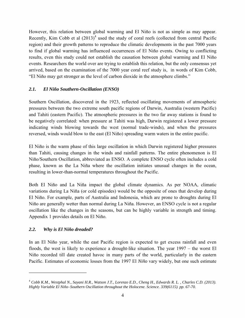
of fluctuations in the air pressure between the western and eastern tropical Pacific. Oceanic Niño Index (ONI) is used to measure the former and the Southern Oscillation Index (SOI) captures fluctuations in the latter. For other indicators used for monitoring ENSO events globally, the reader may refer to Appendix 2. The Oceanic Niño Index (ONI) is the standard measure used to monitor El Niño (La Niña) events. ONI is a Niño index based on ERSST (extended reconstruction sea surface temperature) data and is defined by sea-surface temperature anomalies6 (SSTA) of Niño 3.4 sea area.7 These temperature deviations/anomalies are captured as three months' moving averages in the Oceanic Niño Index (ONI). Twelve ONI values (Figure 1) are given for each year. An ONI anomaly (ONIA) value released in March of a year, for example, will be for Jan-Feb-Mar; the last month on the three-month average is considered the current month.

If for a year, five consecutive three-month moving average SST anomalies (for Niño 3.4 region) are greater (or lower than) than 0.5° C (-0.5° C)

8, then the year is classified as an El Niño (La 5 Climate Change Research Centre (2014). Get Used to Heat Waves: Extreme El Nino Events to Double. The

University of New South Wales. 6 NOAA defines an anomaly as variations from an average or other statistical reference value. In case of ONI, the

anomalies are calculated based on climatology between 1971 and 2000. 7 The Niño indices are calculated for four regions: 1+2, 3, 3.4 and 4. Niño 1+2 is an indicator for coastal El Niño,

which influences the coasts of Ecuador and northern Peru. Niño 3 is an indicator of variability in the cold tongue (left of Niño 1+2), whereas Niño 4 is on the edge of the warm pool in the ocean (left of the Niño3 ). These regions represent areas of the ocean, successively moving left wards. Niño 3.4 combines parts of both Niño 3 and Niño 4 regions, and is the best overall indicator of the strength of an El Niño(La Niña).

8 According to the Australian Bureau of Meteorology, the temperature threshold for El Niño is +0.8°C. We however, follow the NOAA threshold of +0.5°C.

6

Jan-Feb-Mar May-Jun-Jul

Jun-Jul-Aug

Mar-Apr-May

Feb-Mar-Apr

Jul-Aug-Sep

Oct-Nov-Dec

Nov-Dec-Jan Sep-Oct-Nov

Aug-Sep-Oct

Apr-May-Jun Dec-Jan-Feb

Niña) year. In terms of the absolute temperature of the sea-surface, this threshold of 0.5° C (-0.5° C) corresponds to an absolute sea-surface temperature reaching or exceeding (falling below) 28°

C (NOAA). Figure 1: The ONI-A values

The above temperature threshold can be further broken down into weak (when the anomaly is between 0.5 and 0.9° C), moderate (when between 1 and 1.4° C) and strong (when the anomaly is equal to or greater than 1.5° C) for El Niño events. The break down for La Niña can be similarly done. 2.5. El Niño Historical Trends

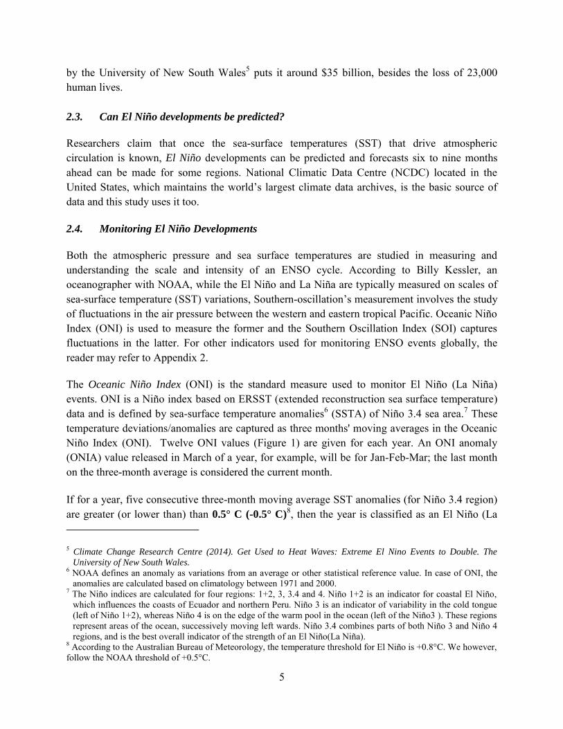
Based on the three threshold limits, we analysed the El Niño (La Niña) events since the 1950s (Figure 2). It shows that in these 64 years, there were 23 El Niño years and 22 La Niña years, and of these 22 per cent and 9 per cent were strong El Niño and La Niña years respectively. The average sea-surface temperature anomaly9 as captured under the ONIA for the 23 El Niño years was close to 1.2 °C, while that for the 22 La Niña years was -1.1 °C. The average ONIA values for the worst of the El Niño and La Niña episodes are given in the Appendix 2 for the interested reader.

Figure 2: La Niña and El Niña years since 1950

Source: NOAA

9 The value is calculated as the average of the 5-releavnt consecutive ONIA values (°Celsius), which are used to

measure El Niño/La Niña developments.

Indian Monsoon Rainfall Season- Jun-Sep

7

A decade-wise look at the climate anomalies shows that 7-8 years in every decade have witnessed either excessive warming (El Niño) or excessive cooling (La Niña). The decade of 1960s was the only exception where, even though there were four El Niño years, there was only one La Niña year, making the total of five years of aberrations. 3. Indian Droughts

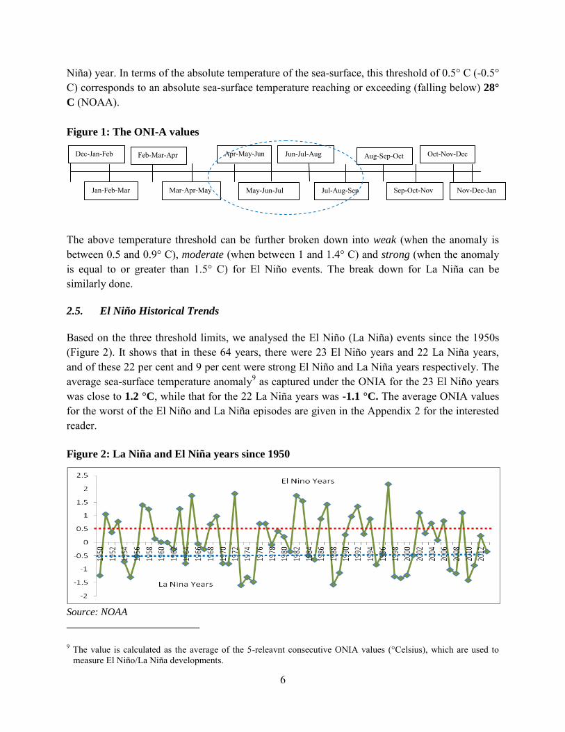
According to the Indian Meteorological Department (IMD), when the rainfall for the monsoon season of June to September for the country as a whole is within 10 per cent of its long period average (LPA), it is categorised as a normal monsoon but when the monsoon rainfall deficiency exceeds 10 per cent and affects more than 20 per cent of the country’s area, it is categorised as an all-India drought year. The LPA is the average or normal rainfall value calculated for all-India or for smaller areas based on an average of actual rainfall received between 1951 and 2000; all-India LPA for monsoon rains is 886.9 mm or say 89 cm. During 1901 to 2013, India faced 22 drought years: the worst was in 1918, when rainfall was 25 per cent below LPA; second worst in 1972 with rainfall deficiency of 23.9 per cent; and third worst was in 2009, when rainfall dipped 22 per cent below LPA (Figure 3). Figure 3: Indian Monsoons since 1901

Source: IMD

An analysis of 113 years of rainfall data does not suggest any systematic pattern in the occurrence of droughts. For example, there were two decades in the first half of the 20th century without any drought (1921/30 and 1931/40), but there was only one during 1991-2000; and three during 2001-2010. However, on an average, since 1901, droughts occurred, every five years and one month. This period reduces to four years and seven months when the data for the last 13 years (since 2001) is used, perhaps indicating an increased frequency of droughts.

8

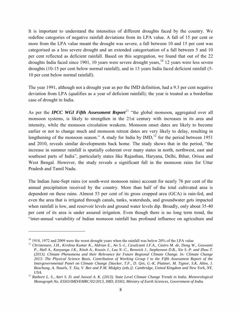
It is important to understand the intensities of different droughts faced by the country. We redefine categories of negative rainfall deviations from its LPA value. A fall of 15 per cent or more from the LPA value meant the drought was severe, a fall between 10 and 15 per cent was categorised as a less severe drought and an extended categorisation of a fall between 5 and 10 per cent reflected as deficient rainfall. Based on this segregation, we found that out of the 22 droughts India faced since 1901, 10 years were severe drought years,10 12 years were less severe droughts (10-15 per cent below normal rainfall), and in 13 years India faced deficient rainfall (5-10 per cent below normal rainfall). The year 1991, although not a drought year as per the IMD definition, had a 9.3 per cent negative deviation from LPA (qualifies as a year of deficient rainfall); the year is treated as a borderline case of drought in India. As per the IPCC WGI Fifth Assessment Report

11 “the global monsoon, aggregated over all monsoon systems, is likely to strengthen in the 21st century with increases in its area and intensity, while the monsoon circulation weakens. Monsoon onset dates are likely to become earlier or not to change much and monsoon retreat dates are very likely to delay, resulting in lengthening of the monsoon season.” A study for India by IMD,12 for the period between 1951 and 2010, reveals similar developments back home. The study shows that in the period, “the

increase in summer rainfall is spatially coherent over many states in north, northwest, east and southeast parts of India”, particularly states like Rajasthan, Haryana, Delhi, Bihar, Orissa and West Bengal. However, the study reveals a significant fall in the monsoon rains for Uttar Pradesh and Tamil Nadu. The Indian June-Sept rains (or south-west monsoon rains) account for nearly 76 per cent of the annual precipitation received by the country. More than half of the total cultivated area is dependent on these rains. Almost 53 per cent of its gross cropped area (GCA) is rain-fed, and even the area that is irrigated through canals, tanks, watersheds, and groundwater gets impacted when rainfall is low, and reservoir levels and ground water levels dip. Broadly, only about 35-40 per cent of its area is under assured irrigation. Even though there is no long term trend, the “inter-annual variability of Indian monsoon rainfall has profound influence on agriculture and

10 1918, 1972 and 2009 were the worst drought years when the rainfall was below 20% of the LPA value 11 Christensen, J.H., Krishna Kumar K., Aldrian E., An S.-I., Cavalcanti I.F.A., Castro M. de, Dong W., Goswami

P., Hall A., Kanyanga J.K., Kitoh A., Kossin J., Lau N.-C., Renwick J., Stephenson D.B., Xie S.-P. and Zhou T.

(2013). Climate Phenomena and their Relevance for Future Regional Climate Change. In: Climate Change

2013: The Physical Science Basis. Contribution of Working Group I to the Fifth Assessment Report of the

Intergovernmental Panel on Climate Change [Stocker, T.F., D. Qin, G.-K. Plattner, M. Tignor, S.K. Allen, J.

Boschung, A. Nauels, Y. Xia, V. Bex and P.M. Midgley (eds.)]. Cambridge, United Kingdom and New York, NY,

USA. 12 Rathore L. S., Attri S. D. and Jaswal A. K. (2013). State Level Climate Change Trends in India. Meteorological

Monograph No. ESSO/IMD/EMRC/02/2013, IMD, ESSO, Ministry of Earth Sciences, Government of India.

9

national economy (sic)” (IMD 2006 13). Econometric modelling shows that agriculture GDP, when calculated for a crop year (July-June) falls by about 0.35 per cent points with every 1 per cent point fall (from its long period average value) in monsoon rains (Gulati and Saini, 201314). Gadgil and Gadgil (2006) 15 found that deficient rainfall impacted the GDP and food grain production of the country more than surplus rainfall. While results from these studies are pivotal in understanding agriculture GDP’s vulnerability to

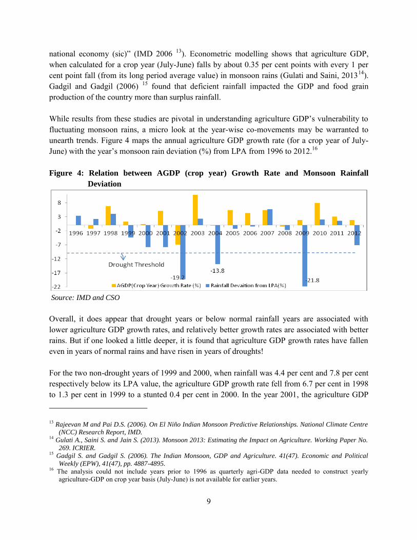
fluctuating monsoon rains, a micro look at the year-wise co-movements may be warranted to unearth trends. Figure 4 maps the annual agriculture GDP growth rate (for a crop year of July-June) with the year’s monsoon rain deviation (%) from LPA from 1996 to 2012.16 Figure 4: Relation between AGDP (crop year) Growth Rate and Monsoon Rainfall

Deviation

Source: IMD and CSO

Overall, it does appear that drought years or below normal rainfall years are associated with lower agriculture GDP growth rates, and relatively better growth rates are associated with better rains. But if one looked a little deeper, it is found that agriculture GDP growth rates have fallen even in years of normal rains and have risen in years of droughts! For the two non-drought years of 1999 and 2000, when rainfall was 4.4 per cent and 7.8 per cent respectively below its LPA value, the agriculture GDP growth rate fell from 6.7 per cent in 1998 to 1.3 per cent in 1999 to a stunted 0.4 per cent in 2000. In the year 2001, the agriculture GDP 13 Rajeevan M and Pai D.S. (2006). On El Niño Indian Monsoon Predictive Relationships. National Climate Centre

(NCC) Research Report, IMD. 14 Gulati A., Saini S. and Jain S. (2013). Monsoon 2013: Estimating the Impact on Agriculture. Working Paper No.

269. ICRIER. 15 Gadgil S. and Gadgil S. (2006). The Indian Monsoon, GDP and Agriculture. 41(47). Economic and Political

Weekly (EPW), 41(47), pp. 4887-4895. 16 The analysis could not include years prior to 1996 as quarterly agri-GDP data needed to construct yearly

agriculture-GDP on crop year basis (July-June) is not available for earlier years.

10

growth was commendable at 5.1 per cent with a close to 8 per cent negative deviation in rainfall from its LPA value. In 2009, the third worst drought faced by India in the last 113 years, India’s

agriculture GDP grew close to 2 per cent! Does it indicate a growing resilience of Indian agriculture to droughts? It is too early to say this with limited observations, but the emerging trends perhaps do point towards that. Increasing irrigation coverage, mainly through the spurt in ground water usage (Gulati and Saini 2013) could be behind such a trend. Data from the Ministry of Agriculture indicate that close to 60 per cent of irrigation was through canals (private and government) and tanks and less than 30 per cent was through ground water sources in the 1950s. The decade of the 2000s saw these roles reversed. Close to 62 per cent of the total irrigation in 2009 was through tube wells and wells and less than 30 per cent was from canals and tanks. Among other factors, this trend also contributed to expanding the irrigation coverage through the country. This would have contributed in reducing the agriculture sector’s

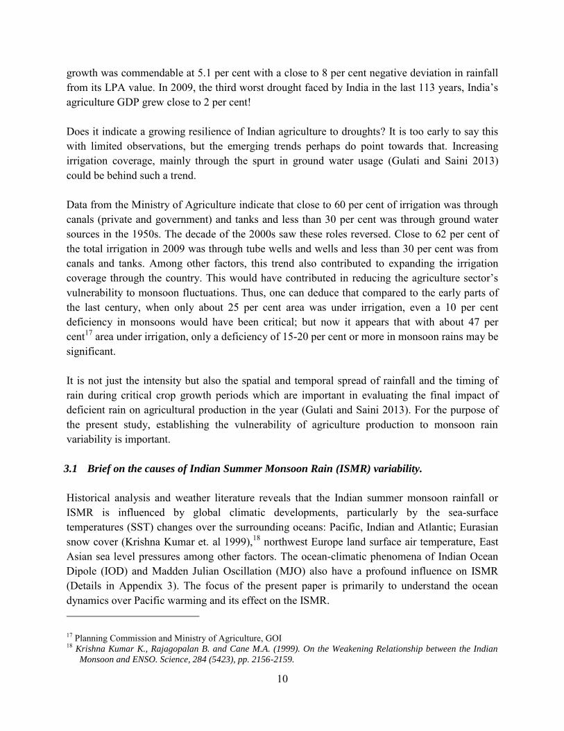
vulnerability to monsoon fluctuations. Thus, one can deduce that compared to the early parts of the last century, when only about 25 per cent area was under irrigation, even a 10 per cent deficiency in monsoons would have been critical; but now it appears that with about 47 per cent17 area under irrigation, only a deficiency of 15-20 per cent or more in monsoon rains may be significant. It is not just the intensity but also the spatial and temporal spread of rainfall and the timing of rain during critical crop growth periods which are important in evaluating the final impact of deficient rain on agricultural production in the year (Gulati and Saini 2013). For the purpose of the present study, establishing the vulnerability of agriculture production to monsoon rain variability is important. 3.1 Brief on the causes of Indian Summer Monsoon Rain (ISMR) variability.

Historical analysis and weather literature reveals that the Indian summer monsoon rainfall or ISMR is influenced by global climatic developments, particularly by the sea-surface temperatures (SST) changes over the surrounding oceans: Pacific, Indian and Atlantic; Eurasian snow cover (Krishna Kumar et. al 1999),18 northwest Europe land surface air temperature, East Asian sea level pressures among other factors. The ocean-climatic phenomena of Indian Ocean Dipole (IOD) and Madden Julian Oscillation (MJO) also have a profound influence on ISMR (Details in Appendix 3). The focus of the present paper is primarily to understand the ocean dynamics over Pacific warming and its effect on the ISMR. 17 Planning Commission and Ministry of Agriculture, GOI 18 Krishna Kumar K., Rajagopalan B. and Cane M.A. (1999). On the Weakening Relationship between the Indian

Monsoon and ENSO. Science, 284 (5423), pp. 2156-2159.

11

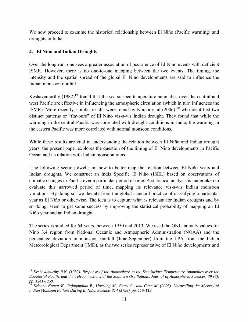
We now proceed to examine the historical relationship between El Niño (Pacific warming) and droughts in India. 4. El Niño and Indian Droughts

Over the long run, one sees a greater association of occurrence of El Niño events with deficient ISMR. However, there is no one-to-one mapping between the two events. The timing, the intensity and the spatial spread of the global El Niño developments are said to influence the Indian monsoon rainfall. Keshavamurthy (1982)19 found that the sea-surface temperature anomalies over the central and west Pacific are effective in influencing the atmospheric circulation (which in turn influences the ISMR). More recently, similar results were found by Kumar et.al (2006),20 who identified two distinct patterns or “flavours” of El Niño vis-à-vis Indian drought. They found that while the warming in the central Pacific was correlated with drought conditions in India, the warming in the eastern Pacific was more correlated with normal monsoon conditions. While these results are vital in understanding the relation between El Niño and Indian drought years, the present paper explores the question of the timing of El Niño developments in Pacific Ocean and its relation with Indian monsoon rains. The following section dwells on how to better map the relation between El Niño years and Indian droughts. We construct an India Specific El Niño (ISEL) based on observations of climatic changes in Pacific over a particular period of time. A statistical analysis is undertaken to evaluate this narrowed period of time, mapping its relevance vis-à-vis Indian monsoon variations. By doing so, we deviate from the global standard practice of classifying a particular year as El Niño or otherwise. The idea is to capture what is relevant for Indian droughts and by so doing, seem to get some success by improving the statistical probability of mapping an El Niño year and an Indian drought. The series is studied for 64 years, between 1950 and 2013. We used the ONI anomaly values for Niño 3.4 region from National Oceanic and Atmospheric Administration (NOAA) and the percentage deviation in monsoon rainfall (June-September) from the LPA from the Indian Meteorological Department (IMD), as the two series representative of El Niño developments and

19 Keshavamurthy R.N. (1982). Response of the Atmosphere to the Sea Surface Temperature Anomalies over the

Equatorial Pacific and the Teleconnections of the Southern Oscillations, Journal of Atmospheric Sciences, 39 (6),

pp. 1241-1259. 20 Krishna Kumar K., Rajagopalan B., Hoerling M., Bates G., and Cane M. (2006). Unravelling the Mystery of

Indian Monsoon Failure During El Niño. Science. 314 (5796). pp. 115-118.

12

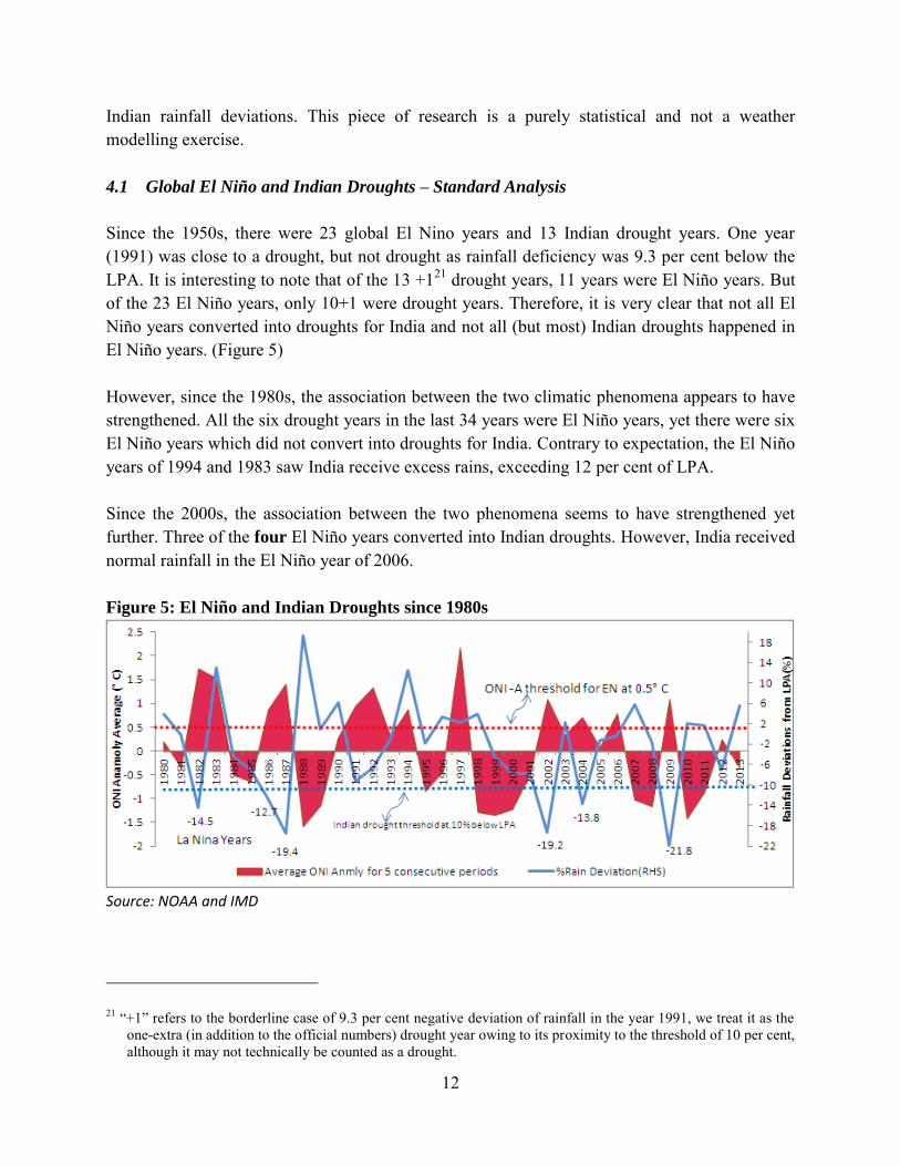
Indian rainfall deviations. This piece of research is a purely statistical and not a weather modelling exercise. 4.1 Global El Niño and Indian Droughts – Standard Analysis

Since the 1950s, there were 23 global El Nino years and 13 Indian drought years. One year (1991) was close to a drought, but not drought as rainfall deficiency was 9.3 per cent below the LPA. It is interesting to note that of the 13 +121 drought years, 11 years were El Niño years. But of the 23 El Niño years, only 10+1 were drought years. Therefore, it is very clear that not all El Niño years converted into droughts for India and not all (but most) Indian droughts happened in El Niño years. (Figure 5) However, since the 1980s, the association between the two climatic phenomena appears to have strengthened. All the six drought years in the last 34 years were El Niño years, yet there were six El Niño years which did not convert into droughts for India. Contrary to expectation, the El Niño years of 1994 and 1983 saw India receive excess rains, exceeding 12 per cent of LPA. Since the 2000s, the association between the two phenomena seems to have strengthened yet further. Three of the four El Niño years converted into Indian droughts. However, India received normal rainfall in the El Niño year of 2006. Figure 5: El Niño and Indian Droughts since 1980s

Source: NOAA and IMD

21 “+1” refers to the borderline case of 9.3 per cent negative deviation of rainfall in the year 1991, we treat it as the

one-extra (in addition to the official numbers) drought year owing to its proximity to the threshold of 10 per cent, although it may not technically be counted as a drought.

13

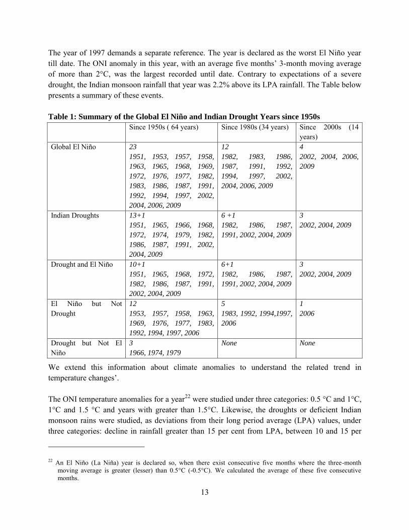
The year of 1997 demands a separate reference. The year is declared as the worst El Niño year till date. The ONI anomaly in this year, with an average five months’ 3-month moving average of more than 2°C, was the largest recorded until date. Contrary to expectations of a severe drought, the Indian monsoon rainfall that year was 2.2% above its LPA rainfall. The Table below presents a summary of these events. Table 1: Summary of the Global El Niño and Indian Drought Years since 1950s

Since 1950s ( 64 years) Since 1980s (34 years) Since 2000s (14 years)

Global El Niño 23

1951, 1953, 1957, 1958,

1963, 1965, 1968, 1969,

1972, 1976, 1977, 1982,

1983, 1986, 1987, 1991,

1992, 1994, 1997, 2002,

2004, 2006, 2009

12

1982, 1983, 1986,

1987, 1991, 1992,

1994, 1997, 2002,

2004, 2006, 2009

4

2002, 2004, 2006,

2009

Indian Droughts 13+1

1951, 1965, 1966, 1968,

1972, 1974, 1979, 1982,

1986, 1987, 1991, 2002,

2004, 2009

6 +1

1982, 1986, 1987,

1991, 2002, 2004, 2009

3

2002, 2004, 2009

Drought and El Niño 10+1

1951, 1965, 1968, 1972,

1982, 1986, 1987, 1991,

2002, 2004, 2009

6+1

1982, 1986, 1987,

1991, 2002, 2004, 2009

3

2002, 2004, 2009

El Niño but Not Drought

12

1953, 1957, 1958, 1963,

1969, 1976, 1977, 1983,

1992, 1994, 1997, 2006

5

1983, 1992, 1994,1997,

2006

1

2006

Drought but Not El Niño

3

1966, 1974, 1979

None None

We extend this information about climate anomalies to understand the related trend in temperature changes’. The ONI temperature anomalies for a year22 were studied under three categories: 0.5 °C and 1°C, 1°C and 1.5 °C and years with greater than 1.5°C. Likewise, the droughts or deficient Indian monsoon rains were studied, as deviations from their long period average (LPA) values, under three categories: decline in rainfall greater than 15 per cent from LPA, between 10 and 15 per

22 An El Niño (La Niña) year is declared so, when there exist consecutive five months where the three-month

moving average is greater (lesser) than 0.5°C (-0.5°C). We calculated the average of these five consecutive months.

14

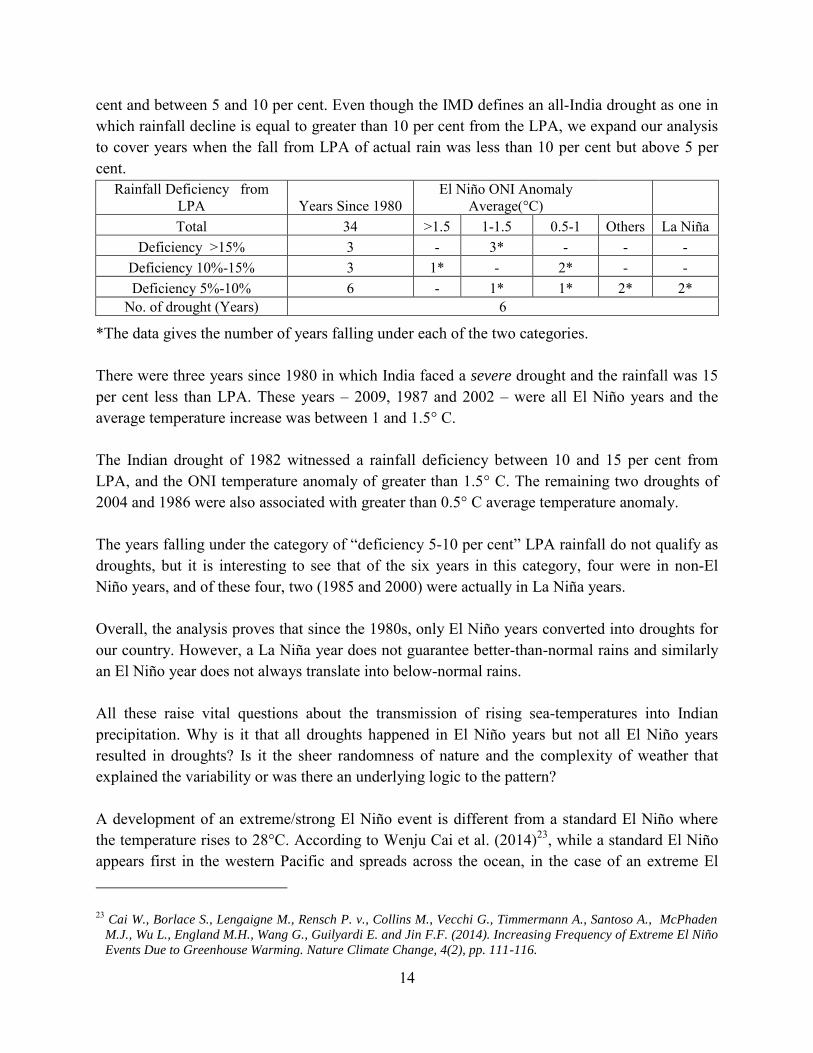
cent and between 5 and 10 per cent. Even though the IMD defines an all-India drought as one in which rainfall decline is equal to greater than 10 per cent from the LPA, we expand our analysis to cover years when the fall from LPA of actual rain was less than 10 per cent but above 5 per cent.

Rainfall Deficiency from LPA Years Since 1980

El Niño ONI Anomaly Average(°C)

Total 34 >1.5 1-1.5 0.5-1 Others La Niña Deficiency >15% 3 - 3* - - -

Deficiency 10%-15% 3 1* - 2* - - Deficiency 5%-10% 6 - 1* 1* 2* 2*

No. of drought (Years) 6

*The data gives the number of years falling under each of the two categories. There were three years since 1980 in which India faced a severe drought and the rainfall was 15 per cent less than LPA. These years – 2009, 1987 and 2002 – were all El Niño years and the average temperature increase was between 1 and 1.5° C. The Indian drought of 1982 witnessed a rainfall deficiency between 10 and 15 per cent from LPA, and the ONI temperature anomaly of greater than 1.5° C. The remaining two droughts of 2004 and 1986 were also associated with greater than 0.5° C average temperature anomaly. The years falling under the category of “deficiency 5-10 per cent” LPA rainfall do not qualify as droughts, but it is interesting to see that of the six years in this category, four were in non-El Niño years, and of these four, two (1985 and 2000) were actually in La Niña years. Overall, the analysis proves that since the 1980s, only El Niño years converted into droughts for our country. However, a La Niña year does not guarantee better-than-normal rains and similarly an El Niño year does not always translate into below-normal rains. All these raise vital questions about the transmission of rising sea-temperatures into Indian precipitation. Why is it that all droughts happened in El Niño years but not all El Niño years resulted in droughts? Is it the sheer randomness of nature and the complexity of weather that explained the variability or was there an underlying logic to the pattern? A development of an extreme/strong El Niño event is different from a standard El Niño where the temperature rises to 28°C. According to Wenju Cai et al. (2014)23, while a standard El Niño appears first in the western Pacific and spreads across the ocean, in the case of an extreme El 23 Cai W., Borlace S., Lengaigne M., Rensch P. v., Collins M., Vecchi G., Timmermann A., Santoso A., McPhaden

M.J., Wu L., England M.H., Wang G., Guilyardi E. and Jin F.F. (2014). Increasing Frequency of Extreme El Niño

Events Due to Greenhouse Warming. Nature Climate Change, 4(2), pp. 111-116.

15

Niño, SSTs rise above 28°C in the normally cold and dry eastern equatorial Pacific Ocean first. In the case of India, research by Krishna et al. (2007), as mentioned before, found that warming in the central Pacific was correlated with drought conditions in India, and the warming in the eastern Pacific was more correlated with normal monsoon conditions. This highlights the varying impact on ISMR with varying spatial developments of El Niño. Apart from such spatial differences, even the timing and the intensity of such developments make a difference to their impact on the Indian summer monsoon rains (ISMR). The next sub-section explores independently, the mapping of the timing of the El Niño developments together with the ISMR variations. 4.2 Constructing an India Specific El Niño (ISEL) to Map Indian Droughts

The key challenge for an Indian weather scientist and a policy maker is to find out when an El Niño can turn into a severe drought in India. Motivated by the weak relation and sometimes the disconnect between El Niño developments globally and Indian droughts, the study undertakes a statistical analysis to evaluate a narrowed period of time, by mapping the El Niño developments with Indian summer monsoon rainfall (ISMR) variations. With this motivation, we went back to the definition of El Niño. As mentioned before, an El Niño, measured by ONI, referred to a situation when five consecutive three-month moving average ONIA values exceeded 0.5°C. Now, we found that these five consecutive readings did not follow a pattern across years; sometimes these five readings were in the early part of the year and sometimes in the middle and sometimes in the latter part of the year. For example, in the year 1983, these five consecutive months started in January, while for 1986, it only got highlighted in September. Our hypothesis was that for any year, not all the 12 readings of ONIA would be of importance to our June to September monsoon rains. In particular, it was felt that the three-monthly-moving-averages, especially say from October-November-December to Feb-March-April, may not have much impact on ISMR. This is supported by our statistical analysis. After analysing averages of various combinations of the 12 ONIA readings, together with Indian monsoon variations, we found that the average of the ONI values from April-May-June to September-October-November (AMJ-SON) emerged most relevant24

in explaining Indian monsoon variations.

24 Relevance was defined as the capability of a combination of ONIA values in explaining the variability in Indian

monsoons. So, if for a narrowed period values of ONIA in a year, the average implied El Niño developments and the Indian monsoon rains did experience drought in that year, then the mapping between the El Niño developments globally and Indian drought was found to be perfect/relevant.

16

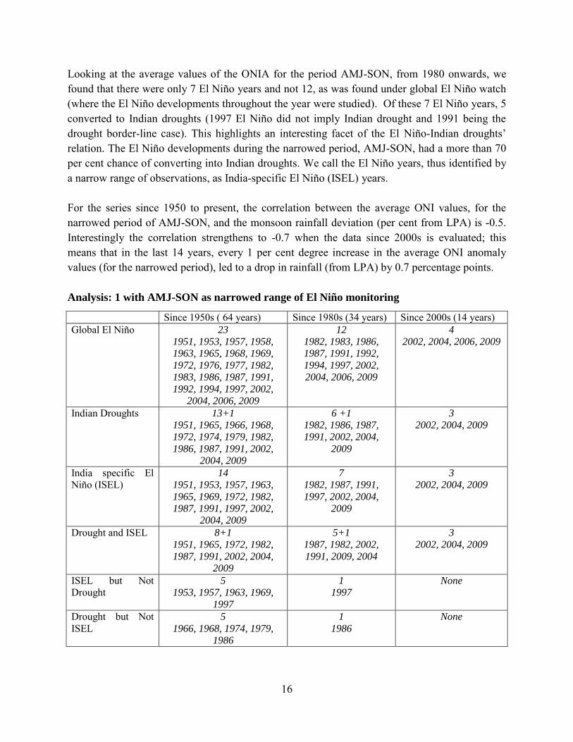
Looking at the average values of the ONIA for the period AMJ-SON, from 1980 onwards, we found that there were only 7 El Niño years and not 12, as was found under global El Niño watch (where the El Niño developments throughout the year were studied). Of these 7 El Niño years, 5 converted to Indian droughts (1997 El Niño did not imply Indian drought and 1991 being the drought border-line case). This highlights an interesting facet of the El Niño-Indian droughts’

relation. The El Niño developments during the narrowed period, AMJ-SON, had a more than 70 per cent chance of converting into Indian droughts. We call the El Niño years, thus identified by a narrow range of observations, as India-specific El Niño (ISEL) years. For the series since 1950 to present, the correlation between the average ONI values, for the narrowed period of AMJ-SON, and the monsoon rainfall deviation (per cent from LPA) is -0.5. Interestingly the correlation strengthens to -0.7 when the data since 2000s is evaluated; this means that in the last 14 years, every 1 per cent degree increase in the average ONI anomaly values (for the narrowed period), led to a drop in rainfall (from LPA) by 0.7 percentage points. Analysis: 1 with AMJ-SON as narrowed range of El Niño monitoring

Since 1950s ( 64 years) Since 1980s (34 years) Since 2000s (14 years) Global El Niño 23

1951, 1953, 1957, 1958,

1963, 1965, 1968, 1969,

1972, 1976, 1977, 1982,

1983, 1986, 1987, 1991,

1992, 1994, 1997, 2002,

2004, 2006, 2009

12

1982, 1983, 1986,

1987, 1991, 1992,

1994, 1997, 2002,

2004, 2006, 2009

4

2002, 2004, 2006, 2009

Indian Droughts 13+1

1951, 1965, 1966, 1968,

1972, 1974, 1979, 1982,

1986, 1987, 1991, 2002,

2004, 2009

6 +1

1982, 1986, 1987,

1991, 2002, 2004,

2009

3

2002, 2004, 2009

India specific El Niño (ISEL)

14

1951, 1953, 1957, 1963,

1965, 1969, 1972, 1982,

1987, 1991, 1997, 2002,

2004, 2009

7

1982, 1987, 1991,

1997, 2002, 2004,

2009

3

2002, 2004, 2009

Drought and ISEL 8+1

1951, 1965, 1972, 1982,

1987, 1991, 2002, 2004,

2009

5+1

1987, 1982, 2002,

1991, 2009, 2004

3

2002, 2004, 2009

ISEL but Not Drought

5

1953, 1957, 1963, 1969,

1997

1

1997

None

Drought but Not ISEL

5

1966, 1968, 1974, 1979,

1986

1

1986

None

17

Looking at the last 14 years, there appeared four El Niño years globally but only three appeared as per our ISEL calculations. All these three ISELs resulted in Indian droughts. Although such a narrowed mapping of ISELs increases our chances of understanding the co-movements of ONI developments globally with domestic monsoon variations, it also runs the risk of missing out a 1986 El Niño and drought, when sea temperature warming was visible only after September of the year. There is also a risk of over-inclusion as for instance happened in the case of the year 1997, the worst El Niño year till date, when India had healthy rainfall but it nevertheless, got included under ISEL calculations. Still, as highlighted above, there does not appear any one-to-one correspondence between the two phenomenon. Nevertheless, when one looked at comparatively shorter period values of ONI changes, the chances of understanding and predicting an ISEL development appear to increase. Since these ISEL developments are tracked simultaneously through the months of the ISMR, the use of this method and this period towards predicting an Indian drought in the year under consideration may not be useful. But for undertaking an ex-post analysis of the likely relation between El Niño global developments and the ISMR variations, this method may be useful. 5. Preparing for Exigency: If 2014 turns out to be an El Niño and a drought in India

Scientists the world over are seeing increased evidence of an upcoming change in the Pacific Ocean’s sub-surface, which favours the development of a moderate-to-strong El Niño event in the spring/summer of 2014. There are four ONI anomaly values for 2014 yet and all are still in negatives, reflecting thus the lower-than-average temperatures in the Ocean. However, these values are successively falling, indicating a rise in sea-temperatures. These values are -0.6 for DJF, -0.6 for JFM, -0.5 for FMA and -0.2 for MAM. What explains the increased apprehensions about El Niño in 2014? The answer lies in ocean-climate dynamics captured beyond the ONI- anomaly indicator. There are several types of waves in the Pacific Ocean, and one such wave is called “Oceanic

Kelvin wave”, which gains momentum from wind bursts in the West Pacific region heading east. The Super El Niño of 1997 (the worst El Niño till date) was born out of this oceanic Kelvin wave event. However, this wave was not the only reason for the El Niño in 1997, when the wave dynamics initiated by the Kelvin wave were intensified by complementing cyclones during the time. Since middle of 2013, there have been a series of strong Kelvin waves, resulting in massive warming below the sea-surface.

18

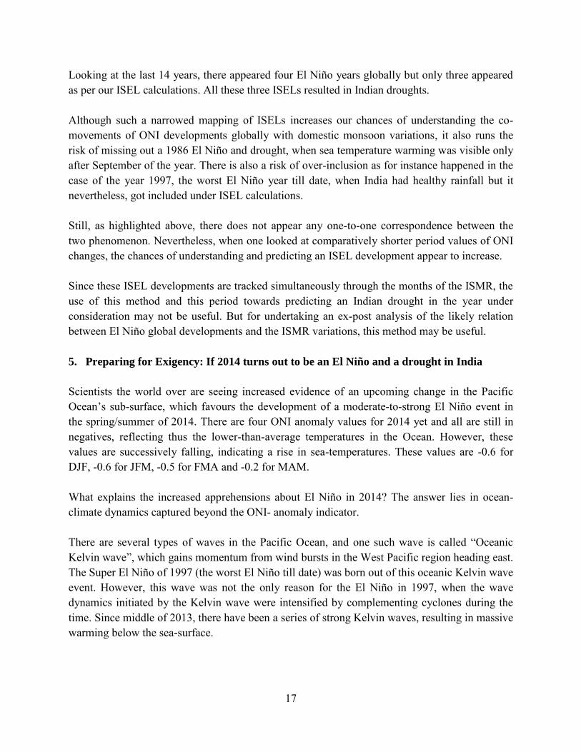
Figure 6: Sea-surface Temperatures

Week Centred on 04 June 2014

Source: NOAA

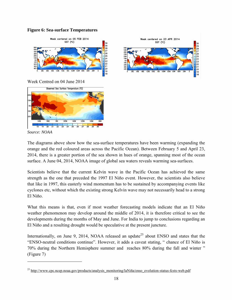
The diagrams above show how the sea-surface temperatures have been warming (expanding the orange and the red coloured areas across the Pacific Ocean). Between February 5 and April 23, 2014, there is a greater portion of the sea shown in hues of orange, spanning most of the ocean surface. A June 04, 2014, NOAA image of global sea waters reveals warming sea-surfaces. Scientists believe that the current Kelvin wave in the Pacific Ocean has achieved the same strength as the one that preceded the 1997 El Niño event. However, the scientists also believe that like in 1997, this easterly wind momentum has to be sustained by accompanying events like cyclones etc, without which the existing strong Kelvin wave may not necessarily head to a strong El Niño. What this means is that, even if most weather forecasting models indicate that an El Niño weather phenomenon may develop around the middle of 2014, it is therefore critical to see the developments during the months of May and June. For India to jump to conclusions regarding an El Niño and a resulting drought would be speculative at the present juncture. Internationally, on June 9, 2014, NOAA released an update25 about ENSO and states that the “ENSO-neutral conditions continue”. However, it adds a caveat stating, “ chance of El Niño is 70% during the Northern Hemisphere summer and reaches 80% during the fall and winter ” (Figure 7) 25 http://www.cpc.ncep.noaa.gov/products/analysis_monitoring/laNiña/enso_evolution-status-fcsts-web.pdf

19

Figure 7: Climate Prediction Centre’s ENSO forecast

Source: NOAA

As a result of these global developments, monsoon predictions have achieved a new importance for setting into motion timely and effective preparedness and mitigation activities. There have been two forecasts about the 2014 monsoon rains in India – one by the Indian Meteorological Department (IMD) and one by a private weather monitoring firm, Skymet. The IMD’s second stage long-range forecast for the 2014 southwest monsoon season rainfall, released on June 09, 2014,26 predicts that rains in the season will be 93 per cent of the long period average (LPA of 890 mm) with an error of + 4 per cent. IMD acknowledges the 70 per cent chances of El Niño warming reaching its peak during the south-west monsoon season. The release pegs the forecast probability of 2014 monsoon rainfall falling below normal at 38% and deficient at 33 per cent. This indicates 71 per cent likelihood of ISMR being deficient or below normal. (Appendix 4 outlines a brief of the forecast IMD method). Skymet, a private weather monitoring firm based in India, pegs the probabilities of below normal rainfall at 40 per cent and deficient rainfall at 25 per cent at 65 per cent. Comparison between the two forecasts is given below:

26 http://www.imd.gov.in/section/nhac/dynamic/2lrf_eng14.pdf . Accessed on June 11, 2014.

20

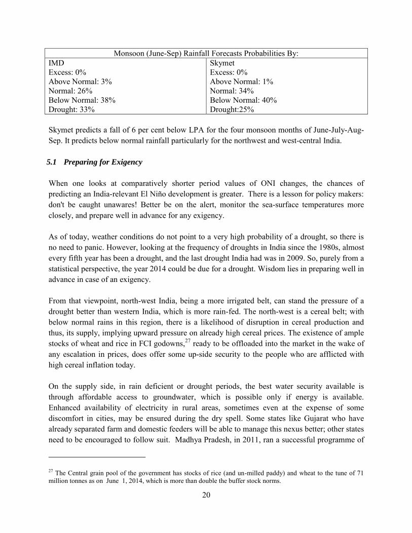
Monsoon (June-Sep) Rainfall Forecasts Probabilities By: IMD Excess: 0% Above Normal: 3% Normal: 26% Below Normal: 38% Drought: 33%

Skymet Excess: 0% Above Normal: 1% Normal: 34% Below Normal: 40% Drought:25%

Skymet predicts a fall of 6 per cent below LPA for the four monsoon months of June-July-Aug-Sep. It predicts below normal rainfall particularly for the northwest and west-central India. 5.1 Preparing for Exigency

When one looks at comparatively shorter period values of ONI changes, the chances of predicting an India-relevant El Niño development is greater. There is a lesson for policy makers: don't be caught unawares! Better be on the alert, monitor the sea-surface temperatures more closely, and prepare well in advance for any exigency. As of today, weather conditions do not point to a very high probability of a drought, so there is no need to panic. However, looking at the frequency of droughts in India since the 1980s, almost every fifth year has been a drought, and the last drought India had was in 2009. So, purely from a statistical perspective, the year 2014 could be due for a drought. Wisdom lies in preparing well in advance in case of an exigency. From that viewpoint, north-west India, being a more irrigated belt, can stand the pressure of a drought better than western India, which is more rain-fed. The north-west is a cereal belt; with below normal rains in this region, there is a likelihood of disruption in cereal production and thus, its supply, implying upward pressure on already high cereal prices. The existence of ample stocks of wheat and rice in FCI godowns,27 ready to be offloaded into the market in the wake of any escalation in prices, does offer some up-side security to the people who are afflicted with high cereal inflation today. On the supply side, in rain deficient or drought periods, the best water security available is through affordable access to groundwater, which is possible only if energy is available. Enhanced availability of electricity in rural areas, sometimes even at the expense of some discomfort in cities, may be ensured during the dry spell. Some states like Gujarat who have already separated farm and domestic feeders will be able to manage this nexus better; other states need to be encouraged to follow suit. Madhya Pradesh, in 2011, ran a successful programme of

27 The Central grain pool of the government has stocks of rice (and un-milled paddy) and wheat to the tune of 71 million tonnes as on June 1, 2014, which is more than double the buffer stock norms.

21

providing its farmers 1 million temporary power connections, during their heavy-demand, rabi crop season This program could be extended in case of a drought to its kharif crops like soybean, which are largely rain-fed. Poor farmers who depend on diesel pumps to meet their small irrigation needs may be suitably compensated through diesel vouchers or other incentives to keep the cost of irrigation under control. In the long run, government supported, but privately managed, community tube wells operated through pre-paid smart cards (as in the Barind tract in Bangladesh) may be established to enhance water access and security of small and distressed farmers. These also provide these farmers a respite from the exploitation at the hands of large farmers in the oligopolistic groundwater markets. Western India is also a supplier of oilseeds, pulses, and cotton and thus, there could be pressures on their prices too. The fact that edible oils are largely imported from Indonesia and Malaysia, the South-East Asian countries, which, like India, may be equally affected by the El Niño, is a cause for concern. Analysis by the International Water Management Institute and Central Institute for Dryland Agriculture (Sharma et al., 2010) has shown that actually it is a small subset of the total number of rain-fed districts which grow most (> 85 per cent) of the soybean (21 districts), sunflower (11 districts), pigeon pea (85 districts), cotton (30 districts) and groundnut (50 districts) during the kharif season. Special attention to these districts will help maintain productivity and contain distress. A single supplemental irrigation to these crops even during drought years has the potential to enhance productivity by more than 50 per cent. A comfortable water position in the country’s reservoirs also offers a hedge for rain-fed areas. As on June 8, 2014, the live storage in the country’s 85 important reservoirs was “133 per cent of the storage of corresponding period of last year and 157 per cent of storage of average of last ten years. The present storage position during current year is better than storage position of last year and average storage of last ten years” (CWC).28 In particular, the states of Himachal Pradesh, Punjab, Rajasthan, Odisha, Gujarat, Maharashtra, Uttar Pradesh, Uttarakhand, Madhya Pradesh, Chhattisgarh, Karnataka, Kerala, and Tamil Nadu have a better storage position today than they did in the corresponding period last year. Going forward, there is an urgent need to expand insurance cover for farmers, or have an insurance/income stabilisation fund (say of Rs.5000 crore) to take care of any exigency. This can be done in the short run. Further, in the short run, cutting down import duties on fruits and vegetables, skimmed milk powder (SMP), chicken legs etc, to say 15 percent or so from their current levels would help in taming potential increase in food prices, in case of a sub-normal rainfall. The current duty structure for these commodities is generally above 30 percent, and in some cases, as in SMP it is 60% (beyond the in-quota tariff) and for chicken legs 100%.

28 Central Water Commission, Ministry of Water Resources, Accessed on June 8, 2014.

22

Over a longer period, however, India will have to invest heavily in the water sector, both on the supply side as well on better demand management, with more innovative policies, technology and products. And also, building effective value chains for perishable and high value agri-products like fruits and vegetables, eggs, fish and meat, milk and milk products, will help in containing food prices. In the 2014-15 central budget, the centre’s outlay for Mahatma Gandhi National Rural Employment Guarantee Scheme (MNREGS) is Rs.34,000 crore; the non-plan expenditure on fertiliser subsidy is close to Rs.68,000 crore (the Fertiliser Association of India (FAI) and fertiliser ministry estimates show that there still would exist pending bills of roughly Rs.35,000-40,000 crore) and on food subsidy, non-plan expenditure is pegged at a whooping Rs.1,15,000 crore (estimates reveal an additional need of Rs.40,000 to 50,000 crore in case of National Food Security Act is implemented). Compare this to the total expenditure of Rs.13,093 crore on water resources scheduled for the current fiscal. According to the 12th Plan document, there are 337 major, medium and other irrigation projects pending in India and an indicative outlay for the water resources sector, under the 12th Plan is stated to be about Rs.4,22,012 crore as against the central outlay of Rs.18,118 crore for FY14. Based on information from the Central Ground Water Board, the Planning Commission, in same document, says that more than 30 per cent of the area in India falls in the extreme water scarce zone, with less than 500 m3/person/year supply of renewable fresh water. In the last decade, the report claims that the country’s ground water level has been declining

annually by 4 cm. The present state of policy direction in the economy thus requires major reorientation. Instead of multiplying subsidies, greater investments are required in fields, which have the capability to augment supply of agriculture products. This will help in developing the long-term resilience of Indian agriculture, raise productivity and overall production. Similarly, the MGNREGA resources can be reoriented towards creating a massive programme for “watershed restoration and ground water recharge” (Planning Commission).29 The launch of “centrally sponsored scheme on micro irrigation” in January 2006 was a right step in this regard.

The scheme is part of the National Mission for Sustainable Agriculture (NMSA) adopted by the government, which has derived its mandate from National Action on Climate Change (NAPCC, 2008) and primarily focuses on synergising resource conservation, improved farm practices and integrated farming for “enhancing agricultural productivity especially in rain-fed areas”. While these mark the right intention of the government, synergising resources and efforts across related ministries remains an insurmountable challenge for the central government.

29 Planning Commission. (2013). 12th Five Year Plan, Chapter 5: Water, Volume I.

23

References

Cai W., Borlace S., Lengaigne M., Rensch P. v., Collins M., Vecchi G., Timmermann A.,

Santoso A., McPhaden M.J., Wu L., England M.H., Wang G., Guilyardi E. and Jin F.F.

(2014). Increasing Frequency of Extreme El Niño Events Due to Greenhouse Warming. Nature Climate Change, 4(2), pp. 111-116. Christensen, J.H., Krishna Kumar K., Aldrian E., An S.-I., Cavalcanti I.F.A., Castro M.

de, Dong W., Goswami P., Hall A., Kanyanga J.K., Kitoh A., Kossin J., Lau N.-C., Renwick

J., Stephenson D.B., Xie S.-P. and Zhou T. (2013). Climate Phenomena and their Relevance for Future Regional Climate Change. In: Climate Change 2013: The Physical Science Basis. Contribution of Working Group I to the Fifth Assessment Report of the Intergovernmental Panel on Climate Change [Stocker, T.F., D. Qin, G.-K. Plattner, M. Tignor, S.K. Allen, J. Boschung, A. Nauels, Y. Xia, V. Bex and P.M. Midgley (eds.)]. Cambridge, United Kingdom and New York, NY, USA. Climate Change Research Centre (2014). Get Used to Heat Waves: Extreme El Nino Events to Double. The University of New South Wales. Cobb K.M., Westphal N., Sayani H.R., Watson J.T., Lorenzo E.D., Cheng H., Edwards R.

L. , Charles C.D. (2013). Highly Variable El Niño–Southern Oscillation throughout the Holocene. Science. 339(6115). pp. 67-70. Fiondella F. (2009). Top Misconceptions about El Niño and La Niña. The Earth Institute, Columbia University. Gadgil S. and Gadgil S. (2006). The Indian Monsoon, GDP and Agriculture. 41(47). Economic and Political Weekly (EPW), 41(47), pp. 4887-4895. Gulati A., Saini S. and Jain S. (2013). Monsoon 2013: Estimating the Impact on Agriculture. Working Paper No. 269. ICRIER. Keshavamurthy R.N. (1982). Response of the Atmosphere to the Sea Surface Temperature Anomalies over the Equatorial Pacific and the Teleconnections of the Southern Oscillations, Journal of Atmospheric Sciences, 39 (6), pp. 1241-1259. Kessler B. FAQs, http://faculty.washington.edu/kessler/. Accessed May, 2014. Krishna Kumar K., Rajagopalan B. and Cane M.A. (1999). On the Weakening Relationship between the Indian Monsoon and ENSO. Science, 284 (5423), pp. 2156-2159.

24

Krishna Kumar K., Rajagopalan B., Hoerling M., Bates G., and Cane M. (2006). Unravelling the Mystery of Indian Monsoon Failure During El Niño. Science. 314 (5796). pp. 115-118. Planning Commission. (2013). 12th Five Year Plan, Chapter 5: Water, Volume I. Rajeevan M and Pai D.S. (2006). On El Niño Indian Monsoon Predictive Relationships. National Climate Centre (NCC) Research Report, IMD. Rathore L. S., Attri S. D. and Jaswal A. K. (2013). State Level Climate Change Trends in India. Meteorological Monograph No. ESSO/IMD/EMRC/02/2013, IMD, ESSO, Ministry of Earth Sciences, Government of India. Tisdale Bob - Climate Observations. (2010). The Multivariate ENSO Index (MEI) Captures the Global Temperature Impacts of ENSO Differently than SST-Based Indices. Trenberth K. E. and Timothy J H. (1996). The 1990–1995 El Niño-Southern Oscillation Event: Longest on Record. Geophysical Research Letters, 23 (1). pp. 57–60. Data Sources

Australian Bureau of Meteorology

Central Water Commission, Ministry of Water Resources, Accessed on June 8,2014

Directorate of Economics and Statistics, Ministry of Agriculture

Earth System Research Laboratory, Physical Science Division, National Oceanic and

Atmospheric Administration (NOAA), US Department of Commerce.

Food Corporation of India (FCI)

Indian Meteorological Department(IMD), Ministry of Earth Sciences, Government of India.

National Climate Data Centre (NCDC) and Climate Prediction Centre (CPC), National Oceanic

and Climatic administration (NOAA).

Planning Commission and Ministry of Agriculture, Government Of India.

Union Budget 2014/15

25

Appendix 1: Concept of El Niño

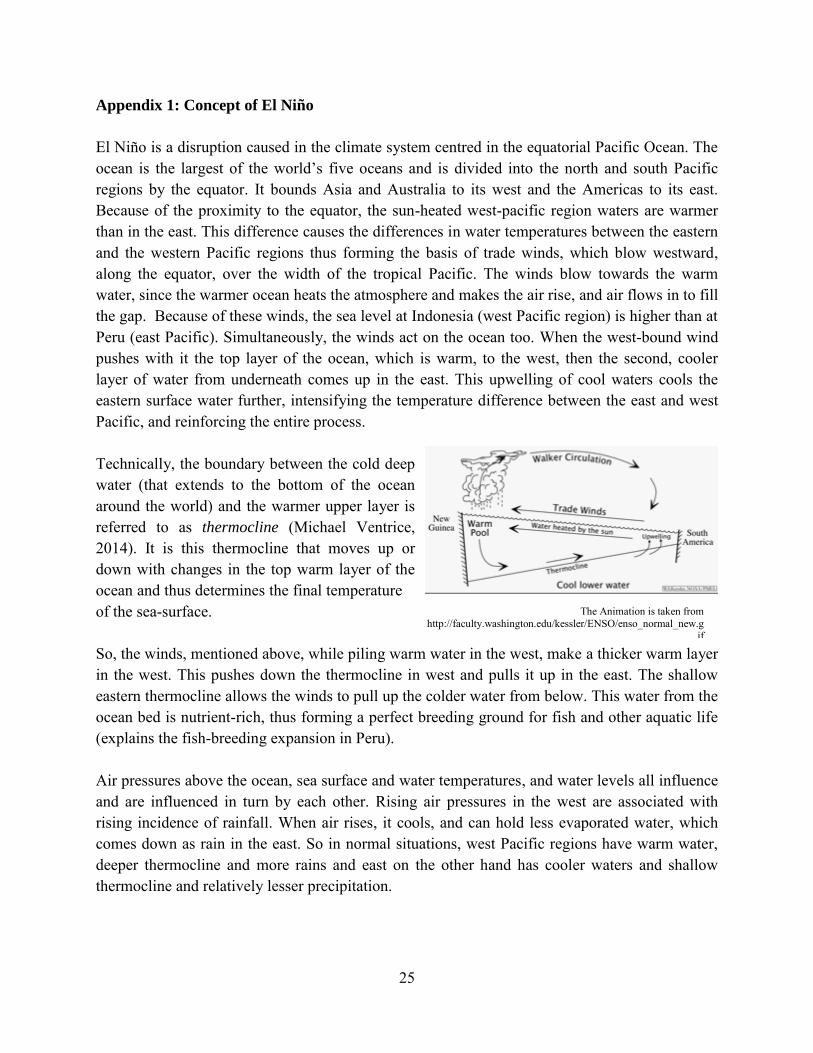
El Niño is a disruption caused in the climate system centred in the equatorial Pacific Ocean. The ocean is the largest of the world’s five oceans and is divided into the north and south Pacific regions by the equator. It bounds Asia and Australia to its west and the Americas to its east. Because of the proximity to the equator, the sun-heated west-pacific region waters are warmer than in the east. This difference causes the differences in water temperatures between the eastern and the western Pacific regions thus forming the basis of trade winds, which blow westward, along the equator, over the width of the tropical Pacific. The winds blow towards the warm water, since the warmer ocean heats the atmosphere and makes the air rise, and air flows in to fill the gap. Because of these winds, the sea level at Indonesia (west Pacific region) is higher than at Peru (east Pacific). Simultaneously, the winds act on the ocean too. When the west-bound wind pushes with it the top layer of the ocean, which is warm, to the west, then the second, cooler layer of water from underneath comes up in the east. This upwelling of cool waters cools the eastern surface water further, intensifying the temperature difference between the east and west Pacific, and reinforcing the entire process. Technically, the boundary between the cold deep water (that extends to the bottom of the ocean around the world) and the warmer upper layer is referred to as thermocline (Michael Ventrice, 2014). It is this thermocline that moves up or down with changes in the top warm layer of the ocean and thus determines the final temperature of the sea-surface. So, the winds, mentioned above, while piling warm water in the west, make a thicker warm layer in the west. This pushes down the thermocline in west and pulls it up in the east. The shallow eastern thermocline allows the winds to pull up the colder water from below. This water from the ocean bed is nutrient-rich, thus forming a perfect breeding ground for fish and other aquatic life (explains the fish-breeding expansion in Peru). Air pressures above the ocean, sea surface and water temperatures, and water levels all influence and are influenced in turn by each other. Rising air pressures in the west are associated with rising incidence of rainfall. When air rises, it cools, and can hold less evaporated water, which comes down as rain in the east. So in normal situations, west Pacific regions have warm water, deeper thermocline and more rains and east on the other hand has cooler waters and shallow thermocline and relatively lesser precipitation.

The Animation is taken from http://faculty.washington.edu/kessler/ENSO/enso_normal_new.g

if

26

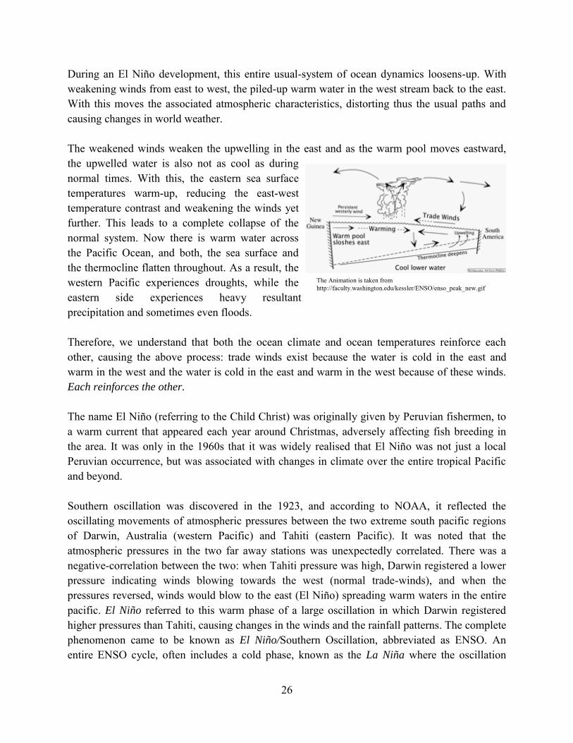
During an El Niño development, this entire usual-system of ocean dynamics loosens-up. With weakening winds from east to west, the piled-up warm water in the west stream back to the east. With this moves the associated atmospheric characteristics, distorting thus the usual paths and causing changes in world weather. The weakened winds weaken the upwelling in the east and as the warm pool moves eastward, the upwelled water is also not as cool as during normal times. With this, the eastern sea surface temperatures warm-up, reducing the east-west temperature contrast and weakening the winds yet further. This leads to a complete collapse of the normal system. Now there is warm water across the Pacific Ocean, and both, the sea surface and the thermocline flatten throughout. As a result, the western Pacific experiences droughts, while the eastern side experiences heavy resultant precipitation and sometimes even floods. Therefore, we understand that both the ocean climate and ocean temperatures reinforce each other, causing the above process: trade winds exist because the water is cold in the east and warm in the west and the water is cold in the east and warm in the west because of these winds. Each reinforces the other.

The name El Niño (referring to the Child Christ) was originally given by Peruvian fishermen, to a warm current that appeared each year around Christmas, adversely affecting fish breeding in the area. It was only in the 1960s that it was widely realised that El Niño was not just a local Peruvian occurrence, but was associated with changes in climate over the entire tropical Pacific and beyond. Southern oscillation was discovered in the 1923, and according to NOAA, it reflected the oscillating movements of atmospheric pressures between the two extreme south pacific regions of Darwin, Australia (western Pacific) and Tahiti (eastern Pacific). It was noted that the atmospheric pressures in the two far away stations was unexpectedly correlated. There was a negative-correlation between the two: when Tahiti pressure was high, Darwin registered a lower pressure indicating winds blowing towards the west (normal trade-winds), and when the pressures reversed, winds would blow to the east (El Niño) spreading warm waters in the entire pacific. El Niño referred to this warm phase of a large oscillation in which Darwin registered higher pressures than Tahiti, causing changes in the winds and the rainfall patterns. The complete phenomenon came to be known as El Niño/Southern Oscillation, abbreviated as ENSO. An entire ENSO cycle, often includes a cold phase, known as the La Niña where the oscillation

The Animation is taken from http://faculty.washington.edu/kessler/ENSO/enso_peak_new.gif

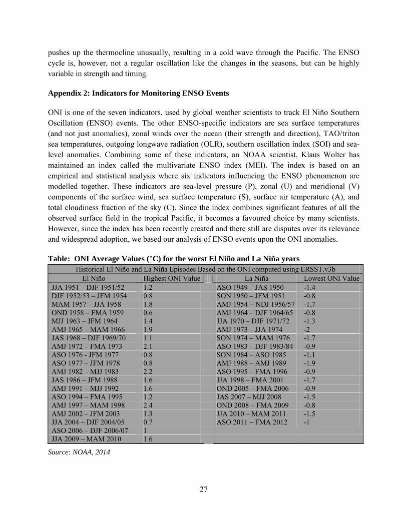
27

pushes up the thermocline unusually, resulting in a cold wave through the Pacific. The ENSO cycle is, however, not a regular oscillation like the changes in the seasons, but can be highly variable in strength and timing. Appendix 2: Indicators for Monitoring ENSO Events

ONI is one of the seven indicators, used by global weather scientists to track El Niño Southern Oscillation (ENSO) events. The other ENSO-specific indicators are sea surface temperatures (and not just anomalies), zonal winds over the ocean (their strength and direction), TAO/triton sea temperatures, outgoing longwave radiation (OLR), southern oscillation index (SOI) and sea-level anomalies. Combining some of these indicators, an NOAA scientist, Klaus Wolter has maintained an index called the multivariate ENSO index (MEI). The index is based on an empirical and statistical analysis where six indicators influencing the ENSO phenomenon are modelled together. These indicators are sea-level pressure (P), zonal (U) and meridional (V) components of the surface wind, sea surface temperature (S), surface air temperature (A), and total cloudiness fraction of the sky (C). Since the index combines significant features of all the observed surface field in the tropical Pacific, it becomes a favoured choice by many scientists. However, since the index has been recently created and there still are disputes over its relevance and widespread adoption, we based our analysis of ENSO events upon the ONI anomalies. Table: ONI Average Values (°C) for the worst El Niño and La Niña years

Historical El Niño and La Niña Episodes Based on the ONI computed using ERSST.v3b El Niño Highest ONI Value La Niña Lowest ONI Value

JJA 1951 – DJF 1951/52 1.2

ASO 1949 – JAS 1950 -1.4 DJF 1952/53 – JFM 1954 0.8

SON 1950 – JFM 1951 -0.8

MAM 1957 – JJA 1958 1.8

AMJ 1954 − NDJ 1956/57 -1.7 OND 1958 – FMA 1959 0.6

AMJ 1964 – DJF 1964/65 -0.8

MJJ 1963 – JFM 1964 1.4

JJA 1970 – DJF 1971/72 -1.3 AMJ 1965 – MAM 1966 1.9

AMJ 1973 – JJA 1974 -2

JAS 1968 – DJF 1969/70 1.1

SON 1974 – MAM 1976 -1.7 AMJ 1972 – FMA 1973 2.1

ASO 1983 – DJF 1983/84 -0.9

ASO 1976 - JFM 1977 0.8

SON 1984 – ASO 1985 -1.1 ASO 1977 – JFM 1978 0.8

AMJ 1988 – AMJ 1989 -1.9

AMJ 1982 – MJJ 1983 2.2

ASO 1995 – FMA 1996 -0.9 JAS 1986 – JFM 1988 1.6

JJA 1998 – FMA 2001 -1.7

AMJ 1991 – MJJ 1992 1.6

OND 2005 – FMA 2006 -0.9 ASO 1994 – FMA 1995 1.2

JAS 2007 – MJJ 2008 -1.5

AMJ 1997 – MAM 1998 2.4

OND 2008 – FMA 2009 -0.8 AMJ 2002 – JFM 2003 1.3

JJA 2010 – MAM 2011 -1.5

JJA 2004 – DJF 2004/05 0.7

ASO 2011 – FMA 2012 -1 ASO 2006 – DJF 2006/07 1

JJA 2009 – MAM 2010 1.6

Source: NOAA, 2014

28

Appendix 3: About IOD and MJO

As per IMD, “the Indian Ocean Dipole (IOD) is a coupled ocean-atmosphere phenomenon in the Indian Ocean. It is normally characterised by the anomalous cooling of SST in the south eastern equatorial Indian Ocean and anomalous warming of SST in the western equatorial Indian Ocean. Associated with these changes, the normal convection situated over the eastern Indian Ocean warm pool shifts to the west and brings heavy rainfall over east Africa and severe droughts/forest fires over the Indonesian region.” A negative IOD is in general is associated with weaker than

normal ISMR. Similarly, a Madden Julian Oscillation (MJO) is another important atmosphere-ocean coupled phenomenon in the tropics influencing the Indian summer monsoon. MJO is a massive weather event consisting of deep convection coupled with atmospheric circulation, moving slowly eastward over the Indian and Pacific Oceans. The MJO involves variations in wind, sea surface temperature (SST), cloudiness, and rainfall. Appendix 4: IMD Calculations

IMD uses a two-stage forecast system for all-India monsoon (June-Sep) rains. The first stage forecast is released in mid-April and the second stage forecast, which is an update of the April forecast, is issued by the end of June, which predicts the rains in the remaining months of monsoons, mainly July. In 2007, IMD adopted an ensemble technique based statistical forecasting system, to forecast the country’s seasonal rainfall. Eight predictors/indicators, which were evaluated to influence the Indian rains, were considered under the system. (See Table below) S. No Predictor (Period) Used for forecasts in 1 North Atlantic Sea Surface Temperature (December + January) April and June 2 Equatorial SE Indian Ocean Sea Surface Temperature

(February + March) April and June

3 East Asia Mean Sea Level Pressure (February + March)

April and June

4 NW Europe Land Surface Air Temperatures (January) April 5 Equatorial Pacific Warm Water Volume (February+March) April 6 Central Pacific (Niño 3.4) Sea Surface Temperature Tendency

(MAM-DJF) June

7 North Atlantic Mean Sea Level Pressure (May) June 8 North Central Pacific Wind at 1.5 Km above sea level (May) June

Source: IMD

29

The top five indicators are used for doing the long range forecast to be released in April. However, the June forecast, which also indicates the forecasts for the months and the season, uses all the eight indicators. Instead of relying on a single model based on these predictors, the forecasting methodology involves creating varied possible models based on different combinations of predictors. According to the IMD, “for April (June) forecast, with 5 predictors, 31 different models were

developed. Out of all the possible models, best few models were selected based on their skill in

predicting monsoon rainfall during a common period.” There are four national climate research centres in the country today that provide experimental LRF: Indian Institute of Tropical Meteorology (IITM), Pune; Space Applications Centre (SAC), Ahmedabad; Centre for Mathematical Modelling and Computer Simulation (CMMACS), Bangalore; and Centre for Development of Advanced Computing (C-DAC), Pune. Internationally, such a LRF is provided by ten International Climate Research Centres, namely: World Meteorological Organization (WMO)’s Lead Centre for Long Range Forecasting - Multi-Model Ensemble (LRFMME), Korea; National Centers for Environmental Prediction (NCEP), USA; Japan Meteorological Agency (JMA), Tokyo; Japan Agency for Marine-Earth Science and Technology (JAMSTEC); International Research Institute for Climate and Society, USA; Meteorological Office, UK; European Centre for Medium Range Weather Forecasts (ECMWF), UK; Meteo France; The Experimental Climate Prediction Center (ECPC), USA, and Asian-Pacific Economic Co-operation (APEC) Climate Centre, Korea.

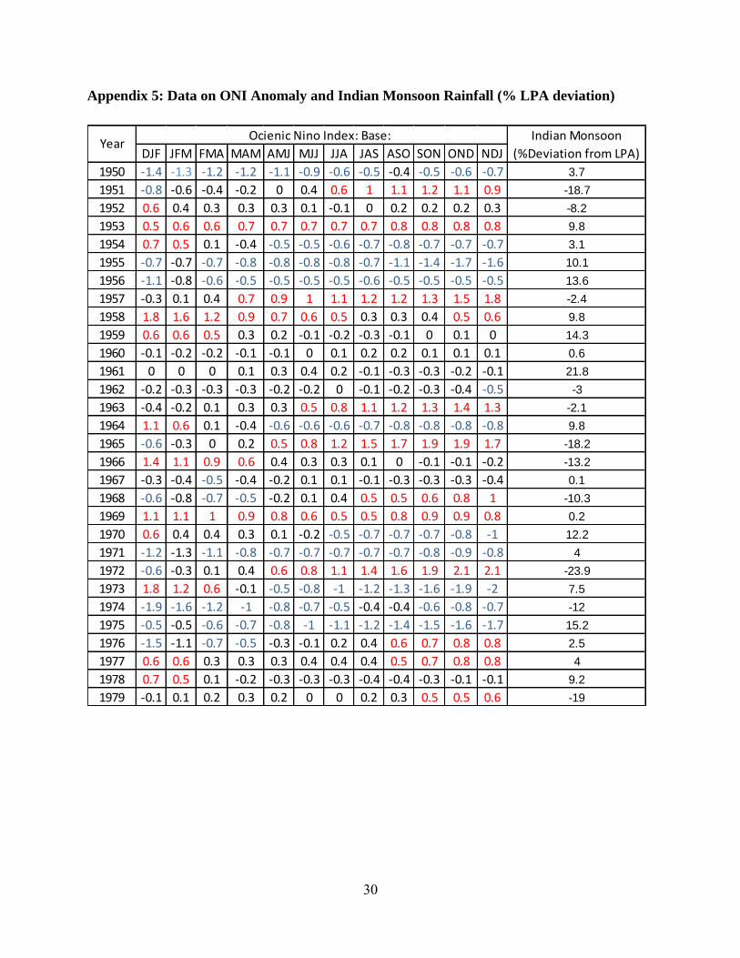
30

Appendix 5: Data on ONI Anomaly and Indian Monsoon Rainfall (% LPA deviation)

DJF JFM FMA MAM AMJ MJJ JJA JAS ASO SON OND NDJ

1950 -1.4 -1.3 -1.2 -1.2 -1.1 -0.9 -0.6 -0.5 -0.4 -0.5 -0.6 -0.7 3.7

1951 -0.8 -0.6 -0.4 -0.2 0 0.4 0.6 1 1.1 1.2 1.1 0.9 -18.7

1952 0.6 0.4 0.3 0.3 0.3 0.1 -0.1 0 0.2 0.2 0.2 0.3 -8.2

1953 0.5 0.6 0.6 0.7 0.7 0.7 0.7 0.7 0.8 0.8 0.8 0.8 9.8

1954 0.7 0.5 0.1 -0.4 -0.5 -0.5 -0.6 -0.7 -0.8 -0.7 -0.7 -0.7 3.1

1955 -0.7 -0.7 -0.7 -0.8 -0.8 -0.8 -0.8 -0.7 -1.1 -1.4 -1.7 -1.6 10.1

1956 -1.1 -0.8 -0.6 -0.5 -0.5 -0.5 -0.5 -0.6 -0.5 -0.5 -0.5 -0.5 13.6

1957 -0.3 0.1 0.4 0.7 0.9 1 1.1 1.2 1.2 1.3 1.5 1.8 -2.4

1958 1.8 1.6 1.2 0.9 0.7 0.6 0.5 0.3 0.3 0.4 0.5 0.6 9.8

1959 0.6 0.6 0.5 0.3 0.2 -0.1 -0.2 -0.3 -0.1 0 0.1 0 14.3

1960 -0.1 -0.2 -0.2 -0.1 -0.1 0 0.1 0.2 0.2 0.1 0.1 0.1 0.6

1961 0 0 0 0.1 0.3 0.4 0.2 -0.1 -0.3 -0.3 -0.2 -0.1 21.8

1962 -0.2 -0.3 -0.3 -0.3 -0.2 -0.2 0 -0.1 -0.2 -0.3 -0.4 -0.5 -3

1963 -0.4 -0.2 0.1 0.3 0.3 0.5 0.8 1.1 1.2 1.3 1.4 1.3 -2.1

1964 1.1 0.6 0.1 -0.4 -0.6 -0.6 -0.6 -0.7 -0.8 -0.8 -0.8 -0.8 9.8

1965 -0.6 -0.3 0 0.2 0.5 0.8 1.2 1.5 1.7 1.9 1.9 1.7 -18.2

1966 1.4 1.1 0.9 0.6 0.4 0.3 0.3 0.1 0 -0.1 -0.1 -0.2 -13.2

1967 -0.3 -0.4 -0.5 -0.4 -0.2 0.1 0.1 -0.1 -0.3 -0.3 -0.3 -0.4 0.1

1968 -0.6 -0.8 -0.7 -0.5 -0.2 0.1 0.4 0.5 0.5 0.6 0.8 1 -10.3

1969 1.1 1.1 1 0.9 0.8 0.6 0.5 0.5 0.8 0.9 0.9 0.8 0.2

1970 0.6 0.4 0.4 0.3 0.1 -0.2 -0.5 -0.7 -0.7 -0.7 -0.8 -1 12.2

1971 -1.2 -1.3 -1.1 -0.8 -0.7 -0.7 -0.7 -0.7 -0.7 -0.8 -0.9 -0.8 4

1972 -0.6 -0.3 0.1 0.4 0.6 0.8 1.1 1.4 1.6 1.9 2.1 2.1 -23.9

1973 1.8 1.2 0.6 -0.1 -0.5 -0.8 -1 -1.2 -1.3 -1.6 -1.9 -2 7.5

1974 -1.9 -1.6 -1.2 -1 -0.8 -0.7 -0.5 -0.4 -0.4 -0.6 -0.8 -0.7 -12

1975 -0.5 -0.5 -0.6 -0.7 -0.8 -1 -1.1 -1.2 -1.4 -1.5 -1.6 -1.7 15.2

1976 -1.5 -1.1 -0.7 -0.5 -0.3 -0.1 0.2 0.4 0.6 0.7 0.8 0.8 2.5

1977 0.6 0.6 0.3 0.3 0.3 0.4 0.4 0.4 0.5 0.7 0.8 0.8 4

1978 0.7 0.5 0.1 -0.2 -0.3 -0.3 -0.3 -0.4 -0.4 -0.3 -0.1 -0.1 9.2

1979 -0.1 0.1 0.2 0.3 0.2 0 0 0.2 0.3 0.5 0.5 0.6 -19

Ocienic Nino Index: Base: Indian Monsoon

(%Deviation from LPA)Year

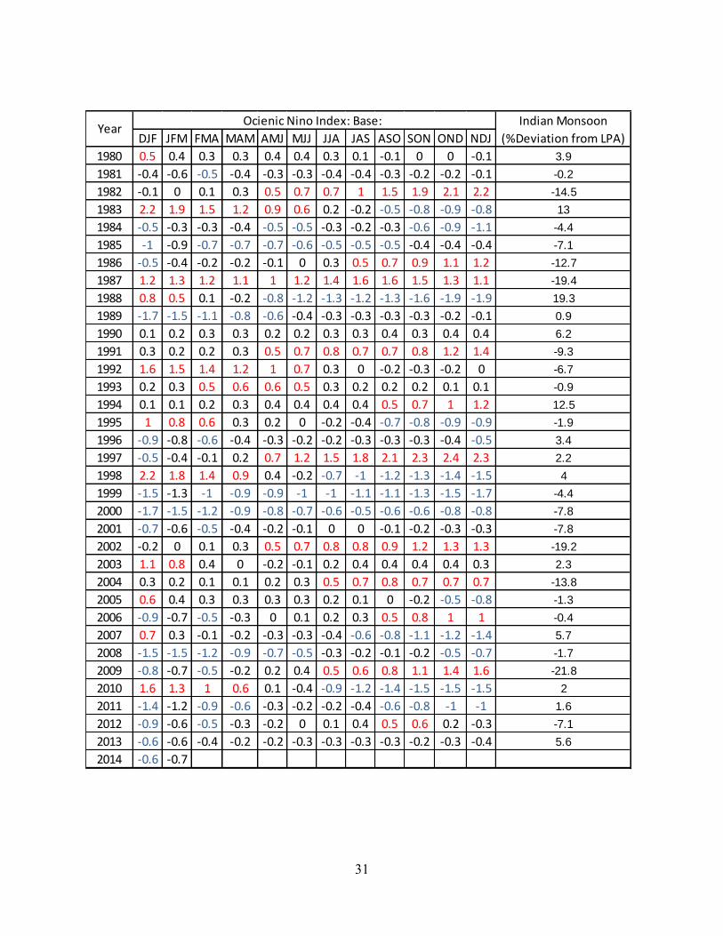
31

DJF JFM FMA MAM AMJ MJJ JJA JAS ASO SON OND NDJ

1980 0.5 0.4 0.3 0.3 0.4 0.4 0.3 0.1 -0.1 0 0 -0.1 3.9

1981 -0.4 -0.6 -0.5 -0.4 -0.3 -0.3 -0.4 -0.4 -0.3 -0.2 -0.2 -0.1 -0.2

1982 -0.1 0 0.1 0.3 0.5 0.7 0.7 1 1.5 1.9 2.1 2.2 -14.5

1983 2.2 1.9 1.5 1.2 0.9 0.6 0.2 -0.2 -0.5 -0.8 -0.9 -0.8 13

1984 -0.5 -0.3 -0.3 -0.4 -0.5 -0.5 -0.3 -0.2 -0.3 -0.6 -0.9 -1.1 -4.4

1985 -1 -0.9 -0.7 -0.7 -0.7 -0.6 -0.5 -0.5 -0.5 -0.4 -0.4 -0.4 -7.1

1986 -0.5 -0.4 -0.2 -0.2 -0.1 0 0.3 0.5 0.7 0.9 1.1 1.2 -12.7

1987 1.2 1.3 1.2 1.1 1 1.2 1.4 1.6 1.6 1.5 1.3 1.1 -19.4

1988 0.8 0.5 0.1 -0.2 -0.8 -1.2 -1.3 -1.2 -1.3 -1.6 -1.9 -1.9 19.3

1989 -1.7 -1.5 -1.1 -0.8 -0.6 -0.4 -0.3 -0.3 -0.3 -0.3 -0.2 -0.1 0.9

1990 0.1 0.2 0.3 0.3 0.2 0.2 0.3 0.3 0.4 0.3 0.4 0.4 6.2

1991 0.3 0.2 0.2 0.3 0.5 0.7 0.8 0.7 0.7 0.8 1.2 1.4 -9.3

1992 1.6 1.5 1.4 1.2 1 0.7 0.3 0 -0.2 -0.3 -0.2 0 -6.7

1993 0.2 0.3 0.5 0.6 0.6 0.5 0.3 0.2 0.2 0.2 0.1 0.1 -0.9

1994 0.1 0.1 0.2 0.3 0.4 0.4 0.4 0.4 0.5 0.7 1 1.2 12.5

1995 1 0.8 0.6 0.3 0.2 0 -0.2 -0.4 -0.7 -0.8 -0.9 -0.9 -1.9

1996 -0.9 -0.8 -0.6 -0.4 -0.3 -0.2 -0.2 -0.3 -0.3 -0.3 -0.4 -0.5 3.4

1997 -0.5 -0.4 -0.1 0.2 0.7 1.2 1.5 1.8 2.1 2.3 2.4 2.3 2.2

1998 2.2 1.8 1.4 0.9 0.4 -0.2 -0.7 -1 -1.2 -1.3 -1.4 -1.5 4

1999 -1.5 -1.3 -1 -0.9 -0.9 -1 -1 -1.1 -1.1 -1.3 -1.5 -1.7 -4.4

2000 -1.7 -1.5 -1.2 -0.9 -0.8 -0.7 -0.6 -0.5 -0.6 -0.6 -0.8 -0.8 -7.8

2001 -0.7 -0.6 -0.5 -0.4 -0.2 -0.1 0 0 -0.1 -0.2 -0.3 -0.3 -7.8

2002 -0.2 0 0.1 0.3 0.5 0.7 0.8 0.8 0.9 1.2 1.3 1.3 -19.2

2003 1.1 0.8 0.4 0 -0.2 -0.1 0.2 0.4 0.4 0.4 0.4 0.3 2.3

2004 0.3 0.2 0.1 0.1 0.2 0.3 0.5 0.7 0.8 0.7 0.7 0.7 -13.8

2005 0.6 0.4 0.3 0.3 0.3 0.3 0.2 0.1 0 -0.2 -0.5 -0.8 -1.3

2006 -0.9 -0.7 -0.5 -0.3 0 0.1 0.2 0.3 0.5 0.8 1 1 -0.4

2007 0.7 0.3 -0.1 -0.2 -0.3 -0.3 -0.4 -0.6 -0.8 -1.1 -1.2 -1.4 5.7

2008 -1.5 -1.5 -1.2 -0.9 -0.7 -0.5 -0.3 -0.2 -0.1 -0.2 -0.5 -0.7 -1.7

2009 -0.8 -0.7 -0.5 -0.2 0.2 0.4 0.5 0.6 0.8 1.1 1.4 1.6 -21.8

2010 1.6 1.3 1 0.6 0.1 -0.4 -0.9 -1.2 -1.4 -1.5 -1.5 -1.5 2

2011 -1.4 -1.2 -0.9 -0.6 -0.3 -0.2 -0.2 -0.4 -0.6 -0.8 -1 -1 1.6

2012 -0.9 -0.6 -0.5 -0.3 -0.2 0 0.1 0.4 0.5 0.6 0.2 -0.3 -7.1

2013 -0.6 -0.6 -0.4 -0.2 -0.2 -0.3 -0.3 -0.3 -0.3 -0.2 -0.3 -0.4 5.6

2014 -0.6 -0.7

Ocienic Nino Index: Base: Indian Monsoon

(%Deviation from LPA)Year

32

Glossary of Terms

Climate: Climate, in a narrow sense, can be defined as the average weather conditions for a particular location and period of time. Droughts: When the monsoon rainfall deficiency exceeds 10 per cent and affects more than 20 per cent of the country’s area, it is categorized as an all-India drought year. Long Period Average (LPA): The LPA is the average or normal rainfall value calculated for all-India or for smaller areas based on an average of actual rainfall received between 1951 and 2000; all-India LPA for monsoon rains is 886.9 mm or 89 cm. El Niño: El Niño, Spanish for "boy child" (because of the tendency of the phenomenon to arrive around Christmas), is an abnormal warming of water in the Equatorial Pacific Ocean every three to five years and can last up to 18 months. La Niña: La Niña means “the little girl”, the opposite of El Niño, and refers to the abnormal

cooling of ocean temperatures in the same Pacific region. Southern Oscillation: The Southern Oscillation is the atmospheric component of El Niño. It is an oscillation in air pressure between the tropical eastern and the western Pacific Ocean waters. ENSO: ENSO is composed of both El Niño and Southern Oscillation. Thus, the oceanic component called El Niño (or La Niña, depending on its phase) and the atmospheric component, the Southern Oscillation. Sea Surface Temperature (SST): SST is defined as the skin temperature of the ocean surface water. Sea Surface Temperature Anomaly (SSTA): Changes in the SST measured from an average temperature during 1971-2000, are called sea-surface temperature anomalies (SSTA) Oceanic Niño Index (ONI): SSTA’s are captured as three months' moving averages in the

Oceanic Niño Index (ONI). When this ONI crosses +0.5 (-0.5) degrees Celsius for five consecutive time periods in a year, the year is declared as El Niño (La Niña) year. Trade Winds: Winds in the tropics generally flow in an east to west direction (easterlies). They are so called because their consistency facilitated transoceanic sailing and commerce. Thermocline: A zone beneath the ocean surface at which the surface water transitions to deep water, and a marked decrease in water temperature occurs.

33

LATEST ICRIER’S WORKING PAPERS NO. TITLE Author YEAR

275 INDIA-PAKISTAN TRADE: AN ANALYSIS OF THE PHARMACEUTICAL SECTOR

MANOJ PANT DEVYANI PANDE

JUNE 2014

274 ENHANCING INDIA-PAKISTAN ECONOMIC COOPERATION: PROSPECTS FOR INDIAN INVESTMENT IN PAKISTAN

PALAKH JAIN AND SAMRIDHI BIMAL

MAY 2014

273 SECURITIES TRANSACTION TAX- CASE STUDY OF INDIA

NEHA MALIK APRIL 2014

272 IMPACT OF TRANSACTION TAXES ON COMMODITY DERIVATIVES TRADING IN INDIA

SAON RAY NEHA MALIK

MARCH 2014

271 FEEDSTOCK FOR THE PETROCHEMICAL INDUSTRY

SAON RAY AMRITA GOLDAR SWATI SALUJA

FEBRUARY 2014

270 USING IPRS TO PROTECT NICHES? EVIDENCE FROM THE INDIAN TEXTILE AND APPAREL INDUSTRY

SUPARNA KARMAKAR MEENU TEWARI

JANUARY 2014

269 MONSOON 2013: ESTIMATING THE IMPACT ON AGRICULTURE

ASHOK GULATI SHWETA SAINI SURBHI JAIN

December 2013

268 REMOTENESS AND UNBALANCED GROWTH: UNDERSTANDING DIVERGENCE ACROSS INDIAN DISTRICTS

SAMARJIT DAS CHETAN GHATE PETER E. ROBERTSON

SEPTEMBER 2013

267 NORMALIZING INDIA PAKISTAN TRADE

NISHA TANEJA MISHITA MEHRA PRITHVIJIT MUKHERJEE SAMRIDHI BIMAL ISHA DAYAL

SEPTEMBER 2013

34

About ICRIER Established in August 1981, ICRIER is an autonomous, policy-oriented, not-for-profit, economic policy think tank. ICRIER's main focus is to enhance the knowledge content of policy making by undertaking analytical research that is targeted at informing India's policy makers and also at improving the interface with the global economy. ICRIER's office is located in the institutional complex of India Habitat Centre, New Delhi. ICRIER's Board of Governors includes leading academicians, policymakers, and representatives from the private sector. Dr. Isher Ahluwalia is ICRIER's chairperson. Dr. Rajat Kathuria is Director and Chief Executive. ICRIER conducts thematic research in the following seven thrust areas:

Macro-economic Management in an Open Economy

Trade, Openness, Restructuring and Competitiveness

Financial Sector Liberalisation and Regulation

WTO-related Issues

Regional Economic Co-operation with Focus on South Asia Strategic Aspects of India's International Economic Relations

Environment and Climate Change

To effectively disseminate research findings, ICRIER organises workshops, seminars and conferences to bring together academicians, policymakers, representatives from industry and media to create a more informed understanding on issues of major policy interest. ICRIER routinely invites distinguished scholars and policymakers from around the world to deliver public lectures and give seminars on economic themes of interest to contemporary India.