World Energy Projection System Plus: Overview · The World Energy Projection System Plus (WEPS+) is the energy modeling system used to produce the IEO2017. The complete WEPS+ system

World Energy Projection System Plus:

Overview

December 2017

Independent Statistics & Analysis

www.eia.gov

U.S. Department of Energy

Washington, DC 20585

U.S. Energy Information Administration | World Energy Projection System Plus: Overview i

This report was prepared by the U.S. Energy Information Administration (EIA), the statistical and

analytical agency within the U.S. Department of Energy. By law, EIA’s data, analyses, and forecasts are

independent of approval by any other officer or employee of the United States Government. The views

in this report therefore should not be construed as representing those of the U.S. Department of Energy

or other federal agencies.

December 2017

U.S. Energy Information Administration | World Energy Projection System Plus: Overview 1

Contents

1. Introduction .............................................................................................................................................. 3

Purpose of this report .............................................................................................................................. 3

System summary ..................................................................................................................................... 3

2. Common Database .................................................................................................................................... 7

3. Global Activity Model ................................................................................................................................ 8

4. Residential Model ..................................................................................................................................... 9

5. Commercial Model .................................................................................................................................. 11

6. Industrial Model ...................................................................................................................................... 13

7. Transportation Model ............................................................................................................................. 17

8. Electricity Model ..................................................................................................................................... 19

9. District Heat Model ................................................................................................................................. 22

10. Petroleum Model .................................................................................................................................. 24

11. Natural Gas Model ................................................................................................................................ 25

12. Coal Model ............................................................................................................................................ 27

13. Refinery Model...................................................................................................................................... 28

14. Greenhouse Gases Model ..................................................................................................................... 30

15. Main Model and Convergence Process ................................................................................................ 31

December 2017


Table of Tables

Table 1: Core models .................................................................................................................................... 4

Table 2. Regional aggregation ....................................................................................................................... 6

Table 3. Residential model input data series ................................................................................................ 9

Table 4. Residential model output data series ........................................................................................... 10

Table 5. Commercial model input data series ............................................................................................ 11

Table 6. Commercial model output data series .......................................................................................... 12

Table 7. Industrial model input data series ................................................................................................ 15

Table 8. Industrial output data series ......................................................................................................... 15

Table 9. Transportation model input data series........................................................................................ 17

Table 10. Transportation model input data series...................................................................................... 18

Table 11. Transportation model output data series ................................................................................... 18

Table 12. Electricity model input data series .............................................................................................. 20

Table 13. Electricity model output data series ........................................................................................... 21

Table 14. District heat model input data series .......................................................................................... 22

Table 15. District heat model output data series ....................................................................................... 23

Table 16. Petroleum model input data series ............................................................................................. 24

Table 17. Petroleum Model output data series .......................................................................................... 24

Table 18. Natural gas model input data series ........................................................................................... 26

Table 19. Natural gas model output data series ......................................................................................... 26

Table 20. Coal model input data series ....................................................................................................... 27

Table 21. Coal model output data series .................................................................................................... 27

Table 22. Refinery model input data series ................................................................................................ 28

Table 23. Refinery model output data series .............................................................................................. 29

Table 24. Summary of the convergence process ........................................................................................ 32

Table of Figures

Figure 1. World Energy Projection System Plus (WEPS+) model sequence .................................................. 5

Figure 2. Stock/flow capacity adjustments over time ................................................................................ 14

Figure 3. Illustration of convergence in WEPS+ .......................................................................................... 31

December 2017


1. Introduction

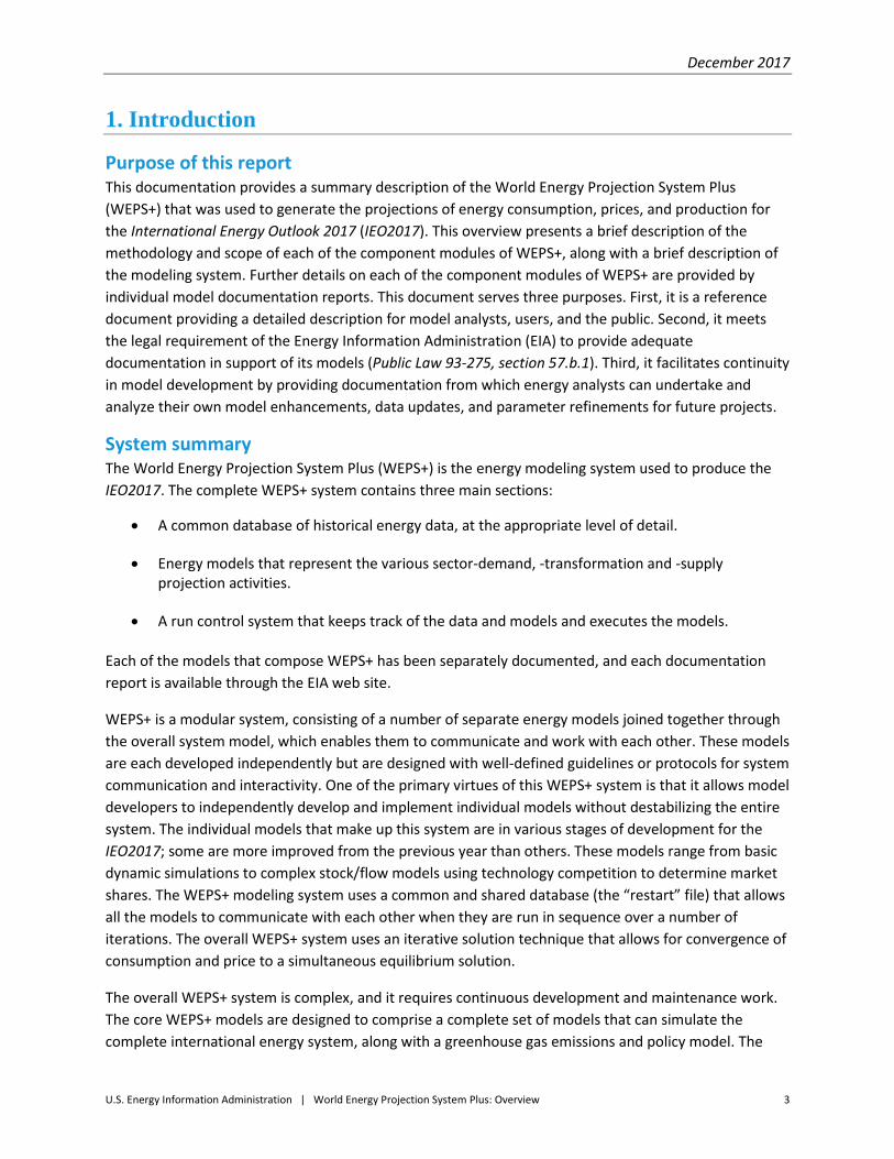
Purpose of this report This documentation provides a summary description of the World Energy Projection System Plus

(WEPS+) that was used to generate the projections of energy consumption, prices, and production for

the International Energy Outlook 2017 (IEO2017). This overview presents a brief description of the

methodology and scope of each of the component modules of WEPS+, along with a brief description of

the modeling system. Further details on each of the component modules of WEPS+ are provided by

individual model documentation reports. This document serves three purposes. First, it is a reference

document providing a detailed description for model analysts, users, and the public. Second, it meets

the legal requirement of the Energy Information Administration (EIA) to provide adequate

documentation in support of its models (Public Law 93-275, section 57.b.1). Third, it facilitates continuity

in model development by providing documentation from which energy analysts can undertake and

analyze their own model enhancements, data updates, and parameter refinements for future projects.

System summary The World Energy Projection System Plus (WEPS+) is the energy modeling system used to produce the

IEO2017. The complete WEPS+ system contains three main sections:

A common database of historical energy data, at the appropriate level of detail.

Energy models that represent the various sector-demand, -transformation and -supply projection activities.

A run control system that keeps track of the data and models and executes the models.

Each of the models that compose WEPS+ has been separately documented, and each documentation

report is available through the EIA web site.

WEPS+ is a modular system, consisting of a number of separate energy models joined together through

the overall system model, which enables them to communicate and work with each other. These models

are each developed independently but are designed with well-defined guidelines or protocols for system

communication and interactivity. One of the primary virtues of this WEPS+ system is that it allows model

developers to independently develop and implement individual models without destabilizing the entire

system. The individual models that make up this system are in various stages of development for the

IEO2017; some are more improved from the previous year than others. These models range from basic

dynamic simulations to complex stock/flow models using technology competition to determine market

shares. The WEPS+ modeling system uses a common and shared database (the “restart” file) that allows

all the models to communicate with each other when they are run in sequence over a number of

iterations. The overall WEPS+ system uses an iterative solution technique that allows for convergence of

consumption and price to a simultaneous equilibrium solution.

The overall WEPS+ system is complex, and it requires continuous development and maintenance work.

The core WEPS+ models are designed to comprise a complete set of models that can simulate the

complete international energy system, along with a greenhouse gas emissions and policy model. The

December 2017


system also includes models that perform preprocessing and post-processing, including various final

reporting programs. The current core set of models is outlined in Table 1.

Table 1: Core models

Type of Activity WEPS+ Model

1. Global Activity Model

Demand Models

2. Residential Model

3. Commercial Model

4. Industrial Model

5. Transportation Model

Transformation Models

6. Electricity Model

7. District Heat Model

Supply Models

8. Petroleum Model

9. Natural Gas Model

10. Coal Model

11. Refinery (Part 1 & 2)

12. Greenhouse Gas Model

13. Main Model

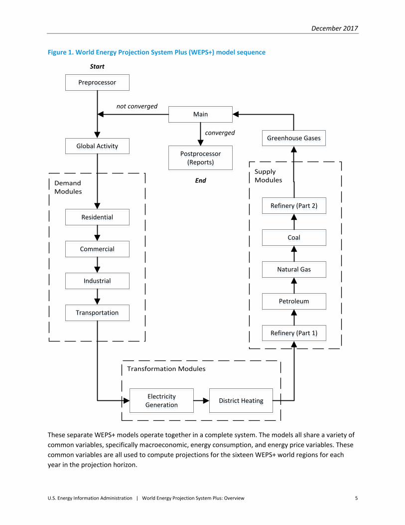
The flowchart in Figure 1 illustrates the sequence of model operations in WEPS+. Each model is run

independently but reads and writes to a common and shared database (the “restart” file) in order to

communicate with other models (not shown in the flowchart). Each model completes its execution

before the next model in the sequence is started up. The system begins with a common database (also

known as the ‘restart file’) from a previous system run so that it starts with “seed” values for prices and

consumption. Each model is run in turn before the system runs the main model, which then determines

if the system has converged (this is described in greater detail in Chapter 15). If the system does not

converge, it begins another sequence (iteration). If it does converge, it then finishes up with report

writing.

December 2017


Figure 1. World Energy Projection System Plus (WEPS+) model sequence

These separate WEPS+ models operate together in a complete system. The models all share a variety of

common variables, specifically macroeconomic, energy consumption, and energy price variables. These

common variables are all used to compute projections for the sixteen WEPS+ world regions for each

year in the projection horizon.

DemandModules

SupplyModules

Transformation Modules

PreprocessorPreprocessor

Global ActivityGlobal ActivityGreenhouse GasesGreenhouse Gases

Refinery (Part 2)Refinery (Part 2)

Electricity Generation

Electricity Generation District HeatingDistrict Heating

ResidentialResidential

CommercialCommercial

IndustrialIndustrial

TransportationTransportation

CoalCoal

Natural GasNatural Gas

PetroleumPetroleum

Refinery (Part 1)Refinery (Part 1)

MainMain

Postprocessor(Reports)

Postprocessor(Reports)

converged

not converged

Start

End

December 2017


The sixteen WEPS+ world regions consist of countries and country groupings within the broad divide of

Organization of Economic Cooperation and Development (OECD) countries and non-OECD countries.

These regions are shown in Table 2.

Table 2. Regional aggregation

OECD Regions Non-OECD Regions

United States Russia

Canada Other Non-OECD Europe and Eurasia

Mexico/Chile China

OECD Europe India

Japan Other Non-OECD Asia

Australia/New Zealand Middle East

South Korea Africa

Brazil

Other Non-OECD Americas

The following report provides an overview of the various WEPS+ modules as used for the IEO2017.

System archival citation This documentation refers to the World Energy Projection System Plus (WEPS+) Overview, as archived

for the International Energy Outlook 2017 (IEO2017).

WEPS+ source code for the most recent IEO is available at

https://www.eia.gov/outlooks/ieo/ieowepsplus_sourcecode.php. Previous year’s WEPS+ code is also

available. For example, the WEPS+ source code for IEO2016 can be downloaded from

https://www.eia.gov/outlooks/archive/ieo16/ieowepsplus_sourcecode.php

System contact Michael Cole

U.S. Energy Information Administration

U.S. Department of Energy

1000 Independence Avenue, SW

Washington, D.C. 20585

Telephone: (202) 586-7209

E-mail: [email protected]

Organization of this report Chapter 2 of this report provides detail on the data sources used by WEPS+ as well as an explanation of

how data is shared by the component models within the system. Chapters 3 – 15 each provide an

overview of one of the component models within WEPS+, including the data inputs and outputs for each

model. Chapter 15 also explains and illustrates the model convergence process.

https://www.eia.gov/outlooks/ieo/ieowepsplus_sourcecode.php

https://www.eia.gov/outlooks/archive/ieo16/ieowepsplus_sourcecode.php

mailto:[email protected]

December 2017


2. Common Database

There are several key historical data sources used for WEPS+:

The U.S. Energy Information Administration’s (EIA) International Energy Statistics (IES) database (https://www.eia.gov/beta/international/) provides non-U.S. country-level consumption data for liquids, natural gas, coal, nuclear energy, and hydroelectric and other renewables consumed for electricity generation. IES also includes thermal, nuclear, hydroelectric, and other renewables (wind, biomass and waste, geothermal, and solar/tide/wave/fuel cell) electricity generation and installed generating capacity.

The international data produced and maintained by the International Energy Agency in Paris (referred to as IEA/Paris) as part of its energy balances database provides country-level consumption data for a wide variety of “flows” (sectors and users) and for a wide variety of “products” (detailed petroleum products, coal types, renewable sources, etc.). EIA uses these detailed data to derive the historical, end-use sector data used in WEPS+ demand models.

Historical data and projections for the United States are extracted from the most recent EIA

Annual Energy Outlook (AEO2017 for IEO2017).

The EIA data source provides the overall consumption levels, while the IEA/Paris data provides

consumption information at more detailed levels. The IEA/Paris data therefore must be calibrated (or

“shared”) to agree with the EIA data.

Because of the detail and subtlety of the underlying IEA/Paris data, and because of the need for

calibrating it to the EIA data, a considerable amount of effort goes into the organization and processing

of this initial data. This high level of effort is also necessary to accomplish the following objectives:

Provide industry-level detail for the Industrial Model

Provide mode-level detail for the Transportation Model

Coordinate with capacity and generation data at various levels for the Electricity Model

Find and correct any errors, data gaps, or inconsistencies

The process is largely automated, but it has been necessary to carefully review and modify it each year.

The resulting detailed data are made available to each of the models for their initialization. To do this,

the historical data are put into the common, shared database known as the “restart” file.

The primary purpose of the common database, however, is to function as a repository for the wide

range of variables that are communicated and shared among all the models making up the system. Any

individual model may use much more detailed data from its own input files if necessary, but it will

communicate with other models using the common level of detail in the common database. Each model,

when it is executed, first reads the common database to obtain the shared data that it needs as it runs.

When the model is finished with its calculations, it writes results to the common database for use by the

other models. Basic descriptions of the data that are communicated for each of the models in the

system are provided in the following chapters of this report.

https://www.eia.gov/beta/international/

December 2017


3. Global Activity Model

The commercially-available Oxford Economics Global Economic Model (GEM) and Global Industry Model

(GIM) are used to generate projections of gross domestic product (GDP) and gross output for the various

IEO countries and regions and their respective industrial sectors, given energy inputs from WEPS+. The

theoretical structure of GEM differentiates between the short-term and long-term projections for each

country, with extensive coverage of the links among different economies. GEM produces GDP outputs

for use with WEPS+ and also provides drivers for GIM. The structure of GIM, which calculates gross

output in the IEO sectors for each country or region in WEPS+, is based on input-output relationships. It

calculates gross output in the IEO sectors for each country or region in WEPS+

December 2017


4. Residential Model

The WEPS+ Residential Model projects household energy consumption, excluding on-road

transportation, which is projected in the Transportation Model. The model focuses on nine energy

sources in each of the sixteen WEPS+ regions over the projection horizon. The Residential Model

primarily uses a dynamic econometric equation for the key energy sources, basing the projection on

household income assumptions, residential retail energy prices for seven fuels, and an assumed future

trend. The dynamic equation uses a lagged dependent variable to imperfectly represent fuel stock

accumulation in the calculation of retail fuel prices for each region over time. The income and price

projections are available to the Residential Model from the WEPS+ Global Activity Model and supply

models through the common database. The trend factor is meant to represent continuing impacts on

energy use not directly represented in household income and prices, and may include the effects of a

variety of behavioral, structural, and policy-induced activities.

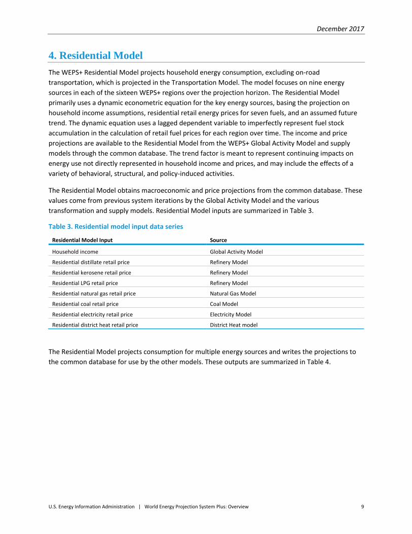
The Residential Model obtains macroeconomic and price projections from the common database. These

values come from previous system iterations by the Global Activity Model and the various

transformation and supply models. Residential Model inputs are summarized in Table 3.

Table 3. Residential model input data series

Residential Model Input Source

Household income Global Activity Model

Residential distillate retail price Refinery Model

Residential kerosene retail price Refinery Model

Residential LPG retail price Refinery Model

Residential natural gas retail price Natural Gas Model

Residential coal retail price Coal Model

Residential electricity retail price Electricity Model

Residential district heat retail price District Heat model

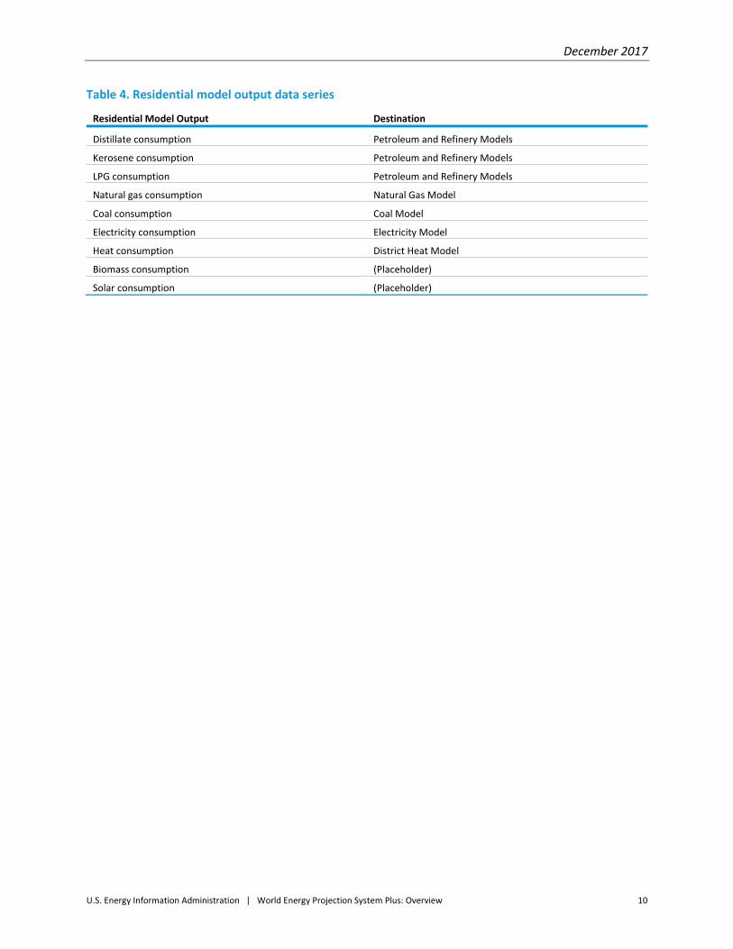
The Residential Model projects consumption for multiple energy sources and writes the projections to

the common database for use by the other models. These outputs are summarized in Table 4.

December 2017


Table 4. Residential model output data series

Residential Model Output Destination

Distillate consumption Petroleum and Refinery Models

Kerosene consumption Petroleum and Refinery Models

LPG consumption Petroleum and Refinery Models

Natural gas consumption Natural Gas Model

Coal consumption Coal Model

Electricity consumption Electricity Model

Heat consumption District Heat Model

Biomass consumption (Placeholder)

Solar consumption (Placeholder)

December 2017


5. Commercial Model

The WEPS+ Commercial Model projects energy use that takes place in commercial buildings and

activities. It also includes municipal activity, such as street lighting. The model projects commercial

consumption for eleven energy sources in each of the sixteen WEPS+ regions. The Commercial Model

primarily uses a dynamic econometric equation for consumption of key energy sources, basing the

projection on assumptions for gross output of the services sector, commercial retail energy prices for

nine fuels, and an assumed future trend. The dynamic equation uses a lagged dependent variable to

imperfectly represent stock accumulation in the calculation of retail fuel prices for each region over

time. The service sector gross output and price projections are available to the Commercial Model from

the WEPS+ Global Activity Model and the supply models through the common database. The trend

factor is meant to represent continuing impacts on energy use not directly represented in the GDP and

price and may include the effects of a variety of behavioral, structural, and policy-induced activities.

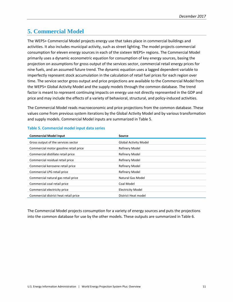
The Commercial Model reads macroeconomic and price projections from the common database. These

values come from previous system iterations by the Global Activity Model and by various transformation

and supply models. Commercial Model inputs are summarized in Table 5.

Table 5. Commercial model input data series

Commercial Model Input Source

Gross output of the services sector Global Activity Model

Commercial motor gasoline retail price Refinery Model

Commercial distillate retail price Refinery Model

Commercial residual retail price Refinery Model

Commercial kerosene retail price Refinery Model

Commercial LPG retail price Refinery Model

Commercial natural gas retail price Natural Gas Model

Commercial coal retail price Coal Model

Commercial electricity price Electricity Model

Commercial district heat retail price District Heat model

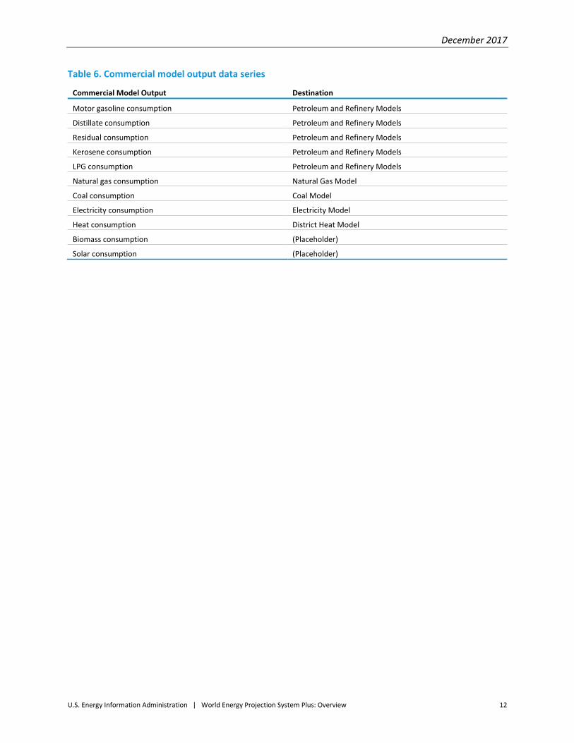
The Commercial Model projects consumption for a variety of energy sources and puts the projections

into the common database for use by the other models. These outputs are summarized in Table 6.

December 2017


Table 6. Commercial model output data series

Commercial Model Output Destination

Motor gasoline consumption Petroleum and Refinery Models


Residual consumption Petroleum and Refinery Models







Biomass consumption (Placeholder)

Solar consumption (Placeholder)

December 2017


6. Industrial Model

The WEPS+ Industrial Model projects the amount of energy that is directly consumed as a fuel or as a

feedstock by industrial processes and activities. It includes both manufacturing industries and non-

manufacturing industries such as construction, agriculture and mining. It projects industrial

consumption for eighteen energy sources in each of the sixteen WEPS+ regions over the projection

horizon. The Industrial Model is a structured, industry-level, stock/flow model that uses gross output

from the Global Activity Model as its primary driver. The model also uses retail energy prices for twelve

energy sources. These drivers are available to the Industrial Model from the WEPS+ global activity and

supply models through the shared common database.

The Industrial Model projects energy consumption in multiple separate industries identified according to

their energy consumption characteristics. The industries modeled include Paper, Basic Chemicals,

Refineries, Iron and Steel, Motor Vehicles, and others. For a complete list, see the separate Industrial

Model documentation.

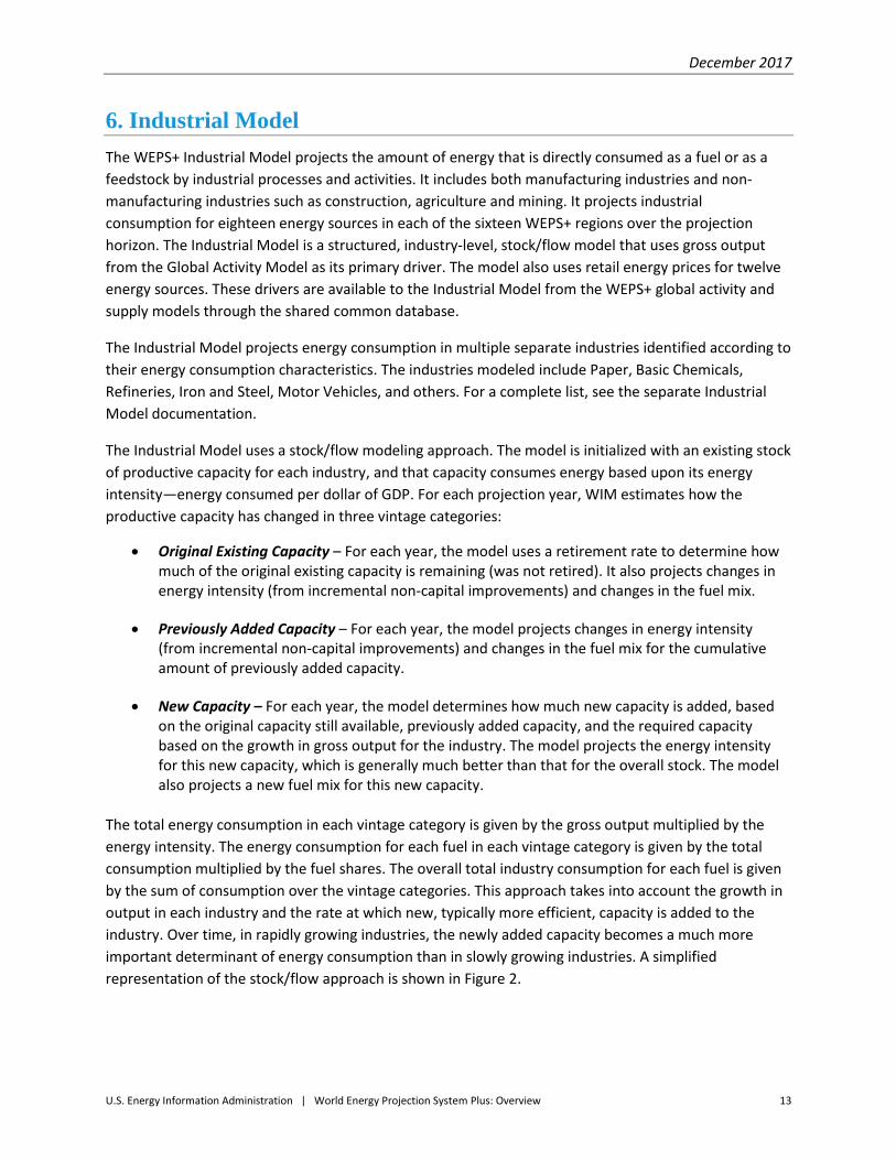
The Industrial Model uses a stock/flow modeling approach. The model is initialized with an existing stock

of productive capacity for each industry, and that capacity consumes energy based upon its energy

intensity—energy consumed per dollar of GDP. For each projection year, WIM estimates how the

productive capacity has changed in three vintage categories:

Original Existing Capacity – For each year, the model uses a retirement rate to determine how much of the original existing capacity is remaining (was not retired). It also projects changes in energy intensity (from incremental non-capital improvements) and changes in the fuel mix.

Previously Added Capacity – For each year, the model projects changes in energy intensity (from incremental non-capital improvements) and changes in the fuel mix for the cumulative amount of previously added capacity.

New Capacity – For each year, the model determines how much new capacity is added, based on the original capacity still available, previously added capacity, and the required capacity based on the growth in gross output for the industry. The model projects the energy intensity for this new capacity, which is generally much better than that for the overall stock. The model also projects a new fuel mix for this new capacity.

The total energy consumption in each vintage category is given by the gross output multiplied by the

energy intensity. The energy consumption for each fuel in each vintage category is given by the total

consumption multiplied by the fuel shares. The overall total industry consumption for each fuel is given

by the sum of consumption over the vintage categories. This approach takes into account the growth in

output in each industry and the rate at which new, typically more efficient, capacity is added to the

industry. Over time, in rapidly growing industries, the newly added capacity becomes a much more

important determinant of energy consumption than in slowly growing industries. A simplified

representation of the stock/flow approach is shown in Figure 2.

December 2017


Figure 2. Stock/flow capacity adjustments over time

The Industrial Model reads macroeconomic and price projections from the common database. These

values come from previous system iterations by the Global Activity Model and by various transformation

and supply models. Industrial Model inputs are summarized in Table 7.

Time

Capacity

Total capacity

Remaining

original

capacity

Remaining original capacity

Added

capacity

Added capacity

December 2017


Table 7. Industrial model input data series

Industrial Model Input Source

Gross domestic product Global Activity Model

Industrial motor gasoline retail price Refinery Model

Industrial distillate retail price Refinery Model

Industrial residual fuel oil retail price Refinery Model

Industrial kerosene retail price Refinery Model

Industrial LPG retail price Refinery Model

Industrial other petroleum retail price Refinery Model

Industrial natural gas retail price Natural Gas Model

Industrial coal retail price Coal Model

Industrial electricity retail price Electricity Model

Industrial district heat retail price District Heat Model

The Industrial Model projects consumption for multiple energy sources and writes the projections to the

common database for use by the other models. These outputs are summarized in Table 8.

Table 8. Industrial output data series

Industrial Model Output Source






Petroleum coke consumption Petroleum and Refinery Models

Sequestered petroleum consumption Petroleum and Refinery Models

Other petroleum consumption Petroleum and Refinery Models

Crude oil consumption (direct use) Petroleum and Refinery Models





Waste consumption Reporting

Biomass consumption Reporting

Geothermal consumption Reporting

Solar consumption Reporting

Other renewable consumption Reporting

December 2017


The Industrial Model requires a significant amount of initial data, along with many coefficients. The data

for the initial consumption is available from the IEA/Paris database (calibrated to the EIA data) described

earlier. The coefficients are based on an analysis that compared existing industrial energy intensities

among various regions particularly with a view towards the efficiency “gap” that is found between

developed and developing regions. Based upon this comparison, analyst judgment was used to

determine the relative new energy intensities. Analyst judgment was also used to develop several other

coefficients such as drivers for retirement rates, rates of change of remaining and added energy

intensities, and sensitivities to fuel prices.

December 2017


7. Transportation Model

The WEPS+ Transportation Model (ITEDD) projects the amount of energy that is consumed to provide

passenger and freight transportation services. This includes personal household on-road transportation

in light duty vehicles (counted here rather than in the residential sector model). This also includes fuel

consumed by natural gas pipelines, and small amounts of lubricants and waxes. The model projects

transportation consumption for fourteen energy sources in each of the sixteen WEPS regions over the

projection horizon. The Transportation Model provides an accounting framework that considers energy

service demand and service intensity (efficiency) for the overall stock of vehicles. The service demand is

a measure of overall passenger miles for passenger services and overall ton miles for freight services.

The service intensity is a measure of passenger miles per unit of energy expended (in Btu) for passenger

services and ton miles per unit of energy expended (in Btu) for freight services.

The Transportation Model categorizes transportation services for passengers and freight in four modes

consisting of road, rail, water and air. These modes are also broken down into sub-modes as shown in

Table 9.

Table 9. Transportation model input data series

Transportation Mode Transportation Sub-Mode

1. Road

1a. Light Duty Vehicles

1b. Two/Three Wheel Vehicles

1c. Buses

1d. Freight Trucks

1e. Other Trucks

2. Rail 2a. Passenger

2b. Freight

3. Water 3a. Domestic

3b. International

4. Air 4a. All Air

The Transportation Model performs the following functions:

Uses a bottom-up approach to estimate demand for transportation energy by mode

(road, rail, air, and marine) and vehicle type (light-duty vehicles, freight trucks,

passenger rail, etc.);

Estimates transportation energy consumption by fuel and region;

Estimates vehicle stocks by vehicle type and region.

The Transportation Model reads macroeconomic and price projections from the common database.

These values come from previous system iterations by the Global Activity Model and various

transformation and supply models. Transportation Model inputs are summarized in Table 10.

December 2017


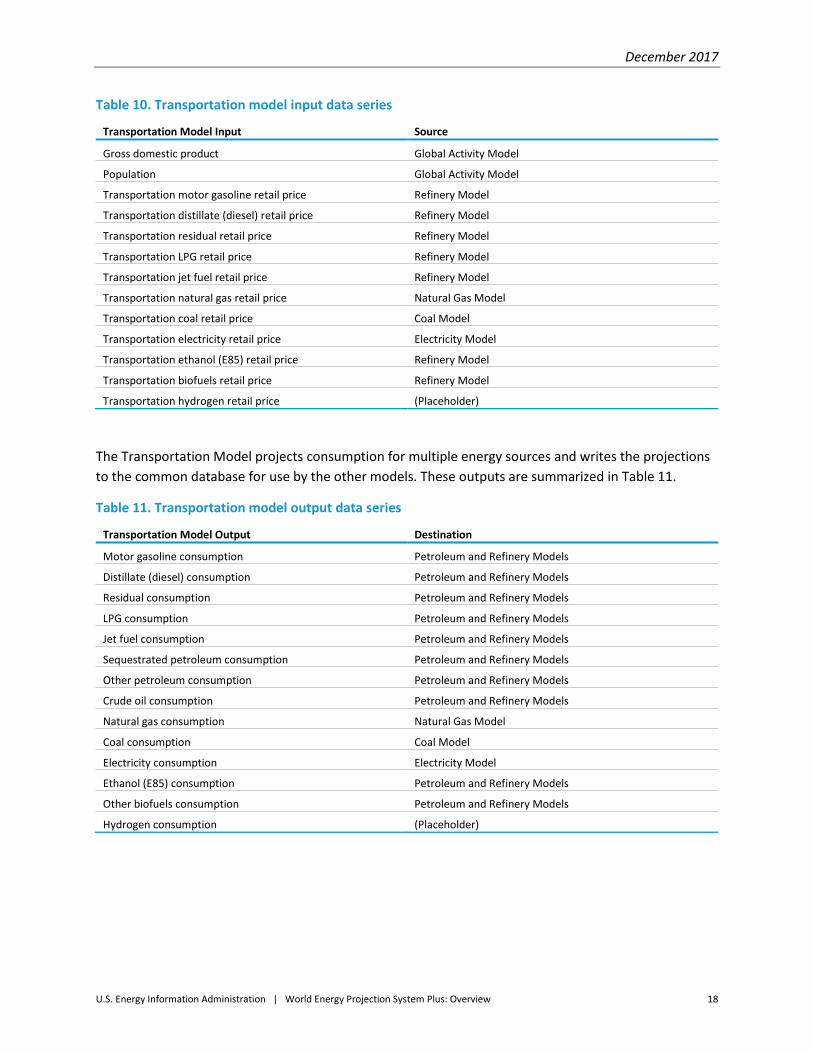
Table 10. Transportation model input data series

Transportation Model Input Source

Gross domestic product Global Activity Model

Population Global Activity Model

Transportation motor gasoline retail price Refinery Model

Transportation distillate (diesel) retail price Refinery Model

Transportation residual retail price Refinery Model

Transportation LPG retail price Refinery Model

Transportation jet fuel retail price Refinery Model

Transportation natural gas retail price Natural Gas Model

Transportation coal retail price Coal Model

Transportation electricity retail price Electricity Model

Transportation ethanol (E85) retail price Refinery Model

Transportation biofuels retail price Refinery Model

Transportation hydrogen retail price (Placeholder)

The Transportation Model projects consumption for multiple energy sources and writes the projections

to the common database for use by the other models. These outputs are summarized in Table 11.

Table 11. Transportation model output data series

Transportation Model Output Destination


Distillate (diesel) consumption Petroleum and Refinery Models



Jet fuel consumption Petroleum and Refinery Models

Sequestrated petroleum consumption Petroleum and Refinery Models

Other petroleum consumption Petroleum and Refinery Models

Crude oil consumption Petroleum and Refinery Models




Ethanol (E85) consumption Petroleum and Refinery Models

Other biofuels consumption Petroleum and Refinery Models

Hydrogen consumption (Placeholder)

December 2017


8. Electricity Model

The WEPS+ Electricity Model projects the generation of electricity to satisfy the electricity demands

projected by the end-use demand models. The model forecasts fuel consumed, electricity generated,

and generation capacity by each technology for thirteen energy sources in each of the sixteen

international regions over the projection horizon. The Electricity Model also projects end-use electricity

prices for each of four demand sectors in each of the sixteen international regions.

The Electricity Model is a technology-based, least-cost model that uses a logit function to estimate

levelized cost for new generation technology in three load segments. It then uses the levelized costs to

project market shares for each technology. The model accounts for a slate of available new technologies

along with their corresponding characteristics. These technology characteristics vary by region and

include heat rates (efficiency), capital cost (per kilowatt-hour), fixed operating cost, variable operating

cost, availability factor, and more. For each fuel type, the model features different technology

representations, including carbon capture and storage (CCS) technologies.

The Electricity Model initially estimates the total amount of generation that is required in each region by

adding up the electricity demand from each sector and accounting for losses from transmission and

distribution. These generation requirements are allocated to seasons and load segments based upon an

overall system load curve. Each load curve describes how much of the annual load is consumed within

specified periods of time in three seasons (summer, winter, and spring/fall). The periods of time are

specified as percentages of the year and the amounts of the load are specified as percentages of the

load. The model builds the system load curve based upon the load curves for each sector and each

region and the relative weight of demand in each sector and region. The model then retires the existing

capacity as necessary and determines how much total capacity is available for generation in each load

segment and season.

Both nuclear capacity and renewable capacity are determined outside of the least-cost logit competition

for fossil fuels. The total amount of nuclear capacity is generally policy driven and is exogenous to the

model. However, to a large extent, renewable policies are input to the model and the model determines

the amount of renewable capacity based upon policies that relate it to fossil capacity or to other goals.

For each renewable and nuclear technology, the model determines the amount of new capacity added

in a given year by looking at the difference between the total capacity for that year and the capacity

available (and surviving) from the previous year.

The Electricity Model then uses a load dispatch algorithm to determine how the surviving capacity, along

with the new nuclear and renewable capacity, is used to generate electricity. That consequently

determines the amount of generation currently available. The generation available is compared to the

generation requirements to determine how much new fossil generation is required. The new fossil

generation is determined in a capacity planning algorithm that calculates levelized cost for each new

technology that is available in the slate. The technology costs are then competed against each other in a

logit-based, market share algorithm that gives more market share to lower cost technologies – the

amount of market share is based upon a logit coefficient. The load dispatch and capacity planning

algorithms are run within different load segments with different tradeoffs between fixed and variable

December 2017


costs resulting in different technology choices and capacity factors. The model also takes into account a

reserve margin and has a learning algorithm for costs and heat rates.

The capacity choices that are made in capacity planning, the determination of how capacity is used for

generation in the load dispatch, and the heat rates (efficiencies) determine the amount of fuel

consumed by each technology. The Electricity Model compiles these data by fuel category and provides

the resulting consumption data to the system through the common database. It then calculates retail

electricity prices based upon the fuels that are consumed and the changes in the overall fuel costs, along

with some fixed markups from wholesale to end-use sector prices.

The Electricity Model reads electricity consumption and retail price projections from the common

database. These values come from previous system iterations by the various demand and supply

models. Inputs to the World Electricity Model are summarized in Table 12.

Table 12. Electricity model input data series

Electricity Model Input Source

Residential electricity consumption Residential Model

Commercial electricity consumption Commercial Model

Industrial electricity consumption Industrial Model

Transportation electricity consumption Transportation Model

Electricity generation distillate retail price Refinery Model

Electricity generation residual retail price Refinery Model

Electricity generation natural gas retail price Natural Gas Model

Electricity generation coal retail price Coal Model

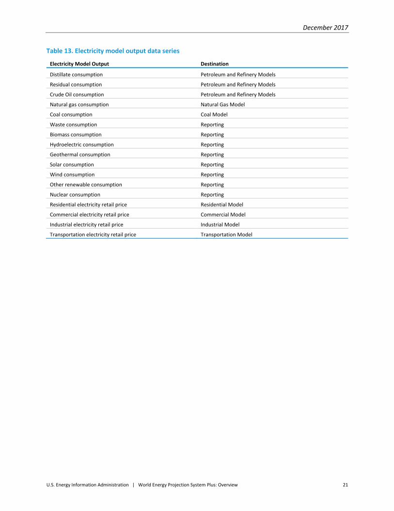
The Electricity Model projects consumption for a variety of energy sources and puts the projections into the common database for use by the other models. It also projects retail electricity prices for the demand sectors. (The model also writes generation and capacity projections to the common database, but they are not explicitly shown here.) These outputs are summarized in Table 13.

December 2017


Table 13. Electricity model output data series

Electricity Model Output Destination



Crude Oil consumption Petroleum and Refinery Models





Hydroelectric consumption Reporting


Solar consumption Reporting

Wind consumption Reporting

Other renewable consumption Reporting

Nuclear consumption Reporting

Residential electricity retail price Residential Model

Commercial electricity retail price Commercial Model

Industrial electricity retail price Industrial Model

Transportation electricity retail price Transportation Model

December 2017


9. District Heat Model

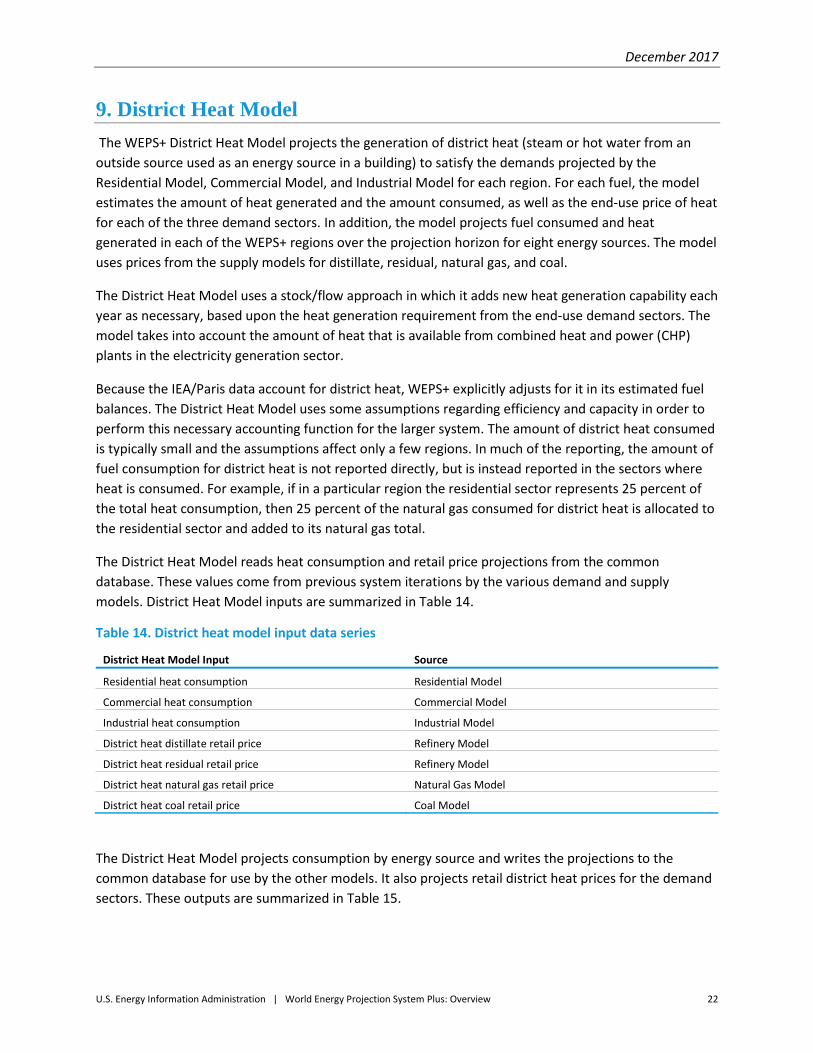
The WEPS+ District Heat Model projects the generation of district heat (steam or hot water from an

outside source used as an energy source in a building) to satisfy the demands projected by the

Residential Model, Commercial Model, and Industrial Model for each region. For each fuel, the model

estimates the amount of heat generated and the amount consumed, as well as the end-use price of heat

for each of the three demand sectors. In addition, the model projects fuel consumed and heat

generated in each of the WEPS+ regions over the projection horizon for eight energy sources. The model

uses prices from the supply models for distillate, residual, natural gas, and coal.

The District Heat Model uses a stock/flow approach in which it adds new heat generation capability each

year as necessary, based upon the heat generation requirement from the end-use demand sectors. The

model takes into account the amount of heat that is available from combined heat and power (CHP)

plants in the electricity generation sector.

Because the IEA/Paris data account for district heat, WEPS+ explicitly adjusts for it in its estimated fuel

balances. The District Heat Model uses some assumptions regarding efficiency and capacity in order to

perform this necessary accounting function for the larger system. The amount of district heat consumed

is typically small and the assumptions affect only a few regions. In much of the reporting, the amount of

fuel consumption for district heat is not reported directly, but is instead reported in the sectors where

heat is consumed. For example, if in a particular region the residential sector represents 25 percent of

the total heat consumption, then 25 percent of the natural gas consumed for district heat is allocated to

the residential sector and added to its natural gas total.

The District Heat Model reads heat consumption and retail price projections from the common

database. These values come from previous system iterations by the various demand and supply

models. District Heat Model inputs are summarized in Table 14.

Table 14. District heat model input data series

District Heat Model Input Source

Residential heat consumption Residential Model

Commercial heat consumption Commercial Model

Industrial heat consumption Industrial Model

District heat distillate retail price Refinery Model

District heat residual retail price Refinery Model

District heat natural gas retail price Natural Gas Model

District heat coal retail price Coal Model

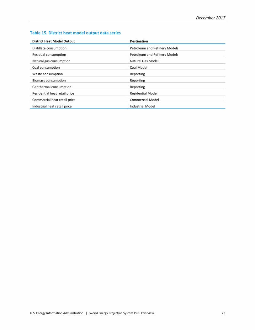
The District Heat Model projects consumption by energy source and writes the projections to the

common database for use by the other models. It also projects retail district heat prices for the demand

sectors. These outputs are summarized in Table 15.

December 2017


Table 15. District heat model output data series

District Heat Model Output Destination








Residential heat retail price Residential Model

Commercial heat retail price Commercial Model

Industrial heat retail price Industrial Model

December 2017


10. Petroleum Model

The WEPS+ Petroleum Model provides world oil prices to the WEPS+ system. World oil prices are

exogenously specified from an input file; the Petroleum Model accepts the price data and exports them

to the common database for use by other models. The model also has the capability of using an

algorithm in which supply elasticities can be used to change the world oil prices based on changes in

total world oil demand; however, this feedback capability is not generally used.

In order to estimate the sources and components of crude oil production given world oil prices, the

Petroleum Model must import total world crude oil demand projections. The WEPS+ system demand

estimates for crude oil are not modeled directly by the demand and transformation models in the

WEPS+ system but are implied indirectly through the demand for petroleum products and for petroleum

product substitutes in the various demand and transformation models. For example, a certain quantity

of crude oil will be required to meet the demand for motor gasoline in the transportation sector model.

The demand for products translates into a demand for crude oil through the refinery transformation

process. WEPS+ uses a two-part refinery model. The first part adds demand projections for petroleum

products across sectors and translates the demand for products and their substitutes into the total

world demand for crude oil. Thus the input to the Petroleum Model is the total world crude oil demand

read in from the common database (Table 16), which is projected by the first part of the Refinery Model.

Table 16. Petroleum model input data series

Petroleum Model Input Source

Total world crude oil demand Refinery Model (part 1)

The Petroleum Model projects the world oil price and writes it to the common database for subsequent

use by the Refinery Model (Table 17).

Table 17. Petroleum Model output data series

Petroleum Model Output Source

World oil price Refinery Model (part 2)

December 2017


11. Natural Gas Model

The WEPS+ Natural Gas Model projects wholesale natural gas prices for each of the sixteen regions. The

wholesale prices are then used to calculate retail prices using fixed sectoral markups. The retail prices

are written to the shared common database for use in the other demand and transformation models.

The Natural Gas Model is a reduced-form model that is estimated from perturbations of demand in the

separate, stand-alone International Natural Gas Model (INGM). This reduced-form model is a response-

surface type of model that starts with a base price at a base level of consumption, and then models

changes to the base price due to changes in the level of consumption. The base consumption, from a run

of the WEPS+ system, is provided to the INGM through an interface file. In turn, INGM provides base

price and reduced-form model coefficients to WEPS+, which then uses the reduced-form model for

subsequent runs, until there is a significant change.

The INGM1 is used to estimate the details of natural gas production, imports, exports, LNG, and other

supply components that are published in the IEO. In addition to the base price and consumption and the

reduced-form model coefficients, the INGM also passes some additional information at a regional level

to the Natural Gas Model. This includes natural gas production, natural gas liquids production, fuel

consumed in LNG operations, fuel consumed in gas-to-liquids (GTL) operations and as a feedstock,

production of oil by GTL operations, and reinjection. (Currently, pipeline use and lease and plant use are

determined in the INGM, but the Natural Gas Model makes its own separate forecast.) As the overall

demand levels change in WEPS+, these components of supply are adjusted or calibrated in fairly

straightforward algorithms by the Natural Gas Model. However, these algorithms and the components

of supply are currently being used as placeholders, and the actual published data is done in a

subsequent run of the INGM.

The key output of the Natural Gas Model is the wholesale price of natural gas in each region. Additional

regional markups are used in each region to allocate these wholesale prices to the retail price in each

demand sector. It is expected that this methodology will be enhanced in the future to directly account

for market relationships, subsidies, and taxes.

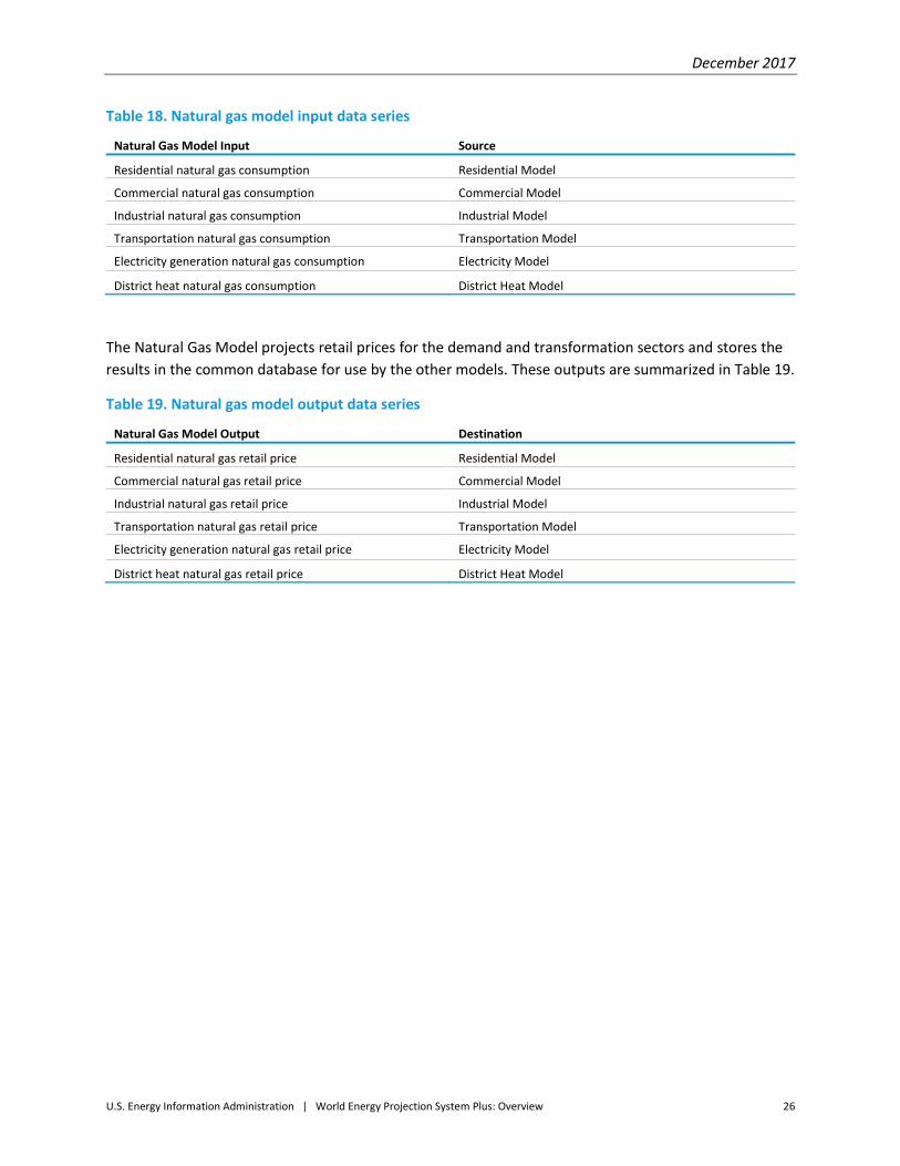
The Natural Gas Model reads natural gas consumption projections from the common database. These

values come from previous iterations by the various demand and transformation models. Natural Gas

Model inputs are summarized in Table 18.

1 A separate documentation report for the International Natural Gas Model (INGM) is available on the EIA web site.

December 2017


Table 18. Natural gas model input data series

Natural Gas Model Input Source

Residential natural gas consumption Residential Model

Commercial natural gas consumption Commercial Model

Industrial natural gas consumption Industrial Model

Transportation natural gas consumption Transportation Model

Electricity generation natural gas consumption Electricity Model

District heat natural gas consumption District Heat Model

The Natural Gas Model projects retail prices for the demand and transformation sectors and stores the

results in the common database for use by the other models. These outputs are summarized in Table 19.

Table 19. Natural gas model output data series

Natural Gas Model Output Destination

Residential natural gas retail price Residential Model

Commercial natural gas retail price Commercial Model

Industrial natural gas retail price Industrial Model

Transportation natural gas retail price Transportation Model

Electricity generation natural gas retail price Electricity Model

District heat natural gas retail price District Heat Model

December 2017


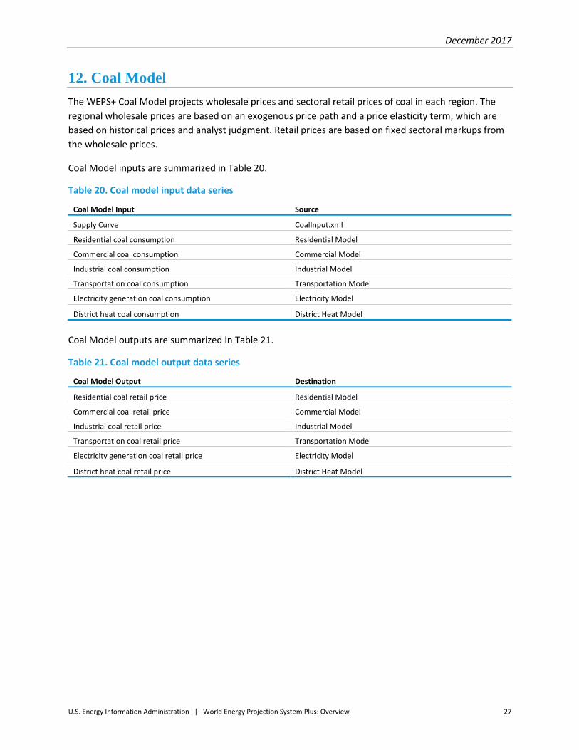
12. Coal Model

The WEPS+ Coal Model projects wholesale prices and sectoral retail prices of coal in each region. The

regional wholesale prices are based on an exogenous price path and a price elasticity term, which are

based on historical prices and analyst judgment. Retail prices are based on fixed sectoral markups from

the wholesale prices.

Coal Model inputs are summarized in Table 20.

Table 20. Coal model input data series

Coal Model Input Source

Supply Curve CoalInput.xml

Residential coal consumption Residential Model

Commercial coal consumption Commercial Model

Industrial coal consumption Industrial Model

Transportation coal consumption Transportation Model

Electricity generation coal consumption Electricity Model

District heat coal consumption District Heat Model

Coal Model outputs are summarized in Table 21.

Table 21. Coal model output data series

Coal Model Output Destination

Residential coal retail price Residential Model

Commercial coal retail price Commercial Model

Industrial coal retail price Industrial Model

Transportation coal retail price Transportation Model

Electricity generation coal retail price Electricity Model

District heat coal retail price District Heat Model

December 2017


13. Refinery Model

The WEPS+ Refinery Model has two main functions, and it is split into two separate models that run at

different points in the WEPS+ modeling stream. The first part runs before any of the other supply

models; its function is to determine the total amount of crude oil that needs to be produced. Part 1 adds

up the total petroleum products consumed by the demand and transformation models, and then

compares this data to the total amount of crude oil required. For example, the model accounts for the

amount of blends in motor gasoline, so that if a portion of the motor gasoline in a region is blended with

ethanol, then less motor gasoline product is required and less global crude oil production is required.

The model also accounts for amounts of oil that are produced in GTL operations. Ultimately, this first

part of the Refinery Model determines the amount of crude oil that needs to be produced and puts that

data into the common database for subsequent use by the Petroleum Model.

The second part of the Refinery Model runs after the supply models, and projects wholesale and retail

product prices. The Refinery Model is based on the concept of a “marginal” refinery and includes three

separate international specifications of a marginal refinery. These three specifications are for the U.S.

Gulf Coast, Northwest Europe, and Singapore. The marginal refinery model takes the world oil price as

specified by the Petroleum Model and then uses that, along with the petroleum product yields, to

determine the wholesale product prices that cover the crude and other costs for each refinery. These

local refinery prices are then allocated to each of the WEPS+ regions based on transportation costs and

transportation relationships. These regional wholesale product prices are then allocated to the demand

and transformation sectors based upon historical relationships. The retail prices are put into the

common database to be used by the other models.

The Refinery Model reads petroleum consumption projections from the common database. These

values come from previous iterations by the various demand and transformation models. Refinery

Model inputs are summarized in Table 22.

Table 22. Refinery model input data series

Refinery Model Input Source

World oil price Petroleum Model

Residential consumption of distillate, kerosene, and LPG Residential Model

Commercial consumption of motor gasoline, distillate, residual, kerosene, and LPG Commercial Model

Industrial consumption of motor gasoline, distillate, residual, kerosene, LPG, petroleum

coke, sequestered petroleum, other petroleum, and crude oil

Industrial Model

Transportation consumption of motor gasoline, distillate, residual, LPG, jet fuel,

sequestered petroleum, other petroleum, and crude oil

Transportation Model

Electricity generation consumption of distillate, residual, and crude oil Electricity Model

District heat consumption of distillate, residual, and crude oil District Heat Model

December 2017


The Refinery Model projects retail prices for the demand and transformation sectors, and exports them

to the common database for use by the other models. These outputs are summarized in Table 23.

Table 23. Refinery model output data series

Refinery Model Output Destination

Residential sector retail prices for distillate, kerosene, and LPG Residential Model

Commercial sector retail prices for motor gasoline, distillate, residual, kerosene, and LPG Commercial Model

Industrial sector retail prices for motor gasoline, distillate, residual, kerosene, and LPG Industrial Model

Transportation sector retail prices for motor gasoline, distillate, residual, LPG, jet fuel, other

petroleum, ethanol, and other biofuels

Transportation Model

Electricity sector generation retail prices for distillate and residual Electricity Model

District heat sector retail prices for distillate and residual District Heat Model

December 2017


14. Greenhouse Gases Model

The Greenhouse Gases Model projects energy-related carbon dioxide emissions by taking all of the

consumption projections of the other models from the common database and applying carbon dioxide

emissions factors to them. The emissions factors are calibrated to recent historical data from EIA’s

International Energy Statistics database. The model does not count emissions from fuel used as a

feedstock or “sequestered” or consumed in a carbon capture and storage technology. The model does

not address carbon dioxide emissions from non-energy consumption sources, nor does it account for

non-carbon dioxide greenhouse gas emissions.

December 2017


15. Main Model and Convergence Process

The primary objective of the WEPS+ Main Model is to evaluate and facilitate the convergence of the

modeling system. This process is at the heart of the interactive nature of the entire WEPS+ system and is

made possible by the way in which all the models communicate with each other to converge to an

overall equilibrium solution. Driving this process is the basic economic concept of dynamic markets using

prices to equilibrate demand and supply. In the modeling, the process is fairly straightforward for

individual relationships, but becomes quite elaborate when all the energy sources, sectors, and regions

are taken into account. The illustration in Figure 3, along with the discussion below, helps to explain the

convergence process.

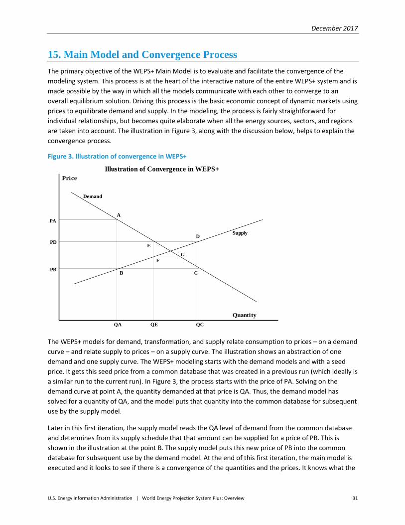
Figure 3. Illustration of convergence in WEPS+

The WEPS+ models for demand, transformation, and supply relate consumption to prices – on a demand

curve – and relate supply to prices – on a supply curve. The illustration shows an abstraction of one

demand and one supply curve. The WEPS+ modeling starts with the demand models and with a seed

price. It gets this seed price from a common database that was created in a previous run (which ideally is

a similar run to the current run). In Figure 3, the process starts with the price of PA. Solving on the

demand curve at point A, the quantity demanded at that price is QA. Thus, the demand model has

solved for a quantity of QA, and the model puts that quantity into the common database for subsequent

use by the supply model.

Later in this first iteration, the supply model reads the QA level of demand from the common database

and determines from its supply schedule that that amount can be supplied for a price of PB. This is

shown in the illustration at the point B. The supply model puts this new price of PB into the common

database for subsequent use by the demand model. At the end of this first iteration, the main model is

executed and it looks to see if there is a convergence of the quantities and the prices. It knows what the

A

PA

QA

BPB

C

QC

D

E

F

G

PD

QE

Demand

Supply

Price

Quantity

Illustration of Convergence in WEPS+

December 2017


quantities and prices were at the end of the previous iteration (or in this first iteration it knows what the

starting seed quantities and prices were). In the previous iteration, the quantity was QX (some unknown

value that is not illustrated above) and the price was PA. In the current iteration the quantity is QA, and

the price is PB. QX is probably not close to QA, and, as seen in the illustration above, PA is not close to

PB. Therefore, the system has not converged. The system will move to a new iteration and all the

models will be run again.

In the second iteration, the demand model reads the price PB from the common database (it was put

there by the supply model in the previous iteration). With the price of PB, the demand model

determines from its demand schedule that it demands the quantity QC (this is at the point C) and puts

that into the common database. Later in the second iteration, the supply model reads the QC level of

demand and determines from its supply schedule that it wants the price PD (this is at the point D) and

puts that into the common database. Again, at the end of this second iteration the Main Model is

executed and checks for convergence of quantities and prices. At the end of the previous iteration the

quantity was QA and the price was PB; now at the end of this iteration they are QC and PD, respectively.

The differences are now smaller than last time around but are still probably too large, so the system will

not have converged. The system will again move to a new iteration and all the models will be run again.

In the third iteration, much the same happens as demand moves to point E and supply moves to point F.

But, as can be seen in Figure 3, the differences between the starting points and the ending points for

consumption and prices are becoming much smaller. In the end, when the differences are less than the

convergence tolerance (which is set by the user), then the system will be close enough to the

equilibrium point and it will have “converged.” The iteration process stops when the system has

converged, and the system does whatever post-processing is necessary (typically report writing). A

detailed description of the three iteration steps is available in Table 24.

Table 24. Summary of the convergence process

Iteration 1

Demand Seed price of PA, solves at A for quantity QA

Supply Quantity QA, solves at B for price PB

Main Has not converged, continues iterations

Iteration 2

Demand Price PB, solves at C for quantity QC

Supply Quantity QC, solves at D for price PD

Main Compare QA to QC and PB to PD, not converged, continues iterations

Iteration 3

Demand Price PD, solves at E for quantity QE

Supply Quantity QE, solves at F for price PF (not shown)

Main Compare QC to QE and PD to PF, closer, at some point ending iterations

December 2017


The convergence process as described above is a simplification for illustration purposes. The actual

process in WEPS+ also includes a price “relaxation” (explained below) whenever the Main Model checks

for convergence. Price relaxation is done for two primary reasons. First, it is possible that the shapes of

the demand and supply curves are such that they do not converge and they actually diverge (this

depends upon the relative elasticity of each curve). Price relaxation makes this much more unlikely.

Second, price relaxation can greatly reduce the number of iterations and speed the movement to

convergence.

The model uses price relaxation when the system has not converged and is moving to the next iteration.

Instead of using the price from the current iteration to start the next iteration, the Main Model makes a

guess at the equilibrium price and instead puts this new price guess into the common database for use

in the next iteration. To understand price relaxation, it is helpful to consider the illustration above and

revisit the second iteration. From the end of the first iteration to the end of the second iteration, the

process has moved from point B to point C to point D, and the price has changed from PB to PD.

Ordinarily, the system would start the next iteration with the price PD in the common database. But

with price relaxation, instead of using the price PD, the Main Model makes a simple guess at the

equilibrium price by choosing the price midway between PB and PD. The original price PD, which the

supply model put into the common database, is replaced in the common database by the Main Model

with this alternative midpoint price. It can be clearly seen from the illustration that this simple midpoint

guess puts the price much closer to the equilibrium price. When the demand model is run in the next

iteration, this alternative price will cause the projected demand to be much closer to the equilibrium

demand. This simple price relaxation has greatly improved the convergence process.

There are several other simplifications in the illustration above. First, the system does not consist of one

single demand and supply schedule but instead considers a large number of energy sources in a number

of sectors in a variety of regions. Moreover, some of the demand and supply schedules may be

interrelated, and in some cases the supply schedule is an aggregate of many demands (for example,

solving for an overall regional natural gas wholesale price or solving for a worldwide world oil price).

Second, the actual convergence criteria in use are based on an overall weighted average rating, which

can be over several fuels or for a particular region or other aggregates. This is referred to as the

convergence “GPA;” the particulars for this and for the tolerance levels for the specific fuels and prices

are a user choice. Third, in each iteration, the models in WEPS+ are run for all years over the modeling

horizon. This makes it much easier to code the models, make the models more independent, and allow

them to be run as independent executables. This means that the convergence checking is done for all of

the years (or for some subset).

Documents

World Energy Projection System Plus: Overview · The World Energy Projection System Plus (WEPS+) is the energy modeling system used to produce the IEO2017. The complete WEPS+ system