Thank

Citatio

See th

Version

Copyri

Link to

you for do

on:

is record i

n:

ght Statem

o Published

wnloading

in the RMI

ment: ©

d Version:

this docum

IT Researc

ment from

ch Reposit

the RMIT R

ory at:

Research RRepository

PLEASE DO NOT REMOVE THIS PAGE

Date, A, Date, A and Akbarzadeh, A 2013, 'Investigating the potential for using a simplewater reaction turbine for power production from low head hydro resources', EnergyConversion and Management, vol. 66, pp. 257-270.

http://researchbank.rmit.edu.au/view/rmit:17983

Accepted Manuscript

2012 Elsevier

http://dx.doi.org/10.1016/j.enconman.2012.09.032

Investigating the potential of using simple reaction water

turbine for power production from low head hydro resources

Abhijit Date and Aliakbar Akbarzadeh

Energy CARE Group, School of Aerospace, Mechanical and Manufacturing Engineering,

RMIT University, PO Box 7 1, Bundoora, Victoria 3083, Australia

Abstract

In this analysis the simple reaction water turbine known as Barker's Mill is revisited. The

major geometrical and operational parameters have been identified and using principles

of conservation of mass, momentum and energy the governing equations have been

developed for the ideal case of zero frictional losses. The solutions of the resulting

equations are then offered in a non-dimensional form. It is shown that the maximum

torque produced by the machine is for the case when the turbine is stationary. At this

point the net output power is zero. As the load torque is decreased the turbine starts

rotating and power is produced. Furthermore, due to a centrifugal pumping effect, the

mass flow rate of water through the turbine increases during acceleration. Further

decrease in the load torque is accompanied by increase in speed, output power, water

mass flow rate and efficiency. It is shown that when the load torque is reduced towards

half the value of the torque at the stationary condition, then water mass flow rate, speed

and output power approach infinity. Under this condition the efficiency of the machine

approaches unity. The non-dimensional presentation of the characteristics of the idealized

turbine is used to investigate the characteristics of the machine and to explore its

application for production of power from water reservoirs of low heads. Theoretical

analysis of a simple reaction turbine considering the fluid frictional losses for practical

situation has been presented. A practical turbine will never runaway reach infinite speed

and the maximum power and efficiency of such turbine will only depend on the fluid

frictional losses. Here a new factor that represents the overall fluid frictional losses within

the turbine has been defined. Finally this paper briefly presents the experimental

performance results for two simple reaction water turbine prototypes. The two turbine

prototypes under investigation have different rotor diameters Ø0.24m and Ø0.12m. The

two turbine models were tested for the supply head ranging from 1m to 4m. The simple

reaction water turbine can operate under very low hydro-static head with high energy

conversion efficiency. This type of turbine exhibits prominent self-pumping ability at

high rotational speeds. Under low head to achieve high rotational speeds the turbine

diameter should be very small and this limits the volumetric capacity and hence the

power generation capacity of such a turbine. So the practical applications of this turbine

would be limited to the micro-hydro power generation. The split pipe design of the

reaction turbine is easy to manufacture and have proven to have energy conversion

efficiency of around 50% even under low heads.

Keywords: Simple Reaction Turbine; Water Turbine; Low Head Hydro; Hydro Electric.

Nomenclature

A Total nozzle exit area (m2)

D Nozzle diameter (m)

cD Nozzle equivalent diameter (m)

g Acceleration due to gravity (m/s2)

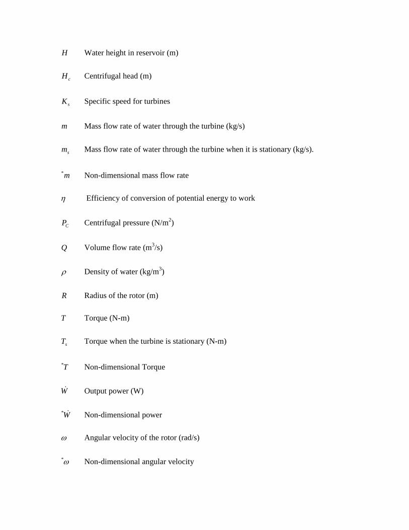
H Water height in reservoir (m)

cH Centrifugal head (m)

sK Specific speed for turbines

m Mass flow rate of water through the turbine (kg/s)

sm Mass flow rate of water through the turbine when it is stationary (kg/s).

m* Non-dimensional mass flow rate

η Efficiency of conversion of potential energy to work

CP Centrifugal pressure (N/m2)

Q Volume flow rate (m3/s)

ρ Density of water (kg/m3)

R Radius of the rotor (m)

T Torque (N-m)

sT Torque when the turbine is stationary (N-m)

T* Non-dimensional Torque

W Output power (W)

W* Non-dimensional power

ω Angular velocity of the rotor (rad/s)

ω* Non-dimensional angular velocity

U Tangential velocity of the nozzles (m/s)

U* Non-dimensional tangential velocity of the nozzles

aV Absolute velocity of water leaving the nozzle with respect to a stationary observer

(m/s)

aV* Non-dimensional absolute velocity

rV Relative velocity of water with respect to the nozzle (m/s)

rV* Non-dimensional relative velocity

Introduction

The use of moving water to drive machinery has a long history beginning with undershot

and overshot water wheels and progressing through turbines of various designs. Wilson

[1] provides an interesting brief history of water turbines to which the reader is referred.

Turbines are broadly classified into two types, impulse and reaction, although designs

may involve a mixture of the two types of action. In a pure impulse hydraulic turbine,

such as the Pelton wheel the energy associated with the pressure in the supply pipe is

converted to kinetic energy in the stationary nozzle (or vanes) and the high velocity

stream is directed onto moving buckets (or blades). There is no further change in pressure

of the water as it moves through the buckets and hence no change in the magnitude of the

velocity of the stream relative to the buckets. The buckets however change the direction

of the flow, and the movement of the buckets changes the magnitude of the stream's

absolute velocity. From the resulting change in momentum of the stream, the impulsive

force on the buckets and the torque on the wheel can be calculated. It is desirable, for

maximum energy extraction from the water that the wheel speed and bucket shape be

such that the water leaves the turbine with negligible kinetic energy[2, 3].

In a pure reaction hydraulic turbine the water is still pressurized as it enters the moving

parts and as it passes through the moving nozzles or vanes its pressure is reduced and the

velocity of the stream relative to the moving parts is increased. From the associated

change in absolute velocity and momentum, the reactive force and torque on the turbine

nozzle can be calculated. (Note that in the nozzle of the Pelton wheel a reaction force is

also generated, but since the nozzle is stationary no mechanical energy is extracted at that

point.) The earliest recorded reaction turbine, that of Hero (about 2,000 years ago) [4]

was a reaction machine and is illustrated in Fig. 1, some experiments of the modem day

Hero type turbines are described by Hsu and Leo [5]and Brady [6]. Barker's mill, which

is shown diagrammatically in Fig. 2, was the first hydraulic reaction turbine and was

invented in about 1740, this machine was further refined by Pupil in 1775 and Whitelaw

in 1839 [1]. One such refinement is to feed the water into the underside of the rotor. By

feeding water into the turbine from underneath as shown in Fig. 3 the upward action of

the static pressure of the entering feed water may be used to counteract the downward

gravitational force on the moving parts thereby reducing the thrust load on bearings

supporting these moving parts.

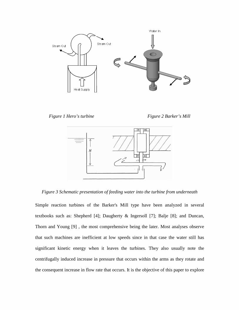
Figure 1 Hero’s turbine Figure 2 Barker’s Mill

Figure 3 Schematic presentation of feeding water into the turbine from underneath

Simple reaction turbines of the Barker's Mill type have been analyzed in several

textbooks such as: Shepherd [4]; Daugherty & Ingersoll [7]; Balje [8]; and Duncan,

Thorn and Young [9] , the most comprehensive being the later. Most analyses observe

that such machines are inefficient at low speeds since in that case the water still has

significant kinetic energy when it leaves the turbines. They also usually note the

centrifugally induced increase in pressure that occurs within the arms as they rotate and

the consequent increase in flow rate that occurs. It is the objective of this paper to explore

in more detail the changes in efficiency, flow rate, torque and power that occur with

increase in speed of rotation of an ideal frictionless Barker's Mill.

Through parametric analysis, attempts are also made to undertake a comprehensive study

on the characteristics of the frictionless simple reaction water turbine and present its

inherent potential as a candidate for application to low head water reservoirs for the

production of power. As part of the discussions presented in this work, what the authors

believe to be incorrect conclusions, which have been drawn in the published literature,

will be pointed out. The conclusions relate to the performance of simple reaction water

turbines as their speed tends towards infinity.

In short, it appears that simple reaction water turbines are to some extent misunderstood,

under-utilized and almost forgotten other than for garden sprinklers. The aim of this

paper is to demonstrate the main features of these devices and to propose potential

application to renewable electrical power generation.

Theoretical analysis of idealized simple reaction turbine

In this section attempts are made to provide governing equations for prediction of the

performance of a simple reaction water turbine. These equations are then used for

parametric study of the performance of the machine under specified conditions.

Let us assume that total head of H (m) is available in a water reservoir and the aim is to

convert the potential energy of water to useful work by the means of a simple reaction

turbine as shown in Fig 3.

Here we neglect all losses due to friction such as losses due to the flow of water from the

reservoir, and through the piping, the rotor and the nozzles. We also neglect all the other

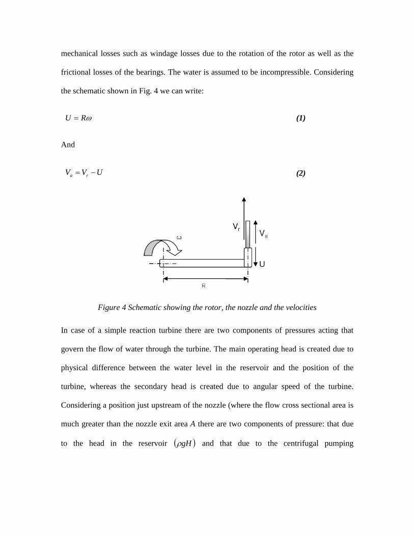
mechanical losses such as windage losses due to the rotation of the rotor as well as the

frictional losses of the bearings. The water is assumed to be incompressible. Considering

the schematic shown in Fig. 4 we can write:

ωRU = (1)

And

UVV ra −= (2)

Figure 4 Schematic showing the rotor, the nozzle and the velocities

In case of a simple reaction turbine there are two components of pressures acting that

govern the flow of water through the turbine. The main operating head is created due to

physical difference between the water level in the reservoir and the position of the

turbine, whereas the secondary head is created due to angular speed of the turbine.

Considering a position just upstream of the nozzle (where the flow cross sectional area is

much greater than the nozzle exit area A there are two components of pressure: that due

to the head in the reservoir ( )gHρ and that due to the centrifugal pumping

action ( )22

21 RPc ρω= . The combined effect of these pressures is to drive the water out

at a velocity relative to the nozzle found from:

222

21

21 RgHVr ρωρρ += (3)

Alternatively it can be rewritten as:

( )cr HHgV += ρρ 2

21 (4)

Where the centrifugal head,

gRHc 2

22ω= (5)

From Eq.(3):

222 RgHVr ω+= (6)

Mass flow out of the nozzle may be found from:

AVm rρ=•

(7)

Where,

( )222 RgHAm ωρ += (8)

By consideration of Eq. (8) it can be seen that the mass flow is at a minimum when the

turbine is stationary and increases as the turbine angular velocity increases. This self

pumping effect is mentioned qualitatively by J.R. Ainsworth Davis [10]. This centrifugal

head or self-pumping phenomenon is similar to working principle of a centrifugal pump.

The minimum value which occurs when the turbine is stationary we have called,

gHAms 2ρ=•

(9)

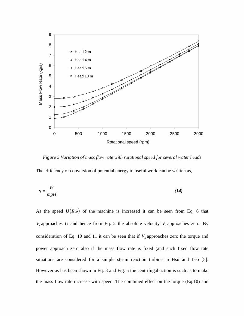
Fig. 5 shows mass flow rate of water as a function of rotational speed for several different

heads applied to a machine for which 24102 mA −×= and mR 125.0= .

Momentum balance results in,

RVmT a

•

= (10)

The produced power can be related to torque T and angular velocity ω in the following

form

ωTW = (11)

Using conservation of energy we also obtain, assuming, as stated earlier, no frictional

losses:

2

21

aVmwgHm += (12)

Where,

2

21

aVmgHmW += (13)

0

1

2

3

4

5

6

7

8

9

0 500 1000 1500 2000 2500 3000

Rotational speed (rpm)

Mas

s Fl

ow R

ate

(kg/

s)

Head 2 m

Head 4 m

Head 5 m

Head 10 m

Figure 5 Variation of mass flow rate with rotational speed for several water heads

The efficiency of conversion of potential energy to useful work can be written as,

gHmW

=η (14)

As the speed U ( )ωR of the machine is increased it can be seen from Eq. 6 that

rV approaches U and hence from Eq. 2 the absolute velocity aV approaches zero. By

consideration of Eq. 10 and 11 it can be seen that if aV approaches zero the torque and

power approach zero also if the mass flow rate is fixed (and such fixed flow rate

situations are considered for a simple steam reaction turbine in Hsu and Leo [5].

However as has been shown in Eq. 8 and Fig. 5 the centrifugal action is such as to make

the mass flow rate increase with speed. The combined effect on the torque (Eq.10) and

power (Eq.11) of these two opposing trends of decreasing aV versus increasing m is not

immediately apparent, and is explored subsequently in this paper. Duncan [9] state that

when RVr ω= the power is zero, but do not explore the aforementioned combined effect

on power of m approaching infinity as rV and Rω approach each other at high speed.

Similarly Daugherty [7] associate the runaway high speed condition with zero torque due

to the absolute fluid velocity approaching zero without considering the opposing trend of

mass flow approaching infinity. Duncan [9] however discuss the tendency towards

instability of the outward flow turbine. Instability in this context is the characteristic of

having a self enhancing runaway tendency if the torque is reduced. By contrast, inward

flowing turbines such as the Thomson and Francis are self governing to some extent in

that a speeding up causes a build up of centrifugal pressure that tends to reduce the

inward mass flow and hence the torque.

In the above equations R, A and H are known geometrical parameters, ρ is the density of

water and g is the acceleration due to gravity. Here the solutions of the above algebraic

equations are offered based on the load torque T. By solving equations (1) to (14) the

equations relating the seven unknowns i.e., WmVVU ra ,,,,, ω and η to the known

parameters of the system can be developed.

We have chosen to offer the solutions in a particular non-dimensional form for ease of

presentation and generalization of the results. As found in Eq. 9, sm is the mass flow rate

through the turbine when the turbine is stationary.

This mass flow rate causes a reaction, which needs to be balanced by sT which is given

by:

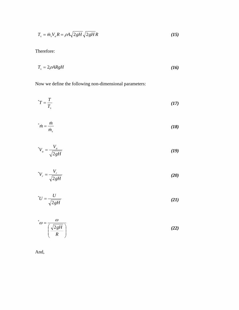
RgHgHARVmT ass 22ρ== (15)

Therefore:

ARgHTs ρ2= (16)

Now we define the following non-dimensional parameters:

sTTT =* (17)

smmm

=* (18)

gHV

V aa 2

* = (19)

gHVV r

r 2* = (20)

gHUU2

* = (21)

=

RgH2

* ωω (22)

And,

gHmWWs

=* (23)

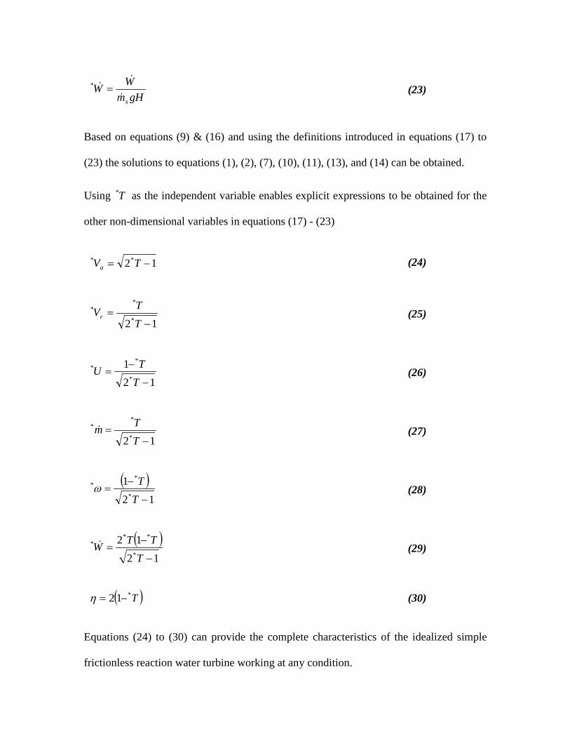
Based on equations (9) & (16) and using the definitions introduced in equations (17) to

(23) the solutions to equations (1), (2), (7), (10), (11), (13), and (14) can be obtained.

Using T* as the independent variable enables explicit expressions to be obtained for the

other non-dimensional variables in equations (17) - (23)

12** −= TVa (24)

12*

**

−=

TTVr (25)

121

*

**

−

−=

TTU (26)

12*

**

−=

TTm (27)

( )12

1*

**

−

−=

TTω (28)

( )12

12*

***

−

−=

TTTW (29)

( )T*12 −=η (30)

Equations (24) to (30) can provide the complete characteristics of the idealized simple

frictionless reaction water turbine working at any condition.

The universal characteristics of this turbine are presented graphically in Fig. 6 using the

dimensionless torque T* as the independent variable. Reducing the load torque applied to

the machine from the stationary to runaway condition corresponds to moving from right

to left on the horizontal axis.

Fig. 7 shows η,,,, **** WTmVa presented as a function of ω* . Although presented as a

function of ω* the values shown were generated from equations (24) to (30) by

varying T* . Equations (24)- (30), along with the graphical presentation in Fig.6 and Fig.

7, offers the complete set of information in a universal form for the analysis of simple

ideal outward flowing reaction water turbines.

Discussion of ideal performance curves

At the right hand end of the graphs in Fig. 6 the turbine is stationary and, as has already

been discussed the mass flow rate through the turbine has its least value when the

machine is not rotating. At this point the stationary torque sT given by Eq. 16 needs to be

applied to balance the torque from the reaction to the flow of water sm through the

nozzles given by Eq. 9. At this point the value of non-dimensional torque T* defined in

Eq. 17 is equal to one (i.e. 1* =T ). Since the machine is stationary i.e. ω* = 0, no power

is produced ( W* = 0) and efficiency η = 0. Furthermore aV is at its maximum ( aV* =l).

0

0.5

1

1.5

2

2.5

3

3.5

4

4.5

5

0.5 0.6 0.7 0.8 0.9 1*T

*Va

*m

*ω

*W

*η

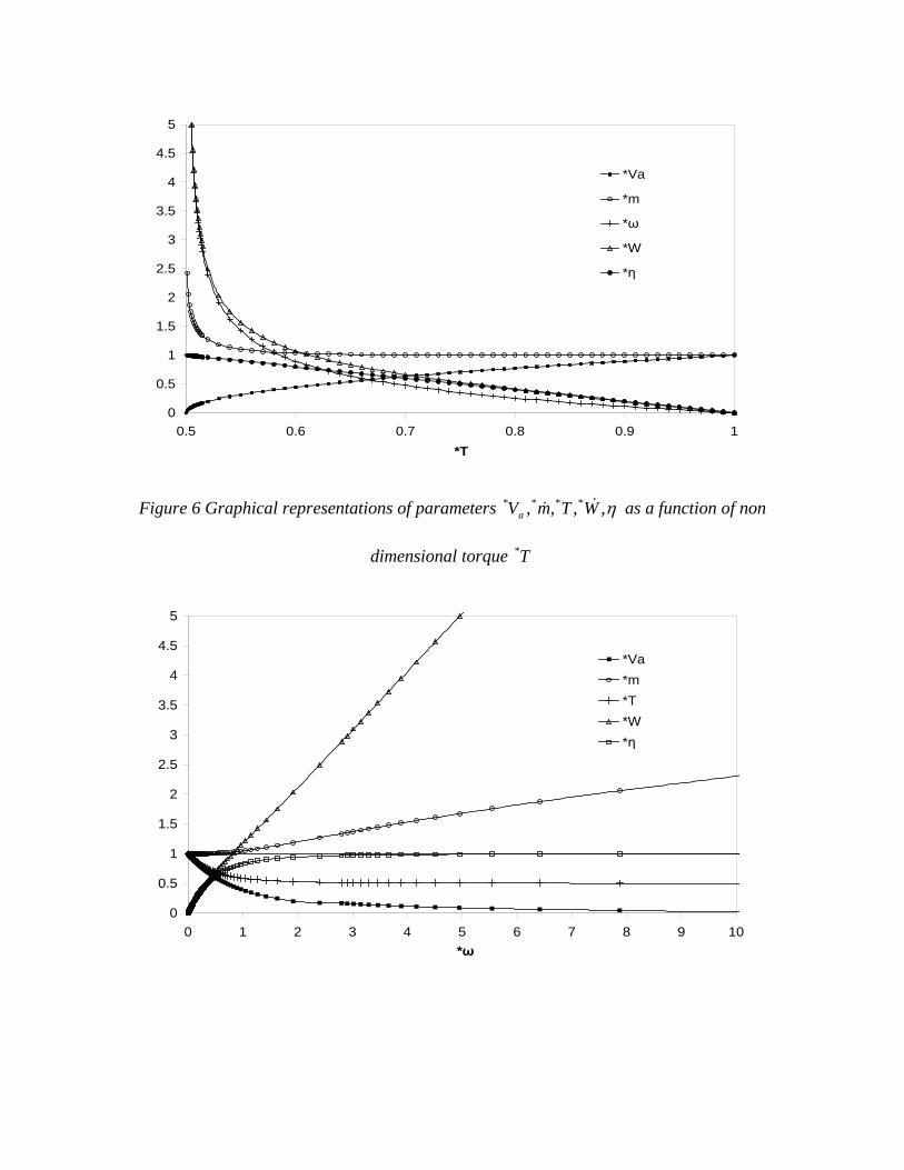
Figure 6 Graphical representations of parameters η,,,, **** WTmVa as a function of non

dimensional torque T*

0

0.5

1

1.5

2

2.5

3

3.5

4

4.5

5

0 1 2 3 4 5 6 7 8 9 10*ω

*Va*m*T*W*η

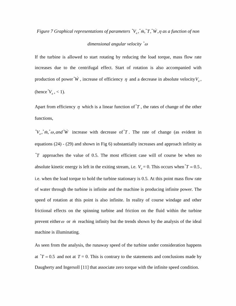
Figure 7 Graphical representations of parameters η,,,, **** WTmVa as a function of non

dimensional angular velocity ω*

If the turbine is allowed to start rotating by reducing the load torque, mass flow rate

increases due to the centrifugal effect. Start of rotation is also accompanied with

production of power W* , increase of efficiency η and a decrease in absolute velocity aV ,

(hence aV* , < 1).

Apart from efficiency η which is a linear function of T* , the rates of change of the other

functions,

WandmVa **** ,,, ω increase with decrease of T* . The rate of change (as evident in

equations (24) - (29) and shown in Fig 6) substantially increases and approach infinity as

T* approaches the value of 0.5. The most efficient case will of course be when no

absolute kinetic energy is left in the exiting stream, i.e. aV = 0. This occurs when 5.0* =T ,

i.e. when the load torque to hold the turbine stationary is 0.5. At this point mass flow rate

of water through the turbine is infinite and the machine is producing infinite power. The

speed of rotation at this point is also infinite. In reality of course windage and other

frictional effects on the spinning turbine and friction on the fluid within the turbine

prevent eitherω or m reaching infinity but the trends shown by the analysis of the ideal

machine is illuminating.

As seen from the analysis, the runaway speed of the turbine under consideration happens

at 5.0* =T and not at T = 0. This is contrary to the statements and conclusions made by

Daugherty and Ingersoll [11] that associate zero torque with the infinite speed condition.

Behavior of the turbine as T* approaches 0.5: Under this condition the behavior of the

three variables ω** ,m and W* is interesting. Considering the equations (27), (28) and (29)

these three functions approach infinity with closely similar values. As a numerical

example at T* = 0.501 we have m* = 11.203, ω* = 11.158 and W* = 11.180 as calculated

from the corresponding equations. At this point aV* = 0.045 and =η 0.998.

At T* = 0.5001 the values of Wm *** ,, ω are 35.362, 35.348 and 35.355 respectively. At

this point aV* = 0.0014 and η = 1.000.

Discussion of the general characteristics

Based on the analysis presented in the previous discussions it is seen that the idealized

simple reaction water turbine is more efficient the faster it turns. Moreover, the

centrifugal effect which pushes more water through the turbine results in an increase in

the power producing capacity of the machine. This can possibly be important as it may

enable production of compact water turbine of small sizes. Also the fact that the above

machine achieves its highest efficiency at high speeds can also result in smaller and more

compact electrical generators. Since the machine increases its volume throughput by

using the centrifugal pumping effect, this may mean that the simple ideal reaction water

turbine could offer a solution for power production from water reservoirs of low head

which may not be suitable to be utilized by conventional water turbines operating on the

impulse principal. The runaway potential at low loads however must be recognized. More

sophisticated inward flowing reaction turbine types such as the Thomson and Francis

have some self-governing effect in that high speeds of rotation cause an increase of

centrifugal pressure that opposes the inward flow.

Example

Here through some numerical examples some of the points made above are demonstrated.

Assume the rotor diameter to be 0.25m having two nozzles each having an exit opening

of l0mm x 10mm. This results in total nozzle exit area A of 2x10-4m2. The density of

water is assumed to be ρ = 1000 kg/m3 and acceleration of gravity g = 9.81m/s2. The

characteristics of such a rotor i.e. torque, power and efficiency are presented in Fig. 8 to

Fig. 10 as functions of rotational speed for four different heads namely lm, 2m, 5m and

10m. This is the range of water heads which are considered to be more suitable for simple

reaction water turbines. It is in this range that it is believed at this stage that the above

turbine has its most applications.

As shown previously, Fig. 5 presents the variation of water flow rate versus rotational

speed. It is observed that for the same head, flow rate increases with rotational speed. The

rate of increase is initially low, but it increases at higher rotational speeds and eventually

assumes a linear variation. It is interesting to note that the effect of the head on water

flow rate diminishes at higher speeds. This is due to the self-pumping phenomenon,

which is as explained before, one of the main features of the machine under discussion.

From the graphs in Fig. 5 it is evident that the curves relating to different heads become

closer and follow an asymptote as rotational speeds increases.

Fig. 8 shows the variation of shaft torque versus rotational speed. As seen for all four

heads the maximum torque is produced when the machine is not rotating. The rotation of

the machine is accompanied with a drop in the produced torque. The torque is decreased

further as speed increases approaching asymptotically half the value of the starting

torque.

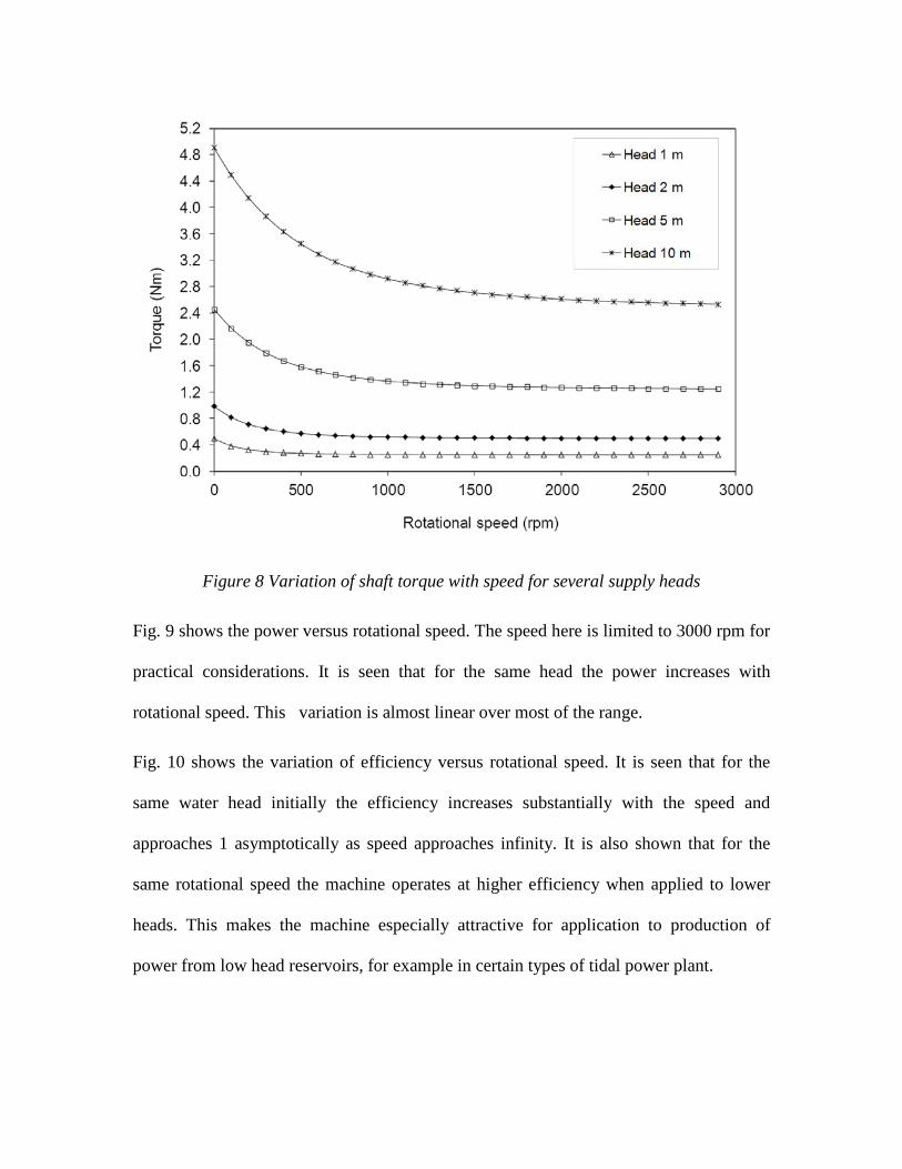
Figure 8 Variation of shaft torque with speed for several supply heads

Fig. 9 shows the power versus rotational speed. The speed here is limited to 3000 rpm for

practical considerations. It is seen that for the same head the power increases with

rotational speed. This variation is almost linear over most of the range.

Fig. 10 shows the variation of efficiency versus rotational speed. It is seen that for the

same water head initially the efficiency increases substantially with the speed and

approaches 1 asymptotically as speed approaches infinity. It is also shown that for the

same rotational speed the machine operates at higher efficiency when applied to lower

heads. This makes the machine especially attractive for application to production of

power from low head reservoirs, for example in certain types of tidal power plant.

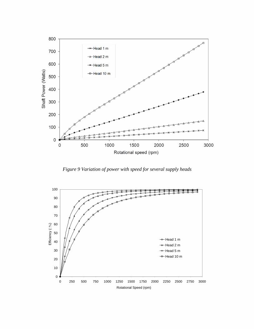
Figure 9 Variation of power with speed for several supply heads

0

10

20

30

40

50

60

70

80

90

100

0 250 500 750 1000 1250 1500 1750 2000 2250 2500 2750 3000

Rotational Speed (rpm)

Effi

cien

cy ( h

%)

Head 1 mHead 2 mHead 5 mHead 10 m

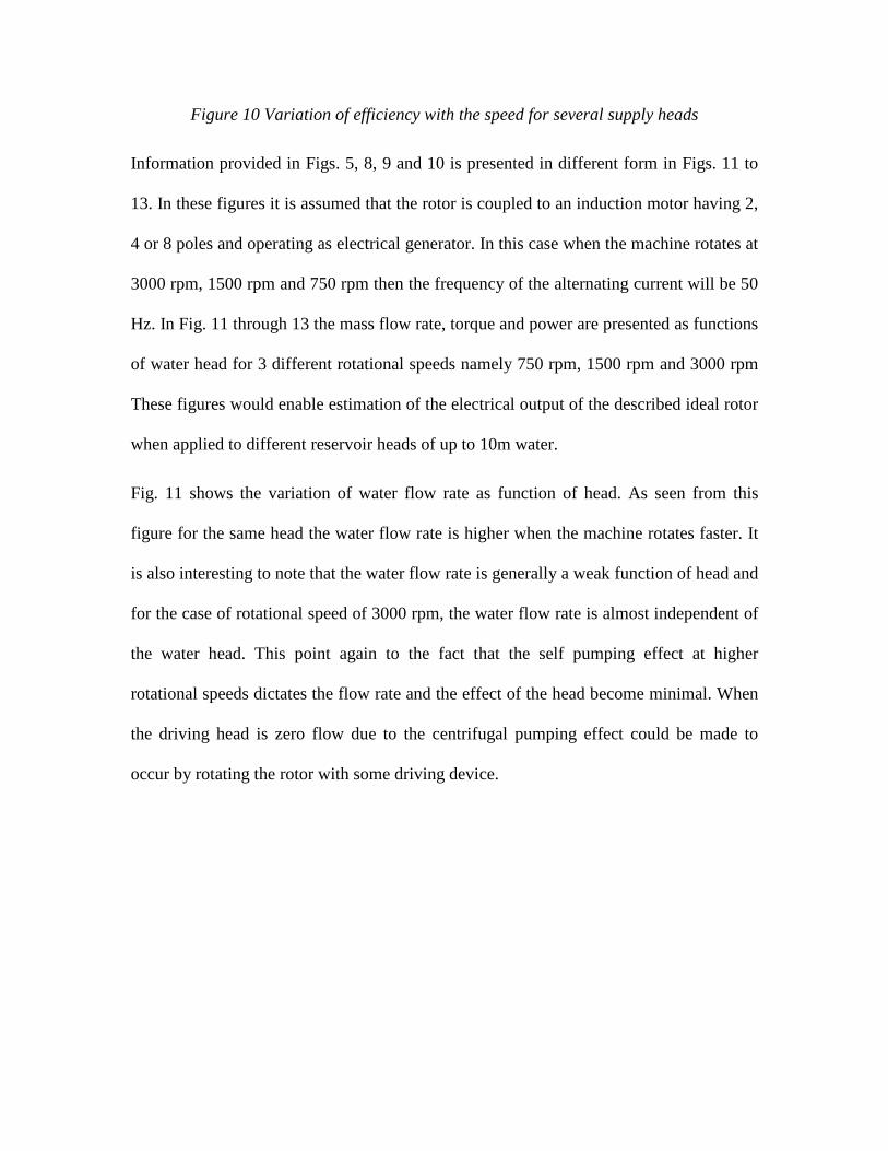
Figure 10 Variation of efficiency with the speed for several supply heads

Information provided in Figs. 5, 8, 9 and 10 is presented in different form in Figs. 11 to

13. In these figures it is assumed that the rotor is coupled to an induction motor having 2,

4 or 8 poles and operating as electrical generator. In this case when the machine rotates at

3000 rpm, 1500 rpm and 750 rpm then the frequency of the alternating current will be 50

Hz. In Fig. 11 through 13 the mass flow rate, torque and power are presented as functions

of water head for 3 different rotational speeds namely 750 rpm, 1500 rpm and 3000 rpm

These figures would enable estimation of the electrical output of the described ideal rotor

when applied to different reservoir heads of up to 10m water.

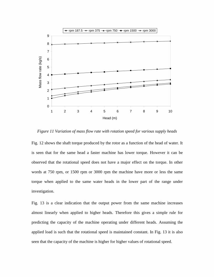
Fig. 11 shows the variation of water flow rate as function of head. As seen from this

figure for the same head the water flow rate is higher when the machine rotates faster. It

is also interesting to note that the water flow rate is generally a weak function of head and

for the case of rotational speed of 3000 rpm, the water flow rate is almost independent of

the water head. This point again to the fact that the self pumping effect at higher

rotational speeds dictates the flow rate and the effect of the head become minimal. When

the driving head is zero flow due to the centrifugal pumping effect could be made to

occur by rotating the rotor with some driving device.

0

1

2

3

4

5

6

7

8

9

1 2 3 4 5 6 7 8 9 10

Head (m)

Mas

s flo

w ra

te (k

g/s)

rpm 187.5 rpm 375 rpm 750 rpm 1500 rpm 3000

Figure 11 Variation of mass flow rate with rotation speed for various supply heads

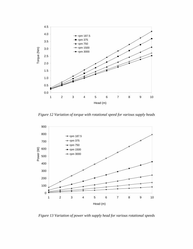
Fig. 12 shows the shaft torque produced by the rotor as a function of the head of water. It

is seen that for the same head a faster machine has lower torque. However it can be

observed that the rotational speed does not have a major effect on the torque. In other

words at 750 rpm, or 1500 rpm or 3000 rpm the machine have more or less the same

torque when applied to the same water heads in the lower part of the range under

investigation.

Fig. 13 is a clear indication that the output power from the same machine increases

almost linearly when applied to higher heads. Therefore this gives a simple rule for

predicting the capacity of the machine operating under different heads. Assuming the

applied load is such that the rotational speed is maintained constant. In Fig. 13 it is also

seen that the capacity of the machine is higher for higher values of rotational speed.

0.0

0.5

1.0

1.5

2.0

2.5

3.0

3.5

4.0

4.5

1 2 3 4 5 6 7 8 9 10

Head (m)

Torq

ue (N

m)

rpm 187.5rpm 375rpm 750rpm 1500rpm 3000

Figure 12 Variation of torque with rotational speed for various supply heads

0

100

200

300

400

500

600

700

800

900

1 2 3 4 5 6 7 8 9 10

Head (m)

Pow

er (W

)

rpm 187.5

rpm 375

rpm 750

rpm 1500

rpm 3000

Figure 13 Variation of power with supply head for various rotational speeds

Simple reaction turbine and specific speed

Specific speeds are commonly used as a tool for comparison of the characteristics of

similar hydraulic machines. Here this tool is applied to simple reaction water turbine, by

using the formulation provided by Turton [12] for the specific speed of turbines, the

following relation between specific speed and efficiency of a simple reaction turbine has

been derived.

( ) 43

43

1

22

η

ηη

−

−××=

−

RAK s

(31)

The effect of geometry on the relation between specific speed and efficiency is expressed

in terms of RA . However this can be changed to ratio of diameters i.e. dD where

RD 2= and d is the diameter of the nozzle. Defining an equivalent exit nozzle diameter

ed as,

Ad e ×Π

=2 (32)

Using the relation for the equivalent exit nozzle diameter from equation (2), we can re-

write equation (1) as follows,

( ) 43

43

1

22η

ηη

−

−××Π×=

−

DdK e

s (33)

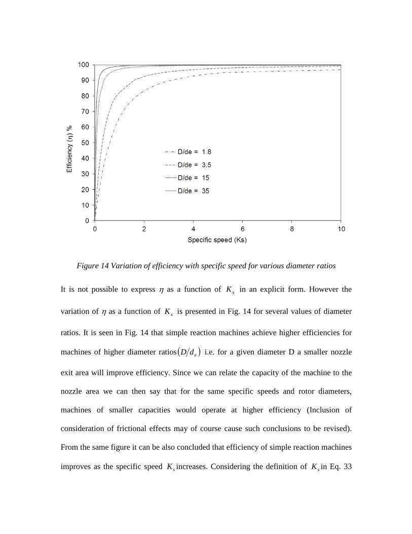
Figure 14 Variation of efficiency with specific speed for various diameter ratios

It is not possible to express η as a function of sK in an explicit form. However the

variation of η as a function of sK is presented in Fig. 14 for several values of diameter

ratios. It is seen in Fig. 14 that simple reaction machines achieve higher efficiencies for

machines of higher diameter ratios ( )edD i.e. for a given diameter D a smaller nozzle

exit area will improve efficiency. Since we can relate the capacity of the machine to the

nozzle area we can then say that for the same specific speeds and rotor diameters,

machines of smaller capacities would operate at higher efficiency (Inclusion of

consideration of frictional effects may of course cause such conclusions to be revised).

From the same figure it can be also concluded that efficiency of simple reaction machines

improves as the specific speed sK increases. Considering the definition of sK in Eq. 33

this is equivalent to saying high efficiencies are achieved at high speeds, high volume

flow rate and low heads. This can be considered an important conclusion in relation to the

characteristics of simple reaction water turbines.

Analysis of simple reaction water turbine for practical operating condition with

losses

Now if we consider real operating condition there would be considerable amount of

losses associated with the flow of water through the simple reaction water turbine. In this

section a factor that would represent the losses associated with the fluid flow through the

turbine has been defined, this factor would be called as k-factor throughout this paper.

For a practical situation the energy balance equation would be different than that in an

ideal situation, as there would be some energy lost due to fluid friction within the turbine

and a majority at the exit nozzles due to the high velocity of exiting water jets. So in this

situation the energy balance equation would be written as follows,

22

21

21

ra kVmVmWgHm ++= (34)

Here, 2

21

rkVm represents the fluid frictional losses associated with the flow of water

through the turbine exit nozzles, 2

21

aVm represents the loss of kinetic energy with the

water leaving the turbine, W represents the shaft power and gHm is the rate of potential

energy supplied to the turbine. So with increase in the value of k-factor the shaft power

would decrease and this is obvious from the following equation,

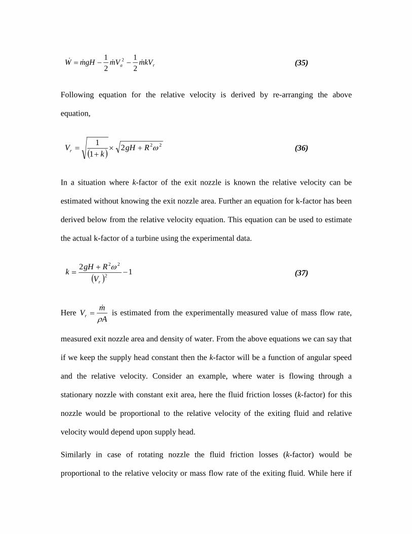
ra kVmVmgHmW 21

21 2 −−= (35)

Following equation for the relative velocity is derived by re-arranging the above

equation,

( )222

11 ωRgH

kVr +×

+= (36)

In a situation where k-factor of the exit nozzle is known the relative velocity can be

estimated without knowing the exit nozzle area. Further an equation for k-factor has been

derived below from the relative velocity equation. This equation can be used to estimate

the actual k-factor of a turbine using the experimental data.

( )12

2

22

−+

=rV

RgHk ω (37)

Here A

mVr ρ

= is estimated from the experimentally measured value of mass flow rate,

measured exit nozzle area and density of water. From the above equations we can say that

if we keep the supply head constant then the k-factor will be a function of angular speed

and the relative velocity. Consider an example, where water is flowing through a

stationary nozzle with constant exit area, here the fluid friction losses (k-factor) for this

nozzle would be proportional to the relative velocity of the exiting fluid and relative

velocity would depend upon supply head.

Similarly in case of rotating nozzle the fluid friction losses (k-factor) would be

proportional to the relative velocity or mass flow rate of the exiting fluid. While here if

the turbine is rotating then the relative velocity / mass flow rate would change with

change in angular speed due to centrifugal pumping effect discussed earlier.

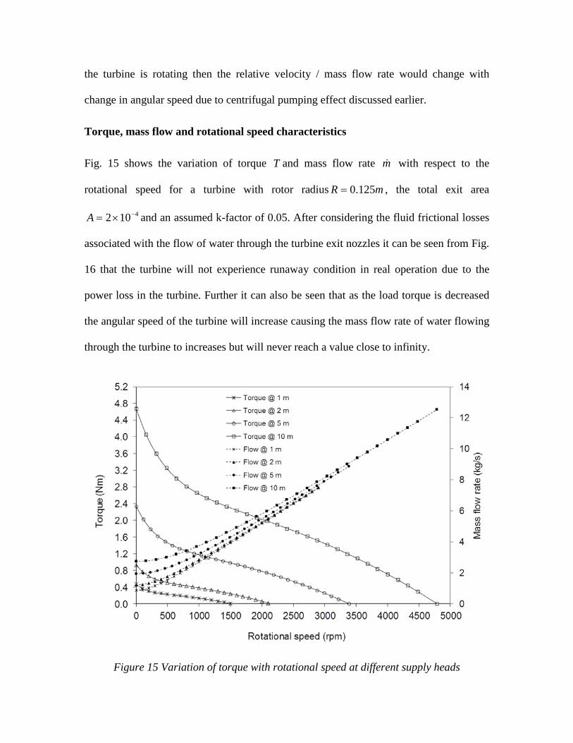
Torque, mass flow and rotational speed characteristics

Fig. 15 shows the variation of torque T and mass flow rate m with respect to the

rotational speed for a turbine with rotor radius mR 125.0= , the total exit area

4102 −×=A and an assumed k-factor of 0.05. After considering the fluid frictional losses

associated with the flow of water through the turbine exit nozzles it can be seen from Fig.

16 that the turbine will not experience runaway condition in real operation due to the

power loss in the turbine. Further it can also be seen that as the load torque is decreased

the angular speed of the turbine will increase causing the mass flow rate of water flowing

through the turbine to increases but will never reach a value close to infinity.

Figure 15 Variation of torque with rotational speed at different supply heads

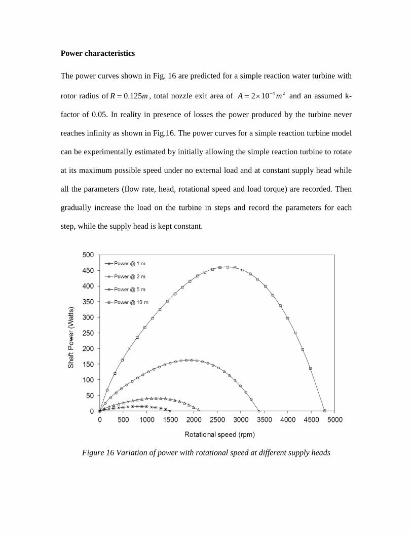
Power characteristics

The power curves shown in Fig. 16 are predicted for a simple reaction water turbine with

rotor radius of mR 125.0= , total nozzle exit area of 24102 mA −×= and an assumed k-

factor of 0.05. In reality in presence of losses the power produced by the turbine never

reaches infinity as shown in Fig.16. The power curves for a simple reaction turbine model

can be experimentally estimated by initially allowing the simple reaction turbine to rotate

at its maximum possible speed under no external load and at constant supply head while

all the parameters (flow rate, head, rotational speed and load torque) are recorded. Then

gradually increase the load on the turbine in steps and record the parameters for each

step, while the supply head is kept constant.

Figure 16 Variation of power with rotational speed at different supply heads

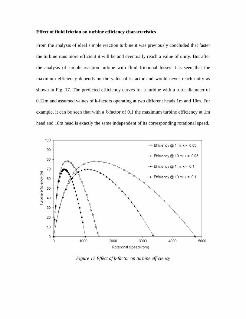
Effect of fluid friction on turbine efficiency characteristics

From the analysis of ideal simple reaction turbine it was previously concluded that faster

the turbine runs more efficient it will be and eventually reach a value of unity. But after

the analysis of simple reaction turbine with fluid frictional losses it is seen that the

maximum efficiency depends on the value of k-factor and would never reach unity as

shown in Fig. 17. The predicted efficiency curves for a turbine with a rotor diameter of

0.12m and assumed values of k-factors operating at two different heads 1m and 10m. For

example, it can be seen that with a k-factor of 0.1 the maximum turbine efficiency at 1m

head and 10m head is exactly the same independent of its corresponding rotational speed.

Figure 17 Effect of k-factor on turbine efficiency

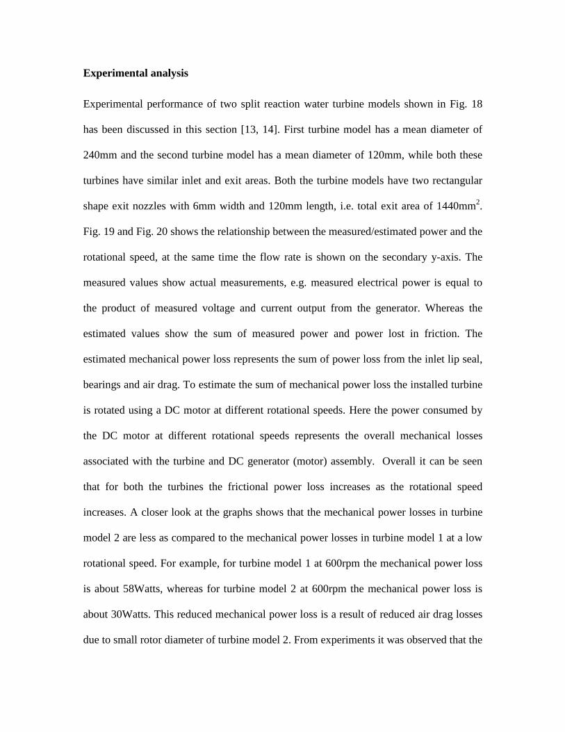
Experimental analysis

Experimental performance of two split reaction water turbine models shown in Fig. 18

has been discussed in this section [13, 14]. First turbine model has a mean diameter of

240mm and the second turbine model has a mean diameter of 120mm, while both these

turbines have similar inlet and exit areas. Both the turbine models have two rectangular

shape exit nozzles with 6mm width and 120mm length, i.e. total exit area of 1440mm2.

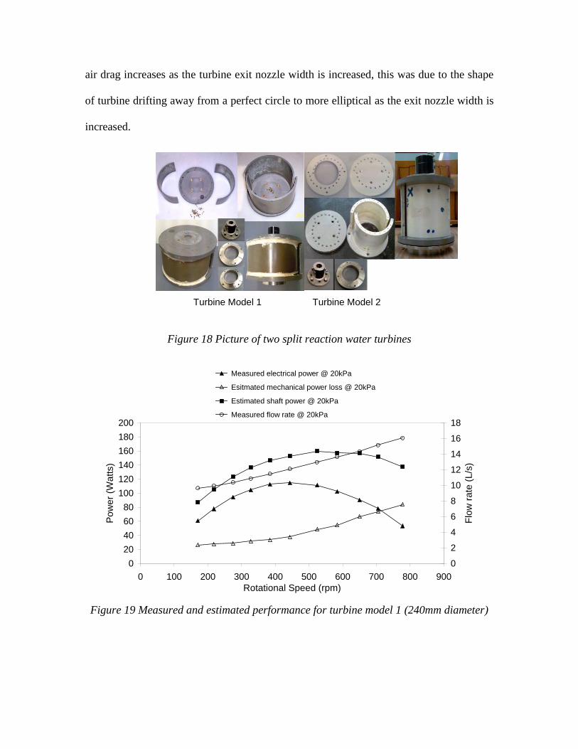
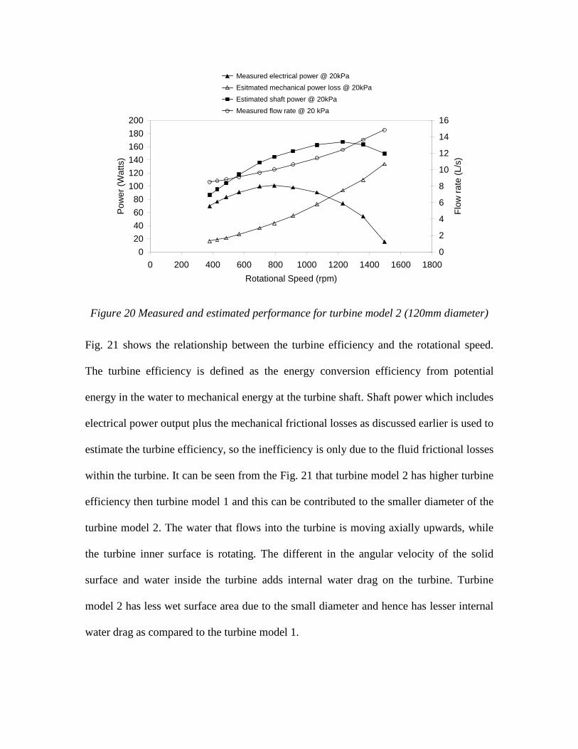
Fig. 19 and Fig. 20 shows the relationship between the measured/estimated power and the

rotational speed, at the same time the flow rate is shown on the secondary y-axis. The

measured values show actual measurements, e.g. measured electrical power is equal to

the product of measured voltage and current output from the generator. Whereas the

estimated values show the sum of measured power and power lost in friction. The

estimated mechanical power loss represents the sum of power loss from the inlet lip seal,

bearings and air drag. To estimate the sum of mechanical power loss the installed turbine

is rotated using a DC motor at different rotational speeds. Here the power consumed by

the DC motor at different rotational speeds represents the overall mechanical losses

associated with the turbine and DC generator (motor) assembly. Overall it can be seen

that for both the turbines the frictional power loss increases as the rotational speed

increases. A closer look at the graphs shows that the mechanical power losses in turbine

model 2 are less as compared to the mechanical power losses in turbine model 1 at a low

rotational speed. For example, for turbine model 1 at 600rpm the mechanical power loss

is about 58Watts, whereas for turbine model 2 at 600rpm the mechanical power loss is

about 30Watts. This reduced mechanical power loss is a result of reduced air drag losses

due to small rotor diameter of turbine model 2. From experiments it was observed that the

air drag increases as the turbine exit nozzle width is increased, this was due to the shape

of turbine drifting away from a perfect circle to more elliptical as the exit nozzle width is

increased.

Figure 18 Picture of two split reaction water turbines

020406080

100120140160180200

0 100 200 300 400 500 600 700 800 900Rotational Speed (rpm)

Pow

er (W

atts

)

0

2

4

6

8

10

12

14

16

18

Flow

rate

(L/s

)

Measured electrical power @ 20kPa

Esitmated mechanical power loss @ 20kPa

Estimated shaft power @ 20kPa

Measured flow rate @ 20kPa

Figure 19 Measured and estimated performance for turbine model 1 (240mm diameter)

Turbine Model 2 Turbine Model 1

020406080

100120140160180200

0 200 400 600 800 1000 1200 1400 1600 1800Rotational Speed (rpm)

Pow

er (W

atts

)

0

2

4

6

8

10

12

14

16

Flow

rate

(L/s

)

Measured electrical power @ 20kPa Esitmated mechanical power loss @ 20kPa Estimated shaft power @ 20kPa Measured flow rate @ 20 kPa

Figure 20 Measured and estimated performance for turbine model 2 (120mm diameter)

Fig. 21 shows the relationship between the turbine efficiency and the rotational speed.

The turbine efficiency is defined as the energy conversion efficiency from potential

energy in the water to mechanical energy at the turbine shaft. Shaft power which includes

electrical power output plus the mechanical frictional losses as discussed earlier is used to

estimate the turbine efficiency, so the inefficiency is only due to the fluid frictional losses

within the turbine. It can be seen from the Fig. 21 that turbine model 2 has higher turbine

efficiency then turbine model 1 and this can be contributed to the smaller diameter of the

turbine model 2. The water that flows into the turbine is moving axially upwards, while

the turbine inner surface is rotating. The different in the angular velocity of the solid

surface and water inside the turbine adds internal water drag on the turbine. Turbine

model 2 has less wet surface area due to the small diameter and hence has lesser internal

water drag as compared to the turbine model 1.

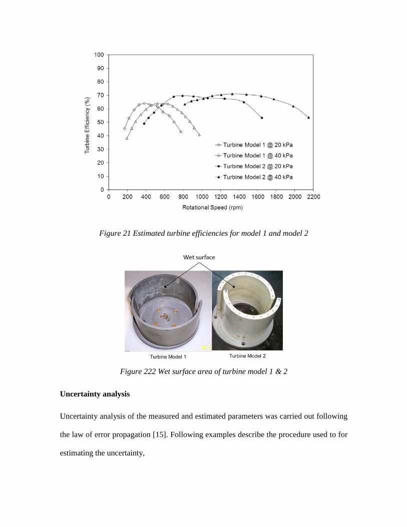
Figure 21 Estimated turbine efficiencies for model 1 and model 2

Figure 222 Wet surface area of turbine model 1 & 2

Uncertainty analysis

Uncertainty analysis of the measured and estimated parameters was carried out following

the law of error propagation [15]. Following examples describe the procedure used to for

estimating the uncertainty,

The volume flow rate of the water flowing through the turbine was estimated by using the

measurements from the volume flow meter that read total volume flow and the reading

from the stop watch. Here the estimate volume flow rate ( )V is equal to the measured

water volume ( )V divided by the measured time ( )t .

tVV =

•

(38)

Following two equation have been derived by taking partial derivative of volume flow

rate with respect to measured volume and with respect to measure time,

VtV

V∂=

∂∂•

1

(39)

ttV

tV

∂−=∂∂

•

2 (40)

The following equation used to estimate the absolute uncertainty in the estimation of

volume flow rate ( )V∆ has been derived using the above two partial derivatives and the

law of error propagation,

2

2

21

∆−+

∆=∆

•

ttVV

tV

(41)

The relative uncertainty in the estimation of volume flow rate is the ratio of the absolute

uncertainty and the estimated volume flow rate as shown in the following equation.

••

•

∆−+

∆

=∆

V

ttVV

t

V

V

2

2

21

(42)

Here, ( )V∆ is the absolute uncertainty of the volume flow meter as specified by the flow

meter manufacturer, ( )t∆ is the absolute uncertainty of the stop watch as specified by the

stop watch manufacturer including the human reflex uncertainty. The human reflex

uncertainty becomes negligible for time measurements of above 30sec.

The relative velocity AVVr

= of water jets at both the exit nozzles is equal to the

estimated volume flow rate ( )V divided by the total exit nozzle area ( )A . So the absolute

uncertainty in the estimation of the velocity can be calculated using the following

equation derived using the law of error propagation,

2

2

21

∆−+

∆=∆ A

AVV

AVr

(43)

rr

r

V

AAVV

A

VV

2

2

21

∆−+

∆

=∆

••

(44)

The absolute uncertainty in estimating the value of k-factor can be calculated from the

following equation. This equation has been derived from the law of propagation and by

using the value of estimated relative velocity, measured rotational speed, measured head

and equation (37).

( ) ( )

∆×+

−+

∆+

∆+

∆×=∆ r

rrrr

VRgHVV

RV

RRV

Hgk 2222

2

2

22

2

22

2 21222 ωωωω (45)

Following the similar procedure as discussed above uncertainty analysis of the

experimental performance results has been conducted. The uncertainty analysis of the

experimental data from stationary test shows that the estimated torque has a relative

uncertainty of ±4.41% and the measured torque has a relative uncertainty of ±1.13%. The

relative uncertainty in the measured volume flow rate is about ±2.5% and the relative

uncertainty in the estimated k-factor is only ±2.53%. The relative uncertainty in the

estimation of the shaft power is estimated as maximum ±5.02%. The relative uncertainty

in the estimation of the rate of potential energy supplied to the turbine is estimated as

±2.70%. From these calculated quantities of the relative uncertainties it is confirmed that

the instrumentation and experimental procedures used for conducting the performance

tests on the simple reaction turbine models have very high level of confidence and

reliability.

Conclusion

The performance of an idealized reaction turbine has been represented in dimensionless

equations and curves. For the ideal situation of a flow system and turbine without fluid

friction losses, it is shown that the self pumping action implicit in energy conservation

modifies the traditional expectations for this class of reactive turbine. In particular, the

speed, power and mass flow rate will tend to infinities as the torque approaches half of

the stalled value. From the theoretical analysis it is seen that mass flow rate increases

with the increase in the rotational speed due to the centrifugal pumping action. The

variation of m with rotational speed is almost linear and the effect of supply head on the

mass flow rate vanishes at high rotational speeds. The self-pumping effect, i.e. increase in

mass flow rate with rotational speed is true for the practical case with frictional losses

and experimental results have validated this phenomenon.

The ideal characteristics modeled suggest that the simple reaction turbine may have

application to high speed power generation from low head water supplies. As shown by

the non-dimensional analysis a simple reaction water turbine has higher efficiency at high

speeds. Although it is seen that for a practical situation with fluid frictional losses the

simple reaction turbine will never experience the runaway condition of infinite speed.

Further the maximum power and efficiency of a turbine with frictional losses will

dependent on the k-factor and this has been concluded from the experimental results.

The test results have shown that turbine model 2 has higher turbine efficiency as

compared with turbine model 1 for the same supply head, but at higher rotational speeds.

This behavior of the turbine model 2 can be attributed to the fact that the model 2 has

smaller diameter and hence the wet surface area is less. This helps to reduce the energy

loss from the internal water drag that is prominent in the turbine model 1 due to larger

diameter and hence larger wet surface area.

The uncertainty analysis has shown that the experimentally measured results and the

estimated results have reasonable relative uncertainties and so the findings of this study

can be used as a basis for future investigation. This analysis shows that a simple reaction

turbine can convert low head hydro power to mechanical power with high efficiency. It is

also very simple to fabricate the simple reaction turbines that have been experimentally

investigated.

References

1. Wilson, P.N., Water Turbines. A Science Museum Booklet. 1974: Her Majesty's

Stationery Office.

2. Balje, O.E., "Turbo-machines, a guide to design, selection and theory". 1981:

John Wiley & Sons.

3. Bartle, A., Hydropower potential and development activities. Energy Policy,

2002. 30(14): p. 1231-1239.

4. Shepherd, D.G., Principles of turbomachinery. 1956: Macmillan.

5. Leo, B.S. and S.T. Hsu, A simple reaction turbine as a solar engine. Solar

Energy, 1960. 4(2): p. 16-20.

6. J.F., B., "The Rotating Nozzle (Hero's) Turbine". ASME, 1960(60-WA-293).

7. Daugherty, R.L., Franzini, Joseph B. Finnemore, E. John., Fluid mechanics with

engineering applications. 1989: McGraw-Hill.

8. Balje, O.E., Turbomachines: A guide to design, selection and theory. 1981, NY:

John Wiley.

9. Duncan W.J., T.A.S., and Young A.D., Mechanics of Fluids. 1970: Edward

Arnold.

10. Davis, J.R.A., Science in Modem Life : Engineering. 1st ed. Science in Modem

Life, ed. F. J.W. Vol. 6. 1910, London UK: The Gresham Publishing Company.

11. Daugherty R.L., I.A.G., Fluid Mechanics with Engineering Applications. 1954:

McGraw-Hill Book Company.

12. R.K., T., Principles of Turbomachinery. 1984: E. & F.N. Spon.

13. Date, A., Low head simple reaction water turbine, in School of Aerospace

Mechanical and Manufacturing Engineering2009, RMIT University: Melbourne.

p. 251.

14. Date, A. and A. Akbarzadeh, Design and analysis of a split reaction water

turbine. Renewable Energy, 2010. 35(9): p. 1947-1955.

15. Drosg, M., Dealing with Uncertainties A Guide to Error Analysis. 2007, Berlin:

Springer-Verlag