ABSTRACT
An SEGF Study Of The Rh(001) Surface
Mark R. Mastin, M.S.
Advisor: Gregory A. Benesh, Ph.D.
A self-consistent study of Rh(001) has been performed using the surface
embedded Green function method. Calculations have been performed by
embedding a three-layer slab onto a bulk rhodium substrate. The calculated
work function and surface core level shifts are in good agreement with other
theoretical work. Additionally, bulk band structures have been calculated, and
the projected bulk band structure has been constructed. Densities of states have
also been calculated in order to identify surface states and surface resonances. In
addition to a contour plot of the total charge density, charge densities have been
plotted for several of the surface states.

Page bearing signatures is kept on file in the Graduate School.
An SEGF Study of the Rh(001) Surface
by
Mark R. Mastin, B.S.
A Thesis
Approved by the Department of Physics
___________________________________
Gregory A. Benesh, Ph.D., Chairperson
Submitted to the Graduate Faculty of
Baylor University in Partial Fulfillment of the
Requirements for the Degree
of
Master of Science
Approved by the Thesis Committee
___________________________________
Gregory A. Benesh, Ph.D., Chairperson
___________________________________
Kenneth T. Park, Ph.D.
___________________________________
Joe C. Yelderman, Jr., Ph.D.
Accepted by the Graduate School
August 2007
___________________________________
J. Larry Lyon, Ph.D., Dean

Copyright © 2007 by Mark R. Mastin
All rights reserved

iii
TABLE OF CONTENTS List of Figures ..................................................................................................... v
List of Tables ....................................................................................................... vii
Acknowledgments.............................................................................................. viii
Dedication ........................................................................................................... ix
Chapter
I. Introduction................................................................................................... 1
II. Surface Electronic Structure Calculations ........................................................ 4
A. The Surface Problem.................................................................................. 4
B. Surface Embedded Green Function Method ............................................... 8
C. Embedding Potential.................................................................................. 13
D. Basis Functions.......................................................................................... 15
1. Interstitial Region................................................................................. 16
2. Muffin-Tin Spheres.............................................................................. 16
3. Vacuum Region ................................................................................... 17
E. Self-Consistency ........................................................................................ 17
F. Mixing....................................................................................................... 18
III. Computational Details ..................................................................................... 21
A. Embedding Potential.................................................................................. 21
B. Self-Consistent Charge Density.................................................................. 24
C. Bulk Band Structure and Projected Bulk Band Structure ............................ 24
D. Density of States........................................................................................ 26

iv
IV. Results and Analysis of Clean Rhodium .......................................................... 27
A. Work Function........................................................................................... 27
B. Surface Core-Level Shifts .......................................................................... 30
C. Projected Bulk Band Structure ................................................................... 34
D. Densities of States...................................................................................... 42
E. Charge Density .......................................................................................... 46
V. Conclusion ...................................................................................................... 60
References ........................................................................................................... 62
v
LIST OF FIGURES
Figure 2.1 Depiction of the Surface Region I (including vacuum) and Substrate
(bulk) Region II utilized in the SEGF method. ..................................... 9 2.2 Surface and bulk are separated by the complicated surface S, but the effective embedding interface S0 is used............................................... 14 2.3 Sketch depicting the three distinct sub-regions of the Surface Region. 15 3.1 Top view of two layers of rhodium....................................................... 22 3.2 Top view of Rh(001) demonstrating basis vectors. .............................. 23 3.3 Atoms in the surface region. .................................................................. 23 3.4 k points used to determine the projected bulk band structure........... 25 4.1 Bulk band structure at ! [(0,0)] plotted as a function of k
!. ................. 35
4.2 Bulk band structure at (0.125, 0) plotted as a function ofk
!. .................. 36
4.3 Bulk band structure at X [(0.5,0)] plotted as a function ofk
!. ............... 36
4.4 Bulk band structure at M [(0.5,0.5)] plotted as a function ofk
!. ........... 37
4.5 PBBS of even symmetry for the ! X line in the SBZ. ......................... 38 4.6 PBBS of odd symmetry for the ! X line in the SBZ. ........................... 39 4.7 PBBS for the ! X line in the SBZ. ......................................................... 40 4.8 PBBS for the entire SBZ. ........................................................................ 41 4.9 DOS at !. ................................................................................................ 43 4.10 DOS at X. ................................................................................................ 43 4.11 DOS at M. ............................................................................................... 44

vi
4.12 PBBS with DOS points overlayed.......................................................... 45 4.13 Total charge density on Rh(001) surface sampled on ten special
k points. ................................................................................................... 47 4.14 Total charge density on Rh(001) surface sampled on ten special
k points. ................................................................................................... 48 4.15 Valence charge density of the surface resonance of ! (0, 0) at
EF – 5.14 eV. ............................................................................................. 49 4.16 Valence charge density of the (0.25, 0) surface state at EF – 4.80 eV. .. 50 4.17 Valence charge density of the (0.5, 0) surface state at EF – 4.12 eV. .... 51 4.18 Valence charge density of the (0.5, 0.125) surface state at EF – 2.56 eV. 52 4.19 Valence charge density of the (0.5, 0.25) surface state at EF – 0.20 eV 53 4.20 Valence charge density of the (0.5, 0.3125) surface state at EF – 3.98 eV. 54 4.21 Valence charge density of the (0.5, 0.5) surface state at EF + 0.98 eV. . 55 4.22 Valence charge density of the (0.3125, 0.3125) surface state at
EF – 0.58 eV............................................................................................... 56 4.23 Valence charge density of the (0.1875, 0.1875) surface state at
EF – 3.92 eV............................................................................................... 57 4.24 Valence charge density of the (0.0625, 0.0625) surface state at
EF – 3.03 eV............................................................................................... 58

vii
LIST OF TABLES
Table
4.1 Comparison of experimental and theoretical work functions. ..................... 28
4.2 Surface and Sub-surface Core Level Shifts. .......................................... 33

viii
ACKNOWLEDGMENTS
I am forever grateful to Dr. Greg Benesh for his seemingly infinite
patience through this long process. He never gave up on me and his
encouragement and persistence helped to carry me through. His wisdom and
guidance were invaluable and he was consistently generous with both. Thank
you, also, to Dr. Kenneth Park and Dr. Joe Yelderman for their willingness to
serve on my committee on short notice.
I would also like to thank the Graduate School and the Department of
Physics for allowing me the opportunity to study and for giving me “one last
chance.”
I must thank my colleagues in Information Technology Services that
helped me throughout the process: they encouraged me; they provided
necessary technical assistance; and they allowed me the time required to
complete my study.
Last, but certainly not least, thank you to my family for encouraging me
throughout this process. Thanks for always being there for me (even when I
could not return the favor). I hope now to give you back some of the time that
you have lent me.

ix
To
Regina, the love of my life. You never gave up on me!
Drew, Evan, and Lindsay. Don’t quit and never say never.
Mom and Dad. Thanks for teaching me to keep reaching.
Granddaddy. I’m sorry you didn’t see me finish, but you helped me get there.

1
CHAPTER ONE
Introduction
Solid surfaces come in two types: amorphous (in which there is no regular
array of atoms) and crystalline (in which a regular pattern of atoms is repeated
continually). However, all solids do form crystals under certain circumstances,
which results in a computational simplification. For this reason, crystal surfaces
are more commonly studied. A theoretical study that models a physical crystal
would require a solution to an N-body problem, with N on the order of 1023.
Periodic boundary conditions and crystalline symmetry only reduce the problem
so far: N remains on the order of 109. Unfortunately, this problem is
unmanageable, even with today’s supercomputers. Certain assumptions and
approximations must be made to reduce the size of the problem in order to solve
accurately and within a reasonable time period.
Previously, the most common theoretical approach to the surface problem
has been to model the crystal as a slab, typically five to nine atomic layers thick,
and extending to infinity in the x-y plane. This method allows determination of
several aggregate surface electronic properties such as work functions, charge
densities, and spin densities. While this approximation reduces the problem to a
manageable size, it also contains limitations. A thicker slab would presumably
give more accurate results, but the amount of computational resources required
becomes too great. Another limitation of these slab-based methods is the
inability of the valence electrons to properly screen two surfaces that are in close
proximity to each other. As a result, states arising from the two surfaces interact

2
unphysically with each other, creating pairs of hybridized states at different
energies.
Benesh and Inglesfield1,2,3 have developed a technique which more
accurately describes the surface using a semi-infinite geometry. The Surface
Embedded Green Function (SEGF) method treats the surface as a semi-infinite
crystal using an embedding potential to exactly represent the influence on the
surface of an infinite bulk substrate. The SEGF method has been used to obtain
excellent results for Al(001)4, Al(111)5, Al(110)6, Fe(001)7, Pt(001)8, as well as
chemisorbed surfaces such as O/Pt(001)9, CO/Fe(001)10, and N/Fe(001)11. The
general nature of the surface problem and the specifics of the SEGF method will
be described in chapter two.
In chapter three, the computational details of the SEGF method as applied
to the surface of the 4d transition metal rhodium are discussed. Rhodium has an
important industrial application in its use as an exhaust catalyst for nitric oxide
reduction and carbon monoxide oxidation.12 The present characterization of the
clean Rh(001) surface is necessary for a later determination of the interactions
between rhodium and various overlayers, such as NO and CO, atop the surface.
The intent is to gain a fundamental understanding of such reactions in an effort
to achieve greater efficiency and increased gas reduction. As noted, the SEGF
method has been used very successfully for many metals, both clean and with
overlayers; however, this study of rhodium represents the first application of the
SEGF method to a 4d transition metal surface.
The fourth chapter discusses the results of the SEGF study of clean
rhodium. The work function is calculated and compared to other theoretical and
experimental results. The accuracy of the work function is commonly viewed as

3
a measure of the accuracy of the method. The surface core level shift (SCLS) is
also evaluated and compared with other results. The band structure of Rh(001)
has been investigated to determine the positioning of surface states and surface
resonances. These are compared to other theoretical models and to available
experimental results.
4
CHAPTER TWO
Surface Electronic Structure Calculations
A. The Surface Problem
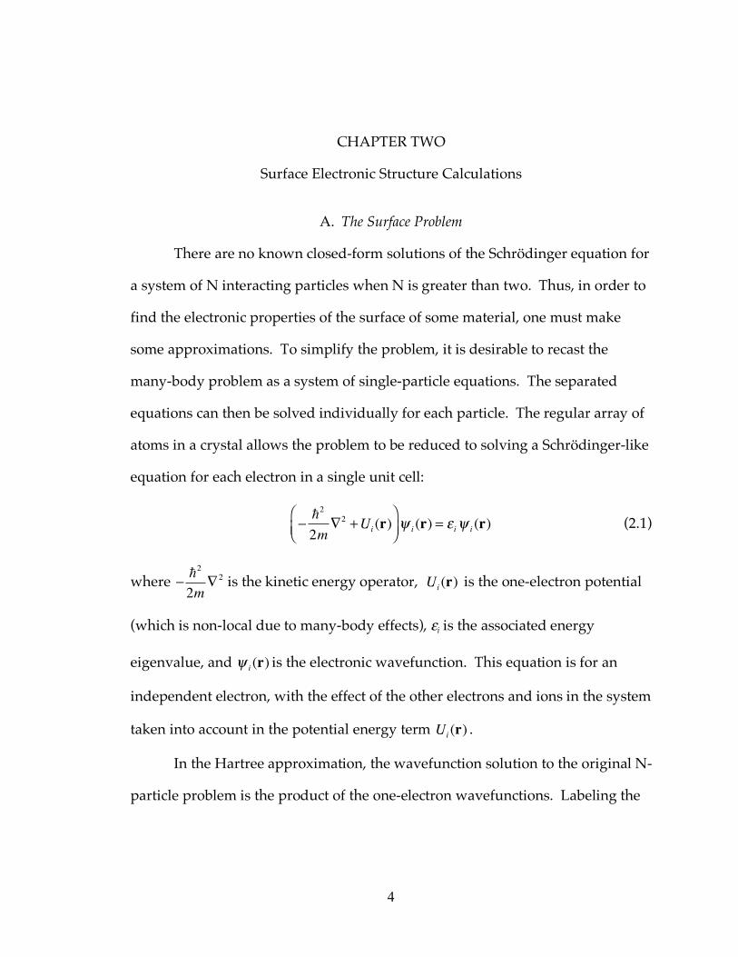
There are no known closed-form solutions of the Schrödinger equation for
a system of N interacting particles when N is greater than two. Thus, in order to
find the electronic properties of the surface of some material, one must make
some approximations. To simplify the problem, it is desirable to recast the
many-body problem as a system of single-particle equations. The separated
equations can then be solved individually for each particle. The regular array of
atoms in a crystal allows the problem to be reduced to solving a Schrödinger-like
equation for each electron in a single unit cell:
!!2
2m"2
+Ui(r)
#$%
&'()
i(r) = *
i)
i(r) (2.1)
where
�
!!2
2m"2 is the kinetic energy operator, U
i(r) is the one-electron potential
(which is non-local due to many-body effects), εi is the associated energy
eigenvalue, and !i(r) is the electronic wavefunction. This equation is for an
independent electron, with the effect of the other electrons and ions in the system
taken into account in the potential energy term Ui(r) .
In the Hartree approximation, the wavefunction solution to the original N-
particle problem is the product of the one-electron wavefunctions. Labeling the

5
N-particle wavefunction as Ψ, the N-electron Schrödinger equation for the
crystal system is
H! = "!2
2m i
2# ! " Ze21
ri " R!
R
$%
&'(
)*+1
2
e2
ri " rj! = E!
i+ j$
i=1
N
$ . (2.2)
The second term, the negative potential energy term, represents the electrostatic
potential at ri due to the fixed nuclei at the points R of the Bravais lattice. The
positive potential energy term is the electron-electron repulsion; it is this
interaction term that makes equation (2.2) intractable. Some simplification must,
therefore, be made to approximate this electron-electron interaction.
Returning to the one-particle equation (2.1), an initial approximation is
made for Ui(r) . U
i(r) should contain the potential of the ions:
Uion(r) = !Ze
2 1
r ! RR
" (2.3)
But Ui(r) also needs to contain, at least approximately, the influence of each of
the remaining electrons. If these other electrons are treated as a distribution of
negative charge, then the potential energy due to electrostatic repulsion is
Uel(r) = !e dr '"(r ')
1
r ! r '# , (2.4)
where
!(r) = "e #i(r)
2
i
$ (2.5)
is the charge density and the sum is over all occupied one-electron levels. The
iterative process begins with an initial guess of !(r) . (!(r) is often approximated
from calculated atomic charge densities.) With the starting charge density, Uel is

6
then calculated and added to Uion to give the initial approximation of Ui(r) . The
Schrödinger equation is solved, and the output charge density constructed from
the one-electron wavefunctions. This process is repeated until the output charge
density of two successive iterations does not change significantly. This point is
known as self-consistency.
Although the Hartree approximation has been successful in obtaining
many properties of atomic system (at least qualitatively), it has its shortcomings
as well. First, it fails to account for the anti-symmetry of the electron
wavefunctions. Second, it does not adequately incorporate correlation effects
between pairs of electrons, since electrons interact directly with one another−not
just through the averaged density.
If Hartree’s product wavefunction is replaced by a Slater determinant of
one-electron wavefunctions in the form:
!(r1s1,r2s2,…,r
NsN) =
"1(r1s1) "
1(r2s2) … "
1(r
NsN)
"2(r1s1) "
2(r2s2) … "
2(r
NsN)
! ! " !
"N(r1s1) "
N(r2s2) … "
N(r
NsN)
, (2.6)
the proper anti-symmetrization of the total wavefunction is obtained. Inserting
(2.6) into the variational expression for the energy,
H!=
! H !
! !, (2.7)
then minimizing with respect to the !i's produces the Hartree-Fock equations,
!!2
2m
2
"# i (r) +Uion(r)# i (r) +U
el(r)# i (r) !
! d $re2
r ! $r# j
%( $r )# i ( $r )# j (r)& si s j'
j
( = )i# i (r)
(2.8)
7
with Uion and Uel defined previously. The last term on the left hand side is
called the exchange term and distinguishes the Hartree-Fock equations from that
of Hartree. (An additional slight variation is that the Uel(r) in Hartree does not
contain the contribution of the ith electron, while Hartree-Fock does.) Although
the Hartree-Fock equations are an improvement over the Hartree equations, they
are still not simply solvable.13
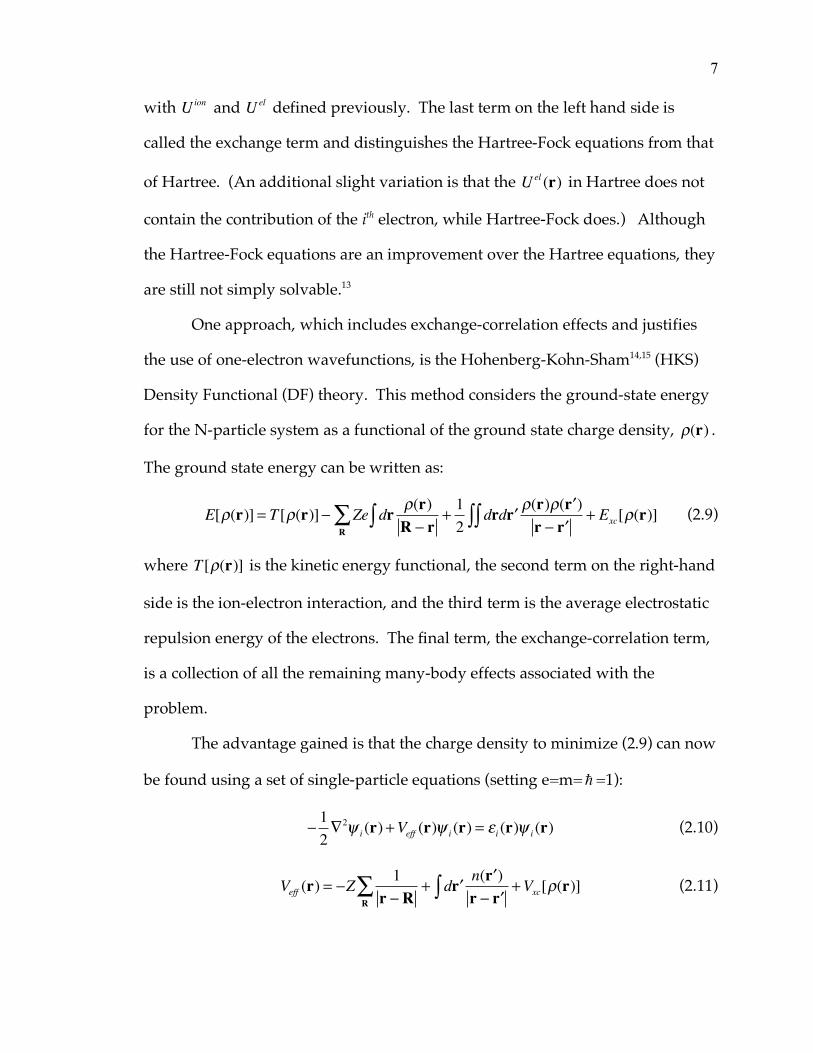
One approach, which includes exchange-correlation effects and justifies
the use of one-electron wavefunctions, is the Hohenberg-Kohn-Sham14,15 (HKS)
Density Functional (DF) theory. This method considers the ground-state energy
for the N-particle system as a functional of the ground state charge density, !(r) .
The ground state energy can be written as:
E[!(r)] = T [!(r)]" Ze dr!(r)R " r#
R
$ +1
2drd %r
!(r)!( %r )r " %r## + E
xc[!(r)] (2.9)
where T [!(r)] is the kinetic energy functional, the second term on the right-hand
side is the ion-electron interaction, and the third term is the average electrostatic
repulsion energy of the electrons. The final term, the exchange-correlation term,
is a collection of all the remaining many-body effects associated with the
problem.
The advantage gained is that the charge density to minimize (2.9) can now
be found using a set of single-particle equations (setting e=m= ! =1):
!1
2"2# i (r) +Veff (r)# i (r) = $i (r)# i (r) (2.10)
Veff (r) = !Z1
r ! RR
" + d #rn( #r )r ! #r$ +Vxc[%(r)] (2.11)

8
where n(r) = !i
2" , summed over the occupied orbitals, and Vxc[!(r)] contains
the exchange and correlation interactions.
A common approximation to Vxc[!(r)] is made in the Local Density
Approximation (LDA). When applying the LDA, the exchange-correlation
energy density of each infinitesimal volume of the inhomogeneous electron
distribution is assumed to be equivalent to the exchange-correlation energy
density of a homogeneous electron gas with the same density, i.e.
Vxc(r) = V
xc!(r)[ ] . It is worthwhile to point out that the only approximation made
in the DF method is the calculation of many-body effects which are included in
the Vxc
term.16
B. Surface Embedded Green Function Method
As mentioned earlier, the most common geometry used in surface
calculations is the slab, in which a crystal is modeled using five to nine layers of
atoms. Slab-based methods are successful in calculating aggregate properties,
but are not as successful in calculating properties which require individual
wavefunctions on the surface or in the bulk. Benesh and Inglesfield have pointed
out certain problems associated with slab-based methods.3 For instance, the bulk
is not properly represented by the few (three to seven) layers which separate the
two surfaces. There is also an unphysical interaction between the two surface
layers, often splitting surface states arising from the two surfaces into hybridized
pairs.
Desiring to improve upon these methods for surface calculations, Benesh
and Inglesfield1,2,3 developed the SEGF method. In this method, an embedding

9
potential for a semi-infinite substrate (Region II in Figure 2.1) is obtained from
the substrate Green function. The vacuum along with a few surface layers
(Region I) are then embedded onto this substrate, as shown in Figure 2.1. The
inclusion of the embedding potential in the Schrödinger equation for Region I
causes surface wavefunctions to match onto bulk solutions across the embedding
surface.
Figure 2.1. Depiction of the Surface Region I (including vacuum) and Substrate (bulk) Region II utilized in the SEGF method.

10
To obtain the solutions in Region I, an expression is first derived for the
expectation value of the energy of a trial function !(r) , defined as a trial
wavefunction !(r) in Region I, and in Region II as ! (r) . ! (r) is the exact
solution of the Schrödinger equation at some energy ε in the bulk. An additional
requirement is that !(r)and ! (r) must match amplitudes across the interface S.
In atomic units e=m= ! =1:
H! (r) = ("1
2
2# +V
bulk(r))! (r) = $! (r) , with r in Region II. (2.12)
The energy expectation value for ! is given by:
E =! H !
! !=
" H "I+ # $ $
II+ ! H !
S
" "I+ $ $
II
(2.13)
where the first term in the numerator is the expectation value in the surface-
vacuum region, the second term is the expectation in the bulk, and the third term
is:
! H !S=1
2d2rs" *(r
s)#"(r
s)
#ns
$#% (r
s)
#ns
&
'()
*+s, (2.14)
This term accounts for a discontinuity in derivative between ϕ and ψ across the
substrate-surface interface, leading to the integral over the embedding surface S.
Therefore, the total expectation energy in integral form is:
E =
d3r! *
(r)H!(r)I" + # d
3(r)$ *
(r)$ (r)II" +
1
2d2rs! *(r
s)%!(r
s)
%ns
&%$ (r
s)
%ns
'()
*+,s
"d3r! *
(r)!(r)I" + d
3(r)$ *
(r)$ (r)II"
.
(2.15)
The Green function G0 for Region II satisfies the differential equation

11
(!1
2r
2" +V
bulk(r) ! #)G
0(r, $r ) = % (r ! $r ) , r, !r in II. (2.16)
G0 is chosen to satisfy the boundary condition that its normal derivative
vanishes at the interface r = rS
,
!G0(r
s, "r )
!ns
= 0 . (2.17)
Using Green’s theorem, a relation can be obtained between the amplitude of the
wavefunction in II and its normal derivative at the interface:
! (r) = "1
2d2rSG0(r,r
S)#! (r
S)
#nS
S$ . (2.18)
With r on the interface, this becomes:
! (rS) = "
1
2d2 #r
SG0(r
S, #r
S)$! ( #r
S)
$ #nS
S% . (2.19)
The inverse of (2.19) gives the desired result, ! "#
"nS
in terms of ! (rS) , which at
the interface is equal to!(rS) :
!" (rS)
!nS
= #2 d2 $r
SG0
#1(r
S, $r
S)%( $r
S)
S& (2.20)
An expression is still needed to replace the volume integral over Region II.
Inglesfield1 has shown that:
d3r! *
(r)! (r)II" = # d
3rS
S" d
3 $rS% *(r)
&G0
#1(r
s, $r
S)
&'%( $r
S)
S" (2.21)
E can now be expressed purely in terms of the Region I trial function
!(r) and the bulk Green function G0, such that (2.15) becomes:

12
E =
d3r! *
(r)H!(r)I" +
1
2d2rS! *(r)
#!(rS)
#nS
S" +
$
%&
d2rS
S" d
2 'rS! *(r)G
0
(1(r
s, 'r
S)!( 'r
S)
S" ( ) d
2rS
S" d
2 'rS! *(r)
#G0
(1(r
s, 'r
S)
#)!( 'r
S)
S"
*
+,
d3r! *
(r)!(r)I" ( d
2rS
S" d
2 'rS! *(r)
#G0
(1(r
s, 'r
S)
#)!( 'r
S)
S"
.
(2.22)
The trial function, !(r) , is expanded in terms of a set of basis functions, !i(r) ,
[!(r) = ai"i(r)
i
# ] and E is then minimized with respect to small changes in
!(r) , resulting in:
(Hij + (G0
!1)ij + (E ! ")
#(G0
!1)ij
#E)
j
$ aj = E Oijajj
$ (2.23)
where
Hij = d3r !k
*(r)H!i (r)
I" +1
2d2rS !k
*(rS )
#!i (rS )
#nSS" , (2.24)
(G0
!1)ij = d
2rS
S
" d2rS#G
0
!1(rS ,rS
#;E)$i (rS# )
S
" , (2.25)
and Oij = d
3r !i
*(r)! j (r)" . (2.26)
Equation (2.23) now shows G0
!1 as a potential added to the surface
Hamiltonian. As such, G0
!1 contains all the information about the substrate
needed for the surface calculation and is the embedding potential.
The surface Green function may be calculated instead of the individual
wavefunctions. We have chosen to expand G(r, !r ;E) in terms of a set of basis
functions as:

13
G(r, !r ;E) = gij (E)"i (r)" j ( !r )ij
# . (2.27)
A matrix equation comparable to (2.23) is then computed, and, evaluating E at ! ,
the following is obtained:
(Hij + (G0
!1)ij !
j
" EOij )gij (E) = # ij (2.28)
from which the gij ’s are computed. At this point, with the surface Green
function having been obtained, other interesting properties of the surface may be
calculated.
C. Embedding Potential
As shown in (2.23) and (2.28), the embedding potential
�
G0
!1 is included as
an extra (embedding) potential in the surface region Hamiltonian. Since
�
G0
!1 is
related to the reflection properties of a crystal, one technique for obtaining the
embedding potential is the layer-doubling method, commonly used in low
energy electron diffraction (LEED) analyses.18 In terms of the reflection matrix R,
the Fourier components of
�
G0
!1 are obtained from the expression:
G0,K
!1=
1
2" (1! R)(1+ R)!1 (2.29)
where K is the wave vector, R is the reflection matrix, and
! = K "m
2 # ! "m
2= K
m
2+ k
z
2 (2.30)
with Km=K + Gm, where Gm is a reciprocal lattice vector.
In figure 2.2, it is clear that the interface S may not be a simple surface
over which to evaluate the matrix-element integrals. Benesh and Inglesfield2,3
overcame this difficulty by transferring
�
G0
!1 from the surface S to S0, a more

14
convenient flat surface with a constant potential between S and S0. This
procedure is further justified by Crampin et al.17
Figure 2.2. Surface and bulk are separated by the complicated surface S, but the effective embedding interface S0 is used. (from Ref. 3, p. 6684)

15
D. Basis Functions
The surface region I is further divided into three sub-regions (shown in
Figure 2.3): muffin-tin (MT) spheres centered around the nuclei, the interstitial
region between the muffin-tin spheres, and the vacuum region. Each of these
sub-regions contains a different characteristic potential. Within the muffin-tin
Figure 2.3. Sketch depicting the three distinct sub-regions of the Surface Region. (Adapted from Ref. 10, p. 18)

16
spheres, the potential is largely spherical due to the atomic cores. In the
interstitial region, the potential is relatively flat; while in the vacuum, the
potential has a strong z -dependence, but relatively weak x- and y-dependence.
Due to the varying nature of the potential, solutions to the surface problem have
a different characteristic form in each of the three sub-regions. For this reason,
Benesh and Inglesfield use Linear Augmented Plane Waves (LAPWs) as the basis
functions for the SEGF method.
1. Interstitial Region
Since the potential is relatively flat, plane waves of the following form are
used:
!m,n
+(r)
!m,n
"(r)
#$%
&%=
2
'eiKm •R (
cos(knz), n even
sin(knz), n odd
)*+
(2.31)
kn=n!
D and ! = AD where D is the slab thickness, A is the surface area of the
unit cell, and D defines a plane slightly larger than D (see Figure 2.3), which
aids in the matching of the wavefunctions at the vacuum and bulk boundaries.
Note that n is even for the symmetric (+) case and odd for the antisymmetric (-)
case, as determined by reflection z! "z .
2. Muffin-Tin Spheres
Since the potential is highly spherical within the muffin-tin spheres, the
LAPW for this region is composed of radial u! and energy derivative
!u"
solutions of the scalar-relativistic Schrödinger equation:
17
!m,n
+(r)
!m,n
"(r)
#$%
&%=
AL ,'+(K)
AL ,'"(K)
()%
*%
#$%
&%+ u
!,' +
BL ,'+(K)
BL ,'"(K)
()%
*%
#$%
&%+ "u
!,'
,
-..
/
011YL(2) +
i!
i!"1
()%
*%L
3 (2.32)
Benesh and Inglesfield have found that ! -values up to !max
= 8 usually suffice to
reach convergence. A and B coefficients are determined by matching χ and its
radial derivative across the surface of the MT spheres, denoted by α.
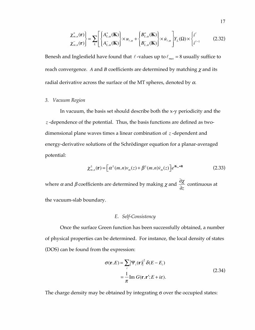
3. Vacuum Region
In vacuum, the basis set should describe both the x-y periodicity and the
z -dependence of the potential. Thus, the basis functions are defined as two-
dimensional plane waves times a linear combination of z -dependent and
energy-derivative solutions of the Schrödinger equation for a planar-averaged
potential:
!m,n
±(r) = " ±
(m,n)vm(z) + # ±
(m,n) !vm(z)$% &'e
iKm •R (2.33)
where α and β coefficients are determined by making χ and !"!z
continuous at
the vacuum-slab boundary.
E. Self-Consistency
Once the surface Green function has been successfully obtained, a number
of physical properties can be determined. For instance, the local density of states
(DOS) can be found from the expression:
! (r,E) = "
i(r)
2# (E $ E
i)
i
%
=1
&Im G(r, 'r ;E + i().
(2.34)
The charge density may be obtained by integrating σ over the occupied states:

18
n(r) =1
!Im dE G(r, "r ;E)
#$
EF
% (2.35)
The integration is performed using a semi-circular contour in the upper half
complex plane.
Once the charge density is known, it may be used to solve Poisson’s
equation for the electrostatic potential
!2Ves(r) = "4#$(r) (2.36)
using a pseudo-charge method developed my Weinert.19 In Weinert’s method,
the MT charge density is (temporarily) replaced by a pseudo-charge density
which has the same multipole moments as the actual charge density in the MT
spheres. The pseudo-charge is then Fourier expanded and used to solve
Poisson’s equation. The resulting solution is correct throughout the interstitial
and vacuum sub-regions and on the MT boundaries. The MT boundary
conditions allow Poisson’s equation to be solved in the MT spheres using the
actual MT charge density. The exchange-correlation potential is then added to
the electrostatic potential to create the new surface potential. This process is
repeated until self-consistency is reached.
F. Mixing
As mentioned previously, the SEGF method is an iterative method.
Obviously, it is desirable to achieve convergence in a reasonable number of
cycles. One approach is to take the results from one iteration and insert it as the
input for the next iteration of the SEGF program. However, this approach is
unstable in atomic systems due to the sensitivity of the electronic energy levels to
changes in screening. This sensitivity causes instabilities in the system, resulting

19
in outputs from consecutive cycles that oscillate between different
configurations, with the amplitude growing larger for each subsequent iteration.
To avoid this problem, the output from a given cycle is mixed with the input for
that cycle to create the input for the next iteration. Let !in
i represent the input
charge density for ith iteration. Then for the i+1 iteration,
!in
i+1= (1"# )!
in
i+#!
out
i (2.37)
where α is the mixing factor, which is usually restricted to be less than one.
Equation (2.37) represents a simple mixing scheme, also known as an attenuated
feedback algorithm. Generally, α may range as high as five percent, but for
rhodium it was necessary to keep the mixing at three percent or lower in order to
approach convergence.
A more sophisticated scheme employed in the SEGF calculations is the
Broyden20 method, which resembles a multi-dimensional Newton-Raphson
method. In one dimension, Newton-Raphson attempts to find the solution, x* , to
the equation f(x) = 0 by iterating on
xi+1
= xi!f(x
i)
"f (xi)
(2.38)
where !f (xi) is the first derivative evaluated at x
i. In more than one dimension,
x is a vector and !f (xi) is replaced by the Jacobian. As pointed out by Johnson,21
this creates problems in that the storage and multiplication of N x N matrices are
required, where N may be on the order of 10,000. A modified technique, which
requires the storage of only m vectors of length N where m is the number of
iterations, has been adopted.

20
Vanderbilt and Louie22 have modified the Broyden method so that
information from all previous iterations is used in the updating procedure.
However, this method still requires the storage and multiplication of large
matrices. Further modifications by Johnson21 allow the advantages of Vanderbilt
and Louie’s method without the disadvantages associated with a large matrix, as
described in detail in Ref. 11. The result is the following construction for the
input of the m+1 cycle:
nm+1
= nm
+Gm+1
Fm , (2.39)
where nm is the input for the previous cycle, Gm+1 is the inverse Jacobian, and
Fm
= nm!1
! nm . This mixing scheme allows for the use of information from
more than one previous cycle through the Gm+1 term.
Dissimilar systems may respond differently to these types of mixing, but
some combination of mixing schemes is usually sufficient to achieve
convergence. It is often useful to alternate runs using the attenuated feedback
method with runs of Broyden cycles, sometimes varying the number of cycles for
each run. This will often produce more rapid convergence than using either
method exclusively.
21
CHAPTER THREE
Computational Details
For the purpose of this study, the Surface Embedded Green Function
(SEGF) method was applied specifically to rhodium through the use of a series of
FORTRAN programs. As previously described, the SEGF method uses an
embedding potential to include the effect of the infinite bulk substrate on the
surface being studied. The substrate is treated as a semi-infinite crystal and
attention is focused on the top two to three layers: a significant improvement
over slab-based methods, which use only a few layers to screen the two surfaces.
In this study, the SEGF method has been applied to a clean surface of Rh(001).
Three primary programs have been used for this process: SPIN.FOR,
EMBD.FOR, and SEGF.FOR, although most of the work has been done using the
EMBD and SEGF programs.
A. Embedding Potential
The initial surface charge density is calculated using the SPIN program, by
computing atomic charge densities, overlapping contributions from neighboring
atoms, and summing. To do this, basic information about the geometry of
rhodium is needed as input. Rhodium crystallizes in a face-centered cubic (fcc)
crystal. As the name implies, an fcc lattice has a unit cell consisting of a cube
with atoms at each of the corners, as well as in the middle of each face of the
cube. A lattice constant of 3.80 Å (7.18 a.u.) has been measured for the rhodium
crystal.

22
Figure 3.1. Top view of two layers of rhodium.
Figure 3.1 represents two layers of rhodium. The lattice constant, a, is
defined as the edge length between two corners of the cube in the same surface.
As shown in the figure, adjacent layers are shifted by half a lattice constant along
the edges, so that atoms in one layer (yellow) are centered over the four-fold
hollows in the next layer (green). The face diagonal has a length of a√2 and is
equal to 4 times the radius of a muffin tin (MT) sphere. Thus, the radius of each
muffin tin is a√2/4, or a/2√2.
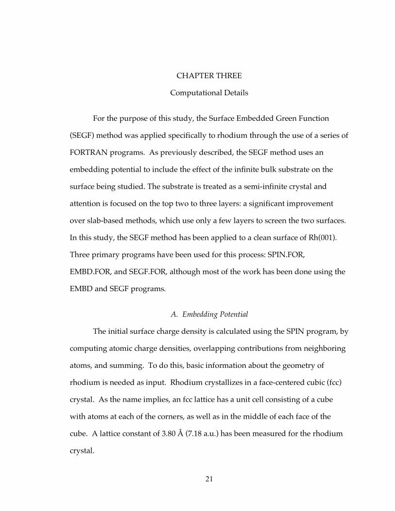
This study focuses on the (001) surface of rhodium. This being the case,
the surface is shown as Figure 3.2, with the basis vectors being defined from the
center of a corner atom to the center of the closest face atoms.
This geometric information is used as input for the SPIN program, which
computes the initial charge density for the SEGF program. The EMBD program
uses the bulk potential and additional structural information to produce the
embedding potential for the SEGF program. For this work, the rhodium bulk
muffin tin potential of Moruzzi, Janak, and Williams (MJW)23 was used. The
Fermi energy for rhodium is 0.341 Hartrees (9.29 eV) with respect to the average
23
Figure 3.2. Top view of Rh(001) demonstrating basis vectors.
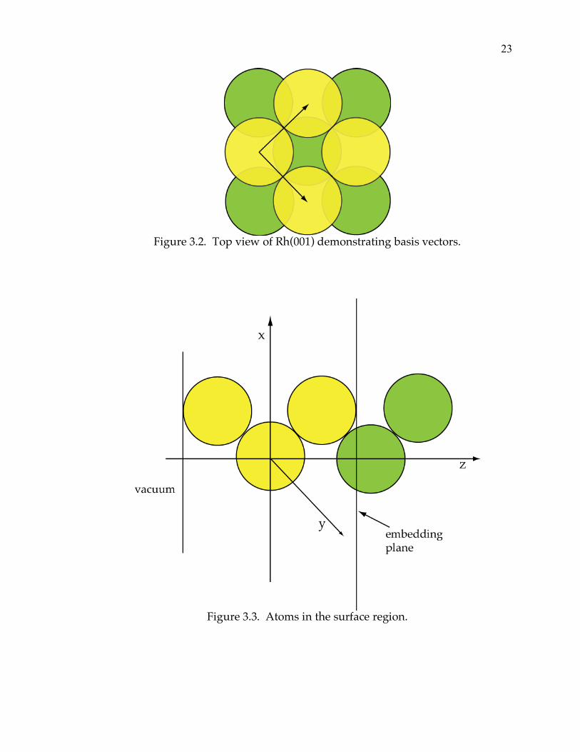
Figure 3.3. Atoms in the surface region.

24
interstitial potential. (Hartrees are the energy units used in the EMBD and SEGF
programs.) The embedding plane can be seen in Figure 3.3. The embedding
potential is the key ingredient for computing the self-consistent charge density
and densities of states.
In addition to producing the embedding potential, the EMBD program
can be used to calculate the bulk band structure. The bulk band structure was
calculated at several k points in order to compute the projected bulk band
structure (see section III.C). These will be discussed further in chapter 4.
B. Self-Consistent Charge Density
Once the embedding potential has been determined using the EMBD
program, it is used as an input to the SEGF program. The SEGF program then
iterates the charge density to self-consistency. This can be a lengthy process: for
Rh(001), over a thousand cycles were required for the charge density to
converge to a norm (root mean square of the charge difference vector) of 10-6
a.u. Once this was achieved, the charge density was considered converged. This
was accomplished by alternating between three cycles of simple mixing and ten
cycles of Broyden mixing. Other physical quantities were subsequently
computed from the converged results.
C. Bulk Band Structure and Projected Bulk Band Structure
Using the EMBD program, the bulk band structure can be calculated at
various k points within the Surface Brillouin Zone (SBZ). Since there is no
periodicity perpendicular to the surface, the three dimensional bulk Brillouin
zone must transform into the two-dimensional SBZ. Consequently, the bulk
bands (which all extend to the surface) must be labeled with only the two
25
components of the surface wavevector k. Where bands in the bulk could be
distinguished by their k
!component, at the surface they become band continua
plotted as a function of k (= k! ). For each k point, band energies were calculated
between 0 Ha and 0.42 Ha to ensure that the bottom of the valence band was
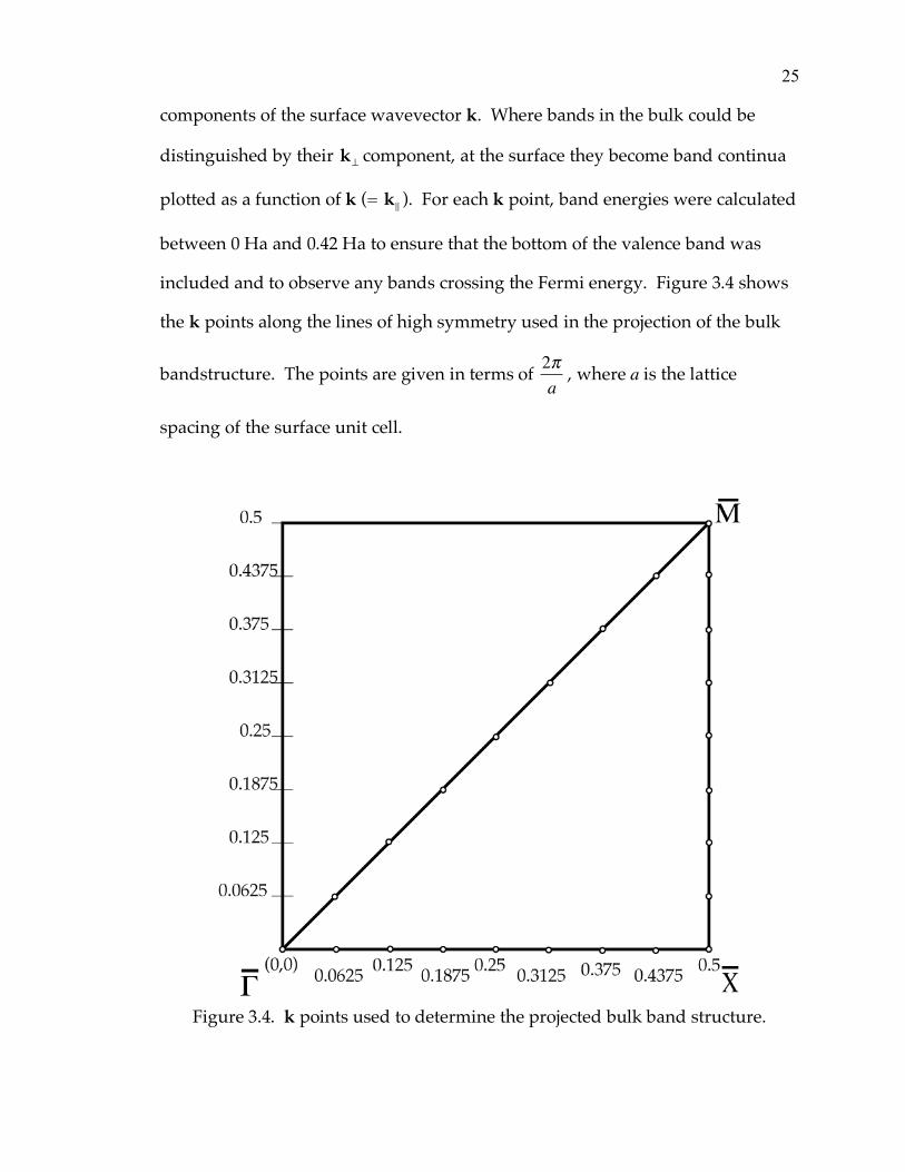
included and to observe any bands crossing the Fermi energy. Figure 3.4 shows
the k points along the lines of high symmetry used in the projection of the bulk
bandstructure. The points are given in terms of 2!a
, where a is the lattice
spacing of the surface unit cell.
Figure 3.4. k points used to determine the projected bulk band structure.

26
To construct the projected bulk band structure (PBBS), all bands were
analyzed for parity and to determine their energy minima and maxima. The
minima and maxima of different k points were then connected using a cubic
spline-fitting curve to illustrate the projected bulk band continua. The PBBS plot
can be used to identify surface states and surface resonances. In practice, bands
at additional k points were analyzed to better identify boundaries of various
band continua.
D. Density of States
The EMBD and SEGF programs can also be used in combination to
produce a density of states (DOS) plot. The EMBD program is used to produce
an embedding potential over the energy range of interest, but with energy points
located just above the real axis, instead of along the semi-circular contour used in
self-consistent cycles. The SEGF program is then run using the converged charge
density, to produce the density of states. At each k point the results are plotted,
and surface states and resonances are identified by sharp peaks in the DOS.
Typical DOS plots can be seen in Figures 4.9 – 4.11. Peak energies are next
plotted on the PBBS to identify surface states and surface resonances.
27
CHAPTER FOUR
Results and Analysis of Clean Rhodium
As discussed previously, crystalline rhodium’s structure is face-centered
cubic (fcc). For the Rh(001) surface, an embedding potential was produced from
an existing potential for the bulk atomic configuration. With this embedding
potential, three layers of surface atoms were effectively embedded onto an
infinite bulk substrate. The self-consistent surface charge density was computed,
and then used to study various physical properties. In this study, the work
function and core level shifts were computed and compared to experiment and
other calculated results. In addition, bulk band structures were calculated and
analyzed to produce the projected bulk band structure (PBBS) for the Surface
Brillouin Zone. Densities of states were also calculated and compared to the
PBBS to identify surface states and surface resonances.
A. Work Function
The work function is one of the more commonly calculated results, since it
is experimentally accessible and easy to compute. However, the accuracy of the
calculated work function is often viewed as a measure of the accuracy of the
calculation, since it depends sensitively on the arrangement of charge at the
surface. The work function for the (001) surface of rhodium was calculated to be
5.546 eV. As can be seen in Table 4.1, while this result does not correspond
closely to experimental values, it does compare favorably to other theoretical
values.

28
Xie and Scheffler25 and Cho and Sheffler31 have performed two density
functional theory (DFT) calculations using different approximations for the
exchange-correlation. The generalized gradient approximation (GGA) produced
a work function very close to experiment, while the local density approximation
(LDA) produced a work function in good agreement with the present results. It
is also worth noting that Gay et al.24 calculated a work function close to, but lower
than, experiment using a seven-layer self-consistent local-orbital method—
generally considered the least accurate method. Other calculated values are
generally higher than the experimental values, but in fairly good agreement with
Table 4.1. Comparison of experimental and theoretical work functions.
Method Result
Present SEGF result 5.55 eV
expt.- photoelectric effect28 4.92 eV
expt.- photoelectric effect29 4.98 eV
LAPW with LDA30 5.49 eV
7-layer LAPW with LDA25 5.30 eV
7-layer LAPW with GGA25 4.91 eV
9-layer LAPW with LDA31 5.26 eV
9-layer LAPW with GGA31 4.92 eV
7-layer SCLO24 4.8 eV
7-layer LMTO32 5.25 eV
9-layer pseudopotential33 5.57 eV
LAPW, Wigner interp.36 5.5 eV

29
the present SEGF result. The SEGF-calculated work function is in excellent
agreement with that produced by Morrison et al.33 using a nine-layer
pseudopotential. It also agrees very well with results by Feibelman and Hamann
using both the LAPW total energy30 method and the surface LAPW36 method.
There are competing views as to why most calculated work functions
deviate from experiment. One explanation pertains to the relaxation of the
outermost layer spacing. When Cho and Sheffler31 performed the two
calculations mentioned, they also considered the relaxation of the first surface
layer of Rh(001). Their results predicted a contraction of the outermost layer
spacing of about 3% using the LDA, and 2.8% using the GGA. The
pseudopotential method by Morrison et al.33 calculated a 3.22% contraction of the
top layer spacing.
For this reason, a second SEGF calculation of the electronic structure of
Rh(001) was performed. The parameters for this calculation were the same as in
the previous, except for a 3% contraction in the top surface layer spacing. The
resulting work function was calculated to be 5.563 eV, very close to the value
found by Morrison et al.,33 and not significantly different from the original SEGF
result.
There have also been experimental results that purport to measure a first
layer lattice expansion of about 1%34,39. Feibelman and Hamann30 argue that the
sample used in the low energy electron diffraction (LEED) measurements may
have been contaminated by a layer of hydrogen. However, there has been no
experimental evidence to support this view.

30
To consider the possible lattice expansion, the SEGF program was also run
for a Rh(001) surface with a 1% expansion of the surface spacing. The charge
density was converged, and a work function of 5.548 eV was determined. Thus,
contraction and expansion had no significant effect on the calculated work
function, so it is apparent that the SEGF method is robust enough not to be
affected by small perturbations of the geometry.
Hence, the discrepancy remains between experimental and computational
work functions. Among the possible explanations is some other type of surface
imperfection or impurity that alters the experimental value. There is also the
possibility that the top layer of the surface may be disordered, rendering
assumptions made in the surface calculations inaccurate.
Since the MT radius was reduced so that the expansion and contraction
would fit within the boundaries of the surface, the surface charge density was
also converged to self-consistency with the reduced MT radius, but using the
original geometry. The total energies were then compared, and the total energy
for the expanded surface was found to be 0.003 eV per unit cell higher than that
of the unrelaxed lattice. The contracted surface was found to have a total energy
that is 2.21 eV per unit cell lower than the unrelaxed surface. Thus, the current
results are consistent with the other theoretical predictions of a contracted layer
spacing.31,33
B. Surface Core-Level Shifts
There is often a difference in binding energy of the core level electrons in
the surface atoms as opposed to those in the bulk. This difference in energy is
called the surface core-level shift (SCLS). In general, there are three contributions

31
to the surface core-level shift (
�
!SCLS): a shift due to environmental effects (
�
!env ), a
shift due to a change in atomic configuration (
�
!conf ), and a relaxation shift (
�
!relax )
due to the screening of the core hole.
! = !env + !conf + !relax (4.1)
The environmental and configuration shifts together make up the initial
state effect (
�
!init ):
!init = !env + !conf (4.2)
The initial state effect is calculated using data from the SEGF program.
Once the charge density is converged, the potential at the top surface layer is
compared to that in the third layer, which essentially becomes part of the bulk
through embedding. The difference in the 3d5/2 eigenvalues is the initial state
contribution to the SCLS.
The environmental effect is calculated by running the SEGF program, but
calculating only the core levels and stopping short of running a full cycle. An
input potential is first created by overlapping charge densities and then solving
Poisson’s equation for a specific configuration (in this case 4d85s1). In this way,
no re-configuration of electrons at the surface is allowed, since the electron
configuration remains fixed. Then, comparing the first and third layers, the
environmental effect is found.
The configuration effect, also known as the chemical shift, is a result of the
rearrangement of surface electrons between atomic subshells. It can be
calculated by taking the (converged) initial state shift and subtracting the
environmental shift:
!conf = !init " !env . (4.3)

32
The relaxation shift, or final state effect, is a result of the different
screening properties of bulk and surface atoms. The final state effect is
calculated by placing a “hole” in the electron configuration at the first layer and
iterating to self-consistency. The same is then done for the third layer, and the
surface energies of the two systems are compared.
The environmental effect was calculated by creating a starting charge
density using an electron configuration of 4d85s1. The 3d5/2 energies were
compared at the first and third layers for the surface shift and the second and
third layers for the subsurface shift. For the environmental shift, a value of 215
meV towards decreased binding was calculated at the surface and 8 meV at the
subsurface.
The initial state shift was calculated using the converged SEGF surface
charge density. The one-electron potential in the top layer was somewhat less
attractive than the bulk, producing an initial shift towards decreased binding in
the amount of 667 meV for the 3d5/2 electron. In contrast, the subsurface layer
shifts towards increased binding by 95 meV.
With the initial state and environmental effects calculated, the shift due to
configuration changes can be found by taking the difference. A value of 452 meV
towards decreased binding is found at the surface, along with 103 meV towards
increased binding at the subsurface.
According to Ganduglia-Pirovano et al.,40 much of the surface core level
shift is a result of a surface d-band shift (SDBS). The SDBS to reduced binding
causes d to s charge transfer, resulting in a d orbital core shift that accounts for
much of the SCLS. There is a corresponding narrowing of the d-band which is
necessary for the surface to remain electrically neutral.
33
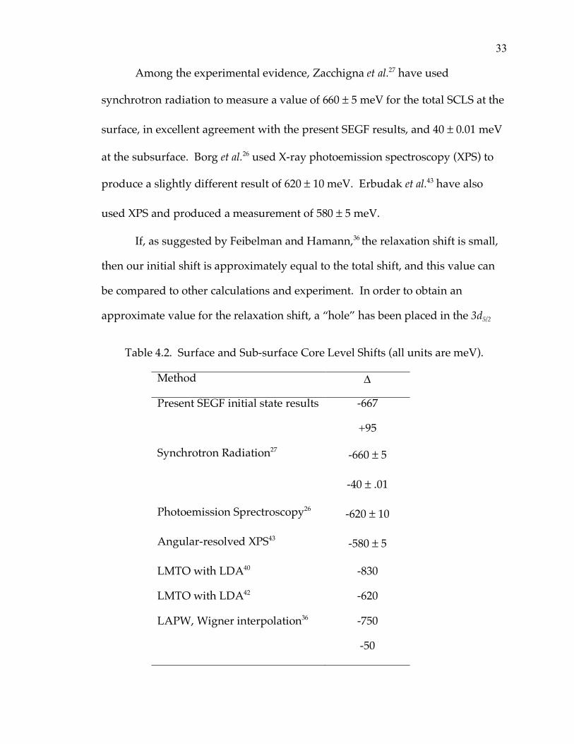
Among the experimental evidence, Zacchigna et al.27 have used
synchrotron radiation to measure a value of 660 ± 5 meV for the total SCLS at the
surface, in excellent agreement with the present SEGF results, and 40 ± 0.01 meV
at the subsurface. Borg et al.26 used X-ray photoemission spectroscopy (XPS) to
produce a slightly different result of 620 ± 10 meV. Erbudak et al.43 have also
used XPS and produced a measurement of 580 ± 5 meV.
If, as suggested by Feibelman and Hamann,36 the relaxation shift is small,
then our initial shift is approximately equal to the total shift, and this value can
be compared to other calculations and experiment. In order to obtain an
approximate value for the relaxation shift, a “hole” has been placed in the 3d5/2
Table 4.2. Surface and Sub-surface Core Level Shifts (all units are meV).
Method !
Present SEGF initial state results -667
+95
Synchrotron Radiation27 -660 ± 5
-40 ± .01
Photoemission Sprectroscopy26 -620 ± 10
Angular-resolved XPS43 -580 ± 5
LMTO with LDA40 -830
LMTO with LDA42 -620
LAPW, Wigner interpolation36 -750
-50

34
level of the surface layer and the calculation was re-converged. The results were
compared with similarly treated holes in the second and third layers. However,
since the unit cell is repeated continually, the hole is also repeated for all atoms
in the layer, resulting in an overestimate of the effect. When the core level
eigenvalues are compared, the top layer has shifted to 599 meV reduced binding
compared with the third layer eigenvalue. This value is a combination of all
contributions and is not just the relaxation shift. If this result is taken to be a
calculated total shift, it also is in fair to good agreement with the two
experimental measurements of the total core level shift (620 meV26 and 660
meV27).
Among other calculated results, Methfessel et al.42 report a total SCLS of
620 meV, in good agreement with the present findings and experiment.
Additionally, an approximate initial state shift of 580 meV and a relaxation shift
at 40 meV were calculated. Feibelman and Hamann36 calculated the total SCLS to
be 750 meV toward decreased binding at the surface and 50 meV at the
subsurface, while Ganduglia-Pirovano et al.40 calculated an SCLS of 830 meV
towards decreased binding.
C. Projected Bulk Band Structure
The projected bulk band structure (PBBS) is the projection of the bulk
energy spectrum onto the Surface Brillouin Zone (SBZ). It is constructed from
the bulk band structure for k points along high symmetry lines in the SBZ, as
shown in Figure 3.4. A bulk band structure is plotted for each k point and then
each band is evaluated for even and odd reflection symmetry across the high-
symmetry lines. The minimum and maximum energies for each band are then

35
determined. Figure 4.1 shows the bulk band structure at ! , with the energy set
to zero at the Fermi level. Note: The zone boundary occurs when
k!= 2"
a(# 0.875 a0
$1), where a is the bulk edge length.
Figure 4.1. Bulk band structure at ! [(0,0)] plotted as a function of k
!.
When the band structure is evaluated for adjacent k points, the bands
shift, as seen in Figure 4.2, the bulk band structure at (0.125, 0).
The bottom valence band is completely symmetric. Along the symmetry
lines, bands of the same parity cannot cross due to the Pauli exclusion principle.
At points of high symmetry, such as ! , there may be degeneracies and band
crossings due to the higher-order symmetry. Away from the high-symmetry
points, only the reflection symmetry across the symmetry lines is retained.
Figures 4.3 and 4.4 show the bulk band structure for the other two high-
symmetry points, X and M .

36
Figure 4.2. Bulk band structure at (0.125, 0) plotted as a function of k
!.
Figure 4.3. Bulk band structure at X [(0.5,0)] plotted as a function of k
!.

37
Figure 4.4. Bulk band structure at M [(0.5,0.5)] plotted as a function of k
!.
After the band structures have been calculated and the minimum and
maximum band energies determined, this information is combined to form the
PBBS. The maxima and minima are plotted in the SBZ and then the points are
connected using a cubic spline fit to produce the bulk energy band continua.
When necessary, additional k points have been evaluated to further clarify some
areas of band formation. For purposes of clarity, the PBBS for the ! X section of
the SBZ is shown in three different figures. Figure 4.5 displays the even-
symmetry bands and band gaps, and Figure 4.6 displays the odd-symmetry
bands and band gaps. The vertical lines represent continua of bulk bands of
even symmetry, while the horizontal lines represent bands of odd symmetry. In
these figures four symmetry gaps may be observed: three of even symmetry and
one odd. Figure 4.7 combines the previous figures to show the total PBBS for the

38
! X high-symmetry line. There are two absolute gaps displayed in this region.
Figure 4.5. PBBS of even symmetry for the ! X line in the SBZ. The vertical lines represent bands of even symmetry. There are three relative band gaps.

39
Figure 4.6. PBBS of odd symmetry for the ! X line in the SBZ. The horizontal lines represent bands of odd symmetry. There is one relative band gap.

40
Figure 4.7. PBBS for the ! X line in the SBZ. The horizontal lines represent bands of odd symmetry and vertical lines represent bands of even symmetry. There are two absolute band gaps.

41
Figu
re 4
.8.
PBBS
for t
he e
ntire
SBZ
. Ev
en a
nd o
dd sy
mm
etry
are
mar
ked
as p
revi
ousl
y no
ted.

42
Continuing with the rest of the SBZ, the PBBS for the X M and M ! high-
symmetry lines are produced. These are combined to produce the total PBBS, as
seen in Figure 4.8.
The PBBS in this study compares favorably to that produced by Eichler, et
al.41 for rhodium using a calculation incorporating pseudopotentials and an
iterative solution of the Kohn-Sham equations in the local density approximation
(LDA). The PBBS in Figure 4.8 also matches rather nicely with PBBS for iridium35
and platinum.8 Like rhodium, these are both fcc transition metals. Although
rhodium is a 4d metal and the others are 5d, the similarities in crystal structures
and numbers of valence electrons produce similar PBBS.
D. Densities of States
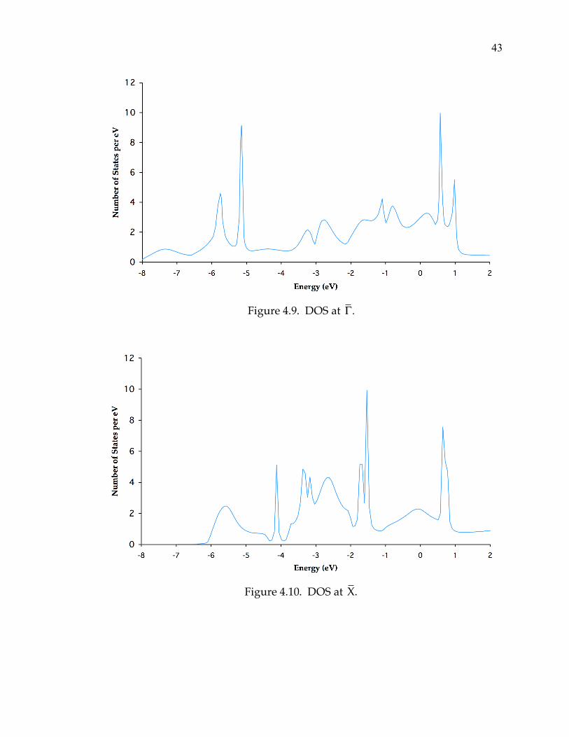
The densities of states (DOS) have been evaluated at each of the k points
shown in Figure 3.4. The peak position energies and wavevectors have been
plotted on the PBBS to identify the various surface states (SSs) and surface
resonances (SRs). Figures 4.9 through 4.11 are the DOS plots for the ! , X , and
M points of high symmetry. Figure 4.12 shows the position of all SS and SR
peaks with respect to the projected bulk bands.
Again with Ir(001)36 and Pt(001)8 as reference, the Rh(001) surface bands
are very similar to those computed for the other two surfaces. Platinum has one
more valence electron, and thus a higher Fermi energy; however, iridium is
isoelectronic to rhodium.
Very little experimental identification of rhodium surface states and
surface resonances has been performed. Morra et al.37 performed angle-resolved
photoemission experiments and found evidence for a strong surface state at
43
Figure 4.9. DOS at !.
Figure 4.10. DOS at X.
44
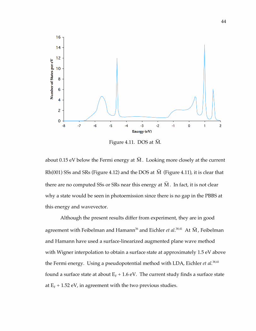
Figure 4.11. DOS at M.
about 0.15 eV below the Fermi energy at M . Looking more closely at the current
Rh(001) SSs and SRs (Figure 4.12) and the DOS at M (Figure 4.11), it is clear that
there are no computed SSs or SRs near this energy at M . In fact, it is not clear
why a state would be seen in photoemission since there is no gap in the PBBS at
this energy and wavevector.
Although the present results differ from experiment, they are in good
agreement with Feibelman and Hamann36 and Eichler et al.38,41 At M , Feibelman
and Hamann have used a surface-linearized augmented plane wave method
with Wigner interpolation to obtain a surface state at approximately 1.5 eV above
the Fermi energy. Using a pseudopotential method with LDA, Eichler et al.38,41
found a surface state at about EF + 1.6 eV. The current study finds a surface state
at EF + 1.52 eV, in agreement with the two previous studies.

45
Figu
re 4
.12.
PBB
S w
ith D
OS
poin
ts o
verla
yed.
Sur
face
stat
es a
re re
pres
ente
d by
solid
circ
les,
surf
ace
reso
nanc
es b
y op
en ci
rcle
s.

46
Feibelman and Hamann have argued30 that the experimental samples may
have been contaminated by an overlayer of hydrogen, which may account for the
difference between the present work and experiment. However, this suggestion
does not explain the theoretical results of Gay et al.,24 who find a surface state at
about 0.15 eV below the Fermi energy, exactly where the state was found
experimentally. As Feibelman and Hamann have stated, this is a point of concern
that should be further investigated.
E. Charge Density
The following figures are charge density plots of the Rh(001) surface
calculated using the SEGF program. They all represent the top three layers of the
sample. The vacuum is at the top in all figures. Figures 4.13 and 4.14 are total
charge density plots sampled over ten special k points. Figure 4.13 is taken
across the face of the cube; so it displays the expected five atom face
configuration. Figure 4.14 is taken across the cube diagonal and represents the
(110) plane; it makes clear the charge density between the “next nearest
neighbors.” As expected, the two plots show a sizable interstitial charge
everywhere, as would be expected for a metal. In each figure, the uppermost
charge density contour represents 0.009 e a0
3 . The average valence charge
density of 9 electrons per atom (0.049 e a0
3 ) is represented by the ninth charge
density contour.

47
Figure 4.13. Total charge density of the Rh(001) surface sampled over ten special k points. The minimum charge density is 0.009 electrons per cubic bohr radius ( e a
0
3 ), the maximum is 0.089 e a0
3 , and there are 17 contour lines.

48
Figure 4.14. Total charge density of the Rh(001) surface sampled over ten special k points. The minimum charge density is 0.009 e a
0
3 , the maximum is 0.089 e a0
3 , and there are 17 contour lines.

49
Figure 4.15 is a surface resonance at ! which lies 5.14 eV below the Fermi
level. The surface and subsurface appear to display dz2 orbital behavior with
some bonding between the two. Most of the valence charge lies in the top layer,
while very little resides in the third layer.
Figure 4.15. Valence charge density of the surface resonance of ! (0, 0) at EF – 5.14 eV. The minimum charge density is 0.002 radius e a
0
3 , the maximum is 0.042 e a
0
3 , and there are 21 contour lines.

50
Figure 4.16 is the charge density of the surface state at the (0.25,0) k point,
4.80 eV below the Fermi energy. It is in the lower absolute gap along the ! X
high-symmetry line. The bulk and subsurface exhibit dz2 orbital character.
There is less covalency at this surface state, perhaps representing some
antibonding behavior.
Figure 4.16. Valence charge density of the (0.25, 0) surface state at EF – 4.80 eV. The minimum charge density is 0.005 e a
0
3 , the maximum is 0.055 e a0
3 , and there are 26 contour lines.

51
Figure 4.17 is the charge density of the X surface state, which lies 4.12 eV
below the Fermi level. It is in the bottom absolute gap that occurs along both the
! X and X M high-symmetry lines. All three layers contribute to the surface
state, with the top two layers sharing some charge, and the subsurface displays
dxz,yz orbital character.
Figure 4.17 Valence charge density of the (0.5, 0) surface state at EF – 4.12 eV. The minimum charge density is 0.001 e a
0
3 , the maximum is 0.015 e a0
3 , and there are 29 contour lines.

52
The charge density of the surface state at 2.62 eV below the Fermi energy
at the (0.5, 0.0625) k point is displayed in Figure 4.18. It lies in a narrow absolute
gap in the middle of the bulk band continuum that exists along the X M high-
symmetry line. The subsurface and bulk layers exhibit dx2! y
2 orbital character
while the surface layer is dz2 . All three layers contribute to the surface valence
charge.
Figure 4.18. Valence charge density of the (0.5, 0.0625) surface state at EF – 2.62 eV. The minimum charge density is 0.005 e a
0
3 , the maximum is 0.105 e a
0
3 , and there are 21 contour lines.

53
Figure 4.19 shows the surface state at the (0.5, 0.25) k point which lies just
below the Fermi level (0.20 eV). All three layers contribute to the surface state
charge and exhibit dz2 orbital character.
Figure 4.19. Valence charge density of the (0.5, 0.25) surface state at EF – 0.20 eV. The minimum charge density is 0.002 e a
0
3 , the maximum is 0.042 e a0
3 , and there are 21 contour lines.
54
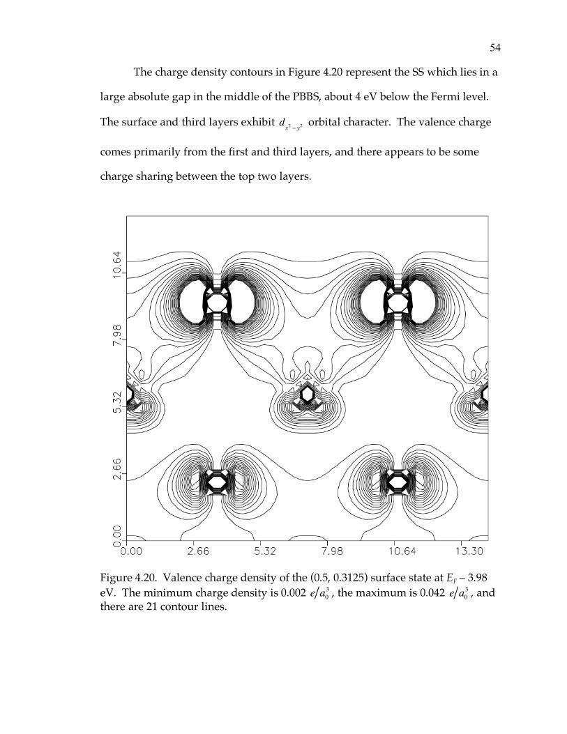
The charge density contours in Figure 4.20 represent the SS which lies in a
large absolute gap in the middle of the PBBS, about 4 eV below the Fermi level.
The surface and third layers exhibit dx2! y
2 orbital character. The valence charge
comes primarily from the first and third layers, and there appears to be some
charge sharing between the top two layers.
Figure 4.20. Valence charge density of the (0.5, 0.3125) surface state at EF – 3.98 eV. The minimum charge density is 0.002 e a
0
3 , the maximum is 0.042 e a0
3 , and there are 21 contour lines.

55
The SS at M , which lies 0.98 eV above the Fermi level, is very interesting,
as several band continua meet at this point. The charge density of this SS is
shown in Figure 4.21 and displays dyz,xz orbital character at all three layers.
Although all three layers are involved, the third layer appears to contribute the
most. As this state is above the Fermi level, it is unoccupied and should be
detectable by inverse photoemission.
Figure 4.21. Valence charge density of the (0.5, 0.5) surface state at EF + 0.98 eV. The minimum charge density is 0.0001 e a
0
3 , the maximum is 0.0061 e a0
3 , and there are 31 contour lines.

56
Figure 4.22 displays the charge density of the (0.3125, 0.3125) SS in the
absolute gap which lies 0.58 eV below the Fermi level. All three surface layers
exhibit dz2 orbital character and contribute to the valence charge.
Figure 4.22. Valence charge density of the (0.3125, 0.3125) surface state at EF – 0.58 eV. The minimum charge density is 0.002 e a
0
3 , the maximum is 0.42 e a
0
3 , and there are 21 contour lines.

57
Figure 4.23 is the charge density of the (0.1875, 0.1875) surface state at 3.92
eV below the Fermi level. The third layer appears to display dxz,yz orbital
character and the surface appears to display dz2 orbital character, while the
subsurface may be an admixture of orbitals. There is some covalency between
the layers and they all contribute to the charge.
Figure 4.23. Valence charge density of the (0.1875, 0.1875) surface state at EF – 3.92 eV. The minimum charge density is 0.005 e a
0
3 , the maximum is 0.055 e a
0
3 , and there are 11 contour lines.

58
Finally, Figure 4.24 is the charge density of the (0.0625, 0.0625) surface
state, which lies 3.03 eV below the Fermi level. All three layers exhibit dxz,yz
orbital character and can be seen to contribute charge, though the top layer
contributes very little, while the bottom two layers seem to show covalency.
Figure 4.24. Valence charge density of the (0.0625, 0.0625) surface state at EF – 3.03 eV. The minimum charge density is 0.0005 e a
0
3 , the maximum is 0.0105 e a
0
3 , and there are 11 contour lines.
The calculations presented are an important first step to understanding
the catalysis that occurs when NO and CO are placed atop the surface. It is

59
hoped that future experiments will examine the involvement of these SSs and
SRs in the catalytic activity of the surface.

60
CHAPTER FIVE
Conclusion The surface charge density for three layers of Rh(001) embedded on bulk
rhodium has been converged to self-consistency. Using the calculated charge
density, various electronic structural properties have been obtained. The
calculated work function compared favorably with other theoretical models, but
is in only fair agreement with experiment. Additional calculations were
performed to account for both lattice contraction and expansion, but the work
function was essentially unchanged. This model can be extended to other
surface geometries in order to resolve the discrepancy between theory and
experiment.
Components of the surface core-level shift (SCLS) were also calculated,
including the environmental and initial shifts, from which the configuration shift
was determined. These were in good agreement with both theory and
experiment. Our calculated initial state shift of 667 meV was in excellent
agreement with an experimental value of 660 ± 5 meV measured by Zacchigna et
al.27 Our attempt to calculate the relaxation shift was not as successful.
However, the current model could be used in conjunction with a 2 x 2 (or larger)
unit cell to better approximate the screening effect of a single atom, rather than a
plane of surface atoms.
The projected bulk band structure (PBBS) was constructed and densities of
states calculated and overlayed on the PBBS to identify surface states and surface

61
resonances. The structure of the PBBS is in good agreement with other models,
as well as those of iridium and platinum, which are closely related. While there
are few experimental studies with which to compare, the current calculations are
not in agreement with the experimental finding of an occupied surface state at
M .37 However, our results are in agreement with a theoretical study that
suggests that the experimental sample may have been contaminated with
hydrogen.30 The SEGF model has the capability of performing calculations with
impurities atop the metal surface, so it can be used to model a contaminated
surface if the geometry is known. Since rhodium is used as an industrial catalyst
for carbon monoxide and nitrogen oxide reduction, future studies could focus on
those reactions in hopes of improving both yield and efficiency.

62
REFERENCES
1J. E. Inglesfield, J. Phys. C 14, 3795 (1981). 2G. A. Benesh and J. E. Inglesfield, J. Phys. C 17, 1595 (1984). 3J. E. Inglesfield and G. A. Benesh, Phys. Rev. B 37, 6682 (1988). 4G. A. Benesh and J. E. Inglesfield, J. Phys. C 19, L539 (1986). 5G. A. Benesh and L. S. G. Liyanage, Phys. Rev. B 49, 17264 (1994). 6D. Gebreselasie, Ph.D. Dissertation, Baylor University, 1995 (unpublished). 7J. Sams, M.S. Thesis, Baylor University, 1987 (unpublished). 8G. A. Benesh, L. S. G. Liyanage, and J. C. Pingel, J. Phys.: Condens. Matter 2,
9065 (1990).
9G. A. Benesh and L. S. G. Liyanage, Surf. Sci. 261, 207 (1992). 10D. Wristers, M.S. Thesis, Baylor University, 1989 (unpublished). 11W. C. Bridgman, M.S. Thesis, Baylor University, 1992 (unpublished). 12V.R. Dhanak, A. Baraldi, G. Comelli, K.C. Prince, and R. Rosei, Phys. Rev. B 51,
1965 (1995). 13N. W. Ashcroft and N. D. Mermin, Solid State Physics, (Saunders College,
Philadelphia, 1976). 14P. Hohenberg and W. Kohn, Phys. Rev. 136, B864 (1964). 15W. Kohn and L. J. Sham, Phys. Rev. 140, A1133 (1965). 16A. Zangwill, Physics at Surfaces, (Cambridge University Press, Cambridge,
1988). 17S. Crampin, J. B. A. N. van Hoof, M. Nekovec, and J. E. Inglesfield, J. Phys.:
Cond. Matter 4, 1475 (1992). 18J. B. Pendry, Low Energy Electron Diffraction, (Academic Press, London, 1974). 19M. Weinert, J. Math. Phys. 22, 2433 (1981).

63
20C. G. Broyden, Math. of Comp. 19, 577 (1965). 21D. D. Johnson, Phys. Rev. B 38, 12807 (1988). 22David Vanderbilt and Steven G. Louie, Phys. Rev. B 30, 6118 (1984).
23V. L. Moruzzi, J.F. Janak, and A.R. Williams, Calculated Electronic Properties of Metals (Pergamon, New York, 1978).
24J.G. Gay, J.R. Smith, and F.J. Arlinghaus, Phys. Rev. B 25, 643 (1982).
25Jianjun Xie and Mathias Scheffler, Phys. Rev. B 57, 4768 (1998).
26A. Borg, C. Berg, S Raaen, and H.J. Venvik, J. Phys.: Cond. Matter 6, L7 (1994). 27M. Zacchigna, C. Astaldi, K.C. Prince, M. Sastry, C. Comicioli, M. Evans, R.
Rosei, C. Quaresima, C. Ottaviani, C. Crotti, M. Matteuci, and P. Perfetti, Phys. Rev. B 54, 7713 (1996).
28American Institute of Physics Handbook, 3rd ed. (McGraw-Hill, New York, 1972), p.
9-176. 29CRC Handbook of Chemistry and Physics, 84th ed.(CRC Press, Boca Raton, 2003), p.
12-130. 30P.J. Feibelman, D.R. Hamann, Surface Science 234, 377 (1990). 31Jun-Hyung Cho and Matthias Scheffler, Phys. Rev. Letters 78, 1299 (1997). 32M. Methfessel, D. Hennig, and M. Scheffler, Phys. Rev. B 46, 4816 (1992). 33Ian Morrison, D.M. Bylander, and Leonard Kleinman, Phys. Rev. Lett. 71, 1083
(1993). 34S. Hengrasmee, K.A.R. Mitchell, P.R. Watson, and S.J. White, Can. J. Phys. 58,
200 (1980). 35O. Bisi, C. Calandra, and F. Manghi, Sol. State Comm. 23, 249 (1977). 36Peter J. Feibelman and D.R. Hamann, Phys. Rev. B 28, 3092 (1983). 37R.M. Morra, F.J.D. Almeida, and R.F. Willis, Phys. Scr. 41, 594 (1990). 38A. Eichler, J. Hafner, J. Furthmüller, and G. Kresse, Surf. Sci. 346, 300 (1996). 39W. Oed, B. Dötsch, L. Hammer, K. Heinz, and K. Müller, Surf. Sci., 207, 55
(1988).

64
40M.V. Ganduglia-Pirovano, V. Natoli, M.H. Cohen, J. Kudrnovsky´, I. Turek, Phys. Rev. B 54, 8892 (1996).
41A. Eichler, J. Hafner, G. Kresse, and J. Furthmüller. Surf. Sci. 352-354, 689 (1996). 42M. Methfessel, D. Hennig, M. Scheffler, Surf. Rev. and Lett. 2, 197 (1995). 43M. Erbudak, P. Kalt, L. Schlapbach, and K. Bennemann, Surf. Sci. 126, 101
(1983).
Recommended