lable at ScienceDirect

Progress in Biophysics and Molecular Biology 107 (2011) 74e80

Contents lists avai

Progress in Biophysics and Molecular Biology

journal homepage: www.elsevier .com/locate/pbiomolbio

Review

Considerations for the use of cellular electrophysiology modelswithin cardiac tissue simulations

Jonathan Cooper a,*, Alberto Corrias a,1, David Gavaghan a, Denis Noble b

aOxford University Computing Laboratory, University of Oxford, Wolfson Building, Parks Road, Oxford OX1 3QD, UKbDepartment of Physiology, Anatomy & Genetics, University of Oxford, Oxford, UK

a r t i c l e i n f o

Article history:Available online 15 June 2011

Keywords:Cardiac electrophysiologyModel interfacesCellMLChaste

* Corresponding author.E-mail addresses: jonathan.cooper@comlab.ox.ac.

edu.sg (A. Corrias), david.gavaghan@comlab.ox.ac.ukdpag.ox.ac.uk (D. Noble).

1 Present address: Division of Bioengineering, NatiSingapore.

0079-6107/$ e see front matter � 2011 Elsevier Ltd.doi:10.1016/j.pbiomolbio.2011.06.002

a b s t r a c t

The use of mathematical models to study cardiac electrophysiology has a long history, and numerouscellular scale models are now available, covering a range of species and cell types. Their use to studyemergent properties in tissue is also widespread, typically using the monodomain or bidomain equationscoupled to one or more cell models. Despite the relative maturity of this field, little has been writtenlooking in detail at the interface between the cellular and tissue-level models. Mathematically this isrelatively straightforward and well-defined. There are however many details and potential inconsis-tencies that need to be addressed, in order to ensure correct operation of a cellular model within a tissuesimulation. This paper will describe these issues and how to address them.

Simply having models available in a common format such as CellML is still of limited utility, withsignificant manual effort being required to integrate these models within a tissue simulation. We willthus also discuss the facilities available for automating this in a consistent fashion within Chaste, ourrobust and high-performance cardiac electrophysiology simulator.

It will be seen that a common theme arising is the need to go beyond a representation of the modelmathematics in a standard language, to include additional semantic information required in determiningthe model’s interface, and hence to enhance interoperability. Such information can be added as meta-data, but agreement is needed on the terms to use, including development of appropriate ontologies, ifreliable automated use of CellML models is to become common.

� 2011 Elsevier Ltd. All rights reserved.

Contents

1. Introduction . . . . . . . . . . . . . . . . . . . . . . . . . . . . . . . . . . . . . . . . . . . . . . . . . . . . . . . . . . . . . . . . . . . . . . . . . . . . . . . . . . . . . . . . . . . . . . . . . . . . . . . . . . . . . . . . . . . . . . . .742. Issues to consider . . . . . . . . . . . . . . . . . . . . . . . . . . . . . . . . . . . . . . . . . . . . . . . . . . . . . . . . . . . . . . . . . . . . . . . . . . . . . . . . . . . . . . . . . . . . . . . . . . . . . . . . . . . . . . . . . . 75

2.1. Identification of model components . . . . . . . . . . . . . . . . . . . . . . . . . . . . . . . . . . . . . . . . . . . . . . . . . . . . . . . . . . . . . . . . . . . . . . . . . . . . . . . . . . . . . . . . . . . . . 752.2. Inconsistencies when connecting models . . . . . . . . . . . . . . . . . . . . . . . . . . . . . . . . . . . . . . . . . . . . . . . . . . . . . . . . . . . . . . . . . . . . . . . . . . . . . . . . . . . . . . . . 762.3. Issues for generic simulation software . . . . . . . . . . . . . . . . . . . . . . . . . . . . . . . . . . . . . . . . . . . . . . . . . . . . . . . . . . . . . . . . . . . . . . . . . . . . . . . . . . . . . . . . . . . 77

3. Example simulation . . . . . . . . . . . . . . . . . . . . . . . . . . . . . . . . . . . . . . . . . . . . . . . . . . . . . . . . . . . . . . . . . . . . . . . . . . . . . . . . . . . . . . . . . . . . . . . . . . . . . . . . . . . . . . . . . 784. Discussion and conclusions . . . . . . . . . . . . . . . . . . . . . . . . . . . . . . . . . . . . . . . . . . . . . . . . . . . . . . . . . . . . . . . . . . . . . . . . . . . . . . . . . . . . . . . . . . . . . . . . . . . . . . . . . . 79

Role of the funding source . . . . . . . . . . . . . . . . . . . . . . . . . . . . . . . . . . . . . . . . . . . . . . . . . . . . . . . . . . . . . . . . . . . . . . . . . . . . . . . . . . . . . . . . . . . . . . . . . . . . . . . . . . 80Editors’ note . . . . . . . . . . . . . . . . . . . . . . . . . . . . . . . . . . . . . . . . . . . . . . . . . . . . . . . . . . . . . . . . . . . . . . . . . . . . . . . . . . . . . . . . . . . . . . . . . . . . . . . . . . . . . . . . . . . . . . . 80Acknowledgements . . . . . . . . . . . . . . . . . . . . . . . . . . . . . . . . . . . . . . . . . . . . . . . . . . . . . . . . . . . . . . . . . . . . . . . . . . . . . . . . . . . . . . . . . . . . . . . . . . . . . . . . . . . . . . . . . 80References . . . . . . . . . . . . . . . . . . . . . . . . . . . . . . . . . . . . . . . . . . . . . . . . . . . . . . . . . . . . . . . . . . . . . . . . . . . . . . . . . . . . . . . . . . . . . . . . . . . . . . . . . . . . . . . . . . . . . . . . . 80

uk (J. Cooper), alberto@nus.(D. Gavaghan), denis.noble@

onal University of Singapore,

All rights reserved.

1. Introduction

Computational modelling of cardiac electrophysiology hasdeveloped extensively over the last 50 years at all spatial scales.Numerous models at the cellular scale are now available, covering

J. Cooper et al. / Progress in Biophysics and Molecular Biology 107 (2011) 74e80 75

a range of species, cell types, and experimental conditions. Aswell asbeing used to study cellular scale phenomena, these models arefrequently also embeddedwithin a framework that describes cardiactissue, in order to investigate the propagation of electrical activitythat gives rise to the heartbeat. Such emergent behaviour at thetissue level can be very effectively modelled (Clayton et al., 2010).

With its long history, this field is relatively mature. Many of thecellular level models have been curated and are available ina standard computer-readable format from the CellML modelrepository (Lloyd et al., 2008), providing easy access to checkedencodings of the model equations. Several tissue-level simulationenvironments are also available (Niederer et al., in press). Howeverdespite this, little has beenwritten looking in detail at the interfacebetween these levels. Perhaps this is because, as we shall describeshortly, this interface is relatively straightforward and well-definedfrom a mathematical point of view. However, in order to ensurecorrect operation of a cellular level model within a tissue simula-tion, there are many details and potential inconsistencies that mustbe taken into account and addressed.

Tissue-level cardiac electrophysiology is usually modelled usingthe bidomain equations (or themonodomain simplification thereof).These consist of two partial differential equations (PDEs) describingthe intracellular and extracellular potential fields (fi and fe) throughthe cardiac tissue as a reactionediffusion system, coupled at eachpoint in space with a system of ordinary differential equations(ODEs) representing the concentrations of ions andother variables atthe cellular level (see, for example, Keener and Sneyd, 1998). Let Udenote the region occupied by the cardiac tissue. In the para-boliceelliptic formulation, which describes fe and the trans-membrane voltage Vm ¼ fi � fe, the bidomain equations are then

c

�Cm

vVm

vtþ Iionðu;VmÞ

�� V$ðsiVðVm þ feÞÞ ¼ IðvolÞi ; (1a)

V$ððsi þ seÞVfe þ siVVmÞ ¼ �IðvolÞtotal ; (1b)

and for each point in U;vuvt

¼ f ðu;VmÞ; (1c)

where (1a) and (1b) describe the spatial and temporal evolution ofthe electrical potentials, and (1c) describes the remaining cellularlevel behaviour. Here si is the intracellular conductivity tensor, se isthe extracellular conductivity tensor, c is the surface area to volumeratio, Cm is the membrane capacitance per unit area, u is a set ofcell-level variables (such as gating variables, ion concentrations,etc.), and Iion h Iion(u, Vm) is the transmembrane ionic current persurface area. IðvolÞtotal ¼ IðvolÞi þ IðvolÞe , where the source terms IðvolÞi andIðvolÞe are the intra- and extracellular stimuli per unit volume.Appropriate boundary and initial conditions must also be applied;see (Pathmanathan et al., 2010a) for details.

In this paper, we examine three classes of issues concerning theinteroperability of CellML models of cellular electrophysiologywithin cardiac tissue simulations, and indicate possible strategiesto address each of them.

The first class of issues arises from the fact that the cellularmodels available in the CellMLmodel repository are not formulatedas components of a tissue model, but represent entities somewherebetween an isolated cell and a patch of cell membrane. They thusdo not provide straightforward definitions of the terms Iion and f asthey appear in (1). Rather, their equations appear in the form

dVm

dt¼ � Iionðu;VmÞ þ Istim

Cm; (2a)

dudt

¼ f ðu;VmÞ; (2b)

or a variation thereof. The first challenge is therefore to identify therelevant variables within the cell model for coupling to the tissuemodel, and extract the necessary equations. This is the topic ofSection 2.1.

The next class of issues, treated in Section 2.2, is that of incon-sistencies between the models being connected. This may arisethrough differing use of units, from variations in how the modelsare structured, or from differences in parameter values. The finalclass of issues we address, in Section 2.3, are those faced by soft-ware that is intended to be generic enough to be able to deal withdifferent cell types. A sample simulation, illustrating the impor-tance of addressing these issues correctly, is presented in Section 3.

These issues are of particular importance to those seeking toexploit the full potential of having cellular models available ina standard language such as CellML, by being able to reuse thesemodels within tissue simulations without significant manual effort.For each issue, we therefore also describe the support available inChaste (Pitt-Francis et al., 2009), via the PyCml software (Cooper,2009; Garny et al., 2008), for automatically addressing it whenprocessing a suitably annotated cell model. This allows the trans-parent inclusion of any cell model represented in CellML withina tissue simulation. The cardiac portion of Chaste is a powerful,efficient, parallel and well-engineered monodomain/bidomainsolver. Chaste is open-source and available for download at http://web.comlab.ox.ac.uk/chaste/. All of the functionality described inthis paper is present in the version 2.2 release.

We conclude in Section 4 by identifying common threads arisingfrom these issues, and discuss some of the wider implications forthe computational modelling field.

2. Issues to consider

The main focus of this paper is on the interfaces betweencellular and tissue-level models as systems of equations. Firstlyhowever, it must be noted that the choice of numerical scheme forsolving the equations also has an impact on this interface. Thisquestion has been investigated in some detail elsewhere and sowillnot be addressed here. For example, where and how in the spatialdomain the cellular models are evaluated can have a significantimpact on the accuracy of certain features of tissue simulations,such as the conduction velocity (Pathmanathan et al., 2011). Thechoice of stimulus currents is also important, and incompatibilitiescan arise from mixing formulations (Pathmanathan et al., 2010a).

2.1. Identification of model components

The first class of issues is concerned with the need to identifythose portions of the cellular model which form the interface to thetissue model. This requires being able to handle variations in modelvariable naming conventions (different authors use different namesfor key quantities) and also variations in how the model equationsare structured in the CellML encoding of the model. These onlycause difficulty when automating the reuse of models e if codingup the cellular model ‘by hand’ within a tissue simulator, therelevant portions are readily identified by eye.

The cellular model variables in (2) that form the interface to (1)are Vm, Iion, and Istim. Since this is a small set of quantities, onemightfirst consider simply testing for all names known to be used.Besides being prone to failure on new models that might usea novel nomenclature, this approach also requires testing fora surprising number of alternatives, and may for some modelsidentify incorrect variables, particularly in the case of Iion. The

Table 1Names used for key variables, and units used for ionic currents, in a small sample ofcellular models.

Model Componentname

Vm Istim Cm Units ofcurrents

DiFrancesco and Noble (1985) Membrane V i_pulse C nALuo and Rudy (1991) Membrane V I_stim C mA/cm2

Dokos et al. (1996) Membrane E N/A C pANoble et al. (1998) Membrane V i_Stim Cm nAJafri et al. (1998) Membrane V I_stim Cm mA/mm2

Viswanathan et al. (1999) Membrane V I_st Cm mA/mFMatsuoka et al. (2003) Membrane Vm i_ext Cm pAHund and Rudy (2004) Cell V i_Stim Acap mA/mFMahajan et al. (2008) Cell V i_Stim N/A mA/mFStewart et al. (2009) Membrane V N/A Cm pA/pF

J. Cooper et al. / Progress in Biophysics and Molecular Biology 107 (2011) 74e8076

multiplicity of options derives in part from the structure of CellML,in which models are decomposed into multiple components as anaid to reuse (Lloyd et al., 2004). There may thus be variation in bothcomponent names (typically cell or membrane are used for theexternal interface of themodel) and variable names. Common casesfor the latter include V, E, or Vm for Vm, and i_Stim, I_st, or i_pulsefor Istim, with variations in capitalisation also, as can be seen inTable 1. Identification of Iion is further complicated by variations inthe structure of the model equations, described in more detail inSection 2.2. In particular, there is often not a single variable for Iionin the model; rather it is implicit as a sum of component currentswithin the equation for dVm/dt. Hence analysis of the equation isrequired for robust automatic identification of this term, sincematching purely on variable names could potentially includecurrents which are internal to the cell, rather than only the trans-membrane currents comprising Iion.

Some manual configuration for each model is thus required fora truly robust solution. While this could be done using a separateconfiguration file (as was done in earlier Chaste releases) a betterand more extensible approach is to annotate model variables usingterms from a suitable ontology, building on the CellML metadataframework (Beard et al., 2009). The ontology provides standardisednames for important quantities, eliminating the variation innaming. Chaste currently uses its own mini-ontology for naming,which consists of a short list of identifiers built in to the software.2

However, it is intended to work towards a community standard, sothat models available from the CellML repository are pre-annotatedand ready to use directly.

However, annotating every variable does introduce an addi-tional task, whether for the model author, curator, or user. Toreduce this burden, PyCml is capable of analysing the modelmathematics to identify most of the interface. Only Vm and Istim arerequired to be explicitly identified. From these, we can determineIion as described in the next section. Finding the derivatives definedin the model is straightforward, and so extraction of du/dt simplyrequires ignoring dVm/dt. The subsidiary equations in the modelcan then be analysed to determine which are required incomputing du/dt and Iion, and suitable Cþþ code generated for usein Chaste (Cooper, 2009).

2.2. Inconsistencies when connecting models

A commonproblem arising in anymodel coupling exercise is theexistence of incompatibilities between the component models, dueto differing conventions or methodologies followed in developingthe constituent pieces. Three categories of such incompatibilitieswere defined by Terkildsen et al. (2008) as unit, structural, andparameter inconsistencies. These can usefully be applied in ourscenario, although frequently multiple types of inconsistency occurtogether.

The simplest case to resolve is that of unit inconsistencies. Theseoccur when the cellular and tissue-level models use differentphysical units for the same quantity. A common example is therepresentation of time, which is generally measured in eithermilliseconds (as in Chaste) or in seconds. In the latter casea conversion is required; it is a straightforward scaling in this casesince the dimensions match. Since all quantities in a CellML modelmust be explicitly associated with their units, it is possible to checkautomatically that the cellular model is internally consistentand add suitable conversions at component interfaces (Cooper andMcKeever, 2008). (If the cellular model is not internally consistent,

2 See https://chaste.comlab.ox.ac.uk/chaste/tutorials/release_2.2/ChasteGuides/CodeGenerationFromCellML.html for more details.

no conversions can be performed reliably, and the model must becorrected to ensure correct behaviour.) The interface to the tissuemodel can be addressed using the same functionality, by addinga new component to the CellML model containing variables in theunits required by the tissue model, and connecting these to thecorresponding variables in the cellular model. The tissue modelthen interacts only with this new interface component.

Other quantities at the interface must also be given in consistentunits. For Vm we know of no model that does not use millivolts(mV), but for ionic currents the situation is more complex due tothe existence of structural inconsistencies. These refer to differencesin how the biological system is represented by the mathematicalequations. There are three different conventions used in cellularmodels for representing transmembrane ionic currents. The first isto use whole-cell current, which is expressed in (multiples of)Amperes (A) (e.g. Noble et al., 1998). Alternatively the current maybe normalised, either by the cell membrane surface area (e.g. Luoand Rudy, 1991), or by its capacitance (e.g. Stewart et al., 2009),leading to units dimensions of A/m2 or A/F respectively. If thecellular and tissue-level models use different conventions, a simplescaling conversion is impossible. Furthermore, where normal-isation is employed, parameter inconsistencies may also play a role,with the cellular and tissue models using different estimates for thesame biological quantity (whether cell surface area or membranecapacitance).

Fortunately, we can make use of the parameter inconsistency toperform a suitable conversion for ionic currents into the unitsexpected by Chaste, mA/cm2, automatically. The three cases are asfollows.

1. Cellular model uses current per unit area (A/m2). These are thesame dimensions as used by Chaste for the tissuemodel, and soa simple scaling is sufficient.

2. Cellular model uses current per unit capacitance (A/F). In thiscase we note that the units of the ionic current are dimen-sionally equivalent to those for dVm/dt, and so the equation fordVm/dt should not include a scaling by Cm as in (2) e this isalready incorporated into the currents. We thus need only tochange the normalisation by scaling using Chaste’s estimate forthe membrane capacitance, measured in mF/cm2, to obtaincurrents in the expected dimensions.

3. Cellular model uses whole-cell current (A). Ideally, theconversion should be done by dividing by the (electricallyactive) cellular surface area defined by the cellular model.However, this information is not always available. Instead, weestimate it using the membrane capacitance, which is given inpure capacitance units (F) within the cellular model, but inmF/cm2 by the tissue model. Since these are conceptuallysupposed to represent the same quantity, the ratio of the twoyields an estimate of the electrically active area. Hence the only

J. Cooper et al. / Progress in Biophysics and Molecular Biology 107 (2011) 74e80 77

additional manual effort required in this case is annotation ofCm in the same way as for Vm. Note that this also assumes thatthe cellular model represents a single cell, and hence does notapply to models such as that of DiFrancesco and Noble (1985)which consider a multicellular preparation. In such cases,specific configuration is required.

If the tissue model uses a different convention from that used inChaste, similar conversions can be applied.3

There are further structural inconsistencies involved in theconnection of ionic currents between cellular and tissue level. Thefirst concerns the intracellular stimulus current, given by IðvolÞi inthe tissue model and Istim in the cellular model. Within Chaste, theformer is measured in mA/cm3 and the latter in mA/cm2, as is Iion.When the cellular model is being used in a tissue simulation,dVm/dt is not evaluated, and so Istim is not required there. However,for models such as that of Hund and Rudy (2004) which assign thestimulus current to particular ionic species in order to conservecharge, Istim is still used in computing du/dt. It must therefore becalculated as Istim ¼ IðvolÞi =c, where c is given in cm�1.

A particular advantage we have observed of performing theseconversions is that it reduces the amount of per-model ‘tweaking’required to achieve a successful tissue simulation. For example, thesame stimulus can now be applied by Chaste to produce an actionpotential in each of a sample of 32 cellular models. This is in starkcontrast to the default stimuli coded in the models, which varysignificantly.

Secondly, as we have alluded to already, the form of Equation(2a) can vary significantly. The convention followed by the majorityof cell models, and expected by Chaste, is for (4) to have the form

dVm

dt¼ � I1 þ.þ In þ Istim

Cm; (3)

whence the input to (1), Iion, is implicit and given by Iion¼ I1þ.þ In.The CellML versions of some models (e.g. Priebe and Beuckelmann,1998) introduce intermediate equations, for example dVm/dt ¼dVdt, dVdt ¼ �Itot, Itot ¼ I1 þ . þ In þ Istim. Other models (e.g.Mahajan et al., 2008) use the opposite sign for the currentscomprising Iion, whereas others (e.g. Jafri et al., 1998) instead invertjust Istim. Each of these variations can be automatically accounted forby PyCml, by analysing the model equations in the following steps.

1. Firstly, the currents forming Iion must be identified. This is doneby examining the variables appearing in (2a) and selectingthose with suitable units (excluding Istim). There are a fewsubtleties to this. If Istim is defined in themodel (i.e. it is not self-excitatory) then ‘suitable units’ means dimensionally equiva-lent to the units of Istim. Otherwise, the dimensions could beany of the three options for ionic currents discussed above.Once Iion has been identified, the convention actually used inthe model can be determined.The equations defining the model are thus systematicallysearched, starting from the definition of dVm/dt, for variableswith suitable units. If any are found, the sum of these (with theexception of Istim) is considered to be Iion. If none are found atfirst, the definitions of variables occurring in this equation arethen searched; if no suitable variables are found, the definitions

3 This approach to units conversions is conceptually similar to the process of non-dimensionalisation, in which quantities intrinsic to a system are used to scale theequations, yielding a new system using only dimensionless variables. While thistechnique is common in mathematical biology, it has not generally been applied inphysiological modelling; perhaps due both to the complexity of the models anda desire to keep parameters in physical units.

of variables occurring in those definitions are searched, and soon. The search is performed in this fashion in order to ensurethat currents are not double-counted, by including botha variable representing a sum of currents and the variablesrepresenting the individual currents included in the sum.One complication is that A/F is dimensionally equivalent to mV/ms, and so if intermediate equations are used, a variable such asdVdt could be mistakenly identified as an ionic current, despitethemodel using (say) thewhole-cell current convention. If Istim isnot present (and so the convention used is unknown), the searchis thus performed first with A/F excluded from the units options,stopping after two levels of definitions have been examined. Thisassumes that ionic currents will occur either in the equationdefining dVm/dt, in one of the equations defining variablesoccurring therein, or in the definitions of variables occurring inthose equations. A model would need to be structured veryunusually to break this assumption, which is made partly forefficiency, but primarily to guard against thepossibilityof featureslocated deeper within the equations being misidentified ascurrents, e.g. if an ionic current was defined by dividing some-thing measured in amps by a capacitance. No existing models doso as far as we are aware. If no suitable currents are found, thesearch is restarted with A/F included, and no early termination.A further complication is that Istim may occur within the defi-nition of currents identified as part of Iion (this can occur ifintermediate equations are used, or with conservative cellmodels). A check for this case is made when generating thecode for Iion, and if Istim is found, it is replaced by zero.

2. Secondly, the sign of Iion must be checked. Since PyCml alreadyincludes the ability to evaluate portions of a CellML model(Cooper, 2009), we can utilise this, faking the values assigned tovariables, to compute the sign of Iion by evaluating the right-hand side of (2a). Each of the currents identified in step 1 is(temporarily) assigned the value 1, as are other time-varyingvariables.4 If dVm/dt evaluates strictly positive, Iion is thenconsidered to be negated with respect to (3).

3. Finally, if it is present, the sign of Istim must be determined.Again this can be deduced by fake evaluation of (2a), but withdifferent values assigned to the variables. In this case, Istim is setto 1, other ionic currents are set to 0, and all other time-varyingvariables are set to 1. The stimulus is then negated (ascompared with (3)) if dVm/dt evaluates strictly positive.

2.3. Issues for generic simulation software

Other issues are faced by software such as Chaste which isintended to be generic, dealing with models of different cell types,and providing facilities for both single-cell and tissue-level simu-lation. The primary example concerns identification of the intra-cellular stimulus Istim. This will appear in models of ventricularcells, but generally not in self-excitatory cells such as from the sino-atrial node. If no stimulus is found, and the model representsa ventricular cell, processing software should report an error sincethis indicates that the stimulus has not been suitably annotated (asdescribed in Section 2.1). Otherwise, the stimulus current would beconsidered as part of Iion, and so an additional stimulus would beapplied to the cellular model, leading to incorrect results.

If, however, the cellular model represents a self-excitatory cell, itmay not contain a stimulus current, and so no error should be

4 Constant variables retain their values given in the model, in order to account forpathological cases, not seen in any models thus far, such as dVm/dt ¼ X$Iion/Cm withX ¼ �1.

J. Cooper et al. / Progress in Biophysics and Molecular Biology 107 (2011) 74e8078

reported in this case. (It should be noted that it is not an error ifa self-excitatory cell does contain a stimulus e a Purkinje cell mayexhibit both spontaneous and paced behaviour in vivo, and somemodels (e.g. Sampson et al., 2010) therefore consider both activi-ties.) Hence annotation of the model itself is required (or somealternative method of configuration) to indicate the type of cellbeing modelled, and hence whether to expect a stimulus current.

Various other technical issues, not central to the thrust of thispaper, may also be considered. For example, we also allow meta-data annotations that specify minimum and maximum possiblevalues for variables (e.g. to specify a probability that must liebetween zero and one, or a concentration that must be positive).Including these enables Chaste to check during a simulationwhether a variable has gone out of range, and terminate thesimulation early with an error if this occurs. Such a situation istypically due to parameters chosen for the numerical method beingunsuitable.

3. Example simulation

To demonstrate the functionality available in Chaste foraddressing the issues described above, proof-of-concept simulationresults are presented here (a video from a sample simulation ispresent in the supplementary material at doi:10.1016/j.pbiomolbio.2011.06.002; input files for this simulation can be found at http://www.cs.ox.ac.uk/chaste/publications/2011-Cooper-ModelInterfaces-InputFiles.zip). The simulation consists of a 1 cm fibre with the first3 mm comprising self-excitatory Purkinje cells (Stewart et al.,2009), and the remainder ventricular cells (Noble et al., 1998). Anaction potential is initiated by the Purkinje cells, and propagatesalong the fibre. The cellular models are chosen to illustrate both thehandling of multiple cell types described in this section, and theunits conversions for ionic currents described in Section 2.2 e the

-80

-40

0

40

0 100 200 300 400 500 600 700 800

Vol

tage

(m

V)

Control case (Cm = 1 µF/cm2), Purkinje node

Conversion ONConversion OFF

-80

-40

0

40

0 100 200 300 400 500 600 700 800

Vol

tage

(m

V)

Cm -10%, Purkinje node

Conversion ONConversion OFF

-80

-40

0

40

0 100 200 300 400 500 600 700 800

Vol

tage

(m

V)

Time (ms)

Cm +10%, Purkinje node

Conversion ONConversion OFF

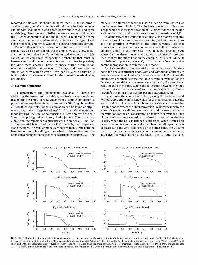
Fig. 1. Effects of omission of appropriate units conversion for the ionic currents on the actleft panels) and a node at the end of the cable (a ventricular node, right panels). Action potlines) and without appropriate units conversion (“Conversion OFF”, dashed lines) for thr(Cm ¼ 1 mF/cm2), the middle panels relate to the case of capacitance reduced by 10%, while

models use different conventions, both differing from Chaste’s, ascan be seen from Table 1. The Purkinje model also illustratesa challenging case for identification of Iion, since it does not includea stimulus current, and has currents given in dimensions of A/F.

To demonstrate the importance of interfacing models properly,six variations of the simulation are presented, half with conversionsand half omitting conversion of the ionic currents. Note thatsimulation time must be units converted (the cellular models usedifferent units) or the numerical method fails. Three differentvalues for the tissue model membrane capacitance Cm are alsoused, to show the effect it has on the coupling. This effect is difficultto distinguish precisely, since Cm also has an effect on actionpotential propagation within the tissue model.

Fig. 1 shows the action potential at two nodes, one a Purkinjenode and one a ventricular node, with and without an appropriateinterface conversion of units for the ionic currents. In Purkinje cellsdifferences are small because the ionic current conversion for thePurkinje cell model involves merely scaling by Cm. For ventricularcells, on the other hand, where the difference between the ioniccurrent units in the model (nA) and the ones expected by Chaste(mA/cm2) is significant, the errors become extremely large.

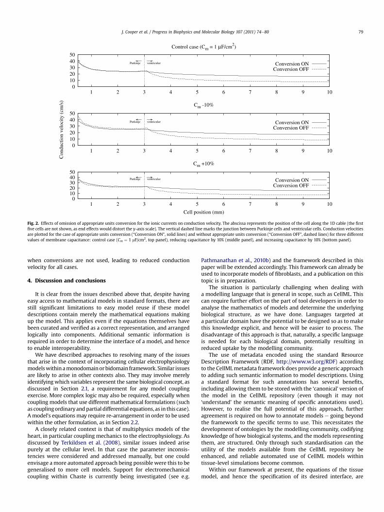
Fig. 2 shows the conduction velocity along the cable with andwithout appropriate units conversion for the ionic currents. Resultsfor three different values of membrane capacitance are shown. ForPurkinje nodes, where the units conversion is a linear scaling by thevalue of capacitance, differences are small and inversely related tothe variations of the cell capacitance, i.e. failing to convert the unitsof the ionic currents caused an underestimation of conductionvelocity when the cell capacitance is increased, while it caused anoverestimation of conduction velocity when the cell capacitance isdecreased. For the ventricular cells, on the other hand, the Iion termis also divided by the model’s value for the membrane capacitance,and since this value (in nF) is less than 1 the Iion term is smaller

-120

-80

-40

0

40

80

0 100 200 300 400 500 600 700 800

Control case (Cm = 1 µF/cm2), ventricular node

Conversion ONConversion OFF

-120

-80

-40

0

40

80

0 100 200 300 400 500 600 700 800

Cm -10%, ventricular node

Conversion ONConversion OFF

-120-80-40

0 40 80

0 100 200 300 400 500 600 700 800

Time (ms)

Cm +10%, ventricular node

ion potential profile at two nodes along the cable: node number 10 (a Purkinje node,entials are plotted for the case of appropriate units conversion (“Conversion ON”, solidee different values of membrane capacitance: the top panels show the control casethe bottom panels correspond to the case of capacitance increased by 10%.

0 10 20 30 40 50

1 2 3 4 5 6 7 8 9 10

Control case (Cm = 1 µF/cm2)

ventricularPurkinje Conversion ONConversion OFF

0 10 20 30 40 50

1 2 3 4 5 6 7 8 9 10

Con

duct

ion

velo

city

(cm

/s)

Cm -10%

ventricularPurkinje Conversion ONConversion OFF

0 10 20 30 40 50

1 2 3 4 5 6 7 8 9 10

Cell position (mm)

Cm +10%

ventricularPurkinje Conversion ONConversion OFF

Fig. 2. Effects of omission of appropriate units conversion for the ionic currents on conduction velocity. The abscissa represents the position of the cell along the 1D cable (the firstfive cells are not shown, as end effects would distort the y-axis scale). The vertical dashed line marks the junction between Purkinje cells and ventricular cells. Conduction velocitiesare plotted for the case of appropriate units conversion (“Conversion ON”, solid lines) and without appropriate units conversion (“Conversion OFF”, dashed lines) for three differentvalues of membrane capacitance: control case (Cm ¼ 1 mF/cm2, top panel), reducing capacitance by 10% (middle panel), and increasing capacitance by 10% (bottom panel).

J. Cooper et al. / Progress in Biophysics and Molecular Biology 107 (2011) 74e80 79

when conversions are not used, leading to reduced conductionvelocity for all cases.

4. Discussion and conclusions

It is clear from the issues described above that, despite havingeasy access to mathematical models in standard formats, there arestill significant limitations to easy model reuse if these modeldescriptions contain merely the mathematical equations makingup the model. This applies even if the equations themselves havebeen curated and verified as a correct representation, and arrangedlogically into components. Additional semantic information isrequired in order to determine the interface of a model, and henceto enable interoperability.

We have described approaches to resolving many of the issuesthat arise in the context of incorporating cellular electrophysiologymodelswithinamonodomainorbidomain framework. Similar issuesare likely to arise in other contexts also. They may involve merelyidentifyingwhich variables represent the same biological concept, asdiscussed in Section 2.1, a requirement for any model couplingexercise. More complex logic may also be required, especially whencoupling models that use different mathematical formulations (suchas couplingordinaryandpartial differential equations, as in this case).A model’s equations may require re-arrangement in order to be usedwithin the other formulation, as in Section 2.2.

A closely related context is that of multiphysics models of theheart, in particular coupling mechanics to the electrophysiology. Asdiscussed by Terkildsen et al. (2008), similar issues indeed arisepurely at the cellular level. In that case the parameter inconsis-tencies were considered and addressed manually, but one couldenvisage amore automated approach being possible were this to begeneralised to more cell models. Support for electromechanicalcoupling within Chaste is currently being investigated (see e.g.

Pathmanathan et al., 2010b) and the framework described in thispaper will be extended accordingly. This framework can already beused to incorporate models of fibroblasts, and a publication on thistopic is in preparation.

The situation is particularly challenging when dealing witha modelling language that is general in scope, such as CellML. Thiscan require further effort on the part of tool developers in order toanalyse the mathematics of models and determine the underlyingbiological structure, as we have done. Languages targeted ata particular domain have the potential to be designed so as to makethis knowledge explicit, and hence will be easier to process. Thedisadvantage of this approach is that, naturally, a specific languageis needed for each biological domain, potentially resulting inreduced uptake by the modelling community.

The use of metadata encoded using the standard ResourceDescription Framework (RDF, http://www.w3.org/RDF) accordingto the CellMLmetadata framework does provide a generic approachto adding such semantic information to model descriptions. Usinga standard format for such annotations has several benefits,including allowing them to be stored with the ‘canonical’ version ofthe model in the CellML repository (even though it may not‘understand’ the semantic meaning of specific annotations used).However, to realise the full potential of this approach, furtheragreement is required on how to annotate models e going beyondthe framework to the specific terms to use. This necessitates thedevelopment of ontologies by the modelling community, codifyingknowledge of how biological systems, and the models representingthem, are structured. Only through such standardisation can theutility of the models available from the CellML repository beenhanced, and reliable automated use of CellML models withintissue-level simulations become common.

Within our framework at present, the equations of the tissuemodel, and hence the specification of its desired interface, are

J. Cooper et al. / Progress in Biophysics and Molecular Biology 107 (2011) 74e8080

hardcoded within the Chaste source code. It would be desirable tohave this portion of the coupled model also available encoded ina markup language, and work on FieldML (Christie et al., 2009) isprogressing in this direction. Interfacing between CellML andFieldML models will require careful consideration of issues such asthose we have discussed.

Finally, while the work described above makes it possible to useany cellular model within a tissue simulation automatically, thisdoes not imply that doing so for a particular scenario is in any waybiologically realistic. A particular cell model may be unsuited to usein a tissue context, or it may have been developed to representparticular experimental conditions, with parameter values andinitial conditions specified accordingly, and give unexpected resultswhen used outside that regime. Further work is thus required ondescribing the scientific questions which the model was developedto address, and hence assisting users in determining its suitabilityfor use in their study. Some initial work on this topic is presented byCooper et al. (2011).

Role of the funding source

JC is partially supported by the European Commission DG-INFSOunder grant numbers 223920 (VPH-NoE) and 224381 (preDiCT). ACwas also partially supported under grant number 224381(preDiCT). The funding bodies had no other role in this work.

Editors’ note

Please see also related communications in this issue by Quinnet al. (2011) and Bradley et al. (2011).

Acknowledgements

The authors would like to thank all other members of the Chastedevelopment team for fruitful discussions on the topics consideredin this manuscript.

References

Beard, D.A., Britten, R., Cooling, M.T., Garny, A., Halstead, M.D.B., Hunter, P.J.,Lawson, J., Lloyd, C.M., Marsh, J., Miller, A., Nickerson, D.P., Nielsen, P.M.F.,Nomura, T., Subramanium, S., Wimalaratne, S.M., Yu, T., 2009. CellML metadatastandards, associated tools and repositories. Physical and Engineering Sciences367, 1845e1867.

Bradley, C., Bowery, A., Britten, R., Budelmann, V., Camara, O., 2011. OpenCMISS:a multi-physics & multi-scale computational infrastructure for the VPH/Physi-ome project. Progress in Biophysics and Molecular Biology, 107, 32e47.

Christie, G.R., Nielsen, P.M.F., Blackett, S.A., Bradley, C.P., Hunter, P.J., 2009. FieldML:concepts and implementation. Philosophical Transactions of the Royal Society A367, 1869e1884.

Clayton, R.H., Bernus, O., Cherry, E.M., Dierckx, H., Fenton, F.H., Mirabella, L.,Panfilov, A.V., Sachse, F.B., Seemann, G., Zhang, H., 2010. Models of cardiac tissueelectrophysiology: progress, challenges and open questions. Progress inBiophysics and Molecular Biology 104, 22e48.

Cooper, J., 2009. Automatic Validation and Optimisation of Biological Models. Ph.D.thesis, University of Oxford.

Cooper, J., McKeever, S., 2008. A model-driven approach to automatic conversion ofphysical units. Software Practice and Experience 38, 337e359.

Cooper, J., Mirams, G., Niederer, S., 2011. High throughput functional curation ofcellular models. Progress in Biophysics and Molecular Biology 107, 11e20.

DiFrancesco, D., Noble, D., 1985. A model of cardiac electrical activity incorporatingionic pumps and concentration changes. Philosophical Transactions of the RoyalSociety B 307, 353e398.

Dokos, S., Celler, B., Lovell, N., 1996. Ion currents underlying sinoatrial node pace-maker activity: a new single cell mathematical model. Journal of TheoreticalBiology 181, 245e272.

Garny, A., Nickerson, D., Cooper, J., dos Santos, R.W., McKeever, S., Nielsen, P.,Hunter, P., 2008. CellML and associated tools and techniques. PhilosophicalTransactions of the Royal Society A 366, 3017e3043.

Hund, T.J., Rudy,Y., 2004.Ratedependenceand regulationofactionpotential andcalciumtransient in a canine cardiac ventricular cell model. Circulation 110, 3168e3174.

Jafri, M.S., Rice, J.J., Winslow, R.L., 1998. Cardiac Ca2þ dynamics: the roles of rya-nodine receptor adaptation and sarcoplasmic reticulum load. BiophysicalJournal 74, 1149e1168.

Keener, J., Sneyd, J., 1998. Mathematical Physiology. In: Interdisciplinary AppliedMathematics, vol. 8. Springer.

Lloyd, C.M., Halstead, M.D., Nielsen, P.F., 2004. CellML: its future, present and past.Progress in Biophysics and Molecular Biology 85, 433e450.

Lloyd, C.M., Lawson, J.R., Hunter, P.J., Nielsen, P.F., 2008. The CellML model reposi-tory. Bioinformatics 24, 2122e2123.

Luo, C., Rudy, Y., 1991. A model of the ventricular cardiac action potential: depolar-ization, repolarization, and their interaction. Circulation Research 68,1501e1526.

Mahajan, A., Shiferaw, Y., Sato, D., Baher, A., Olcese, R., Xie, L.H., Yang, M.J., Chen, P.S.,Restrepo, J.G., Karma, A., Garfinkel, A., Qu, Z., Weiss, J.N., 2008. A rabbitventricular action potential model replicating cardiac dynamics at rapid heartrates. Biophysical Journal 94, 392e410.

Matsuoka, S., Sarai, N., Kuratomi, S., Ono, K., Noma, A., 2003. Role of individual ioniccurrent systems in ventricular cells hypothesized by a model study. The Japa-nese Journal of Physiology 53, 105e123.

Niederer, S.A., Kerfoot, E., Benson, A., Bernabeu, M.O., Bernus, O., Bradley, C., Cherry,E.M., Clayton, R., Fenton, F.H., Garny, A., Heidenreich, E., Land, S., Maleckar, M.,Pathmanathan, P., Plank, G., Rodríguez, J.F., Roy, I., Sachse, F.B., Seemann, G.,Skavhaug, O., Smith, N.P., Verification of cardiac tissue electrophysiologysimulators using an n-version benchmark. Philosophical Transactions of theRoyal Society A, in press.

Noble, D., Varghese, A., Kohl, P., Noble, P., 1998. Improved guinea-pig ventricular cellmodel incorporating a diadic space, iKr

and iKs, length- and tension-dependent

processes. Canadian Journal of Cardiology 14, 123e134.Pathmanathan, P., Bernabeu, M.O., Bordas, R., Cooper, J., Garny, A., Pitt-Francis, J.M.,

Whiteley, J.P., Gavaghan, D.J., 2010a. A numerical guide to the solution of thebidomain equations of cardiac electrophysiology. Progress in Biophysics andMolecular Biology 102, 136e155.

Pathmanathan, P., Chapman, S.J., Gavaghan, D.J., Whiteley, J.P., 2010b. Cardiacelectromechanics: the effect of contraction model on the mathematicalproblem and accuracy of the numerical scheme. The Quarterly Journal ofMechanics and Applied Mathematics 63, 375e399.

Pathmanathan, P., Mirams, G., Southern, J., Whiteley, J., 2011. The significant effect ofthe choice of ionic current integration method in cardiac electro-physiologicalsimulations. International Journal for Numerical Methods in BiomedicalEngineering.

Pitt-Francis, J., Pathmanathan, P., Bernabeu, M.O., Bordas, R., Cooper, J., Fletcher, A.G.,Mirams, G.R., Murray, P., Osbourne, J.M., Walter, A., Chapman, J., Garny, A., vanLeeuwen, I.M.M.,Maini, P.K., Rodriguez, B.,Waters, S.L.,Whiteley, J.P., Byrne, H.M.,Gavaghan, D.J., 2009. Chaste: a test-driven approach to software development forbiological modelling. Computer Physics Communications 180, 2452e2471.

Priebe, L., Beuckelmann, D.J., 1998. Simulation study of cellular electric properties inheart failure. Circulation Research 82, 1206e1223.

Quinn, T., Antzelevitch, C., Bollensdorf, C., Bub, G., RAB, B., Chen, P., 2011. MinimumInformation about a Cardiac Electrophysiology Experiment (MICEE): stand-ardised reporting for model reproducibility, interoperability, and data sharing.Progress in Biophysics and Molecular Biology 107, 4e10.

Sampson, K.J., Iyer, V., Marks, A.R., Kass, R.S., 2010. A computational model ofPurkinje fibre single cell electrophysiology: implications for the long QTsyndrome. The Journal of Physiology 588, 2643e2655.

Stewart, P., Aslanidi, O.V., Noble, D., Noble, P.J., Boyett, M.R., Zhang, H., 2009.Mathematical models of the electrical action potential of Purkinje fibre cells.Philosophical Transactions of the Royal Society A 367, 2225e2255.

Terkildsen, J.R., Niederer, S., Crampin, E.J., Hunter, P., Smith, N.P., 2008. Usingphysiome standards to couple cellular functions for rat cardiac excita-tionecontraction. Experimental Physiology 93, 919e929.

Viswanathan, P.C., Shaw, R.M., Rudy, Y., 1999. Effects of IKr and IKs heterogeneity onaction potential duration and its rate dependence: a simulation study. Circu-lation 99, 2466e2474.