Proc. XII IPRoMM-2016 (Challenges in Manufacturing)
VNIT Nagpur, 22-23 December 2016
2016 IPRoMM-2016
Dynamic analyses of four-bar mechanism in MechAnalyzer software
Rohit Kumar1, Sripad D. Vantmuri2, Rajeevlochana G. Chittawadigi3 and Subir Kumar Saha4
1, 2 Department of Mechanical Engineering, National Institute of Technology Karnataka Surathkal Mangalore, INDIA
3Department of Mechanical Engineering, Amrita School of Engineering, Amrita Vishwa Vidyapeetham
Amrita University, Bengaluru, INDIA
4Department of Mechanical Engineering, Indian Institute of Technology Delhi, New Delhi, INDIA
[email protected], [email protected], [email protected], [email protected]
ABSTRACT
Kinematic and dynamic analyses of mechanisms or machines form a major part in Theory of Machines course. The kinematic analysis involves study of motion of links or parts and is more intuitive to understand. On the other hand, the results of dynamic analysis which deals with forces and moments, are in the form of graph plots and require better understanding of underlying mathematics to comprehend the results. For the effective teaching of kinematics of mechanisms, the authors have developed MechAnalyzer software which has a set of common planar mechanisms that can be selected and analyzed almost instantly. In this paper, the formulation and the implementation of dynamic analysis of four-bar mechanism is presented. A recursive formulation named DeNOC (Decoupled Natural Orthogonal Complement) has been used to perform the inverse and forward dynamics, the results of which have been validated with a commercial software package.
Key words: Planar mechanism, Simulation, Dynamics, Validation, Education
1. INTRODUCTION
A mechanism or a machine consists of various fixed and moving parts or links connected using joints, gears, cams, etc. Based on the application, the dimensions of the links in the form of link length are determined using synthesis of mechanisms or using some standard values and the motion is studied, which form the kinematic analysis. Virtual prototypes of the mechanisms can be developed in a CAD simulation software and the effect of any change in length of the links on the operation of the mechanism can be checked until desired movement is achieved. Hence, software that can be readily used for motion simulation and analysis help in better and effective understanding of the kinematics. Though many commercial software such as ADAMS, RecurDyn, etc. are available for this purpose, their usage in teaching kinematics would require the students to have the knowledge of using those software. Instead, if some of the commonly used mechanisms can be selected, with an option to change the link parameters, the students would be able to learn the concepts more effectively and efficiently. Considering this, MechAnalyzer software was developed by the authors which aims to aid in effective teaching of mechanisms kinematics. Its comparison with other similar software are reported in Hampali et al. (2015) and Rakshith et al. (2015). Another such software is reported by Petuya et al (2014).
Once the motion study or the kinematic analysis is performed, the study of forces in the form of dynamic analysis has to be taken up. The dynamic analysis can be broadly classified as forward and inverse dynamics. The former is the study of the effect of external forces causing the motion of the mechanism, hence useful in the animation of the motion in a simulation environment. On the other hand,

Proc. XII IPRoMM-2016 (Challenges in Manufacturing)
VNIT Nagpur, 22-23 December 2016
2016 IPRoMM-2016
the latter is the determination of the joint forces or torque required to achieve a given motion, which are useful to design the mechanism links so that they are strong enough to perform the required tasks.
The dynamic analysis is performed by deriving the governing equations of motion for the mechanism or the system. Some of the well-known methodologies are Newton-Euler (NE), Euler-Lagrange (EL), Kane’s method, etc. The NE method is based on the vector approach and consists of three translatory equations (Newton’s equations) and three rotational motion equations (Euler’s equations) for each of the link. Further constraint equations are derived for the joints and loop closure. Together, they form a set of Differential Algebraic Equations (DAE). On the contrary, EL method uses energy based approach and the equations of motion of a mechanism can be derived using independent coordinates whose number is equal to the degree-of-freedom (DOF) of the mechanism. The EL methodology results into a set of Ordinary Differential Equations (ODE). Kane’s method also provides ODE that have to solved.
To be implemented in a computer software, the solution methods for ODE are better than those available for solving DAE. Hence, several researchers have proposed formulation of dynamics by beginning with NE approach and later on reducing the number of equations using some constraints or other technique. By doing so, the final set of equations are in the form of ODE and hence can be implemented more easily. A thorough overview on such methods is reported in Chaudhary and Saha (2008). One such method is Decoupled Natural Orthogonal Complement (DeNOC) approach reported by Saha (1999), which was originally proposed for serial chain manipulators or systems.
DeNOC method uses NE equations as a set of block matrices equations for the uncoupled system, where each link is considered to have six DOF and hence free to move around. The constraints are then applied in the form of linear and angular velocities of rigid bodies, and the associated joint rates, after which the minimal set of equations are obtained. There are several advantages of DeNOC over conventional NE or EL formulation, such as: 1) It provides an O(n) algorithm for both inverse and forward dynamics, where n is the number of links in a serial system. 2) All the scalar elements in the matrices and vectors associated with the equations of motion have an analytical expression, which helps in understanding some of the underlying concepts such as articulated body inertia, etc. Also, these help in debugging a computer program. 3) As the methodology is based upon mechanics and linear algebra concepts, it can be understood by under-graduate students. The DeNOC methodology was later extended to closed-loop mechanisms (Chaudhary and Saha, 2008) and tree-type systems (Shah at el. 2012).
In this paper, the formulation for the dynamic analysis of a four-bar mechanism is derived using DeNOC method and discussed in Section 2. The implementation and the usage of software is reported in Section 3 and Section 4 has the validation of results, followed by the conclusions.
2. DYNAMICS OF FOUR-BAR MECHANISM
Four-bar mechanism is one of the important mechanisms that is used to teach the concepts related to kinematics and dynamics. Hence, it was chosen as the first mechanism for the implementation. The inverse dynamics formulation is discussed first, followed by the forward dynamics.
2.1 Inverse Dynamics of Four-bar mechanism
Four-bar mechanism which is a closed loop system, is first divided into an equivalent open
architecture by introducing cuts at appropriate joints. Here, the two subsystems are obtained by
introducing cut-open arrangement at joint J2 as illustrated in Figure 1. The two subsystems obtained
are serial in nature with some constraint existing between them. The cut joints are replaced by
unknown constraint forces, also called Lagrange multipliers. Such subsystem allows one to use
already available well established algorithms for the serial systems. The two subsystem thus
obtained are a one link subsystem, referred as Subsystem I, and a two link subsystem, referred as
Subsystem II. The Lagrange multiplier between these subsystems is represented using 𝜆. The links
are assumed to have their center of masses at a distance of r from one end of the respective links,

Proc. XII IPRoMM-2016 (Challenges in Manufacturing)
VNIT Nagpur, 22-23 December 2016
2016 IPRoMM-2016
such as 𝑟1 for #2 from J1, 𝑟3 for #4 from J4, and 𝑟2 for #3 from J3. The masses of links #2, #3 and #4
are represented by 𝑚2, 𝑚3, and 𝑚4, respectively. To derive the equations of motion for the closed
loop system, two subsystems and have been considered, i.e. one body in Subsystem I and two bodies
in Subsystem II and the subsystems are represented using superscripts of I and II, respectively. The
steps followed in the inverse dynamics analysis are explained next.
a. Uncoupled Newton-Euler Equations of motion
Referring to Figure 2, consider 𝑖𝑡ℎ link with 𝑚𝑖 as mass of the link whose center of mass (𝐶𝑖) is located by vector 𝐜𝑖 in a fixed frame of reference. External force 𝐟𝑖 and moment 𝐧𝑖 are acting on the link causing its motion.
The NE equations of motion for the 𝑖𝑡ℎ link can be derived using free body diagram as
𝐟𝑖 = 𝑚𝑖�̈�𝑖 (1) 𝐧𝑖 = 𝐈𝑖�̇�𝑖 + 𝛚𝑖 × 𝐈𝑖𝛚𝑖 (2)
Equations (1) and (2) can be written in a compact form using matrices and vectors as
𝐌𝑖 �̇�𝑖 + 𝐖𝑖𝐌𝑖𝐭𝑖 = 𝐰𝑖 (3)
where 𝐌𝑖 and 𝐖𝑖 are 6 × 6 mass inertia matrix, and the matrix of angular velocities respectively and are given by
𝐌𝑖 ≡ [𝐈𝑖 𝟎𝟎 𝑚𝑖𝟏
]; and 𝐖𝑖 ≡ [𝛚𝑖 × 𝟏 𝟎
𝟎 𝟎] (4)
where 𝐈𝑖 denotes the 3 × 3 inertia tensor of the body and 𝛚𝑖 × 𝟏 is 3 × 3 cross product tensor associated with angular velocity. Also, 1 and 0 are the 3 × 3 identity and zero matrices respectively. Furthermore, the 6-dimensional twist vector 𝐭𝑖 , and wrench vector 𝐰𝑖 are defined as
Figure 2: External force and moment acting on a rigid body or link
Figure 1: Four-bar mechanism converted into two serial subsystems
−𝝀
𝝀
𝜃2 𝜃4
𝜃3
Subsystem I Subsystem II
Input torque: 𝝉𝟏
#2
#1
#3
#4
𝑟1
𝑑1
𝑑2
𝑟2
𝑑3
𝑟3

Proc. XII IPRoMM-2016 (Challenges in Manufacturing)
VNIT Nagpur, 22-23 December 2016
2016 IPRoMM-2016
𝐭𝑖 ≡ [𝛚𝑖
�̇�𝑖] and 𝐰𝑖 ≡ [
𝐧𝑖
𝐟𝑖] (5)
The NE equations of the uncoupled system with n moving bodies can be combined into a single block matrix equation as
𝐌�̇� + 𝐖𝐌𝐭 = 𝐰 (6)
where 𝐌 and 𝐖 are 6𝑛 × 6𝑛 generalized mass inertia matrix, and the generalized matrix of angular velocities, respectively. For the four-bar mechanism in Figure 1, the NE equations for the uncoupled subsystems I and II are written as
𝐌𝐼 ≡ 𝐌1 and 𝐖𝐼 ≡ 𝐖1
𝐭𝐼 ≡ 𝐭𝟏 and 𝐰𝐼 ≡ 𝐰𝟏 (7)
𝐌𝐼𝐼 ≡ 𝑑𝑖𝑎𝑔. [𝐌4, 𝐌3] and 𝐖𝐼𝐼 ≡ 𝑑𝑖𝑎𝑔. [𝐖4, 𝐖3]
𝐭𝐼𝐼 ≡ [𝐭4𝑇 , 𝐭3
𝑇]𝑇 and 𝐰𝐼𝐼 ≡ [𝐰4𝑇 , 𝐰3
𝑇]𝑇 (8)
b. Kinematic constraints:
For a serial system represented using Equation (6), kinematic constraints in the velocity level are applied to get a system of ODE in the minimal form. Velocity level constraints are obtained as a function of the joint rates as
𝐭 = 𝐍�̇� (9)
where N is a 6𝑛 × 𝑛 matrix, known as Natural Orthogonal Complement (Angeles and Ma, 1988), whose utility is explained in the next sub-section. In the DeNOC method, N is further decoupled into two matrices as
𝐍 ≡ 𝐍𝐥𝐍𝐝 (10)
where 𝐍𝑙 is a 6𝑛 × 𝑛 lower diagonal matrix and 𝐍𝑑 is an n dimensional diagonal matrix. These matrices allow one to develop recursive inverse and forward dynamics algorithms that are required in control and simulation of various robotic systems. For the four-bar mechanism considered here, the links in Subsystem II are coupled by revolute joints. The angular and linear velocity of #3 can be derived from link #4. The kinematic constraint can be written in following form:
𝛚3 = 𝛚4 + 𝐞3�̇�3 (11)
�̇�3 = �̇�4 + 𝛚4 × 𝐫3 + 𝛚3 × 𝐝2 (12)
where 𝐞3 ≡ [0 0 1]𝑇 ,i.e. the axis of the revolute joint which is along the Z axis. The compact form of the twist vector of Subsystem II can be written as
𝐭𝑰𝑰 = 𝐍𝑰𝑰�̇�𝑰𝑰 where 𝐍𝑰𝑰 ≡ 𝐍𝑙𝐼𝐼𝐍𝑑
𝐼𝐼 (13)
The DeNOC matrices for Subsystem II is obtained as below
Proc. XII IPRoMM-2016 (Challenges in Manufacturing)
VNIT Nagpur, 22-23 December 2016
2016 IPRoMM-2016
𝐍𝑙𝐼𝐼 ≡ [
𝟏 0𝐁21 𝟏
] ; 𝐍𝑑𝐼𝐼 ≡ [
𝐩1𝐼𝐼 0
0 𝐩2𝐼𝐼] ; and �̇�𝐼𝐼 ≡ [
�̇�4
�̇�3
]
where 𝐁21 ≡ [𝟏 𝟎
−(𝐫2 + 𝐝3) × 𝟏 𝟏] and 𝐩𝑖 ≡ [𝐞𝑖 𝐞𝑖 × 𝐝𝑖]
𝑇
(14)
Similarly for Subsystem I, which just has a single link with a revolute joint, the constraints equations are
𝐍𝑙𝐼 ≡ [𝟏] ; 𝐍𝑑
𝐼 ≡ [𝐩1𝐼 ] ; and �̇�𝐼 ≡ [�̇�2] (15)
c. Coupled Equations of Motion
The uncoupled NE equations of motion of Equation (9) are pre-multiplied by 𝐍𝑇 on both sides. The constraints equations are orthogonal to the twist vector t and hence are eliminated from the overall equations. Hence uncoupled equations (NE) are converted into minimal set of equations.
𝐍𝑇(𝐌�̇� + 𝐖𝐌𝐭) = 𝐍𝑇𝐰 (16)
By using �̇� = 𝐍�̈� + �̇��̇�, Equation (16) can be written in block matrices and vectors form as
𝐈�̈� + 𝐂�̇� = 𝛕 + 𝛕𝑔 (17)
where 𝛕𝑔 is the gravity vector and 𝛕 is the torques at the joints and the other terms are
𝐈 ≡ 𝐍𝑇𝐌𝐍 ; 𝐂 ≡ 𝐍𝑇(𝐌�̇� + 𝐖𝐌𝐍) ; and 𝛕 = 𝐍𝑇𝐰 (18)
For Subsystem II, the input torques are zero, i.e., the torques at the joints J4 and J3 are zero. The unknown constraint forces or Lagrange multiplier 𝛌, a 3 × 1 vector is calculated using
𝐈𝐼𝐼�̈�𝐼𝐼 + 𝐂𝐼𝐼�̇�𝐼𝐼 = 𝛕𝑔 + (𝐉𝐼𝐼)𝑇(−𝛌) (19)
Vector 𝛌 from Equation (19) is substituted in Subsystem I to get the input torque as
𝐼𝐼�̈�𝐼 + 𝐶𝐼�̇�𝐼 = 𝜏1 + 𝜏𝑔 + (𝐉𝐼)𝑇(𝛌) (20)
where 𝐉𝐼 = [−𝑙2 sin(𝜃2)
𝑙2cos (𝜃2)] and 𝐉𝐼𝐼 = [
−𝑙4 sin(𝜃4) − 𝑙3 sin(𝜃3 + 𝜃4)
𝑙4cos (θ4) + 𝑙3 cos(𝜃3 + 𝜃4) 𝑙3sin (𝜃3 + 𝜃4) 𝑙3cos (𝜃3 + 𝜃4)
] are Jacobian
matrices for subsystem I and II, respectively and 𝑙2, 𝑙3 and 𝑙4 are lengths of links #2, #3 and #4 respectively. These Jacobian matrices relate the linear velocity of the links with the angular velocities of the joints. Using Equation (20), the input torque at joint J1 (𝜏1) is determined, thus completing the inverse dynamic analysis.
2.2 Forward Dynamics of Four-bar mechanism The forward dynamics is done by knowing the kinematic and inertial parameters and joint torques and forces to find the trajectories of the joints of a mechanism. For known input and external
forces/torques, vector 𝛉. The vector 𝛉 for a given torque 𝛕 is found out by calculating �̈� and then integrating to find velocity and position. The two subsystems obtained above for the four-bar mechanism are rewritten to obtain the position and velocity by calculating accelerations. The constrained equations of motion obtained in Equations (19) and (20) are combined with velocity constraints Equation (21) to obtain differential algebraic equations(DAE) as

Proc. XII IPRoMM-2016 (Challenges in Manufacturing)
VNIT Nagpur, 22-23 December 2016
2016 IPRoMM-2016
[𝐉𝐼 −𝐉𝐼𝐼] [ �̇�𝐼
�̇�𝐼𝐼] = [
0𝟎
] (21)
[
𝐼𝐼 𝟎 (𝐉𝐼)𝑇
0 𝐈𝐼𝐼 −(𝐉𝐼𝐼)𝑇
𝐉𝐼 −𝐉𝐼𝐼 𝟎
] [�̈�𝐼
�̈�𝐼𝐼
𝛌
] ≡ [
𝜏1 + 𝜏𝑔 − 𝐶𝐼�̇�𝐼
𝛕𝑔 − 𝐂𝐼𝐼�̇�𝐼𝐼
−�̇�𝐼�̇�𝐼 + �̇�𝐼𝐼�̇�𝐼𝐼
] (22)
Let A denote the matrix on LHS, x be the vector containing accelerations terms and Lagrange multiplier, and B be the matrix on the RHS. Hence x can be found out by following equation.
𝐱 = 𝐀−1𝐁 (23)
Here, since matrix A is symmetric positive definite, it is always invertible. As the DAE obtained are highly non-linear and cannot be solved analytically, a suitable numerical technique has to be used to determine the joint accelerations, thus completing the forward dynamics analysis. The numerical technique used for forward dynamic analysis is Runge-Kutta method. The initial conditions considered for the analyses is taken to be at rest, making initial velocities and accelerations of all the links as zero. The initial position for link #2 is at rest while #3 and #4 is found by position analysis through vector closed loop equations. These initial conditions are used to calculate the accelerations and then integrated using Runge-Kutta method to find the velocity and position consecutively, which are then used for finding the new acceleration. The iterative procedure is continued till the given number of steps and time as input by the user.
3. IMPLEMENTATION IN MECHANALYZER
The kinematic analysis of a four-bar mechanism was already existing in MechAnalyzer Version 4 (Lokesh et al, 2015). Version 5 has dynamics of a four-bar mechanism implemented, in addition to some other additional features and modules. User can easily change the length of the links and the 3D model of the mechanism gets updated instantly. The mass and inertia properties of the links can be changed to perform the dynamic analysis. The software has been developed using Visual C# programming language and the formulations of inverse and forward dynamics discussed in the previous section are implemented. A screenshot of MechAnalyzer software is shown in Figure 3.
Figure 3: Graphical User Interface (GUI) of MechAnalyzer showing a four-bar mechanism
3D model of mechanism
Mass and inertia
properties
Toggle window for graph plots
Proc. XII IPRoMM-2016 (Challenges in Manufacturing)
VNIT Nagpur, 22-23 December 2016
2016 IPRoMM-2016
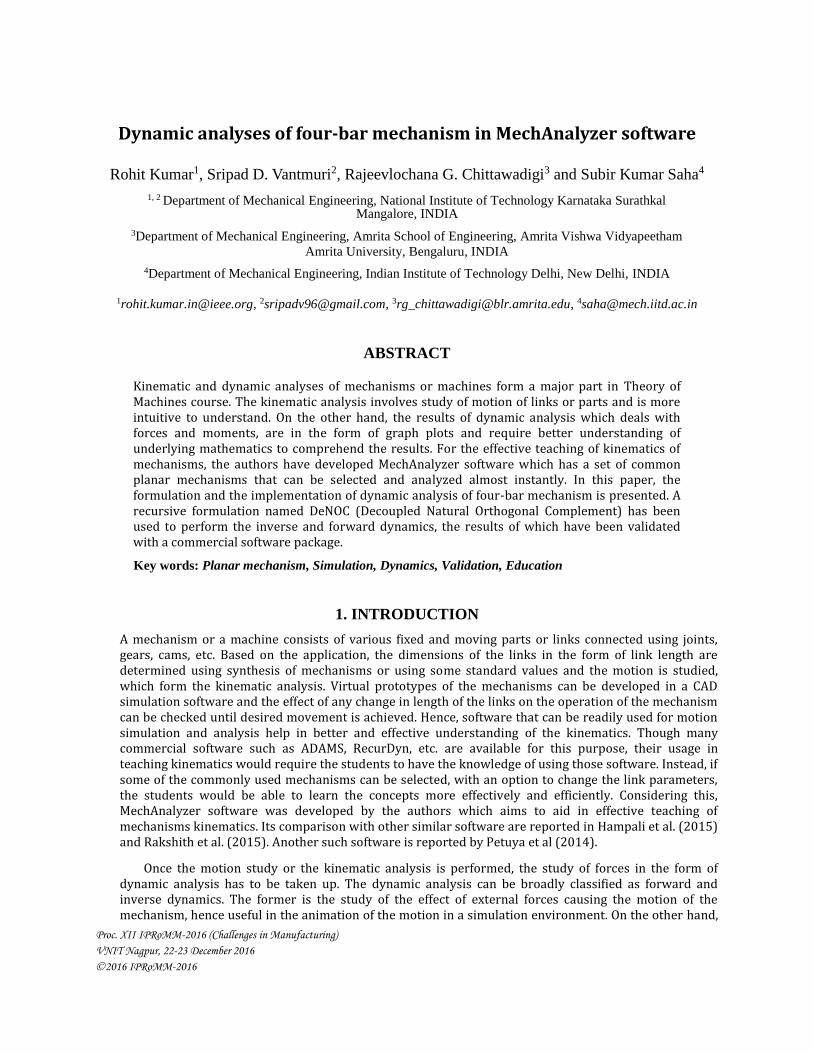
For the set values of mass and inertia properties, and the input joint trajectory, the driving torque for joint J1 is determined as a part of inverse dynamics. The results obtained can be easily viewed as graph plots in the software. The graph plots are developed using ZedGraph, an open source library for plots. For the mechanism shown in Figure 3, the input joint torque determined with and without gravity, are shown in Figures 4(a) and 4(b), respectively. Similarly, for the forward dynamics, the motion of the mechanism due to the action of gravity can be seen. The plots of the joint angle, velocity and acceleration can also be plotted.
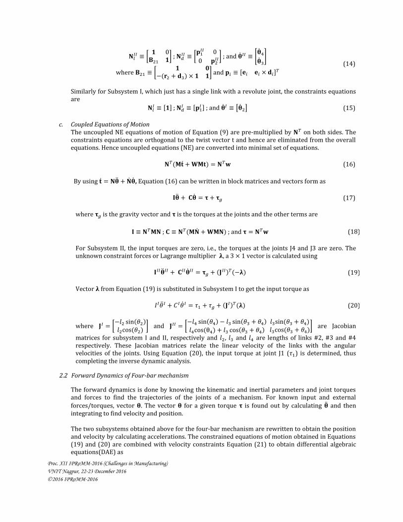
Though plots of dynamic analysis are useful in design and simulation of mechanisms, they are not as intuitive as kinematic analysis results for students to understand and comprehend. However, using MechAnalyzer software, the effect of change of mass and inertia properties of links on the torque can be illustrated by comparing different plots. For example, for different values of mass of coupler link (link #3), the driving torque obtained through inverse dynamics is plotted as shown in Figure 5. It can be noted that for higher mass, more torque is required to rotate the crank link, hence making students understand an underlying concept.
4. VALIDATION OF RESULTS
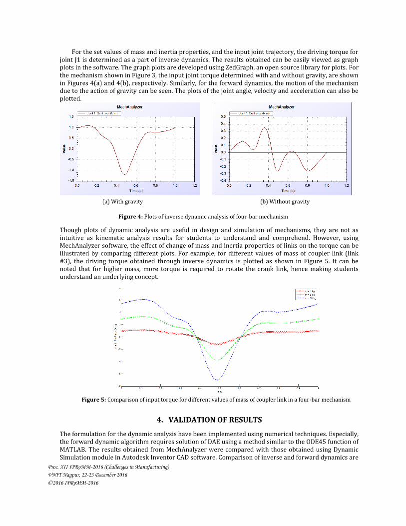
The formulation for the dynamic analysis have been implemented using numerical techniques. Especially, the forward dynamic algorithm requires solution of DAE using a method similar to the ODE45 function of MATLAB. The results obtained from MechAnalyzer were compared with those obtained using Dynamic Simulation module in Autodesk Inventor CAD software. Comparison of inverse and forward dynamics are
Figure 5: Comparison of input torque for different values of mass of coupler link in a four-bar mechanism
(a) With gravity
Figure 4: Plots of inverse dynamic analysis of four-bar mechanism
(b) Without gravity
Proc. XII IPRoMM-2016 (Challenges in Manufacturing)
VNIT Nagpur, 22-23 December 2016
2016 IPRoMM-2016
shown in Figures 6(a) and 6(b), respectively. The plots matched exactly, thus validating the formulation and implementation of the dynamics algorithm in MechAnalyzer software.
5. CONCLUSION
The formulation and the implementation details of the dynamic analysis of four-bar mechanism in MechAnalyzer software have been presented in this paper. The formulation used is based on DeNOC methodology which is a recursive algorithm. The output of the analyses can be viewed as animation and also in the form of graph plots, which would help in effective teaching and learning of the concepts related to dynamics. As four-bar mechanism is commonly used in teaching, it has been implemented first. In the future, dynamic analyses of more such mechanisms will be implemented in MechAnalyzer. The reported implementation is available in MechAnalyzer Version 5, which can be downloaded for free from http://www.roboanalyzer.com/mechanalyzer.html.
6. REFERENCES
[1] Angeles, J.; Ma, O.: Dynamic Simulation of n-axis Serial Robotic Manipulators using a Natural Orthogonal
Complement. The International Journal of Robotics Research. Vol. 7, No. 5, pp. 32-47, 1988.
[2] Chaudhary, H.; Saha, S. K. Dynamics and Balancing of Multibody Systems, Springer, 2008.
[3] Hampali, S.; Chittawadigi, R. G.; Saha, S. K.: MechAnalyzer: A 3D Model Based Mechanism Learning
Software. In P. 14th World Congress in Mechanism and Machine Science, 2015.
[4] Lokesh, R.; Chittawadigi, R. G.; Saha, S. K.: MechAnalyzer: 3D Simulation Software to Teach Kinematics of
Machines. In P. 2nd International and 17th National Conference on Machines and Mechanisms, 2015.
[5] Petuya, V.; Macho, E.; Altuzarra, O.; Pinto C.; Hernandez, A.: Educational software tools for the kinematic
analysis of mechanisms. Computer Applications in Engineering Education. Vol. 22, No. 1, pp. 72-86, 2014.
[6] Saha, S. K.: Dynamics of serial multibody systems using the decoupled natural orthogonal complement
matrices, Journal of Applied Mechanics, 1999.
[7] Shah, S. V.; Saha, S. K.; Dutt, J. K. Dynamics of Tree-type Robotics Systems, Springer, 2013.
(a) Inverse dynamics without gravity (b) Angular velocity of joint 3 for forward dynamics
Figure 6: Validation of results with Dynamic Simulation module of Autodesk Inventor software
Recommended


![Bar Briefs · James Maceroni [2016] (586) 465-4900 Peter W. Peacock [2016 ... In mediations, ... you can now see archived Bar . Bar Briefs • November 2014. Bar Briefs](https://img.pdfslide.net/doc/110x75/5b550d287f8b9a0d398dc8ea/bar-briefs-james-maceroni-2016-586-465-4900-peter-w-peacock-2016-in.jpg)