Hypothesis Testing, Power, Sample Size and Confidence Intervals (Part 1)
Hypothesis Testing, Power, Sample Size andConfidence Intervals (Part 1)
B.H. Robbins Scholars Series
June 3, 2010
1 / 44
Hypothesis Testing, Power, Sample Size and Confidence Intervals (Part 1)
OutlineIntroduction to hypothesis testing
Scientific and statistical hypothesesClassical and Bayesian paradigmsType 1 and type 2 errors
One sample test for the meanHypothesis testingPower and sample sizeConfidence interval for the meanSpecial case: paired data
One sample methods for a probabilityHypothesis testingPower, confidence intervals, and sample size
Two sample tests for meansHypothesis testsPower, confidence intervals, and sample size
2 / 44
Hypothesis Testing, Power, Sample Size and Confidence Intervals (Part 1)
Introduction to hypothesis testing
Introduction
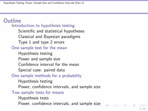
I Goal of hypothesis testing is to rule out chance as anexplanation for an observed effect
I Example: Cholesterol lowering medicationsI 25 people treated with a statin and 25 with a placeboI Average cholesterol after treatment is 180 with statins and 200
with placebo.
I Do we have sufficient evidence to suggest that statins lowercholesterol?
I Can we be sure that statin use as opposed to a chanceoccurrence led to lower cholesterol levels?
3 / 44
Hypothesis Testing, Power, Sample Size and Confidence Intervals (Part 1)
Introduction to hypothesis testing
Scientific and statistical hypotheses
Hypotheses
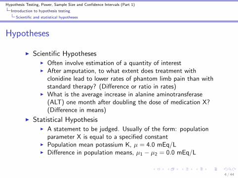
I Scientific HypothesesI Often involve estimation of a quantity of interestI After amputation, to what extent does treatment with
clonidine lead to lower rates of phantom limb pain than withstandard therapy? (Difference or ratio in rates)
I What is the average increase in alanine aminotransferase(ALT) one month after doubling the dose of medication X?(Difference in means)
I Statistical HypothesisI A statement to be judged. Usually of the form: population
parameter X is equal to a specified constantI Population mean potassium K, µ = 4.0 mEq/LI Difference in population means, µ1 − µ2 = 0.0 mEq/L
4 / 44
Hypothesis Testing, Power, Sample Size and Confidence Intervals (Part 1)
Introduction to hypothesis testing
Scientific and statistical hypotheses
Statistical Hypotheses
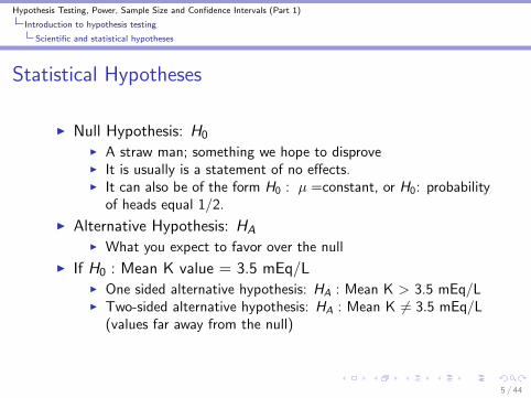
I Null Hypothesis: H0
I A straw man; something we hope to disproveI It is usually is a statement of no effects.I It can also be of the form H0 : µ =constant, or H0: probability
of heads equal 1/2.
I Alternative Hypothesis: HA
I What you expect to favor over the null
I If H0 : Mean K value = 3.5 mEq/LI One sided alternative hypothesis: HA : Mean K > 3.5 mEq/LI Two-sided alternative hypothesis: HA : Mean K 6= 3.5 mEq/L
(values far away from the null)
5 / 44
Hypothesis Testing, Power, Sample Size and Confidence Intervals (Part 1)
Introduction to hypothesis testing
Classical and Bayesian paradigms
Classical (Frequentist) Statistics
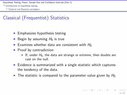
I Emphasizes hypothesis testing
I Begin by assuming H0 is true
I Examines whether data are consistent with H0
I Proof by contradictionI If, under H0, the data are strange or extreme, then doubts are
cast on the null.
I Evidence is summarized with a single statistic which capturesthe tendency of the data.
I The statistic is compared to the parameter value given by H0
6 / 44
Hypothesis Testing, Power, Sample Size and Confidence Intervals (Part 1)
Introduction to hypothesis testing
Classical and Bayesian paradigms
Classical (Frequentist) Statistics
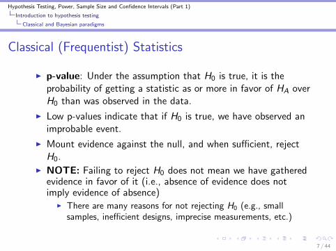
I p-value: Under the assumption that H0 is true, it is theprobability of getting a statistic as or more in favor of HA overH0 than was observed in the data.
I Low p-values indicate that if H0 is true, we have observed animprobable event.
I Mount evidence against the null, and when sufficient, rejectH0.
I NOTE: Failing to reject H0 does not mean we have gatheredevidence in favor of it (i.e., absence of evidence does notimply evidence of absence)
I There are many reasons for not rejecting H0 (e.g., smallsamples, inefficient designs, imprecise measurements, etc.)
7 / 44
Hypothesis Testing, Power, Sample Size and Confidence Intervals (Part 1)
Introduction to hypothesis testing
Classical and Bayesian paradigms
Classical (Frequentist) Statistics
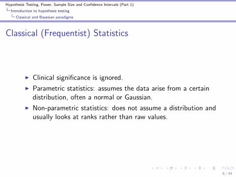
I Clinical significance is ignored.
I Parametric statistics: assumes the data arise from a certaindistribution, often a normal or Gaussian.
I Non-parametric statistics: does not assume a distribution andusually looks at ranks rather than raw values.
8 / 44
Hypothesis Testing, Power, Sample Size and Confidence Intervals (Part 1)
Introduction to hypothesis testing
Classical and Bayesian paradigms
Bayesian Statistics
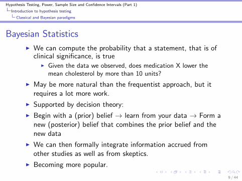
I We can compute the probability that a statement, that is ofclinical significance, is true
I Given the data we observed, does medication X lower themean cholesterol by more than 10 units?
I May be more natural than the frequentist approach, but itrequires a lot more work.
I Supported by decision theory:
I Begin with a (prior) belief → learn from your data → Form anew (posterior) belief that combines the prior belief and thenew data
I We can then formally integrate information accrued fromother studies as well as from skeptics.
I Becoming more popular.
9 / 44
Hypothesis Testing, Power, Sample Size and Confidence Intervals (Part 1)
Introduction to hypothesis testing
Type 1 and type 2 errors
Errors in Hypothesis Testing
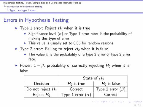
I Type 1 error: Reject H0 when it is trueI Significance level (α) or Type 1 error rate: is the probability of
making this type of errorI This value is usually set to 0.05 for random reasons
I Type 2 error: Failing to reject H0 when it is falseI The value β is the probability of a type 2 error or type 2 error
rate.
I Power: 1− β: probability of correctly rejecting H0 when it isfalse
State of H0
Decision H0 is true H0 is false
Do not reject H0 Correct Type 2 error (β)
Reject H0 Type 1 error (α) Correct
10 / 44
Hypothesis Testing, Power, Sample Size and Confidence Intervals (Part 1)
Introduction to hypothesis testing
Type 1 and type 2 errors
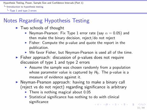
Notes Regarding Hypothesis TestingI Two schools of thought
I Neyman-Pearson: Fix Type 1 error rate (say α = 0.05) andthen make the binary decision, reject/do not reject
I Fisher: Compute the p-value and quote the report in thepublication.
I We favor Fisher, but Neyman-Pearson is used all of the time.I Fisher approach: discussion of p-values does not require
discussion of type 1 and type 2 errorsI Assume the sample was chosen randomly from a population
whose parameter value is captured by H0. The p-value is ameasure of evidence against it.
I Neyman-Pearson approach: having to make a binary call(reject vs do not reject) regarding significance is arbitrary
I There is nothing magical about 0.05I Statistical significance has nothing to do with clinical
significance
11 / 44
Hypothesis Testing, Power, Sample Size and Confidence Intervals (Part 1)
One sample test for the mean
Hypothesis testing
One sample test for the mean
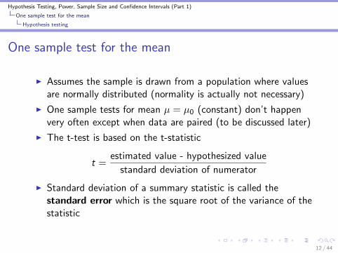
I Assumes the sample is drawn from a population where valuesare normally distributed (normality is actually not necessary)
I One sample tests for mean µ = µ0 (constant) don’t happenvery often except when data are paired (to be discussed later)
I The t-test is based on the t-statistic
t =estimated value - hypothesized value
standard deviation of numerator
I Standard deviation of a summary statistic is called thestandard error which is the square root of the variance of thestatistic
12 / 44
Hypothesis Testing, Power, Sample Size and Confidence Intervals (Part 1)
One sample test for the mean
Hypothesis testing
One sample test for the mean
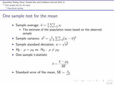
I Sample average: x = 1n
∑ni=1 xi
I The estimate of the population mean based on the observedsample
I Sample variance: s2 = 1n−1
∑ni=1(xi − x)2
I Sample standard deviation: s =√s2
I H0 : µ = µ0 vs. HA : µ 6= µ0
I One sample t-statistic
t =x − µ0
SE
I Standard error of the mean, SE = s√n
13 / 44
Hypothesis Testing, Power, Sample Size and Confidence Intervals (Part 1)
One sample test for the mean
Hypothesis testing
One sample t-test for the mean
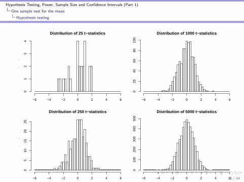
I When data come from a normal distribution and H0 holds, thet ratio follows the t− distribution. What does that mean?
I Draw a sample from the population, conduct the study andcalculate the t-statistic.
I Do it again, and calculate the t-statistic again.
I Do it again and again.
I Now look at the distribution of all of those t-statistics.
I This tells us the relative probabilities of all t-statistics if H0 istrue.
14 / 44
Hypothesis Testing, Power, Sample Size and Confidence Intervals (Part 1)
One sample test for the mean
Hypothesis testing
Example: one sample t-test for the mean
I The distribution of potassium concentrations in the targetpopulation are normally distributed with mean 4.3 andvariance .1: N(4.3, .1).
I H0 : µ = 4.3 vs. HA : µ 6= 4.3. Note that H0 is true!I Each time the study is done,
I Sample 100 participantsI Calculate:
t =x − 4.3
SE
I Conduct the study 25 times, 250 times, 1000 times, 5000times
15 / 44
Hypothesis Testing, Power, Sample Size and Confidence Intervals (Part 1)
One sample test for the mean
Hypothesis testing
Distribution of 25 t−statistics
t−values
Fre
quen
cy
−6 −4 −2 0 2 4 6
01
23
4
Distribution of 250 t−statistics
Fre
quen
cy
−6 −4 −2 0 2 4 6
05
1015
2025
Distribution of 1000 t−statistics
t−values
Fre
quen
cy
−6 −4 −2 0 2 4 6
020
4060
8010
0
Distribution of 5000 t−statistics
Fre
quen
cy
−6 −4 −2 0 2 4 6
010
020
030
040
050
0
16 / 44
Hypothesis Testing, Power, Sample Size and Confidence Intervals (Part 1)
One sample test for the mean
Hypothesis testing
One sample t-test for the mean
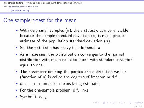
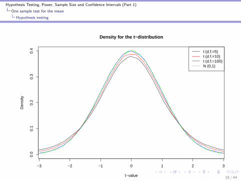
I With very small samples (n), the t statistic can be unstablebecause the sample standard deviation (s) is not a preciseestimate of the population standard deviation (σ).
I So, the t-statistic has heavy tails for small n
I As n increases, the t-distribution converges to the normaldistribution with mean equal to 0 and with standard deviationequal to one.
I The parameter defining the particular t-distribution we use(function of n) is called the degrees of freedom or d.f.
I d.f. = n - number of means being estimated
I For the one-sample problem, d.f.=n-1
I Symbol is tn−1
17 / 44
Hypothesis Testing, Power, Sample Size and Confidence Intervals (Part 1)
One sample test for the mean
Hypothesis testing
−3 −2 −1 0 1 2 3
0.0
0.1
0.2
0.3
0.4
Density for the t−distribution
t−value
Den
sity
t (d.f.=5)t (d.f.=10)t (d.f.=100)N (0,1)
18 / 44
Hypothesis Testing, Power, Sample Size and Confidence Intervals (Part 1)
One sample test for the mean
Hypothesis testing
One sample t-test for the mean
I One sided test: H0 : µ = µ0 versus HA : µ > µ0
I One tailed p-value:I Probability of getting a value from the tn−1 distribution that is
at least as much in favor of HA over H0 than what we hadobserved.
I Two-sided test: H0 : µ = µ0 versus HA : µ 6= µ0
I Two-tailed p-value:I Probability of getting a value from the tn−1 distribution that is
at least as big in absolute value as the one we observed.
19 / 44
Hypothesis Testing, Power, Sample Size and Confidence Intervals (Part 1)
One sample test for the mean
Hypothesis testing
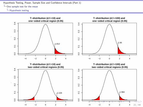
One sample t-test for the mean
I Computer programs can compute the p-value for a given nand t-statistic
I Critical valueI The value in the t (or any other) distribution that, if exceeded,
yields a ’statistically significant’ result for type 1 error rateequal to α
I Critical regionI The set of all values that are considered statistically
significantly different from H0.
20 / 44
Hypothesis Testing, Power, Sample Size and Confidence Intervals (Part 1)
One sample test for the mean
Hypothesis testing
−4 −2 0 2 4
0.0
0.1
0.2
0.3
0.4
T−distribution (d.f.=10) and one−sided critical region (0.05)
t−value
dens
ity
1.812
−4 −2 0 2 4
0.0
0.1
0.2
0.3
0.4
T−distribution (d.f.=10) and two−sided critical regions (0.05)
dens
ity
2.228
−4 −2 0 2 4
0.0
0.1
0.2
0.3
0.4
T−distribution (d.f.=100) and one−sided critical region (0.05)
t−value
dens
ity
1.66
−4 −2 0 2 4
0.0
0.1
0.2
0.3
0.4
T−distribution (d.f.=100) and two−sided critical regions (0.05)
dens
ity
1.984
21 / 44
Hypothesis Testing, Power, Sample Size and Confidence Intervals (Part 1)
One sample test for the mean
Power and sample size
Power and Sample Size for a one sample test of means
I Power increases whenI Type 1 error rate (α) increases: type 1 (α) versus type 2 (β)
tradeoffI True µ is very far from µ0
I Variance or standard deviation (σ) decreases (decrease noise)I Sample size increases
I T-statistic
t =x − µ0
σ/√n
I Power for a 2-tailed test is a function of the true mean µ, thehypothesized mean µ0, and the standard deviation σ onlythrough |µ− µ0|/σ
22 / 44
Hypothesis Testing, Power, Sample Size and Confidence Intervals (Part 1)
One sample test for the mean
Power and sample size
Power and Sample Size for a one sample test of means
I Sample size to achieve α = 0.05, power=0.90 is approximately
n = 10.51
(σ
µ− µ0
)2
I Power calculators can be found at statpages.org/#Power
I PS is a very good power calculator (Dupont and Plummer):http://biostat.mc.vanderbilt.edu/PowerSampleSize
23 / 44
Hypothesis Testing, Power, Sample Size and Confidence Intervals (Part 1)
One sample test for the mean
Power and sample size
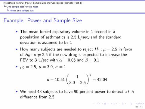
Example: Power and Sample Size
I The mean forced expiratory volume in 1 second in apopulation of asthmatics is 2.5 L/sec, and the standarddeviation is assumed to be 1
I How many subjects are needed to reject H0 : µ = 2.5 in favorof H0 : µ 6= 2.5 if the new drug is expected to increase theFEV to 3 L/sec with α = 0.05 and β = 0.1
I µ0 = 2.5, µ = 3.0, σ = 1
n = 10.51
(1
3.0− 2.5
)2
= 42.04
I We need 43 subjects to have 90 percent power to detect a 0.5difference from 2.5.
24 / 44
Hypothesis Testing, Power, Sample Size and Confidence Intervals (Part 1)
One sample test for the mean
Confidence interval for the mean
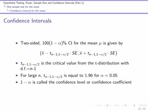
Confidence Intervals
I Two-sided, 100(1− α)% CI for the mean µ is given by
(x − tn−1,1−α/2 · SE , x + tn−1,1−α/2 · SE )
I tn−1,1−α/2 is the critical value from the t-distribution withd.f.=n-1
I For large n, tn−1,1−α/2 is equal to 1.96 for α = 0.05
I 1− α is called the confidence level or confidence coefficient
25 / 44
Hypothesis Testing, Power, Sample Size and Confidence Intervals (Part 1)
One sample test for the mean
Confidence interval for the mean
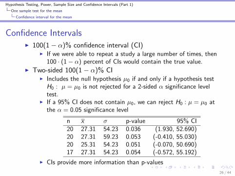
Confidence IntervalsI 100(1− α)% confidence interval (CI)
I If we were able to repeat a study a large number of times, then100 · (1− α) percent of CIs would contain the true value.
I Two-sided 100(1− α)% CII Includes the null hypothesis µ0 if and only if a hypothesis test
H0 : µ = µ0 is not rejected for a 2-sided α significance leveltest.
I If a 95% CI does not contain µ0, we can reject H0 : µ = µ0 atthe α = 0.05 significance level
n x σ p-value 95% CI20 27.31 54.23 0.036 (1.930, 52.690)20 27.31 59.23 0.053 (-0.410, 55.030)20 25.31 54.23 0.051 (-0.070, 50.690)17 27.31 54.23 0.054 (-0.572, 55.192)
I CIs provide more information than p-values
26 / 44
Hypothesis Testing, Power, Sample Size and Confidence Intervals (Part 1)
One sample test for the mean
Special case: paired data
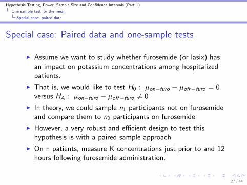
Special case: Paired data and one-sample tests
I Assume we want to study whether furosemide (or lasix) hasan impact on potassium concentrations among hospitalizedpatients.
I That is, we would like to test H0 : µon−furo − µoff−furo = 0versus HA : µon−furo − µoff−furo 6= 0
I In theory, we could sample n1 participants not on furosemideand compare them to n2 participants on furosemide
I However, a very robust and efficient design to test thishypothesis is with a paired sample approach
I On n patients, measure K concentrations just prior to and 12hours following furosemide administration.
27 / 44
Hypothesis Testing, Power, Sample Size and Confidence Intervals (Part 1)
One sample test for the mean
Special case: paired data
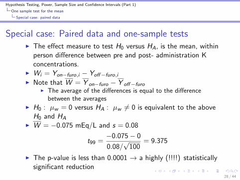
Special case: Paired data and one-sample testsI The effect measure to test H0 versus HA, is the mean, within
person difference between pre and post- administration Kconcentrations.
I Wi = Yon−furo,i − Yoff−furo,i
I Note that W = Y on−furo − Y off−furoI The average of the differences is equal to the difference
between the averagesI H0 : µw = 0 versus HA : µw 6= 0 is equivalent to the above
H0 and HA
I W = −0.075 mEq/L and s = 0.08
t99 =−0.075− 0
0.08/√
100= 9.375
I The p-value is less than 0.0001 → a highly (!!!!) statisticallysignificant reduction
28 / 44
Hypothesis Testing, Power, Sample Size and Confidence Intervals (Part 1)
One sample methods for a probability
Hypothesis testing
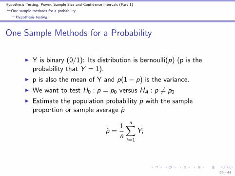
One Sample Methods for a Probability
I Y is binary (0/1): Its distribution is bernoulli(p) (p is theprobability that Y = 1).
I p is also the mean of Y and p(1− p) is the variance.
I We want to test H0 : p = p0 versus HA : p 6= p0
I Estimate the population probability p with the sampleproportion or sample average p̂
p̂ =1
n
n∑i=1
Yi
29 / 44
Hypothesis Testing, Power, Sample Size and Confidence Intervals (Part 1)
One sample methods for a probability
Hypothesis testing
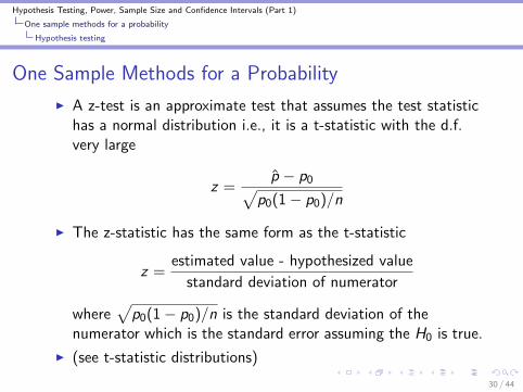
One Sample Methods for a Probability
I A z-test is an approximate test that assumes the test statistichas a normal distribution i.e., it is a t-statistic with the d.f.very large
z =p̂ − p0√
p0(1− p0)/n
I The z-statistic has the same form as the t-statistic
z =estimated value - hypothesized value
standard deviation of numerator
where√
p0(1− p0)/n is the standard deviation of thenumerator which is the standard error assuming the H0 is true.
I (see t-statistic distributions)
30 / 44
Hypothesis Testing, Power, Sample Size and Confidence Intervals (Part 1)
One sample methods for a probability
Hypothesis testing
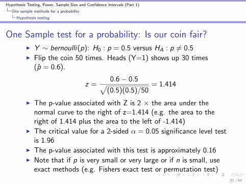
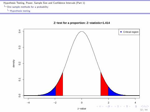
One Sample test for a probability: Is our coin fair?I Y ∼ bernoulli(p): H0 : p = 0.5 versus HA : p 6= 0.5I Flip the coin 50 times. Heads (Y=1) shows up 30 times
(p̂ = 0.6).
z =0.6− 0.5√
(0.5)(0.5)/50= 1.414
I The p-value associated with Z is 2 × the area under thenormal curve to the right of z=1.414 (e.g. the area to theright of 1.414 plus the area to the left of -1.414)
I The critical value for a 2-sided α = 0.05 significance level testis 1.96
I The p-value associated with this test is approximately 0.16I Note that if p is very small or very large or if n is small, use
exact methods (e.g. Fishers exact test or permutation test)
31 / 44
Hypothesis Testing, Power, Sample Size and Confidence Intervals (Part 1)
One sample methods for a probability
Hypothesis testing
−4 −2 0 2 4
0.0
0.1
0.2
0.3
0.4
Z−test for a proportion: Z−statistic=1.414
z−value
dens
ity
Critical region
32 / 44
Hypothesis Testing, Power, Sample Size and Confidence Intervals (Part 1)
One sample methods for a probability
Power, confidence intervals, and sample size
Power and confidence intervalsI Power increases when
I n increasesI p departs from p0
I p0 departs from 0.5
z =p̂ − p0√
p0(1− p0)/n
I Confidence intervalI 95%CI: (p̂ − 1.96 ·
√p̂(1− p̂/n, p̂ − 1.96 ·
√p̂(1− p̂/n)
I For the coin flipping example: p̂ = 0.6 and the 95% CI isgiven by
0.6± 1.96 ·√
0.6× 0.4/50 = (0.464, 0.736)
which is consistent with the 0.16 p-value that we hadobserved for H0 : p = 0.5.
33 / 44
Hypothesis Testing, Power, Sample Size and Confidence Intervals (Part 1)
Two sample tests for means
Hypothesis tests
Two sample test for means
I Two groups of patients (not paired)
I These are much more common than 1 sample tests
I We assume data come from a normal distribution (althoughthis is not completely necessary)
I For now, assume the two groups have equal variability inresponse distribution
I Test whether population means are equal
I Example: All patient in population 1 are treated withclonidine after limb amputation and all patients in population2 are treated with standard therapy.
I Scientific question:I What is the difference in the mean pain scale scores at 6
months following the amputation?
34 / 44
Hypothesis Testing, Power, Sample Size and Confidence Intervals (Part 1)
Two sample tests for means
Hypothesis tests
Two sample test for means
I H0 : µ1 = µ2 which can be generalized to H0 : µ1 − µ2 = 0or H0 : µ1 − µ2 = δ
I The quantity of interest (QOI) is µ1 − µ2
I If we want to test H0 : µ1 − µ2 = 0 and if we assume the twopopulations have equal variances, then the t- statistic is givenby:
t =point estimate of the QOI− 0
standard error of the numerator
I The estimate of the QOI: x1 − x2
35 / 44
Hypothesis Testing, Power, Sample Size and Confidence Intervals (Part 1)
Two sample tests for means
Hypothesis tests
Two sample test for means
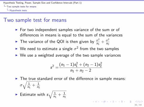
I For two independent samples variance of the sum or ofdifferences in means is equal to the sum of the variances
I The variance of the QOI is then given by σ2
n1+ σ2
n2
I We need to estimate a single σ2 from the two samples
I We use a weighted average of the two sample variances
s2 =(n1 − 1)s2
1 + (n2 − 1)s22
n1 + n2 − 2
I The true standard error of the difference in sample means:
σ√
1n1
+ 1n2
I Estimate with s√
1n1
+ 1n2
36 / 44
Hypothesis Testing, Power, Sample Size and Confidence Intervals (Part 1)
Two sample tests for means
Hypothesis tests
Two sample test for means
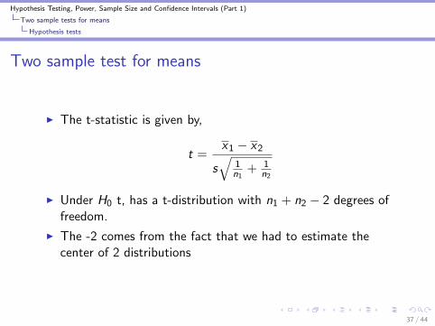
I The t-statistic is given by,
t =x1 − x2
s√
1n1
+ 1n2
I Under H0 t, has a t-distribution with n1 + n2 − 2 degrees offreedom.
I The -2 comes from the fact that we had to estimate thecenter of 2 distributions
37 / 44
Hypothesis Testing, Power, Sample Size and Confidence Intervals (Part 1)
Two sample tests for means
Hypothesis tests
Example: two sample test for means
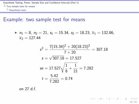
I n1 = 8, n2 = 21, s1 = 15.34, s2 = 18.23, x1 = 132.86,x2 = 127.44
s2 =7(15.34)2 + 20(18.23)2
7 + 20= 307.18
s =√
307.18 = 17.527
se = 17.527
√1
8+
1
21= 7.282
t =5.42
7.282= 0.74
on 27 d.f.
38 / 44
Hypothesis Testing, Power, Sample Size and Confidence Intervals (Part 1)
Two sample tests for means
Hypothesis tests
Example: two sample test for means
I The two-sided p-value is 0.466I You many verify with the surfstat.org t-distribution calculator
I The chance of getting a difference in means as large or largerthan 5.42 if the two populations have the same mean in 0.466.
I No evidence to suggest that the population means aredifferent.
39 / 44
Hypothesis Testing, Power, Sample Size and Confidence Intervals (Part 1)
Two sample tests for means
Power, confidence intervals, and sample size
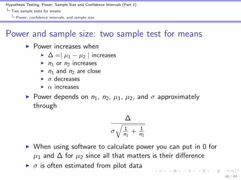
Power and sample size: two sample test for meansI Power increases when
I ∆ =| µ1 − µ2 | increasesI n1 or n2 increasesI n1 and n2 are closeI σ decreasesI α increases
I Power depends on n1, n2, µ1, µ2, and σ approximatelythrough
∆
σ√
1n1
+ 1n2
I When using software to calculate power you can put in 0 forµ1 and ∆ for µ2 since all that matters is their difference
I σ is often estimated from pilot data
40 / 44
Hypothesis Testing, Power, Sample Size and Confidence Intervals (Part 1)
Two sample tests for means
Power, confidence intervals, and sample size
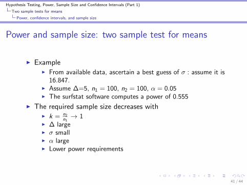
Power and sample size: two sample test for means
I ExampleI From available data, ascertain a best guess of σ : assume it is
16.847.I Assume ∆=5, n1 = 100, n2 = 100, α = 0.05I The surfstat software computes a power of 0.555
I The required sample size decreases withI k = n2
n1→ 1
I ∆ largeI σ smallI α largeI Lower power requirements
41 / 44
Hypothesis Testing, Power, Sample Size and Confidence Intervals (Part 1)
Two sample tests for means
Power, confidence intervals, and sample size
Power and sample size: two sample test for means
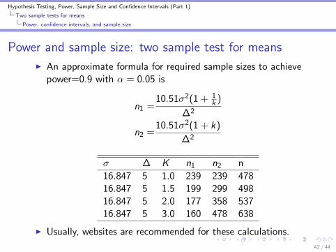
I An approximate formula for required sample sizes to achievepower=0.9 with α = 0.05 is
n1 =10.51σ2(1 + 1
k )
∆2
n2 =10.51σ2(1 + k)
∆2
σ ∆ K n1 n2 n
16.847 5 1.0 239 239 47816.847 5 1.5 199 299 49816.847 5 2.0 177 358 53716.847 5 3.0 160 478 638
I Usually, websites are recommended for these calculations.
42 / 44
Hypothesis Testing, Power, Sample Size and Confidence Intervals (Part 1)
Two sample tests for means
Power, confidence intervals, and sample size
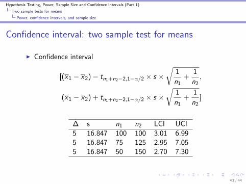
Confidence interval: two sample test for means
I Confidence interval
[(x1 − x2)− tn1+n2−2,1−α/2 × s ×√
1
n1+
1
n2,
(x1 − x2) + tn1+n2−2,1−α/2 × s ×√
1
n1+
1
n2]
∆ s n1 n2 LCI UCI
5 16.847 100 100 3.01 6.995 16.847 75 125 2.95 7.055 16.847 50 150 2.70 7.30
43 / 44
Hypothesis Testing, Power, Sample Size and Confidence Intervals (Part 1)
Two sample tests for means
Power, confidence intervals, and sample size
Summary
I Hypothesis testing, power, sample size, and confidenceintervals
I One sample test for the meanI One sample test for a probabilityI Two sample test for the mean
44 / 44
Recommended