*Corresponding Author’s Email: [email protected]
http://orcid.org/0000-0002-0782-0445
Landslide susceptibility assessment using statistical models: A case study in
Badulla district, Sri Lanka
G.J.M.S.R. Jayasinghe1*
, P. Wijekoon1 and J. Gunatilake
2
1Department of Statistics & Computer Science, Faculty of Science, University of Peradeniya, Sri Lanka
2Department of Geology, Faculty of Science, University of Peradeniya, Sri Lanka
Received:19/07/2017; Accepted:18/09/2017
Abstract:. Landslides are the most recurrent and
prominent natural hazard in many areas of the world
which cause significant loss of life and damage to
properties. By generating landslide susceptibility
maps, the hazard zones can be identified in order to
produce an early warning system to reduce the
damage. In this study, the predictive abilities of two
statistical models, Logistic regression (LR) model and
Geographically Weighted logistic regression (GWLR)
model, were compared. As a case study, a data set
collected for nine relevant causative factors over the
period from 1986 to 2014 was taken from Badulla
district, Sri Lanka, which is highly affected by
landslides. The performance of each model was tested
by using the Area under the curve (AUC) value of
Receiver operating characteristic curve (ROC), and
the GWLR model was selected as the best fitted
model. The probabilities obtained for each pixel in the
study area using the selected model were classified
into three classes (Low, Medium and High) based on
standard deviation method in GIS software. Finally, a
landslide susceptibility map was generated related to
the above three classes, from which high risk areas
can be identified to take necessary actions.
Keywords: Landslide, Susceptibility, Geographic
Information Systems (GIS), Geographically
Weighted logistic regression, Receiver operating
characteristic curve
INTRODUCTION
Landslide is defined as a “movement of mass of
soil or rock down a slope” (Courture, 2011), and
it is a common natural hazard in many areas of
the world. Annually landslides cause many
fatalities and property losses each year. In
addition, the damages can also caused on the
environment due to loss of wildlife and forest
cover. However, the damages to ecosystems due
to landslides cannot be easily estimated.
Therefore, landslide susceptibility analysis and
mapping are important to identify the landslide
hazard zones, and risk management can be
practiced to reduce the destruction to some
extent.
When identifying the factors which are
responsible for landslides, slope aspect, slope
angle and elevation of a location can be
considered as some key natural factors. Slope
aspect is the direction of a slope which identifies
the steepest downslope direction at a location.
Several researchers have shown the relationship
between aspect and landslide occurrence
(DeGraff and Romesburg, 1980, Marston et al.,
1998). Also, according to the knowledge of
experts, the probability of occurrence of
landslides is high when the slope angle is in
between 15 and 45 and it is relatively low
when it is more than 45 . Moreover, landslides
may occur in flat areas as well due to excessive
pressure placed on the respective area. The
elevation also affects the landslide occurrences,
since it determines the severity of climate
condition in mountain regions.
Slope curvature is another triggering
factor, which measures the rate of change of
slope. Using profile and plan curvature, the slope
curvature can be identified. The profile curvature
is the rate of change of slope parallel to slope
gradient. A negative value of profile curvature
implies that the surface is upwardly convex, a
positive profile conveys that the surface is
upwardly concave, and a value of zero indicates
that the surface is flat. Plan curvature is the rate
of change of slope perpendicular to slope
gradient which influences convergence and
divergence of flow. In this case, a positive value
implies that the surface is upwardly convex
whereas a negative value indicates the surface is
upwardly concave. Both profile and plan
curvature are two key factors responsible for
landslides since these factors affect the
Ceylon Journal of Science 46(4) 2017: 27-41
DOI: http://doi.org/10.4038/cjs.v46i4.7466
RESEARCH ARTICLE
28
Ceylon Journal of Science 46(4) 2017: 27-41
acceleration and deceleration of flow which
influences erosion.
Another key factor of landslide occurrence
is the landuse type due to human activity. The
data related to landuse can be extracted from
satellite images, and interpreted visually,
supported by supervised classification.
Theoretically, barren land and cultivations are
more prone to landslides. Further, the forest
areas tend to decrease landslide occurrences due
to the natural protection provided by the thick
vegetation cover.
Landslides may also occur on the slopes
intersected by roads. The cutting toe of the steep
slope, filling along the road and frequent
vibrations caused by vehicles are some human
activities in mountain areas that raise the
landslide susceptibility. According to Lee et al.
(2005), the potential of landslides also increases
with a decrease in distance to rivers. Therefore,
the distance to streams is another factor to be
considered in the susceptible landslide analyses.
Many qualitative and quantitative methods
are available to analyze data related to landslides.
The different approaches considered in the
literature can be identified as a heuristic,
physically-based modeling, probabilistic and
statistical. The heuristic approach is based on the
opinion of geomorphologic experts. Experts
define the weighting value for each causal factor
in this method. Determining exact weighting
values may cause incorrectness of results since
the method involves subject-oriented process. In
physically based modeling approach, slope
stability model is obtained by calculating safety
factor, and it is used to determine the landslide
hazard assessment. The probabilistic approach is
conducted by considering remote sensing data,
field observations, data collected from an
interview, and results based on historical
analysis. An obstacle to this method is that the
results do not present estimation of temporal
changes in landslide distribution. In the statistical
approach, the combinations of causal factors are
statistically determined and then forecasts future
landslide areas based on past landslides. Weights
of evidence method, Information value method,
Frequency ratio method, Logistic regression
analysis and discriminant analysis are some of
the methods that have been used under this
approach.
In recent years, there have been many
studies of landslide hazard mapping using
Geographic Information System (GIS), and most
of these studies have applied probabilistic
methods. Lee et al. (2005) have carried out
research on landslide susceptibility mapping in
Baguio City, Philippines using the frequency
ratio method, logistic regression and GIS. The
study was aimed to determine a relationship
between landslide occurrences and conditioning
factors, rating the predictors, and then to generate
the landslide susceptibility map using the
selected model and GIS.They identified landslide
locations using aerial photographs and field
surveys. The factors that they have considered
were the slope, aspect, curvature, the distance
from drainage, lithology, the distance from fault
and land cover. The results were finally validated
using known landslide locations, and it was
found that the logistic regression model had
higher predictive value (80 %) than that of the
frequency ratio method (78.4%).
Modeling of road related and non-road
related landslide hazard for a large geographical
area was carried out by Gorsevski et al. (2006)
by using logistic regression and receiver
operating characteristic (ROC) analysis. The
variables selected for this study were elevation,
slope, aspect, profile curvature, plan curvature,
tangent curve, flow path length, and upslope
area. The landslide data set was subdivided to
road related, and non-road related landslides and
two separate logistic regression models were
obtained and compared. It was noted that spatial
prediction and predictor variables for those
models were different. Using ROC method, the
performance of the predictive rule of two models
was measured.
Dieu et al. (2012) have conducted research
on landslide susceptibility assessment in
Vietnam by using three methods; data mining
approaches, the support vector machines (SVM),
and Decision Tree (DT) and Naïve Bayes (NB)
models. They have used a landslide inventory
having 118 landslides records, and then
partitioned it randomly into 70% as training
dataset and remaining data to validate results.
Landslide susceptibility index was calculated by
considering slope angle, slope aspect, relief
amplitude, lithology, soil type, land use, distance
to roads, distance to rivers, distance to faults and
rainfall as landslide causal factors. Finally,
based on validation results and landslide
29
Jayasinghe et al.
susceptibility maps, it was shown that SVM is a
powerful tool for landslide susceptibility
assessment with high accuracy with compared to
other two methods.
The main objective of this study is to
assess and evaluate the landslide susceptibility
using two types of statistical models; logistic
regression (LR) model, which is mostly used in
literature, and Geographical Weighted logistic
regression (GWLR) model to address the spatial
variability, respectively. These two methods
were applied to a dataset gathered from Badulla
district, Sri Lanka.
MATERIALS AND METHODS
Study Area
Sri Lanka is situated in Asia-Pacific region, and
is located at the northern latitude of 50 55‟ and 9
0
51‟ and eastern longitude of 790 41‟ and 81
0 53‟,
having an area of 65,610 km2. There are 25
districts organized into 9 provinces in the
country. According to the statistics, Asia-Pacific
region is considered as one of the most disaster-
prone regions in the world (Report on disaster
mitigation in Asia and the Pacific, 1991), since
landslides in Sri Lanka spread over about 30% of
land area and into several districts namely
Badulla, Nuwareliya, Matara, and Kandy etc.
In 1986, 51 lives were lost and
approximately 10,000 families were displaced in
Sri Lanka as a result of landslides. In a most
recent incident occurred in 2014, 13 died, and
1,875 were affected in Meeriyabedda in Badulla
district. These natural disasters cause major
threats to the country‟s economy through
significant losses of life, infrastructure and crops,
etc. in every year. The National Building
Research Organization (NBRO) in Sri Lanka is
currently preparing maps which illustrate the
distribution of landslides prone districts via
Geographic Information System (GIS). To draw
these maps they use qualitative methods which
assign weights for causative factors on expert‟s
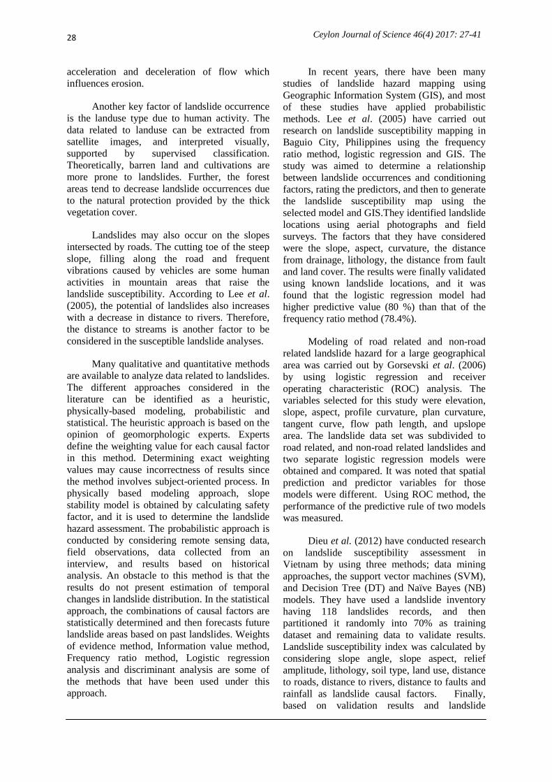
knowledge. Figure 1 shows the spatial
distribution of landslides in Sri Lanka from 1974
to 2008. According to this figure, it is clear that
Badulla district is more prone for landslides
compared to other districts in Sri Lanka.
Therefore, Badulla District was selected as the
study area which is situated in 6°59‟05”N and
81°03‟23”E, and encompasses approximately
about 2861km2
area. Fifteen district secretariat
(DS) divisions (Bandarawela, Uvaparanagama,
Ella, Welimada, Hali-Ela, Passara, Haldummulla,
Lunugala, Kandaketiya, Haputhale, Soranathota,
Badulla, Meegahakivula, Ridimaliyadda,
Mahiyangana) are in this district, and cultivation
is the predominant occupation of the people in
the area.
Figure 1: Spatial distribution of landslides in Sri Lanka from 1974 to 2008, Source: Sri Lanka National Report on Disaster
Risk, Poverty and Human Relationships.
30
Ceylon Journal of Science 46(4) 2017: 27-41
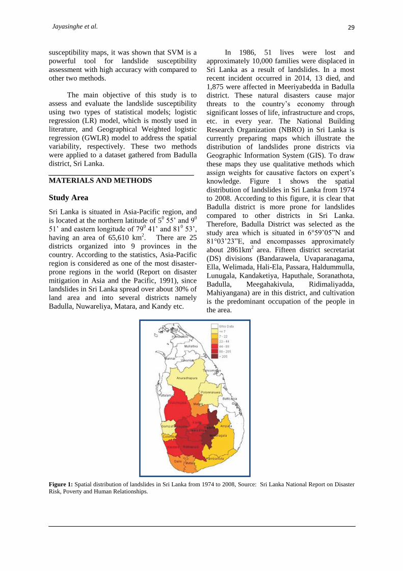
Data Collection
The landslide location map [Figure 2 (a)], the
soil map, contour map, landuse map, stream map
and road network map [Figure 2 (b)] were
collected form the NBRO, Survey Department
and Natural Resource Management Centre
(NRMC). The starting points of landslides based
on the sample location map in the study area
from 1986 to 2014 were used for the analysis.
The maps including soil, contour, landuse,
stream and road network maps were as of 2014.
By following Dieu et al. (2012), the values
for the predictor variables for each of the
landslide starting points have been obtained
based on the current environment.
Based on the classification of NRMC, five
types of landuse, namely cultivated areas, built-
up areas, bare areas, rock lands and other types,
and 11 soil types were identified in the study
area (Table 1).
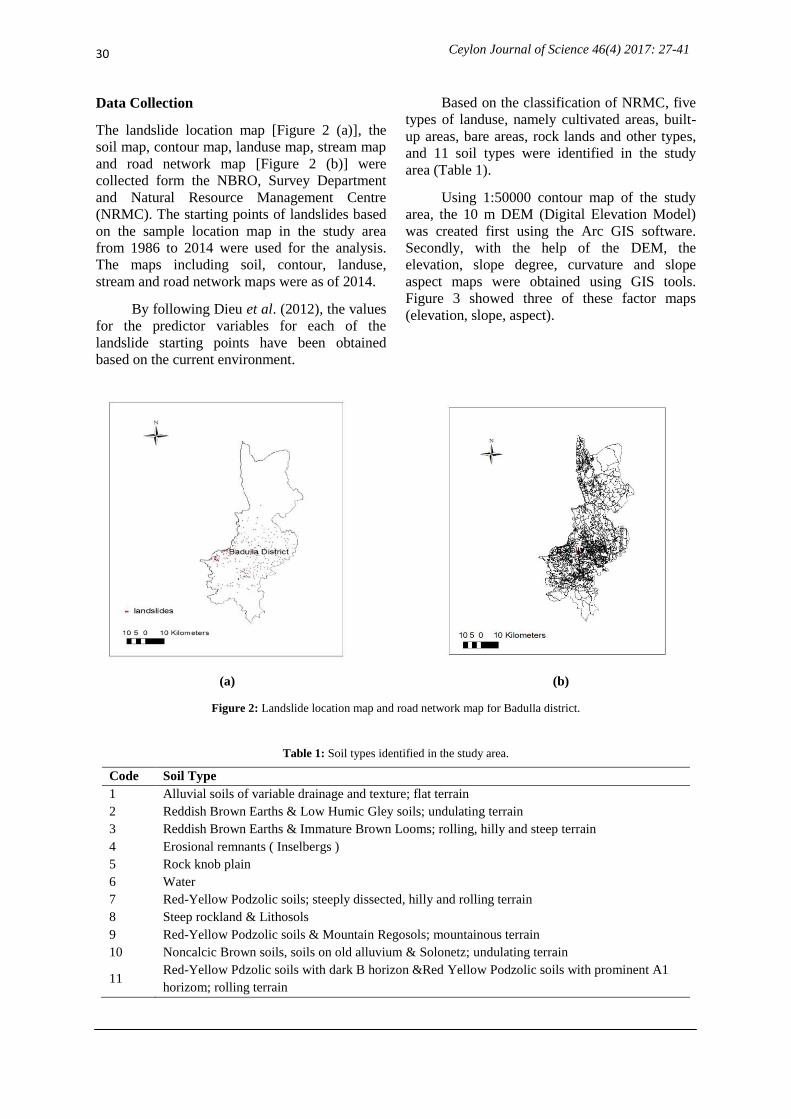
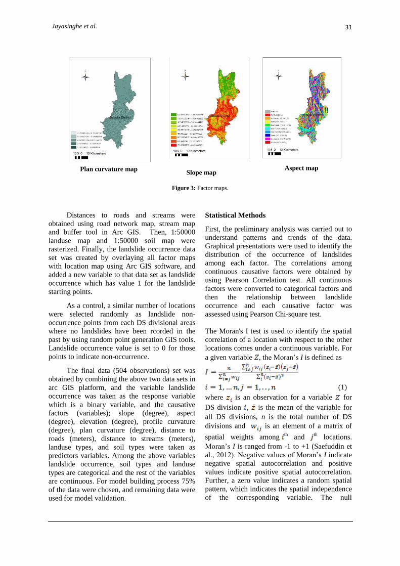
Using 1:50000 contour map of the study
area, the 10 m DEM (Digital Elevation Model)
was created first using the Arc GIS software.
Secondly, with the help of the DEM, the
elevation, slope degree, curvature and slope
aspect maps were obtained using GIS tools.
Figure 3 showed three of these factor maps
(elevation, slope, aspect).
Figure 2: Landslide location map and road network map for Badulla district.
Table 1: Soil types identified in the study area.
Code Soil Type
1 Alluvial soils of variable drainage and texture; flat terrain
2 Reddish Brown Earths & Low Humic Gley soils; undulating terrain
3 Reddish Brown Earths & Immature Brown Looms; rolling, hilly and steep terrain
4 Erosional remnants ( Inselbergs )
5 Rock knob plain
6 Water
7 Red-Yellow Podzolic soils; steeply dissected, hilly and rolling terrain
8 Steep rockland & Lithosols
9 Red-Yellow Podzolic soils & Mountain Regosols; mountainous terrain
10 Noncalcic Brown soils, soils on old alluvium & Solonetz; undulating terrain
11 Red-Yellow Pdzolic soils with dark B horizon &Red Yellow Podzolic soils with prominent A1
horizom; rolling terrain
(b) (a)
31
Jayasinghe et al.
Figure 3: Factor maps.
Distances to roads and streams were
obtained using road network map, stream map
and buffer tool in Arc GIS. Then, 1:50000
landuse map and 1:50000 soil map were
rasterized. Finally, the landslide occurrence data
set was created by overlaying all factor maps
with location map using Arc GIS software, and
added a new variable to that data set as landslide
occurrence which has value 1 for the landslide
starting points.
As a control, a similar number of locations
were selected randomly as landslide non-
occurrence points from each DS divisional areas
where no landslides have been rcorded in the
past by using random point generation GIS tools.
Landslide occurrence value is set to 0 for those
points to indicate non-occurrence.
The final data (504 observations) set was
obtained by combining the above two data sets in
arc GIS platform, and the variable landslide
occurrence was taken as the response variable
which is a binary variable, and the causative
factors (variables); slope (degree), aspect
(degree), elevation (degree), profile curvature
(degree), plan curvature (degree), distance to
roads (meters), distance to streams (meters),
landuse types, and soil types were taken as
predictors variables. Among the above variables
landslide occurrence, soil types and landuse
types are categorical and the rest of the variables
are continuous. For model building process 75%
of the data were chosen, and remaining data were
used for model validation.
Statistical Methods
First, the preliminary analysis was carried out to
understand patterns and trends of the data.
Graphical presentations were used to identify the
distribution of the occurrence of landslides
among each factor. The correlations among
continuous causative factors were obtained by
using Pearson Correlation test. All continuous
factors were converted to categorical factors and
then the relationship between landslide
occurrence and each causative factor was
assessed using Pearson Chi-square test.
The Moran's I test is used to identify the spatial
correlation of a location with respect to the other
locations comes under a continuous variable. For
a given variable , the Moran‟s I is defined as
(1)
where is an observation for a variable for
DS division , is the mean of the variable for
all DS divisions, n is the total number of DS
divisions and is an element of a matrix of
spatial weights amongth and
th locations.
Moran‟s I is ranged from -1 to +1 (Saefuddin et
al., 2012). Negative values of Moran‟s I indicate
negative spatial autocorrelation and positive
values indicate positive spatial autocorrelation.
Further, a zero value indicates a random spatial
pattern, which indicates the spatial independence
of the corresponding variable. The null
Aspect map Plan curvature map Slope map
32
Ceylon Journal of Science 46(4) 2017: 27-41
hypothesis of this Moran‟s I test is that there is
no spatial correlation.
In this study, two types of statistical
models were fitted and their performances were
compared. The first model is the Logistic
Regression (LR) model for which the predictor
variables are assumed to be uncorrelated. R
software was used for this analysis. If a spatial
correlation exists among predictor variables the
second model, the Geographical Weighted
logistic regression (GWLR) (Brunsdon et al.,
1996) can be used. In both models the response
variable is a binary variable which represents the
occurrence or non-occurrence of landslides.
The LR model is given by
(2)
where is the probability of occurrence of
landslides, is the th predictor variable, is
the intercept, and is the coefficient of the th
predictor variable. The maximum likelihood
(ML) method was used to estimate unknown coefficients. The ML estimator for coefficients
can be obtained by maximizing the likelihood
function. The significance of each estimated
coefficient was assessed using Wald test at a
given significance level. To select the best fitted
model the backward elimination method was
applied by following Gorsevski et al. (2006).
The Geographical Weighted logistic regression
(GWLR) model given below is used to
incorporate the spatial correlation.
(3)
where and are local model parameters
specific to a location at ( ) coordinate.
According to this method, separate models are
fitted for each selected location, and model
parameters are defined as specific to the location.
When estimating parameters at a particular
location, a weight is given to each data point in
the sample such that the observations near to that
location are given greater weight than
observations further away.
Several methods are available to determine
weighting function of GWLR for estimating
parameters (Saefuddin et al., 2012). The
weighting function used in this study is called the
spatially adaptive weighting scheme
(Fotheringham et al., 2002), and it is defined as
follows:
(4)
where is the distance between locations and
, and is the bandwidth. To select the optimum
bandwidth, the Corrected Akaike Information
Criterion (AICc) is adapted.
According to Fotheringham et al. (2002), the
local t test shown below assesses the spatial
variability of the predictor variables. The test
statistics of the local t test is
(5)
where is the standard error of for the
jth
parameter estimates. According to this test the
local parameter estimates of GWLR model has a
significant spatial variation when > 2 and/or
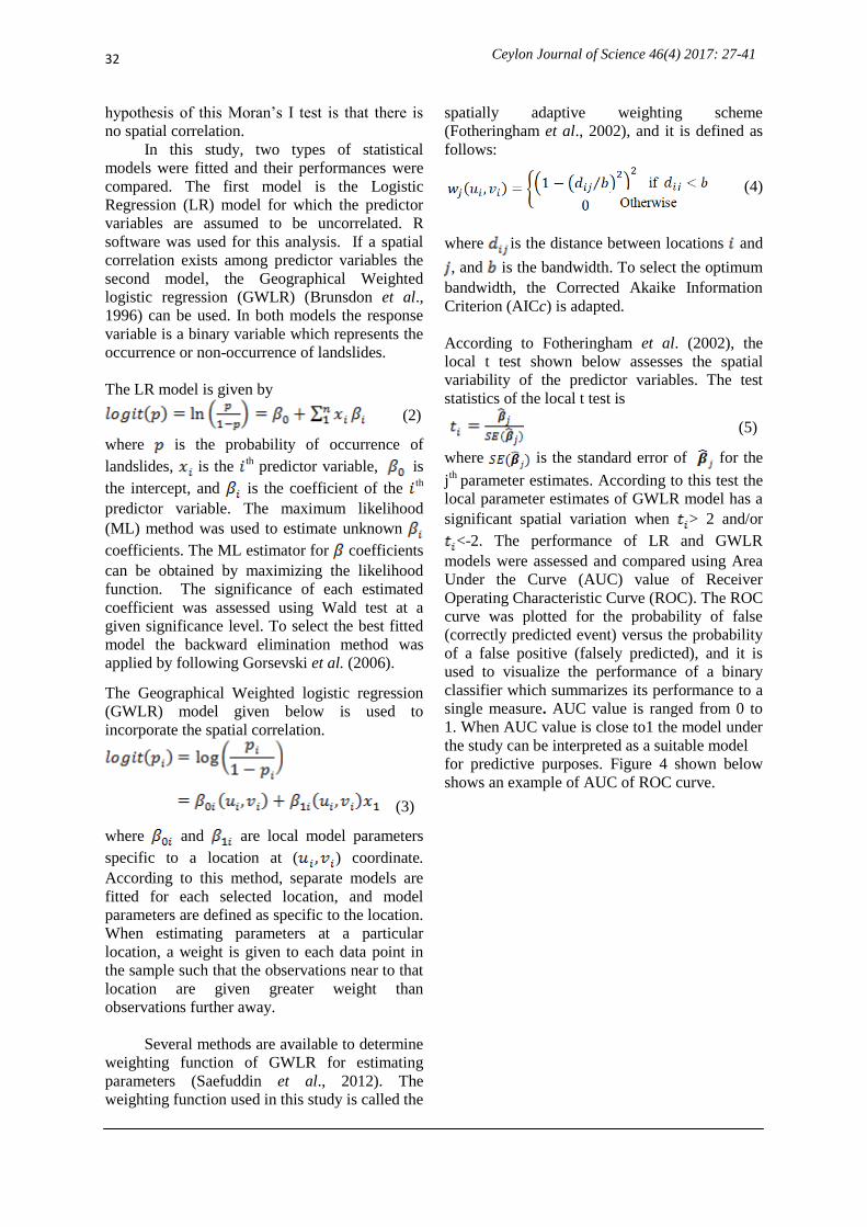
<-2. The performance of LR and GWLR
models were assessed and compared using Area
Under the Curve (AUC) value of Receiver
Operating Characteristic Curve (ROC). The ROC
curve was plotted for the probability of false
(correctly predicted event) versus the probability
of a false positive (falsely predicted), and it is
used to visualize the performance of a binary
classifier which summarizes its performance to a
single measure. AUC value is ranged from 0 to
1. When AUC value is close to1 the model under
the study can be interpreted as a suitable model
for predictive purposes. Figure 4 shown below
shows an example of AUC of ROC curve.
33
Jayasinghe et al.
Figure 4 : ROC curves.
Figure 4(a) depicts the ROC curve of an almost
perfect classifier where the performance curve
almost touches the „perfect performance‟ point in
the top left corner. The performance of model
related to Figure 4(b) is higher than that
represents in Figure 4(c).
Based on AUC of ROC curve the best
model was selected, and then using GIS, for each
pixel in the study area the probability of
landslide occurrence was calculated. The
Standard deviation classification method (Esri,
2015) in Arc GIS was used to obtain
susceptibility classes to draw maps. In this
method first the mean () and standard deviation
() of predicted probabilities, related to the
events of landslide occurrences, are taken to
obtain three susceptibility classes (low, medium,
high).Class breaks are created with equal ranges.
According Esri (2015), these ranges are usually
based on intervals of 1, ½, ⅓, or ¼ standard
deviations using mean values and the standard
deviations from the mean. Here it was considered
½ standard deviation. Finally, the landslide
susceptibility map was drawn for the study area
using these classified probabilities.
RESULTS AND DISCUSSION
Preliminary Analysis
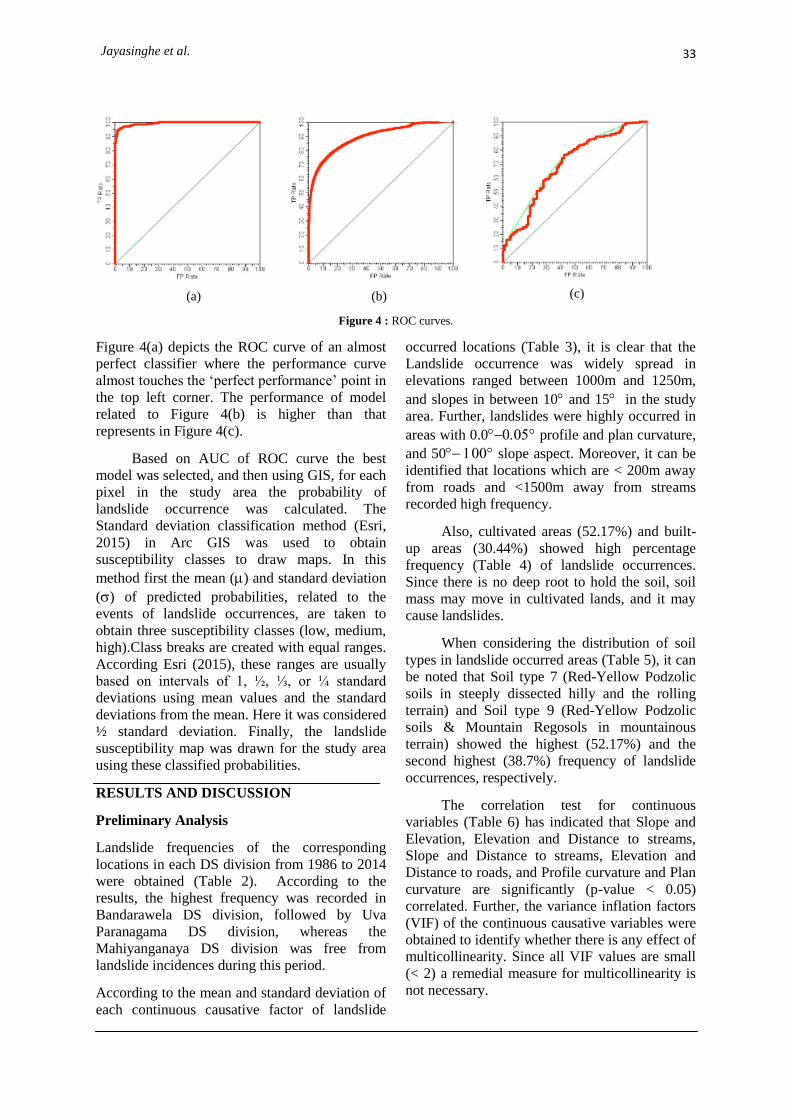
Landslide frequencies of the corresponding
locations in each DS division from 1986 to 2014
were obtained (Table 2). According to the
results, the highest frequency was recorded in
Bandarawela DS division, followed by Uva
Paranagama DS division, whereas the
Mahiyanganaya DS division was free from
landslide incidences during this period.
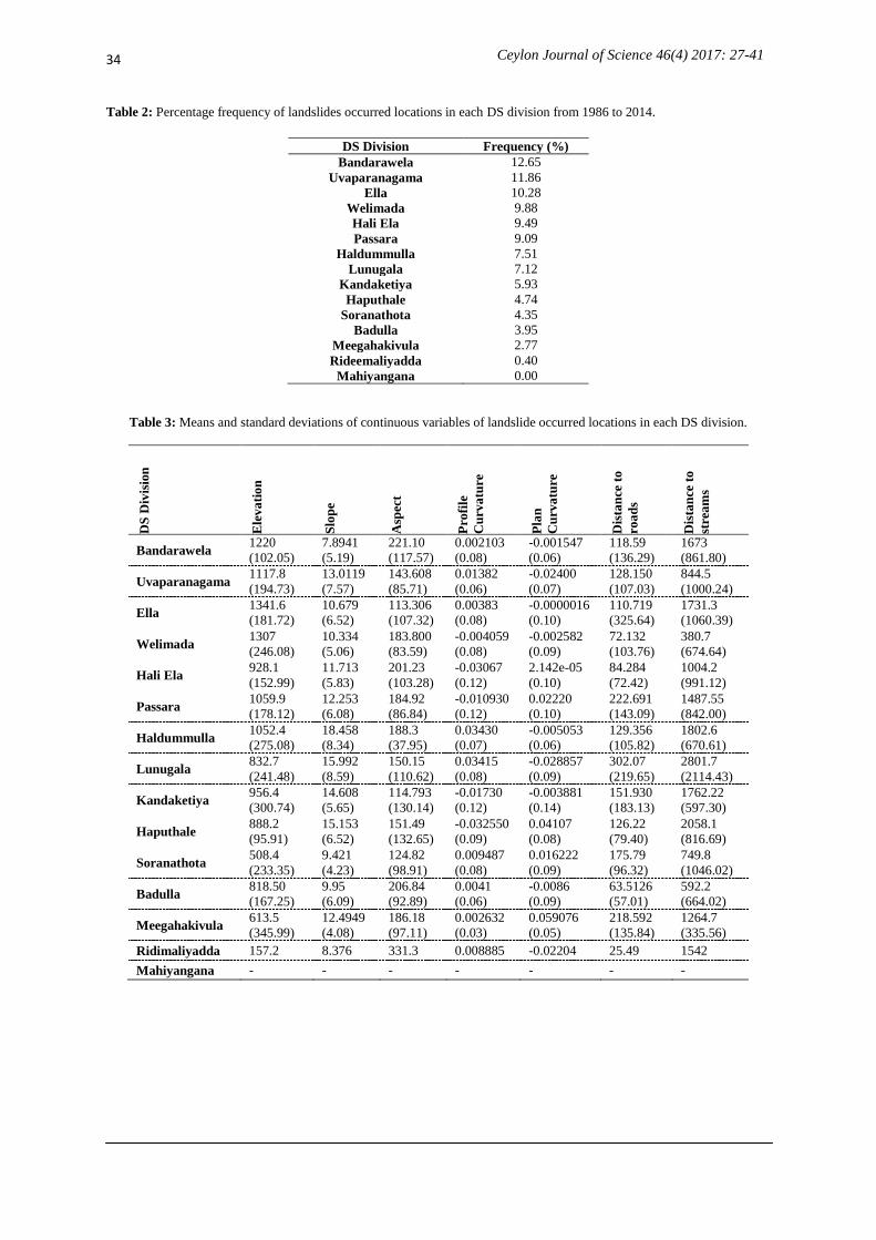
According to the mean and standard deviation of
each continuous causative factor of landslide
occurred locations (Table 3), it is clear that the
Landslide occurrence was widely spread in
elevations ranged between 1000m and 1250m,
and slopes in between 10 and 15 in the study
area. Further, landslides were highly occurred in
areas with 0.0 profile and plan curvature,
and 50 slope aspect. Moreover, it can be
identified that locations which are < 200m away
from roads and <1500m away from streams
recorded high frequency.
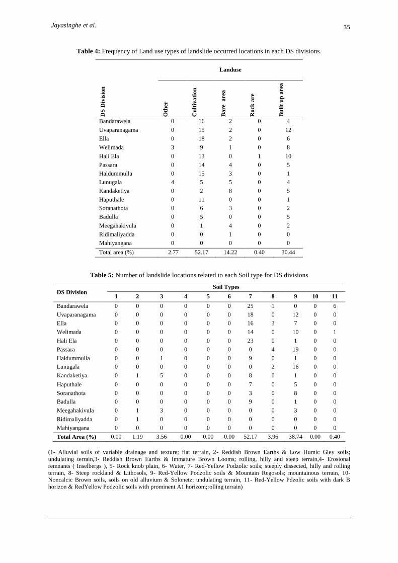
Also, cultivated areas (52.17%) and built-
up areas (30.44%) showed high percentage
frequency (Table 4) of landslide occurrences.
Since there is no deep root to hold the soil, soil
mass may move in cultivated lands, and it may
cause landslides.
When considering the distribution of soil
types in landslide occurred areas (Table 5), it can
be noted that Soil type 7 (Red-Yellow Podzolic
soils in steeply dissected hilly and the rolling
terrain) and Soil type 9 (Red-Yellow Podzolic
soils & Mountain Regosols in mountainous
terrain) showed the highest (52.17%) and the
second highest (38.7%) frequency of landslide
occurrences, respectively.
The correlation test for continuous
variables (Table 6) has indicated that Slope and
Elevation, Elevation and Distance to streams,
Slope and Distance to streams, Elevation and
Distance to roads, and Profile curvature and Plan
curvature are significantly (p-value < 0.05)
correlated. Further, the variance inflation factors
(VIF) of the continuous causative variables were
obtained to identify whether there is any effect of
multicollinearity. Since all VIF values are small
(< 2) a remedial measure for multicollinearity is
not necessary.
(a) (b) (c)
34
Ceylon Journal of Science 46(4) 2017: 27-41
Table 2: Percentage frequency of landslides occurred locations in each DS division from 1986 to 2014.
DS Division Frequency (%)
Bandarawela 12.65
Uvaparanagama 11.86
Ella 10.28
Welimada 9.88
Hali Ela 9.49
Passara 9.09
Haldummulla 7.51
Lunugala 7.12
Kandaketiya 5.93
Haputhale 4.74
Soranathota 4.35
Badulla 3.95
Meegahakivula 2.77
Rideemaliyadda 0.40
Mahiyangana 0.00
Table 3: Means and standard deviations of continuous variables of landslide occurred locations in each DS division.
DS
Div
isio
n
Ele
va
tio
n
Slo
pe
Asp
ect
Pro
file
Cu
rva
ture
Pla
n
Cu
rva
ture
Dis
tan
ce t
o
roa
ds
Dis
tan
ce t
o
stre
am
s
Bandarawela 1220
(102.05)
7.8941
(5.19)
221.10
(117.57)
0.002103
(0.08)
-0.001547
(0.06)
118.59
(136.29)
1673
(861.80)
Uvaparanagama 1117.8
(194.73)
13.0119
(7.57)
143.608
(85.71)
0.01382
(0.06)
-0.02400
(0.07)
128.150
(107.03)
844.5
(1000.24)
Ella 1341.6
(181.72)
10.679
(6.52)
113.306
(107.32)
0.00383
(0.08)
-0.0000016
(0.10)
110.719
(325.64)
1731.3
(1060.39)
Welimada 1307
(246.08)
10.334
(5.06)
183.800
(83.59)
-0.004059
(0.08)
-0.002582
(0.09)
72.132
(103.76)
380.7
(674.64)
Hali Ela 928.1
(152.99)
11.713
(5.83)
201.23
(103.28)
-0.03067
(0.12)
2.142e-05
(0.10)
84.284
(72.42)
1004.2
(991.12)
Passara 1059.9
(178.12)
12.253
(6.08)
184.92
(86.84)
-0.010930
(0.12)
0.02220
(0.10)
222.691
(143.09)
1487.55
(842.00)
Haldummulla 1052.4
(275.08)
18.458
(8.34)
188.3
(37.95)
0.03430
(0.07)
-0.005053
(0.06)
129.356
(105.82)
1802.6
(670.61)
Lunugala 832.7
(241.48)
15.992
(8.59)
150.15
(110.62)
0.03415
(0.08)
-0.028857
(0.09)
302.07
(219.65)
2801.7
(2114.43)
Kandaketiya 956.4
(300.74)
14.608
(5.65)
114.793
(130.14)
-0.01730
(0.12)
-0.003881
(0.14)
151.930
(183.13)
1762.22
(597.30)
Haputhale 888.2
(95.91)
15.153
(6.52)
151.49
(132.65)
-0.032550
(0.09)
0.04107
(0.08)
126.22
(79.40)
2058.1
(816.69)
Soranathota 508.4
(233.35)
9.421
(4.23)
124.82
(98.91)
0.009487
(0.08)
0.016222
(0.09)
175.79
(96.32)
749.8
(1046.02)
Badulla 818.50
(167.25)
9.95
(6.09)
206.84
(92.89)
0.0041
(0.06)
-0.0086
(0.09)
63.5126
(57.01)
592.2
(664.02)
Meegahakivula 613.5
(345.99)
12.4949
(4.08)
186.18
(97.11)
0.002632
(0.03)
0.059076
(0.05)
218.592
(135.84)
1264.7
(335.56)
Ridimaliyadda 157.2 8.376 331.3 0.008885 -0.02204 25.49 1542
Mahiyangana - - - - - - -
35
Jayasinghe et al.
Table 4: Frequency of Land use types of landslide occurred locations in each DS divisions.
DS
Div
isio
n
Landuse
Oth
er
Cu
ltiv
ati
on
Ba
re
are
a
Ro
ck a
re
Bu
ilt
up
are
a
Bandarawela 0 16 2 0 4
Uvaparanagama 0 15 2 0 12
Ella 0 18 2 0 6
Welimada 3 9 1 0 8
Hali Ela 0 13 0 1 10
Passara 0 14 4 0 5
Haldummulla 0 15 3 0 1
Lunugala 4 5 5 0 4
Kandaketiya 0 2 8 0 5
Haputhale 0 11 0 0 1
Soranathota 0 6 3 0 2
Badulla 0 5 0 0 5
Meegahakivula 0 1 4 0 2
Ridimaliyadda 0 0 1 0 0
Mahiyangana 0 0 0 0 0
Total area (%) 2.77 52.17 14.22 0.40 30.44
Table 5: Number of landslide locations related to each Soil type for DS divisions
DS Division Soil Types
1 2 3 4 5 6 7 8 9 10 11
Bandarawela 0 0 0 0 0 0 25 1 0 0 6
Uvaparanagama 0 0 0 0 0 0 18 0 12 0 0
Ella 0 0 0 0 0 0 16 3 7 0 0
Welimada 0 0 0 0 0 0 14 0 10 0 1
Hali Ela 0 0 0 0 0 0 23 0 1 0 0
Passara 0 0 0 0 0 0 0 4 19 0 0
Haldummulla 0 0 1 0 0 0 9 0 1 0 0
Lunugala 0 0 0 0 0 0 0 2 16 0 0
Kandaketiya 0 1 5 0 0 0 8 0 1 0 0
Haputhale 0 0 0 0 0 0 7 0 5 0 0
Soranathota 0 0 0 0 0 0 3 0 8 0 0
Badulla 0 0 0 0 0 0 9 0 1 0 0
Meegahakivula 0 1 3 0 0 0 0 0 3 0 0
Ridimaliyadda 0 1 0 0 0 0 0 0 0 0 0
Mahiyangana 0 0 0 0 0 0 0 0 0 0 0
Total Area (%) 0.00 1.19 3.56 0.00 0.00 0.00 52.17 3.96 38.74 0.00 0.40
(1- Alluvial soils of variable drainage and texture; flat terrain, 2- Reddish Brown Earths & Low Humic Gley soils;
undulating terrain,3- Reddish Brown Earths & Immature Brown Looms; rolling, hilly and steep terrain,4- Erosional
remnants ( Inselbergs ), 5- Rock knob plain, 6- Water, 7- Red-Yellow Podzolic soils; steeply dissected, hilly and rolling
terrain, 8- Steep rockland & Lithosols, 9- Red-Yellow Podzolic soils & Mountain Regosols; mountainous terrain, 10-
Noncalcic Brown soils, soils on old alluvium & Solonetz; undulating terrain, 11- Red-Yellow Pdzolic soils with dark B
horizon & RedYellow Podzolic soils with prominent A1 horizom;rolling terrain)
36
Ceylon Journal of Science 46(4) 2017: 27-41
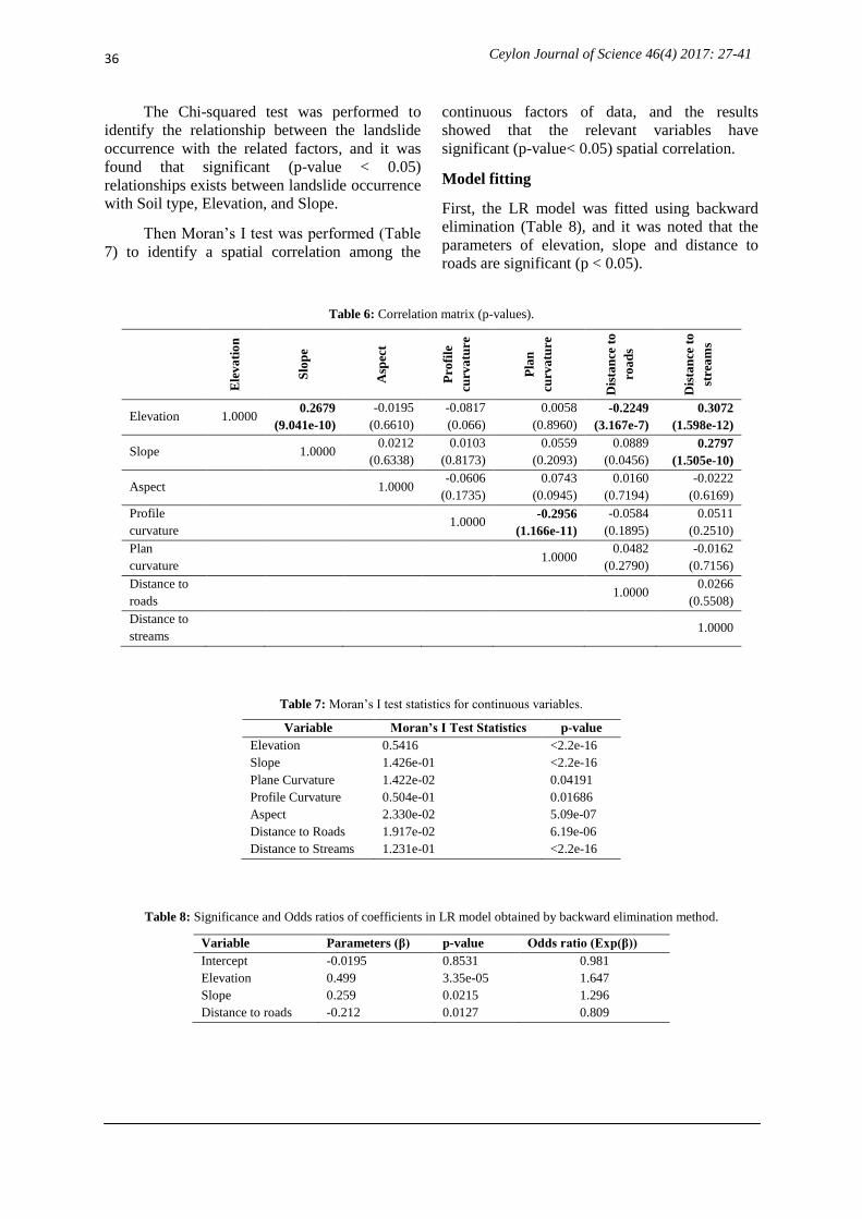
The Chi-squared test was performed to
identify the relationship between the landslide
occurrence with the related factors, and it was
found that significant (p-value < 0.05)
relationships exists between landslide occurrence
with Soil type, Elevation, and Slope.
Then Moran‟s I test was performed (Table
7) to identify a spatial correlation among the
continuous factors of data, and the results
showed that the relevant variables have
significant (p-value< 0.05) spatial correlation.
Model fitting
First, the LR model was fitted using backward
elimination (Table 8), and it was noted that the
parameters of elevation, slope and distance to
roads are significant (p < 0.05).
Table 6: Correlation matrix (p-values).
Ele
va
tio
n
Slo
pe
Asp
ect
Pro
file
curv
atu
re
Pla
n
curv
atu
re
Dis
tan
ce t
o
roa
ds
Dis
tan
ce t
o
stre
am
s
Elevation 1.0000 0.2679
(9.041e-10)
-0.0195
(0.6610)
-0.0817
(0.066)
0.0058
(0.8960)
-0.2249
(3.167e-7)
0.3072
(1.598e-12)
Slope 1.0000 0.0212
(0.6338)
0.0103
(0.8173)
0.0559
(0.2093)
0.0889
(0.0456)
0.2797
(1.505e-10)
Aspect 1.0000 -0.0606
(0.1735)
0.0743
(0.0945)
0.0160
(0.7194)
-0.0222
(0.6169)
Profile
curvature 1.0000
-0.2956
(1.166e-11)
-0.0584
(0.1895)
0.0511
(0.2510)
Plan
curvature 1.0000
0.0482
(0.2790)
-0.0162
(0.7156)
Distance to
roads 1.0000
0.0266
(0.5508)
Distance to
streams 1.0000
Table 7: Moran‟s I test statistics for continuous variables.
Variable Moran’s I Test Statistics p-value
Elevation 0.5416 <2.2e-16
Slope 1.426e-01 <2.2e-16
Plane Curvature 1.422e-02 0.04191
Profile Curvature 0.504e-01 0.01686
Aspect 2.330e-02 5.09e-07
Distance to Roads 1.917e-02 6.19e-06
Distance to Streams 1.231e-01 <2.2e-16
Table 8: Significance and Odds ratios of coefficients in LR model obtained by backward elimination method.
Variable Parameters (β) p-value Odds ratio (Exp(β))
Intercept -0.0195 0.8531 0.981
Elevation 0.499 3.35e-05 1.647
Slope 0.259 0.0215 1.296
Distance to roads -0.212 0.0127 0.809
37
Jayasinghe et al.
The fitted model with estimated parameters is given below.
(6)
where is a binary variable such that for
non-occurrence of landslides and for
occurrence of landslides. Note that when
elevation and slope increase, the probability of
landslide occurrence also increases since
elevation and slope are positively related to the
response variable . According to the odds ratio,
it was noted that when one unit of the elevation
increases, odds of a landslide occurrence
increases by 64.7%. Moreover, it can be
identified that odds of landslide occurrence
increases by 29.6% when one unit of the slope
increases. Further, it was shown that the variable
distance to roads negatively affects, and as
increasing of one unit of the distance to roads,
odds of landslide occurrence decreases by
80.9%.
Since the causative factors have significant
(p-value < 0.05) spatial correlation according to
the Moran‟s I test, the GWLR model was fitted
to incorporate this spatial relationship by using
GWR4 software. Using this method a local
model for each location in the sample was fitted
by considering the neighbourhood area, and the
minimum AICc criterion was used to obtain the
optimal bandwidth size which is 102.0 m for the
selected model.
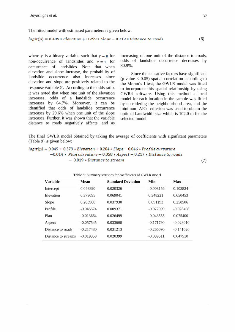
The final GWLR model obtained by taking the average of coefficients with significant parameters
(Table 9) is given below:
(7)
Table 9: Summary statistics for coefficients of GWLR model.
Variable Mean Standard Deviation Min Max
Intercept 0.048890 0.020326 -0.008156 0.103824
Elevation 0.379095 0.069041 0.348221 0.650453
Slope 0.203980 0.037930 0.091193 0.258506
Profile -0.045574 0.009371 -0.072999 -0.028498
Plan -0.013664 0.026499 -0.043555 0.075400
Aspect -0.057545 0.033600 -0.171790 -0.028010
Distance to roads -0.217480 0.031213 -0.266090 -0.141626
Distance to streams -0.019358 0.020399 -0.039511 0.047510
38
Ceylon Journal of Science 46(4) 2017: 27-41
In the above equation, elevation, slope and
distance to roads have higher coefficients with
compared to the other variables which indicate
that these three variables have high impact with
landslide occurrences. To assess whether the
spatial variation in the measured relationship is
substantial, the geographically variability t-test
(Table 10) was applied to each estimate of
parameters of the selected model.
Note that the values of the test statistics
from elevation up to Plan curvature are less than
-2 and from Profile curvature to Distance to
streams are greater than 2. This implies that there
exists a significant spatial variation in each
coefficient.
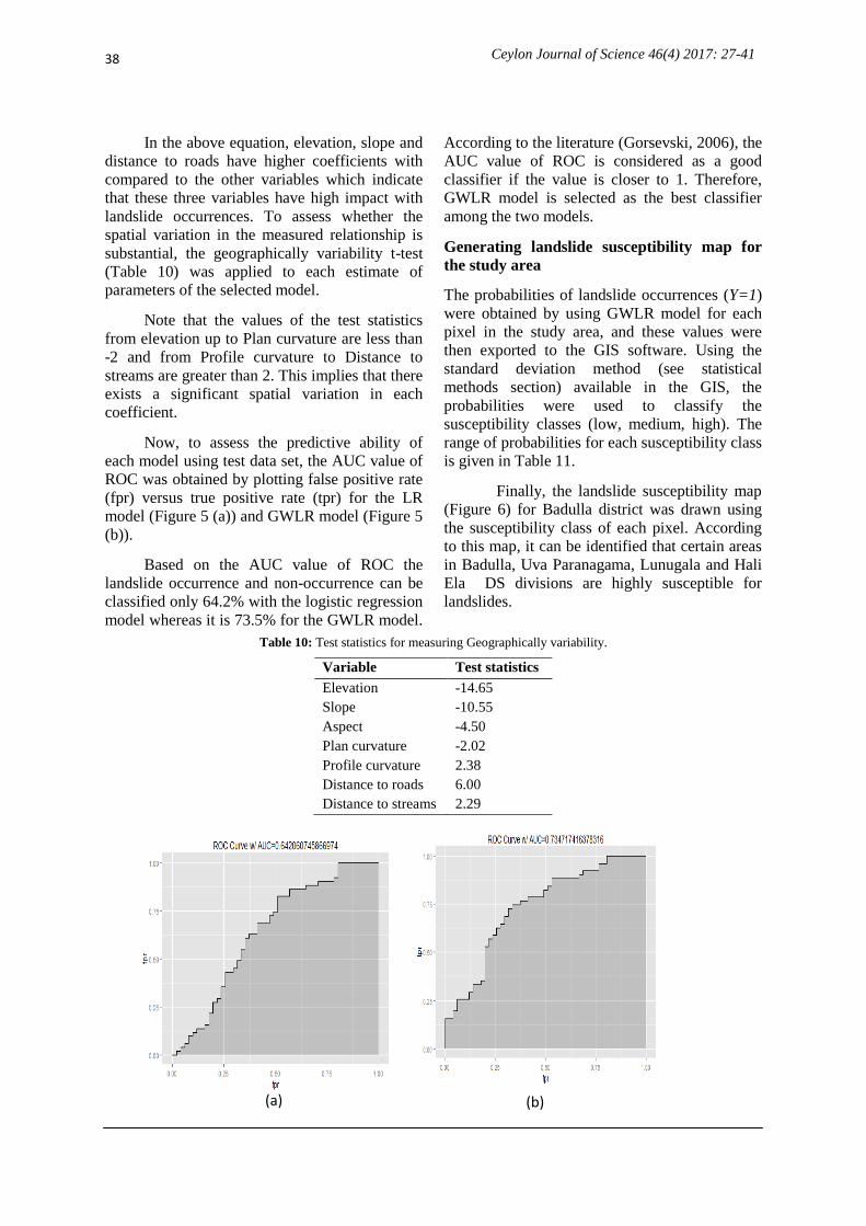
Now, to assess the predictive ability of
each model using test data set, the AUC value of
ROC was obtained by plotting false positive rate
(fpr) versus true positive rate (tpr) for the LR
model (Figure 5 (a)) and GWLR model (Figure 5
(b)).
Based on the AUC value of ROC the
landslide occurrence and non-occurrence can be
classified only 64.2% with the logistic regression
model whereas it is 73.5% for the GWLR model.
According to the literature (Gorsevski, 2006), the
AUC value of ROC is considered as a good
classifier if the value is closer to 1. Therefore,
GWLR model is selected as the best classifier
among the two models.
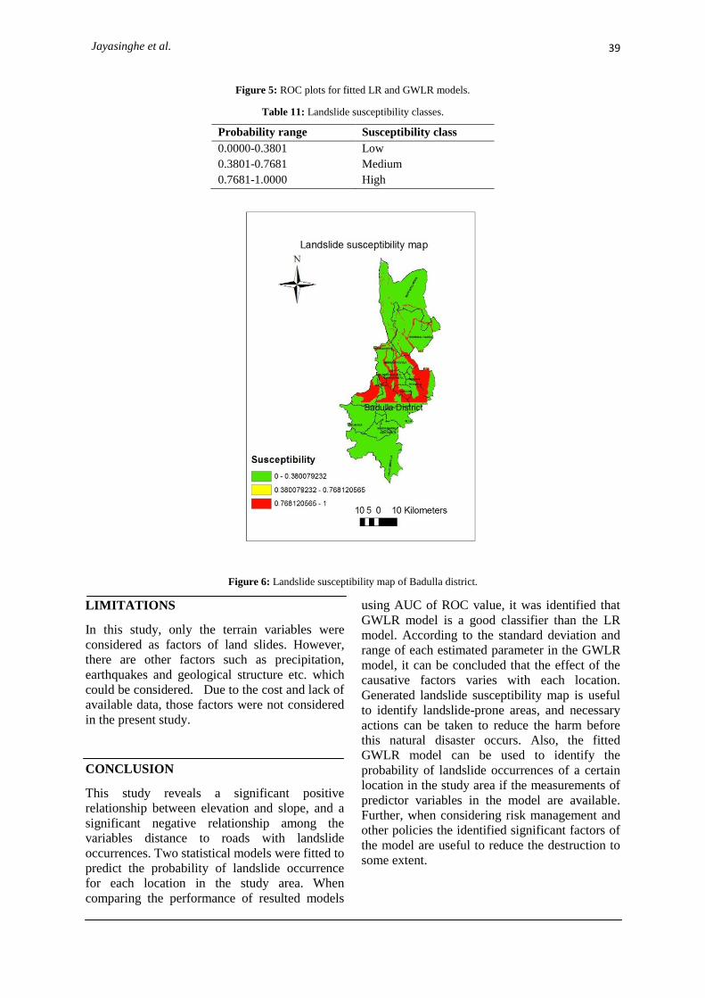
Generating landslide susceptibility map for
the study area
The probabilities of landslide occurrences (Y=1)
were obtained by using GWLR model for each
pixel in the study area, and these values were
then exported to the GIS software. Using the
standard deviation method (see statistical
methods section) available in the GIS, the
probabilities were used to classify the
susceptibility classes (low, medium, high). The
range of probabilities for each susceptibility class
is given in Table 11.
Finally, the landslide susceptibility map
(Figure 6) for Badulla district was drawn using
the susceptibility class of each pixel. According
to this map, it can be identified that certain areas
in Badulla, Uva Paranagama, Lunugala and Hali
Ela DS divisions are highly susceptible for
landslides.
Table 10: Test statistics for measuring Geographically variability.
Variable Test statistics
Elevation -14.65
Slope -10.55
Aspect -4.50
Plan curvature -2.02
Profile curvature 2.38
Distance to roads 6.00
Distance to streams 2.29
(a) (b)
39
Jayasinghe et al.
Figure 5: ROC plots for fitted LR and GWLR models.
Table 11: Landslide susceptibility classes.
Probability range Susceptibility class
0.0000-0.3801 Low
0.3801-0.7681 Medium
0.7681-1.0000 High
Figure 6: Landslide susceptibility map of Badulla district.
LIMITATIONS
In this study, only the terrain variables were
considered as factors of land slides. However,
there are other factors such as precipitation,
earthquakes and geological structure etc. which
could be considered. Due to the cost and lack of
available data, those factors were not considered
in the present study.
CONCLUSION
This study reveals a significant positive
relationship between elevation and slope, and a
significant negative relationship among the
variables distance to roads with landslide
occurrences. Two statistical models were fitted to
predict the probability of landslide occurrence
for each location in the study area. When
comparing the performance of resulted models
using AUC of ROC value, it was identified that
GWLR model is a good classifier than the LR
model. According to the standard deviation and
range of each estimated parameter in the GWLR
model, it can be concluded that the effect of the
causative factors varies with each location.
Generated landslide susceptibility map is useful
to identify landslide-prone areas, and necessary
actions can be taken to reduce the harm before
this natural disaster occurs. Also, the fitted
GWLR model can be used to identify the
probability of landslide occurrences of a certain
location in the study area if the measurements of
predictor variables in the model are available.
Further, when considering risk management and
other policies the identified significant factors of
the model are useful to reduce the destruction to
some extent.
40
Ceylon Journal of Science 46(4) 2017: 27-41
ACKNOWLEDGEMENTS
This work was supported through data provided
by National Building Resources Organization,
Institute of Surveying & Mapping, and National
Resource Management Centre, Sri Lanka.
REFERENCES
Brunsdon, C., Fotheringham, A. S., & Charlton, M.E.,
(1996). Geo-graphically weighted regression: A
method for exploring spatial non-stationarity.
Geographical Analysis 28(4), 281-298.
Courture, R., (2011). Landslides Terminology-
National Guidelines and Best Practices on
Landslides. Geological Survey of Canada p 12,
Open File 6824.
DeGraff, J., Romesburg, H., (1980). Regional
landslide susceptibility assessment for wildland
management: a matrix approach, In D. Coates &
J. Vitek (Eds.), Thresholds in Geomorphology
(pp. 401–414). George Allen and Unwin,
London.
Dieu, D. T., Pradhan, B., Lofman, O., &Revhaug, I.,
(2012). Landslide susceptibility Assessment in
Vietnam using Support vector machines,
Decision Tree, and Naive Bayes Models.
Mathematical problems in Engineering 2012: 1-
26. doi: 10.1155/2012/974638.
Disaster Mitigation in Asia and the Pacific (1991),
Collection of country reports, Asian
Development Bank, Manila, Philippines.
Esri (2015). „Standard deviation classification‟
[online] Available at:
http://support.esri.com/other-resources/gis-
ictionary/term/standard%20deviationclassificatio
n [Accessed 20 Jul. 2015]
Fotheringham, A.S., Brunsdon C., & Charlton, M.E.,
(2002). Geographically Weighted Regression:
The Analysis of Spatially Varying Relationships,
Wiley, Chichester.
Gorsevski, P. V., Gessler, P. E., Folt, R. B., & Elliot,
W. J., (2006). Spatial Prediction of landslide
hazard using logistic regression and ROC
analysis. Transactions in GIS, 10(3), 395-415.
Hoerl, A. E., & Kennard, R. W., (1971). Ridge
regression: biased estimates for nonorthogonal
problems. Technometrics 12: 55-67.
Lee, S., Digna, G., &Evangelist, (2005). Landslide
Susceptibility Mapping Using Probability and
Statistical Models in Baguio City, Philippines. In
Proceedings of 31stInternational Symposium on
Remote Sensing of Environment, June 20-24,
2005, Saint Petersburg, Russia.
Marston, R., Miller, M., & Devkota, L., (1998).
Geoecology and mass movements in the Manaslu
Ganesh &Langtang-JuralHimals, Nepal.
Geomorphology 26(1): 139–150.
Saefuddin, A., Setiabudi, A., &Fitrianto, A., (2012).
On comparison between Logistic Regression and
Weighted Logistic Regression: with Application
to Indonesia Poverty Data. World Applied
Sciences 19(2): 205-210. doi:
10.5829/idosi.wasj.2012.19.02.528.
Preethi, D., Sridhar, T.M. and Naidu C.V. (2011).
Carbohydrate concentration influences on in vitro
plant regeneration in Stevia rebaudiana. Journal
of Phytology 3(5): 61-64.
Rao, R.S., Ravishankar, G.A., 2002. Plant cell
cultures:chemical factories of secondary
metabolites. Biotechnology Advances 20: 101–
153.
Ramage, C.M. and Williams, R.R. (2002). Mineral
nutrition and plant morphogenesis. In Vitro
Cellular and Developmental Biology- Plant 38:
116-124.
Russo, A., Borrelli. F., 2005. Bacopa monniera, a
reputed nootropic plant: an overview.
Phytomedicine 12: 305-317.
Sarin, R. (2005). Useful metabolites from plant tissue
cultures. Biotechnology 4: 79–93.
Singh, H.K. and Dhawan, B.N. (1997).
Neurophychopharmacological effects of the
Ayurvedic nootropic Bacopa monniera Linn.
(Brahmi). Indian Journal of Pharmcology 29:
359-365.
Singh, H.K., Rastogi, R.P., Srimal, R.C. and Dhawan,
B.N. (1988). Effect of bacoside A and B on the
avoidance responses in rats. Phytotherapy
Research 2: 70-74.
Sivarajan, V.V. and Balachandran, I. (1994).
Ayurvedic Drugs and their Plant sources. Oxford
and IBH Publishing Co., New Delhi, pp. 97-99.
Srinivasan, V., Pestchanker, L., Moser, S., Hirasuna,
T.J., Taticek, R.A. and Shuler, M.L. (1995).
Taxol production in bioreactors: Kinetics of
biomass accumulation, nutrient uptake and taxol
production by cell suspension of Taxus baccata.
Biotechnology and Bioengineering 47: 666-676.
Tefera, W. and Wannakrairoj, S. (2004).
Micropropagation of Krawan (Amomum krervanh
Pierre ex Gagnep). Science Asia 30: 9-15.
Thompson, M. and Thorpe, T. (1987). Metabolic and
Non-metabolic Roles of Carbohydrates. In:
Bonga, J.M and Durzan, D.J., Ed. Cell and Tissue
Culture in Forestry. Martinus Nijhoff Publishers,
Dordrecht, pp. 89-112.
Tripathi, Y.B., Chaurasia, S., Tripathi, E., Upadhyaya,
A. and Dubey, G.P. (1996). Bacopa monniera
Linn. as an antitoxidant: mechanism of action.
Indian Journal of Experimental Biology 34, 523-
526.
Verpoorte, R., Contin, A. and Memelink, J. (2002).
Biotechnology for the production of plant
secondary metabolites. Phytochemistry Reviews
1, 13-25
Wu, C.H., Dewir, Y.H., Hahn, E.J. and Paek, K.Y.
(2006). Optimization of culturing conditions for
the production of biomass and phenolics from
adventitious roots of Echinacea angustifolia.
Journal of Plant Biology 49: 193-194.

41
Jayasinghe et al.
Weerasinghe, A., Puvenendran, S., Wickramasinghe,
A., Karunaratne, D. N., Wijesundara, S.
Karunaratne, V. (2013). Potent bioactivities of
the endemic Annonaceae heightens its dire
conservation status. Journal of the National
Science Foundation of Sri Lanka 41(4): 345-350.
Wermuth, C. G. (2003). The Practice of Medicinal
Chemistry. Amsterdam, the Netherlands:
Academic.
Youns, M., Hoheisel, J.D. and Efferth, T. (2010).
Toxicogenomics for the prediction of toxicity
related to herbs from traditional Chinese
medicine. Planta Medica 76: 2019-2025.
Zhong, G. S. and Wan, F. (1999). An outline on the
early pharmaceutical development before
Galen. Chinese Journal of Medical History 29:
178-182.

Recommended