Newton Method for theICA Mixture Model
Jason A. Palmer1 Scott Makeig1
Ken Kreutz-Delgado2 Bhaskar D. Rao2
1 Swartz Center for Computational Neuroscience2 Dept of Electrical and Computer EngineeringUniversity of California San Diego, La Jolla, CA
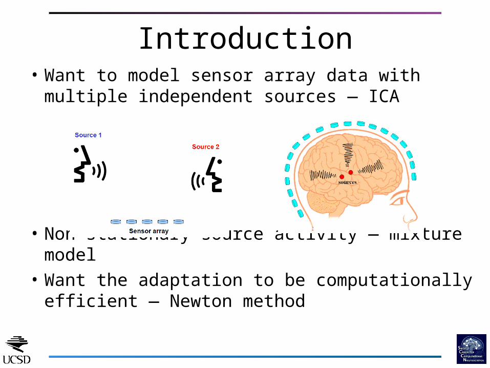
Introduction• Want to model sensor array data with multiple
independent sources — ICA
• Non-stationary source activity — mixture model• Want the adaptation to be computationally
efficient — Newton method
• ICA mixture model• Basic Newton method• Positive definiteness of Hessian when model
source densities are true source densities• Newton for ICA mixture model• Example applications to analysis of EEG
Outline
-10 -5 0 5 10
-10
-5
0
5
10
-10 -5 0 5 10
-10
-5
0
5
10
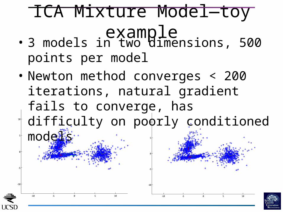
ICA Mixture Model—toy example• 3 models in two dimensions, 500 points per
model• Newton method converges < 200 iterations,
natural gradient fails to converge, has difficulty on poorly conditioned models
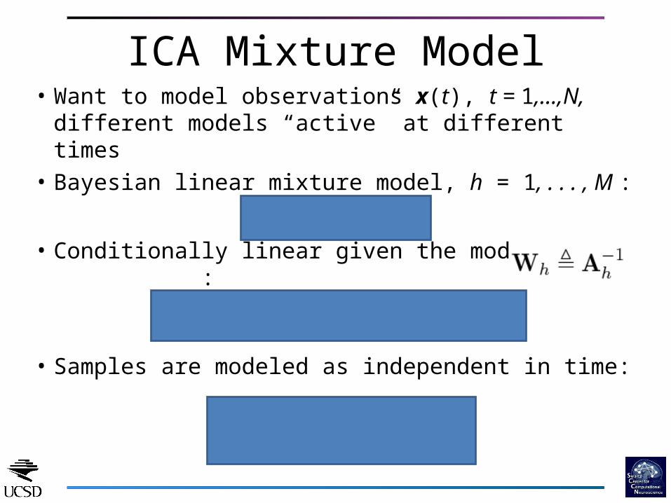
ICA Mixture Model• Want to model observations x(t), t = 1,…,N,
different models “active” at different times• Bayesian linear mixture model, h = 1, . . . , M :
• Conditionally linear given the model, :
• Samples are modeled as independent in time:
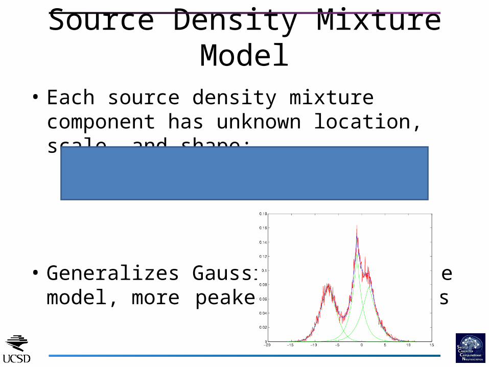
• Each source density mixture component has unknown location, scale, and shape:
• Generalizes Gaussian mixture model, more peaked, heavier tails
Source Density Mixture Model
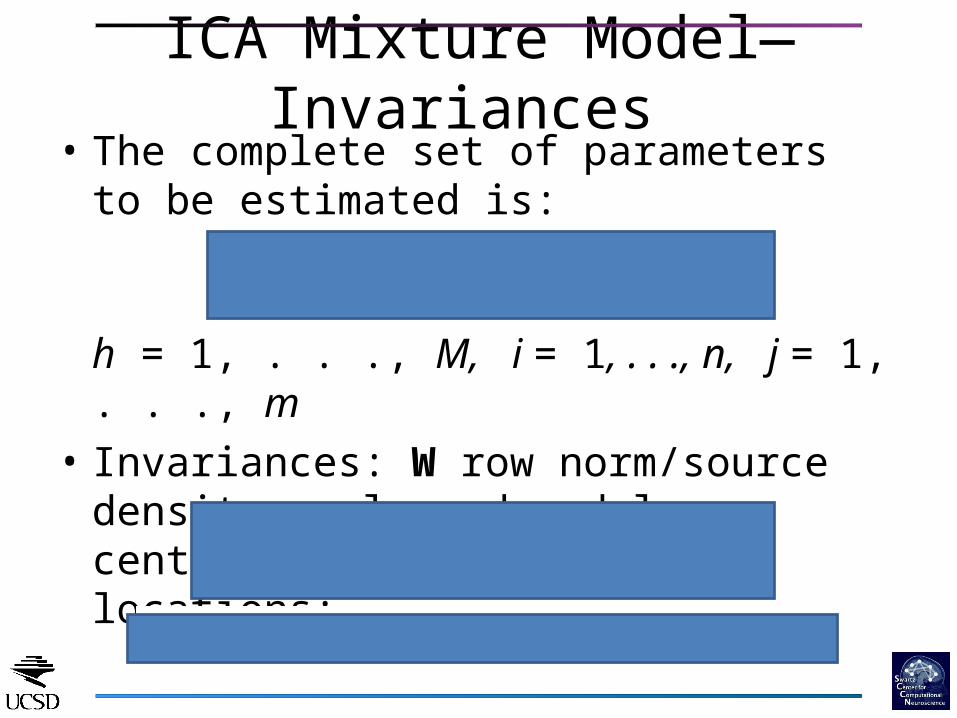
ICA Mixture Model—Invariances • The complete set of parameters to be
estimated is:
h = 1, . . ., M, i = 1, . . ., n, j = 1, . . ., m• Invariances: W row norm/source density scale
and model centers/source density locations:
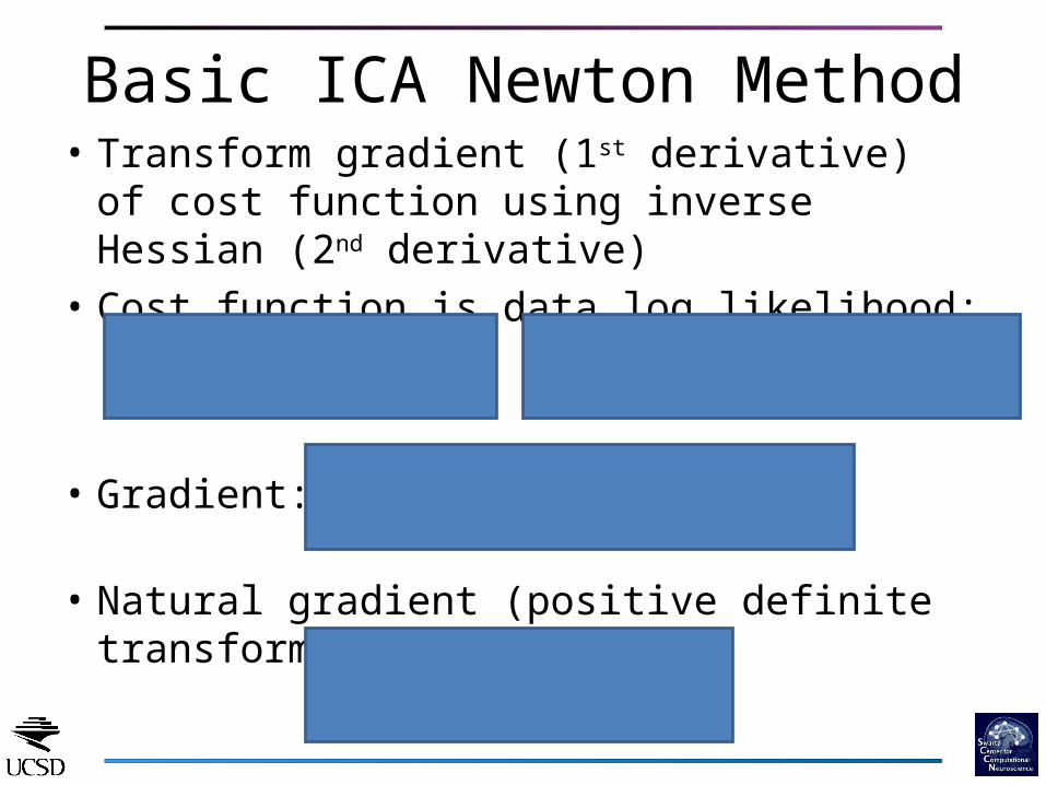
• Transform gradient (1st derivative) of cost function using inverse Hessian (2nd derivative)
• Cost function is data log likelihood:
• Gradient:
• Natural gradient (positive definite transform):
Basic ICA Newton Method

• Take derivative of (i,j)th element of gradient with respect to (k,l)th element of W :
• This defines a linear transform :
• In matrix form, this is:
Newton Method – Hessian
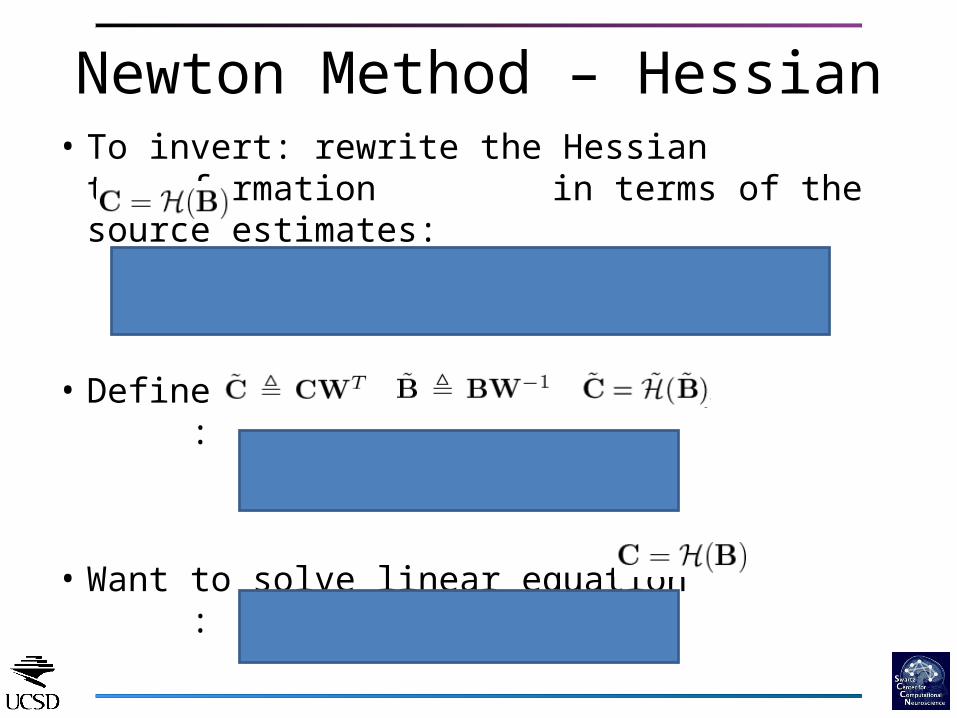
• To invert: rewrite the Hessian transformation in terms of the source estimates:
• Define , , :
• Want to solve linear equation :
Newton Method – Hessian

Newton Method – Hessian • The Hessian transformation can be simplified
using source independence and zero mean:
• This leads to 2x2 block diagonal form:
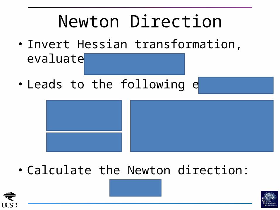
• Invert Hessian transformation, evaluate at gradient:
• Leads to the following equations:
• Calculate the Newton direction:
Newton Direction

Positive Definiteness of Hessian• Conditions for positive
definiteness: • Always true for true when model source
densities match true densities:1)
2)
3)
• Similar derivation applies to ICA mixture model:
Newton for ICA Mixture Model
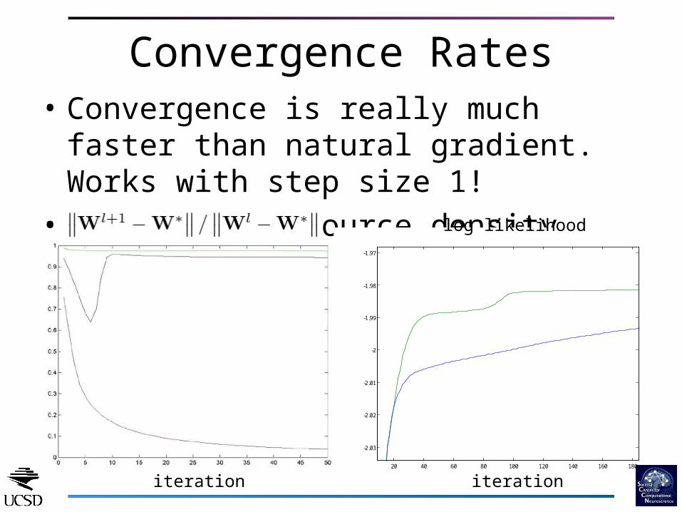
• Convergence is really much faster than natural gradient. Works with step size 1!
• Need correct source density model
20 40 60 80 100 120 140 160 180
-2.03
-2.02
-2.01
-2
-1.99
-1.98
-1.97
Convergence Rates
log likelihood
iterationiteration
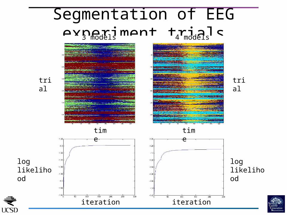
Segmentation of EEG experiment trials
trial trial
3 models 4 models
loglikelihood
loglikelihood
iteration iteration
time time

Applications to EEG—Epilepsy
time time
time
loglikelihood
loglikelihooddifferencefrom single model
1 model 5 models
Conclusion• We applied method of Amari, Cardoso and
Laheld, to formulate a Newton method for the ICA mixture model
• Arbitrary source densities modeled with non-gaussian source mixture model
• Non-stationarity modeled with ICA mixture model (multiple mixing matrices learned)
• It works! Newton method is substantially faster (superlinear). Also Newton can converge when Natural Gradient fails
Code• There is Matlab code available!!
– Generate toy mixture model data for testing– Full method implemented: mixture sources,
mixture ICA, Newton
• Extended version of paper in preparation, with derivation of mixture model Newton updates
• Download from:http://sccn.ucsd.edu/~jason
Acknowledgements
• Thanks to Scott Makeig, Howard Poizner, Julie Onton, Ruey-Song Hwang, Rey Ramirez, Diane Whitmer, and Allen Gruber for collecting and consulting on EEG data
• Thanks to Jerry Swartz for founding and providing ongoing support the Swartz Center for Computational Neuroscience
• Thanks for your attention!

Newton for ICA Mixture Model
Recommended