UNIVERSIDAD NACIONAL DE PIURA
FACULTAD DE ECONOMIA
DPTO. ACAD. DE ECONOMIA
SOLUCIÓN DEL EXAMEN PARCIAL DE ECONOMETRIA II
1º El investigador especifica el siguiente modelo:
���� � �� � ���� � ������� � � �� � ����� � ��
��� � �� � ����� � ���� � � �� � ���
�� � �� � ����� � ����� � � �� � � � Se le pide: 1.1. Realice la prueba de exogeneidad en la segunda ecuación. (3 puntos)
Dependent Variable: CAG
Method: Least Squares
Sample (adjusted): 1993 2005
Included observations: 13 after adjustments Variable Coefficient Std. Error t-Statistic Prob. C -12.03392 5.137579 -2.342333 0.0517
CAG(-1) 0.018494 0.407326 0.045404 0.9651
R 0.127466 0.078025 1.633658 0.1463
PAO 0.279729 0.095746 2.921558 0.0223
S(-1) 0.002159 0.005718 0.377661 0.7169
PP(-1) 0.001482 0.112167 0.013212 0.9898 R-squared 0.939464 Mean dependent var 1.910000
Modified: 1991 2005 // frcag.fit(f=na) cagf
1990 NA NA 1.508034 0.259962
1995 0.737793 0.702714 0.528168 0.616278 1.276703
2000 1.433483 1.525497 2.912789 3.998291 3.704256
2005 5.626031
Dependent Variable: S
Method: Least Squares
Sample (adjusted): 1993 2005
Included observations: 13 after adjustments Variable Coefficient Std. Error t-Statistic Prob. C -1036.393 454.3380 -2.281105 0.0565
CAG(-1) 46.66760 36.02157 1.295546 0.2362
R 13.96764 6.900062 2.024277 0.0826
PAO 20.35668 8.467269 2.404161 0.0472
S(-1) 0.132446 0.505647 0.261934 0.8009
PP(-1) -6.676478 9.919396 -0.673073 0.5225 R-squared 0.970661 Mean dependent var 194.7154
Modified: 1991 2005 // frs.fit(f=na) sf
1990 NA NA 3.805876 35.58787
1995 2.209473 44.75248 22.82673 37.49009 106.9751
2000 156.1114 210.5983 349.8195 473.6552 470.1401
2005 617.3277
Dependent Variable: PAG
Method: Least Squares
Sample (adjusted): 1993 2005
Included observations: 13 after adjustments Variable Coefficient Std. Error t-Statistic Prob. C 32.71483 5.745066 5.694422 0.0007
2
CAG 2.573000 1.868245 1.377228 0.2109
S -0.018198 0.021126 -0.861396 0.4175
R -0.374703 0.144690 -2.589697 0.0360
CAGF -1.302921 2.172942 -0.599611 0.5677
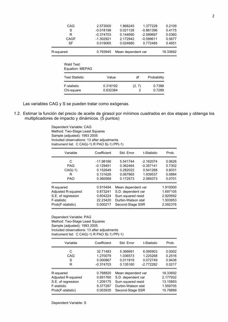
SF 0.019065 0.024680 0.772485 0.4651 R-squared 0.793945 Mean dependent var 18.33692
Wald Test:
Equation: MEPAG Test Statistic Value df Probability F-statistic 0.316192 (2, 7) 0.7388
Chi-square 0.632384 2 0.7289
Las variables CAG y S se pueden tratar como exógenas. 1.2. Estimar la función del precio de aceite de girasol por mínimos cuadrados en dos etapas y obtenga los
multiplicadores de impacto y dinámicos. (5 puntos)
Dependent Variable: CAG
Method: Two-Stage Least Squares
Sample (adjusted): 1993 2005
Included observations: 13 after adjustments
Instrument list: C CAG(-1) R PAO S(-1) PP(-1) Variable Coefficient Std. Error t-Statistic Prob. C -11.98166 5.541744 -2.162074 0.0626
PAG -0.129451 0.362464 -0.357141 0.7302
CAG(-1) 0.152649 0.282022 0.541268 0.6031
R 0.131626 0.067865 1.939537 0.0884
PAO 0.360569 0.172573 2.089373 0.0701 R-squared 0.915494 Mean dependent var 1.910000
Adjusted R-squared 0.873241 S.D. dependent var 1.697105
S.E. of regression 0.604224 Sum squared resid 2.920692
F-statistic 22.23420 Durbin-Watson stat 1.503953
Prob(F-statistic) 0.000217 Second-Stage SSR 2.092376
Dependent Variable: PAG
Method: Two-Stage Least Squares
Sample (adjusted): 1993 2005
Included observations: 13 after adjustments
Instrument list: C CAG(-1) R PAO S(-1) PP(-1) Variable Coefficient Std. Error t-Statistic Prob. C 32.71483 5.366691 6.095903 0.0002
CAG 1.270079 1.036573 1.225268 0.2516
S 0.000867 0.011919 0.072749 0.9436
R -0.374703 0.135160 -2.772282 0.0217 R-squared 0.768820 Mean dependent var 18.33692
Adjusted R-squared 0.691760 S.D. dependent var 2.177932
S.E. of regression 1.209175 Sum squared resid 13.15893
F-statistic 9.377287 Durbin-Watson stat 1.559705
Prob(F-statistic) 0.003935 Second-Stage SSR 15.78899
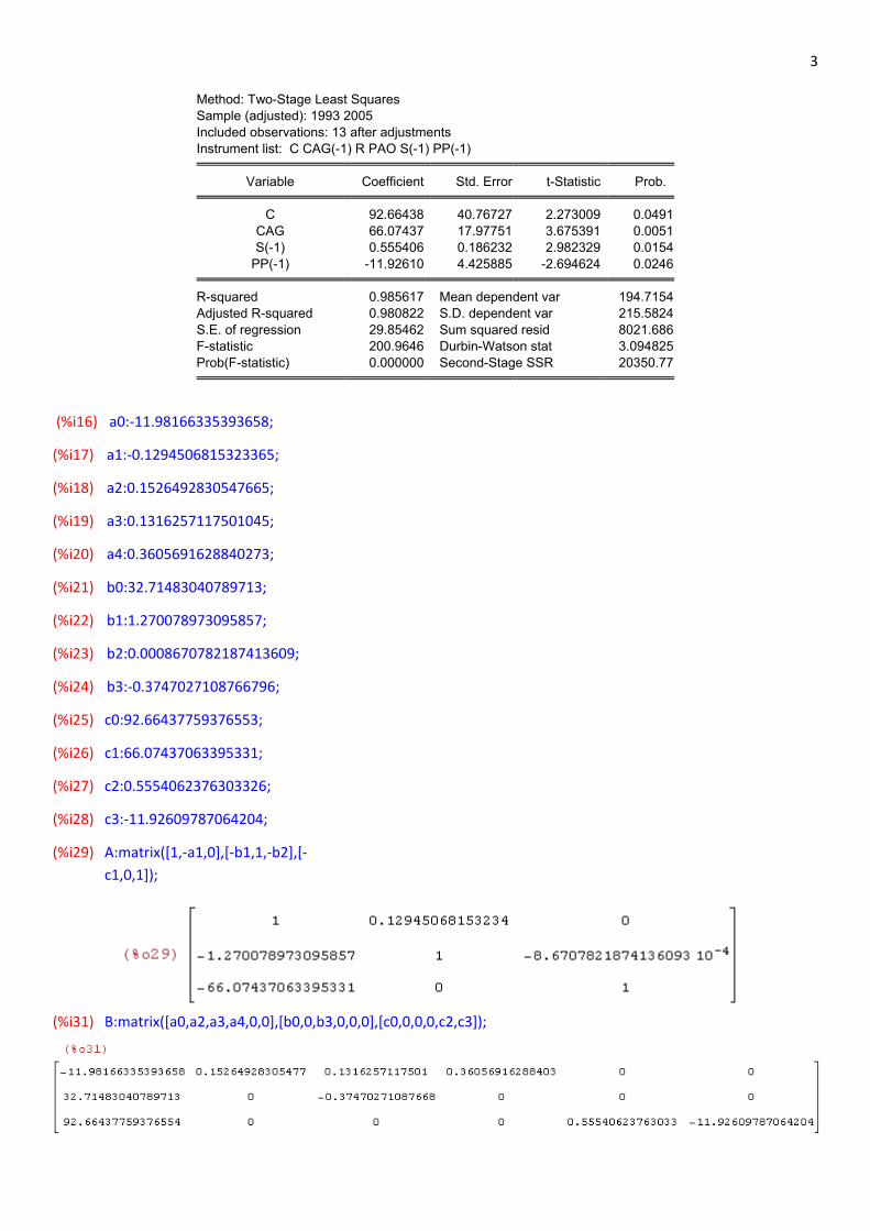
Dependent Variable: S
3
Method: Two-Stage Least Squares
Sample (adjusted): 1993 2005
Included observations: 13 after adjustments
Instrument list: C CAG(-1) R PAO S(-1) PP(-1) Variable Coefficient Std. Error t-Statistic Prob. C 92.66438 40.76727 2.273009 0.0491
CAG 66.07437 17.97751 3.675391 0.0051
S(-1) 0.555406 0.186232 2.982329 0.0154
PP(-1) -11.92610 4.425885 -2.694624 0.0246 R-squared 0.985617 Mean dependent var 194.7154
Adjusted R-squared 0.980822 S.D. dependent var 215.5824
S.E. of regression 29.85462 Sum squared resid 8021.686
F-statistic 200.9646 Durbin-Watson stat 3.094825
Prob(F-statistic) 0.000000 Second-Stage SSR 20350.77
(%i16) a0:-11.98166335393658;
(%i17) a1:-0.1294506815323365;
(%i18) a2:0.1526492830547665;
(%i19) a3:0.1316257117501045;
(%i20) a4:0.3605691628840273;
(%i21) b0:32.71483040789713;
(%i22) b1:1.270078973095857;
(%i23) b2:0.0008670782187413609;
(%i24) b3:-0.3747027108766796;
(%i25) c0:92.66437759376553;
(%i26) c1:66.07437063395331;
(%i27) c2:0.5554062376303326;
(%i28) c3:-11.92609787064204;
(%i29) A:matrix([1,-a1,0],[-b1,1,-b2],[-
c1,0,1]);
(%i31) B:matrix([a0,a2,a3,a4,0,0],[b0,0,b3,0,0,0],[c0,0,0,0,c2,c3]);
4
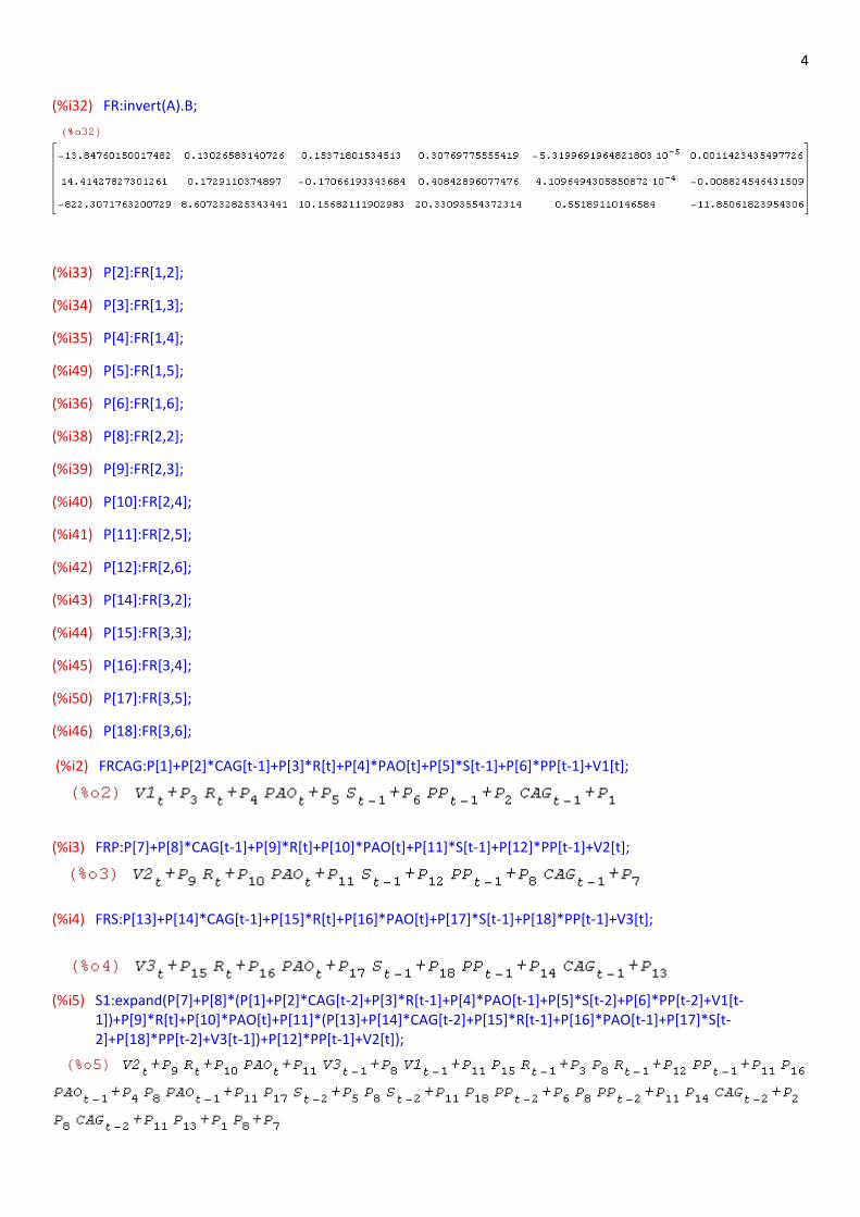
(%i32) FR:invert(A).B;
(%i33) P[2]:FR[1,2];
(%i34) P[3]:FR[1,3];
(%i35) P[4]:FR[1,4];
(%i49) P[5]:FR[1,5];
(%i36) P[6]:FR[1,6];
(%i38) P[8]:FR[2,2];
(%i39) P[9]:FR[2,3];
(%i40) P[10]:FR[2,4];
(%i41) P[11]:FR[2,5];
(%i42) P[12]:FR[2,6];
(%i43) P[14]:FR[3,2];
(%i44) P[15]:FR[3,3];
(%i45) P[16]:FR[3,4];
(%i50) P[17]:FR[3,5];
(%i46) P[18]:FR[3,6];
(%i2) FRCAG:P[1]+P[2]*CAG[t-1]+P[3]*R[t]+P[4]*PAO[t]+P[5]*S[t-1]+P[6]*PP[t-1]+V1[t];
(%i3) FRP:P[7]+P[8]*CAG[t-1]+P[9]*R[t]+P[10]*PAO[t]+P[11]*S[t-1]+P[12]*PP[t-1]+V2[t];
(%i4) FRS:P[13]+P[14]*CAG[t-1]+P[15]*R[t]+P[16]*PAO[t]+P[17]*S[t-1]+P[18]*PP[t-1]+V3[t];
(%i5) S1:expand(P[7]+P[8]*(P[1]+P[2]*CAG[t-2]+P[3]*R[t-1]+P[4]*PAO[t-1]+P[5]*S[t-2]+P[6]*PP[t-2]+V1[t-
1])+P[9]*R[t]+P[10]*PAO[t]+P[11]*(P[13]+P[14]*CAG[t-2]+P[15]*R[t-1]+P[16]*PAO[t-1]+P[17]*S[t-
2]+P[18]*PP[t-2]+V3[t-1])+P[12]*PP[t-1]+V2[t]);
5
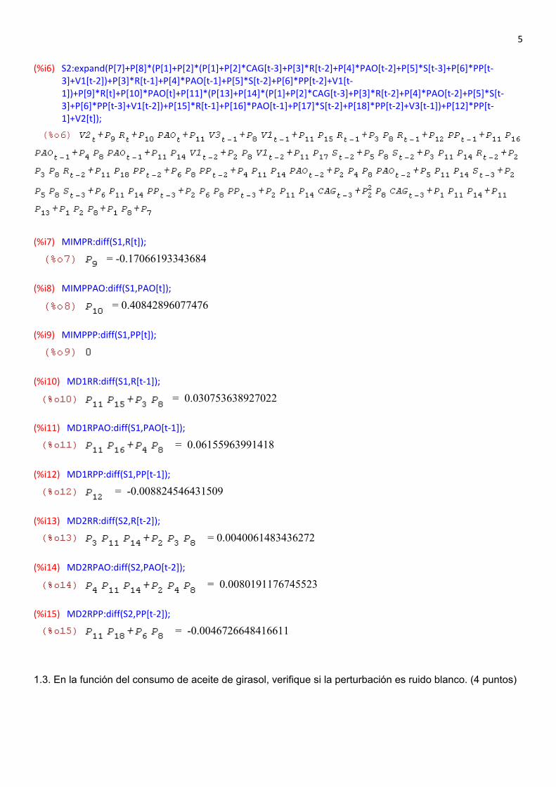
(%i6) S2:expand(P[7]+P[8]*(P[1]+P[2]*(P[1]+P[2]*CAG[t-3]+P[3]*R[t-2]+P[4]*PAO[t-2]+P[5]*S[t-3]+P[6]*PP[t-
3]+V1[t-2])+P[3]*R[t-1]+P[4]*PAO[t-1]+P[5]*S[t-2]+P[6]*PP[t-2]+V1[t-
1])+P[9]*R[t]+P[10]*PAO[t]+P[11]*(P[13]+P[14]*(P[1]+P[2]*CAG[t-3]+P[3]*R[t-2]+P[4]*PAO[t-2]+P[5]*S[t-
3]+P[6]*PP[t-3]+V1[t-2])+P[15]*R[t-1]+P[16]*PAO[t-1]+P[17]*S[t-2]+P[18]*PP[t-2]+V3[t-1])+P[12]*PP[t-
1]+V2[t]);
(%i7) MIMPR:diff(S1,R[t]);
= -0.17066193343684
(%i8) MIMPPAO:diff(S1,PAO[t]);
= 0.40842896077476
(%i9) MIMPPP:diff(S1,PP[t]);
(%i10) MD1RR:diff(S1,R[t-1]);
= 0.030753638927022
(%i11) MD1RPAO:diff(S1,PAO[t-1]);
= 0.06155963991418
(%i12) MD1RPP:diff(S1,PP[t-1]);
= -0.008824546431509
(%i13) MD2RR:diff(S2,R[t-2]);
= 0.0040061483436272
(%i14) MD2RPAO:diff(S2,PAO[t-2]);
= 0.0080191176745523
(%i15) MD2RPP:diff(S2,PP[t-2]);
= -0.0046726648416611
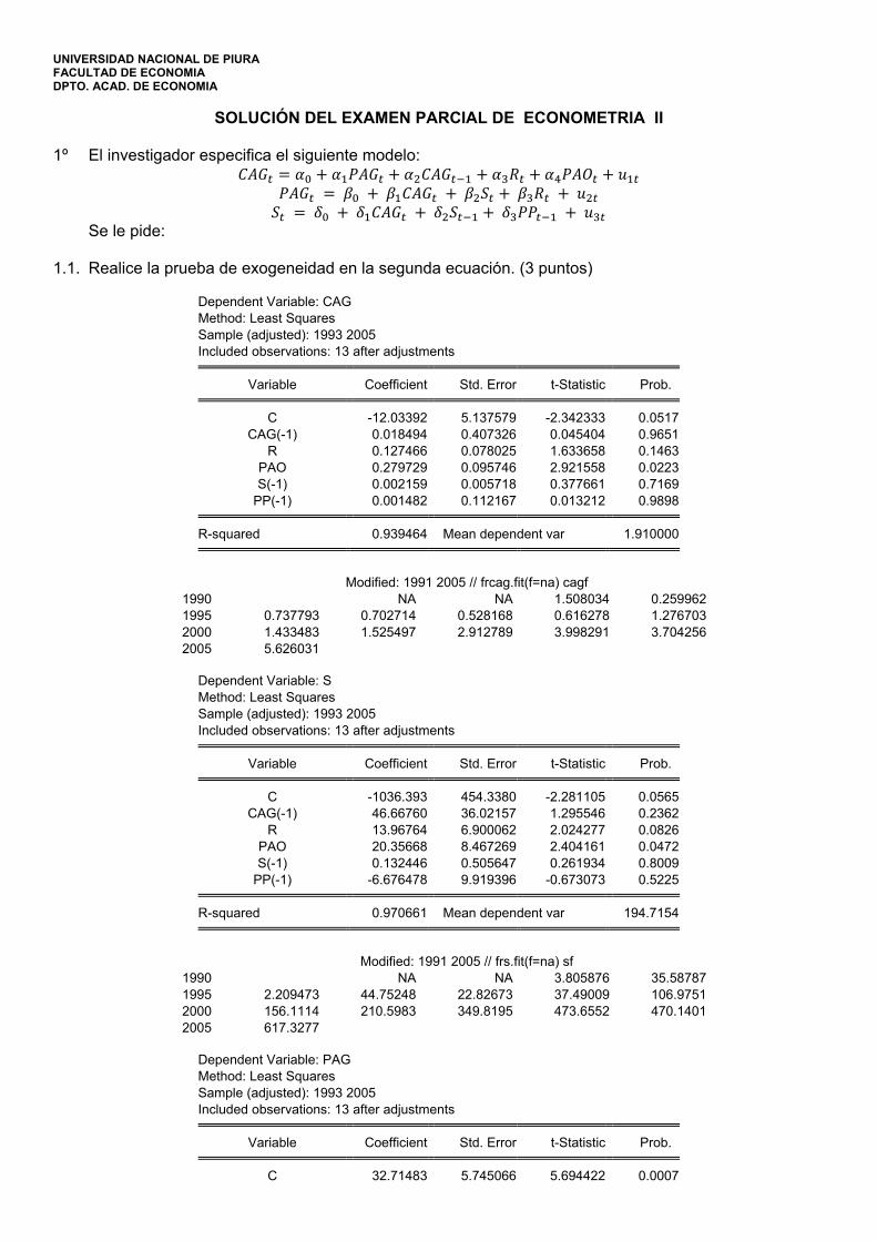
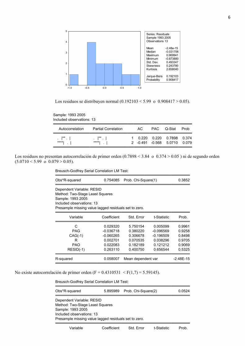
1.3. En la función del consumo de aceite de girasol, verifique si la perturbación es ruido blanco. (4 puntos)
6
0
1
2
3
4
5
-1.0 -0.5 0.0 0.5 1.0
Series: ResidualsSample 1993 2005
Observations 13
Mean -2.48e-15
Median -0.031706
Maximum 0.969941
Minimum -0.873880
Std. Dev. 0.493347
Skewness 0.243780
Kurtosis 2.658040
Jarque-Bera 0.192103
Probability 0.908417
Los residuos se distribuyen normal (0.192103 < 5.99 o 0.908417 > 0.05).
Sample: 1993 2005
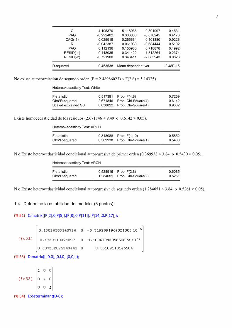
Included observations: 13 Autocorrelation Partial Correlation AC PAC Q-Stat Prob . |** . | . |** . | 1 0.220 0.220 0.7898 0.374
****| . | ****| . | 2 -0.491 -0.568 5.0710 0.079
Los residuos no presentan autocorrelación de primer orden (0.7898 < 3.84 o 0.374 > 0.05 ) ni de segundo orden
(5.0710 < 5.99 o 0.079 > 0.05).
Breusch-Godfrey Serial Correlation LM Test: Obs*R-squared 0.754085 Prob. Chi-Square(1) 0.3852 Dependent Variable: RESID
Method: Two-Stage Least Squares
Sample: 1993 2005
Included observations: 13
Presample missing value lagged residuals set to zero. Variable Coefficient Std. Error t-Statistic Prob. C 0.029320 5.750154 0.005099 0.9961
PAG -0.036718 0.380220 -0.096569 0.9258
CAG(-1) -0.060265 0.306678 -0.196509 0.8498
R 0.002701 0.070535 0.038296 0.9705
PAO 0.022083 0.182189 0.121212 0.9069
RESID(-1) 0.263110 0.400750 0.656544 0.5325 R-squared 0.058007 Mean dependent var -2.48E-15
No existe autocorrelación de primer orden (F = 0.4310531 < F(1,7) = 5.59145).
Breusch-Godfrey Serial Correlation LM Test: Obs*R-squared 5.895989 Prob. Chi-Square(2) 0.0524 Dependent Variable: RESID
Method: Two-Stage Least Squares
Sample: 1993 2005
Included observations: 13
Presample missing value lagged residuals set to zero. Variable Coefficient Std. Error t-Statistic Prob.
7
C 4.105370 5.118936 0.801997 0.4531
PAG -0.292402 0.336000 -0.870245 0.4176
CAG(-1) 0.025919 0.255664 0.101380 0.9226
R -0.042387 0.061930 -0.684444 0.5192
PAO 0.112136 0.155988 0.718878 0.4992
RESID(-1) 0.448035 0.341422 1.312264 0.2374
RESID(-2) -0.721900 0.346411 -2.083943 0.0823 R-squared 0.453538 Mean dependent var -2.48E-15
No existe autocorrelación de segundo orden (F = 2.48986023) < F(2,6) = 5.14325).
Heteroskedasticity Test: White F-statistic 0.517391 Prob. F(4,8) 0.7259
Obs*R-squared 2.671846 Prob. Chi-Square(4) 0.6142
Scaled explained SS 0.838822 Prob. Chi-Square(4) 0.9332
Existe homocedasticidad de los residuos (2.671846 < 9.49 o 0.6142 > 0.05).
Heteroskedasticity Test: ARCH F-statistic 0.318088 Prob. F(1,10) 0.5852
Obs*R-squared 0.369938 Prob. Chi-Square(1) 0.5430
N o Existe heterocedasticidad condicional autoregresiva de primer orden (0.369938 < 3.84 o 0.5430 > 0.05).
Heteroskedasticity Test: ARCH F-statistic 0.528916 Prob. F(2,8) 0.6085
Obs*R-squared 1.284651 Prob. Chi-Square(2) 0.5261
N o Existe heterocedasticidad condicional autoregresiva de segundo orden (1.284651 < 3.84 o 0.5261 > 0.05).
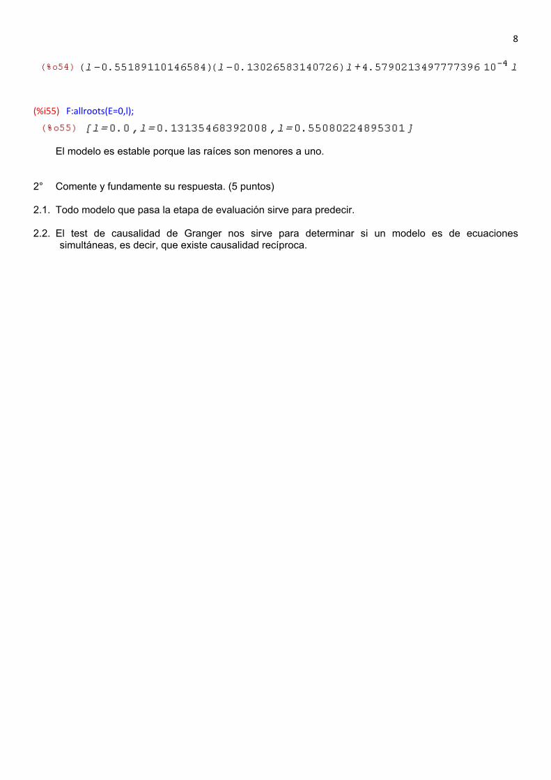
1.4. Determine la estabilidad del modelo. (3 puntos)
(%i51) C:matrix([P[2],0,P[5]],[P[8],0,P[11]],[P[14],0,P[17]]);
(%i53) D:matrix([l,0,0],[0,l,0],[0,0,l]);
(%i54) E:determinant(D-C);
8
(%i55) F:allroots(E=0,l);
El modelo es estable porque las raíces son menores a uno. 2° Comente y fundamente su respuesta. (5 puntos) 2.1. Todo modelo que pasa la etapa de evaluación sirve para predecir. 2.2. El test de causalidad de Granger nos sirve para determinar si un modelo es de ecuaciones
simultáneas, es decir, que existe causalidad recíproca.
Recommended