Numerical method for pricing american options under regime

Mathematical Theory and Modeling www.iiste.org

ISSN 2224-5804 (Paper) ISSN 2225-0522 (Online)

Vol.3, No.13, 2013

63

Numerical method for pricing American options under regime-

switching jump-diffusion models Abdelmajid El hajaji

Department of Mathematics, Faculty of Science and Technology,

University Sultan Moulay Slimane, Beni-Mellal, Morocco

E-mail: [email protected]

Khalid Hilal

Department of Mathematics, Faculty of Science and Technology,

University Sultan Moulay Slimane, Beni-Mellal, Morocco

E-mail: [email protected]

Abstract

Our concern in this paper is to solve the pricing problem for American options in a Markov-modulated jump-

diffusion model, based on a cubic spline collocation method. In this respect, we solve a set of coupled partial

integro-differential equations PIDEs with the free boundary feature by using the horizontal method of lines to

discretize the temporal variable and the spatial variable by means of Crank-Nicolson scheme and a cubic spline

collocation method, respectively. This method exhibits a second order of convergence in space, in time and also

has an acceptable speed in comparison with some existing methods. We will compare our results with some

recently proposed approaches.

Keywords: American Option, Regime-Switching, Crank-Nicolson scheme, Spline collocation, Free Boundary

Value Problem.

1. Introduction

Options form a very important and useful class of financial securities in the modern financial world. They play

a very significant role in the investment, financing and risk management activities of the finance and insurance

markets around the globe. In many major international financial centers, such as New York, London, Tokyo,

Hong Kong, and others, options are traded very actively and it is not surprising to see that the trading volume of

options often exceeds that of their underlying assets. A very important issue about options is how to determine

their values. This is an important problem from both theoretical and practical perspectives

Recently, there has been a considerable interest in applications of regime switching models driven by a Markov

chain to various financial problems. For an overview of Markov Chains

The Markovian regime-switching paradigm has become one of the prevailing models in mathematical finance.

It is now widely known that under the regime-switching model, the market is incomplete and so the option

valuation problem in this framework will be a challenging task of considerable importance for market

practitioners and academia. In an incomplete market, the payoffs of options might not be replicated perfectly by

portfolios of primitive assets. This makes the option valuation problem more difficult and challenging. Among

the many researchers that have addressed the option pricing problem under the regime-switching model, we must

mention the following: [4] develop a new numerical schemes for pricing American option with regime-switching.

[20] provides a general framework for pricing of perpetual American and real options in regime-switching Levy

models. [20] investigate the pricing of both European and American-style options when the price dynamics of

the underlying risky assets are governed by a Markov-modulated constant elasticity of variance process. [17]

develop a new tree method for pricing financial derivatives in a regimes-witching mean-reverting model. [22]

develop a flexible model to value longevity bonds under stochastic interest rate and mortality with regime-

switching.

The paper is organized as follows. In Section 2, we describe briefly the problem for American options in a

Markov-modulated jump-diffusion model. Then, we discuss time semi-discretization in Section 3. Section 4 is

devoted to the spline collocation method for pricing American options under regime-switching jump-diffusion

models using a cubic spline collocation method. Next, the error bound of the spline solution is analyzed. In order

to validate the theoretical results presented in this paper, we present numerical tests on three known examples in

Section 5. The obtained numerical results are compared to the ones given in [2]. Finally, a conclusion is given in

Section 6.



Vol.3, No.13, 2013

64

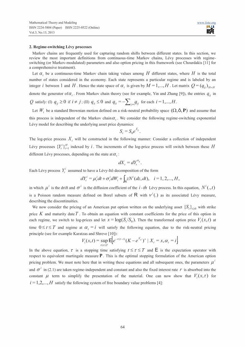
2. Regime-switching Lévy processes

Markov chains are frequently used for capturing random shifts between different states. In this section, we

review the most important definitions from continuous-time Markov chains, Lévy processes with regime-

switching (or Markov-modulated) parameters and also option pricing in this framework (see Chourdakis [11] for

a comprehensive treatment).

Let ta be a continuous-time Markov chain taking values among H different states, where H is the total

number of states considered in the economy. Each state represents a particular regime and is labeled by an

integer i between 1 and H . Hence the state space of ta is given by HM 1,...,= . Let matrix HHijqQ ´)(=

denote the generator of ta . From Markov chain theory (see for example, Yin and Zhang [9]), the entries ijq in

Q satisfy: (I) 0³ijq if ji ¹ ; (II) 0£iiq and ijijii qq å ¹-= for each .1,...,= Hi

Let tW be a standard Brownian motion defined on a risk-neutral probability space ),,( PôW and assume that

this process is independent of the Markov chain ta . We consider the following regime-switching exponential

Lévy model for describing the underlying asset price dynamics:

.= 0tX

t eSS

The log-price process tX will be constructed in the following manner: Consider a collection of independent

Lévy processes H

i

i

tY 1=}{ indexed by i . The increments of the log-price process will switch between these H

different Lévy processes, depending on the state at ta :

.= ttt dYdXa

Each Lévy process i

tY assumed to have a Lévy-Itô decomposition of the form

, 2,..., 1,= ),,(= HidtdzzNdWdtdY i

t

i

t

i

t

i

t ò++R

sm

in which im is the drift and

is is the diffusion coefficient of the i - th Lévy process. In this equation, )(.,tN i

is a Poisson random measure defined on Borel subsets of R with (.)in as its associated Lévy measure,

describing the discontinuities.

We now consider the pricing of an American put option written on the underlying asset 0}{ ³ttS with strike

price K and maturity dateT . To obtain an equation with constant coefficients for the price of this option in

each regime, we switch to log-prices and let )./(log= 0SSx t Then the transformed option price ),( txVi at

time Tt ££0 and regime at it =a will satisfy the following equation, due to the risk-neutral pricing

principle (see for example Karatzas and Shreve [10]):

[ ].= ,=|)( sup=),( )( ixXeKetxV tt

Xtr

Tti att

t

+--

££-E

In the above equation, t is a stopping time satisfying Tt ££t and E is the expectation operator with

respect to equivalent martingale measure P . This is the optimal stopping formulation of the American option

pricing problem. We must note here that in writing these equations and all subsequent ones, the parameters im

and is in (2.1) are taken regime-independent and constant and also the fixed interest rate r is absorbed into the

constant m term to simplify the presentation of the material. One can now show that ),( txVi for

Hi 1,2,...,= satisfy the following system of free boundary value problems [4]:



Vol.3, No.13, 2013

65

ïïïïï

î

ïïïïï

í

ì

-¶¶

-

-

£-

+-¶¶

®

®

+

å

,1,2,...,=,=)(

,1,2,...,=1,=lim

,1,2,...,=,=),(lim

,1,2,...,=,)(=),(

,1,2,...,=),(,=),(

,1,2,...,=),(>0,=

)(

)(

)(

1=

HiKTx

Hix

V

HieKxV

HieKTxV

HitxxeKxV

HixxVqVV

i

i

ixx

ix

iixx

x

i

ix

i

ijij

H

j

i

ii

t

t

tt

t

tt

L

(1)

in which )(tix for Hi 1,...,= denote the optimal exercise boundaries and i

L is the infinitesimal generator of

the i-th Lévy process of the form

),(),()()2

1(

2

1= 22 dzzxVVrVrVV i

ii

i

ix

i

ixxi

i ntlxlss +-++¶---¶- òRL

with

),(1)(=

,i stateat intensity jump for the stands

zdFez

i

-òRxl

for the function F which is the distribution of jumps sizes. This is a set of coupled partial integro-differential

equations with H free boundaries due to the regime-switching feature introduced in the underlying asset model.

The analytical solution of the above system of PIDEs is not available at hand and so the need for efficient

numerical approaches seems a necessity. In the sequel, we introduce our approach to solve this set of equations.

Remark: One should notice that if we set 0=l and 1=H ; (1) will become original Black-Scholes PDE.

3. Time and Spatial discretization

Our aim in this section is to use a cubic spline collocation method to find an approximate solution for the set of

Eqs. (1). By using the change of variables t-Tt = and applying the Crank-Nicolson scheme in time, we can

use the collocation method in each time step to find a continuous approximation in the whole interval. It is

obvious that ),( txVi for Hi 1,...,= satisfy the following set of coupled PIDEs in operator form:

,1,...,= 0,=1=

HiVqVt

Vjij

H

j

ii å-+

¶¶

L

which is valid in the space-time domain ][0,],[ T´+¥-¥ . In order to numerically approximate the solution, let

us truncate the x -domain into the sub domain ],[= maxminx xxW .

TakingT

HVVVV ],...,,[= 21 and ],,0[ Tx ´W=W

ïï

î

ïï

í

ì

Î

Î-

WÎ

WÎ-+¶¶

-¶¶

-¶¶

,],0[ ,0.=),(

,],0[ ,,0).(max=),(

,,.=,0)(

,),()),,((=)(2

2

TtItxV

TtIeKtxV

xIKxV

txtxVIVQGx

VR

x

VP

t

V

Hmax

H

x

min

xH (2)

where



Vol.3, No.13, 2013

66

( )( ) ,)(),()(=)(

,)(=

,)2

(=

,)2

(=

,][1,1,...,1=

1,...,=

1,...,=

1,...,=

2

1,...,=

,

2

dzzftzxVdiagVI

rdiagG

rdiagR

IdiagP

I

Hj

j

Hj

j

Hj

j

Hj

jj

HT

H

+

+

÷÷ø

öççè

æ--

÷÷ø

öççè

æÎ

òR

R

l

l

xls

s

with GQ- is a continuous, bounded, symmetric matrix function and each function of the matrix QG - is

0>~g³ on W and ,0)(max xeK - is sufficiently smooth function.

Here we assume that the problem satisfies sufficient regularity and compatibility conditions which guarantee that

the problem has a unique solution )()( 2,1 WÇWÎ CCV satisfying (see, [13, 1, and 14]):

4,030;),(

£+£££W£¶¶

¶ +

jiandjonktx

txVji

ji

(3)

where k is a constant in .HR

3.1. Time discretization and description of the Crank-Nicolson scheme

Discretize the time variable by setting tmtm D= for ,0,1,...,= Mm in which M

Tt =D and then define

),,(=)( mm txVxV

.0,1,...,= Mm

Now by applying the Crank-Nicolson scheme on (2), we arrive at the following equation

( ))()(2

1=)(

2

1)()( 111

mmmmmm

VIVIVVt

xVxV++-

D- ++

+

L

One way is to replace 1+mV with

mV in the linear terms. This leads to the following modified system:

).(2

=2

)( 11 mmmmm VtIVVt

Vt

xV D++DD

- ++LL (4)

For .0,1,...,= Mm The final price of the American option at time level m will be of the form:

ïïï

î

ïïï

í

ì

£

£

WÎ"

WÎ"+¶

¶+

¶¶

+

+

+++

.<0 ,0.=)(

,<0 ,.=)(

,,).(=)(

,),(=

1

1

0

0

11

2

12

MmIxV

MmIxV

xIxxV

xVJLVx

VR

x

VP

Hmax

m

Hmin

m

xH

x

mmmm

yf (5)

Where, for any 0³m and for any xx WÎ , we have



Vol.3, No.13, 2013

67

,=

,)(=)(

,)(=

),(22

=)(

,2

=

0

2

2

minx

x

mmmm

eK

eKx

IQGx

Rx

P

VIVt

VVJ

It

GQL

-

-

--¶¶

+¶¶

-D

-

÷ø

öçè

æD

--

+

yf

L

L

1+mV is solution of (5), at the 1)( +m th-time level.

The following theorem proves the order of convergence of the solution mV to .),( txV

Theorem 3.1 Problem (5) is second order convergent .i.e.

.)(),( 2tCVtxVH

m

m D£-

Proof: We introduce the notation m

mm VtxVe -),(= the error at step m and

|)(|maxsup=1

xee i

mHi

xx

Hm££WÎ

By Taylor series expansion of ,V we have

,).)((),(8

)(),(

2),(=),( 3

2

12

22

2

1

2

11 Hmmm

m ItOtxt

Vttx

t

VttxVtxV D+

¶¶D

+¶¶D

++++

+

.).)((),(8

)(),(

2),(=),( 3

2

12

22

2

1

2

1 Hmmm

m ItOtxt

Vttx

t

VttxVtxV D+

¶¶D

+¶¶D

-+++

By using these expansions, we get

,).)((),(=),(),( 2

2

11

Hm

mm ItOtxt

V

t

txVtxVD+

¶¶

D-

+

+ (6)

and by Taylor series expansion of t

V

¶¶

, we have

,).)((),(8

)(),(

2),(=),( 3

2

13

32

2

12

2

2

11 Hmmm

m ItOtxt

Vttx

t

Vttx

t

Vtx

t

VD+

¶¶D

+¶¶D

+¶¶

¶¶

++++

.).)((),(8

)(),(

2),(=),( 3

2

13

32

2

12

2

2

1 Hmmm

m ItOtxt

Vttx

t

Vttx

t

Vtx

t

VD+

¶¶D

+¶¶D

-¶¶

¶¶

+++

By using these expansions, and HIct

V.

3

3

£¶¶

on W (see relation (3)), we have

.).)((),(=)],(),([2

1 2

2

11 Hm

mm ItOtxVt

txVtxVt

D+¶¶

+¶¶

++

This implies

Hmmm

ItOtxVtxVt

txt

V).)(()],(),([

2

1=),( 2

1

2

1 D++¶¶

¶¶

++

.).)(())],((),()),((),([2

1= 2

11 Hmmmm ItOtxVItxVtxVItxV D++++ ++ LL

By using this relation in (6) we get



Vol.3, No.13, 2013

68

,).)(())],(()),(([2

),()2

(1=),()2

(1 3

11 Hmmmm ItOtxVItxVIt

txVt

txVt

D++D

+D

+D

- ++ LL

by (4). Then, we obtain

[ ] .).)(()()(2

)2

(1=)2

(1 3

11 Hmmmm ItOeIeIt

et

et

D++D

+D

+D

- ++ LL

We may bound the term ))(( 3tO D by 3)( tc D for some 0,>c and this upper bound is valid uniformly

throughout ][0,T . Therefore, it follows from the triangle inequality that

( ) .)()()(2

)2

()2

( 3

11 tceIeIt

et

Iet

IHmHm

H

m

H

m D++D

+D

+£D

- ++ LL

We use the cross-correlation function (see [3]) defined by

,1,...,=,)()(=)(**)(=)( HifordzzxezfxexfxR i

m

i

mimfe

+òR

we have

.HmHHm

fe efR £

( ) ,)()()(2

)2

()2

( 3

11 tceIeIt

et

Iet

IHmHm

H

m

H

m D++D

+D

+£D

- ++ LL

( ) .)(2

)2

( 3

1 tceeft

et

IHmHmHHHm

H

D++D

+D

+£ +lL

Clearly, the operator ÷ø

öçè

æ D± L

2

tIH satisfies a maximum principle (see, [7, 5]) and consequently

.~

21

1

2

1

÷÷÷÷÷

ø

ö

ççççç

è

æ

D+

£÷ø

öçè

æ D±

-

gt

tI

H

H L

Since we are ultimately interested in letting 0®Dt , there is no harm in assuming that 2<.htD , with

( )HHH

flh +L= . We can thus deduce that

.)(

.2

11.

2

11

.2

11

3

1 t

t

ce

t

t

eHmHm D

÷÷÷÷

ø

ö

çççç

è

æ

D-+

÷÷÷÷

ø

ö

çççç

è

æ

D-

D+£+

hh

h (7)

We now claim that

.)(1

.2

11

.2

11

2t

t

tc

e

m

Hm D

úúúú

û

ù

êêêê

ë

é

-÷÷÷÷

ø

ö

çççç

è

æ

D-

D+£

h

h

h (8)

The proof is by induction on m . When 0=m we need to prove that 00 £H

e and hence that 0=0e . This

is certainly true, since at 0=0t the numerical solution matches the initial condition and the error is zero.

For general 0³m , we assume that (8) is true up to m and use (7) to argue that



Vol.3, No.13, 2013

69

32

1 )(

.2

11

)(1

.2

11

.2

11

.2

11

.2

11

t

t

ct

t

t

t

tc

e

m

Hm D÷÷÷÷

ø

ö

çççç

è

æ

D-+D

úúúú

û

ù

êêêê

ë

é

-÷÷÷÷

ø

ö

çççç

è

æ

D-

D+

÷÷÷÷

ø

ö

çççç

è

æ

D-

D+£+

hh

h

h

h

h

.)(1

.2

11

.2

11

2

1

t

t

tc

m

D

úúúú

û

ù

êêêê

ë

é

-÷÷÷÷

ø

ö

çççç

è

æ

D-

D+£

+

h

h

h

This advances the inductive argument from m to 1+m and proves that (8) is true. Since 2,<.<0 htD it is

true that

.

.2

11

.=

.2

11

.

!

1

.2

11

.1=

.2

11

.2

11

0= ÷÷÷÷

ø

ö

çççç

è

æ

D-

D

÷÷÷÷

ø

ö

çççç

è

æ

D-

D£÷÷÷÷

ø

ö

çççç

è

æ

D-

D+

÷÷÷÷

ø

ö

çççç

è

æ

D-

D+å¥

h

h

h

h

h

h

h

h

t

texp

t

t

lt

t

t

t

l

l

Consequently, relation (8) yields

.

.2

11

.)(

.2

11

.2

11

)( 22

÷÷÷÷

ø

ö

çççç

è

æ

D-

DD£

÷÷÷÷

ø

ö

çççç

è

æ

D-

D+D£

h

hhh

h

ht

tmexp

tc

t

ttc

e

m

Hm

This bound is true for every nonnegative integer m such that Ttm <D . Therefore

.

.2

11

.)( 2

÷÷÷÷

ø

ö

çççç

è

æ

D-

D£

h

hh

t

Texp

tce

Hm

We deduce that

.)(),( 2tCVtxVH

m

m D£-

In other words, problem (5) is second order convergent.

For any 0³m , problem (5) has a unique solution and can be written on the following form:

ïï

î

ïï

í

ìWÎ"Î+¢+¢¢

0,=)(

,.=)(

,,)(~

=)()()(

max

Hmin

x

H

xV

IxV

xxfxLVxVRxVP

yR

(9)

In the sequel of this paper, we will focus on the solution of problem (9).

3.2. Spatial discretization and cubic spline collocation method

Let Ä denotes the notation of Kronecker product, . the Euclidean norm on Hn ++1

R and )(kS the

thk

derivative of a function S .

In this section we construct a cubic spline which approximates the solution V of problem (9), in the

interval RÌWx .

Let }====<<<<===={= 321110123 maxnnnnnmin xxxxxxxxxxxx +++----Q L be a

subdivision of the interval xW . Without loss of generality, we put ihaxi += , where ni ££0



Vol.3, No.13, 2013

70

andn

xxh minmax -= . Denote by ),(=),( 2

34 QWQW xx PS the space of piecewise polynomials of degree less

than or equal to 3 over the subdivisionQ and of class2C everywhere on xW . Let ,iB 1,3,= -- ni L , be the

B-splines of degree 3 associated with .Q These B-splines are positives and form a basis of the

space .),(4 QWxS

Consider the local linear operator 3Q which maps the function V onto a cubic spline space ),(4 QWxS and

which has an optimal approximation order. This operator is the discrete 2C cubic quasi-interpolant (see [15])

defined by

,)(=1

3=

3 ii

n

i

BVVQ må-

-

where the coefficients )(Vjm are determined by solving a linear system of equations given by the exactness of

3Q on the space of cubic polynomial functions .)(3 xWP Precisely, these coefficients are defined as follows:

ïïïï

î

ïïïï

í

ì

++-

---+-

+-+

-

----

+++

-

-

).(=)(=)(

)),(7)(18)(9)((218

1=)(

3,1,...,=for )),()(8)((6

1=)(

)),(2)(9)(18)((718

1=)(

),(=)(=)(

1

1232

321

32102

03

maxnn

nnnnn

jjjj

min

xVxVV

xVxVxVxVV

njxVxVxVV

xVxVxVxVV

xVxVV

m

m

m

m

m

It is well known (see e.g. [16], chapter 5) that there exist constants kC , 0,1,2,3,=k such that, for any

function )(4

xCV WÎ ,

0,1,2,3,= ,)(44)(

3

)( kVhCVQVH

kk

kH

kk --£- (10)

By using the boundary conditions of problem (9), we obtain Hminmin IxVxVQV .=)(=)(=)( 33 ym-

and .0.=)(=)(=)( 31 Hmaxmaxn IxVxVQV-m Hence

,= 13 SzVQ +

where

.)(,,)(==2

2=

1

2

2=

31

T

jHj

n

j

jj

n

j

H BVBVSandIBz úû

ùêë

éåå-

-

-

-- mmy L

From equation: (10), we can easily see that the spline S satisfies the following equation

njIhOxgxLSxRSxPS Hjjjj 0,...,= ,).()(=)()()( 2(0)(1)(2) +++ (11)

with

.0,...,= ,))()()(()(~

=)( (0)

1

(1)

1

(2)

1 njxLzxRzxPzxfxg H

jjjjj RÎ++-

The goal of this section is to compute a cubic spline collocation jij

n

ji BcSp ,

1

3=

~=

~

å -

-, Hi 1,...,= which

satisfies the equation (9) at the points jt , 20,...,= +nj with 00 = xt , 2

=1 jj

j

xx +-t , nj ,1,= L ,

11 = -+ nn xt and nn x=2+t .

Then, it is easy to see that



Vol.3, No.13, 2013

71

.1,...,=0,=~

=~

1,3, Hiforcandc ini -- y

Hence

HiforBcSwhereSzSp jij

n

j

iii1,...,=,

~=

~ ,

~=

~,

2

2=

1 å-

-

+

and the coefficients ijc ,

~, 22,...,= -- nj and Hi 1,...,= satisfy the following collocation conditions:

1,1,...,= ),(=)(~

)(~

)(~

(0)(1)(2)

+++ njgSLSRSP jjjj tttt (12)

where

1.1,...,= ,))()()(()(~

=)(

,]~

,...,~

[=~

(0)

1

(1)

1

(2)

1

1

+Î++- njLzRzPzfg

SSS

H

jjjjj

TH

Rttttt

Taking

[ ]

,~

,...,~

,...,~

,...,~

=~

,)(),...,(),...,(),...,(=

12,2,2,12,1

1

221212

Hn

T

HnHn

HnT

HnHn

ccccC

VVVVC

++----

++----

Îúúû

ù

êêë

é

Î

R

Rmmmm

and using equations (11) and (12), we get:

( ) EFCALARAP hhh +Ä+Ä+Ä =)()()( (0)(1)(2) (13)

and

( ) ,=~

)()()( (0)(1)(2) FCALARAP hhh Ä+Ä+Ä (14)

with

0,1,2,= ,))((=

,)](),...,([=

,)(1

= and],...,[=

1,1

)(

3

)(

122

11

kBAt

hO

t

hOE

gt

gggF

npjj

k

p

k

h

HnT

H

jj

T

n

+££+-

++

+

ÎDD

ÎD

t

t

R

R

It is well known that kk

k

h Ah

A1

=)( for 0,1,2=k where matrices 0A , 1A and 2A are independent of h , with

the matrix 2A is invertible [8].

Then, relations (13) and (14) can be written in the following form

( ) ,=)( 22

2 EhFhCVUIAP +++Ä (15)

( ) ,=~

)( ~

2

2C

FhCVUIAP ++Ä (16)

with

),()(= 1

1

2 ARAPhU ÄÄ -

(17)

).()(= 0

1

2

2 ALAPhV ÄÄ -

(18)

In order to determine the bounded of ¥- ||~

|| CC , we need the following Lemma.



Vol.3, No.13, 2013

72

Lemma 3.1 If 4

<2 th

Dr , then VUI ++ is invertible, where .||)(||= 1

2 ¥-Ä APr

Proof: From the relation (17), we have

¥¥-

¥ ÄÄ£ ||)(||||)(|||||| 1

1

2 ARAPhU

.||)(|| 1 ¥Ä£ ARhr

For h sufficiently small, we conclude

.4

1<|||| ¥U (19)

From the relation (18) and 1|||| 0 £¥A , we have

¥¥-

¥ ÄÄ£ ||||||)(|||||| 0

1

2

2 ALAPhV

¥¥-Ä£ ||||||)(|| 1

2

2 LAPh

÷ø

öçè

æD

+-£ ¥t

GQh2

||||2r

.2

||||2

2

t

hGQh

D+-£ ¥

rr

For h sufficiently small, we conclude that4

1<||||2

¥-GQh r . Then

.2

4

1<||||

2

t

hGQ

D+- ¥

r (20)

As .2

1<

2 2

t

h

Dr

So, ,1<|||||||| |||| VUVU +£+ and therefore VUI ++ is invertible.

Proposition 3.1 If r4

2 th

D£ , then there exists a constant cte which depends only on the functions ,p q , l

and g such that

..||~

|| 2hcteCC £- (21)

Proof: Assume that .4

2

rt

hD

£ From (15) and (16), we have

.)()(=~

1

2

12 EAPVUIhCC -- Ä++-

Since ,)(=2

t

hOED

then there exists a constant 1K such that .||||2

1t

hKED

£ This implies that

||||||)(||||)(||||~

|| 1

2

12 EAPVUIhCC ¥-

¥- Ä++£-

2

1

12

||)(|| hKVUIt

h¥

-++D

£r

.||)(||4

1 2

1

1 hKVUI ¥-++£

On the other hand, from (19) and (20), we get .1<|||| ¥+VU Thus



Vol.3, No.13, 2013

73

.=||||1

1||)(|| 1 cte

VUVUI

¥¥

-

+-£++

Finally, we deduce that

..||~

|| 2hcteCC £-

Now, we are in position to prove the main theorem of our work.

Proposition 3.2 The spline approximation

~Sp converges quadratically to the exact solution V of problem (2),

i.e., )(=~

2hOSpV

H

- .

Proof: From the relation (10), we have

)(=)( 4

3 hOVQVH

- , so ,)( 4

3 KhVQVH£- where K is a positive constant. On the other

hand we have

.1,...,=),()~

)((=)(~

))(( ,

2

2=

3 HiforxBcVxSpxVQ jijij

n

j

ii -- å-

-

m

Therefore, by using (21) and 1)(2

2=£å

-

-xB j

n

j, we get

.1,...,=,||~

||)(||~

|||)(~

))((| 2

1

2

2=

3 HiforhKCCxBCCxSpxVQ j

n

j

ii £-£-£- å-

-

Since ,||~

)(||||)(||||~

)(|| 333 HHH SpVQVQVSpVQ -+-£- we deduce the stated result.

4. Numerical examples

In this section we verify experimentally theoretical results obtained in the previous section. If the exact

solution is known, then at time Tt £ the maximum error maxE can be calculated as:

.|),(),(|max= ,

],1[0,],,[

txVtxSE i

NM

iHiTt

maxx

minxx

max -££ÎÎ

Otherwise it can be estimated by the following double mesh principle:

,|),(),(|max= ,22,

],1[0,],,[, txStxSE NM

i

NM

iHiTt

maxx

minxx

max

NM -££ÎÎ

where ),(, txS NM

i is the numerical solution on the 1+M grids in space and 1+N grids in time, and

),(,22 txS NM

i is the numerical solution on the 12 +M grids in space and 12 +N grids in time, for

Hi ££1 .

We need to estimate the integral dzzxV im

i n)( +òR and for this purpose we use a Gaussian quadrature

formula in a bounded interval of the form ],[ maxmin zz to arrive at

,)()()()()(1=

kk

m

ik

p

k

im

i

maxz

minz

iim

i zfzxVwdzzfzxVdzzxV +»+»+ åòò llnR

(22)

for Hi 1,..,= in which the kw ’s are the Gaussian quadrature coefficients; cf. [21, 6] for details.

We present two examples to better illustrate the use of the switching Lévy approach and the proposed pricing

methodology in concrete situations. These examples are concerned with American put options in three and five

world states respectively. In the first example, we assume that the stock price follows a Merton jump-diffusion

process with an intensity parameter governed by a three-state hidden Markov chain. In the second one, we

consider the Kou jump diffusion model with jump intensities having a discrete five-state Markov dynamics.

4.1. Example 1



Vol.3, No.13, 2013

74

In this example, we assume a three-regime economy in which the dynamics of the underlying stock price in the

i-th regime obeys a Merton jump-diffusion process with the Lévy measure

},2

)({

2=)(

2

2

j

j

j

ii

zexpz

s

m

spl

n-

-

where the intensity vector is given by: ,.7][0.3,0.5,0= Tl

the generator matrix is defined by

and the a priori state probabilities are given to be ..5][0.2,0.3,0= Tp

Other useful data are provided in the following table:

Table 1. Data used to value American options under regime-switching jump-diffusion models.

Parameter values

S 100

K 100

T 1

s 0.15

r 0.05

js 0.45

jm 0.5-

For this problem, we use a uniform distribution of points in the interval 6,6][=],[ maxmin -xx for the

collocation process and truncate the integration domain in (22) according to

,/2))2(log2(= 2

max jjjz mpess +-

,= maxmin zz -

with .10= 12-ee We must note here that using these two bounds forces the total truncation error to be

uniformly bounded by e and the derivation of them is described in full detail in [12] and [19].

The comparison of the maximum error values between the method developed in this paper with the one

developed in [2] will be taken at five different values of the number of space steps

2048, 1024, 512, 256,=N and time steps 1024, 512, 256, 128,=M .

We conduct experiments on different values of N , M ands . Table 2 show values of the maximum error

(max_error) obtained in our numerical experiments and the one obtained in [2]. We see that the values of

maximum error obtained by our method improve the ones in [2].

Table 2. Numerical results for three world states

N M Our max_error max_error in [2]

256 128 3100.83 -´

3102.86 -´

512 256 3100.20 -´

3101.78 -´

1024 512 4100.52 -´

3100.88 -´

2048 1024 4100.13 -´

3100.36 -´

4.2. Example 2

In this example, we assume that the stock price process follows the Kou jump-diffusion model where the

jumps arrive at Poisson times and are distributed according to the law

).1)(11(=)( 0<

220

11 z

z

z

zii epepzhh hhln -+³

-

.

4.03.01.0

8.012.0

2.06.08.0

=

úúú

û

ù

êêê

ë

é

-

-

-

Q



Vol.3, No.13, 2013

75

We assume that our five-state Markov chain has a generator of the form:

,

125.025.025.025.0

25.0125.025.025.0

25.025.0125.025.0

25.025.025.0125.0

25.025.025.025.01

=

úúúúúú

û

ù

êêêêêê

ë

é

-

-

-

-

-

Q

and that the economy switches between different jump intensities described by the vector

.].5,0.7,0.9[0.1,0.3,0= Tl

In this case, we suppose that the market could be in any of the five regimes with equal probability. Other

corresponding information is given in the following table:

Table 3. Data used to value American options under regime-switching jump-diffusion models.

Parameter values

S 100

K 100

T 0.25

s 0.5

r 0.05

p 0.5

1h 3

2h 2

We use a uniform distribution of points in the interval 6,6][=],[ maxmin -xx as collocation points and use the

following bounds for the truncation process in (22):

),)/(1/(log= 1max he -pz

)))/(1/(1(log= 2min he --- pz,

where we use the value of 1210= -ee . We refer the reader to [19] to see a full derivation of these bounds in

order to obtain uniform truncation error bounds. Table 3 contains the option prices corresponding to each

intensity regime reported for different values of N andM .

The comparison of the maximum error values between the method developed in this paper with the one

developed in [2] will be taken at five different values of the number of space steps 8198 1024, 512,=N and

time steps 512 512, 256,=M for ,0.1=1l ,0.3=2l ,0.5=3l 0.7=4l and 0.9=5l .

We conduct experiments on different values of ,N M and .l Table 4 show values of the maximum error

(max_error) obtained in our numerical experiments and the one obtained in [2]. We see that the values of

maximum error obtained by our method improve the ones in [2].

5. Conclusion

In this paper, a cubic spline collocation approach is introduced to price American options in a regime-switching

Lévy context. After a brief review of the process of deriving the set of coupled PIDEs describing the prices in

different regimes, we present the details of our methodology which consists of first discretizing in time (by

Crank-Nicolson scheme) and then collocating in space (by a cubic spline ollocation method). Then, we have

shown provided an error estimate of order )( 2hO with respect to the maximum norm .H

In our paper we

consider a cubic spline space defined by multiple knots in the boundary and we propose a simple and efficient

new collocation method by considering as collocation points the mid-points of the knots of the cubic spline space.

It is observed that the collocation method developed in this paper, when applied to some examples, can improve

the results obtained by the collocation methods given in the literature. The two test problems which are studied



Vol.3, No.13, 2013

76

in this paper demonstrate that this approach has an efficient alternative to the one proposed in [2].

Table 4. Numerical results for different intensity regimes and discretization parameters.

N M Our max_error max_error in [2]

For 0.1=1l

512 256 0.00150 0.0356

1024 512 0.00037 0.0132

8198 512 0.00030 0.0060

For 0.3=2l

512 256 0.00146 0.0348

1024 512 0.00036 0.0136

8198 512 0.00029 0.0066

For 0.5=3l

512 256 0.00143 0.0341

1024 512 0.00035 0.0138

8198 512 0.00028 0.0070

For 0.7=4l

512 256 0.00139 0.0339

1024 512 0.00034 0.0140

8198 512 0.00027 0.0071

For 0.9=5l

512 256 0.00133 0.0338

1024 512 0.00033 0.0142

8198 512 0.00026 0.0072

Acknowledgment

We are grateful to the reviewers for their constructive comments that helped to improve the paper.

References

[1] A. Friedman. (1983). Partial Differential Equation of Parabolic Type, Robert E. Krieger Publiching Co.,

Huntington, NY.

[2] Ali Foroush Bastani, Zaniar Ahmadi, Davood Damircheli. (2013). A radial basis collocation method for

pricing American options under regime-switching jump-diffusion models. Applied Numerical

Mathematics 65, 79–90.

[3] Antonio F. Pérez-Rendón, Rafael Robles. (2004). The convolution theorem for the continuous wavelet

transform, Signal Processing, 84, 55-67.

[4] A. Q.M. Khaliq, R.H. Liu. (2009). New numerical scheme for pricing American option with regime-

switching, International Journal of Theoretical and Applied Finance 12, 319-340.

[5] C. Clavero, J.C. Jorge, F. Lisbona. (2003). A uniformly convergent scheme on a nonuniform mesh for



Vol.3, No.13, 2013

77

convection-diffusion parabolic problems, Journal of Computational and Applied Mathematics 154, 415-

429.

[6] Cont, R. and Voltchkova, E. (2005). A Finite Difference Scheme for Option Pricing in Jump Diffusion and

Exponential Lévy Models, SIAM Journal on Numerical Analysis, 43, 1596-1626.

[7] C. Clavero, J.C. Jorge, F. Lisbona. (1993). Uniformly convergent schemes for singular perturbation

problems combining alternating directions and exponential fitting techniques, in: J.J.H. Miller (Ed.),

Applications of Advanced Computational Methods for Boundary and Interior Layers, Boole, Dublin, 33-

52.

[8] E. Mermri, A. Serghini, A. El hajaji and K. Hilal. (2012). A Cubic Spline Method for Solving a

Unilateral Obstacle Problem, American Journal of Computational Mathematics, Vol. 2 No. 3, pp. 217-222.

doi: 10.4236/ajcm.2012.23028.

[9] G. Yin and Q. Zhang. (1998). Continuous-Time Markov Chains and Applications: A Singular Perturbation

Approach (Springer).

[10] I. Karatzas, S.E. Shreve. (1998). Methods of Mathematical Finance, Springer-Verlag.

[11] K. Chourdakis, Switching Lévy models in continuous-time: finite distributions on option pricing, preprint,

http://ssrn.com/abstract=838924.

[12] M. Briani, R. Natalini, G. Russo. (2007). Implicit-explicit numerical schemes for jump-diffusion

processes, Calcolo 44, 33–57.

[13] M. K. Kadalbajoo, L. P. Tripathi, A. Kumar. (2012). A cubic B-spline collocation method for a numerical

solution of the generalized Black–Scholes equation, Mathematical and Computer Modelling 55, 1483-

1505.

[14] O.A. Ladyzenskaja, V.A, Solonnikov, N.N.Ural’ceva. (1968). Linear and Quasilinear Equations of

Parabolic Type, In: Amer. Math. Soc. Transl., Vol. 23, Providence, RI.

[15] P. Sablonnière. (2005). Univariate spline quasi-interpolants and applications to numerical analysis, Rend.

Sem. Mat. Univ. Pol. Torino 63, 211-222.

[16] R.A. DeVore, G.G. Lorentz. (1993). Constructive approximation, Springer-Verlag, Berlin.

[17] R.H. Liu. (2012). A new tree method for pricing financial derivatives in a regime-switching mean-

reverting model. Nonlinear Analysis: Real World Applications, 13, 2609-2621.

[18] Robert J. Elliott, Leunglung Chan, Tak Kuen Siu. (2013). Option valuation under a regime-switching

constant elasticity of variance process. Applied Mathematics and Computation, 219, 4434-4443.

[19] R.T.L. Chan, S. Hubbert. (2011). A numerical study of radial basis function based methods for option

pricing under one dimension jump-diffusion model, Applied Numerical Mathematics, submitted for

publication, http://arxiv.org/abs/1011.5650.

[20] Svetlana Boyarchenko, Sergei Levendorski. (2008). Exit problems in regime-switching models. Journal

of Mathematical Economics 44, 180-206.

[21] Tankov, P. and Voltchkova, E. (2009). Jump-Diffusion Models: A Practitioners Guide.

[22] Yang Shen, Tak Kuen Siu. (2013). Longevity bond pricing under stochastic interest rate and mortality

with regime-switching. Insurance: Mathematics and Economics 52, 114-123.

This academic article was published by The International Institute for Science,

Technology and Education (IISTE). The IISTE is a pioneer in the Open Access

Publishing service based in the U.S. and Europe. The aim of the institute is

Accelerating Global Knowledge Sharing.

More information about the publisher can be found in the IISTE’s homepage:

http://www.iiste.org

CALL FOR JOURNAL PAPERS

The IISTE is currently hosting more than 30 peer-reviewed academic journals and

collaborating with academic institutions around the world. There’s no deadline for

submission. Prospective authors of IISTE journals can find the submission

instruction on the following page: http://www.iiste.org/journals/ The IISTE

editorial team promises to the review and publish all the qualified submissions in a

fast manner. All the journals articles are available online to the readers all over the

world without financial, legal, or technical barriers other than those inseparable from

gaining access to the internet itself. Printed version of the journals is also available

upon request of readers and authors.

MORE RESOURCES

Book publication information: http://www.iiste.org/book/

Recent conferences: http://www.iiste.org/conference/

IISTE Knowledge Sharing Partners

EBSCO, Index Copernicus, Ulrich's Periodicals Directory, JournalTOCS, PKP Open

Archives Harvester, Bielefeld Academic Search Engine, Elektronische

Zeitschriftenbibliothek EZB, Open J-Gate, OCLC WorldCat, Universe Digtial

Library , NewJour, Google Scholar

http://www.iiste.org/

http://www.iiste.org/journals/

http://www.iiste.org/book/

http://www.iiste.org/conference/

Economy & Finance

Numerical method for pricing american options under regime