digital signal-processing-lab-manual

JAYALAKHSMI

INSTITUTE OF TECHNOLOGY NH -7 Thoppur, Dharmapuri District

Department of Electronics and Communication Engineering

080290034 DIGITAL SIGNAL PROCESSING LABORATORY MANUAL

ECE V SEMESTER

080290034 Digital signal processing lab ECE V Sem EXTRACT OF UNIVERSITY SYLLABUS

080290034 DIGITAL SIGNAL PROCESSING LAB

USING TMS320C5X

1. Generation of Signals

2. Linear Convolution

3. Implementation of a FIR filter

4. Implementation of an IIR filter

5. Calculation of FFT

USING MATLAB

1. Generation of Discrete time Signals

2. Verification of Sampling Theorem

3. FFT and IFFT

4. Time & Frequency response of LTI systems

5. Linear and Circular Convolution through FFT

6. Design of FIR filters (window design)

7. Design of IIR filters (Butterworth &Chebychev)

080290034 Digital signal processing lab ECE V Sem

LIST OF EXPERIMENTS

S. No. Experiment Name Page No.

USING MATLAB

1. (a) Representation of basic discrete time signals 1

(b) Generation of periodic Signals 4

2. Verification of sampling theorem 7

3. Calculation of FFT and IFFT of a sequence 10

4. Time & Frequency response of LTI systems 13

5. Linear and Circular Convolution through FFT 16

6. Design of FIR filter using windows 19

7. Design of IIR filters from Chebychev analog filters 24

8. Design of IIR filters from Butterworth analog filters 28

USING TMS320C5416

9. Linear Convolution 33

10. Circular Convolution 35

11. Calculation of FFT 37

12. Generation of Signals 43

13. Implementation of a IIR filter 46

14. Implementation of a FIR filter 51


1

Exp No: 1(a) Date : _ _/_ _/_ _

REPRESENTATION OF BASIC DISCRETE TIME SIGNALS Aim:

To write a MATLAB program to generate various input Waveforms.

Tools and Software Required:

HARDWARE: IBM PC (Or) Compatible PC SOFTWARE: MATLAB 6.5 (Or) High version

Theory:

Discrete time signal Functional representation

Unit impulse sequence 훿[푛] = 1,푛 = 00, 푒푙푠푒

Unit step sequence 푢[푛] = 1, 푛 ≥ 00, 푒푙푠푒

Unit ramp sequence 푢 [푛] = 1,푛 ≥ 00, 푒푙푠푒

Exponential sequence 푥[푛] = 푎

sinusoidal sequence 푥[푛] = sin (휔푛)

Algorithm:

Step 1: Input no. of samples to display Step 2: Generate the sequence Step 3: Plot the sequence

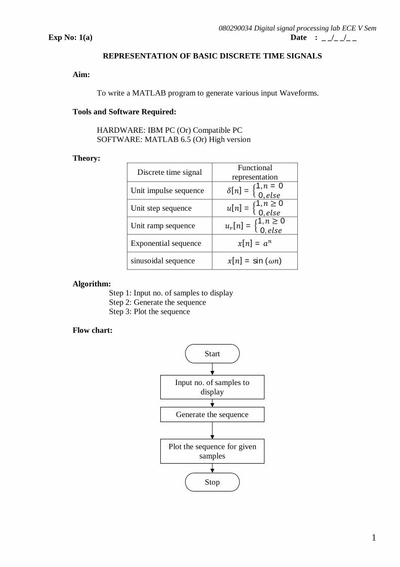
Flow chart:

Start

Input no. of samples to display

Generate the sequence

Plot the sequence for given samples

Stop


2

Program for Representation of basic discrete time signals: 1. %Function for Unit Impulse Sequence

function x=dt_ui(n) % Function for unit impulse sequence for i=1:length(n) if (n(i)-round(n(i)))~=0 x(i)=0; elseif n(i)==0 x(i)=1; else x(i)=0; end end

2. %Function for Unit step sequence function x=dt_us(n) % Function for unit step sequence for i=1:length(n) if (n(i)-round(n(i)))~=0 x(i)=0; elseif n(i)>=0 x(i)=1; else x(i)=0; end end

3. %Function for Unit Ramp sequence function x=dt_ur(n) % Function for unit ramp sequence for i=1:length(n) if (n(i)-round(n(i)))~=0 x(i)=0; elseif n(i)>=0 x(i)=n(i); else x(i)=0; end end

Procedure: 1. Write functions to generate unit impulse, unit step and unit ramp sequence and save each

function as separate file. 2. In Matlab goto FileNewFigure. 3. In figure window goto viewFigure palette. 4. In Figure palette window choose 2D axes 5. In the 2D axes obtained right click and choose add data 6. In the add data to axes dialog box choose plot type as stem and give samples to display in

x data source and generated sequence in the y data source 7. Insert x-label, y-label and title to the figure obtained.


3

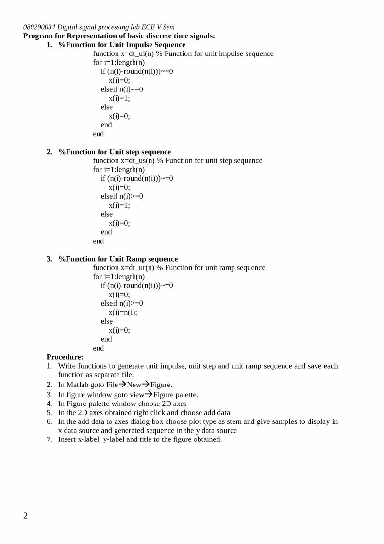
Output:

Result: Thus the MATLAB Program for representation of signals was written and verified.

Exercises: 1. Write a MATLAB program to represent unit step sequence (풖[풏]) and hence sketch the

following sequence 풙[풏] = 풖[풏] − ퟐ풖[풏 − ퟏ] + 풖[풏 − ퟒ]. 2. Write a MATLAB program to represent unit sample sequence (휹[풏]) and unit step sequence

(풖[풏]) and hence sketch the following sequence 풙[풏] = 휹[풏 + ퟏ]− 휹[풏] + 풖[풏 + ퟏ] − 풖[풏 − ퟐ].

3. Write a MATLAB program to represent unit step sequence (풖[풏]) and unit ramp sequence (풖풓[풏]) and hence sketch the following sequence 풙[풏] = 풖풓[풏 + ퟐ] − ퟐ풖[풏] − 풏풖[풏 − ퟒ].

4. Write a MATLAB program to represent unit step sequence (풖[풏]) and exponential sequence and hence sketch the following sequence 풙[풏] = 풆ퟎ.ퟖ풏풖[풏 + ퟏ] + 풖[풏].

5. Write a MATLAB program to represent sinusoidal sequence and exponential sequence and hence sketch the following sequence 풙[풏] = (ퟎ.ퟗ)풏[퐬퐢퐧(흅풏/ퟒ) + 퐜퐨퐬(흅풏/ퟒ)].

6. Write a MATLAB program to represent unit step sequence (풖[풏]) and exponential sequence and hence sketch the following sequence 풙[풏] = (−ퟎ.ퟓ)풏풖[풏].

-10 -5 0 5 100

0.5

1Unit Impulse Sequence

n

amp.

-10 -5 0 5 100

0.5

1Unit Step Sequence

n

amp.

-10 -5 0 5 100

5

10Unit Ramp Sequence

n

amp.

-10 -5 0 5 100

5

10Exponential (Growing)

n

amp.

-10 -5 0 5 100

5

10Exponential (Decaying)

n

amp.

-10 -5 0 5 10-1

0

1Sinusoidal

n

amp.


4

Exp No: 1(b) Date : _ _/_ _/_ _

GENERATION OF PERIODIC SIGNALS Aim:

To write a MATLAB program to generate various periodic signals.


HARDWARE: IBM PC (Or) Compatible PC SOFTWARE: MATLAB 6.5 (Or) High version

Theory:

Periodic sinusoidal sequence can be generated using the following iterative function sin(휔푛) = sin(휔(푛 − 1)) ∗ cos(휔) + cos(휔(푛 − 1)) ∗ sin(휔) cos(휔푛) = cos(휔(푛 − 1)) ∗ cos(휔) − sin(휔(푛 − 1)) ∗ sin (휔)

where, 휔 = ,푁 → period of the sequence (a rational number) Other periodic signals 푥(푡) can be generated using trigonometric Fourier series given

by

푥(푡) = 푎[0] + (푎[푛] cos(휔푛푡) + 푏[푛] sin(휔푛푡))

where, 휔 = ,푇 → period of the signal and

푎[0] = ∫ 푥(푡)푑푡

푎[푛] = ∫ 푥(푡)cos (푛휔푡) 푑푡,

푏[푛] = ∫ 푥(푡)sin (푛휔푡)푑푡 푎[0],푎[푛] 푎푛푑 푏[푛] are trigonometric Fourier series coefficients

Algorithm:

Step 1: Input period for the periodic signal Step 2: Generate the sinusoidal sequence for given period Step 3: Determine Fourier series coefficients for given periodic signal Step 4: Generate periodic signal using trigonometric Fourier series


5

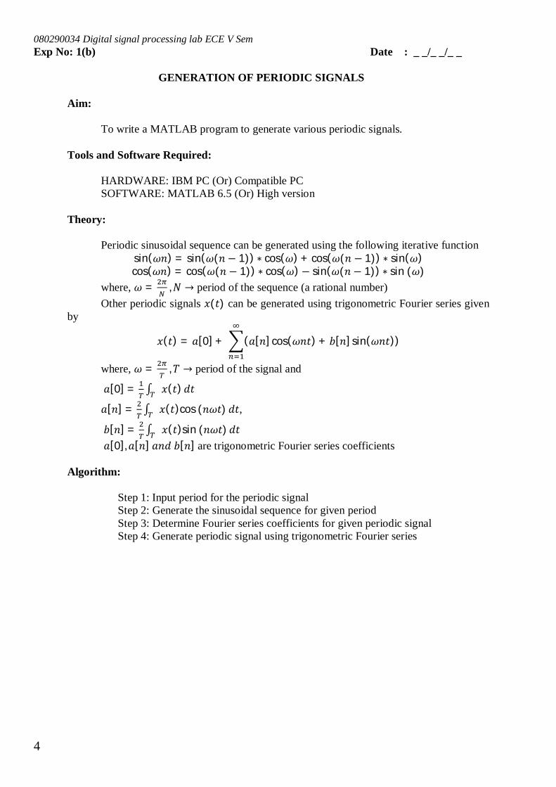
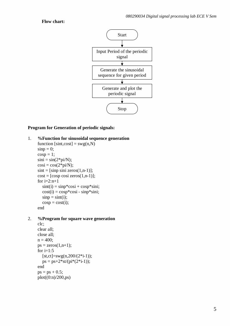
Flow chart:

Program for Generation of periodic signals: 1. %Function for sinusoidal sequence generation

function [sint,cost] = swg(n,N) sinp = 0; cosp = 1; sini = sin(2*pi/N); cosi = cos(2*pi/N); sint = [sinp sini zeros(1,n-1)]; cost = [cosp cosi zeros(1,n-1)]; for i=2:n+1 sint(i) = sinp*cosi + cosp*sini; cost(i) = cosp*cosi - sinp*sini; sinp = sint(i); cosp = cost(i); end

2. %Program for square wave generation clc; clear all; close all; n = 400; ps = zeros(1,n+1); for i=1:5 [st,ct]=swg(n,200/(2*i-1)); ps = ps+2*st/(pi*(2*i-1)); end ps = ps + 0.5; plot((0:n)/200,ps)

Start

Input Period of the periodic signal

Generate the sinusoidal sequence for given period

Generate and plot the periodic signal

Stop


6

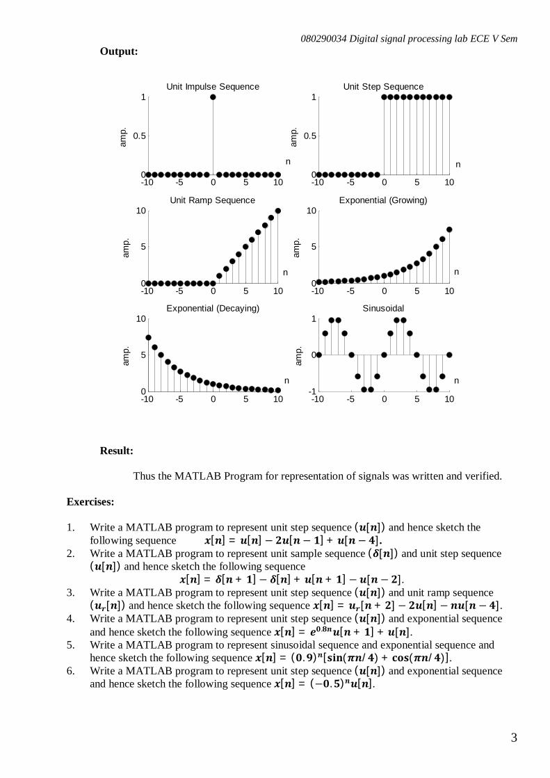
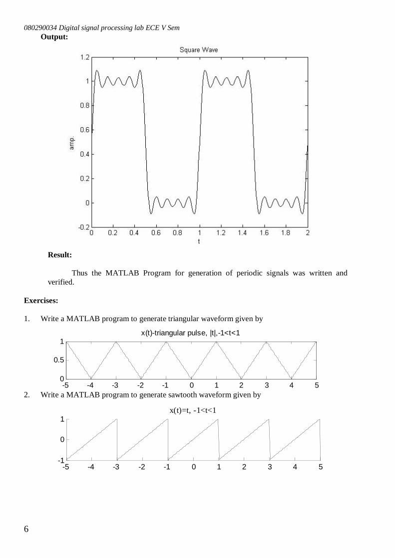
Output:

Result:

Thus the MATLAB Program for generation of periodic signals was written and verified.

Exercises: 1. Write a MATLAB program to generate triangular waveform given by

2. Write a MATLAB program to generate sawtooth waveform given by

-5 -4 -3 -2 -1 0 1 2 3 4 50

0.5

1x(t)-triangular pulse, |t|,-1<t<1

|c[n]|

-5 -4 -3 -2 -1 0 1 2 3 4 5-1

0

1x(t)=t, -1<t<1

|c[n]|


7

Exp No: 2 Date : _ _/_ _/_ _

VERIFICATION OF SAMPLING THEOREM

Aim: To write the program for verification of sampling theorem using MATLAB.


HARDWARE: IBM PC (OR) Compatible PC SOFTWARE: MATLAB 6.5 (OR) High version

Theory:

Discrete-time signal 푥[푛] is obtained by taking samples of analog signal 푥 (푡) every 푇 seconds, which is described by the relation

푥[푛] = 푥 (푛푇),−∞ < 푛 < ∞ The timing interval 푇 between successive samples is called the sampling period or

sampling interval and its reciprocal = 퐹 is called the sampling rate or the sampling frequency.

Let 퐹 be − < 퐹 < the frequencies 퐹 = 퐹 + 푘퐹 ,−∞ < 푘 < ∞, are indistinguishable from 퐹 after sampling and hence they are aliases of 퐹 .

Hence to avoid aliasing 퐹 is selected so that 퐹 > 2퐹 , where 퐹 is the largest frequency component in the analog signal 푥 (푡). Algorithm:

1. Choose fundamental frequency (F0) for a sinusoidal signal and sampling rate (Fs) according to Nyquist theorem.

2. Choose another sinusoidal signal of frequency F=F0+kFs, where k is an non-zero integer.

3. Display both sinusoidal signal for some time duration 0 to T. 4. Display the sampled sinusoidal signals for above time duration, sampled at the rate

Fs.


8

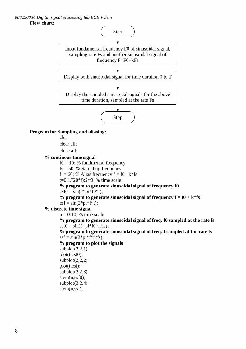
Flow chart:

Program for Sampling and aliasing: clc; clear all; close all;

% continous time signal f0 = 10; % fundmental frequency fs = 50; % Sampling frequency f = 60; % Alias frequency f = f0+ k*fs t=0:1/(20*f):2/f0; % time scale % program to generate sinusoidal signal of frequency f0 csf0 = sin(2*pi*f0*t); % program to generate sinusoidal signal of frequency f = f0 + k*fs csf = sin(2*pi*f*t);

% discrete time signal n = 0:10; % time scale % program to generate sinusoidal signal of freq. f0 sampled at the rate fs ssf0 = sin(2*pi*f0*n/fs); % program to generate sinusoidal signal of freq. f sampled at the rate fs ssf = sin(2*pi*f*n/fs); % program to plot the signals subplot(2,2,1) plot(t,csf0); subplot(2,2,2) plot(t,csf); subplot(2,2,3) stem(n,ssf0); subplot(2,2,4) stem(n,ssf);

Start

Input fundamental frequency F0 of sinusoidal signal, sampling rate Fs and another sinusoidal signal of

frequency F=F0+kFs

Display both sinusoidal signal for time duration 0 to T

Display the sampled sinusoidal signals for the above time duration, sampled at the rate Fs

Stop


9

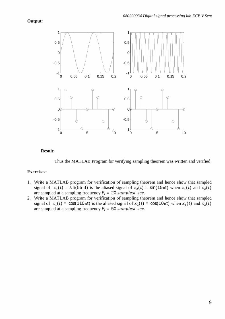
Output:

Result:

Thus the MATLAB Program for verifying sampling theorem was written and verified Exercises: 1. Write a MATLAB program for verification of sampling theorem and hence show that sampled

signal of 푥 (푡) = sin(55πt) is the aliased signal of 푥 (푡) = sin(15πt) when 푥 (푡) and 푥 (푡) are sampled at a sampling frequency 퐹 = 20 푠푎푚푝푙푒푠/ 푠푒푐.

2. Write a MATLAB program for verification of sampling theorem and hence show that sampled signal of 푥 (푡) = cos(110πt) is the aliased signal of 푥 (푡) = cos(10πt) when 푥 (푡) and 푥 (푡) are sampled at a sampling frequency 퐹 = 50 푠푎푚푝푙푒푠/ 푠푒푐.

0 0.05 0.1 0.15 0.2-1

-0.5

0

0.5

1

0 0.05 0.1 0.15 0.2-1

-0.5

0

0.5

1

0 5 10-1

-0.5

0

0.5

1

0 5 10-1

-0.5

0

0.5

1


10

Exp No: 3 Date : _ _/_ _/_ _

CALCULATION OF FFT AND IFFT OF A SEQUENCE Aim:

To write a MATLAB program for computing FFT of a Signal Tools and Software Required:


Theory:

N-point DFT of a discrete sequence 푥[푛] is given by

퐷퐹푇 푥[푛] = 푋[푘] = 푥[푛]푤 ,푤ℎ푒푟푒 푘 = 0,1, …푁 − 1 푎푛푑 푤 = 푒

N-point IDFT is given by

퐼퐷퐹푇 푋[푘] = 푥[푛] =1푁 푋[푘] 푤

∗,푤ℎ푒푟푒 푛 = 0,1, …푁 − 1

Algorithm:

1. Get the input sequence. 2. Compute the DFT and IDFT using FFT and IFFT fuction 3. Plot the input sequence, real part, imaginary part, magnitude spectrum and phase

spectrum of the DFT obtained and IFFT sequence obtained


11

Flow chart:

Program for calculation of FFT and IFFT: clc; clear all; close all; x = [1 2 1 2 1 2 1 2]; % enter the input sequence n=0:length(x)-1; X = fft(x); % DFT of the sequence y = ifft(X); % IDFT of the sequence % Program to plot the sequence subplot(3,2,1) stem(n,x); subplot(3,2,2) stem(n,real(X)); subplot(3,2,3) stem(n,imag(X)); subplot(3,2,4) stem(n,abs(X)); subplot(3,2,5) stem(n,angle(X)); subplot(3,2,6) stem(n,y);

Start

Input a sequence

Compute DFT and IDFT using FFT and IFFT

Plot the magnitude spectrum and Phase Spectrum for the DFT of the given input sequence

Stop


12

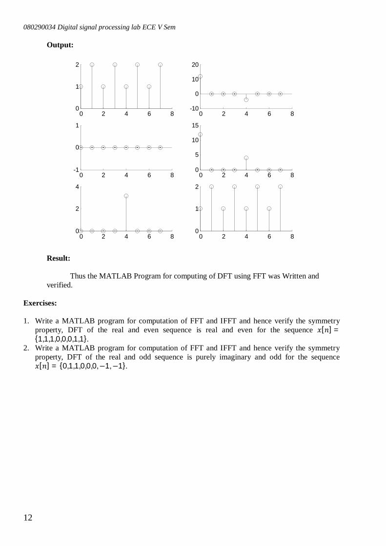
Output:

Result: Thus the MATLAB Program for computing of DFT using FFT was Written and verified.

Exercises: 1. Write a MATLAB program for computation of FFT and IFFT and hence verify the symmetry

property, DFT of the real and even sequence is real and even for the sequence 푥[푛] =1,1,1,0,0,0,1,1.

2. Write a MATLAB program for computation of FFT and IFFT and hence verify the symmetry property, DFT of the real and odd sequence is purely imaginary and odd for the sequence 푥[푛] = 0,1,1,0,0,0,−1,−1.

0 2 4 6 80

1

2

0 2 4 6 8-10

0

10

20

0 2 4 6 8-1

0

1

0 2 4 6 80

5

10

15

0 2 4 6 80

2

4

0 2 4 6 80

1

2


13

Exp No: 4 Date : _ _/_ _/_ _

TIME & FREQUENCY RESPONSE OF LTI SYSTEMS Aim:

To write a MATLAB program to compute time and frequency response of LTI system. Tools and Software Required:


Theory:

Time domain response ℎ[푛] of LTI system 퐻(푧) is given by

퐼푛푣푒푟푠푒 푧 푡푟푎푛푠푓표푟푚 퐻(푧) =푌(푧)푋(푧)

Frequency domain response 퐻(푒 ) of LTI system 퐻(푧) is given by

퐻 푒 =푌(푧)푋(푧)

Algorithm:

1. Get the Numerator and denominator coefficients of a LTI system 퐻(푧). 2. Compute impulse response h[n] of the LTI system 3. Compute frequency response 퐻(푒 ) of the LTI system 퐻(푧) 4. Plot the impulse response and magnitude and phase of frequency response


14

Flow chart:

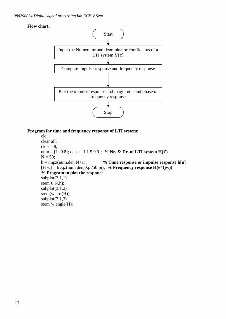
Program for time and frequency response of LTI system: clc; clear all; close all; num = [1 -0.8]; den = [1 1.5 0.9]; % Nr. & Dr. of LTI system H(Z) N = 50; h = impz(num,den,N+1); % Time response or impulse response h[n] [H w] = freqz(num,den,0:pi/50:pi); % Frequency response H(e^(jw)) % Program to plot the responce subplot(3,1,1) stem(0:N,h); subplot(3,1,2) stem(w,abs(H)); subplot(3,1,3) stem(w,angle(H));

Start

Input the Numerator and denominator coefficients of a LTI system 퐻(푧)

Compute impulse response and frequency response

Plot the impulse response and magnitude and phase of frequency response

Stop


15

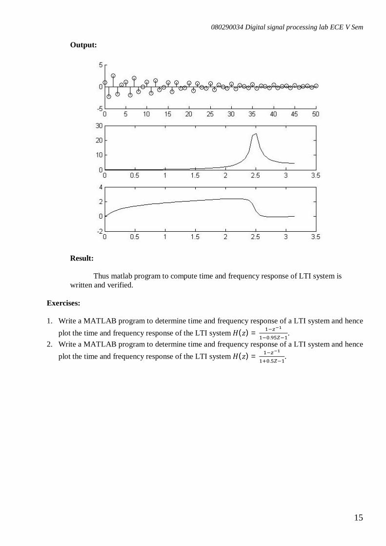
Output:

Result:

Thus matlab program to compute time and frequency response of LTI system is written and verified.

Exercises: 1. Write a MATLAB program to determine time and frequency response of a LTI system and hence

plot the time and frequency response of the LTI system 퐻(푧) =.

. 2. Write a MATLAB program to determine time and frequency response of a LTI system and hence

plot the time and frequency response of the LTI system 퐻(푧) =.

.


16

Exp No: 5 Date : _ _/_ _/_ _

LINEAR AND CIRCULAR CONVOLUTION THROUGH FFT Aim:

To write a program for linear convolution and circular convolution using MATLAB. Tools and Software Required:


Theory:

Linear convolution 푦[푛] for the sequence 푥[푛] and ℎ[푛] is given by 푦[푛] = ∑ 푥[푘]ℎ[푛 − 푘] (1)

N-point Circular convolution 푦[푛] for the sequence 푥[푛] and ℎ[푛] is given by 푦[푛] = ∑ 푥[푘]ℎ[(푛 − 푘) ] ,푤ℎ푒푟푒 푛 = 0,1, …푁 − 1 (2)

Using circular convolution property of DFT circular convolution 푦[푛] is obtained by 푦[푛] = 퐼퐷퐹푇[퐷퐹푇(푥[푛] )퐷퐹푇(ℎ[푛] )] (3)

Linear convolution 푦[푛] for the sequence 푥[푛] of length m and ℎ[푛] of length l is obtained by computing N-point circular convolution between x[n] and h[n], where N = m+l-1. Algorithm:

1. Enter the value for the sequence 푥[푛] and ℎ[푛]. 2. Compute the linear convolution using the equation (1) 3. Compute the circular convolution using the equation (2) 4. Verify the result through circular convolution property of DFT 5. Display the input sequences, output linear and circular convolution sequences.

Flow chart:

Start

Input a sequence x and h

Compute Linear convolution and circular convolution using equation (1) & (2)

Compute Linear convolution and circular convolution using circular convolution property of DFT

Stop


17

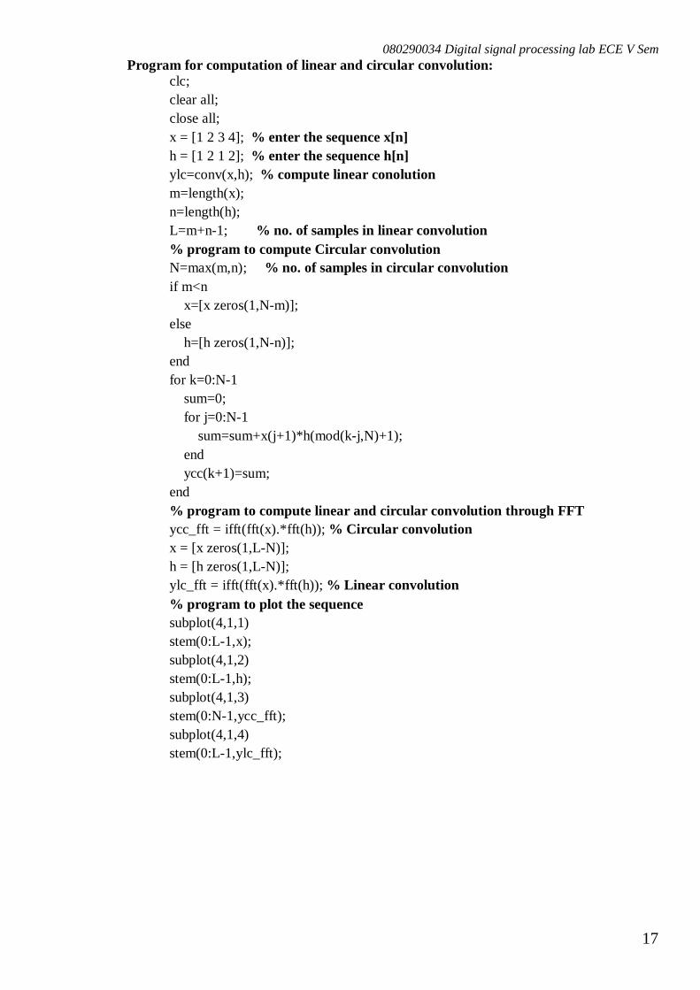
Program for computation of linear and circular convolution: clc; clear all; close all; x = [1 2 3 4]; % enter the sequence x[n] h = [1 2 1 2]; % enter the sequence h[n] ylc=conv(x,h); % compute linear conolution m=length(x); n=length(h); L=m+n-1; % no. of samples in linear convolution % program to compute Circular convolution N=max(m,n); % no. of samples in circular convolution if m<n x=[x zeros(1,N-m)]; else h=[h zeros(1,N-n)]; end for k=0:N-1 sum=0; for j=0:N-1 sum=sum+x(j+1)*h(mod(k-j,N)+1); end ycc(k+1)=sum; end % program to compute linear and circular convolution through FFT ycc_fft = ifft(fft(x).*fft(h)); % Circular convolution x = [x zeros(1,L-N)]; h = [h zeros(1,L-N)]; ylc_fft = ifft(fft(x).*fft(h)); % Linear convolution % program to plot the sequence subplot(4,1,1) stem(0:L-1,x); subplot(4,1,2) stem(0:L-1,h); subplot(4,1,3) stem(0:N-1,ycc_fft); subplot(4,1,4) stem(0:L-1,ylc_fft);


18

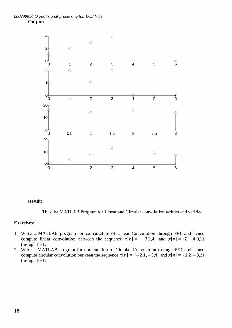
Output:

Result: Thus the MATLAB Program for Linear and Circular convolution written and verified.

Exercises: 1. Write a MATLAB program for computation of Linear Convolution through FFT and hence

compute linear convolution between the sequence 푥[푛] = −3,2,4 and 푥[푛] = 2,−4,0,1 through FFT.

2. Write a MATLAB program for computation of Circular Convolution through FFT and hence compute circular convolution between the sequence 푥[푛] = −2,1,−3,4 and 푥[푛] = 1,2,−3,2 through FFT.

0 1 2 3 4 5 60

2

4

0 1 2 3 4 5 60

1

2

0 0.5 1 1.5 2 2.5 30

10

20

0 1 2 3 4 5 60

10

20


19

Exp No: 6 Date : _ _/_ _/_ _

Design of FIR filter using windows Aim:

To write a MATLAB program to design a FIR filter by using Windowing techniques. Tools and Software Required:


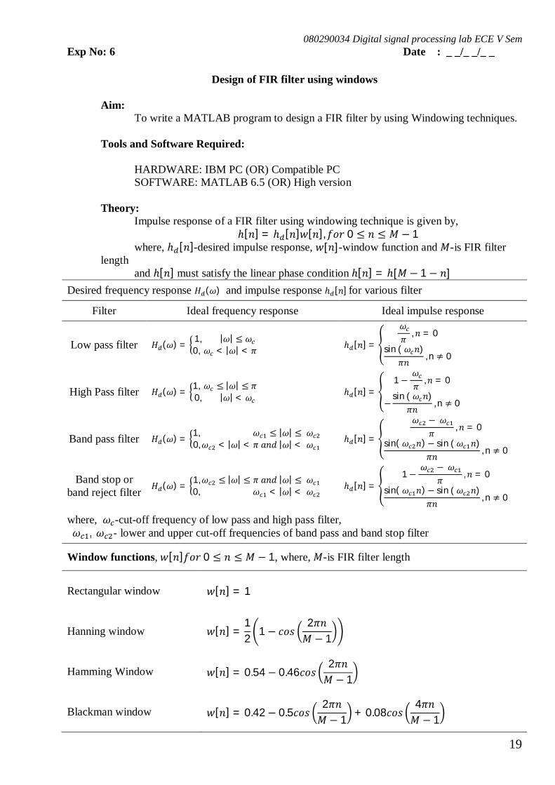
Theory:

Impulse response of a FIR filter using windowing technique is given by, ℎ[푛] = ℎ [푛]푤[푛],푓표푟 0 ≤ 푛 ≤ 푀 − 1

where, ℎ [푛]-desired impulse response, 푤[푛]-window function and 푀-is FIR filter length

and ℎ[푛] must satisfy the linear phase condition ℎ[푛] = ℎ[푀− 1 − 푛] Desired frequency response 퐻 (휔) and impulse response ℎ [푛] for various filter

Filter Ideal frequency response Ideal impulse response

Low pass filter 퐻 (휔) = 1, |휔| ≤ 휔0, 휔 < |휔| < 휋 ℎ [푛] =

휔휋 , 푛 = 0

sin ( 휔 푛)휋푛 , n ≠ 0

High Pass filter 퐻 (휔) = 1, 휔 ≤ |휔| ≤ 휋0, |휔| < 휔 ℎ [푛] =

1− 휔휋 ,푛 = 0

−sin ( 휔 푛)

휋푛 , n ≠ 0

Band pass filter 퐻 (휔) = 1, 휔 ≤ |휔| ≤ 휔0,휔 < |휔| < 휋 푎푛푑 |휔| < 휔 ℎ [푛] =

휔 − 휔휋 , 푛 = 0

sin( 휔 푛)− sin ( 휔 푛)휋푛 , n ≠ 0

Band stop or band reject filter 퐻 (휔) = 1,휔 ≤ |휔| ≤ 휋 푎푛푑 |휔| ≤ 휔

0, 휔 < |휔| < 휔 ℎ [푛] =1−

휔 − 휔휋 ,푛 = 0

sin( 휔 푛)− sin ( 휔 푛)휋푛 , n ≠ 0

where, 휔 -cut-off frequency of low pass and high pass filter, 휔 , 휔 - lower and upper cut-off frequencies of band pass and band stop filter

Window functions, 푤[푛]푓표푟 0 ≤ 푛 ≤ 푀 − 1, where, 푀-is FIR filter length

Rectangular window 푤[푛] = 1

Hanning window 푤[푛] =12 1 − 푐표푠

2휋푛푀 − 1

Hamming Window 푤[푛] = 0.54 − 0.46푐표푠2휋푛푀 − 1

Blackman window 푤[푛] = 0.42 − 0.5푐표푠2휋푛푀 − 1 + 0.08푐표푠

4휋푛푀 − 1


20

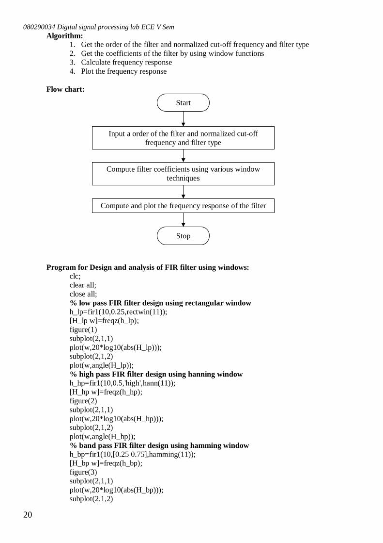
Algorithm: 1. Get the order of the filter and normalized cut-off frequency and filter type 2. Get the coefficients of the filter by using window functions 3. Calculate frequency response 4. Plot the frequency response

Flow chart:

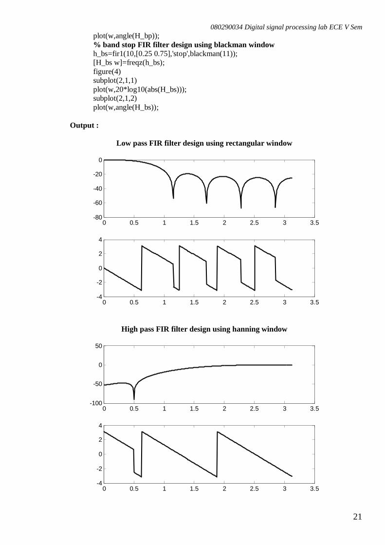
Program for Design and analysis of FIR filter using windows: clc; clear all; close all; % low pass FIR filter design using rectangular window h_lp=fir1(10,0.25,rectwin(11)); [H_lp w]=freqz(h_lp); figure(1) subplot(2,1,1) plot(w,20*log10(abs(H_lp))); subplot(2,1,2) plot(w,angle(H_lp)); % high pass FIR filter design using hanning window h_hp=fir1(10,0.5,'high',hann(11)); [H_hp w]=freqz(h_hp); figure(2) subplot(2,1,1) plot(w,20*log10(abs(H_hp))); subplot(2,1,2) plot(w,angle(H_hp)); % band pass FIR filter design using hamming window h_bp=fir1(10,[0.25 0.75],hamming(11)); [H_bp w]=freqz(h_bp); figure(3) subplot(2,1,1) plot(w,20*log10(abs(H_bp))); subplot(2,1,2)

Start

Input a order of the filter and normalized cut-off frequency and filter type

Compute filter coefficients using various window techniques

Compute and plot the frequency response of the filter

Stop


21

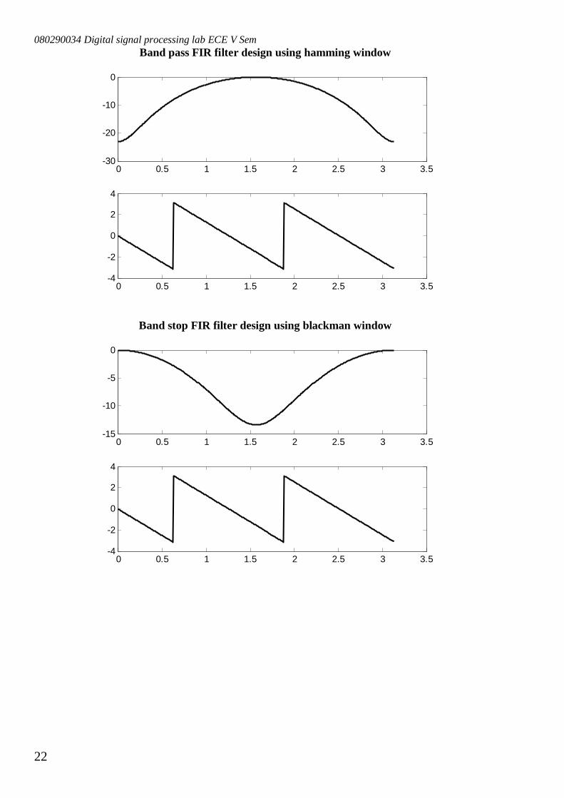
plot(w,angle(H_bp)); % band stop FIR filter design using blackman window h_bs=fir1(10,[0.25 0.75],'stop',blackman(11)); [H_bs w]=freqz(h_bs); figure(4) subplot(2,1,1) plot(w,20*log10(abs(H_bs))); subplot(2,1,2) plot(w,angle(H_bs));

Output :

Low pass FIR filter design using rectangular window

High pass FIR filter design using hanning window

0 0.5 1 1.5 2 2.5 3 3.5-80

-60

-40

-20

0

0 0.5 1 1.5 2 2.5 3 3.5-4

-2

0

2

4

0 0.5 1 1.5 2 2.5 3 3.5-100

-50

0

50

0 0.5 1 1.5 2 2.5 3 3.5-4

-2

0

2

4


22

Band pass FIR filter design using hamming window

Band stop FIR filter design using blackman window

0 0.5 1 1.5 2 2.5 3 3.5-30

-20

-10

0

0 0.5 1 1.5 2 2.5 3 3.5-4

-2

0

2

4

0 0.5 1 1.5 2 2.5 3 3.5-15

-10

-5

0

0 0.5 1 1.5 2 2.5 3 3.5-4

-2

0

2

4


23

Result:

Thus the MATLAB Program for FIR filter using windowing techniques is designed and verified.

Exercises: 1. Write a MATLAB program to design digital high pass Linear phase FIR filter with cut-off

frequency 휔 = . Using rectangular window of length 11. 2. Write a MATLAB program to design digital low pass Linear phase FIR filter with cut-off

frequency 휔 = 0.5휋. Using Hamming window of length 9. 3. Write a MATLAB program to design digital band pass Linear phase FIR filter with cut-off

frequencies 휔 = 0.25휋 and 휔 = 0.75휋. Using Hanning window of length 11. 4. Write a MATLAB program to design digital band stop Linear phase FIR filter with cut-off

frequencies 휔 = and 휔 = . Using Blackman window of length 9.


24

Exp No: 7 Date : _ _/_ _/_ _ Design of IIR filters from Chebychev analog filters

Aim:

To write a program to design a chebyshev low pass filter 1.Impulse invariant method 2.Bilinear Transform using MATLAB.



Theory: Type I Chebyshev filters are all-pole filters that exhibit equiripple behavior in the passband and a monotonic characteristics in the stopband. The magnitude squared of the frequency response is given as,

|퐻(Ω)| =1

1 + 휀 푇 Ω Ω⁄

Where, 푇 (푥) is the 푁th-order Chebyshev polynomial Order of the filter is given by,

푁 =푐표푠ℎ (훿 휀⁄ )푐표푠ℎ (Ω Ω )⁄

Where, 훿 = − 1 and 훿 -is the stop band ripple

휀 =( )

− 1 and 훿 -is the pass band ripple

Ω -is the stop band edge frequency Ω -is the pass band edge frequency Poles of the type I Chebyshev filter lie on the ellipse at the coordinates (푥 ,푦 ) given as,

푥 = 푟 cos휑 푘 = 0,1, … ,푁 − 1 푦 = 푟 sin휑 , 푘 = 0,1, … ,푁 − 1

Where, 휑 = + ( ) is the angular positions of the poles

푟 = Ω is the semi major axis of the ellipse

푟 = Ω is the semi minor axis of the ellipse and 훽 = √⁄

Hence, analog system transfer function of type I chebyshev filter is given by,

퐻 (푠) =1

∏ (푠 − 푠 )

Where, 푠 = 푥 +푗푦 are poles of the filter. Impulse invariance – used to determine system transfer function of digital IIR filter

퐻(푧) from analog system transfer function using the relation 퐻(푧) = 퐻 (푠)|

∑ ∑

and digital frequency, 휔 = Ω푇, where, Ω - is analog frequency and 푇 - is sampling period.

Bilinear transformation – used to determine system transfer function of digital IIR filter 퐻(푧) from analog system transfer function using the relation

퐻(푧) = 퐻 (푠)|


25

and digital frequency, 휔 = 2푡푎푛 , where, Ω - is analog frequency and 푇 - is sampling period.

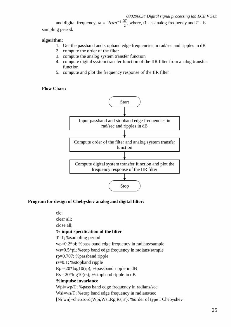
algorithm:

1. Get the passband and stopband edge frequencies in rad/sec and ripples in dB 2. compute the order of the filter 3. compute the analog system transfer function 4. compute digital system transfer function of the IIR filter from analog transfer

function 5. compute and plot the frequency response of the IIR filter

Flow Chart:

Program for design of Chebyshev analog and digital filter:

clc; clear all; close all; % input specification of the filter T=1; %sampling period wp=0.2*pi; %pass band edge frequency in radians/sample ws=0.5*pi; %stop band edge frequency in radians/sample rp=0.707; %passband ripple rs=0.1; %stopband ripple Rp=-20*log10(rp); %passband ripple in dB Rs=-20*log10(rs); %stopband ripple in dB %impulse invariance Wpi=wp/T; %pass band edge frequency in radians/sec Wsi=ws/T; %stop band edge frequency in radians/sec [Ni wn]=cheb1ord(Wpi,Wsi,Rp,Rs,'s'); %order of type I Chebyshev

Start

Input passband and stopband edge frequencies in rad/sec and ripples in dB

Compute order of the filter and analog system transfer function

Compute digital system transfer function and plot the frequency response of the IIR filter

Stop


26

[bi ai]=cheby1(Ni,rp,wn,'s'); %analog transfer function of type I Chebyshev [Bi Ai]=impinvar(bi,ai,1/T); %digital transfer function using impulse invariance [Hi w]=freqz(Bi,Ai); %frequency response figure(1); subplot(2,1,1) plot(w,20*log10(abs(Hi))); subplot(2,1,2) plot(w,angle(Hi)); %Bilinear transformantion Wpb=(2/T)*tan(wp/2); %pass band edge frequency in radians/sec Wsb=(2/T)*tan(ws/2); %stop band edge frequency in radians/sec [Nb wn]=cheb1ord(Wpb,Wsb,Rp,Rs,'s'); %order of type I Chebyshev [bb ab]=cheby1(Nb,rp,wn,'s'); %analog transfer function of type I Chebyshev [Bb Ab]=bilinear(bb,ab,1/T); %digital transfer function using impulse invariance [Hb w]=freqz(Bb,Ab); %frequency response figure(2); subplot(2,1,1) plot(w,20*log10(abs(Hb))); subplot(2,1,2) plot(w,angle(Hb));

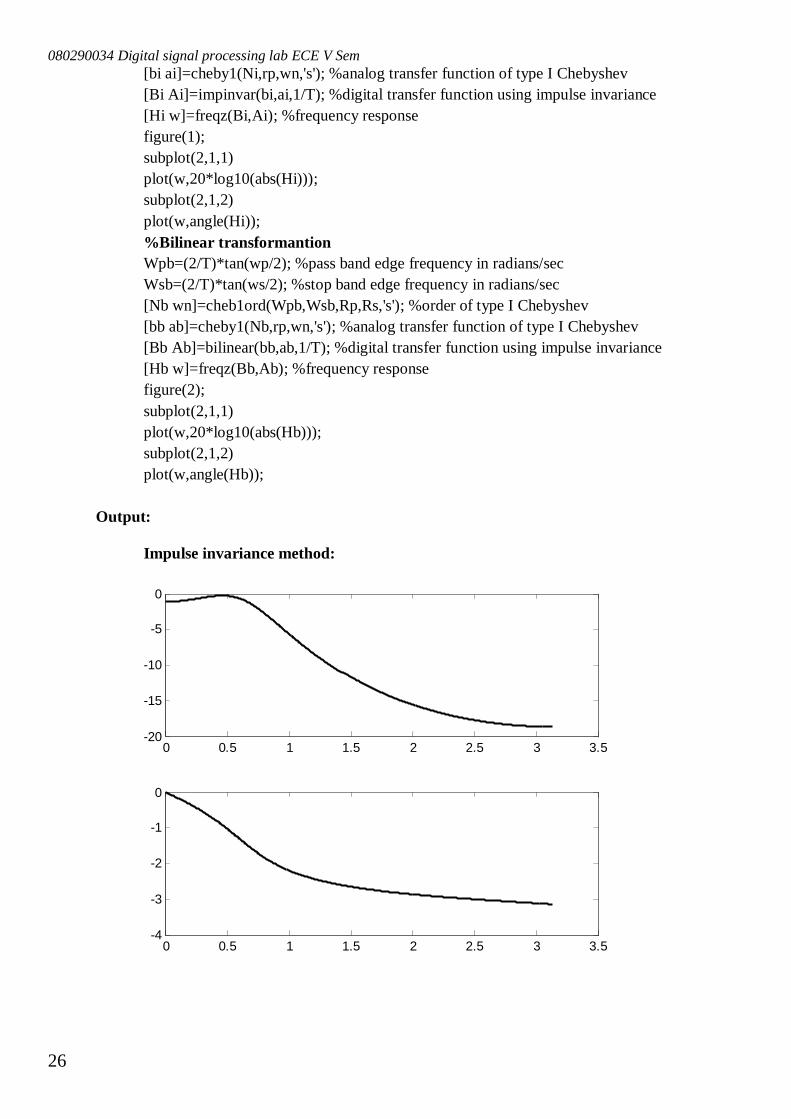
Output:

Impulse invariance method:

0 0.5 1 1.5 2 2.5 3 3.5-20

-15

-10

-5

0

0 0.5 1 1.5 2 2.5 3 3.5-4

-3

-2

-1

0


27

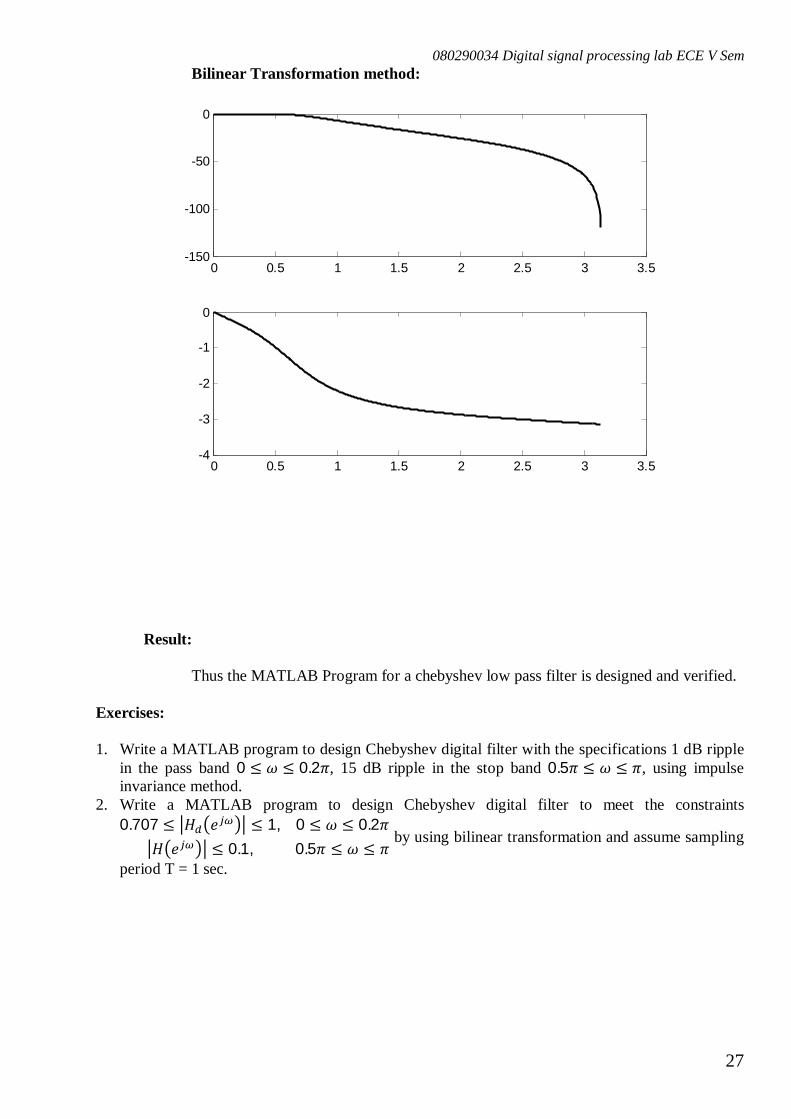
Bilinear Transformation method:

Result:

Thus the MATLAB Program for a chebyshev low pass filter is designed and verified.

Exercises: 1. Write a MATLAB program to design Chebyshev digital filter with the specifications 1 dB ripple

in the pass band 0 ≤ 휔 ≤ 0.2휋, 15 dB ripple in the stop band 0.5휋 ≤ 휔 ≤ 휋, using impulse invariance method.

2. Write a MATLAB program to design Chebyshev digital filter to meet the constraints 0.707 ≤ 퐻 푒 ≤ 1, 0 ≤ 휔 ≤ 0.2휋

퐻 푒 ≤ 0.1, 0.5휋 ≤ 휔 ≤ 휋 by using bilinear transformation and assume sampling

period T = 1 sec.

0 0.5 1 1.5 2 2.5 3 3.5-150

-100

-50

0

0 0.5 1 1.5 2 2.5 3 3.5-4

-3

-2

-1

0


28

Exp No: 8 Date : _ _/_ _/_ _

Design of IIR filters from Butterworth analog filters Aim:

To write a program for Butterworth low pass filter by i) Impulse invariant method ii) Bilinear Transform using MATLAB.



Theory: Butterworth filters are all-pole filters and monotonic in both the passband and stopband. The magnitude squared of the frequency response is given as,

|퐻(Ω)| =1

1 + (Ω Ω⁄ )

Where, Ω is the 3-dB cut-off frequency in rad/sec Order of the filter is given by,

푁 =푙표푔(훿 휀⁄ )푙표푔(Ω Ω )⁄

Where, 훿 = − 1 and 훿 -is the stop band ripple

휀 =( )

− 1 and 훿 -is the pass band ripple

Ω -is the stop band edge frequency Ω -is the pass band edge frequency Poles of the butterworth filter lie on the circle of radius Ω at the coordinates (푥 , 푦 ) given as,

푥 = Ω cos휑 푘 = 0,1, … ,푁 − 1 푦 = Ω sin휑 , 푘 = 0,1, … ,푁 − 1

Where, 휑 = + ( ) is the angular positions of the poles Hence, analog system transfer function of butterworth filter is given by,

퐻 (푠) =1

∏ (푠 − 푠 )

Where, 푠 = 푥 +푗푦 are poles of the filter. Impulse invariance – used to determine system transfer function of digital IIR filter

퐻(푧) from analog system transfer function using the relation 퐻(푧) = 퐻 (푠)|

∑ ∑

and digital frequency, 휔 = Ω푇, where, Ω - is analog frequency and 푇 - is sampling period.

Bilinear transformation – used to determine system transfer function of digital IIR filter 퐻(푧) from analog system transfer function using the relation

퐻(푧) = 퐻 (푠)|

and digital frequency, 휔 = 2푡푎푛 , where, Ω - is analog frequency and 푇 - is sampling period.


29

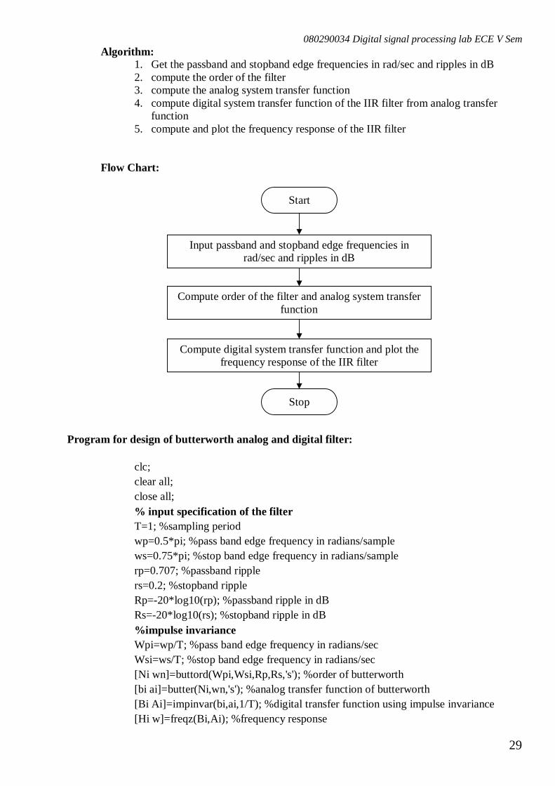
Algorithm: 1. Get the passband and stopband edge frequencies in rad/sec and ripples in dB 2. compute the order of the filter 3. compute the analog system transfer function 4. compute digital system transfer function of the IIR filter from analog transfer

function 5. compute and plot the frequency response of the IIR filter

Flow Chart:

Program for design of butterworth analog and digital filter:

clc; clear all; close all; % input specification of the filter T=1; %sampling period wp=0.5*pi; %pass band edge frequency in radians/sample ws=0.75*pi; %stop band edge frequency in radians/sample rp=0.707; %passband ripple rs=0.2; %stopband ripple Rp=-20*log10(rp); %passband ripple in dB Rs=-20*log10(rs); %stopband ripple in dB %impulse invariance Wpi=wp/T; %pass band edge frequency in radians/sec Wsi=ws/T; %stop band edge frequency in radians/sec [Ni wn]=buttord(Wpi,Wsi,Rp,Rs,'s'); %order of butterworth [bi ai]=butter(Ni,wn,'s'); %analog transfer function of butterworth [Bi Ai]=impinvar(bi,ai,1/T); %digital transfer function using impulse invariance [Hi w]=freqz(Bi,Ai); %frequency response

Start

Input passband and stopband edge frequencies in rad/sec and ripples in dB

Compute order of the filter and analog system transfer function

Compute digital system transfer function and plot the frequency response of the IIR filter

Stop


30

figure(1); subplot(2,1,1) plot(w,20*log10(abs(Hi))); subplot(2,1,2) plot(w,angle(Hi)); %Bilinear transformantion Wpb=(2/T)*tan(wp/2); %pass band edge frequency in radians/sec Wsb=(2/T)*tan(ws/2); %stop band edge frequency in radians/sec [Nb wn]=buttord(Wpb,Wsb,Rp,Rs,'s'); %order of butterworth [bb ab]=butter(Nb,wn,'s'); %analog transfer function of butterworth [Bb Ab]=bilinear(bb,ab,1/T); %digital transfer function using impulse invariance [Hb w]=freqz(Bb,Ab); %frequency response figure(2); subplot(2,1,1) plot(w,20*log10(abs(Hb))); subplot(2,1,2) plot(w,angle(Hb));

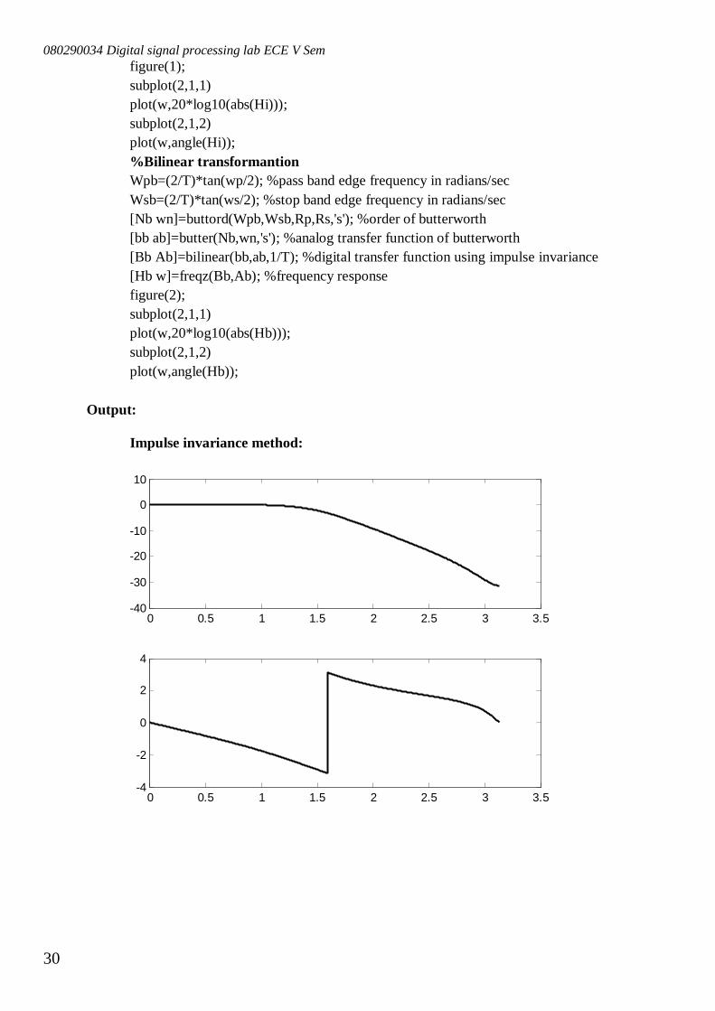
Output:

Impulse invariance method:

0 0.5 1 1.5 2 2.5 3 3.5-40

-30

-20

-10

0

10

0 0.5 1 1.5 2 2.5 3 3.5-4

-2

0

2

4


31

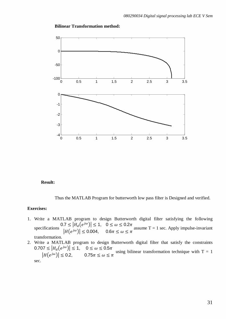
Bilinear Transformation method:

Result:

Thus the MATLAB Program for butterworth low pass filter is Designed and verified. Exercises: 1. Write a MATLAB program to design Butterworth digital filter satisfying the following

specifications 0.7 ≤ 퐻 푒 ≤ 1, 0 ≤ 휔 ≤ 0.2휋퐻 푒 ≤ 0.004, 0.6휋 ≤ 휔 ≤ 휋

assume T = 1 sec. Apply impulse-invariant

transformation. 2. Write a MATLAB program to design Butterworth digital filter that satisfy the constraints

0.707 ≤ 퐻 푒 ≤ 1, 0 ≤ 휔 ≤ 0.5휋퐻 푒 ≤ 0.2, 0.75휋 ≤ 휔 ≤ 휋

using bilinear transformation technique with T = 1

sec.

0 0.5 1 1.5 2 2.5 3 3.5-100

-50

0

50

0 0.5 1 1.5 2 2.5 3 3.5-4

-3

-2

-1

0


32

INTRODUCTION TO CODE COMPOSER STUDIO

Code Composer is the DSP industry’s first fully integrated development environment (IDE) with DSP-specific functionality. With a familiar environment liked MS-based C++TM, Code Composer lets you edit, build, debug, profile and manage projects from a single unified environment. Other unique features include graphical signal analysis, injection/extraction of data signals via file I/O, multi-processor debugging, automated testing and customization via a C-interpretive scripting language and much more. PROCEDURE TO WORK ON CODE COMPOSER STUDIO To create the New Project

Project → New (File Name. pjt , Eg: Vectors.pjt) To Create a Source file

File → New → Type the code (Save & give file name, Eg: sum.c). To Add Source files to Project

Project → Add files to Project → sum.c To Add library file & command file:

Project → Add files to Project → rts500.lib Library files: rts500.lib (Path: C:\CCStudio_v3.1\C5400\cgtools\lib\rts500.lib) Note: Select Object & Library in(*.o,*.l) in Type of files

Project → Add files to Project → c5416dsk.cmd CMD file . Which is common for all non real time programs. (Path: C:\CCStudio_v3.1\tutorial\dsk5416\shared\c5416dsk.cmd) Note: Select Linker Command file(*.cmd) in Type of files

Compile: To Compile: Project → Compile To build: Project → build,

Which will create the final .out executable file.(Eg. Vectors.out). Procedure to Load and Run program:

Load the program to DSK: File → Load program → Vectors.out To Execute project: Debug → Run.

To View output graphically Select view → graph → time and frequency

In the Graph Property Dialog box enter the Graph Title start address Acquistion buffer size Display data size DSP datatype Data plot style

This values for the sequence obtained using watch window in the menu View→Watch Window


33

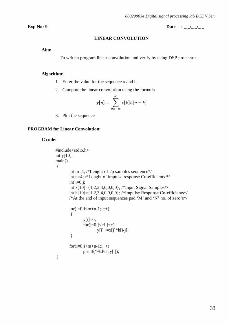
Exp No: 9 Date : _ _/_ _/_ _

LINEAR CONVOLUTION

Aim:

To write a program linear convolution and verify by using DSP processor.

Algorithm:

1. Enter the value for the sequence x and h.

2. Compute the linear convolution using the formula

푦[푛] = 푥[푘]ℎ[푛 − 푘]

3. Plot the sequence

PROGRAM for Linear Convolution:

C code:

#include<stdio.h> int y[10]; main()

int m=4; /*Lenght of i/p samples sequence*/ int n=4; /*Lenght of impulse response Co-efficients */ int i=0,j; int x[10]=1,2,3,4,0,0,0,0; /*Input Signal Samples*/ int h[10]=1,2,3,4,0,0,0,0; /*Impulse Response Co-efficients*/ /*At the end of input sequences pad ‘M’ and ‘N’ no. of zero’s*/ for(i=0;i<m+n-1;i++)

y[i]=0; for(j=0;j<=i;j++)

y[i]+=x[j]*h[i-j]; for(i=0;i<m+n-1;i++)

printf("%d\n",y[i]);


34

Output:

Result: Thus program for linear convolution using DSP processor was written and verified.


35

Exp No: 10 Date : _ _/_ _/_ _

CIRCULAR CONVOLUTION

Aim:

To write a program for circular convolution and verify by using DSP processor.

Algorithm:

4. Enter the value for the sequence x and h.

5. Compute the circular convolution using the formula

푦[푛] = 푥[푘]ℎ[(푛 − 푘) ] ,푤ℎ푒푟푒 푛 = 0,1, …푁 − 1

6. Plot the sequence

PROGRAM FOR CIRCULAR CONVOLUTION

C code:

#include<stdio.h> int m,n,x[30],h[30],y[30],i,j,temp[30],k,x2[30],a[30]; void main()

printf(" enter the length of the first sequence\n"); scanf("%d",&m); printf(" enter the length of the second sequence\n"); scanf("%d",&n); printf(" enter the first sequence\n"); for(i=0;i<m;i++)

scanf("%d",&x[i]); printf(" enter the second sequence\n"); for(j=0;j<n;j++)

scanf("%d",&h[j]); if(m-n!=0) /*If length of both sequences are not equal*/

if(m>n) /* Pad the smaller sequence with zero*/

for(i=n;i<m;i++) h[i]=0;

n=m; else

for(i=m;i<n;i++) x[i]=0;

m=n;

y[0]=0;


36

a[0]=h[0]; for(j=1;j<n;j++) /*folding h(n) to h(-n)*/

a[j]=h[n-j]; /*Circular convolution*/ for(i=0;i<n;i++)

y[0]+=x[i]*a[i]; for(k=1;k<n;k++)

y[k]=0; /*circular shift*/ for(j=1;j<n;j++)

x2[j]=a[j-1]; x2[0]=a[n-1]; for(i=0;i<n;i++)

a[i]=x2[i]; y[k]+=x[i]*x2[i];

/*displaying the result*/ printf(" the circular convolution is\n"); for(i=0;i<n;i++)

printf("%d \t",y[i]);

Input:

x[4]=3, 2, 1, 0 h[4]=1, 1, 0, 0

Output:

y[4]=3, 5, 3, 1

Result: Thus program for circular convolution using DSP processor was written and verified.


37

Exp No: 11 Date : _ _/_ _/_ _

CALCULATION OF FFT

Aim:

To write a program for calculation of FFT and verify by using DSP processor. Algorithm:

1. Get the input sinusoidal sequence. 2. Compute the DFT using the DIF FFT algorithm 3. Plot the magnitude spectrum of the DFT obtained

PROGRAM calculation of FFT: C Code:

#include <stdio.h> #include <math.h> #define n 8 float x[n][2]; float y[n][2]; float mag[n]; main() int i,j,k,m,p,q,r; float a1,a2,b1,b2,c1,c2,d1,d2,w1,w2; float x1[n][2],y1[n][2]; for (i=0;i<n;i++) //scanf("%f",&x[i][0]); x[i][0]=sin(2*3.14*3*i/8)+sin(2*3.14*1*i/8); x[i][1]=0; x1[i][0]=0; x1[i][1]=0; // DIF algorithm for FFT m=log(n)/log(2); for (i=0;i<m;i++) q=n/pow(2,i); for (j=0;j<n;j=j+q) r=j; for(k=0;k<q/2;k++) a1=x[r][0]; a2=x[r][1]; b1=x[r+q/2][0]; b2=x[r+q/2][1]; w1=cos(2*3.14*k/q); w2=sin(2*3.14*k/q); c1=a1+b1;


38

c2=a2+b2; d1=a1-b1; d2=a2-b2; x1[r][0]=c1; x1[r][1]=c2; x1[r+q/2][0]=d1*w1+d2*w2; x1[r+q/2][1]=d2*w1-d1*w2; r=r+1; for(p=0;p<n;p++) x[p][0]=x1[p][0]; x[p][1]=x1[p][1]; y[p][0]=x1[p][0]; y[p][1]=x1[p][1]; x1[p][0]=0; x1[p][1]=0; // Output into normal order for (i=0;i<m;i++) q=n/pow(2,i); for (j=0;j<n;j=j+q) r=j; for(k=0;k<q/2;k++) y1[r][0]=y[2*k+j][0]; y1[r][1]=y[2*k+j][1]; y1[r+q/2][0]=y[2*k+1+j][0]; y1[r+q/2][1]=y[2*k+1+j][1]; r=r+1; for(p=0;p<n;p++) y[p][0]=y1[p][0]; y[p][1]=y1[p][1]; y1[p][0]=0; y1[p][1]=0; for(p=0;p<n;p++) mag[p]=sqrt(y[p][0]*y[p][0]+y[p][1]*y[p][1]);


39

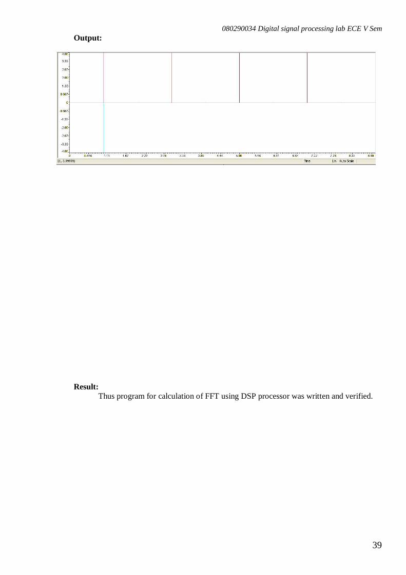
Output:

Result: Thus program for calculation of FFT using DSP processor was written and verified.


40

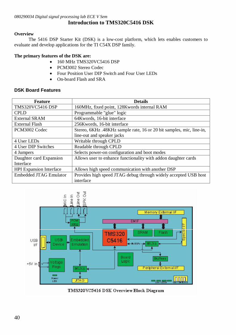
Introduction to TMS320C5416 DSK Overview

The 5416 DSP Starter Kit (DSK) is a low-cost platform, which lets enables customers to evaluate and develop applications for the TI C54X DSP family. The primary features of the DSK are:

160 MHz TMS320VC5416 DSP PCM3002 Stereo Codec Four Position User DIP Switch and Four User LEDs On-board Flash and SRA

DSK Board Features

Feature Details TMS320VC5416 DSP 160MHz, fixed point, 128Kwords internal RAM CPLD Programmable "glue" logic External SRAM 64Kwords, 16-bit interface External Flash 256Kwords, 16-bit interface PCM3002 Codec Stereo, 6KHz .48KHz sample rate, 16 or 20 bit samples, mic, line-in,

line-out and speaker jacks 4 User LEDs Writable through CPLD 4 User DIP Switches Readable through CPLD 4 Jumpers Selects power-on configuration and boot modes Daughter card Expansion Interface

Allows user to enhance functionality with addon daughter cards

HPI Expansion Interface Allows high speed communication with another DSP Embedded JTAG Emulator Provides high speed JTAG debug through widely accepted USB host

interface


41

TMS320C5416 DSP Multi Channel Buffered Serial Port [McBSP] Configuration Using Chip Support Library

1. Connect CRO to the Socket Provided for LINE OUT. 2. Connect a Signal Generator to the LINE IN Socket. 3. Switch on the Signal Generator with a sine wave of frequency 500 Hz. 4. Now Switch on the DSK and Bring Up Code Composer Studio on the PC. 5. Create a new project with name XXXX.pjt. 6. From the File Menu → new → DSP/BIOS Configuration → select “dsk5416.cdb” and save it as

“YYYY.cdb” and add it to the current project. 7. Double click on the “YYYY.cdb” from the project explorer and double click on the “chip support

library” explorer. 8. Double click on the “MCBSP” under the “chip support library” where you can see “MCBSP

Configuration Manager” and “MCBSP Resource Manager”. 9. Right click on the “MCBSP Configuration Manager” and select “Insert mcbspCfg” where you

can see “mcbspCfg0” appearing under “MCBSP Configuration Manager”. 10. Right click on “mcbspCfg0” and select properties where “mcbspCfg0 properties” window

appears. 11. Under “General” property set “Breakpoint Emulation” to “Do Not Stop”. 12. Under “Transmit modes” property set “clock polarity” to “Falling Edge”. 13. Under “Transmit Lengths” property set “Word Length Phase1” to “32-bits” and set

“Words/Frame phase1” to “2”. 14. Under “Receive modes” property set “clock polarity” to “Rising Edge”. 15. Under “Receive Multichannel” property set “Rx Channel Enable” to “All 128 Channels”. 16. Under “Transmit Multichannel” property set “Tx Channel Enable” to “All 128 Channels”. 17. Under the Receive Lengths property set “Word Length Phase1” to “32-bits” and set

“Words/Frame phase1” to “2”. 18. Under the “Sample-Rate Gen” property set “Generator Clock Source” to “BCLKR pin”. Set

“Frame Width” to “32” and “Frame period” to “64”. 19. Select “Apply” and click “O.K”. 20. Select “McBSP2” under the “MCBSP Resource Manager”. 21. Right click on “McBSP2” and select properties where a “McBSP2 Properties” Window appears.

Enable the “Open handle to McBSP” option and “preinitialization“ option. Select “msbspCfg0” under the “Pre-initialize” pop-up menu and change the “Specify Handle Name” property to “C54XX_DMA_MCBSP_hMcbsp”. Select “Apply” and click “O.K”.

22. Add the generated “YYYYcfg.cmd” file to the current project. 23. Add the given “mcbsp_io.c” file to the current project which has the main function and calls all

the other necessary routines. 24. View the contents of the generated file “YYYYcfg_c.c” and copy the include header file

‘YYYYcfg.h’ to the “mcbsp_io.c” file. 25. Add the library file “dsk5416f.lib” from the location

“C:\ CCStudio_v3.1\C5400\dsk5416\lib\dsk5416f.lib” to the current project 26. Select project → build options → Compiler → Advance and enable the “use Far calls” option. 27. Select project → build options → Compiler → preprocessor and include search path (-i):

“.;$(Install_dir)\c5400\dsk5416\include”. 28. Select project → build options → Linker → Basic include library search path (-i):

“$(Install_dir)\c5400\dsk5416\lib”.


42

29. project→Compile, project→Build, file→Load program and Debug→Run the program. 30. You can notice the input signal of 500 Hz. appearing on the CRO verifying the McBSP

configuration. mcbsp_io.c:

#include "YYYYcfg.h" #include <dsk5416.h> #include <dsk5416_pcm3002.h> short left_input,right_input; DSK5416_PCM3002_Config setup = 0x1ff, // Set-Up Reg 0 - Left channel DAC attenuation 0x1ff, // Set-Up Reg 1 - Right channel DAC attenuation 0x0, // Set-Up Reg 2 - Various ctl e.g. power-down modes 0x0 // Set-Up Reg 3 - Codec data format control ; void main ()

DSK5416_PCM3002_CodecHandle hCodec; // Initialize the board support library DSK5416_init(); // Start the codec hCodec = DSK5416_PCM3002_openCodec(0, &setup); // Set codec frequency DSK5416_PCM3002_setFreq(hCodec, 48000); // Endless loop IO audio codec while(1) // Read 16 bits of codec data, loop to retry if data port is busy while(!DSK5416_PCM3002_read16(hCodec, &left_input)); while(!DSK5416_PCM3002_read16(hCodec, &right_input)); // Write 16 bits to the codec, loop to retry if data port is busy while(!DSK5416_PCM3002_write16(hCodec, left_input)); while(!DSK5416_PCM3002_write16(hCodec, right_input));


43

Exp No: 12 Date : _ _/_ _/_ _

GENERATION OF SIGNALS

Aim: To design and implement a Digital IIR Filter and observe its frequency response. Equipments needed:

Host (PC) with windows(95/98/Me/XP/NT/2000). TMS320C5416 DSP Starter Kit (DSK). Oscilloscope and Function generator.

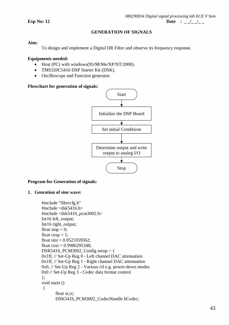
Flowchart for generation of signals:

Program for Generation of signals: 1. Genration of sine wave:

#include "filtercfg.h" #include <dsk5416.h> #include <dsk5416_pcm3002.h> Int16 left_output; Int16 right_output; float sinp = 0; float cosp = 1; float sini = 0.0523359562; float cosi = 0.9986295348; DSK5416_PCM3002_Config setup = 0x1ff, // Set-Up Reg 0 - Left channel DAC attenuation 0x1ff, // Set-Up Reg 1 - Right channel DAC attenuation 0x0, // Set-Up Reg 2 - Various ctl e.g. power-down modes 0x0 // Set-Up Reg 3 - Codec data format control ; void main ()

float st,ct; DSK5416_PCM3002_CodecHandle hCodec;

Start

Initialize the DSP Board

Set initial Conditions

Determine output and write output to analog I/O

Stop


44

// Initialize the board support library DSK5416_init(); // Start the codec hCodec = DSK5416_PCM3002_openCodec(0, &setup); // Set codec frequency DSK5416_PCM3002_setFreq(hCodec, 24000); // Endless loop IO audio codec while(1)

st = sinp*cosi + cosp*sini; ct = cosp*cosi - sinp*sini; sinp = st; cosp = ct; left_output=32768*sinp; right_output=left_output; // Write 16 bits to the codec, loop to retry if data port is busy while(!DSK5416_PCM3002_write16(hCodec, left_output)); while(!DSK5416_PCM3002_write16(hCodec, right_output));

2. Generation of Triangular wave:

#include "filtercfg.h" #include <dsk5416.h> #include <dsk5416_pcm3002.h> #define PI 3.14159265358979 Int16 left_output; Int16 right_output; float sinp[6] = 0,0,0,0,0,0; float cosp[6] = 1,1,1,1,1,1; float sini[6] = 0.0523359562, 0.1564344650, 0.2588190451, 0.3583679495, 0.4539904997, 0.5446390350; float cosi[6] = 0.9986295348, 0.9876883406, 0.9659258263, 0.9335804265, 0.8910065242, 0.8386705679; DSK5416_PCM3002_Config setup = 0x1ff, // Set-Up Reg 0 - Left channel DAC attenuation 0x1ff, // Set-Up Reg 1 - Right channel DAC attenuation 0x0, // Set-Up Reg 2 - Various ctl e.g. power-down modes 0x0 // Set-Up Reg 3 - Codec data format control ; void main ()

int j; float sp,cp,si,ci,st,ct,temp; DSK5416_PCM3002_CodecHandle hCodec; // Initialize the board support library DSK5416_init(); // Start the codec hCodec = DSK5416_PCM3002_openCodec(0, &setup); // Set codec frequency DSK5416_PCM3002_setFreq(hCodec, 24000); // Endless loop IO audio codec


45

while(1) for(j=0;j<6;j++)

sp = sinp[j]; cp = cosp[j]; si = sini[j]; ci = cosi[j]; st = sp*ci + cp*si; ct = cp*ci - sp*si; sinp[j] = st; cosp[j] = ct;

temp = 0.5; for(j=0;j<6;j++) temp += -4*cosp[j]/(PI*PI*(2*j+1)*(2*j+1));

left_output=32768*temp; right_output=left_output; // Write 16 bits to the codec, loop to retry if data port is busy while(!DSK5416_PCM3002_write16(hCodec, left_output)); while(!DSK5416_PCM3002_write16(hCodec, right_output));

Result:

Thus sine wave and triangular wave are generated using TMS320c5416 DSK.


46

Exp No: 13 Date : _ _/_ _/_ _

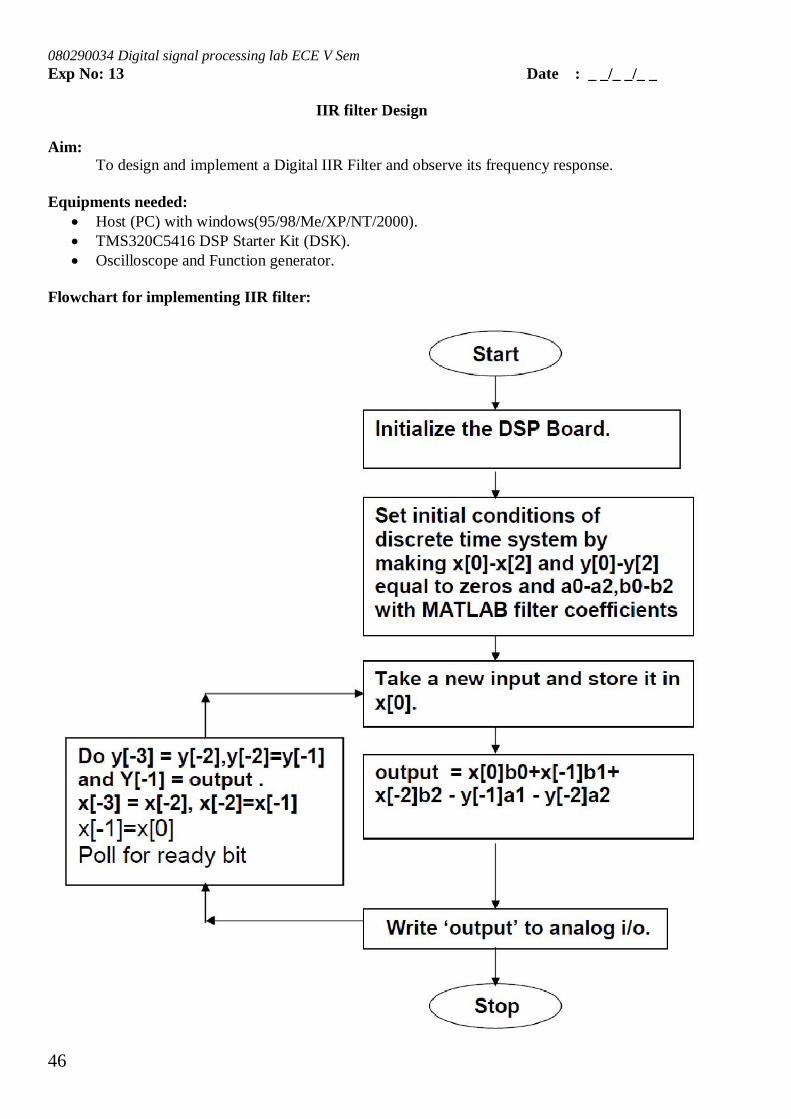
IIR filter Design Aim: To design and implement a Digital IIR Filter and observe its frequency response. Equipments needed:


Flowchart for implementing IIR filter:


47

‘C’ PROGRAM TO IMPLEMENT IIR FILTER: #include "filtercfg.h" #include <dsk5416.h> #include <dsk5416_pcm3002.h> Int16 left_input; Int16 left_output; Int16 right_input; Int16 right_output; const signed int filter_Coeff[ ] =48,48,48, 32767, -30949, 29322; DSK5416_PCM3002_Config setup = 0x1ff, // Set-Up Reg 0 - Left channel DAC attenuation 0x1ff, // Set-Up Reg 1 - Right channel DAC attenuation 0x0, // Set-Up Reg 2 - Various ctl e.g. power-down modes 0x0 // Set-Up Reg 3 - Codec data format control ; void main ()

DSK5416_PCM3002_CodecHandle hCodec; // Initialize the board support library DSK5416_init(); // Start the codec hCodec = DSK5416_PCM3002_openCodec(0, &setup); // Set codec frequency DSK5416_PCM3002_setFreq(hCodec,24000); // Endless loop IO audio codec while(1) // Read 16 bits of codec data, loop to retry if data port is busy while(!DSK5416_PCM3002_read16(hCodec, &left_input)); while(!DSK5416_PCM3002_read16(hCodec, &right_input)); left_output=IIR_FILTER(&filter_Coeff , left_input); right_output=left_output; // Write 16 bits to the codec, loop to retry if data port is busy while(!DSK5416_PCM3002_write16(hCodec, left_output)); while(!DSK5416_PCM3002_write16(hCodec, right_output));

signed int IIR_FILTER(const signed int * h, signed int x1)

static signed int x[6] = 0, 0, 0, 0, 0, 0 ; /* x(n), x(n-1), x(n-2). Must be static */ static signed int y[6] = 0, 0, 0, 0, 0, 0 ; /* y(n), y(n-1), y(n-2). Must be static */ long temp=0; temp = x1; /* Copy input to temp */ x[0] = (signed int) temp; /* Copy input to x[stages][0] */ temp = ( (long)h[0] * x[0]) ; /* B0 * x(n) */ temp += ( (long)h[1] * x[1]); /* B1/2 * x(n-1) */ temp += ( (long)h[1] * x[1]); /* B1/2 * x(n-1) */ temp += ( (long)h[2] * x[2]); /* B2 * x(n-2) */ temp -= ( (long)h[4] * y[1]); /* A1/2 * y(n-1) */


48

temp -= ( (long)h[4] * y[1]); /* A1/2 * y(n-1) */ temp -= ( (long)h[5] * y[2]); /* A2 * y(n-2) */ /* Divide temp by coefficients[A0] */ temp >>= 15; if ( temp > 32767 ) temp = 32767; else if ( temp < -32767) temp = -32767; y[0] = (short int) ( temp ); /* Shuffle values along one place for next time */ y[2] = y[1]; /* y(n-2) = y(n-1) */ y[1] = y[0]; /* y(n-1) = y(n) */ x[2] = x[1]; /* x(n-2) = x(n-1) */ x[1] = x[0]; /* x(n-1) = x(n) */ /* temp is used as input next time through */ return ((short int)temp*1);


49

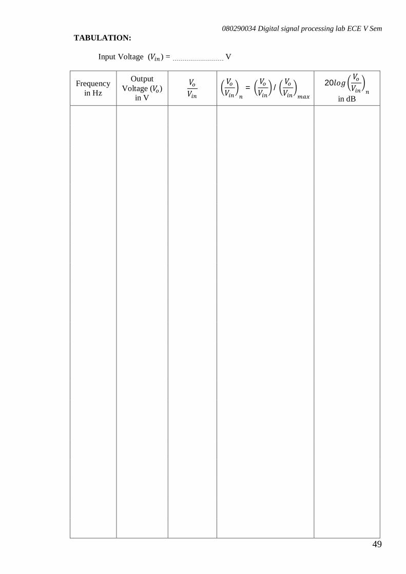
TABULATION:

Input Voltage (푉 ) = V

Frequency in Hz

Output Voltage (푉 )

in V

푉푉

푉푉 =

푉푉 /

푉푉 20푙표푔

푉푉

in dB


50

Procedure:

Switch on the DSP board. Open the Code Composer Studio. Create a new project Project " New (File Name. pjt , Eg: Filter.pjt) Initialize the McBSP, the DSP board and the on board codec.

“Kindly refer the Topic Configuration of 5416 McBSP using CSL” Add the given above .C. source file to the current project(remove mcbsp_io.c source

file from the project if you have already added). Connect the speaker jack to the input of the CRO. Build the program. Load the generated object file(*.out) on to Target board. Run the program using F5. Observe the waveform that appears on the CRO screen.

Result:

Thus a Digital IIR Filter is designed and implemented and its frequency response is observed.


51

Exp No: 14 Date : _ _/_ _/_ _

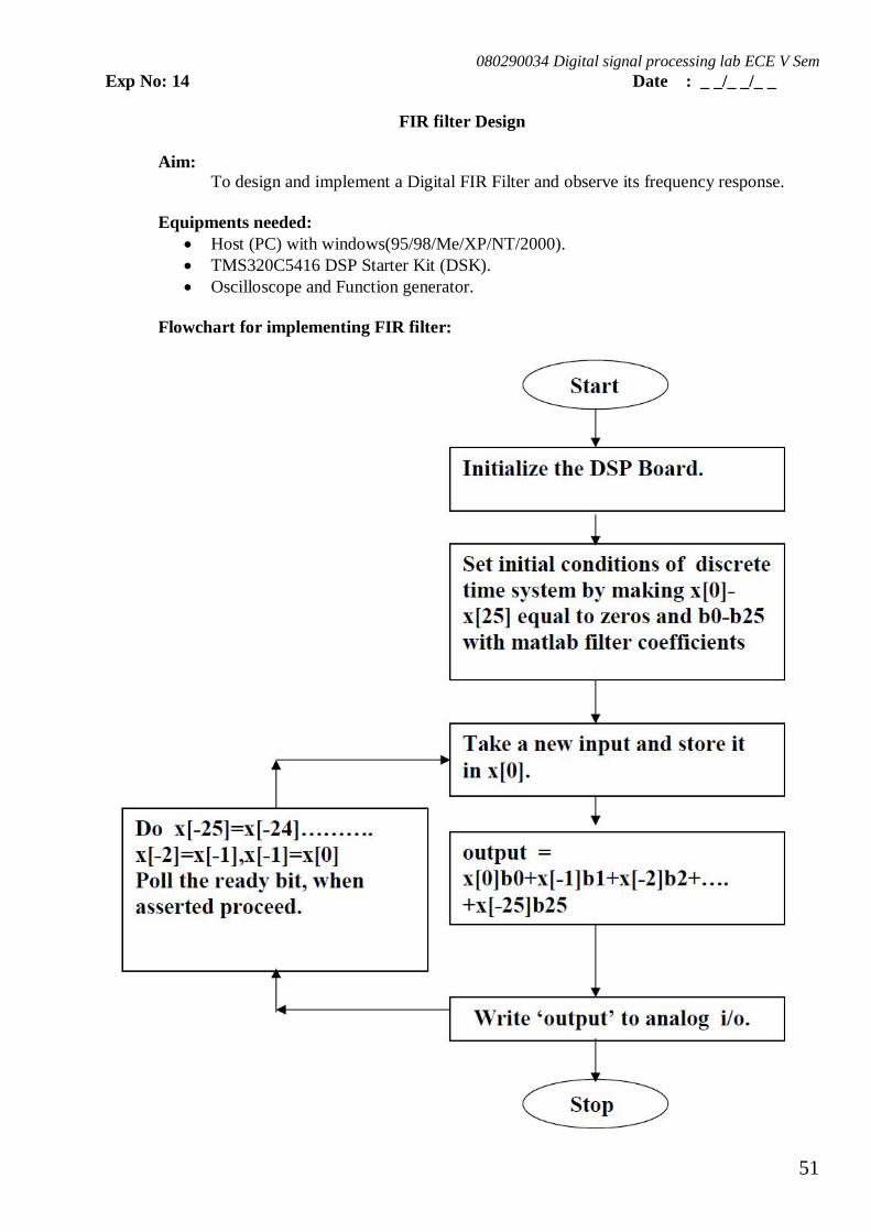
FIR filter Design

Aim: To design and implement a Digital FIR Filter and observe its frequency response.

Equipments needed:


Flowchart for implementing FIR filter:


52

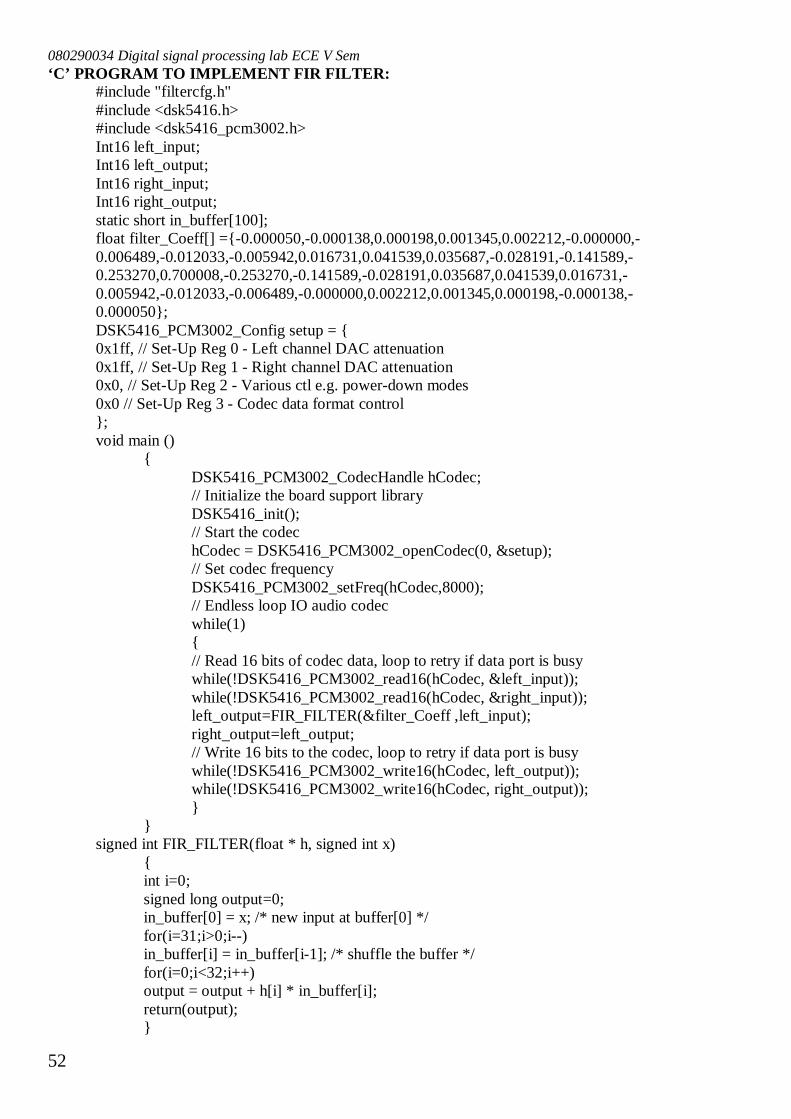
‘C’ PROGRAM TO IMPLEMENT FIR FILTER: #include "filtercfg.h" #include <dsk5416.h> #include <dsk5416_pcm3002.h> Int16 left_input; Int16 left_output; Int16 right_input; Int16 right_output; static short in_buffer[100]; float filter_Coeff[] =-0.000050,-0.000138,0.000198,0.001345,0.002212,-0.000000,-0.006489,-0.012033,-0.005942,0.016731,0.041539,0.035687,-0.028191,-0.141589,-0.253270,0.700008,-0.253270,-0.141589,-0.028191,0.035687,0.041539,0.016731,-0.005942,-0.012033,-0.006489,-0.000000,0.002212,0.001345,0.000198,-0.000138,-0.000050; DSK5416_PCM3002_Config setup = 0x1ff, // Set-Up Reg 0 - Left channel DAC attenuation 0x1ff, // Set-Up Reg 1 - Right channel DAC attenuation 0x0, // Set-Up Reg 2 - Various ctl e.g. power-down modes 0x0 // Set-Up Reg 3 - Codec data format control ; void main ()

DSK5416_PCM3002_CodecHandle hCodec; // Initialize the board support library DSK5416_init(); // Start the codec hCodec = DSK5416_PCM3002_openCodec(0, &setup); // Set codec frequency DSK5416_PCM3002_setFreq(hCodec,8000); // Endless loop IO audio codec while(1) // Read 16 bits of codec data, loop to retry if data port is busy while(!DSK5416_PCM3002_read16(hCodec, &left_input)); while(!DSK5416_PCM3002_read16(hCodec, &right_input)); left_output=FIR_FILTER(&filter_Coeff ,left_input); right_output=left_output; // Write 16 bits to the codec, loop to retry if data port is busy while(!DSK5416_PCM3002_write16(hCodec, left_output)); while(!DSK5416_PCM3002_write16(hCodec, right_output));

signed int FIR_FILTER(float * h, signed int x)

int i=0; signed long output=0; in_buffer[0] = x; /* new input at buffer[0] */ for(i=31;i>0;i--) in_buffer[i] = in_buffer[i-1]; /* shuffle the buffer */ for(i=0;i<32;i++) output = output + h[i] * in_buffer[i]; return(output);


53

TABULATION:

Input Voltage (푉 ) = V

Frequency in Hz

Output Voltage (푉 )

in V

푉푉

푉푉 =

푉푉 /

푉푉 20푙표푔

푉푉

in dB


54

Procedure:

Switch on the DSP board. Open the Code Composer Studio. Create a new project Project " New (File Name. pjt , Eg: Filter.pjt) Initialize the McBSP, the DSP board and the on board codec.

“Kindly refer the Topic Configuration of 5416 McBSP using CSL” Add the given above .C. source file to the current project(remove mcbsp_io.c source

file from the project if you have already added). Connect the speaker jack to the input of the CRO. Build the program. Load the generated object file(*.out) on to Target board. Run the program using F5. Observe the waveform that appears on the CRO screen.

Result:

Thus a Digital FIR Filter is designed and implemented and its frequency response is observed.