Practical Implementation of FACTs On A Model Transmission Line For Performance

Improvement

Supervised By:

Prof. Dr. Muhammad Fayyaz Khan

United International University (UIU)

Presented By:Saifur Rahman 021 111 056MD.Rakib Mohan 021 111 004Mohammad Shakhawat Hossain 021 111 117MD.Jabaidur Rahman 021 101 107

CONTENTS

What is FACTs?

Objectives of FACTs

Types of FACTS Controllers

Transmission line Parameters & Design of FACTS Controllers

Advantages of FACTS Controllers

Conclusion

Reference

What is FACTs?

FACTs is an acronym for Flexible AC Transmission Systems. FACTS uses solid state switching devices to control power flow through a transmission network , So that the transmission network is loaded to its full capacity.

FACTs idea was put forward by Prof. Hingorani of EPRI, USA in 1988 .

A line can be loaded up to its full thermal limit by FACTs.

Power transfer can be increased thru an old line by FACTs.

History Of FACTs Flexible AC Transmission Systems Technology (FACTS)

was first proposed by the Dr Narain G. Hingorani in 1988 of Electric Power Research Institute ( EPRI ), USA .

The first FACTS installation was at the C. J. Slatt Substation near Arlington, Oregon.

This is a 500 kV, 3-phase 60 Hz substation, and was developed by EPRI, the Bonneville Power Administration and General Electric Company.

C. J. Slatt Substation near Arlington, Oregon., USA(Google Map view)

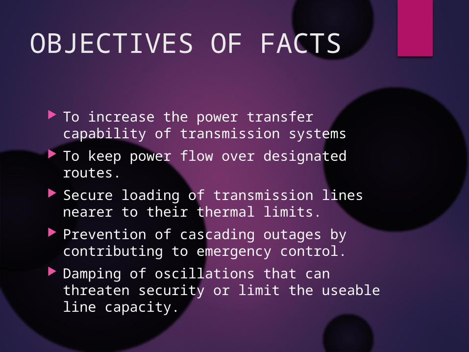
OBJECTIVES OF FACTS

To increase the power transfer capability of transmission systems

To keep power flow over designated routes.

Secure loading of transmission lines nearer to their thermal limits.

Prevention of cascading outages by contributing to emergency control.

Damping of oscillations that can threaten security or limit the useable line capacity.

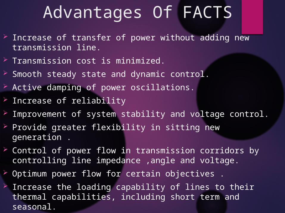
Advantages Of FACTS Increase of transfer of power without adding new transmission line.

Transmission cost is minimized.

Smooth steady state and dynamic control.

Active damping of power oscillations.

Increase of reliability

Improvement of system stability and voltage control.

Provide greater flexibility in sitting new generation .

Control of power flow in transmission corridors by controlling line impedance ,angle and voltage.

Optimum power flow for certain objectives .

Increase the loading capability of lines to their thermal capabilities, including short term and seasonal.

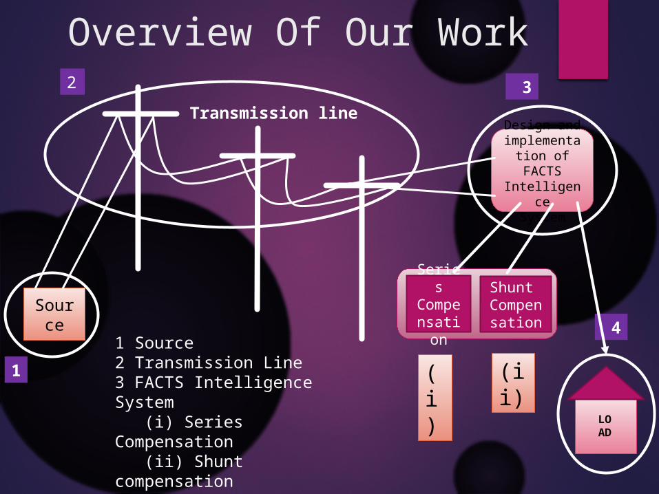
Overview Of Our Work

Source

Transmission line

LOAD

1

3

41 Source2 Transmission Line 3 FACTS Intelligence System (i) Series Compensation (ii) Shunt compensation4 Load

Design and implementation

of FACTSIntelligence

System

2

SeriesCompensation

Shunt Compens

ation

(i)

(ii)

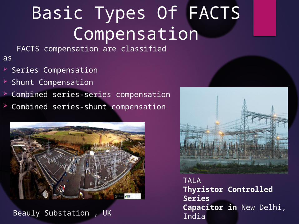
Basic Types Of FACTS Compensation

FACTS compensation are classified as

Series Compensation

Shunt Compensation

Combined series-series compensation

Combined series-shunt compensation

TALAThyristor Controlled SeriesCapacitor in New Delhi, India

Beauly Substation , UK

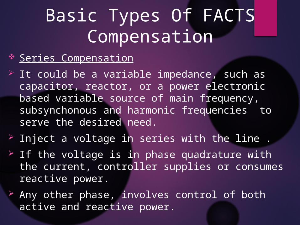
Basic Types Of FACTS Compensation

Series Compensation

It could be a variable impedance, such as capacitor, reactor, or a power electronic based variable source of main frequency, subsynchonous and harmonic frequencies to serve the desired need.

Inject a voltage in series with the line .

If the voltage is in phase quadrature with the current, controller supplies or consumes reactive power.

Any other phase, involves control of both active and reactive power.

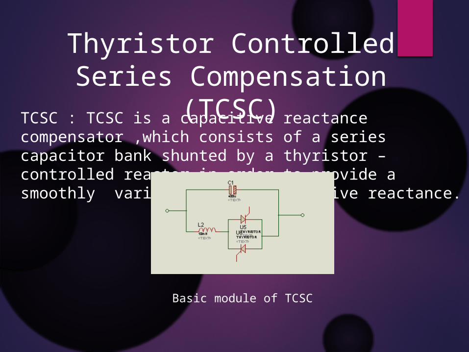
Thyristor Controlled Series Compensation (TCSC)

TCSC : TCSC is a capacitive reactance compensator ,which consists of a series capacitor bank shunted by a thyristor – controlled reactor in order to provide a smoothly variable series capacitive reactance.

Basic module of TCSC

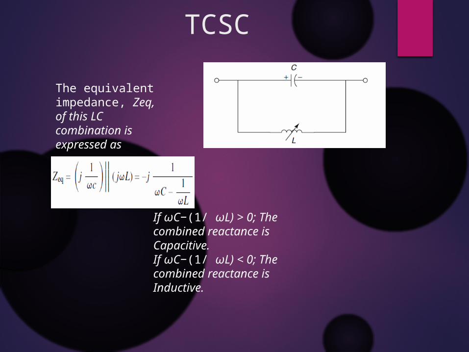
TCSC

The equivalent impedance, Zeq, of this LC combination is expressed as

If ωC−(1/ ωL) > 0; The combined reactance is Capacitive. If ωC−(1/ ωL) < 0; The combined reactance is Inductive.

Benefits of TCSC

Current control

Damping Oscillations

Transient and Dynamic stability

Voltage stability

Fault current limiting

Basic Types Of FACTS Compensation

Shunt compensation

It could be a variable impedance (capacitor ,reactor , etc.) or a power electronic based variable source or combination of both .

Inject a current in the system.

If the current is in phase quadrature with the voltage ,controller supplies or consumes reactive power.

Any other phase ,involves control of both active and reactive power.

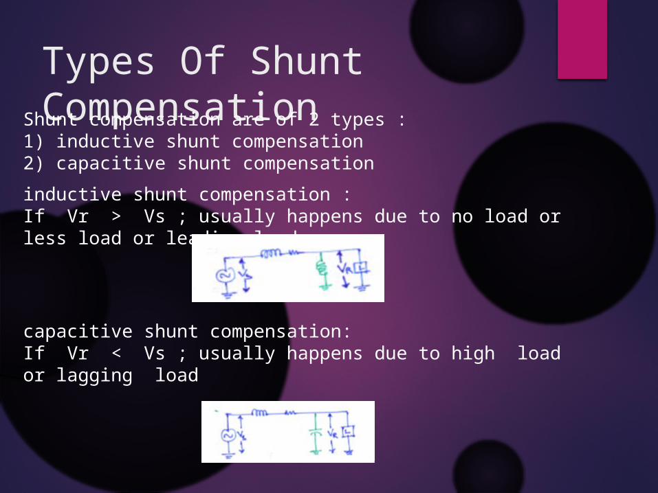
Types Of Shunt CompensationShunt compensation are of 2 types :1) inductive shunt compensation 2) capacitive shunt compensation

inductive shunt compensation :If Vr > Vs ; usually happens due to no load or less load or leading load

capacitive shunt compensation: If Vr < Vs ; usually happens due to high load or lagging load

FACTs Implemented On a Model Transmission Line (Theoretical)

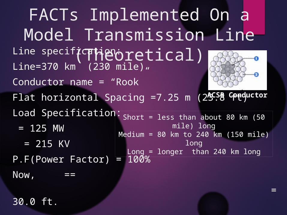
Line specification:

Line=370 km (230 mile)

Conductor name = “Rook”

Flat horizontal Spacing =7.25 m (23.8 ft)

Load Specification:

= 125 MW

= 215 KV

P.F(Power Factor) = 100%

Now, ==

= 30.0 ft.

 

ACSR Conductor

Short = less than about 80 km (50 mile) longMedium = 80 km to 240 km (150 mile) long

Long = longer than 240 km long

1 2 3

2 * 23.8

23.8 23.8

FACTs Implemented On a Model Transmission Line (Theoretical)

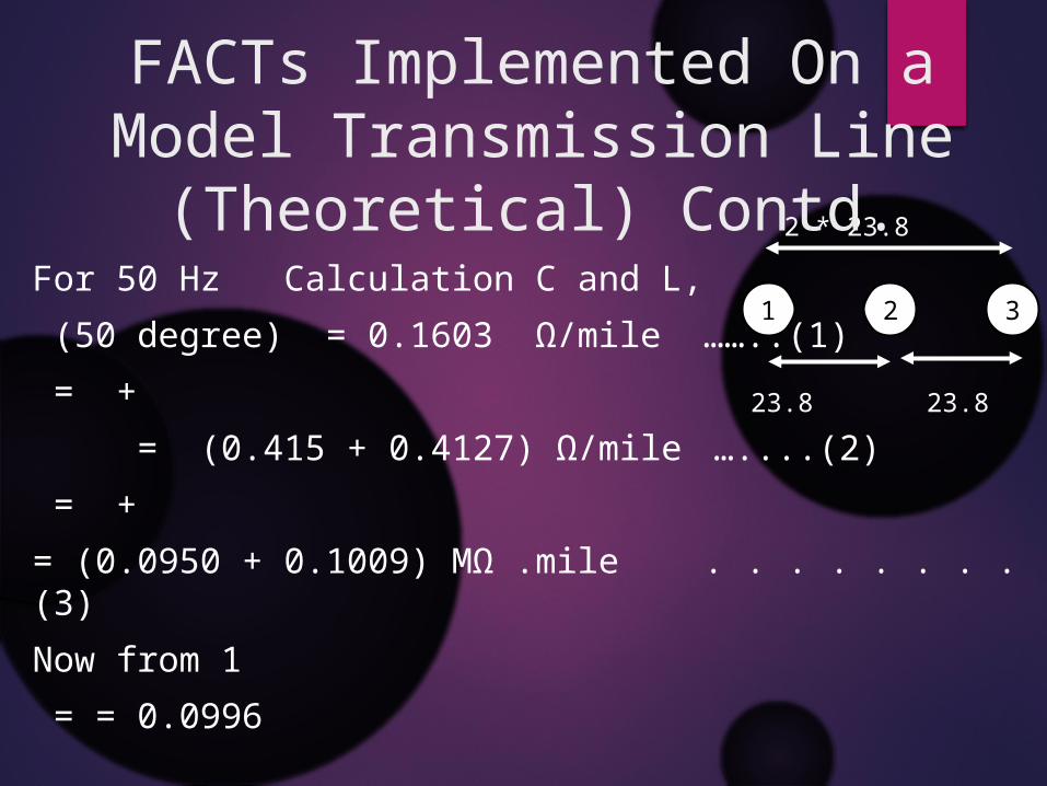
Contd.For 50 Hz Calculation C and L,

(50 degree) = 0.1603 Ω/mile ……..(1)

= +

= (0.415 + 0.4127) Ω/mile …....(2)

= +

= (0.0950 + 0.1009) MΩ .mile . . . . . . . .(3)

Now from 1

= = 0.0996

FACTs Implemented On a Model Transmission Line (Theoretical)

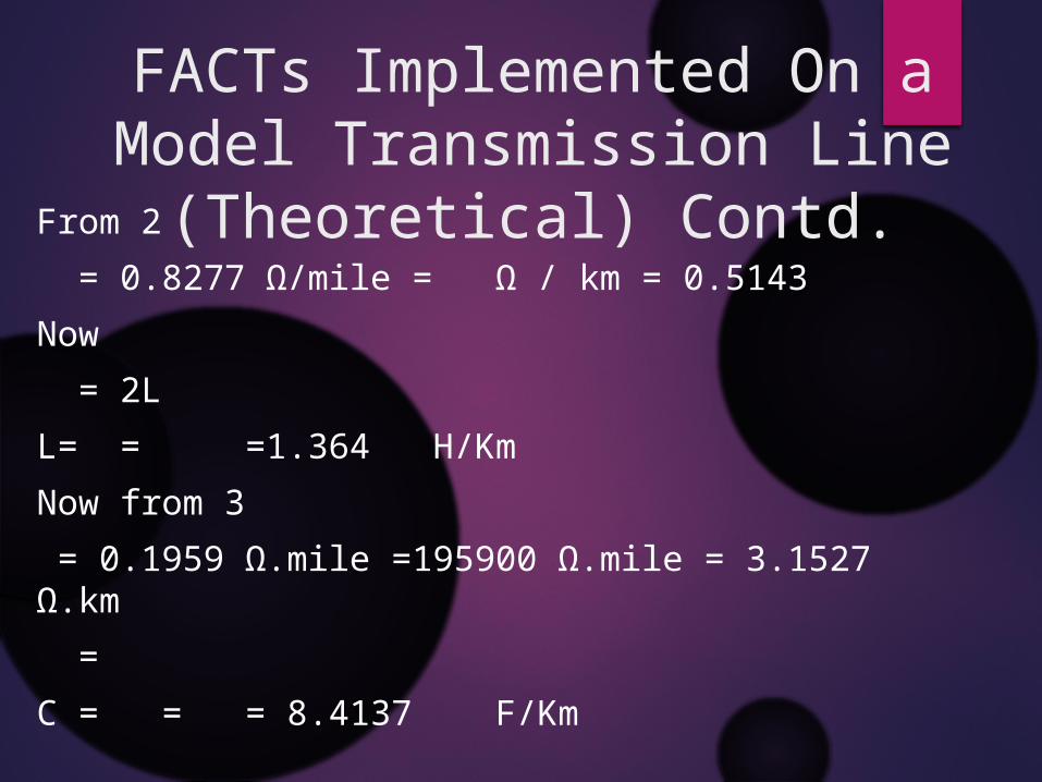
Contd.From 2

= 0.8277 Ω/mile = Ω / km = 0.5143

Now

= 2L

L= = =1.364 H/Km

Now from 3

= 0.1959 Ω.mile =195900 Ω.mile = 3.1527 Ω.km

  =

C = = = 8.4137 F/Km

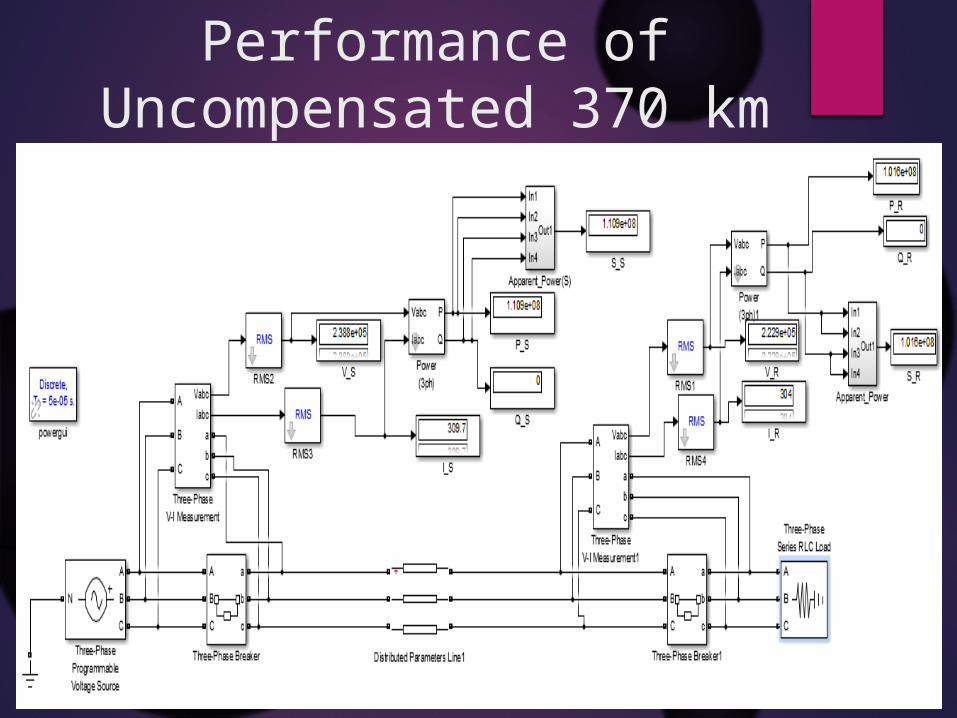
Performance of Uncompensated 370 km line with Resistive Load

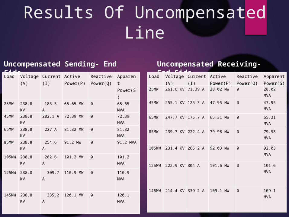
Results Of Uncompensated Line

Load Voltage(V)

Current(I)

Active Power(P)

Reactive Power(Q)

Apparent Power(S)

25MW 238.8 KV 183.3 A 65.65 MW 0 65.65 MVA

45MW 238.8 KV 202.1 A 72.39 MW 0 72.39 MVA

65MW 238.8 KV 227 A 81.32 MW 0 81.32 MVA

85MW 238.8 KV 254.6 A 91.2 MW 0 91.2 MVA

105MW

238.8 KV 282.6 A 101.2 MW 0 101.2 MVA

125MW

238.8 KV 309.7 A 110.9 MW 0 110.9 MVA

145MW

238.8 KV 335.2 A 120.1 MW 0 120.1 MVA

Uncompensated Sending- End Side Uncompensated Receiving- End Side

Load Voltage(V)

Current(I)

Active Power(P)

Reactive Power(Q)

Apparent Power(S)

25MW 261.6 KV 71.39 A 28.02 MW 0 28.02 MVA

45MW 255.1 KV 125.3 A 47.95 MW 0 47.95 MVA

65MW 247.7 KV 175.7 A 65.31 MW 0 65.31 MVA

85MW 239.7 KV 222.4 A 79.98 MW 0 79.98 MVA

105MW

231.4 KV 265.2 A 92.03 MW 0 92.03 MVA

125MW

222.9 KV 304 A 101.6 MW 0 101.6 MVA

145MW

214.4 KV 339.2 A 109.1 MW 0 109.1 MVA

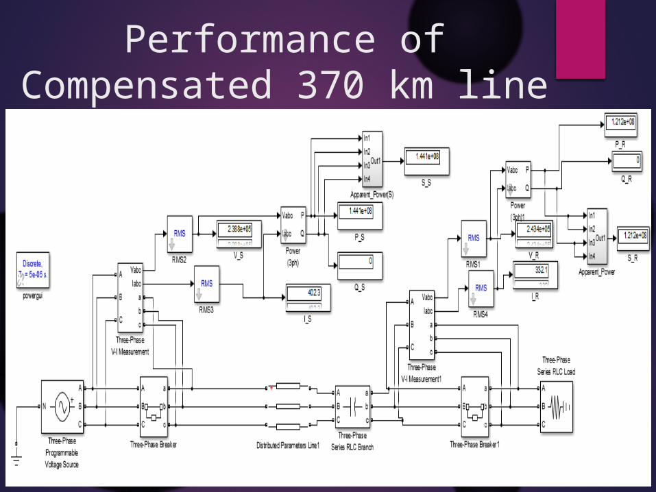
Performance of Compensated 370 km line with Resistive Load

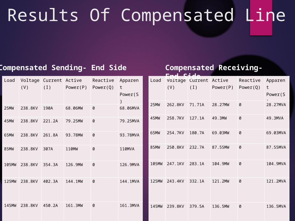
Results Of Compensated Line

Load Voltage(V)

Current(I)

Active Power(P)

Reactive Power(Q)

Apparent Power(S)

25MW 238.8KV 190A 68.06MW 0 68.06MVA

45MW 238.8KV 221.2A 79.25MW 0 79.25MVA

65MW 238.8KV 261.8A 93.78MW 0 93.78MVA

85MW 238.8KV 307A 110MW 0 110MVA

105MW

238.8KV 354.3A 126.9MW 0 126.9MVA

125MW

238.8KV 402.3A 144.1MW 0 144.1MVA

145MW

238.8KV 450.2A 161.3MW 0 161.3MVA

Compensated Sending- End Side

Load Voltage(V)

Current(I)

Active Power(P)

Reactive Power(Q)

Apparent Power(S)

25MW 262.8KV 71.71A 28.27MW 0 28.27MVA

45MW 258.7KV 127.1A 49.3MW 0 49.3MVA

65MW 254.7KV 180.7A 69.03MW 0 69.03MVA

85MW 250.8KV 232.7A 87.55MW 0 87.55MVA

105MW

247.1KV 283.1A 104.9MW 0 104.9MVA

125MW

243.4KV 332.1A 121.2MW 0 121.2MVA

145MW

239.8KV 379.5A 136.5MW 0 136.5MVA

Compensated Receiving- End Side

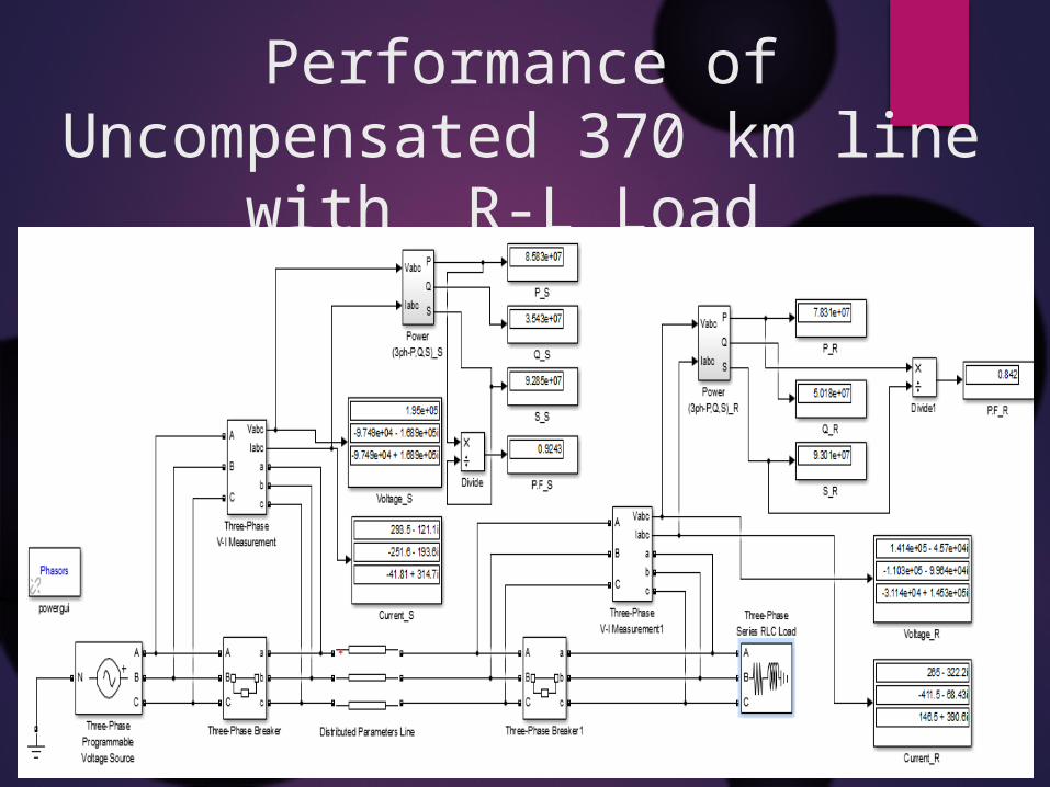
Performance of Uncompensated 370 km line with R-L Load

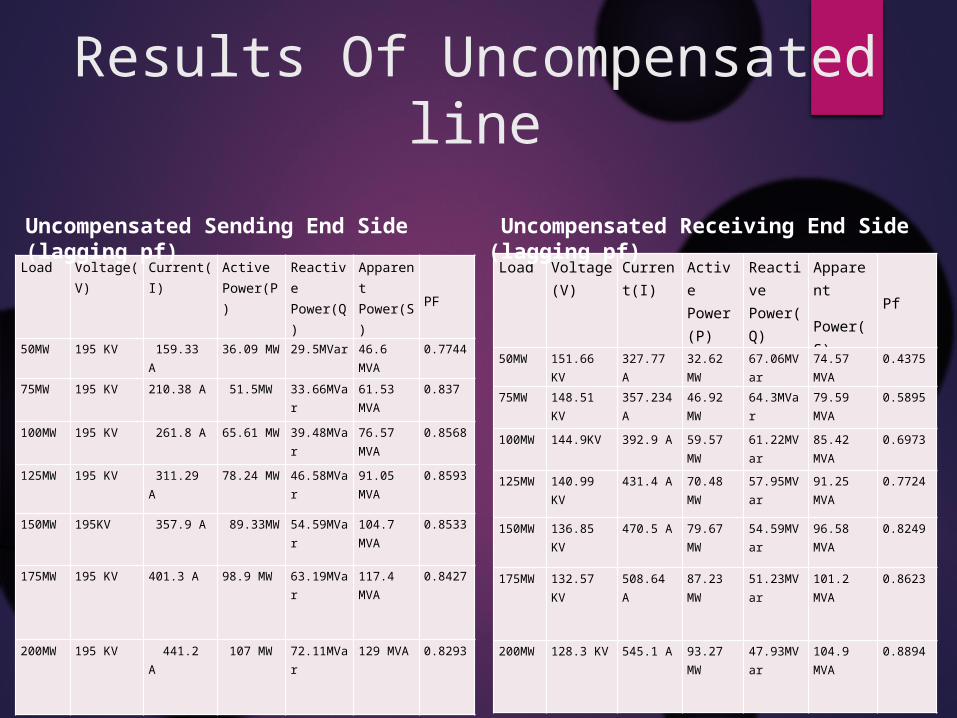
Results Of Uncompensated line

Load Voltage(V)

Current(I) Active Power(P)

Reactive Power(Q)

Apparent Power(S)

 

PF

50MW 195 KV 159.33 A 36.09 MW

29.5MVar 46.6 MVA

0.7744

75MW 195 KV 210.38 A 51.5MW 33.66MVar

61.53 MVA

0.837

100MW

195 KV 261.8 A 65.61 MW

39.48MVar

76.57 MVA

0.8568

125MW

195 KV 311.29 A 78.24 MW

46.58MVar

91.05 MVA

0.8593

150MW

195KV 357.9 A 89.33MW

54.59MVar

104.7 MVA

0.8533

175MW

195 KV 401.3 A 98.9 MW 63.19MVar

117.4 MVA

0.8427

200MW

195 KV 441.2 A 107 MW 72.11MVar

129 MVA 0.8293

Uncompensated Sending End Side (lagging pf)

Load Voltage(V)

Current(I)

Active Power(P)

Reactive Power(Q)

Apparent

Power(S)

 

Pf

50MW 151.66 KV

327.77 A 32.62 MW

67.06MVar

74.57 MVA

0.4375

75MW 148.51 KV

357.234 A

46.92 MW

64.3MVar

79.59 MVA

0.5895

100MW

144.9KV 392.9 A 59.57 MW

61.22MVar

85.42 MVA

0.6973

125MW

140.99 KV

431.4 A 70.48 MW

57.95MVar

91.25 MVA

0.7724

150MW

136.85 KV

470.5 A 79.67 MW

54.59MVar

96.58 MVA

0.8249

175MW

132.57 KV

508.64 A 87.23 MW

51.23MVar

101.2 MVA

0.8623

200MW

128.3 KV 545.1 A 93.27 MW

47.93MVar

104.9 MVA

0.8894

Uncompensated Receiving End Side (lagging pf)

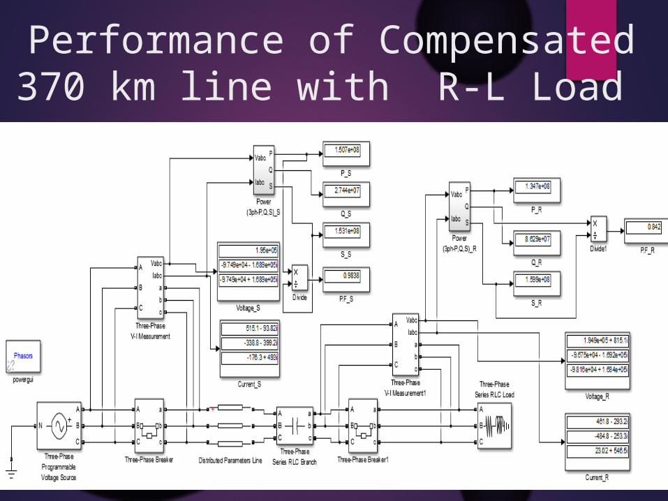
Performance of Compensated 370 km line with R-L Load

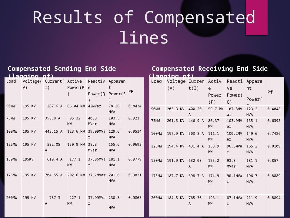
Results of Compensated lines

Load Voltage(V)

Current(I) Active Power(P)

Reactive Power(Q)

Apparent Power(S)

 

PF

50MW 195 KV 267.6 A 66.04 MW

42MVar 78.26 MVA

0.8434

75MW 195 KV 353.8 A 95.32 MW

40.3 MVar

103.5 MVA

0.921

100MW

195 KV 443.15 A 123.6 MW

39.09MVar

129.6 MVA

0.9534

125MW

195 KV 532.05 A 150.8 MW

38.3 MVar

155.6 MVA

0.9693

150MW

195KV 619.4 A 177.1 MW

37.86MVar

181.1 MVA

0.9779

175MW

195 KV 704.55 A 202.6 MW

37.7MVar 201.6 MVA

0.9831

200MW

195 KV 787.3 A 227.1 MW

37.99MVar

230.3

MVA

0.9863

Compensated Sending End Side (lagging pf)

Load Voltage(V)

Current(I)

Active Power(P)

Reactive Power(Q)

Apparent

Power(S)

 

Pf

50MW 205.3 KV 400.20 A 59.7 MW

107.8MVar

123.2 MVA

0.4848

75MW 201.5 KV 446.9 A 86.37 MW

103.9MVar

135.1 MVA

0.6393

100MW

197.9 KV 503.8 A 111.1 MW

100.2MVar

149.6 MVA

0.7426

125MW

194.4 KV 431.4 A 133.9 MW

96.6MVar

165.2 MVA

0.8109

150MW

191.9 KV 632.03 A 155.2 MW

93.3 MVar

181.1 MVA

0.857

175MW

187.7 KV 698.7 A 174.9 MW

90.1MVar

196.7 MVA

0.8889

200MW

184.5 KV 765.36 A 193.1 MW

87.1MVar

211.9 MVA

0.8894

Compensated Receiving End Side (lagging pf)

FACTs Implemented On a Model Transmission Line (practical)

A single phase 2 Km line was taken for FACTs application and implementation in the lab.

Line parameters are calculated

Line performance was simulated under different load conditions

FACTs controller was designed to improve the line performance

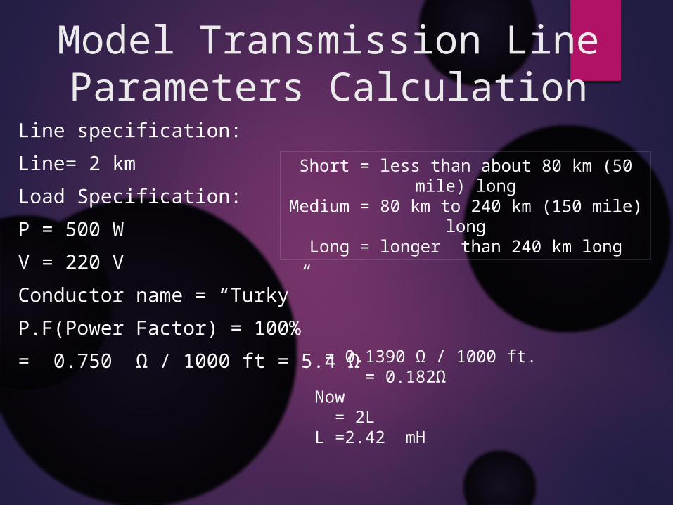
Model Transmission Line Parameters Calculation

Line specification:

Line= 2 km

Load Specification:

P = 500 W

V = 220 V

Conductor name = “Turky”

P.F(Power Factor) = 100%

= 0.750 Ω / 1000 ft = 5.4 Ω

Short = less than about 80 km (50 mile) longMedium = 80 km to 240 km (150 mile) long

Long = longer than 240 km long

= 0.1390 Ω / 1000 ft. = 0.182Ω Now = 2LL =2.42 mH

Source220 V50 Hz

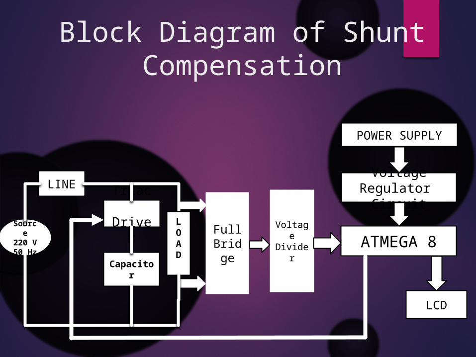
Block Diagram of Shunt Compensation

LINE

LOAD

FullBridge

Voltage Divider

POWER SUPPLY

Voltage Regulator Circuit

ATMEGA 8

LCD

Capacitor

Triac Driver

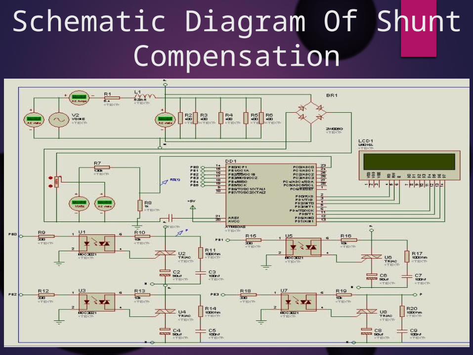
Schematic Diagram Of Shunt Compensation

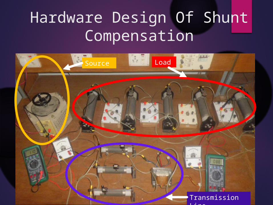
Hardware Design Of Shunt Compensation

Load

Transmission Line

Source

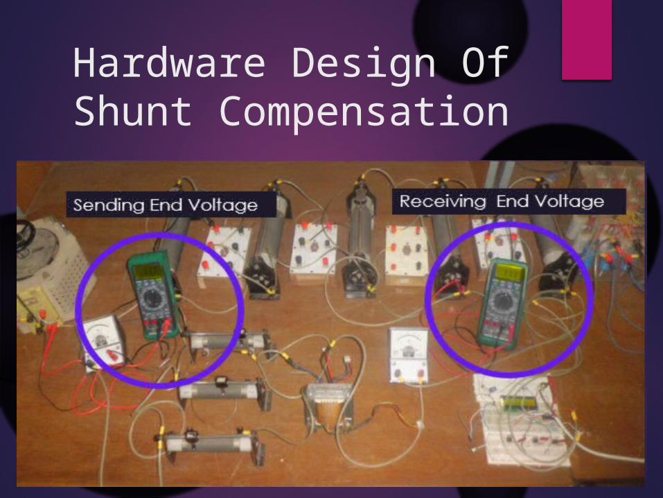
Hardware Design Of Shunt Compensation

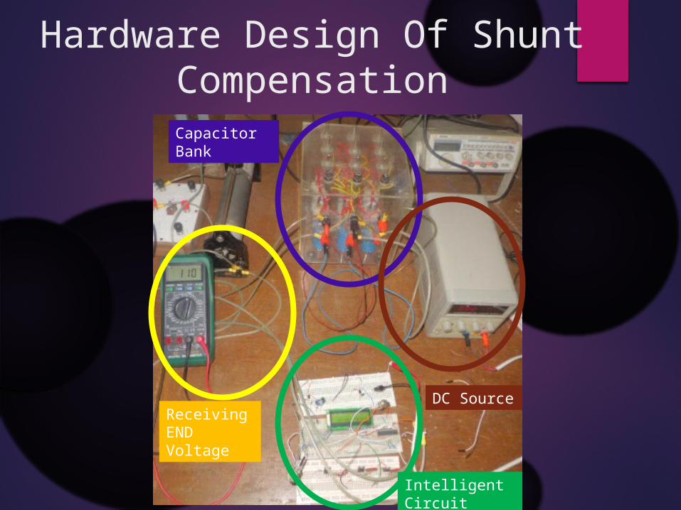
Hardware Design Of Shunt Compensation

Receiving END Voltage

Capacitor Bank

DC Source

Intelligent Circuit

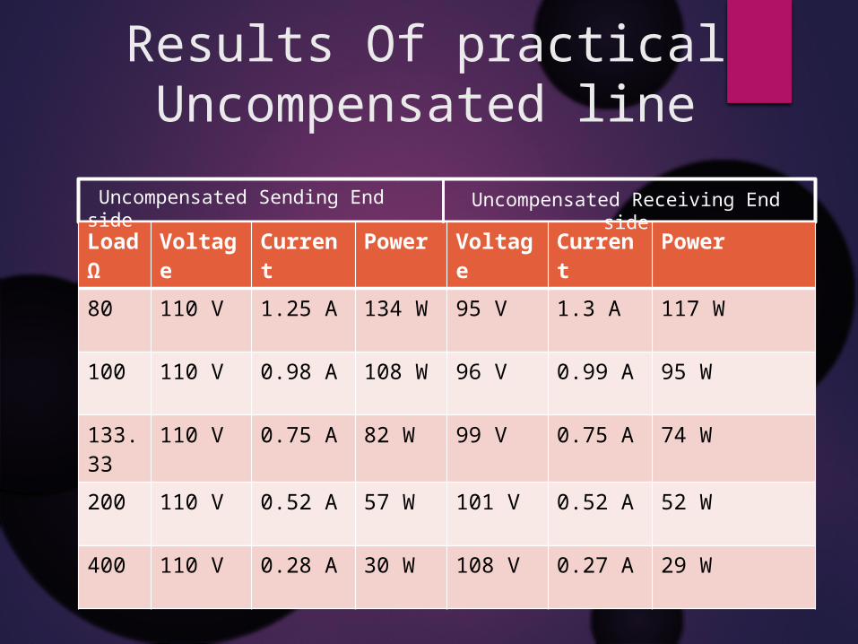
Results Of practical Uncompensated line

LoadΩ

Voltage

Current

Power

Voltage

Current

Power

80 110 V 1.25 A 134 W 95 V 1.3 A 117 W

100 110 V 0.98 A 108 W 96 V 0.99 A 95 W

133.33

110 V 0.75 A 82 W 99 V 0.75 A 74 W

200 110 V 0.52 A 57 W 101 V 0.52 A 52 W

400 110 V 0.28 A 30 W 108 V 0.27 A 29 W

Uncompensated Sending End side Uncompensated Receiving End side

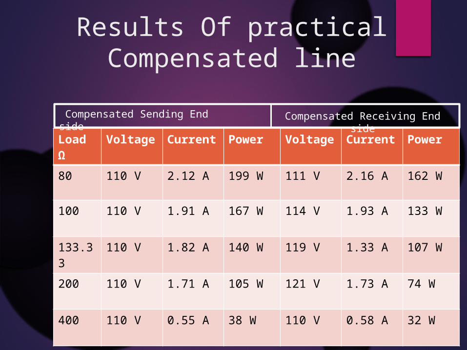
Results Of practical Compensated line

LoadΩ

Voltage Current Power Voltage Current Power

80 110 V 2.12 A 199 W 111 V 2.16 A 162 W

100 110 V 1.91 A 167 W 114 V 1.93 A 133 W

133.33

110 V 1.82 A 140 W 119 V 1.33 A 107 W

200 110 V 1.71 A 105 W 121 V 1.73 A 74 W

400 110 V 0.55 A 38 W 110 V 0.58 A 32 W

Compensated Sending End side Compensated Receiving End side

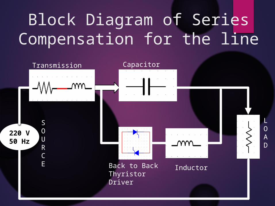
Block Diagram of Series Compensation for the line

220 V50 Hz

Transmission Line Capacitor

LOAD

SOURCE Back to Back

Thyristor DriverInductor

Block Diagram of Series Compensation in the Matlab

Simulink

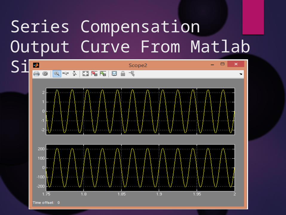
Series Compensation Output Curve From Matlab Simulink

Future Work

1. Simulation of different heavily loaded transmission line from FACTS. e.g East West Interconnector.

2. Measurement of stability and reliability study of Power sector of Bangladesh from FACTS .

Conclusion

We see that in an uncompensated line, the output voltage is less than the input voltage for the reason of transmission line parameters. After adding shunt compensation with the line we saw that the output voltage is improved. As well as after adding series compensation with the line the output voltage is also improved. If we implement this FACTS Controller in our transmission line network, economically it will beneficial for us.

Reference

•Hingorani, N.G., "Power Electronics in Electric Utilities:Role of Power Electronics in Future Power Systems,"Proceedings of the IEEE Special Issue Vol. 76, no. 4, April1988.•Thyristor-Based Facts Controllers For Electrical Ttransmission Systems by R. Mohan Mathur and Rajiv K. Varma•http://www.energy.siemens.com/co/pool/hq/power-transmission/FACTS/FACTS_Series_Compensation_neues%20CD.pdf• www.siemens.com/energy/facts•http://www.iosrjen.org/Papers/vol3_issue4%20(part-1)/C03411726.pdf•http://www.onsemi.com/pub_link/Collateral/HBD855-D.PDF

Any Question?

Thank You