Download pdf - An intercomparison and verification of outputs of several climate models on representative Mediterranean catchments

Hydrol. Earth Syst. Sci., 17, 1–19, 2013www.hydrol-earth-syst-sci.net/17/1/2013/doi:10.5194/hess-17-1-2013© Author(s) 2013. CC Attribution 3.0 License.

Hydrology and Earth System

SciencesO

pen Access

Regional climate models’ performance in representing precipitationand temperature over selected Mediterranean areas

R. Deidda1,3, M. Marrocu 2, G. Caroletti1,3,6, G. Pusceddu2, A. Langousis7, V. Lucarini 1,5, M. Puliga1,3, andA. Speranza1,4

1CINFAI, Consorzio Interuniversitario Nazionale per la Fisica delle Atmosfere e delle Idrosfere, Camerino, MC, Italy2CRS4, Centro di Ricerca, Sviluppo e Studi Superiori in Sardegna, Loc. Piscina Manna, Edificio 1, 09010 Pula, CA, Italy3Dipartimento di Ingegneria Civile, Ambientale e Architettura, Università di Cagliari, Piazza d’Armi, 09123 Cagliari, Italy4Dipartimento di Fisica, Università di Camerino, Via Madonna delle Carceri 9, Camerino, MC, Italy5Klimacampus, Institute of Meteorology, University of Hamburg, Hamburg, Germany6Bjerknes Center for Climate Research and Geophysical Institute, University of Bergen, Bergen, Norway7Department of Civil Engineering, University of Patras, Patras, Greece

Correspondence to:R. Deidda ([email protected])

Received: 19 June 2013 – Published in Hydrol. Earth Syst. Sci. Discuss.: 11 July 2013Revised: 4 November 2013 – Accepted: 9 November 2013 – Published:

Abstract. This paper discusses the relative performance ofseveral climate models in providing reliable forcing for hy-drological modeling in six representative catchments in theMediterranean region. We consider 14 Regional ClimateModels (RCMs), from the EU-FP6 ENSEMBLES project,run for the A1B emission scenario on a common 0.22◦

(about 24 km) rotated grid over Europe and the Mediter-ranean regionCE1. In the validation period (1951 to 2010) weconsider daily precipitation and surface temperatures fromthe observed data fields (E-OBS) data set, available from theENSEMBLES project and the data providers in the ECA&Dproject. Our primary objective is to rank the 14 RCMs foreach catchment and select the four best-performing onesto use as common forcing for hydrological models in thesix Mediterranean basins considered in the EU-FP7 CLIMBproject. Using a common suite of four RCMs for all studiedcatchments reduces the (epistemic) uncertainty when eval-uating trends and climate change impacts in the 21st cen-tury. We present and discuss the validation setting, as wellas the obtained results and, in some detail, the difficultieswe experienced when processing the data. In doing so wealso provide useful information and advice for researchersnot directly involved in climate modeling, but interested inthe use of climate model outputs for hydrological modelingand, more generally, climate change impact studies in theMediterranean region.

1 Introduction

Climate Models (CMs) are numerical tools used to simulatethe past, present and future of Earth’s climate. Hence, eval-uating the accuracy of CMs is a crucial scientific and ap-plicative objective, not only for the role of models in recon-structing the past and projecting the future state of the planet,but also because of their increasing relevance in the processof policymaking. For the latter purpose, it is necessary tosummarize and evaluate the results originating from an in-creasing number of Global Climate Models (GCMs), provid-ing climate projections over the whole planet. A commonpractice is to build multi-model ensembles and study theirstatistics (mainly ensemble mean and spread). Note, how-ever, that a multi-model ensemble is not statistically homo-geneous (i.e. formed by statistically equivalent realizations ofa process) and, therefore, using its mean to approximate thetruth and its standard deviation to describe the uncertaintyof the outputs, could be highly misleading (Lucarini, 2008;Annan et al., 2011).

In general GCMs are suitable to provide large-scale cli-mate predictions not directly relevant to hydrological evalu-ations at a river-basin level, which can be of interest for lo-cal policymaking. In order to refine GCM outputs, the mostcommon approach is to use statistical and dynamical down-scaling tools. Regional Climate Models (RCMs) are high-

Ple

ase

note

the

rem

arks

atth

een

dof

the

man

uscr

ipt.

Published by Copernicus Publications on behalf of the European Geosciences Union.

2 R. Deidda et al.: Regional climate models’ performance over selected Mediterranean basin areas

resolution dynamical models that take advantage of detailedrepresentations of natural processes at high spatial resolu-tions capable of resolving complex topographies and land-sea contrast. However, they are run on a limited domainand thus require boundary conditions from a driving GCM(e.g. Giorgi and Mearns, 1999; Wang et al., 2004; Rum-mukainen, 2010). Thus, the GCM-nested nature of regionalclimate modeling implies that RCM climate reconstructionsand projections can critically depend on the driving GCM(e.g. Christensen et al., 1997; Takle et al., 1999; Lucariniet al., 2007). Moreover, precipitation and other atmosphericquantities (like temperature), although useful in improvingclimate modeling by highlighting and explaining differencesin GCM parameterization and representation of climate fea-tures, can hardly be considered climate-state variables (Lu-carini, 2008). The definition of reasonable climate scenar-ios has been an issue of major research efforts by the inter-national scientific community (e.g.Lucarini, 2002; Fowleret al., 2007; Räisänen, 2007; Moss et al., 2010).

A key role in CMs is played by the atmospheric part ofthe hydrological cycle, not only because of its strong im-pact on the energy of atmospheric perturbations, but also be-cause of the contribution of hydrometeors to human activ-ities and the evolution of the environment. These contribu-tions range from space–time availability of water resources(which affect land policy)CE2 , to extreme events like mud-slides, avalanches, flash floods and droughts (e.g.Becker andGrünewald, 2003; Roe, 2005; Tsanis et al., 2011; Koutrouliset al., 2013; Muerth et al., 2013). The significant impact ofthe hydrological cycle on human communities and the envi-ronment is also reflected in the number of studies focused onthe use of CM results for hydrological evaluations and as-sessments (e.g.Senatore et al., 2011; Sulis et al., 2011, 2012;van Pelt et al., 2012; Guyennon et al., 2013; Cane et al., 2013;Velázquez et al., 2013). The relevance of this subject has alsoled many investigations towards ranking and validating CMperformances based on hydrological measures.

Intercomparison studies have shown that no particularmodel is best for all variables and/or regions (e.g.Lambertand Boer, 2001; Gleckler et al., 2008). Most intercompari-son and validation studies focus on evaluating hydrologicallyrelevant parameters like temperature, precipitation, and sur-face pressure (e.g.Perkins et al., 2007; Giorgi and Mearns,2002). Taylor (2001) introduced a general method to sum-marize the degree of correspondence between simulated andobserved fields.Murphy et al.(2004) evaluated the skill ofa 53-model ensemble in simulating 32 variables (from pre-cipitation to cloud cover toCE3 upper-level pressures) to de-termine a climate prediction index (CPI) that could providean overall model weighting. Based onMurphy et al.(2004)CPI,Wilby and Harris(2006) evaluated climate models usedin hydrological applications to create an impact-relevant CPI.The latter was based on the average bias of effective summerrainfall, which was found to be the most important predic-tor of annual low flows in the basin studied.Perkins et al.

(2007) ranked 14 climate models based on their skill in si-multaneously reproducing the probability density functionsof observed precipitation, and maximum and minimum tem-peratures over 12 regions in Australia. Using results from theCoupled Model Intercomparison Project (CMIP3),Gleckleret al. (2008) ranked climate models by averaging the rela-tive errors over 26 variables (precipitation, zonal and merid-ional winds at the surface and different pressure levels, 2 mtemperature and humidity, top-of-the-atmosphere radiationfields, total cloud cover, etc.). They also showed that defininga single index of model performance can be misleading, sinceit obscures a more complex picture of the relative merits ofdifferent models.Johnson and Sharma(2009) derived theVCS (Variable Convergence Score) skill score to comparethe relative performance of a total of 21 model runs from nineGCMs and two different emission scenarios in Australia, totheir ensemble mean. They applied the VCS score to eightdifferent variables and found that pressure, temperature, andhumidity received the highest scores.

Nevertheless, it is worth mentioning that CM results arecurrently tested only against observational (past) data, andthe choice of the observables of interest is crucial for deter-mining robust metrics able to audit the models effectively(Lucarini, 2008; Wilby, 2010). Unfortunately, data are of-ten of nonuniform quality and quantity, due to e.g. the non-stationarity and non-homogeneity caused by changes in thenetwork density, instrumentation, temporal sampling, anddata collection strategies over time.

Recently, the detailed investigation of the behavior of CMshas been greatly facilitated by research initiatives aimedat providing open- access outputs of simulations throughprojects like PRUDENCECE4 (for RCMs; http://prudence.dmi.dk/), PCMDI/CMIP3 (GCMs included in the IPCC4AR;http://www-pcmdi.llnl.gov), ENSEMBLES (for RCMs;http://ensembles-eu.metoffice.com) and STARDEX (for RCMs;http://www.cru.uea.ac.uk/projects/stardex/).

In the framework of ENSEMBLES project, there has beenan effort to produce a reference set for some of the hydrolog-ically relevant variables (i.e. precipitation, temperature andsea level pressure), on a regular data grid, based on objec-tive interpolation of the observational network. This initia-tive has continued as a part of the URO4M (EU-FP7) project,which made the observed data fields (E-OBS) available ondifferent grids for the 1950–2011 time frame (Haylock et al.,2008; van den Besselaar et al., 2011). Recently, the E-OBSfields were newly released on a rotated grid consistent withthat used by ENSEMBLES RCMs over western Europe. Al-though limited (due to the non-uniform spatial density of theobservations used to produce the gridded data), the E-OBSfields constitute a reference for evaluating the performanceof different CMs in the European and Mediterranean areas;from a technical point of view, they are built for direct com-parisons with ENSEMBLES RCM outputs.

Following these recent initiatives, the European Unionhas funded the Climate Induced Changes on the Hydrol-

Ple

ase

note

the

rem

arks

atth

een

dof

the

man

uscr

ipt.

Hydrol. Earth Syst. Sci., 17, 1–19, 2013 www.hydrol-earth-syst-sci.net/17/1/2013/

http://prudence.dmi.dk/

http://prudence.dmi.dk/

http://www-pcmdi.llnl.gov

http://ensembles-eu.metoffice.com


http://www.cru.uea.ac.uk/projects/stardex/

R. Deidda et al.: Regional climate models’ performance over selected Mediterranean basin areas 3

Table 1.Main topographic and 60 yr (1951–2010) climatological characteristics of the considered catchments: area (S), mean elevation (z),mean annual precipitation (P ) and sea level temperature (T ), and minimum and maximum values of the monthly averages of precipitationand sea level temperatures.

Catchment (Country) S z P T min/maxP min/maxT

(km2) (m) (mm yr−1) (K) (mm month−1) (K)

1 Thau (France) 250 150 616 288.4 20/87 280.3/297.32 Riu Mannu (Italy) 472 300 466 290.8 3/72 283.2/299.73 Noce (Italy) 1367 1600 851 288.6 40/99 275.7/299.74 Kocaeli (Turkey) 3505 400 545 288.3 13/88 278.7/298.25 Gaza (Palestine) 365 50 217 294.6 0/56 286.6/301.66 Chiba (Tunisia) 286 200 377 292.1 2/60 285.1/300.5

ogy of Mediterranean Basins project (CLIMB;http://www.climb-fp7.eu), with the aim of producing a future-scenarioassessment of climate change for significant hydrologicalbasins of the Mediterranean (Ludwig et al., 2010), includ-ing the Noce and Riu Mannu river basins in Italy, the Thaucoastal lagoon in France, Izmit bay in the Kocaeli regionof Turkey, the Chiba river basin in Tunisia, and the Gazaaquifer in Palestine. The Mediterranean countries constitutean especially interesting area for hydrological investigationby climate scientists, given the high risk predicted by climatescenarios, and the pronounced susceptibility to droughts, ex-treme flooding, salinization of coastal aquifers and desertifi-cation, predictedCE5 as a consequence of the expected reduc-tion of yearly precipitation and increase of the mean annualtemperature.

The general goal of the CLIMB project is to reduce the un-certainty of the process of assessing climate change impactsin the considered catchments. Within the chain of models anddata leading to the evaluation of the hydrological response,a major source of uncertainty is certainly related to the widespread of climate signals simulated by different climate mod-els. That said, our work aims at reducing the uncertaintycomponent introduced by the different climate model repre-sentations. To pursue this objective, we intercompare the per-formances of different RCMs from the ENSEMBLES projectand select a common subset of four models to drive hydrolog-ical model runs in the catchments. More precisely, this paperuses the newly released E-OBS fields, to (a) evaluate the per-formance of ENSEMBLES RCMs in dealing with hydrolog-ically relevant parameters in six Mediterranean catchments,and (b) provide validated data to be used for hydrologicalmodeling in successive steps of the CLIMB project.

Section 2 introduces the CLIMB project in the contextof the hydrological basins of interest, and Sect. 3 providesdetailed information on the RCM data sets used. Section 4describes the methods applied to audit ENSEMBLES past-climate simulations, and Sect. 5 presents the obtained re-sults, setting them in the context of previous research. Fi-nally, Sect. 6 summarizes the main conclusions of this study.

Fig. 1. Locations of representative Mediterranean catchments considered in this study (see also Table 1): 1 –Thau (France), 2 – Riu Mannu (Italy), 3 – Noce (Italy), 4 – Kocaeli (Turkey), 5 – Gaza (Palestine), 6 – Chiba(Tunisia). Model verification areas that correspond to the 4×4 stencil of ENSEMBLES grid-points centered ineach catchment appear as shaded; see main text for details.

Fig. 2. Combinations of Global Climate Models (GCMs) and Regional Climate Models (RCMs) considered inthis study. In all figures, we use the same color (symbol) to refer to the same GCM (RCM). Model acronymsare introduced in Tables 2 and 3.

21

Fig. 1. Locations of representative Mediterranean catchments con-sidered in this study (see also Table1): 1 – Thau (France), 2 – RiuMannu (Italy), 3 – Noce (Italy), 4 – Kocaeli (Turkey), 5 – Gaza(Palestine), 6 – Chiba (Tunisia). Model verification areas that corre-spond to the 4× 4 stencil of ENSEMBLES grid points centered oneach catchment appear as shaded; see main text for details.

2 The CLIMB project and the target catchments

As noted in the Introduction, results presented in this pa-per were produced in the framework of the CLIMB projectand are aimedCE6 at selecting the most accurate ENSEM-BLES Regional Climate Models (RCMs) to drive hydrolog-ical model runs in six (6) significant Mediterranean catch-ments. Figure1 shows the location of the catchments, andTable1 summarizes their main characteristics. The areas ofthe catchments range from 250 to 3500 km2. Since the hor-izontal resolution of all ENSEMBLES RCM outputs is ap-proximately 24 km, all catchments can be embedded withina 4× 4 stencil of model grid points. From Table1 one seesthat the catchments differ in terms of their overall climaticcharacteristics, ranging from semi-arid (Gaza), to Mediter-ranean (Chiba, Riu Mannu, Thau and Kocaeli), to humid con-tinental (Noce) and, thus they can be considered representa-tive of the Mediterranean area. For a given climate model,the skill in accurately reproducing the local climatic features

Ple

ase

note

the

rem

arks

atth

een

dof

the

man

uscr

ipt.

www.hydrol-earth-syst-sci.net/17/1/2013/ Hydrol. Earth Syst. Sci., 17, 1–19, 2013

http://www.climb-fp7.eu



Table 2.Acronyms of the Global Climate Models (GCMs) used as drivers of ENSEMBLES Regional Climate Models (RCMs) consideredin this study.

Acronym Climatological center and model

HCH Hadley Centre for Climate Prediction, Met Office, UKHadCM3 Model (high sensitivity)

HCS Hadley Centre for Climate Prediction, Met Office, UKHadCM3 Model (standard sensitivity)

HCL Hadley Centre for Climate Prediction, Met Office, UKHadCM3 Model (low sensitivity)

ARP National Centre for Meteorological Research, FranceCM3 Model Arpege

ECH Max Planck Institute for Meteorology, GermanyECHAM5/MPI OM

BCM Bjerknes Centre for Climate Research, NorwayBCM2.0 Model

can be quite inconsistent, and the relative (and absolute) skillcan vary considerably within the selected ensemble of cli-mate model results (see Sect. 5). Since our goal is to ac-count, as much as possible, for all uncertainties related tothe use of different climate models in different catchments,the validation phase described in this paper aims at selectinga common subset of four CMs to drive hydrological modelsimulations in the considered catchments. In selecting thefour best-performing GCM–RCM combinations, we consid-ered the additional constraint of maintaining at least two dif-ferent RCMs nested in the same GCM, and two differentGCMs forcing the same RCM. While the added constraintdoes not guarantee selection of the four best overall perform-ing GCM–RCM combinations in each individual catchment,it allows for diversity of the selected model results in a com-mon setting for whole catchments. As a subsequent activ-ity, not described in this manuscript, we studied the down-scaled hydrologically relevant fields of the selected GCM–RCM combinations (as discussed in Sect. 4). Those fieldsaccount for the small-scale variability associated with localtopographic features and orographic constraints, crucial forhydrological modeling. While the obtained results will formthe subject of an upcoming communication, for complete-ness, in Sect. 4 we summarize those findings crucial in un-derstanding the constraints imposed by our validation setting.

3 Climate models and reference data set

The intercomparison and validation of CM results were per-formed for a subset of 14 Regional Climate Models (RCMs)from the ENSEMBLES project, run for the A1B emissionscenario at 0.22◦ resolution.

The choice of ENSEMBLES RCMs is particularly appeal-ing due to the available standardizations: (a)CE7 all simula-tions were run on a common rotated grid of 0.22◦ (this cor-responds to a grid resolution of approximately 24 km at mid-

Fig. 1. Locations of representative Mediterranean catchments considered in this study (see also Table 1): 1 –Thau (France), 2 – Riu Mannu (Italy), 3 – Noce (Italy), 4 – Kocaeli (Turkey), 5 – Gaza (Palestine), 6 – Chiba(Tunisia). Model verification areas that correspond to the 4×4 stencil of ENSEMBLES grid-points centered ineach catchment appear as shaded; see main text for details.

Fig. 2. Combinations of Global Climate Models (GCMs) and Regional Climate Models (RCMs) considered inthis study. In all figures, we use the same color (symbol) to refer to the same GCM (RCM). Model acronymsare introduced in Tables 2 and 3.

21

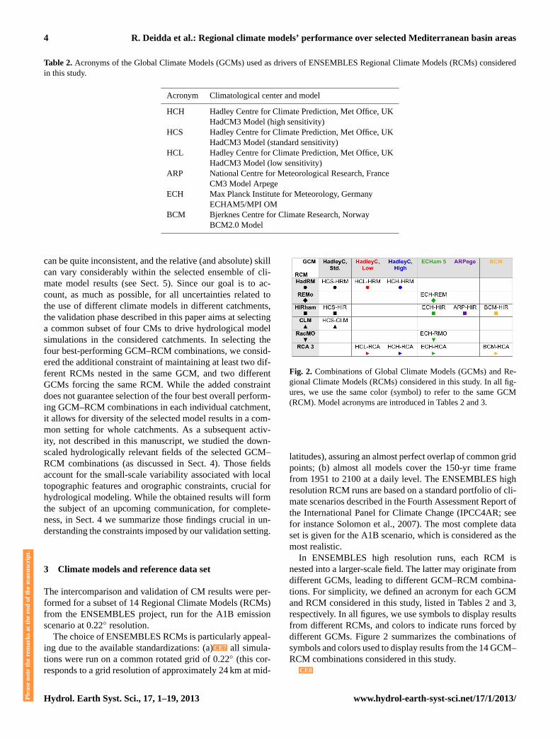
Fig. 2. Combinations of Global Climate Models (GCMs) and Re-gional Climate Models (RCMs) considered in this study. In all fig-ures, we use the same color (symbol) to refer to the same GCM(RCM). Model acronyms are introduced in Tables2 and3.

latitudes), assuring an almost perfect overlap of common gridpoints; (b) almost all models cover the 150-yr time framefrom 1951 to 2100 at a daily level. The ENSEMBLES highresolution RCM runs are based on a standard portfolio of cli-mate scenarios described in the Fourth Assessment Report ofthe International Panel for Climate Change (IPCC4AR; seefor instanceSolomon et al., 2007). The most complete dataset is given for the A1B scenario, which is considered as themost realistic.

In ENSEMBLES high resolution runs, each RCM isnested into a larger-scale field. The latter may originate fromdifferent GCMs, leading to different GCM–RCM combina-tions. For simplicity, we defined an acronym for each GCMand RCM considered in this study, listed in Tables2 and3,respectively. In all figures, we use symbols to display resultsfrom different RCMs, and colors to indicate runs forced bydifferent GCMs. Figure2 summarizes the combinations ofsymbols and colors used to display results from the 14 GCM–RCM combinations considered in this study.

CE8

Ple

ase

note

the

rem

arks

atth

een

dof

the

man

uscr

ipt.



Table 3.Acronyms of the Regional Climate Models (RCMs) considered in this study.

Acronym Climatological center and model

RCA Swedish Meteorological and Hydrological Institute (SMHI), SwedenRCA Model

HIR Danish Meteorological Institute (DMI), DenmarkHIRHAM5 Model

CLM Federal Institute of Technology of Zurich (ETHZ), SwitzerlandCLM Model

HRM Hadley Centre for Climate Prediction, Met Office, UKHadRM3Q3 Model

RMO Royal Netherlands Meteorological Institute (KNMI), NetherlandsRACMO2 Model

REM Max Planck Institute for Meteorology, Hamburg, GermanyREMO Model

Following the PCMDI/CMIP3 initiative, the ENSEM-BLES project stimulated and guided several climatic cen-ters towards standardization of model grids and outputs and,thus, promoted synergies across different research areas andinterdisciplinary efforts. Nevertheless, when pre-processingthe ENSEMBLES RCM outputs (i.e. before the validationphase), we experienced some minor discrepancies, requiringad hoc treatments. Although all issues were manageable, theyare worth mentioning, especially for scientists who are (orforesee) using these outputs to run hydrological models andperform impact studies:

– For most GCM–RCM combinations, the available timeframes cover the period from 1 January 1951 to 31 De-cember 2100. However, some model outputs exhibitmissing data on the last days of 2100, whereas forother models the missing values start at the end of2099. In addition, two model simulations (i.e. BCM–HIR, HCS–HIR) stop in year 2050, while the BCM–RCA model run starts in 1961.

– Models HCH–RCA, HCS–CLM, HCS–HRM, HCL–HRM, HCH–HRM, HCS–HIR, and HCL–RCA usea simplified calendar with 12 months of 30 days each(i.e. 360 days per year), whereas the remainder use astandard Gregorian calendar with 365 days per regularyear, and 366 days in leap years. Additionally, some ofthe last models mentioned do not account for the leapyear exception in 2100. We also detected some missingor incomplete data. More precisely, in some modelsthe values for the last days of the simulation period aresimply set to zero, rather than to an unambiguous de-fault flag for missing values. While this is not an issuewhen working with temperature fields expressed in K,it may create problems when considering precipitationfields (expressed in kg m−2 s−1), since it is not appar-ent how to distinguish between missing data and zeroprecipitation (this is the case, e.g. for the last 390 daysof data in the HCL–RCA simulation).

– For some models (see below), dry conditions areindicated by a very small positive or negative constantvalue,Pmin, whereas the sea level elevation is set toa constant value,zsea, different from zero. More pre-cisely, zsea≈ 0.046 m for HCH–RCA;zsea≈ 0.300 mfor BCM–HIR and HCS–HIR;zsea≈ 0.732 m andPmin ≈ −9.0× 10−8 kg m−2 s−1 for ECH–RMO;zsea≈ −0.002 m andPmin ≈ 1.7× 10−18 kg m−2 s−1

for ARP–HIR and ECH–HIR;zsea≈ −0.321 m andPmin ≈ −1.5× 10−11 kg m−2 s−1 for BCM–RCA,ECH–RCA and HCL–RCA. Also, for the last threemodels, missing temperature data at the end of thesimulation period are indicated by a minimum temper-ature of 0 K, whereas HCL–HRM simulations exhibitsome temperature values on the order of 1025 K. Whilethe origin of the aforementioned discrepancies in thedata cannot be easily identified (e.g. numerical errors,spurious effects of model parameterizations, routinesused to create the netCDF files in the ENSEMBLESarchive, etc.), one should properly treat them beforeusing CM outputs to perform climate change impactstudies. For example, unless properly identified, aminimum precipitation threshold may bias rainfallstatistics (e.g. the annual fraction of dry periods) and,from a practical point of view, influence hydrologicaland meteorological analysis (e.g. drought analysis).

For each considered catchment, the selected set of climatemodel data was validated using the E-OBS data set fromthe ENSEMBLES EU-FP6 project, made available by theECA&D project (http://www.ecad.eu) and hosted by the Cli-mate Research Unit (CRU) of the Hadley Centre. E-OBS datafiles are gridded observational data sets of daily precipitationand temperature, developed on the basis of a European net-work of high-quality historical measurements. In particular,we used version 5.0 of the E-OBS data set that covers the pe-riod from 1 January 1950 to 30 June 2011, and is available atfour different grid resolutions: 0.25 and 0.5◦ regular latitude–


http://www.ecad.eu


longitude grids, and 0.22 and 0.44◦ rotated pole grids. In ouranalysis, we use the rotated grid at 0.22◦ resolution, whichmatches the grid of ENSEMBLES RCMs exactly. Having analmost perfect point-to-point correspondence between EN-SEMBLES RCM results and E-OBS reference data, greatlysimplifies intercomparison, validation and calibration activ-ities, since no interpolation or re-gridding of the data isneeded. Results from any validation activity can be sensi-tive to the choice of the observational reference. It is alsoworth mentioning that in each of the considered countrieswhere CLIMB catchments are located, there are additionalstations not considered for E-OBS. However, access to anduse of their data is often problematic, due to administrativelimitations of the local competent authorities in distributingthe data, long inactivity periods of the stations, measuringerrors, missing values etc. Thus, in a multi-faceted projectlike CLIMB, E-OBS allows researchers to overcome techni-cal limitations, providing regular gridded data of the samequality and standards for all areas of interest.

There are several additional reasons why the E-OBS dataset is considered to be the best available source for tempera-ture and precipitation estimates in the considered catchmentsto pursue model validation: (1) E-OBS data have been ob-tained through kriging interpolation, which belongs to theclass of best linear unbiased estimators (BLUE); (2) the orig-inal data (i.e. prior to interpolation) have been properly cor-rected to minimize biases introduced by local effects andorography; (3) the 95 % confidence intervals of the obtainedestimates are also distributed, shedding light on the accuracyof the calculated areal averages, and (4) the surface-elevationfields used for E-OBS interpolations are available as well.The latter can be used to assess which counterpart of the ob-served differences between ENSEMBLES RCM and E-OBSclimatologies can be attributed to different orographic repre-sentations and, also, to remove biases introduced by eleva-tion differences in the E-OBS and corresponding RCM gridpoints. For example, to account for different surface eleva-tion models used by ENSEMBLES RCMs and E-OBS, andbefore calculating CM performance metrics, we used the cor-responding model orographies and a monthly constant lapserate to translate surface temperatures at different elevationsto those observed at sea level, as discussed in Sect. 4 below.For a more detailed description of the E-OBS data set, thereader is referred toHaylock et al.(2008).

4 Metrics for validation

Several studies (see Introduction) have focused on metrics toassess the accuracy of climate model results. Note, however,that performance metrics should depend on the specific useof climate data. In this study, we focus on providing reliableclimatic forcing for hydrological applications at a river-basinlevel. For this purpose, one needs to downscale the CM fieldsto resolutions suitable to run hydrological models and assess

climate change impacts. In the following, we summarize themain aspects of the downscaling procedure in order to makeour validation setting clearer. A detailed description of thedownscaling procedures, together with the obtained results,will form the subjects of an upcoming work.

Precipitation downscaling was performed using the mul-tifractal approach described inDeidda (2000) and Badaset al. (2006), starting from areal averages of daily precip-itation. The latter were obtained by averaging rainfall val-ues over a 4× 4 stencil of ENSEMBLES grid points cen-tered on each catchment, covering an approximate area of100 km× 100 km. This particular choice allowed for the em-bedding of all catchments inside equally sized spatial do-mains. The size of the latter is within the range of the space–time scale invariance of rainfall indicated by several studies(Schertzer and Lovejoy, 1987; Tessier et al., 1993; Perica andFoufoula-Georgiou, 1996; Venugopal et al., 1999; Deidda,2000; Kundu and Bell, 2003; Gebremichael and Krajewski,2004; Deidda et al., 2004, 2006; Gebremichael et al., 2006;Badas et al., 2006; Veneziano et al., 2006; Veneziano andLangousis, 2005, 2010) and, thus it can be used to define theintegral volume of rainfall to be downscaled to higher reso-lutions of a few square kilometers. That said, the validationmetrics of ENSEMBLES RCM simulations versus E-OBSdata are calculated based on areal rainfall averages over aregular 4× 4 grid-point stencil.

Temperature fields from ENSEMBLES RCMs weredownscaled based on the procedure described inListon andElder(2006), which combines a spatial interpolation scheme(Barnes, 1964, 1973) with orographic corrections. Although,in the case of temperature, downscaling starts from the EN-SEMBLES resolution (24 km× 24 km), we decided to adoptthe same validation setting as that for precipitation (i.e. calcu-lated areal averages of daily temperatures over a regular 4× 4grid-point stencil). Since temperature fields are particularlysensitive to elevation, in order to make homogeneous com-parisons, we first reduced surface temperatures at differentelevations to sea level, and then calculated areal averages ofdaily temperatures over a regular 4× 4 grid-point stencil cen-tered on each catchment. For the former, we used a standardmonthly lapse rate for the Northern Hemisphere (Kunkel,1989) and the corresponding ENSEMBLES model and E-OBS orographies. This appears to be a reasonable choicesince, after reduction to sea level, the temperature field be-comes quite smooth.

In summary, all metrics defined below are used to validateENSEMBLES RCM simulations vs. E-OBS data, using spa-tial averages of temperature and precipitation over a 4× 4grid-point stencil. This choice allows one to better study cli-matic forcing at a common catchment scale. An additionaladvantage is that spatial averaging smooths and filters outsome local biases present in E-OBS fields. These originatefrom the low density of observations, which prevents the ef-ficient capture of orographic effects on precipitation and tem-



perature and, also prevent the high spatial variability of dailyrainfall from being accounted for.

It is worth mentioning that the E-OBS data set is based onobservations obtained from a network of land-based stations.Hence, all E-OBS data over sea were masked and set to de-fault missing values. Nevertheless, missing values were alsofound at some grid points over land where the network den-sity is low. An analysis of the data density over time showedthat there are E-OBS grid points over land where the avail-ability of interpolated data depends on the period studied.This is due to changes in the observation network between1950 and 2011. To account for this issue, when calculatingareal averages of daily values over the 4× 4 grid-point sten-cil, we maintained those points with less than 6 yr of missingdata (i.e. 10 % of the 60 yr validation period from 1951 to2010). To that extent, all validation metrics below were cal-culated using those grid points available for both E-OBS dataand ENSEMBLES RCM simulations.

Following the discussion above, let us defineXm(s, y)

as the monthly spatial average of variableX (i.e. X =T ,P for monthly temperatures and rainfall intensities, respec-tively) over an area of approximately 100× 100 km (i.e. a4× 4 stencil of ENSEMBLES climate model outputs), pro-duced by climate modelm (m = 1, . . . , 14) for months

(s = 1, . . . , 12) in yeary (y = 1951, 1952, . . . , 2100). Accord-ing to this notation, let us also denote the index for E-OBSby m = 0. Thes-th monthly mean and standard deviation ofXm(s, y) over aNy yr climatological period starting in yeary0 are given by

µXm(s) =

1

Ny

y0+Ny−1∑y=y0

Xm(s, y), (1)

σXm (s) =

√√√√ 1

Ny − 1

y0+Ny−1∑y=y0

[Xm(s, y) − µX

m(s)]2

. (2)

The time window for validation is set to 60 yr (from 1951to 2010), entirely covered by E-OBS data. Validation of cli-mate model outputs over that period requires comparing spe-cific statistics ofXm (m = 1, . . . , 14) to those of E-OBS(i.e. Xm=0). To do so we introduce average error measuresfor the absolute differences between statistics of the observed(m = 0) and modeled (m = 1, . . . , 14) time series. Settingy0 = 1951 andNy = 60 in Eqs. (1) and (2), such error mea-sures for the monthly climatological means and standard de-viations ofXm, over the 60 yr period 1951–2010 are definedas

EµXm =

1

12

12∑s=1

∣∣∣µXm(s) − µX

0 (s)

∣∣∣ , (3)

EσXm =

1

12

12∑s=1

∣∣∣σXm (s) − σX

0 (s)

∣∣∣ . (4)

In addition, errors in the marginal distribution ofXm canbe quantified by averaging the absolute differences betweenthe quantilesxm(αi) of the observed (m = 0) and simu-lated (m = 1, . . . , 14) series at different probability levelsαi

(i = 1, . . . ,n):

EqXm =

1

n

n∑i=1

|xm (αi) − x0 (αi)| . (5)

The above-defined error metrics provide information on thereliability of a single variable, whereas for subsequent hy-drological modeling we need to identify those models thatperform best for a specific set of variables. As a minimum re-quirement for hydrological modeling, we seek for CMs thatprovide reliable estimates of precipitation and temperature:precipitation is the main source of water in the catchment,whereas temperature controls evaporation and evapotranspi-ration processes. Thus, in order to compare the performancesof different modelsm (m = 1, . . . , 14) in reproducing, si-multaneously, the statistics of the observed precipitation andtemperature fields, we introduce the following dimensionlessmeasures:

εµm = wP EµPm

M∑k=1

EµPk

+ wT EµTm

M∑k=1

EµTk

, (6)

ε σm = wP EσPm∑M

k=1 EσPk

+ wT Eσ Tm∑M

k=1 Eσ Tk

, (7)

whereM = 14 is the number of models, andwP andwT areweighting factors for precipitation and temperature errors, re-spectively, that satisfywP

+ wT = 1.Equations (6) and (7) can be used to assess the relative

performance of different models in reproducing the monthlymean and standard deviation of the observed temperature andprecipitation series. The weighting schemewP =wT = 0.5corresponds to the most neutral option (i.e. same weightsfor both precipitation and temperature). In the limiting casewhenwP = 1 andwT = 0, Eqs. (6) and (7) provide the sameinformation as Eqs. (3) and (4) when applied to precipita-tion, with the only difference being that the former equationslead to dimensionless error metrics. A similar setting holdsfor wP = 0 andwT = 1, where Eqs. (3) and (4) lead to dimen-sionless error metrics for temperature.

It is worth mentioning that proper weighting of precipi-tation and temperature errors in Eqs. (6) and (7) should inprinciple be determined by taking into account the structureand parameterization of the hydrological model used and itssensitivity to different forcing variables, as well as the cli-matology of the basin. However, within the CLIMB projecta variety of hydrological models have been applied (includ-ing fully distributed hydrological models as well as semi-distributed models), to a number of catchments with differentclimatologies. Under this setting, it was essential to conduct



a sensitivity analysis to different weighting schemes as de-scribed in Sect. 5.2.

5 Results and discussion

5.1 Seasonal distribution of precipitation andtemperature

When assessing models’ skills, it is important to exam-ine their ability to reproduce the annual averages and sea-sonal variability of precipitation and surface temperature.These two variables specify the climate type according to theKöppen–Geiger climate classification system. Thus, a firstskill measure is the ability of the models to reproduce thelocal climatic characteristics of specific basins.

Figures 3 and 4 show the mean monthly precipitation andtemperature for each catchment, calculated using Eq. (1),for the Ny = 60 yr verification period (1951–2010). For theE-OBS observational reference, we use a dotted black line,whereas ENSEMBLES RCM results are plotted using thereference introduced in Fig. 2. Based on the E-OBS seasonalvariation of precipitation and temperature, Thau, Riu Mannu,Kokaeli and Chiba are characterized by a Mediterranean cli-mate, with precipitation maxima in winter, and minima insummer. Gaza, although exhibiting a seasonal cycle of pre-cipitation similar to the previously mentioned basins, is clas-sified as semi-arid due to its low annual precipitation andhigh mean annual temperature. Noce, by contrast, has a hu-mid continental climate, receiving regular precipitation dur-ing the year, with a single maximum during summer. Inessence, although based on a sparse network, E-OBS datareproduce quite reasonably the expected seasonal climato-logical patterns in the considered catchments.

In comparing model results for precipitation with E-OBSobservational data, Fig. 3 clearly shows significant discrep-ancies between ENSEMBLES RCMs and E-OBS climatolo-gies, both in terms of magnitude and, in some cases, theobserved seasonal cycle. In almost all catchments, severalRCMs produce higher annual precipitation than that ob-served. In more detail: for Thau, Riu Mannu and Noce, 11 outof 14 models simulate higher precipitation amounts for atleast ten months of the year. The same problem is detectedfor 9 RCMs in Kokaeli and 8 RCMs in Chiba catchments.An additional observation is that, in all catchments exceptGaza, RCMs exhibit a larger relative error for high precipita-tion amounts in summer months. This positive bias is ampli-fied in catchments with Mediterranean climate, where RCMprecipitation can be up to ten times higher than the observedprecipitation. In Gaza, on the other hand, models are typi-cally biased towards lower values of precipitation, with theexception of a handful of models, which are instead biasedtowards larger precipitation amounts. Note, also, that onemodel, BCM–RCA, produces unrealistic results.

A catchment where models’ skills are problematic isRiu Mannu: while E-OBS indicates almost no precipitationduring the summer months of June–August, some models(HCL–RCA, BCM–HIR, BCM–RCA, HCH–HRM) displayrelatively high amounts of summer precipitation. Althoughthe skill of RCMs in reproducing seasonal precipitation isgenerally weaker during summer, especially for the driersouthern and eastern European regions (Frei et al., 2006; Ma-raun et al., 2010), this finding is still surprising, since severalstudies indicate that RCMs tend to underestimate precipita-tion during summer (e.g.Jacob et al., 2007).

Figure 3 also shows that, despite the aforementioned bi-ases, almost all models predict a reliable seasonal precipita-tion cycle for the Thau, Riu Mannu, Kocaeli, Chiba and Gazacatchments. By contrast, RCMs fail to capture the seasonalcycle of precipitation in the Noce catchment: instead of asingle maximum during summer, most models display a bi-modal behavior, with one maximum before the summer sea-son and one directly following it. This pattern indicates a hu-mid subtropical climate, typical of most lowlands in AdriaticItaly, south of the Noce region. A possible reason is that, at24 km resolution, RCMs are limited in resolving small-scalefeatures necessary to correctly reproduce orographic precip-itation. Moreover, the observed differences between CM re-sults and E-OBS observational data might stem from the ir-regular and sparse network of E-OBS stations, especially inview of the fact that most stations are located at low altitudes.

Unsurprisingly, RCMs tend to perform better in modelingsurface temperature. Figure 4 shows that all RCMs reproducea reliable yearly cycle of monthly climatological tempera-tures (previously reduced to sea level, see Sect. 4). Neverthe-less, when compared to E-OBS, several RCMs exhibit sig-nificant biases (often larger than 5 K), while the inter-modelspread can be as large as 10 K (especially during summer).In more detail: for Noce, HCL–RCA exhibits a negative biaslarger than 5 K during winter; for Kocaeli, ECH–HIR ex-hibits a positive bias of about 4 K during winter; whereas forChiba, HCL–HRM overestimates temperature during sum-mer by 5 K. However, given the good representation of theseasonal temperature cycle, these discrepancies can be prop-erly reduced using simple bias-correction techniques.

5.2 Selection of best-performing ENSEMBLES models

Error metrics introduced in Eqs. (3) and (4) were calculatedfor each ENSEMBLES RCM for the 60 yr verification periodfrom 1951 to 2011CE9, and then plotted for each catchmentin a separate scatter plot (Fig. 5). One sees that, in all catch-ments except Noce, most models (i.e. 11 out of 14 modelsof the Thau basin; 13 models of the Riu Mannu and Kocaelicatchments, and all 14 models of Gaza and Chiba) exhibiterrors lower than 1.5 mm d−1 in their monthly means,EµP,and lower than 1 mm d−1 in their monthly standard devia-tions,EσP. For Noce basin, the corresponding errors are sig-nificantly larger.

Ple

ase

note

the

rem

arks

atth

een

dof

the

man

uscr

ipt.



Jan Feb Mar Apr May Jun Jul Aug Sep Oct Nov Dec0

50

100

150

200

250

Mon

thly

Pre

cipi

tatio

n M

ean

µP [m

m]

Catchment "thau" − Validation period: 1951−2010

HCS−HRMHCS−HIRHCS−CLMHCL−HRMHCL−RCAHCH−HRMHCH−RCAECH−REMECH−HIRECH−RMOECH−RCAARP−HIRBCM−HIRBCM−RCAE−OBS


20

40

60

80

100

120

140

Mon

thly

Pre

cipi

tatio

n M

ean

µP [m

m]

Catchment "riumannu" − Validation period: 1951−2010



50

100

150

200

250

300

350

400

Mon

thly

Pre

cipi

tatio

n M

ean

µP [m

m]

Catchment "noce" − Validation period: 1951−2010



20

40

60

80

100

120

140

160

180

Mon

thly

Pre

cipi

tatio

n M

ean

µP [m

m]

Catchment "kokaeli" − Validation period: 1951−2010



50

100

150

200

250

300

Mon

thly

Pre

cipi

tatio

n M

ean

µP [m

m]

Catchment "gaza" − Validation period: 1951−2010



10

20

30

40

50

60

70

80

90

Mon

thly

Pre

cipi

tatio

n M

ean

µP [m

m]

Catchment "chiba" − Validation period: 1951−2010


Fig. 3. Mean monthly precipitation (mm) over the 60 yr verification period (1951–2100) for the 14 ENSEM-BLES models and E-OBS. Each subplot displays areal averages over a 4×4 grid-point stencil centered in eachcatchment.

22

Fig. 3. Mean monthly precipitation (mm) over the 60 yr verification period (1951–2100) for the 14 ENSEMBLES models and E-OBS. Eachsubplot displays areal averages over a 4× 4 grid-point stencil centered on each catchment.

Concerning the temperature error metrics,EµT andEσ T ,in Fig. 6, one notes that the error in the monthly means ismuch larger than the one in the standard deviations: for al-most all models and most catchments (i.e. all models of theThau, Riu Mannu and Chiba basins, 13 out of 14 modelsof the Kocaeli catchment, and 12 out of 14 models of Noceand Gaza),EµT andEσ T are smaller than 3 and 0.5 K, re-spectively. Again, one concludes that Noce is the catchmentwhere ENSEMBLES RCMs tend to perform even worse fortemperature: only 4 out of 14 models exhibit errors smallerthan 1.5 K inEµT . Note that in Gaza (the second-worst per-

forming catchment), 8 out of 14 RCMs exhibit errors smallerthan 1.5 K inEµT . Concerning Noce basin, it is worth not-ing that one cannot easily conclude to what extent the cal-culated temperature and precipitation errors originate fromlimitations of the observational network at high elevations inthe Alps.

Figures 5 and 6 also show that model performances canvary significantly from one catchment to another. For in-stance, HCS–CLM is one of the two worst performers re-garding modeling precipitation in Thau, but it performs bestregarding modeling precipitation in Noce (see Fig. 5). For




280

285

290

295

300

305

Mon

thly

Tem

pera

ture

Mea

n (a

t sea

leve

l) µT

[K]




285

290

295

300

305

310

Mon

thly

Tem

pera

ture

Mea

n (a

t sea

leve

l) µT

[K]




275

280

285

290

295

300

305

Mon

thly

Tem

pera

ture

Mea

n (a

t sea

leve

l) µT

[K]




280

285

290

295

300

305

Mon

thly

Tem

pera

ture

Mea

n (a

t sea

leve

l) µT

[K]




285

290

295

300

305

Mon

thly

Tem

pera

ture

Mea

n (a

t sea

leve

l) µT

[K]




285

290

295

300

305

Mon

thly

Tem

pera

ture

Mea

n (a

t sea

leve

l) µT

[K]



Fig. 4. Same as Fig. 3, but for mean monthly temperatures (K) reduced to sea level.

23

Fig. 4.Same as Fig.3, but for mean monthly temperatures (K) reduced to sea level.

all models, precipitation errors in Gaza are quite small (seeFig. 5), while temperature errors are significant (see Fig. 6).This means that, as expected, of all of the considered RCMs,it is not possible to identify a subset of models that performsbest for both variables in all catchments. One option is tobase model selection on dimensionless metrics capable ofweighting the errors in the variables of interest, even whenthe choice is driven by additional constraints as discussedin Sect. 2. With this aim, we introduced the dimensionlesserror metrics in Eqs. (6) and (7) to account for both precip-itation and temperature RCM performances in reproducingE-OBS observational data. As discussed in Sect. 4, proper

selection of precipitation- and temperature-weighting factors(wP ,wT ) in Eqs. (6) and (7) should account for the structureand parameterization of the hydrological model used and itssensitivity to different forcing variables, as well as the clima-tology of the basin. Given the variety of catchments and hy-drological models considered in the CLIMB project, we per-formed a sensitivity analysis to different (wP, wT ) weightingschemes, covering the whole range of (wP = 1,wT = 0; high-est precipitation weighting) to (wP = 0, wT = 1; highest tem-perature weighting). As an example, Fig. 7 shows results forthe neutral case, i.e. equal weights for precipitation and tem-perature errors (i.e.wP = 0.5,wT = 0.5). One sees that the se-



0 0.5 1 1.5 2 2.5 3 3.5 40

0.5

1

1.5

2

2.5

3

3.5

4

EµP [mm/d]

EσP

[mm

/d]


HCS−HRMHCS−HIRHCS−CLMHCL−HRMHCL−RCAHCH−HRMHCH−RCAECH−REMECH−HIRECH−RMOECH−RCAARP−HIRBCM−HIRBCM−RCA

0 0.5 1 1.5 2 2.5 3 3.5 40

0.5

1

1.5

2

2.5

3

3.5

4

EµP [mm/d]

EσP

[mm

/d]



0 0.5 1 1.5 2 2.5 3 3.5 40

0.5

1

1.5

2

2.5

3

3.5

4

EµP [mm/d]

EσP

[mm

/d]



0 0.5 1 1.5 2 2.5 3 3.5 40

0.5

1

1.5

2

2.5

3

3.5

4

EµP [mm/d]

EσP

[mm

/d]



0 0.5 1 1.5 2 2.5 3 3.5 40

0.5

1

1.5

2

2.5

3

3.5

4

EµP [mm/d]

EσP

[mm

/d]



0 0.5 1 1.5 2 2.5 3 3.5 40

0.5

1

1.5

2

2.5

3

3.5

4

EµP [mm/d]

EσP

[mm

/d]



Fig. 5. Scatterplot of errors in the mean and standard deviation of monthly precipitation (mm d−1) over the60 yr verification period (1951–2100), computed using Eqs. (3) and (4) for each of the 14 ENSEMBLES modelswith respect to E-OBS observational reference. Each subplot displays areal averages over a 4× 4 grid-pointstencil centered in each catchment. 24

Fig. 5.Scatter plot of errors in the mean and standard deviation of monthly precipitation (mm d−1) over the 60 yr verification period (1951–2010), computed using Eqs. (3) and (4) for each of the 14 ENSEMBLES models with respect to E-OBS observational reference. Each subplotdisplays areal averages over a 4× 4 grid-point stencil centered in each catchment.

lection of HCH–RCA, ECH–RCA, ECH–RMO, ECH–REMmodels (marked with an additional black circle) are the bestchoices for the Thau, Riumannu, Kokaeli and Chiba catch-ments, under the additional constraint of maintaining twodifferent RCMs nested in the same GCM, and two differentGCMs forcing the same RCM. For Noce and Gaza, for whichother choices would have been slightly better, the selectedfour models still display good performances. Although not

presented here, similar results were obtained for all possiblecouples of weights, making us confident that our selectionof the four best-performing models is robust, regardless ofthe hydrological model framework. Concerning the limitingcases (wP = 1,wT = 0) and (wP = 0,wT = 1), Eqs. (6) and (7)correspond to dimensionless variants of Eqs. (3) and (4), re-spectively. Thus, Figs. 5 and 6 allow one to conclude that thefour best-performing models identified using equal precipita-



0 0.5 1 1.5 2 2.5 3 3.5 40

0.5

1

1.5

2

2.5

3

3.5

4

EµT [K]

EσT

[K]



0 0.5 1 1.5 2 2.5 3 3.5 40

0.5

1

1.5

2

2.5

3

3.5

4

EµT [K]

EσT

[K]



0 0.5 1 1.5 2 2.5 3 3.5 40

0.5

1

1.5

2

2.5

3

3.5

4

EµT [K]

EσT

[K]



0 0.5 1 1.5 2 2.5 3 3.5 40

0.5

1

1.5

2

2.5

3

3.5

4

EµT [K]

EσT

[K]



0 0.5 1 1.5 2 2.5 3 3.5 40

0.5

1

1.5

2

2.5

3

3.5

4

EµT [K]

EσT

[K]



0 0.5 1 1.5 2 2.5 3 3.5 40

0.5

1

1.5

2

2.5

3

3.5

4

EµT [K]

EσT

[K]



Fig. 6. Same as Fig. 5, but for temperatures (K) reduced to sea level.

25

Fig. 6.Same as Fig.5, but for temperatures (K) reduced to sea level.

tion and temperature weights, remain best also in the limitingcases of highest precipitation (wP = 1,wT = 0) or temperature(wP = 0,wT = 1) weightings.

In order to check the general behavior of the probabilitydistributions of the simulated precipitation and temperaturefields against E-OBS, we used Eq. (5) to compute the meanabsolute errors in the quantiles at 100 uniformly spaced prob-ability levels. The results are presented in the scatter plots ofFig. 8. One sees that the 4 selected models display reasonableperformances in all considered catchments, thus confirming

the selection. To assist the reader in identifying the 4 selectedmodels in all figures, we have drawn thicker the correspond-ing lines in Figs. 3 and 4, and added black circles in all scatterplots (Figs. 5–8).

Last but not least, it is interesting to analyze and inter-compare the variability of the mean annual precipitation andtemperature over the five 30 yr climatological periods be-tween 1951 and 2100. In Fig. 9, where results for precipi-tation are presented, one clearly observes a very large vari-ability in the simulations of the 14 models, with some models

Ple

ase

note

the

rem

arks

atth

een

dof

the

man

uscr

ipt.



0 0.02 0.04 0.06 0.08 0.1 0.12 0.14 0.16 0.18 0.20

0.02

0.04

0.06

0.08

0.1

0.12

0.14

0.16

0.18

0.2

ε µ [−]

ε σ

[−]



0 0.02 0.04 0.06 0.08 0.1 0.12 0.14 0.16 0.18 0.20

0.02

0.04

0.06

0.08

0.1

0.12

0.14

0.16

0.18

0.2

ε µ [−]

ε σ

[−]



0 0.02 0.04 0.06 0.08 0.1 0.12 0.14 0.16 0.18 0.20

0.02

0.04

0.06

0.08

0.1

0.12

0.14

0.16

0.18

0.2

ε µ [−]

ε σ

[−]



0 0.02 0.04 0.06 0.08 0.1 0.12 0.14 0.16 0.18 0.20

0.02

0.04

0.06

0.08

0.1

0.12

0.14

0.16

0.18

0.2

ε µ [−]

ε σ

[−]



0 0.02 0.04 0.06 0.08 0.1 0.12 0.14 0.16 0.18 0.20

0.02

0.04

0.06

0.08

0.1

0.12

0.14

0.16

0.18

0.2

ε µ [−]

ε σ

[−]



0 0.02 0.04 0.06 0.08 0.1 0.12 0.14 0.16 0.18 0.20

0.02

0.04

0.06

0.08

0.1

0.12

0.14

0.16

0.18

0.2

ε µ [−]

ε σ

[−]



Fig. 7. Same as Fig. 5, but for the dimensionless error metrics accounting for both precipitation and temperature,as defined in Eqs. (6) and (7).

26

Fig. 7.Same as Fig.5, but for the dimensionless error metrics accounting for both precipitation and temperature, as defined in Eqs. (6) and (7).

predicting mean annual precipitation three times higher thanothers. One also gets an idea of how drastically the behaviorof a single model can change for different catchments. Thesefindings support the need for extensive analyses, like the onepresented here, before proceeding with hydrological mod-eling in specific catchments. For example, the HECCE10–HIR model gives the largest annual precipitation in Thau andNoce, greatly overestimating E-OBS, while the same modelgives a very small annual precipitation for Riu Mannu andGaza, greatly underestimating E-OBS. The five 30 yr clima-tologies for the 4 selected models are shown in Fig. 9 inside

vertical rectangles. Again, one visually observes that the se-lection of the four models is a reasonable compromise for allcatchments.

An additional observation one makes is that, for eachcatchment, the variability in the 30 yr climatological peri-ods for a single model is much smaller than the variabil-ity among different models. Figure 10 shows similar resultsfor temperatures, where the variability among different mod-els, although still larger than the variability among the 30 yrclimatological periods for a single model, is of comparablemagnitude.



0 0.5 1 1.5 2 2.5 3 3.5 4 4.5 5 5.50

0.5

1

1.5

2

2.5

3

3.5

4

4.5

5

5.5

Quantile errors for Temperature [K]

Qua

ntile

err

ors

for

Pre

cipi

tatio

n [m

m/d

]



0 0.5 1 1.5 2 2.5 3 3.5 4 4.5 5 5.50

0.5

1

1.5

2

2.5

3

3.5

4

4.5

5

5.5


Qua

ntile

err

ors

for

Pre

cipi

tatio

n [m

m/d

]



0 0.5 1 1.5 2 2.5 3 3.5 4 4.5 5 5.50

0.5

1

1.5

2

2.5

3

3.5

4

4.5

5

5.5


Qua

ntile

err

ors

for

Pre

cipi

tatio

n [m

m/d

]



0 0.5 1 1.5 2 2.5 3 3.5 4 4.5 5 5.50

0.5

1

1.5

2

2.5

3

3.5

4

4.5

5

5.5


Qua

ntile

err

ors

for

Pre

cipi

tatio

n [m

m/d

]



0 0.5 1 1.5 2 2.5 3 3.5 4 4.5 5 5.50

0.5

1

1.5

2

2.5

3

3.5

4

4.5

5

5.5


Qua

ntile

err

ors

for

Pre

cipi

tatio

n [m

m/d

]



0 0.5 1 1.5 2 2.5 3 3.5 4 4.5 5 5.50

0.5

1

1.5

2

2.5

3

3.5

4

4.5

5

5.5


Qua

ntile

err

ors

for

Pre

cipi

tatio

n [m

m/d

]



Fig. 8. Scatterplots of mean absolute errors in the quantiles of daily precipitation and temperature distributions,computed using Eq. (8) for each of the 14 ENSEMBLES models with respect to E-OBS observational reference.Quantiles are calculated at 100 uniformly spaced probability levels. Each subplot displays areal averages overa 4× 4 grid-point stencil centered in each catchment. 27

Fig. 8. Scatter plots of mean absolute errors in the quantiles of daily precipitation and temperature distributions, computed using Eq. (8)for each of the 14 ENSEMBLES models with respect to E-OBS observational reference. Quantiles are calculated at 100 uniformly spacedprobability levels. Each subplot displays areal averages over a 4× 4 grid-point stencil centered in each catchment.

6 Conclusions

Validation of climate models is typically performed using ob-servational data, by studying the skills of different models inreproducing climate features in the study area. One majortask is the choice of such observations. This study focuseson providing reliable climatic forcing for hydrological ap-plications at a river-basin level and, therefore precipitation

and surface temperature were chosen as verification variablessince (a) they are used to specify the climate of a regionin several climate classification systems, like the Köppen–Geiger one, (b) they represent a minimum requirement forhydrological modeling, being, respectively, the main sourceof water in the catchments and the main control parameterfor evaporation and evapotranspiration, and (c) precipitation-and temperature- observation networks are the most dense



0 2 4 6 8 10 12 14 16 18 20400

500

600

700

800

900

1000

1100

1200

1300

30−

y P

reci

pita

tion

mea

n [m

m/y

]

Catchment "thau" − Interperiod variability (1951−2100)

1 − HCS−HRM2 − HCS−HIR3 − HCS−CLM4 − HCL−HRM5 − HCL−RCA6 − HCH−HRM7 − HCH−RCA8 − ECH−REM9 − ECH−HIR10 − ECH−RMO11 − ECH−RCA12 − ARP−HIR13 − BCM−HIR14 − BCM−RCA15 − E−OBS

0 2 4 6 8 10 12 14 16 18 20200

300

400

500

600

700

800

900

1000

1100

30−

y P

reci

pita

tion

mea

n [m

m/y

]

Catchment "riumannu" − Interperiod variability (1951−2100)


0 2 4 6 8 10 12 14 16 18 20800

1000

1200

1400

1600

1800

2000

2200

2400

2600

2800

30−

y P

reci

pita

tion

mea

n [m

m/y

]

Catchment "noce" − Interperiod variability (1951−2100)


0 2 4 6 8 10 12 14 16 18 20300

400

500

600

700

800

900

1000

1100

1200

30−

y P

reci

pita

tion

mea

n [m

m/y

]

Catchment "kokaeli" − Interperiod variability (1951−2100)


0 2 4 6 8 10 12 14 16 18 200

500

1000

1500

30−

y P

reci

pita

tion

mea

n [m

m/y

]

Catchment "gaza" − Interperiod variability (1951−2100)


0 2 4 6 8 10 12 14 16 18 20100

150

200

250

300

350

400

450

500

550

600

30−

y P

reci

pita

tion

mea

n [m

m/y

]

Catchment "chiba" − Interperiod variability (1951−2100)


Fig. 9. Variability of the mean annual precipitation (mm yr−1) over the five 30 yr climatological periods be-tween 1951 and 2100. Models HCS-HIR and BCM-HIR stop in year 2050. The reference values of E-OBSclimatologies in the two 30 yr periods between 1951–2010 are indicated with empty circles and horizontal lines.Each subplot displays results based on areal averages over a 4×4 grid-point stencil centered in each catchment.

28

Fig. 9. Variability of the mean annual precipitation (mm yr−1) over the five 30 yr climatological periods between 1951 and 2100. ModelsHCS–HIR and BCM–HIR stop in year 2050. The reference values of E-OBS climatologies in the two 30 yr periods between 1951–2010are indicated with empty circles and horizontal lines. Each subplot displays results based on areal averages over a 4× 4 grid-point stencilcentered on each catchment.

and readily available ones (in contrast to, say, radiation- orevapotranspiration-measurement networks).

Another basic problem of model validation is that of se-lecting appropriate metrics to weight the relative influenceof different variables. Since we needed to compare modelperformances in simultaneously reproducing the statistics oftemperature and precipitation fields, we introduced dimen-sionless normalized metrics.

RCMs have been used in two major scientific projects,PRUDENCE and ENSEMBLES, to produce future climateprojections for the European UnionCE11. The correspondingmodel simulations have been studied and validated in sev-eral recent papers (i.e. Christensen and Christensen, 2007,for PRUDENCE; and Lorenz and Jacob, 2010TS1, for EN-SEMBLES). While most validation studies examined modelperformances by focusing on medium- to large-scale areas(e.g. Christensen et al., 2010TS2, and Kjellström et al., 2010,

Ple

ase

note

the

rem

arks

atth

een

dof

the

man

uscr

ipt.



0 2 4 6 8 10 12 14 16 18 20284

286

288

290

292

294

296

30−

y T

empe

ratu

re m

ean

[K]

Catchment "thau" − Interperiod variability (1951−2100)


0 2 4 6 8 10 12 14 16 18 20288

289

290

291

292

293

294

295

296

297

298

30−

y T

empe

ratu

re m

ean

[K]

Catchment "riumannu" − Interperiod variability (1951−2100)


0 2 4 6 8 10 12 14 16 18 20282

284

286

288

290

292

294

296

30−

y T

empe

ratu

re m

ean

[K]

Catchment "noce" − Interperiod variability (1951−2100)


0 2 4 6 8 10 12 14 16 18 20286

287

288

289

290

291

292

293

294

295

30−

y T

empe

ratu

re m

ean

[K]

Catchment "kokaeli" − Interperiod variability (1951−2100)


0 2 4 6 8 10 12 14 16 18 20290

291

292

293

294

295

296

297

298

299

30−

y T

empe

ratu

re m

ean

[K]

Catchment "gaza" − Interperiod variability (1951−2100)


0 2 4 6 8 10 12 14 16 18 20289

290

291

292

293

294

295

296

297

298

299

30−

y T

empe

ratu

re m

ean

[K]

Catchment "chiba" − Interperiod variability (1951−2100)


Fig. 10. Same as Fig. 9, but for temperatures (K) reduced to sea level.

29

Fig. 10.Same as Fig.9, but for temperatures (K) reduced to sea level.

studied ENSEMBLES RCM results by dividing Europe intoseveral large areas), RCMs were found to only partially re-produce climate patterns in Europe (Jacob et al., 2007; Chris-tensen et al., 2010TS3).

Our study suggests that when interest is at relatively smallspatial scales associated with hydrological catchments, as itis the case of CLIMB project, validation of CM results shouldbe conducted at a single-basin level rather than at macro-regional scales. In this case, it is necessary to check models’skills in reproducing prescribed observations at specific riverbasins, since averaging over quite large areas might bias the

assessment. For example, for Riu Mannu, Thau and Chibacatchments, model performances can vary significantly (seeSect. 5), even though these catchments are included in thesame large-scale area in theChristensen and Christensen(2007) study.

In this work we validated RCM results at scales suitable torun hydrological models and conduct climate impact studiesfor representative Mediterranean catchments. We found thatthe performance of a single RCM in reproducing observa-tional data can change significantly for different river basins.This finding highlights the need for extensive analyses of



climate model outputs before proceeding with hydrologicalmodeling in specific catchments.

Another important finding is that, at least for temperatureand precipitation studied at a river-basin level, the variabil-ity in the 30 yr climatological periods for a single model ismuch smaller than the variability among different models, asFigs. 9 and 10 clearly show. We also stressed that the vali-dation process in complex terrains, such as the Alps (Nocecatchment), may be significantly affected by weaknesses ofmodel grids and the representativeness of the observationalnetwork. Actually, it can be problematic to interpret the dif-ferences between model outputs and observations, since theymay originate from a combination of issues: (a) the modelgrid is too coarse (e.g. the Noce case, located in the Alps,where the maximum elevation considered by the modelsis approximately 2500 m, quite lower than real orography);and (b) the observational network is too sparse to provide aproper basis for models’ validation.

Projects like ENSEMBLES and PRUDENCE stimulatedand guided several climatic centers towards standardiza-tion of procedures, model grids and outputs and, thus, pro-moted synergies across different research areas and interdis-ciplinary efforts. Nevertheless, our study indicates that er-rors and inconsistencies are still present, suggesting basin-specific pre-processing of CM outputs before proceedingwith hydrological modeling and climate impact assessments.

As to what concerns hydrological applications, we notethat while our validation-based model selection provides areasonable indication of the four best-performing modelsin the considered catchments, some model deficiencies stillneed to be addressed. Specifically, by applying bias- andquantile-correction techniques, we were able to reduce thedifferences between observed and modeled probability dis-tributions. In addition, by accounting for the effects of orog-raphy on precipitation, temperature and other variables, andmaking proper use of downscaling tools, we reproduced lo-cal climate attributes and, to some extent, the observed small-scale variability. These results, as well as hydrological mod-eling projections in the considered catchments (currently ad-dressed by several working groups of the CLIMB project)will form the subjects of forthcoming works.

Acknowledgements.This study has been developed within theproject CLIMB (Climate Induced Changes on the Hydrology ofMediterranean Basins: Reducing Uncertainty and QuantifyingRisk through an Integrated Monitoring and Modeling System,http://www.climb-fp7.eu), funded by the European Commission’s7th Framework Programme. We acknowledge the ENSEMBLESproject (http://ensembles-eu.metoffice.com), funded by the EU-FP6through contract GOCE-CT-2003-505539, and the data providersin the ECA&D project (http://www.ecad.eu) for making RCMsoutputs and the E-OBS data set available. CRS4 also acknowledgesthe contribution from Sardinian regional authorities.

Edited by: E. Morin

References

Annan, J. D., Hargreaves, J. C., and Tachiiri, K.: On the observa-tional assessment of climate model performance, Geophys. Res.Lett., 38, L24702, doi:10.1029/2011GL049812, 2011.

Badas, M. G., Deidda, R., and Piga, E.: Modulation of ho-mogeneous space-time rainfall cascades to account for oro-graphic influences, Nat. Hazards Earth Syst. Sci., 6, 427–437,doi:10.5194/nhess-6-427-2006, 2006.

Barnes, S. L.: A technique for maximazing details in numericalweather map analysis, J. Appl. Meteorol., 3, 396–409, 1964.

Barnes, S. L.: Mesoscale objective analysis using weighted time-setime observations, NOAA Tech. Memo. ERL NSSL-62,Tech. rep., National Severe Storms Laboratory, Norman, OK,1973.

Becker, A. and Grünewald, U.: Flood risk in Central Europe, Sci-ence, 300, 1099, doi:10.1126/science.1083624, 2003.

Cane, D., Barbarino, S., Renier, L. A., and Ronchi, C.: Regionalclimate models downscaling in the Alpine area with multi-model superensemble, Hydrol. Earth Syst. Sci., 17, 2017–2028,doi:10.5194/hess-17-2017-2013, 2013.

Christensen, J. H. and Christensen, O. B.: A summary of thePRUDENCE model projections of changes in European cli-mate by the end of this century, Climatic Change, 81, 7–30,doi:10.1007/s10584-006-9210-7, 2007.

Christensen, J. H., Machenhauer, B., Jones, R., Schär, C., Ruti, P.,Castro, M., and Visconti, G.: Validation of present-day re-gional climate simulations over Europe: LAM simulations withobserved boundary conditions, Clim. Dynam., 13, 489–506,doi:10.1007/s003820050178, 1997.

Deidda, R.: Rainfall downscaling in a space-time multifractalframework, Water Resour. Res., 36, 1779–1794, 2000.

Deidda, R., Badas, M. G., and Piga, E.: Space-time scaling in high-intensity Tropical Ocean Global Atmosphere Coupled Ocean-Atmosphere Response Experiment (TOGA-COARE) storms,Water Resour. Res., 40, W02506, doi:10.1029/2003WR002574,2004.

Deidda, R., Badas, M. G., and Piga, E.: Space-time multifractal-ity of remotely sensed rainfall fields, J. Hydrol., 322, 2–13,doi:10.1016/j.jhydrol.2005.02.036, 2006.

Fowler, H., Blenkinsop, S., and Tebaldi, C.: Linking climate changemodelling to impacts studies: recent advances in downscalingtechniques for hydrological modelling, Int. J. Climatol., 27,1547–1578, 2007.

Frei, C., Schöll, R., Fukutome, S., Schmidli, J., and Vidale, P. L.:Future change of precipitation extremes in Europe: Intercompar-ison of scenarios from regional climate models, J. Geophys. Res.,111, D06105, doi:10.1029/2005JD005965, 2006.

Gebremichael, M. and Krajewski, W.: Assessment of the statisti-cal characterization of small-scale rainfall variability from radar:analysis of TRMM ground validation datasets, J. Appl. Meteo-rol., 43, 1180–1199, 2004.

Gebremichael, M., Over, T., and Krajewski, W.: Comparison of thescaling characteristics of rainfall derived from space-based andground-based radar observations, J. Hydrometeorol., 7, 1277–1294, 2006.

Giorgi, F. and Mearns, L. O.: Introduction to special section: re-gional climate modeling revisited, J. Geophys. Res., 104, 6335–6352, doi:10.1029/98JD02072, 1999.




http://www.ecad.eu

http://dx.doi.org/10.1029/2011GL049812

http://dx.doi.org/10.5194/nhess-6-427-2006

http://dx.doi.org/10.1126/science.1083624

http://dx.doi.org/10.5194/hess-17-2017-2013

http://dx.doi.org/10.1007/s10584-006-9210-7

http://dx.doi.org/10.1007/s003820050178

http://dx.doi.org/10.1029/2003WR002574

http://dx.doi.org/10.1016/j.jhydrol.2005.02.036

http://dx.doi.org/10.1029/2005JD005965

http://dx.doi.org/10.1029/98JD02072


Giorgi, F. and Mearns, L.: Calculation of average, uncertainty range,and reliability of regional climate changes from AOGCM simu-lations via the Reliability Ensemble Averaging (REA) Method,J. Climate, 15, 1141–1158, 2002.

Gleckler, P. J., Taylor, K. E., and Doutriaux, C.: Performancemetrics for climate models, J. Geophys. Res., 113, D06104,doi:10.1029/2007JD008972, 2008.

Guyennon, N., Romano, E., Portoghese, I., Salerno, F., Calmanti,S., Petrangeli, A. B., Tartari, G., and Copetti, D.: Benefits fromusing combined dynamical-statistical downscaling approaches –lessons from a case study in the Mediterranean region, Hydrol.Earth Syst. Sci., 17, 705–720, doi:10.5194/hess-17-705-2013,2013.

Haylock, M. R., Hofstra, N., Klein-Tank, A. M. G., Klok, E. J.,Jones, P. D., and New, M.: A European daily high-resolution gridded data set of surface temperature and pre-cipitation for 1950–2006, J. Geophys. Res., 113, D20119,doi:10.1029/2008JD010201, 2008.

Jacob, D., Baerring, L., Christensen, O. B., Christensen, J. H.,de Castro, M., Deque, M., Giorgi, F., Hagemann, S., Hirschi, M.,Jones, R., Kjellstroem, E., Lenderink, G., Rockel, B.,Sanchez, E., Schaer, C., Seneviratne, S. I., Somot, S., vanUlden, A., and van den Hurk, B.: An inter-comparison of regionalclimate models for Europe: model performance in present-dayclimate, Climatic Change, 81, 31–52, doi:10.1007/s10584-006-9213-4, 2007.

Johnson, F. and Sharma, A.: Measurement of GCM Skill in Predict-ing Variables Relevant for Hydroclimatological Assessments, J.Climate, 22, 4373–4382, doi:10.1175/2009JCLI2681.1, 2009.

Kjellström, E., Boberg, F., Castro, M., Christensen, H. J., Nikulin,G., and Sanchez, E.: Daily and monthly temperature and precip-itation statistics as performance indicators for regional climatemodels, Clim. Res., 44, 135–150, doi:10.3354/cr00932, 2010.

Koutroulis, A., Tsanis, I., Daliakopoulos, I., and Jacob, D.: Impactof climate change on water resources status: a case study forCrete Island, Greece, J. Hydrol., 479, 146–158, 2013.

Kundu, P. K. and Bell, T. L.: A stochastic model of space-time vari-ability of mesoscale rainfall: Statistics of spatial averages, WaterResour. Res., 39, 1328, doi:10.1029/2002WR001802, 2003.

Kunkel, K. E.: Simple procedures for extrapolation of humidityvariables in the mountainous western United States, J. Climate,2, 656–669, 1989.

Lambert, S. J. and Boer, G. J.: CMIP1 evaluation and intercompari-son of coupled climate models, Clim. Dynam., 17, 83–106, 2001.

Liston, G. E. and Elder, K.: A Meteorological Distribution Systemfor High-Resolution Terrestrial ModModel (MicroMet), J. Hy-drometeorol., 7, 217–234, 2006.

Lucarini, V.: Towards a definition of climate science, Int. J. Environ.Pollut., 18, 413–422, 2002.

Lucarini, V.: Validation of climate models, in: Encyclopaedia ofGlobal Warming and Climate Change, edited by: Philander, G.,SAGE, Thousand Oaks, USA, 1053–1057, 2008.

Lucarini, V., Danihlik, R., Kriegerova, I., and Speranza, A.: Doesthe Danube exist? Versions of reality given by various regionalclimate models and climatological data sets, J. Geophys. Res.,112, D13103, doi:10.1029/2006JD008360, 2007.

Ludwig, R., Soddu, A., Duttmann, R., Baghdadi, N. S. B., Dei-dda, R., Marrocu, M., Strunz, G., Wendland, F., Engin, G., Pan-iconi, C., Prettenthaler, F., Lajeunesse, I., Afifi, S., Cassiani, G.,

Bellin, A., Mabrouk, B., Bach, H., and Ammerl, T.: Climate-induced changes on the hydrology of mediterranean basins – aresearch concept to reduce uncertainty and quantify risk, Fresen.Environ. Bull., 19, 2379–2384, 2010.

Maraun, D., Wetterhall, F., Ireson, A. M., Chandler, R. E.,Kendon, E. J., Widmann, M., Brienen, S., Rust, H. W., Sauter, T.,Themeßl, M., Venema, V. K. C., Chun, K. P., Goodess, C. M.,Jones, R. G., Onof, C., Vrac, M., and Thiele-Eich, I.: Precipita-tion downscaling under climate change: recent developments tobridge the gap between dynamical models and the end user, Rev.Geophys., 48, RG3003, doi:10.1029/2009RG000314, 2010.

Moss, R. H., Edmonds, J. A., Hibbard, K. A., Manning, M. R.,Rose, S. K., van Vuuren, D. P., Carter, T. R., Emori, S.,Kainuma, M., Kram, T., Meehl, G. A., Mitchell, J. F. B., Na-kicenovic, N., Riahi, K., Smith, S. J., Stouffer, R. J., Thom-son, A. M., Weyant, J. P., and Wilbanks, T. J.: The next gener-ation of scenarios forc limate change research and assessment,Nature, 463, 747–756, 2010.

Muerth, M. J., Gauvin St-Denis, B., Ricard, S., Velázquez, J. A.,Schmid, J., Minville, M., Caya, D., Chaumont, D., Ludwig, R.,and Turcotte, R.: On the need for bias correction in regional cli-mate scenarios to assess climate change impacts on river runoff,Hydrol. Earth Syst. Sci., 17, 1189–1204, doi:10.5194/hess-17-1189-2013, 2013.

Murphy, J. M., Sexton, D. M. H., Barnett, D., Jones, G. S.,Webb, M. J., Collins, M., and Stainforth, D. A.: Quantificationof modelling uncertainties in a large ensemble of climate changesimulations, Nature, 430, 768–772, 2004.

Perica, S. and Foufoula-Georgiou, E.: Model for multiscale disag-gregation of spatial rainfall based on coupling meteorologicaland scaling descriptions, J. Geophys. Res., 101, 26347–26361,1996.

Perkins, S., Pitman, A., Holbrook, N., and McAneney, J.: Evalua-tion of the AR4 climate models simulated daily maximum tem-perature, minimum temperature and precipitation over Australiausing probability density functions, J. Climate, 20, 4356–4376,2007.

Räisänen, J.: How reliable are climate models?, Tellus A, 59, 2–29,doi:10.1111/j.1600-0870.2006.00211.x, 2007.

Roe, G.: Orographic precipitation, Annu. Rev. Comput. Sci., 33,645–671, doi:10.1146/annurev.earth.33.092203.122541, 2005.

Rummukainen, M.: State-of-the-art with regional climate models,WIREs Climate Change, 1, 82–96, doi:10.1002/wcc.8, 2010.

Schertzer, D. and Lovejoy, S.: Physical modeling and analysis ofrain and clouds by anysotropic scaling of multiplicative pro-cesses, J. Geophys. Res., 92, 9693–9714, 1987.

Senatore, A., Mendicino, G., Smiatek, G., and Kunstmann, H.: Re-gional climate change projections and hydrological impact anal-ysis for a Mediterranean basin in Southern Italy, J. Hydrol., 399,70–92, 2011.

Solomon, S., Qin, D., Manning, M., Chen, Z., Marquis, M., Av-eryt, K. B., Tignor, M., and Miller, H. L.: Contribution of Work-ing Group I to the Fourth Assessment Report of the Intergovern-mental Panel on Climate Change, Cambridge University Press,Cambridge, UK and New York, NY, USA, 2007.

Sulis, M., Paniconi, C., Rivard, C., Harvey, R., and Chaumont, D.:Assessment of climate change impacts at the catchment scalewith a detailed hydrological model of surface-subsurface interac-


http://dx.doi.org/10.1029/2007JD008972


http://dx.doi.org/10.1029/2008JD010201

http://dx.doi.org/10.1007/s10584-006-9213-4

http://dx.doi.org/10.1007/s10584-006-9213-4

http://dx.doi.org/10.1175/2009JCLI2681.1

http://dx.doi.org/10.3354/cr00932

http://dx.doi.org/10.1029/2002WR001802

http://dx.doi.org/10.1029/2006JD008360

http://dx.doi.org/10.1029/2009RG000314



http://dx.doi.org/10.1111/j.1600-0870.2006.00211.x

http://dx.doi.org/10.1146/annurev.earth.33.092203.122541

http://dx.doi.org/10.1002/wcc.8


tions and comparison with a land surface model, Water Resour.Res., 47, W01513, doi:10.1029/2010WR009167, 2011.

Sulis, M., Paniconi, C., Marrocu, M., Huard, D., and Chaumont, D.:Hydrologic response to multimodel climate output using a phys-ically based model of groundwater/surface water interactions,Water Resour. Res., 48, W12510, doi:10.1029/2012WR012304,2012.

Takle, E. S., Gutowski, W., Arritt, R. W., Pan, Z., Anderson, C. J.,da Silva, R. S., Caya, D., Chen, S.-C., Giorgi, F., Christensen, J.,Hong, S.-Y., Juang, H.-M. H., Katzfey, J., Lapenta, W. M.,Laprise, R., Lopez, P., Liston, G. E., McGregor, J., Pielke, A., andRoads, J. O.: Project to Intercompare Regional Climate Simula-tions (PIRCS): description and initial results, J. Geophys. Res.,104, 19443–19461, doi:10.1029/1999JD900352, 1999.

Taylor, K. E.: Summarizing multiple aspects of model perfor-mance in a single diagram, J. Geophys. Res., 106, 7183–7192,doi:10.1029/2000JD900719, 2001.

Tessier, Y., Lovejoy, S., and Schertzer, D.: Universal multifractals:theory and observations for rain and clouds, J. Appl. Meteorol.,32, 223–250, 1993.

Tsanis, I., Koutroulis, A., Daliakopoulos, I., and Jacob, D.: Severeclimate-induced water shortage and extremes in Crete, ClimaticChange, 106, 667–677, 2011.

van den Besselaar, E., Haylock, M., Klein-Tank, A., and van derSchrier, G.: A European daily high-resolution observational grid-ded data set of sea level pressure, J. Geophys. Res., 116, D11110,doi:10.1029/2010JD015468, 2011.

van Pelt, S. C., Beersma, J. J., Buishand, T. A., van den Hurk, B. J. J.M., and Kabat, P.: Future changes in extreme precipitation in theRhine basin based on global and regional climate model simula-tions, Hydrol. Earth Syst. Sci., 16, 4517–4530, doi:10.5194/hess-16-4517-2012, 2012.

Velázquez, J. A., Schmid, J., Ricard, S., Muerth, M. J., Gauvin St-Denis, B., Minville, M., Chaumont, D., Caya, D., Ludwig, R.,and Turcotte, R.: An ensemble approach to assess hydrologicalmodels’ contribution to uncertainties in the analysis of climatechange impact on water resources, Hydrol. Earth Syst. Sci., 17,565–578, doi:10.5194/hess-17-565-2013, 2013.

Veneziano, D. and Langousis, A.: The areal reduction fac-tor: a multifractal analysis, Water Resour. Res., 41, W07008,doi:10.1029/2004WR003765, 2005.

Veneziano, D. and Langousis, A.: Scaling and Fractals in Hy-drology, in: Advances in Data-based Approaches for Hydro-logic Modeling and Forecasting, edited by: Sivakumar, B. andBerndtsson, R., World Scientific, Singapore, 107–242, 2010.

Veneziano, D., Langousis, A., and Furcolo, P.: Multifractality andRainfall Extremes: a Review, Water Resour. Res., 42, W06D15,doi:10.1029/2003WR002574, 2006.

Venugopal, V., Foufoula-Georgiou, E., and Sapozhnikov, V.: Ev-idence of dynamic scaling in space-time rainfall, J. Geophys.Res., 104, 31599–31610, 1999.

Wang, Y., Leung, L. R., McGregor, J. L., Lee, D. K., Wang, W. C.,Ding, Y., and Kimura, F.: Regional climate modeling: progress,challenges and prospects, J. Meteorol. Soc. Jpn., 82, 1599–1628,2004.

Wilby, R. L.: Evaluating climate model outputs for hydrological ap-plications, Hydrolog. Sci. J., 55, 1090–1093, 2010.

Wilby, R. L. and Harris, I.: A framework for assessing un-certainties in climate change impacts: low-flow scenarios forthe River Thames, UK, Water Resour. Res., 42, W02419,doi:10.1029/2005WR004065, 2006.


http://dx.doi.org/10.1029/2010WR009167

http://dx.doi.org/10.1029/2012WR012304

http://dx.doi.org/10.1029/1999JD900352

http://dx.doi.org/10.1029/2000JD900719

http://dx.doi.org/10.1029/2010JD015468




http://dx.doi.org/10.1029/2004WR003765

http://dx.doi.org/10.1029/2003WR002574

http://dx.doi.org/10.1029/2005WR004065

Remarks from the English Copy-Editor

CE1 Please note that “region” was added to avoid confusion with other uses of the word “Mediterranean”.CE2 Please verify that this change is in keeping with your meaning. ”Land policy” could not be considered to be a contribu-tion of hydrometeors on its own.CE3 Please verify that this change, which indicates that cloud cover and upper-level pressures are two separate variables.CE4 Please provide full definitions of these acronyms.CE5 Please note that “predicted” was added to indicate that you are discussing future, theoretical events. If these events arecurrently happening, the “expected” later in this sentence should also be deleted.CE6 Please verify this change, which indicates that it is this paper, and not the general CLIMB project, that has this specificaim.CE7 Please note that your Roman numerals were changed to Arabic ones as per our house standard.CE8 Please note that the names of the Royal Netherlands Meteorological Institute and the National Centre for MeteorologicalResearch, France were written in English to be consistent with the spelling of the other institute names.CE9 Elsewhere in the paper, you say 2010. Please check which is the correct year.CE10 Which model do you mean here?CE11 Please verify that this change reflects your meaning.

Remarks from the Typesetter

TS1 The reference of Lorenz and Jacob (2010) is missing in the reference list. Please check.TS2 The reference of Christensen et al. (2010) is missing in the reference list. Please check.TS3 The reference of Christensen et al. (2010) is missing in the reference list. Please check.