IETdo
www.ietdl.org
Published in IET Control Theory and ApplicationsReceived on 30th May 2008Revised on 19th October 2008doi: 10.1049/iet-cta.2008.0212
ISSN 1751-8644
Exponential stability and static outputfeedback stabilisation of singular time-delaysystems with saturating actuatorsA. Haidar1 E.K. Boukas1 S. Xu2 J. Lam3
1Mechanical Engineering Department, Ecole Polytechnique de Montreal, P.O. Box 6079, Station Centre-Ville, Montreal,QC, Canada, H3C 3A72School of Power Engineering, Nanjing University of Science and Technology, Nanjing 210094, People’s Republic of China3Department of Mechanical Engineering, University of Hong Kong, Hong KongE-mail: [email protected]
Abstract: This study deals with the class of continuous-time singular linear systems with time-varying delays. Thestability and stabilisation problems of this class of systems are addressed. Delay-range-dependent sufficientconditions such that the system is regular, impulse free and a-stable are developed in the linear matrixinequality (LMI) setting and an estimate of the convergence rate of such stable systems is also presented. Aniterative LMI (ILMI) algorithm to compute a static output feedback controller gains is proposed. Somenumerical examples are employed to show the usefulness of the proposed results.
i
1 IntroductionSingular time-delay systems arise in a variety of practicalsystems such as networks, circuits, power systems and so on[1–3]. Since singular time-delay systems are matrix delaydifferential equations coupled with matrix differenceequations, the study of such systems is much morecomplicated compared to standard state-space time-delaysystems or singular systems. The existence and uniquenessof a solution to a given singular time-delay system is notalways guaranteed and the system can also have undesiredimpulsive behaviour. Therefore for a singular time-delaysystem, it is important to develop conditions whichguarantee that the given singular system is not only stablebut also regular and impulse free.
Both delay-independent and delay-dependent stabilityconditions for singular time-delay systems have beenderived using the time domain method, see [3–7] andreferences therein. However, most of the delay-dependentresults in the literature tackle only the case of constanttime delay where two approaches were used to prove thestability of the system. The first approach consists of
Control Theory Appl., 2009, Vol. 3, Iss. 9, pp. 1293–1305: 10.1049/iet-cta.2008.0212
decomposing the system into algebraic and differentialsubsystems and the stability of the differential subsystemis proved using some Lyapunov functional. Then, thealgebraic variables are expressed explicitly by an iterativeequation in terms of the differential variables [4]. Thestability of the algebraic variables can be guaranteed if theeigenvalues of some matrix are inside a unit circle. Thesecond approach introduced by Fridman [3] and itconsists of constructing a Lyapunov–Krasovskii functionalthat corresponds directly to the descriptor form of thesystem. However, the results based on the assumption ofthe stability of certain operator. This assumption is shownto be satisfied if the eigenvalues of some matrix expressionare inside a unit circle. Indeed, in the case of single delay,it can be shown easily that this condition is equivalent tothe one used in [4] to prove the stability of the algebraicvariables. The extension of these approaches to time-varying delays has not been addressed yet. In [7], wheretime-varying delays are considered, the response of thealgebraic variables has been bounded by an exponentialterm using a different approach. Using this approach, it isnot possible to give an estimate of the convergence rate ofthe states of the system.
1293
& The Institution of Engineering and Technology 2009
129
&
www.ietdl.org
Recently, a free-weighting matrices method is proposed in[8–10] to study the delay-dependent stability for time-delaysystems with constant and time-varying delay, in which thebounding techniques on some cross product terms are notinvolved. The new method has been shown to be moreeffective in reducing conservatism entailed in previousresults, especially for uncertain systems. In 2007, Zhu et al.adopted this technique for singular time-delay systems [5].Also, delay-range-dependent concept was recently studied,where the delays are considered to vary in a range andthereby more applicable in practice [11].
Formally speaking, these conditions provide only theasymptotic stability of singular time-delay systems. In [12],the global exponential stability for a class of singularsystems with multiple constant time delays is investigatedand an estimate of the convergence rate of such systems ispresented. One may ask if there exists a possibility to usethe linear matrix inequality (LMI) approach for derivingexponential estimates for solutions of singular time-delaysystems. In [7], exponential stability conditions in terms ofLMIs are given but no estimate of the convergence rate ispresented.
The problem of stabilising linear systems with saturatingcontrols has been widely studied because of its practicalinterest [13]. Control saturation constraint comes from theimpossibility of actuators to drive signal with unlimitedamplitude or energy to the plants. However, only fewworks have dealt with stability analysis and the stabilisationof singular linear systems in the presence of actuatorsaturation, see for example [14]. It is established in [14]that a singular linear system with actuator saturation issemi-globally asymptotically stabilisable by linear statefeedback if its reduced system under actuator saturation issemi-globally asymptotically stabilisable by linear feedback.To the best of the authors’ knowledge, the stabilisation forsingular time-delay systems in the presence of actuatorsaturation has not been fully addressed yet.
The static output feedback problem is probably the mostimportant open question in control engineering. In contrastto the linear systems, there are only few papers solving thestatic output feedback problems for singular systems, see[15, 16]. In [16], the authors introduce an equalityconstraint in order to obtain an LMI sufficient conditionsfor admissibility of closed-loop systems. However, thisequality constraint introduces conservatism. This approachhas been generalised by Boukas [17] to singular time-delaysystems. In [15], singular systems is assumed to have somecharacteristics in advance: regularity and absence of directaction of control inputs on the algebraic variables, which isnot always the case.
This paper addresses two important problems that has notbeen fully investigated. First, delay-range-dependentexponential stability conditions for singular time-delaysystems are established in terms of LMIs and an estimate
4The Institution of Engineering and Technology 2009
of the convergence rate of the state is presented. Freeweighting matrices are used in order to reduce theconservativeness of the conditions. The Lyapunovfunctional and some inequalities from [11] are adopted,with some modifications, in order to prove the exponentialstability of the differential subsystem. The algebraicvariables are expressed explicitly by an iterative methodwhich can be seen as a generalisation of the iterativeexpression in [4] for constant time delay. Indeed, it ispresented that the stability of the algebraic subsystem inboth cases can be shown by the same condition on theeigenvalues of some matrix. This means that many of theexisting results for singular systems with constant timedelay can be extended easily to the systems with time-varying delay. For instance, the results in [4–6].
Second, an iterative LMI algorithm is proposed to design astabilising static output feedback controller for singular time-delay systems in the presence of actuator saturation. Theobjective of the control design is 2-fold. It consists indetermining both a static output feedback control law toguarantee that the system is regular, impulse-free andexponentially stable with a predefined decaying rate for theclosed-loop system, and a set of safe initial conditions forwhich the exponential stability of the saturated closed-loopsystem is guaranteed. Two numerical examples areemployed to show the usefulness of the proposed results.
Notation: Throughout this paper, Rn and Rn�m denote,respectively, the n-dimensional Euclidean space and the setof all n � m real matrices. The superscript ‘`’ denotesmatrix transposition and the notation X � Y (respectively,X . Y ) where X and Y are symmetric matrices, means thatX 2 Y is positive semi-definite (respectively, positivedefinite). I is the identity matrix with compatibledimensions. lmax(P) and lmin(P) denote, respectively, themaximal and minimal eigenvalues of matrix P. cof.gdenotes a convex hull. Ct ¼ C([�t, 0], Rn) denotes theBanach space of continuous vector functions mapping theinterval [2t, 0] into Rn with the topology of uniformconvergence. k.k refers to the Euclidean vector normwhereas kfkc ¼ sup2t � t � 0kf(t)k stands for the norm ofa function f [ Ct: Cv
t is defined by Cvt ¼ {f [
Ct; kfkc , v, v . 0}.
2 Problem statement anddefinitionsConsider the following linear singular time-delay system
E _x(t) ¼ Ax(t)þ Ad x(t � d (t))þ Bsat(u(t)) (1a)
y(t) ¼ Cx(t) (1b)
x(t) ¼ f(t), t [ [�d2, 0] (1c)
where x(t) [ Rn is the state, u(t) [ Rm is the saturatingcontrol input, y(t) [ Rq is the measurement, the matrixE [ Rn�n may be singular, and we assume that
IET Control Theory Appl., 2009, Vol. 3, Iss. 9, pp. 1293–1305doi: 10.1049/iet-cta.2008.0212
IEdo
www.ietdl.org
rank(E) ¼ r � n, A, Ad, B and C are known real constantmatrices, sat(u(t)) ¼ [sat(u1(t)), . . . , sat(um(t))], where�ui � sat(ui(t)) � ui, f(t) [ Ct is a compatible vectorvalued continuous function and d(t) is a time-varyingcontinuous function that satisfies
0 , d1 � d (t) � d2 and _d (t) � m , 1 (2)
The following definitions will be used in the rest of this paper:
Definition 1:(i) System (1) with u(t) ¼ 0 is said to be regular if thecharacteristic polynomial, det(sE 2 A) is not identically zero.
(ii) System (1) with u(t) ¼ 0 is said to be impulse free ifdeg(det(sE 2 A)) ¼ rank(E).
(iii) System (1) with u(t) ¼ 0 is said to be exponentiallystable if there exist s . 0 and g . 0 such that, for anycompatible initial conditions f(t), the solution x(t) to thesingular time-delay system satisfies
kx(t)k � ge�stkfkc
(iv) System (1) with u(t) ¼ 0 is said to be exponentiallyadmissible if it is regular, impulse free and exponentially stable.
Lemma 1 ([1]): If system (1) with u(t) ¼ 0 is regular andimpulse free, then its solution exists and is impulse free andunique on [0, 1).
Lemma 2 ([18]): Given a matrix D, let a positive-definitematrix S and a positive scalar h [ (0, 1) exist such that
D`SD � h2S , 0
then the matrix D satisfies the bound
kDik � xe�li with x ¼
ffiffiffiffiffiffiffiffiffiffiffiffiffiffiffilmax(S)
lmin(S)
sand l ¼ �ln(h)
where i is a positive integer.
T Control Theory Appl., 2009, Vol. 3, Iss. 9, pp. 1293–1305i: 10.1049/iet-cta.2008.0212
Now, consider the following static output feedbackcontroller
u(t) ¼ Ky(t), K [ Rm�q (3)
Applying this controller to system (1), we obtain the closed-loop system as follows
E _x(t) ¼ Ax(t)þ Ad x(t � d (t))þ B sat(KCx(t)) (4)
Generally, for a given stabilising static output feedback K, it isnot possible to determine exactly the region of attraction ofthe origin with respect to system (4). Hence, a domain ofinitial conditions, for which the exponential stability ofsystem (4) is ensured, has to be determined.
3 Main resultsThe two problems to be tackled in this section can besummarised as follows:
† Find delay-range-dependent LMI conditions thatguarantees the exponential admissibility of system (1) withu(t) ¼ 0, with a predefined minimum decaying rate.
† Find a static output feedback law of the form (3) and a setof initial conditions such that the closed-loop system (4) isexponentially admissible with a predefined minimumdecaying rate.
Now, we present the first result.
Theorem 1: Let 0 , d1 , d2, 0 � m , 1 and a . 0 begiven scalars. System (1) with u(t) ¼ 0 is exponentiallyadmissible with s ¼ a if there exist a non-singular matrixP, symmetric and positive-definite matrices Q1, Q2, Q3, Z1
and Z2, and matrices Mi, Ni and Si, i ¼ 1, 2 such that thefollowing LMI holds (5)
with the following constraint
E`P ¼ P`E � 0 (6)
P11 P12 ead1 M1E �ead2 S1Ee2ad2 � 1
2aN1 cS1 cM1 P18
w P22 ead1 M2E �ead2 S2Ee2ad2 � 1
2aN2 cS2 cM2 A`
d U
w w �Q1 0 0 0 0 0
w w w �Q2 0 0 0 0
w w w w �e2ad2 � 1
2aZ1 0 0 0
w w w w w �c(Z1 þ Z2) 0 0
w w w w w w �cZ2 0
w w w w w w w �U
2666666666666666666664
3777777777777777777775
, 0 (5)
1295& The Institution of Engineering and Technology 2009
12
&
www.ietdl.org
where
P11 ¼ P`A þ A`P þX3
i¼1
Qi þ N1E þ (N1E)`þ 2aE`P
P12 ¼ P`Ad þ (N2E)`� N1E þ S1E �M1E
P22 ¼ �(1� m)e�2ad2 Q3 þ S2E þ (S2E)`� N2E
� (N2E)`�M2E � (M2E)`
d12 ¼ d2 � d1, U ¼ d2Z1 þ d12Z2, P18 ¼ A`U ,
c ¼e2ad2 � e2ad1
2a
Proof: First, we will show that the system is regular andimpulse free. For this purpose, choose two non-singularmatrices R, L such that
�E ¼ REL ¼Ir 00 0
� �, �A ¼ RAL ¼
A11 A12
A21 A22
� �(7)
Now, let
�Ad ¼ RAd L ¼Ad11 Ad12
Ad21 Ad22
� �,
�P ¼ R�`PL ¼P11 P12
P21 P22
� �(8)
�N i ¼ L`NiR�1¼
Ni11 Ni12
Ni21 Ni22
� �,
�Qi ¼ L`QiL ¼Qi11 Qi12
Qi21 Qi22
� �(9)
From (6) and (7), we conclude that P12 ¼ 0 and P11 . 0.
Also, from (5), we obtain P11 , 0 which givesP`A þ A`P þ
P3j¼1 Qi þ N1E þ (N1E)`
, 0. Based on(7)–(9), pre- and post-multiply this inequality by L` and L,respectively, and noting that Qi . 0, we have
�P` �A þ �A
` �P þ �N 1�E þ ( �N 1
�E)`, 0
Noting that
�N 1�E ¼
N111 0N121 0
� �which gives
w w
w A`22P22 þ P`
22A22
� �, 0
that implies in turn that A`22P22 þ P`
22A22 , 0.
Therefore A22 is non-singular, which implies in turn thatsystem (1) is regular and impulse-free (see [19]). Next, we
96The Institution of Engineering and Technology 2009
show the exponential stability of system (1). Since system(1) is regular and impulse free, there exist two othermatrices R, L such that (see [19])
�E ¼ REL ¼Ir 00 0
� �, �A ¼ RAL ¼
A1 00 In�r
� �(10)
Define �Ad , �P, �N i, �Qi in a similar manner as before, �Mi, �Si
similar to �N i and �Zi ¼ R�`ZiR�1. Using (5) and Schur
complement, we obtain
P11 P12
w P22
� �, 0
Substitute (10) into the previous inequality, pre- and post-multiply by diag{L`, L`}, diag{L, L} and using Schurcomplement argument, we have
P`22 þ P22 þ
P3j¼1 Qi22 P`
22Ad22
A`d22P22 �(1� m)e�2ad2 Q322
" #, 0
Pre- and post-multiplying this inequality by �A`d22 I
� �and
its transpose, and noting that Qi . 0 and m � 0, we obtain
A`d22Q322Ad22 � e�2ad2 Q322 , 0 which implies
r(ead2 Ad22) , 1 (11)
So there exist constants b . 1 and g [ (0, 1) such that
keiad2 Aid22k � bgi, i ¼ 1, 2, . . . (12)
Let z(t) ¼ L�1x(t) ¼z1(t)z2(t)
� �, where z1(t) [ Rr and
z2(t) [ Rn�r . Then, system (1) becomes equivalent to thefollowing one
_z1(t) ¼ A1z1(t)þ Ad11z1(t � d (t))þ Ad12z2(t � d (t)) (13)
0 ¼ z2(t)þ Ad21z1(t � d (t))þ Ad22z2(t � d (t)) (14)
Now, choose the Lyapunov functional as follows
V (t) ¼ z`(t) �E` �Pz(t)þ
X2
i¼1
ðt
t�di
z`(s)e2a(s�t) �Qiz(s) ds
þ
ðt
t�d (t)
z(s)`e2a(s�t) �Q3z(s) ds
þ
ð0
�d2
ðt
tþu
( �E _z(s))`e2a(s�t) �Z1�E _z(s) ds du
þ
ð�d1
�d2
ðt
tþu
( �E _z(s))`e2a(s�t) �Z2�E _z(s)ds du
Then, the time derivative of V (t) along the solution of (13)
IET Control Theory Appl., 2009, Vol. 3, Iss. 9, pp. 1293–1305doi: 10.1049/iet-cta.2008.0212
IETdo
www.ietdl.org
and (14) is given by
_V (t) ¼ 2z`(t) �P` �E _z(t)þ
X2
i¼1
{z`(t) �Qiz(t)
� z`(t � di)e�2adi �Qiz(t � di)}
þ z`(t) �Q3z(t)� (1� _d (t))z`(t � d (t))
� e�2ad (t) �Q3z(t � d (t))þ d2( �E _z(t))` �Z1�E _z(t)
�
ðt
t�d2
( �E _z(s))`e2a(s�t) �Z1�E _z(s) ds þ (d2 � d1)
�( �E _z(t))` �Z2�E _z(t)�
ðt�d1
t�d2
( �E _z(s))`e2a(s�t) �Z2�E _z(s) ds
� 2aX2
i¼1
ðt
t�di
z`(s)e2a(s�t) �Qiz(s)ds
� 2a
ðt
t�d (t)
z`(s)e2a(s�t) �Q3z(s) ds
� 2a
ð0
�d2
ðt
tþu
( �E _z(s))`e2a(s�t) �Z1�E _z(s) ds du
� 2a
ð�d1
�d2
ðt
tþu
( �E _z(s))`e2a(s�t) �Z2�E _z(s) ds du (15)
Adding now these terms
þ 2 z`(t) �N 1 þ z`(t � d (t)) �N 2
� �� �Ez(t)� �Ez(t � d (t))�
ðt
t�d (t)
�E _z(s) ds
� �þ 2 z`(t) �S1 þ z`(t � d (t)) �S2
� �� �Ez(t � d (t))� �Ez(t � d2)�
ðt�d (t)
t�d2
�E _z(s) ds
" #þ 2 z`(t) �M1 þ z`(t � d (t)) �M2
� �� �Ez(t � d1)� �Ez(t � d (t))�
ðt�d1
t�d (t)
�E _z(s) ds
� �þ
ðt
t�d2
z`(t) �N 1 þ z`(t � d (t)) �N 2
� �� �Z
�1
1 e�2a(s�t) z`(t) �N1 þ z`(t � d (t)) �N2
� �`ds
�
ðt
t�d (t)
z`(t) �N 1 þ z`(t � d (t)) �N 2
� �� �Z
�1
1 e�2a(s�t) z`(t) �N 1 þ z`(t � d (t)) �N 2
� �`ds
þ
ðt�d1
t�d2
z`(t) �S1 þ z`(t � d (t)) �S2
� �( �Z1 þ
�Z2)�1
Control Theory Appl., 2009, Vol. 3, Iss. 9, pp. 1293–1305i: 10.1049/iet-cta.2008.0212
� e�2a(s�t) z`(t) �S1 þ z`(t � d (t)) �S2
� �`ds
�
ðt�d (t)
t�d2
z`(t) �S1 þ z`(t � d (t)) �S2
� �( �Z1 þ
�Z2)�1
� e�2a(s�t) z`(t) �S1 þ z`(t � d (t)) �S2
� �`ds
þ
ðt�d1
t�d2
z`(t) �M1 þ z`(t � d (t)) �M2
� ��Z�1
2 e�2a(s�t)
� z`(t) �M1 þ z`(t � d (t)) �M2
� �`ds
�
ðt�d1
t�d (t)
z`(t) �M1 þ z`(t � d (t)) �M2
� ��Z�1
2 e�2a(s�t)
� z`(t) �M1 þ z`(t � d (t)) �M2
� �`ds
to (15) gives
_V (t)þ 2aV (t)
� h`(t)
"PþeA`
(d2�Z1þ d12
�Z2)eAþ
e2ad2 � 1
2aeN �Z
�1
1eN `þ
e2ad2 � e2ad1
2aeS( �Z1þ
�Z2)�1eS`
þe2ad2 � e2ad1
2aeM �Z
�1
2eM`
#h(t)
�
ðt
t�d (t)
h`(t)eN þ �E _z(s)e2a(s�t) �Z1
h ie�2a(s�t) �Z
�1
1
� h`(t)eN þ �E _z(s)e2a(s�t) �Z1
h i`
ds
�
ðt�d (t)
t�d2
h`(t)eSþ �E _z(s)e2a(s�t)( �Z1þ�Z2)
h i� e�2a(s�t)( �Z1þ
�Z2)�1hh`(t)eS
þ �E _z(s)e2a(s�t)( �Z1þ�Z2)i`
ds
�
ðt�d1
t�d (t)
h`(t)eM þ �E _z(s)e2a(s�t) �Z2
h ie�2a(s�t) �Z
�1
2
� h`(t)eM þ �E _z(s)e2a(s�t) �Z2
h i`
ds
� h`(t)
"PþeA`
(d2�Z1þ d12
�Z2)eAþ
e2ad2 � 1
2aeN �Z
�1
1eN `þ
e2ad2 � e2ad1
2aeS( �Z1þ
�Z2)�1eS`
þe2ad2 � e2ad1
2aeM �Z
�1
2eM`
#h(t)
1297
& The Institution of Engineering and Technology 2009
129
&
www.ietdl.org
where
h(t)¼
z(t)
z(t � d (t))
z(t � d1)
z(t � d2)
2666437775;
P¼
P11 P12�M1
�E � �S1�E
w P22�M2
�E � �S2�E
w w �e�2ad1 �Q1 0
w w 0 �e�2ad2 �Q2
2666437775
eN ¼�N 1
�N 2
0
0
2666437775; eM ¼
�M1
�M2
0
0
2666437775
eS ¼�S1
�S2
0
0
2666437775; eA ¼
�A`
�A`
d
0
0
266664377775
P11 ¼�P
` �Aþ �A` �P
þX3
i¼1
�Qi þ�N 1
�Eþ ( �N 1�E)`þ 2a �E
` �P
P12 ¼�P
` �Ad þ ( �N 2�E)`� �N1
�Eþ �S1�E� �M1
�E
P22 ¼�(1�m)e�2ad2 �Q3þ�S2
�Eþ ( �S2�E)`
� �N 2�E� ( �N 2
�E)`� �M2
�E� ( �M2�E)`
Pre- and post-multiply (5) by diag L`, L`, e�ad1 L`, e�ad2 L`,�
I, I, I, Ig and its transpose, then using Schur complementimplies
_V (t)þ 2aV (t)� 0 which leads to V (t)� e�2atV (f(t))
Then, the following estimation is obtained
l1kz1(t)k2 � V (t)� e�2atV (f(t))� l2e�2atkfk2
c
which leads to
kz1(t)k �
ffiffiffiffiffil2
l1
skfkce
�at (16)
where l1 ¼ lmin( �P11) . 0 and l2 . 0 is a sufficiently largescalar and can be found since V (f(t)) is a bounded quadraticfunctional of f(t). In order to prove the exponential stabilityof the algebraic subsystem, the relation in (14) should be used.For constant time delay, an explicit equation of z2(t) is foundby an iterative method [4]. It can be seen that z2(t) dependson z2(t � t), where t is the constant delay, and z2(t � t)depends on z2(t � 2t), and so on. In the case of time-varyingdelay, such a direct relation cannot be found. Thus, some new
8The Institution of Engineering and Technology 2009
variables will be defined in order to model the dependency ofz2(t) on past instances. Now, define
ti ¼ ti�1� d (ti�1), i ¼ 1, 2, . . .
t0 ¼ t
It can be seen that the value of z(t) at t ¼ ti depends on the valueof z(t) at t ¼ tiþ1. From (14), we obtain
z2(t)¼�Ad21z1(t � d (t))�Ad22z2(t � d (t))
¼�Ad21z1(t1)�Ad22z2(t1) ð17Þ
Now, z2(t1) can be computed from (14) as follows
z2(t1)¼ z2(t � d (t))
¼�Ad21z1(t � d (t)� d (t � d (t)))
�Ad22z2(t � d (t)� d (t � d (t)))
¼�Ad21z1(t1� d (t1))�Ad22z2(t1� d (t1))
¼�Ad21z1(t2)�Ad22z2(t2)
Substituting this in (17), we obtain
z2(t)¼�Ad21z1(t1)�Ad22[�Ad21z1(t2)�Ad22z2(t2)]
¼�Ad21z1(t1)�Ad22[�Ad21z1(t2)
�Ad22[�Ad21z1(t3)�Ad22z2(t3)]]
and so on.
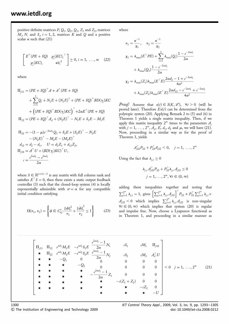
Note that ti , ti�1 therefore there exists a positive finiteinteger k(t) such that (see Fig. 1)
z2(t) ¼ (�Ad22)k(t)z2(tk(t))�
Xk(t)�1
i¼0
(�Ad22)iAd21z1(tiþ1) (18)
and tk(t) [ (�d2, 0]. Therefore from (11), (12), (16), Lemma2.2 and noting that
k(t)d2 � t, ti ¼ t �Xi�1
j¼0
d (tj) � t � id2
Figure 1 The relation between different ti, i ¼ 1, 2, . . . .
IET Control Theory Appl., 2009, Vol. 3, Iss. 9, pp. 1293–1305doi: 10.1049/iet-cta.2008.0212
IETdo
www.ietdl.org
we obtain
kz2(t)k � kAd22k(t)k f�� ��
cþ Ad21
�� �� Xk(t)�1
i¼0
Ad22i
�� ��kz1(tiþ1)k
� xe�ad2k(t)kfkc þ kAd21k
ffiffiffiffiffil2
l1
sf�� ��
c
�Xk(t)�1
i¼0
Ad22i
�� ��e�a(t�(iþ1)d2)
� x f�� ��
cþ Ad21
�� �� ffiffiffiffiffil2
l1
sead2 f
�� ��c
Xk(t)�1
i¼0
Ad22
�� ��ieiad2
" #e�at
� xþ Ad21
�� �� ffiffiffiffiffil2
l1
sead2 M
" #kfkce
�at
where
M ¼b
1� g, x ¼
ffiffiffiffiffiffiffiffiffiffiffiffiffiffiffiffiffiffiffiffiffilmax(Q322)
lmin(Q322)
s
Thus, the singular time-delay system is exponentially stablewith a minimum decaying rate ¼ a. Finally, as we haveshown that this system is also regular and impulse free, byDefinition 1, we then have that the system is exponentiallyadmissible. This completes the proof. A
Remark 1: Equation (18) can be seen as a generalisation ofthe iterative equation in [4] for systems with constant timedelay. Also, based on (11), which is equivalent to (20) in[4] as a goes to 0, the stability of the algebraic subsystemhas been shown for the case of time-varying delay. Thus,the results in [4], and in [5, 6] as well, can be extendedeasily to the case of time-varying delay.
Remark 2: It is noted that condition (6) is non-strict LMI,which contains equality constraints. This may result innumerical problems when checking such non-strict LMIconditions since equality constraints are fragile and usuallynot satisfied perfectly. Therefore strict LMI conditions aremore desirable than non-strict ones from the numericalpoint of view [19]. Considering this, (5) and (6) can becombined into a single strict LMI. Let P . 0 andS [ Rn�(n�r) be any matrix with full column rank andsatisfies E`S ¼ 0. Changing P to PE þ SQ in (5) yieldsthe strict LMI.
Now, the stabilisation problem of system (1) via staticoutput feedback controller will be addressed. The techniqueintroduced in [20] will be adopted in order to write thesaturated non-linear system (4) in a linear polytopic form.Let us write the saturation term as
sat(KCx(t)) ¼ D(r(x))KCx(t), D(r(x)) [ Rm�m
Control Theory Appl., 2009, Vol. 3, Iss. 9, pp. 1293–1305i: 10.1049/iet-cta.2008.0212
where D(r(x)) is a diagonal matrix for which the diagonalelements ri(x) are defined for i ¼ 1, . . . , m as
ri(x) ¼
�ui
(KC)ixif (KC)ix � �ui
1 if �ui , (KC)ix , ui
ui
(KC)ixif (KC)ix � ui
8>>>><>>>>:Using this, system (4) can be written as follows
E _x(t) ¼ (A þ BD(r(x))KC)x(t)þ Ad x(t � d (t)) (19)
The coefficient ri(x) can be viewed as an indicator of thedegree of saturation of the ith entry of the control vector.In fact, the smaller ri(x), the farther is the state vector fromthe region of linearity.
Let 0 , ri� 1 be a lower bound to ri(x), and define a
vector r ¼ [r1, . . . , r
m]. The vector r is associated to the
following region in the state space
S(K , ur) ¼ {x [ Rnj � ur � KCx � ur}
where every component of the vector u r is defined by ui=ri.
This vector can be viewed as a specification on thesaturation tolerance. Define now matrices Aj , j ¼ 1, . . . , 2m,as follows
Aj ¼ A þ BD(gj)KC
where D(gj) is a diagonal matrix of positive scalars gj(i) fori ¼ 1, . . . , m, which arbitrarily take the value one or r
i.
Note that the matrices Aj are the vertices of a convexpolytope of matrices. If x(t) [ S(K , ur), it follows that(A þ BD(r(x))KC) [ co{A1, . . . , A2m }. We conclude that ifx(t) [ S(K , ur), then E _x(t) can be determined from thefollowing polytopic model
E _x(t) ¼X2m
j¼1
lj,tAjx(t)þ Ad x(t � d (t)) (20)
withP2m
j¼1 lj,t ¼ 1 and lj,t � 0.
Remark 3: Different control saturation models areproposed in the literature, that is regions of saturation,differential inclusion and sector modelling. In [21], acomparative analysis of these models is presented, andconcluded that the differential inclusion model leads tothe least conservative design. Based on that, thedifferential inclusion model for the actuator saturation isused here.
Then we have the following result.
Theorem 2: Let 0 , d1 , d2, a . 0, a vector r and0 � m , 1 be given. If there exist symmetric and
1299
& The Institution of Engineering and Technology 2009
13
&
www.ietdl.org
positive-definite matrices P, Q1, Q2, Q3, Z1 and Z2, matricesMi, Ni and Si, i ¼ 1, 2, matrices K and Q and a positivescalar k such that (21)
E`(PE þ SQ) ri(KC)i
`
ri(KC)i kui
2
" #� 0, i ¼ 1, . . . , m (22)
where
Pj11 ¼ (PE þ SQ)`A þ A`(PE þ SQ)
þX3
i¼1
Qi þ N1E þ (N1E)`þ (PE þ SQ)`BD(gj)KC
þ (PE þ SQ)`BD(gj)KC `
þ2aE`(PE þ SQ)
P12 ¼ (PE þ SQ)`Ad þ (N2E)`� N1E þ S1E �M1E
P22 ¼ �(1� m)e�2ad2 Q3 þ S2E þ (S2E)`� N2E
� (N2E)`�M2E � (M2E)`
d12 ¼ d2 � d1, U ¼ d2Z1 þ d12Z2,
Pj18 ¼ A`U þ (BD(gj)KC)`U ,
c ¼e2ad2 � e2ad1
2a
where S [ Rn�(n�r) is any matrix with full column rank andsatisfies E`S ¼ 0, then there exists a static output feedbackcontroller (3) such that the closed-loop system (4) is locallyexponentially admissible with s ¼ a for any compatibleinitial condition satisfying
V(n1, n2) ¼ f [ Cvd2
:kfk2cn1
þk _fk
2
c
n2
� 1
( )ð23Þ
00The Institution of Engineering and Technology 2009
where
n1 ¼k�1
x1
, n2 ¼k�1
x2
x1 ¼ lmax(E`PE)þ
X2
i¼1
lmax(Qi)1� e�2adi
2a
þ lmax(Q3)1� e�2ad2
2a
x2 ¼ lmax(Z1)lmax(E`E)2ad2 � 1þ e�2ad2
4a2
þ lmax(Z2)lmax(E`E)
2ad12 � e�2ad1 þ e�2ad2
4a2
Proof: Assume that x(t) [ S(K , ur), 8t . 0 (will beproved later). Therefore E _x(t) can be determined from thepolytopic system (20). Applying Remark 2 to (5) and (6) inTheorem 1 yields a single matrix inequality. Then, if weapply this matrix inequality 2m times to the parameters Aj
with j ¼ 1, . . . , 2m, Ad , E, d1, d2 and m, we will have (21).Now, proceeding in a similar way as for the proof ofTheorem 1, yields
A`j22P22 þ P`
22Aj22 , 0, j ¼ 1, . . . , 2m
Using the fact that lj,t � 0
lj,t A`j22P22 þ P`
22lj,t Aj22 � 0
j ¼ 1, . . . , 2m, 8t [ (0, 1)
adding these inequalities together and noting thatP2m
j¼1 lj,t ¼ 1, givesP2m
j¼1 lj,t Aj22
h i`
P22 þ P`22
P2m
j¼1 lj,t�
Aj22 , 0 which impliesP2m
j¼1 lj,t Aj22 is non-singular
8t [ (0, 1) which implies that system (20) is regularand impulse free. Now, choose a Lyapunov functional asin Theorem 1, and proceeding in a similar manner as
Pj11 P12 ead1 M1E �ead2 S1E
w P22 ead1 M2E �ead2 S2E
w w �Q1 0
w w w �Q2
w w w w
w w w w
w w w w
w w w w
e2ad2 � 1
2aN1 cS1 cM1 Pj18
e2ad2 � 1
2aN2 cS2 cM2 A`
d U
0 0 0 0
0 0 0 0
�e2ad2 � 1
2aZ1 0 0 0
w �c(Z1 þ Z2) 0 0
w w �cZ2 0
w w w �U
26666666666666666664
37777777777777777775
, 0 j ¼ 1, . . . , 2m (21)
IET Control Theory Appl., 2009, Vol. 3, Iss. 9, pp. 1293–1305doi: 10.1049/iet-cta.2008.0212
IETdo
www.ietdl.org
before, then
_V (t)þ 2aV (t) � h`(t)
"PþeA`
(d2�Z1 þ d12
�Z2)eAþ
e2ad2 � 1
2aeN �Z
�1
1eN `
þe2ad2 � e2ad1
2aeS �Z1 þ
�Z2
� ��1eS`
þe2ad2 � e2ad1
2aeM �Z
�1
2eM`
#h(t)
with all the variables as defined in Theorem 1 and A isreplaced by
P2m
j¼1 lj,tAj . Then, by convexity and notingthat
P2m
j¼1 lj,t ¼ 1 with lj,t � 0, condition (21) yields
_V (t)þ 2aV (t) � 0
The rest of the proof is similar to the proof of Theorem 1,and the details are omitted.
Now, by virtue of condition (22), the ellipsoid defined byG ¼ {x [ Rn : x`E`(PE þ SQ) x � k�1} is included in theset S(K , ur) [20]. Suppose now that the initial conditionf(t) satisfies (23), and conditions (21) and (22) hold.Then, from the definition of V (t), it follows thatx`(0) E`(PE þ SQ)x(0) � V (0) � x1kfk
2c þ x2k
_fk2c � k�1
and, in this case, one has x(0) [ G , S. Now, since_V (0) , 0, we conclude that x`(t)E`(PE þ SQ)x(t) �V (t) � V (0) � x1kfk
2cþ x2k
_fk2
c � k�1, which means thatx(t) [ S(K , ur), 8t . 0. This completes the proof. A
Remark 4: Being inside the set V(n1, n2), thecompatibility of the initial condition is also very importantespecially when saturation is present. It is well knownthat incompatible initial conditions results in jumpdiscontinuities because of the singular structure. Such jumpdiscontinuities may take the system outside the setV(n1, n2), where the controller may be unable to stabilisethe system.
It is obvious that (21) is a bilinear matrix inequality (BMI),and consequently its solution is very difficult. Thus, aniterative LMI (ILMI) approach similar to [22, 23] will beproposed. The derivation of the algorithm is similar to [22,23] and will be omitted. This algorithm has the samedisadvantages as those in [22, 23], that is based on asufficient conditions. The following is the proposedalgorithm and the explanation is given later.
ILMI algorithm
Control Theory Appl., 2009, Vol. 3, Iss. 9, pp. 1293–1305i: 10.1049/iet-cta.2008.0212
Step 1: OP1
minP0.0,Q,Q1.0,Q2.0,Q3.0,Zp0.0,Mp,Np ,Sp ,p¼1,2,k
b0
s.t. (26) and (27)
K ¼ 0 and X0 ¼ E
Set i ¼ 1, X1 ¼ E, Z11 ¼ Z10 and Z21 ¼ Z20.
Step 2: OP2
minPi.0,Q,Q1.0,Q2.0,Q3.0,Mp,Np,Sp,p¼1,2,K ,k
bi
s.t. (26) and (27)
Let bi� and K � be the solution of OP2. If bi
�� �a, where
a is a prescribed decay rate, then K � is a stabilising staticoutput feedback gain, go to step 5, otherwise, go to step 3.
Step 3: OP3
minPi.0,Q,Q1.0,Q2.0,Q3.0,Zpi.0,Mp ,Np,Sp,p¼1,2,k
tr(E`Ti)
s.t. (26) and (27)
bi ¼ b�i and K ¼ K �
If kXiB � T �i Bk , e, go to step 4, else set i ¼ i þ 1, Xi ¼
T �i�1, Z1i ¼ Z�1(i�1) and Z2i ¼ Z�2(i�1), then go to step 2.
Step 4: The system may not be stabilisable via static outputfeedback. Stop.
Step 5: OP4
minP.0,Q,Q1.0,Q2.0,Q3.0,Zp.0,Mp,Np,Sp,p¼1,2,K ,k
r
s.t.(26) and (27), bi ¼ a
d1I � E`PE, d2I � Q1; d3I � Q2 (24)
d4I � Q3, d5I � Z1, d6I � Z2 (25)
where
r ¼ w1 d1 þ1� e�2ad1
2ad2 þ
1� e�2ad2
2ad3 þ
1� e�2ad2
2ad4
!
þw2 lmax(E`E)
2ad2 � 1þ e�2ad2
4a2d5
þlmax(E`E)
2ad12 � e�2ad1 þ e�2ad2
4a2d6
!þw3k, and w1, w2 and w3 are weighting factors.
1301
& The Institution of Engineering and Technology 2009
13
&
www.ietdl.org
We solve this problem iteratively in two steps as follows:
(a) Fix K, and solve for P . 0, Q, Q1 . 0,Q2 . 0, Q3 . 0, Zp . 0, Mp, Np, Sp, p ¼ 1, 2, and k.
(b) Fix Z1 and Z2, and solve for P . 0, Q, Q1 . 0,Q2 . 0, Q3 . 0, Mp, Np, Sp, p ¼ 1, 2, K and k. Set X ¼ T .
The set (23) is calculated from the matrices that solve OP4(see (26))
E`Ti rr(KC)r
`
rr(KC)r kur
2
" #� 0, r ¼ 1, . . . , m (27)
where
P11 ¼ T `i A þ A`Ti þ
X3
i¼1
Qi þ N1E þ (N1E)`
� XiBB`Ti � (XiBB`Ti)`þ XiBB`Xi � 2biE
`Ti
Pj18 ¼ A`U þ (BD(gj)KC)`U
P22 ¼ �(1� m)e2bd (b)Q3 þ S2E þ (S2E)`� N2E
� (N2E)`�M2E � (M2E)`
Ti ¼ (PiE þ SQ), d (b) ¼d1 if b . 0
d2 if b , 0
and the other variables as defined previously.
Remark 5: The core of this algorithm is in OP2 and OP3.As shown in [22], OP2 guarantees the progressive reduction ofbi whereas OP3 guarantees the convergence of the algorithm.Yet, in [22], only X needs to be fixed in order to obtain LMIs,whereas in our case, we have also to fix either Z1 and Z2 or Kto obtain LMIs. Thus, we will fix Z1 and Z2 in OP2, and K inOP3. This way of solving this problem will not affect theconvergence of the algorithm. It is worth noting thatalthough this ILMI algorithm is convergent, we may not
02The Institution of Engineering and Technology 2009
achieve the solution because b may not always converge toits minimum. For more details on the numerical propertiesof the algorithm, we refer the reader to [22].
Remark 6: In order to start the algorithm, OP2 should havea solution for i ¼ 1. Yet, the solution depends on the initialmatrix X. In [23], some Riccati equation is proposed in orderto select an initial X for the descriptor version of thisalgorithm. In [24], it has been proved that this Riccatiequation may not have a solution and an initial value ofX ¼ I is proposed instead. Actually, the identity matrixmay not do the job for even some simple systems, anexample of such systems is
(A, B, C) ¼ (I, I, I), E ¼I 00 0
� �Our numerical experience indicates that an initial choice ofX0 ¼ E often leads to a convergent result. With this X0,OP1 is used here to obtain initial values for Z1 and Z2.
Remark 7: The minimisation of b in OP1 and OP2 shouldbe done using the bisection method. The lower bound of thebisection method can be any value less than 2a since we arenot interested in minimising b less than 2a. The upperbound of the bisection method can be any sufficiently largenumber. These upper and lower bounds should be chosenonly once and can be fixed throughout the algorithm.
Remark 8: OP4 is used in order to enlarge the set ofinitial conditions (23). The satisfaction of (24) and (25)means that x1 � d1 þ [(1� e�2ad1 )=2a]d2 þ [(1� e�2ad1 )=2a]d3 þ [(1� e�2ad1 )=2a]d4 and x2 � lmax(E`E)[(2ad2�
1þ e�2ad2 )=4a2] d5 þ lmax(E`E)[(2ad12 � e�2ad1 þ
e�2ad2 )=4a2]d6. Therefore because ni ¼ k�1=xi, if weminimise the criterion as defined in OP4, then greater thebounds on kfk2
c and k _fk2c tend to be. In other words, byusing OP4, we orient the solutions of LMIs (21) and (22)in a sense to obtain the set V(n1, n2) as large as possible.For more discussion on this topic, we refer the reader to [20].
P11
(B`Ti
þD(gj )KC)`
" #P12 e�bi d1 M1E �e�bi d2 S1E
e�2bi d2 � 1
�2bi
N1
e�2bi d2 � e�2bi d1
�2bi
S1
e�2bi d2 � e�2bi d1
�2bi
M1 Pj18
(B`Ti
þD(gj )KC)
" #�I 0 0 0 0 0 0 0
w 0 P22 e�bi d1 M2E �e�bi d2 S2Ee�2bi d2 � 1
�2bi
N2
e�2bi d2 � e�2bi d1
�2bi
S2
e�2bi d2 � e�2bi d1
�2bi
M2 Ad`U
w 0 w �Q1 0 0 0 0 0
w 0 w w �Q2 0 0 0 0
w 0 w w w �e�2bi d2 � 1
�2bi
Z1i 0 0 0
w 0 w w w w �e�2bi d2 � e�2bi d1
�2bi
(Z1i þ Z2i) 0 0
w 0 w w w w w �e�2bi d2 � e�2bi d1
�2bi
Z2i 0
w 0 w w w w w w �U
26666666666666666666666666666664
37777777777777777777777777777775, 0 j ¼ 1, . . . , 2m (26)
IET Control Theory Appl., 2009, Vol. 3, Iss. 9, pp. 1293–1305doi: 10.1049/iet-cta.2008.0212
IET Control Theory Appl., 2009,doi: 10.1049/iet-cta.2008.0212
www.ietdl.org
Table 1 Maximum allowable decay rates a for different d2 withd1 ¼ 0.2 and m ¼ 0.5
d2 0.5 0.6 0.7 0.8 0.9 1 1.1
a 0.3239 0.3014 0.2816 0.2642 0.2411 0.1323 0.0290
4 Examples4.1 Example 1
Consider the singular time-delay system studied in [5] with
E ¼1 00 b
� �, A ¼
0:5 0�1 �1
� �, Ad ¼
�1 00 0
� �Let b ¼ 0, we know from [5] that this system is asymptoticallystable for constant delay t , t� and unstable for constant delayt . t�, where t� ¼ 1:2092. Now, allowing time-varying delay,the exponential stability of this system will be investigated using
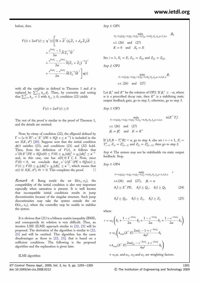
Figure 2 Simulation results of x1 and x2 as compared toe20.3t
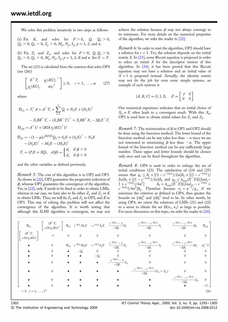
Figure 3 Simulation results of x1, x2 and x3
Vol. 3, Iss. 9, pp. 1293–1305
Theorem 1. For various d2, the maximum allowable decay ratesa, which guarantee the exponential stability for given lowerbound d1 and derivative bound m, are listed in Table 1. As itis clear from the table, if we increase d2, then we obtainsmaller decay rates a. Fig. 2 gives the simulation results of x1
and x2 as compared to e�0:3t when d (t) ¼ 0:4þ 0:1 sin(4t)and the initial function is f(t) ¼ [1 �1]`, t [ [�0:4, 0].From Fig. 2, we can see that the states x1 and x2
exponentially converge to zero with a decay rate greater than0.3. Now, let b ¼ 0:5 (i.e. the delay appear also in thealgebraic constraint). For d1 ¼ 0:2, d2 ¼ 0:5 and m ¼ 0:5,the maximum allowable decay rate is a ¼ 0:32.
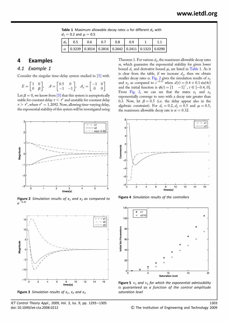
Figure 4 Simulation results of the controllers
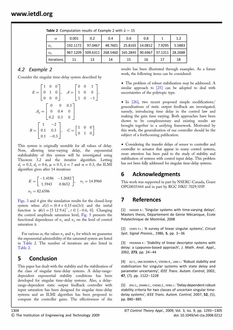
Figure 5 n1 and n2 for which the exponential admissibilityis guaranteed as a function of the control amplitudesaturation level
1303
& The Institution of Engineering and Technology 2009
1304
& The Institution of
www.ietdl.org
Table 2 Computation results of Example 2 with u ¼ 15
a 0.001 0.2 0.4 0.6 0.8 1 1.2
n1 192.1172 97.0467 48.7601 25.8165 14.0812 7.9295 5.5883
n2 967.1209 509.6311 268.5460 165.2845 90.6967 37.1311 28.2688
iterations 11 13 14 15 16 17 18
4.2 Example 2
Consider the singular time-delay system described by
E ¼
1 0 0
0 1 0
0 0 0
264375, A ¼
0 0 1
1 0 0
1 0 �1
264375,
Ad ¼
0 0 0:3
0 0:4 0
0:2 0:3 0
264375
B ¼
1 �2
0:1 0:3
0:1 �0:3
264375, C ¼
1 0 0
0 1 0
� �
This system is originally unstable for all values of delay.Now, allowing time-varying delay, the exponentialstabilisability of this system will be investigated usingTheorem 3.2 and the iterative algorithm. Lettingd1 ¼ 0:2, d2 ¼ 0:6, m ¼ 0:5, u ¼ 7 and a ¼ 0:3, the ILMIalgorithm gives after 14 iterations
K ¼�1:4186 �1:2682
1:3943 0:8652
� �, n1 ¼ 14:8960
n2 ¼ 82:6586
Figs. 3 and 4 give the simulation results for the closed-loopsystem when d (t) ¼ j0:4þ 0:15 sin(3t)j and the initialfunction is f(t) ¼ [5 12 9:6]`, t [ [�0:6, 0]. Changingthe control amplitude saturation level, Fig. 5 presents thefunctional dependence of n1 and n2 on the level of controlsaturation u.
For various a, the values n1 and n2 for which we guaranteethe exponential admissibility of the saturated system are listedin Table 2. The number of iterations are also listed inTable 2.
5 ConclusionThis paper has dealt with the stability and the stabilisation ofthe class of singular time-delay systems. A delay-range-dependent exponential stability conditions has beendeveloped for singular time-delay systems. Also, a delay-range-dependent static output feedback controller withinput saturation has been designed for singular time-delaysystems and an ILMI algorithm has been proposed tocompute the controller gains. The effectiveness of the
Engineering and Technology 2009
results has been illustrated through examples. As a futurework, the following items can be considered:
† The problem of robust stabilisation may be addressed. Asimilar approach to [25] can be adopted to deal withuncertainties of the polytopic type.
† In [26], two recent proposed simple modifications/generalisations of static output feedback are investigated;namely, introducing time delay in the control law andmaking the gain time varying. Both approaches have beenshown to be complementary and existing results arebrought together in a unifying framework. Motivated bythis work, the generalisation of our controller should be thesubject of a forthcoming publication.
† Considering the transfer delays of sensor to controller andcontroller to actuator that appear in many control systems,more attention has been paid to the study of stability andstabilisation of systems with control input delay. This problemhas not been fully addressed for singular time-delay systems.
6 AcknowledgmentsThis work was supported in part by NSERC-Canada, GrantOPG0035444 and in part by RGC HKU 7029/05P.
7 References
[1] HAIDAR A.: ‘Singular systems with time-varying delays’.Masters thesis, Departement de Genie Mecanique, EcolePolytechnique de Montreal, 2008
[2] LEWIS F.L.: ‘A survey of linear singular systems’, CircuitSyst. Signal Process., 1986, 5, pp. 3–36
[3] FRIDMAN E.: ‘Stability of linear descriptor systems withdelay: a Lyapunov-based approach’, J. Math. Anal. Appl.,2002, 273, pp. 24–44
[4] XU S., VAN DOOREN P., STEFAN R., LAM J.: ‘Robust stability andstabilization for singular systems with state delay andparameter uncertainty’, IEEE Trans. Autom. Control, 2002,47, (7), pp. 1122–1228
[5] ZHU S., ZHANG C., CHENG Z., FENG J.: ‘Delay-dependent robuststability criteria for two classes of uncertain singular time-delay systems’, IEEE Trans. Autom. Control, 2007, 52, (5),pp. 880–885
IET Control Theory Appl., 2009, Vol. 3, Iss. 9, pp. 1293–1305doi: 10.1049/iet-cta.2008.0212
IETdoi
www.ietdl.org
[6] FENG J., ZHU S., CHENG Z.: ‘Guaranteed cost control oflinear uncertain singular time-delay systems’. Conf.Decision and Control, 2002
[7] YUE D., LAM J., HO D.W.C.: ‘Delay-dependent robustexponential stability of uncertain descriptor systems withtime-varying delays’, Dyn. Continuous Discrete ImpulsiveSyst. B, 2005, 12, (1), pp. 129–149
[8] HE Y., WU M., SHE J.-H., LIU G.-P.: ‘Parameter-dependentLyapunov functional for stability of time-delay systemswith polytopic-type uncertainties’, IEEE Trans. Autom.Control, 2004, 49, (5), pp. 828–832
[9] WU M., HE Y., SHE J.-H., LIU G.-P.: ‘Delay-dependent criteriafor robust stability of time-varying delay systems’,Automatica, 2004, 40, pp. 1435–1439
[10] XU S., LAM J.: ‘Improved delay-dependent stabilitycriteria for time-delay systems’, IEEE Trans. Autom.Control, 2005, 50, (3), pp. 384–387
[11] HE Y., WANG Q.-G., LIN C., WU M.: ‘Delay-range-dependentstability for systems with time-varying delay’, Automatica,2007, 43, pp. 371–376
[12] SUN Y.-J.: ‘Exponential stability for continuous-timesingular systems with multiple time delays’, J. Dyn. Syst.Meas. Control, 2003, 125, (2), pp. 262–264
[13] BERNSTEIN D.S., MICHEL A.N.: ‘A chronological bibliographyon saturating actuators’, Int. J. Robust Nonlinear Control,1995, 5, pp. 375–380
[14] LAN W., HUANG J.: ‘Semiglobal stabilization and outputregulation of singular linear systems with inputsaturation’, IEEE Trans. Autom. Control, 2003, 48, (1),pp. 1274–1280
[15] CASTALAN E.B., SILVA A.S., VILLARREAL E.R.L., TARBOURIECH S.:‘Regional pole placement by output feedback for a classof descriptor systems’. IFAC 15th Triennial WorldCongress, Barcelona, Spain, 2002
[16] KUO C.-H., FANG C.-H.: ‘An LMI approach toadmissibilization of uncertain descriptor systems via static
Control Theory Appl., 2009, Vol. 3, Iss. 9, pp. 1293–1305: 10.1049/iet-cta.2008.0212
output feedback’. Proc. American Control Conf., Denver,Colorado, 4–6 June 2003
[17] BOUKAS E.K.: ‘Delay-dependent static output feedbackstabilization for singular linear systems’. Les Cahiers duGERAD 2004, HEC Montreal G200479
[18] KHARITONOV V., MONDIE S., COLLADO J.: ‘Exponentialestimates for neutral time-delay systems: an LMIapproach’, IEEE Trans. Autom. Control, 2005, 50, (5),pp. 666–670
[19] XU S., LAM J.: ‘Robust control and filtering of singularsystems’ (Springer, 2006)
[20] TARBOURIECH S., GOMES DA SILVA JR. J.M.: ‘Synthesis ofcontrollers for continuous-time delay systems withsaturating controls via LMI’s’, IEEE Trans. Autom. Control,2000, 45, (1), pp. 105–111
[21] GOMES DA SILVA JR J.M., TARBOURIECH S., REGINATTO R.:‘Conservativity of ellipsoidal stability regions estimates forinput saturated linear systems’. 15th Triennial WorldCongress, Barcelona, Spain, 2002
[22] CAO Y.Y., LAM J., SUN Y.X.: ‘Staticoutput feedback stabilization: an ILMI approach’,Automatica, 1998, 34, (12), pp. 1641–1645
[23] ZHENG F., WANG Q.-G., LEE T.H.: ‘On the design ofmultivariable PID controllers via LMI approach’,Automatica, 2002, 38, (3), pp. 517–526
[24] LIN C., WANG Q.-G., LEE T.H.: ‘An Improvement onmultivariable PID controller design via iterative LMIapproach’, Automatica, 2004, 40, pp. 519–525
[25] TARBOURIECH S., GARCIA G., GOMES DA SILVA J.M.: ‘Robuststability of uncertain polytopic linear time-delay systemswith saturating inputs: an LMI approach’, Comput. Electr.Eng., 2002, 28, (3), pp. 157–169
[26] MICHIELS W., NICULESCU S.-I., MOREAU L.: ‘Using delays andtime-varying gains to improve the static output feedbackstabilizability of linear systems: a comparison’, IMAJ. Math. Control Inf., 2004, 21, (4), pp. 393–418
1305
& The Institution of Engineering and Technology 2009
Recommended


