Download pdf - Government Spending and Air Pollution in the US

Department of Agricultural and Resource Economics

The University of Maryland, College Park

Copyright 2013 by Asif M. Islam and Ramón E. López All rights reserved. Readers may make verbatim copies of this document for non-commercial purposes by any means, provided that this copyright notice appears on all such copies.

Government Spending and

Air Pollution in the US

by

Asif M. Islam and Ramón E. López

WP 13-02

Government Spending and Air Pollution in the US

Asif M. Islam* University of Maryland

2106 Symons Hall College Park, MD 20740

(651) 246 4017 [email protected]

Ramón E. López University of Maryland

3125 Symons Hall College Park, MD 20740

(301) 405 1281 [email protected]

JEL Classification: H50, H40, O13, O44, Q53

Keywords: air pollution, government spending, public goods, market imperfections

*Corresponding author, Fax: (301) 314 9091

mailto:[email protected]

mailto:[email protected]

1

Government Spending and Air Pollution in the US

Abstract

This study examines the effect of the composition of federal and state government spending on various important air pollutants in the US using a newly assembled data set of government expenditures. The results indicate that a reallocation of spending from private goods (RME) to social and public goods (PME) by state and local governments reduces air pollution concentrations while the composition of federal spending has no effect. A 10 percent increase in the share of social and public goods spending by state and local governments reduces air pollution concentrations by 3 to 5 percent for Sulfur Dioxide, 2 to 3 percent for Particulate Matter 2.5 and 1 to 2 percent for Ozone. The results are robust to various sensitivity checks.

1. Introduction Much attention has been awarded to the arsenal of regulatory policy tools at the disposal of the

US policy makers addressing environmental concerns. However, while many efforts have been

devoted to study the effects of various economy-wide policies (most prominently trade policies)

on the environment, little analysis has been done on the impact of other important economy-wide

policies such as fiscal spending policies on environmental outcomes. This is surprising in view

of the massive importance of government spending in the US economy. Furthermore, not much

consideration has been given to the possible variation of fiscal policy impacts by the level of

government. This paper explores the environmental implications when a government embarks

on broad fiscal policy changes, altering the composition of government expenditures towards

increasing the provision of social and public goods (PME spending) at the cost of private

subsidies (RME spending) in order to correct market imperfections. The impact of compositional

changes in spending is examined at two levels of government: federal government spending and

combined state & local government spending. This link between of fiscal policy and the

environment is important particularly because the 2008-2009 financial crisis has put US fiscal

policy in the forefront of much debate and scrutiny especially with regards spending priorities.

This paper specifically investigates the impact of US government spending on sulfur dioxide

(SO2), particulate matter 2.5 (PM2.5 - particulate matter of diameter size 2.5 microns or smaller)

and ozone (O3) concentrations for the time periods 1985-2008, 2000-2008, and 1983-2008

2

respectively1. We study the effects of the size of fiscal expenditures and of a reallocation of

spending from RME to PME at the state and local level as well as federal level using for the first

time a new panel dataset of government expenditures spanning all states, covering the time

period of 1983 to 2008, recently developed by Islam (2011).

We find that shifting the composition of local and state expenditures from RME to PME reduces

air pollution concentrations of the three pollutants considered, while the composition of federal

spending has no effect. Furthermore, the size of the state and local public sector expenditures has

no significant effect on pollution. Total federal spending does have a significant effect on

pollution but the sign of the effect is not robust. We find that a 10 percent increase in the share of

state and local PME spending reduces air pollution concentrations by the range of 3 to 5 percent

for Sulfur Dioxide, 2 to 3 percent for Particulate Matter 2.5 and 1 to 2 percent for Ozone. The

results are robust to various sensitivity checks2.

This study adds to a long literature that has examined the determinants of air pollutants in the US

(List and Gallet, 1999; Khanna, 2002). A few studies have examined the impact of the 1990

Clean Air Act Amendments (CAAA) on PM10 concentrations (Aufhammer et al., 2009;

Aufhammer et al.,2011), Ozone (Henderson, 1996), SO2 concentrations directly (Carlson et. al,

2000; Greenstone, 2004), as well as indirectly by examining the impact of 1990 CAAA on input

substitution from high-sulfur to low-sulfur coal by utility plants (Gerking and Hamilton, 2010).

In addition to regulation, community characteristics have also been found to be significant

determinants of pollutants (Brooks and Sethi, 1997). In the wider literature there are several

studies that have also explored the cross-country determinants of pollutants, specifying various

1 The focus on SO2, PM2.5, and O3 is justified for several reasons. The data on these pollutants are available for a large period of time, especially for ozone and sulfur dioxide air concentrations. The adverse health effects of each of the three pollutants are well documented. Also since industrial activity is a significant contributor to SO2, PM 2.5 and Ozone air concentrations, the wide range of output elasticities in the literature for energy from a low of 0.01 to a high of 1.035 (Kamerschen and Porter, 2004; Liu, 2004) implies that we expect macro-economic factors to have an impact on the air pollution concentrations. For a full list of output elasticity measures see Table B7 in the online appendix (http://ter.ps/envappendix). 2 An alternate approach to the current study would be use CGE models as carried out in the literature (Jorgenson and Wilcoxen, 1990). However, CGE models depend upon strong assumptions and lack of data precludes econometric estimation of key supply and demand parameters. Also, CGE models are more effective for global than local pollutants (Bergman, 2005).

http://ter.ps/envappendix

3

mechanisms linking macro-economic factors such as income and trade to environmental

outcomes (Shafik and Bandhopadhyay, 1992; Grossman and Krueger, 1995; Barrett and Grady,

2000, Antweiler, Copeland and Taylor, 2001; Frankel and Rose, 2005; Bernauer and Koubi,

2006; Deacon and Norman, 2007;).

This study builds on López, Galinato, and Islam (2011), which explores a similar relationship

between government spending composition and pollution across countries. Limitations of López,

Galinato, and Islam (2011) include difficulty in accounting for regulation in cross-country

studies, highly aggregated spending data, and no distinction between the sources of the

government expenditures. In addition, López, Galinato, and Islam (2011) only explore the

relationship between government spending and production based pollutants while we also

consider consumption based pollutants which has important implications (McAusland, 2008).

The contributions of this study to the literature can be summarized as follows (i) quantifying the

relationship between US fiscal spending composition and air pollution using a newly developed

highly disaggregated fiscal spending data set, (ii) exploring the difference in the impact of fiscal

policy by the level of government, and (iii) using a new estimation method that accounts for time

varying omitted variable bias using state specific polynomials of a time trend that exploit the

available degrees of freedom. This estimation generalizes similar estimations that have been used

in the literature (Cornwell et al., 1990; Jacobsen et al., 1993; Friedberg, 1998; Wolfers, 2006).

The paper is structured as follows. Section 2 provides an overview of SO2, PM 2.5, and O3

pollution sources and regulations implemented in the US. Sections 3, 4, 5, 6, 7 and 8 provide

conceptual issues, econometric model, data description, results, robustness, and conclusions

respectively.

2. Air Pollution Sources and Regulation Table A6 presents the sources of the SO2 and PM2.5 emissions, and the O3 precursor pollutant

emissions - NO and VOC. About 67% of SO2 emissions originate from fuel combustion in

electric utilities, while another 23% is from Industrial fuel combustion and processes. The largest

contributor towards PM 2.5 emissions is fugitive dust accounting for about 41% of overall

4

emissions. Industrial fuel combustion and processes contribute around 14% of PM 2.5 emissions

with forest and agricultural wildfires contributing about 13% and agricultural crops and livestock

contributing another 13%. NO and VOC combine to form ground level O3, however the sources

of their emissions differ in some respects. Both pollutants have transportation - both on-road and

non-road vehicles as a significant source contributing 53% of NO and 44% of VOC emissions.

However, although 25% and 16% of NO emissions are from electric utilities and industrial

activities respectively, for VOCs, 47% comes from industrial activities with about 0.2%

originating from electric utilities.

Air pollution regulation in the US comes in the form of air quality standards and Cap-and-Trade

programs for certain pollutants. Initially air pollution regulation in the United States was under

state and local government jurisdiction. The Clean Air Act in 1963, followed by the Air Quality

Act of 1967 provided funds from the federal government to state and local governments for

support and regulation of air pollution. However, the lack of enforcement and several delays in

formulating standards by states led to the Clean Air Act Amendments (CAAA) of 1970. This

engendered the EPA as well as the National Ambient Air Quality Standards (NAAQS), signaling

federal involvement in air pollution control in the US. National air quality standards were

published for six pollutants: Sulfur oxides, particulate matter, carbon monoxide, photochemical

oxides (ground level ozone), nitrogen oxides, and hydrocarbons (mostly via ozone standards). A

whole county violation occurs if all the monitoring sites in a county exceeded the standard air

pollution concentrations, while a partial violation was where only some of the air pollution

monitors in the county exceeded the standards. A county that violated the standard is assigned a

“non-attainment” status. In this case, states were required to submit a state implementation plan

(SIP) that indicated how the state planned to meet these standards. If the standards are still not

met, the EPA can impose sanctions that may include holding of federal highway funds.

The 1990 Amendments of the Clean Air Act involved more stringent air quality standards and

the creation of the Acid Rain Program (Title IV). In order to regulate acid deposition (acid rain) a

two stage emission strategy was imposed to reduce sulfur dioxide and nitrous oxides produced

from electric utilities. Phase I, implemented in 1995, involved issuing allowances to power

plants, which resulted in fines if exceeded. Phase II (began in 2000) imposed tighter caps on

5

phase I plants while emission limits were imposed on cleaner smaller plants. Permits were

allowed to be traded and thus the term, Cap and Trade.

3. Conceptual Issues In this section we provide a detailed explanation of the spending dichotomy used in this study.

We then sketch out the mechanisms by which the compositional shifts in government spending

may affect environmental outcomes.

3.1 Spending Categories

The rationale for the government spending categories is based on the presence of credit market

failures, positive human capital externalities, and environmental externalities. Productive and

wasteful government spending are distinguished by creating two categories – government

spending on market-promoting goods (PME) and spending on market restricting goods (RME).

PME spending addresses the market failures and externalities prevalent and thus encompass pure

public goods, which are non-rival and non-excludable, and social spending including

government expenditures on health, education, affordable housing, social welfare, environment,

and research and development expenditures. The private sector under-invests in R & D activities,

which generate positive externalities, and also has little incentives to spend in environmental

protection, which faces substantial market failures (Hoff and Stiglitz, 2000; Dasgupta, 1996)3.

PME expenditures tend to complement rather than substitute private investments and also

mitigate the effects of market failures, especially credit market failures, which affect a large

number of households (Attanasio et. al., 2008; Grant, 2007; Jappelli 1990; Zeldes, 1989). Social

subsidies specifically may alleviate liquidity constraints faced by households and therefore

increase investment in education and health, which have large positive externalities but tend to

be underinvested in (Galor and Zeira, 1993). Conventional public goods, such as legal

institutions including law and order are typically underinvested by the private sector, and thus

government spending in such activities is merited.

3 There is a possibility that public R&D spending may crowd out private R&D spending. However, overall this literature is not conclusive and the results are ambiguous (David et al., 2000).

6

RME spending usually fall under “development” or “economic affairs” expenditures that involve

subsidies directly to firms for activities such as product promotion, commodity market subsidies,

grants to corporations, bailouts of failed private financial institutions, and several others. Such

expenditures typically tend to promote capital-intensive industries, or substitute private

investment as they are typically captured by large corporations, which are typically financially

unconstrained (Slivinski, 2007). The costs and ineffectiveness of subsidies that fall under RME

spending has been well documented (Coady et. al. 2006)4. Furthermore, the availability of RME

spending tends to promote directly unproductive, profit-seeking activities (DUP) such as

lobbying, by mainly special interest groups. RME spending tends to elicit more rent-seeking

activities as firms are fewer than households, and can be grouped by production activity and thus

can more easily solve the collective action problem (López and Islam, 2011). Thus RME

expenditures are deemed as wasteful spending. The classification presented here is not novel and

has been presented in the literature (López, Galinato, and Islam 2011; López and Galinato,

2007). It is also important to note that since this study is exploring the implications of broad

fiscal spending policy on the environment, not all specific spending items need to have a direct

link to the environment.

3.2 Mechanisms

The channels through which the reallocation of spending from RME to PME affects air pollution

are conditional on whether pollution is generated from production or consumption activities

(McAusland, 2008). López et al. (2011) provide the theoretical background for identifying the

channels by which the level and composition of government spending may affect production-

generated pollutants. The reallocation of government expenditure from RME to PME goods may

trigger: (i) a scale effect where the increase in aggregate output results in greater pollution, (ii)

composition effect where the human capital-intensive nature of PME spending and the physical

capital-intensive nature of RME spending implies that a reallocation from RME to PME

spending may alter the composition of the economy towards cleaner human capital-intensive

sectors resulting in less pollution, and (iii) increased investments in R&D and knowledge

diffusion via PME spending may trigger a technique effect where cleaner technologies may be

developed. 4 For example the Savings and Loans crisis of the 1980s is estimated to have directly cost US taxpayers $150 billion over the period 1989-1992 (Curry and Shibut, 2000).

7

An increase in PME spending also affects consumption-based pollutants. It may change the

composition of consumption goods, as consumption is shifted towards less polluting goods. For

example, increasing PME spending may result in greater investments in public transportation,

resulting in consumers altering their preferences away from private forms of transportation that

are typically energy intensive, and thus reduce air pollution emissions (Shapiro et al., 2004;

Zimmerman, 2005). Increasing the share of PME spending may also increase R&D promoting

the consumption of more energy saving goods such as energy saving bulbs and energy saving

AC and heating units and others. Increases in human capital may heighten pollution awareness

among the general public resulting in a decrease in pollution intensive activities (McConnell,

1997). Using household surveys in Netherlands, Ferrer-i-carbonell et al., (2004), finds that

increasing public awareness of pollution changes consumer expenditures towards more

sustainable consumption. Such a reallocation of spending may also alter the consumption mix

towards less pollution-intensive goods making pollution abatement easier (see Seldon and Song,

1995; Orecchia and Tessitore, 2011).

3.3 Federal versus Local Spending

The impact of fiscal spending on environmental outcomes may have diverging effects depending

on the level of the government carrying out the policy. There are certain differences in

characteristics of federal versus state and local government that may result in differences in the

effectiveness of changes in the composition of fiscal spending. This includes differences in

bureaucracy or red tape, technical knowledge, flexibility to experiment with policy,

accountability to voters, and finally the ability to deal with race-to-the-bottom scenarios.

Given the divergence in size between federal and state government, the former tends to have a

larger degree of red tape and bureaucracy than the latter. This in turn leads to a lower degree of

flexibility in policy experimentation and also lower responsiveness of the federal government in

comparison to the smaller state and local governments. However federal governments may have

the technical expertise to carry out fiscal policy. Oates (2001) argues that in terms of

environmental policy, federal government involvement should mainly entail subsidies for

8

abatement technology, research and development, and information dissemination. Furthermore,

state governments may face soft budgets in anticipation of federal bailouts.

One concern is the potential for race to the bottom scenarios when state or local government

carry out fiscal policy. For instance, state governments may have disincentives to provide social

programs given the open nature of their economies due to the fear that they may attract poor

individuals and thus limiting their tax revenue base (Oates, 1999). Thus it is also likely that state

level governments may engage in spending that is more likely to attract businesses. Competition

to attract firms may induce greater RME spending and thus lead to race to the bottom scenarios.

It is important to note that the goal of broad fiscal policy is not necessarily to improve

environmental outcomes. Thus conclusions about the efficiency of broad fiscal spending cannot

be drawn from any positive or negative effect of fiscal policy on environmental outcomes. The

main concern is that specific inefficiencies in particular government spending programs may

affect the mechanisms by which broad fiscal policy affects environmental outcomes.

4. Econometric Model We establish the long run relationship between the stocks of government provided goods and air

pollution. We posit that pollution concentrations, jstZ , at monitoring site j , state s , averaged

over year t , are determined by the stocks of private (RME), and social and public goods (PME)

provided by the local government ( STstG ) and federal government ( FD

stG ), and a vector of regulations

( R st ). Given the importance of regulations, we will expand in detail on the elements of the vector

of regulations towards the end of the section (subsection 4.2). Additional controls include

monitoring site characteristics ( jstX ) and permanent income ( stI ) which consistent with the

literature, we proxy using a 3 year moving average of personal income (Antweiler, Copeland,

and Taylor, 2001). Finally, the estimation controls for monitoring site effects and unobserved

fixed and time varying state effects.

(1) 1 2 3 4 5R ( )ST FDjst js st st st st jst t st jstZ a G a G a I a a X tµ τ ϕ ε= + + + + + + + +

{ }1,2,......., ,j J∈ { }1,2,......., ,s S∈ { }1,2,......., ,t T∈

9

jsµ is the monitoring site effect that can be either fixed or random. ( )sttϕ is a function of time that

controls for fixed and time-varying state-specific effects; tτ are the year fixed effects and jstε is

an idiosyncratic error that is assumed to be independent and identically distributed with zero

mean and fixed variance.

Since reliable measures of the stock levels of government spending do not exist, an alternative is

to use the flows of government spending for which reliable data exist. We thus write Equation

(1) below in differences thereby approximating the annual level of government stocks by the

corresponding level of government expenditure flows. Therefore:

(2) 1 2 3 4ST FD

jst js st st st st st jstz g g y R vµ γ γ γ γ ε= + + + + + +

where, , 1jst jst js tz Z Z −≡ − ; , 1ST ST STst st s tg G G −≡ − ; , 1

FD FD FDst st s tg G G −≡ − ; , 1st st s ty I I −≡ − ;

, 1( ) ( )st st s tv t tϕ ϕ −≡ − ; jstε is an idiosyncratic error that is assumed to be independent and

identically distributed with zero mean and fixed variance. Both jstz and sty are in log differences.

The elements of vectors STstg and FD

stg include the share of social and public good spending (PME)

over total spending, and total spending over GDP for local and federal governments,

respectively. The normalizations of PME spending and total spending is convenient as it yields

unit free measures of the variables. Since we account for total governments spending, private

subsidies (RME) do not need to be explicitly included in the estimation5.

4.1 The Time Varying State Effects (TVS) Method

The stν effect in (2) corresponds to the TVS, which is a state specific polynomial of a time trend

that captures the effects of certain state level omitted variables on the pollutants. These omitted

variables are often difficult to measure or are not observed. Examples include the actual

5 Since certain types of PME spending may take a large period of time to have an effect on environmental outcomes, We repeat the estimates in using 3 year averages and find the results are unchanged (see table B6 in the online appendix).

10

enforcement of regulations, the implementation of policies, as well as state macroeconomic

policies, political institutions and so forth. These variables are assumed to follow certain patterns

that tend to change over time. This may be non-linear, but not always monotonically, and

potentially in a state-specific manner. The evolution of such variables may display some

correlation with time.

We are especially concerned about regulation enforcement which is difficult to measure and may

be correlated with the share of government spending in PME. An increase in regulation

enforcement may coincide with increasing shares of PME spending, especially state and local

PME spending since regulation enforcement is typically carried out by state and local

governments. It is also feasible that regulation enforcements may evolve overtime following

similar patterns as government spending. Omission of regulation enforcement may bias the

coefficients of the PME spending variables upwards (more negative). Such omitted control

variables may be adequately captured by state-specific polynomial functions of time. We

approximate the stν effect by a (T-2)th order (state specific) polynomial function of time, where

the parameters are allowed to take different values for each state as shown below:

(3) 2 3 20 1 2 3 2( ) ( ) ( ) ........ ( )T

st s s s s T s stb b t b t b t b t eν −−= + + + + + +

Where 0sb , 1 2 3, ,s s sb b b ,….. 2,T sb − are the coefficients of the polynomial function of time (t) that are

allowed to be different for each state, and ste is the residual. The coefficients 0sb correspond to

the fixed state effects and the remaining coefficients capture the state specific time-varying state

effects. Substituting (3) into (2) we obtain the estimating equation with a new disturbance

term jst jst steε ε= + . The (T-2) polynomial in equation (3) is the highest order approximation with

sufficient degrees of freedom that allows for the estimation of the effect of the observed state-

wide independent variables.

The TVS estimation model is related to estimations present in the literature (Cornwell et al.,

1990; Jacobsen et al., 1993; Friedberg, 1998; and Wolfers, 2006). These studies choose up to a

quadratic function of time in order to capture individual or state-specific slow moving omitted

11

variables, not really justifying why a quadratic function is adequate for the estimation. The main

advantage of the TVS model proposed here over similar estimations in the literature is that the

data defines the limit of the time trend polynomial consistent with the degrees of freedom in the

data.6

To understand the merits of the TVS approach, it helps to contrast it to the alternative approaches

used to capture omitted variables. There are essentially 4 options including the TVS approach

described: (i) the standard fixed effects model (ii) A full set of state-by-year fixed effects which

includes fully interacted state and year dummies, (iii) a state specific time trend, and (iv)

polynomials of state specific time trends which we call the TVS approach.

The obvious limitation of specification (i) is that it doesn’t account for time varying omitted

variables. Approach (ii) involves fully controlling for all the stv effects by using a complete

matrix of state-year dummies (also known as state-by-year fixed effects) but of course this would

leave no degrees of freedom to estimate the effect of any other state level explanatory variables.

The advantage of the TVS approach over this specification is twofold. First the TVS approach

needs to estimate a fewer number of parameters than the state-by-year fixed effects. Secondly

using the TVS approach with a (T-2)th order approximation may come close to the full state-by-

year fixed effects while preserving enough variation in the dependant variable thus allowing for

the estimation of state-wide independent variables. Finally approach (iii) uses state specific time

trends, which assumes a linear functional form of the omitted variables, while the TVS approach

allows for more flexible functional forms.

Furthermore, the TVS is a generalization of the standard fixed state effects model as the fixed

state effects correspond to the 0ib coefficients in (3). Thus the standard state fixed effects can be

regarded as a special case where (3) is restricted by imposing that all coefficients other than the

constants be zero. We can test the validity of the state fixed effects model parametrically by

6 A related estimation method is the interactive effects (Bai, 2009; Kneip, Sickles, and Song, 2012). If the state specific unobserved heterogeneity in the data can indeed be explained by the TVS effects, then the TVS estimation model is more efficient than the interactive effects (Kim and Oka, 2012).

12

imposing the following restrictions: 1 2 2.... 0s s T sb b b −= = = = for all }{1,2,...,s S∈ while 0 0sb ≠ ,

for all or some s .

4.2 Regulation controls

The vector of regulation controls in the estimation model (3) includes the following. We include

dummy variables that capture whether a whole county was under non-attainment status, and

whether part of the county was under non-attainment status with regards to SO2, PM 2.5 and

Ozone, CO, PM10, and NO air quality standards. We are considering violation of standards of all

the pollutants since they share common emission sources. This is consistent with the treatment of

non-attainment status in estimations in the literature (Aufhammer, 2011). Some studies have

found that non-attainment status does have a significantly negative but modest effect on sulfur

dioxide concentrations (Greenstone, 2004) while others found that the effect is insignificant with

regards to PM10 for the average monitoring site (Aufhammer, 2009; Aufhammer, 2011). The use

of fixed year effects captures programs such as the Acid Rain Program or Title IV since this is a

federal policy that applies to all states. Site fixed effects tend to capture state specific regulations

that do not vary over time.

4.3 Other Econometric issues

We now consider additional econometric issues such as reverse causality. If air pollution

concentrations are a determinant of PME spending, this would imply that PME spending is

correlated with the stochastic error term, jstε , thus biasing the estimates. However, since the

share of PME spending is an aggregate of several spending programs it is unlikely that broad

spending policies will be determined by environmental concerns. Therefore, it is less likely that

reverse causality is an issue.

Additional econometric concerns such as pollution migration, outlier observations, and

structural differences across regions are addressed in the robustness section later on in the paper.

We also use the Altonji (2005) methodology, which we call the Added Controls Approach,

where we control for several other variables and see whether the coefficients of interest change.

Finally we provide the Arellano – Bond “system” GMM estimates.

13

5. Data Annual site level SO2, PM 2.5 and O3 concentrations are obtained from the US Environment

Protection Agency (EPA). The data are an unbalanced panel available from 1985 to 2008 for

sulfur dioxide, 2000-2008 for PM 2.5 and 1983-2008 for ozone across 50 States and Washington

DC. The number of monitoring stations range from 1456 to 2100 depending on the type of

pollutant, with the total number of observations ranging from 8,827 to 23,833. Only data that

was collected using a consistent methodology at the monitoring site is used. All the

concentrations data used are readings taken from monitoring sites which for SO2 and ozone are

the maximum daily reading averaged for the full length of the sample period, and for PM 2.5 are

the 98 percentile reading over 24 hours. These measures follow EPA standards, for instance the

maximum daily readings are used for SO2 by the EPA as short exposure to SO2 concentrations

has harmful health effects. Most empirical studies examining the determinants of pollutants in

the US use concentrations data because emissions data is highly interpolated with emissions

inventories only taken once every 3 to 5 years (Auffhammer et al., 2011, Auffhammer et al.,

2009; Greenstone, 2004; Henderson, 1996).

Government spending data is obtained from the Spending Allocation Database by State (SADS)

constructed by Islam (2011). This database is created by combining three different datasets, all

maintained by the US Census Bureau. Each dataset provides spending data by state and differs

by the level of government and spending category aggregation. The state and local level data set,

known as State Government Finances, is aggregated under broadly defined categories with

coverage existing from 1983 to 2008. The allocation of broad categories into PME and RME

state and local spending is presented in Table A3.

For federal spending, the Consolidated Federal Funds Report (CFFR) provides disaggregation by

specific program, and thus a more precise division of PME and RME spending is possible. Over

1,500 programs are identified by department, and categorized as to whether they fall under two

types of PME spending - social goods, non-social public good, or under RME spending (private

14

subsidies). Difficult to categorize spending programs are left under “other” spending categories.7

The general categorization of each spending category by department is presented in Table A4.8

Finally, there is a major potential issue of double counting – some of the CFFR expenditures are

directed at states. Since CFFR does not indicate what types of spending are directed at states, a

third database - Federal Aid to States (FAS) is used to limit double counting. FAS data contains

amounts and details of federal grants to states, under broader categorization than the CFFR. Thus

data in the FAS are split into PME and RME spending, and then subtracted from grants from the

CFFR to come up with a total of federal spending net of any grants to state and local

governments. All federal datasets have time coverage of 1983-2008. Summary statistics of

government spending variables and other controls are available in Table A1. Data description,

sources and time coverage are presented in Table A2.

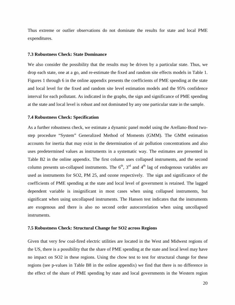
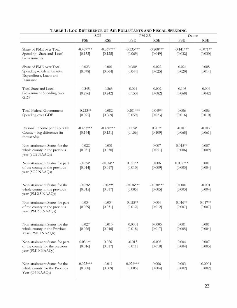
6. Results 6.1 Base Results

Table 1 presents the fixed and random site effects estimates for sulfur dioxide in columns 1 and

2, particulate matter in columns 3 and 4, and ozone in columns 5 and 6 respectively. The

Huber/White/Sandwich estimator of variance is used to estimate the standard errors to account

for heteroskedasticity. All estimates yield negative coefficients for the share of PME spending at

the state and local level of government, with a significance of at least 5%. The coefficients for

the share of PME spending at the state level range between -0.37 to -0.46 for SO2, -0.21 to -0.34

for PM 2.5, and -0.07 to -0.1 for O3. The share of PME spending at the state and local level of

7 Each type of spending is a combination of direct spending and assistance spending. Direct spending includes grants, salaries and wages, procurement contracts, and other direct payments. Direct assistance includes direct loans, guaranteed/insured loans and insurance (see Table A5). Assistance spending may also involve obligations indicated as negative amounts in CFFR. It is difficult to track, by program, when obligations were made, and how to distribute the negative amounts in prior years. Thus, negative figures are retained, and are included in the aggregate estimation of the spending type. 8 Administrative expenditures appear separately in the CFFR and have to be distributed. In some cases, all the programs in a department can be identified under one category of spending. When a whole department does not fall under one category of spending, the administrative expenditures are divided by the ratio of each type of spending over total department spending. In the case of pre-1993 data, the administrative spending is not allocated by department. Thus the administrative spending is first divided by the department by the proportion of department spending over total spending. This is then further divided into the type of spending, using the proportion of the type of spending over total department spending.

15

government is negative but largely insignificant. The total federal government spending effect is

not robust across pollutants; it has a negative and significant effect for PM 2.5, but loses

significance in the SO2 fixed site effects estimations. Furthermore the coefficient of total federal

spending switches to a positive sign and remains insignificant for the O3 estimations.9

The coefficient for personal income yields a negative coefficient significant at 1% for SO2. In

contrast the coefficient for personal income is insignificant for O3 but positive and marginally

significant at 10% for PM 2.5 air concentrations. One explanation may be that the personal

income variable captures both the scale and income effects. For production generated pollutants,

such as SO2, the income effect dominates, while for pollutants with a more significant

consumption source, such as O3 and PM 2.5, the scale effect dominates.

Both the partial and whole county non-attainment status variables for SO2 are negative, but only

the counties which partially had non-attainment status in the previous year results in a

statistically significant reduction in SO2, with a level of significance of 1%. The non-attainment

status for lead also has a significant negative effect on SO2 concentrations, which is expected

given that since the phasing out of lead from gasoline, industrial processes have been a major

contributor towards lead emissions. Both partial and whole PM2.5 non-attainment status in the

previous year has a highly significant (1% level) and negative effect on PM 2.5 air

concentrations. Also ozone non-attainment status for the whole county has a negative and

significant effect on PM 2.5 concentrations. In contrast, ozone non-attainment status has no

significant effect on ozone concentrations, however both partial and whole county non-

attainment status for the precursor pollutant – NO- has a negative effect on ozone concentrations

with significance of at least 5%. Partial non-attainment status of carbon monoxide (CO) also has

a significant and negative effect on ozone, which may not be surprising given that transportation

is a significant source of both CO and ozone emissions.

9 Some types of PME spending may take a large period of time to have an effect on environmental outcomes. We repeat the estimates in Table 1 using 3 year averages of the spending variable to capture the long term effects of the share of PME spending. The results in Table 1 are largely retained and are reported in table B6 in the online appendix. This implies that our results may be adequately capturing the affect of increasing the share of PME on the air pollutants.

16

One interesting result is that non-attainment status for certain pollutants may actually positively

contribute to increases in other pollutants. For instance partial and whole county non-attainment

status for CO has a marginally significant (mostly 10%) but positive effect on PM2.5

concentrations. Lead concentrations non-attainment status has a positive and significant effect on

PM 2.5 concentrations while partial county non-attainment status for PM 2.5 has a positive and

significant effect on ozone concentrations. This may imply that in attempt to address non-

attainment status for one pollutant, state governments may undertake activities that increase

other pollutants. This may mean there is a degree of substitutability in the regulation of

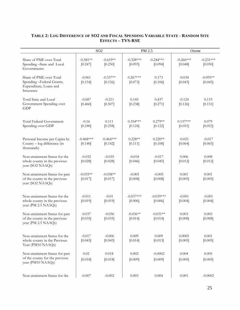
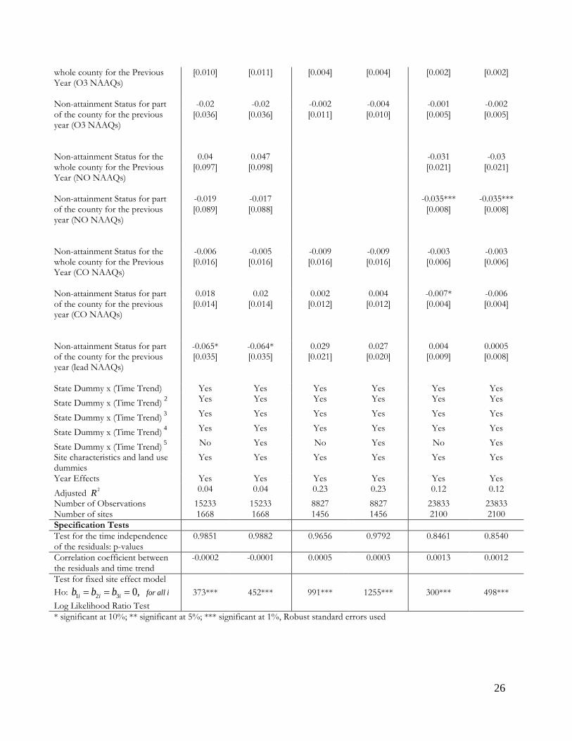
pollutants. 6.2 Time Varying State Effects (TVS) Results Table 2 presents the TVS-RSE model where we include both random site level effects and time

varying state level effects. Since the lowest number of observations per state is 6 for sulfur

dioxide and PM 2.5, we use the 4th polynomial to approximate stv 10. However, just to check for

consistency, we provide estimates including the 5th polynomial. Columns 1 and 2 of table 2 show

the 4th and 5th polynomial estimation results respectively for SO2. Similarly, columns 3 and 4 of

table 2 show the 4th and 5th polynomial estimation results for PM 2.5, while columns 5 and 6

show the 4th and 5th polynomial estimation results for ozone.

Using the 4th polynomial approximation of stv , the coefficient of the share of PME spending at

the state and local level retains the negative sign across all pollutants with a 5% level of

significance while federal PME spending remains insignificant. The size of the coefficient of the

share of PME spending at the state and local level is generally larger than OLS, random, and

fixed site effects coefficients reported in table 1. The sign and significance of personal income is

similar for all pollutants as in table 1, while total state and local government spending is

insignificant. Total federal spending has a positive and significant coefficient for PM 2.5, but is

otherwise insignificant for the SO2 and ozone. The non-attainment status variables do not

significantly differ from random and fixed estimations in table 1.

10 The low number of observations for some states is due to the fact that only monitoring sites with a consistent methodology in terms of length of time of the exposure are included in the study

17

The TVS-RSE residuals as indicated at the bottom of Table 2 are time independent11. The log

likelihood ratio test favors the TVS-RSE model over using state level fixed effects at the 1%

level of significance. We also estimated the TVS-FSE model as indicated in Table B1 in the

online appendix (see reference in footnote 1). Although the results are qualitatively similar to the

TVS-RSE model, the residuals are generally not time independent.

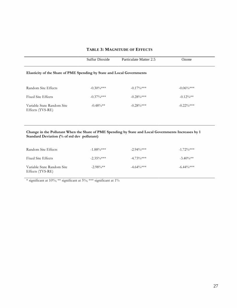
6.3 Magnitude of the Effects The elasticities of PME spending for state and local governments with respect to SO2, PM 2,5

and ozone concentrations are presented in columns 1,2 and 3 respectively in Table 3. Elasticities

using random site effects, fixed site effects, and TVS-RE are presented in rows 1, 2, and 3

respectively. Using the fixed and random site effects estimates in Table 1 and the TVS-RE (4th

polynomial) estimates in Table 3, a 10 % increase in the share of PME spending reduces sulfur

dioxide concentrations by 4%, 3%, and 5%, PM 2.5 by 3%, 2%, and 3%, and Ozone by 1%,

0.06%, and 2% respectively for state and local governments. The magnitude of all the effects

has a significance of at least 5%. The elasticities of 3 to 5% for the share of PME spending with

regards to SO2 concentrations are similar to the estimates in Lopez, Galinato and Islam (2011)

who find an elasticity of 3% using a panel 38 countries for the time period 1986 to 1999.

A one standard deviation increase in the share of PME spending by state and local governments

reduces SO2 concentrations by around 2 to 3%, depending on the type of estimation used. The

effect on PM2.5 concentrations is slightly larger with a one standard deviation increase in the

share of PME spending resulting in a 3 to 4% decline. The corresponding figures for Ozone

concentrations are between 2 to 6%. Results are presented in rows 4,5, and 6 of Table 3.

In almost all cases, the magnitude of the effects is larger for the TVS-RE estimations than the

fixed and random site effects. We interpret this result as possible evidence that the TVS-RE

estimations may be accounting for time varying omitted variables that weaken the effect of the

share of PME spending on the air pollutants as indicated by the smaller coefficient estimates of

11 The p-values presented at the bottom of table 3 test the time independence of the residual using the estimation constantjst trendε β= +

18

PME spending in the fixed and random site effects estimations vis-à-vis the TVS-RE

estimations.

7. Robustness We address a few additional concerns regarding our estimations. In additional to the TVS

estimation approach that accounts for time varying omitted variables that are difficult to

measure, we consider several other variables found in the literature to have a significant effect on

environmental outcomes and check whether they affect our results. Furthermore, outliers or

particular states may be driving our results. We also consider alternate specifications such as

GMM. Furthermore, given the distribution of power plants across the US, there may be structural

differences on the impact of PME spending on SO2. Finally, we address the issue of pollution

migration through spatial lag and spatial error model panel estimations.

7.1 Robustness Check: Added Controls Approach In addition to the TVS approach, we also address omitted variable bias using the added controls

approach. Studies have shown that several factors may directly or indirectly affect environmental

quality. Factors such as economic intensity (Antweiler et al., 2001; Grossman and Kruger, 1995;

Harbaugh et al., 2002), sector composition (Brooks and Sethi, 1997; Antweiler et al, 2001),

socioeconomic characteristics such as racial composition and economic conditions (Brooks and

Sethi, 1997; Khanna, 2002) have all been determinants of environmental quality. In addition,

pollution abatement costs may influence firms’ decisions to pollute and this may influence

environmental quality (Levinson , 1996; Levinson and Taylor, 2008). Since electric utilities

contribute significantly to SO2 and O3 emissions, total net generation of electricity may be an

important control variable for the base specification in equation (2). Price of natural gas or fuel,

fuel taxes, or the level of private capital may influence activities that generate emissions. Several

meteorological factors may also affect air quality such as wind speed and direction, temperature,

height of monitoring site probe, and elevation above sea level. Finally, pollution readings in a

state can be correlated by the no. of monitoring sites in the state. We add a set of variables

representing each of the determinants listed above in sequence into the random and fixed site

effect estimations in Table 1 to test the robustness of the variables of interest. Some of these

controls are interpolated due to sparse data. Pollution abatement costs data is linearly imputed for

19

the years 1987, 1995-1998, 2000-2004, and racial composition data from the census is linearly

imputed for the years 1981-1989, 1991-1999. The meteorological data is obtained from a few

sites that have the data, and assumed to be representative of the whole state.

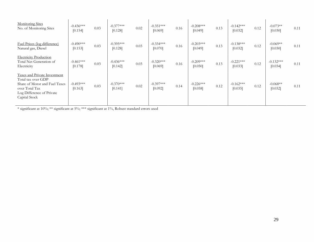
Table 4 shows the coefficients of the effect of PME spending for state and local governments as

each set of controls are added to the base estimations in Table 1. An increase in the adjusted R-

squared relative to the base estimations implies that including the additional sets of controls

raises the explanatory power of the model. If the coefficient of PME spending retains the sign

and significance, this implies that the coefficient is stable and robust to the additional regressors.

Table 4 shows that the coefficients of PME spending are largely unaffected by the additional sets

of control variables. Both the sign and significance of the PME spending coefficient is negative

and has a significance of at least 5%. The highly interpolated variables - racial composition

proxies and pollution abatement costs – raise the adjusted R squared across pollutants. Caution

should be employed in interpreting this as the degree of linear interpolation for these variables is

quite intensive. Meteorological conditions also raise the adjusted R squared for SO2 and ozone,

while not really altering the goodness of fit for PM 2.5. Considering the potential controls

presented in Table 4, we can conclude that the results are robust to omitted variables that are

correlated with these sets of variables. 7.2 Robustness Check: Extreme Observation Dominance A small number of outlier observations may be driving the results. In order to address this, we

drop the top 1%, the bottom 1%, and both top 1% and bottom 1% observations of the dependent

variable (log difference of air concentrations) and the variable of interest (PME spending for the

state and local government) and re-estimate the fixed and random state effects estimations in

Table 1 and the TVS-RSE estimations in Table 2 using the 4th polynomial. The results are

presented in Table B3, B4 and B5 in the online appendix for SO2, PM 2.5, and ozone

respectively. The signs of the coefficients for PME spending for the state and local levels of

government are negative and have at least a 10% level of significance for all the sample

alterations for random site effects and fixed site effects. This is also true for TVS-RSE estimates.

20

Thus extreme or outlier observations do not dominate the results for state and local PME

expenditures.

7.3 Robustness Check: State Dominance We also consider the possibility that the results may be driven by a particular state. Thus, we

drop each state, one at a go, and re-estimate the fixed and random site effects models in Table 1.

Figures 1 through 6 in the online appendix presents the coefficients of PME spending at the state

and local level for the fixed and random site level estimation models and the 95% confidence

interval for each pollutant. As indicated in the graphs, the sign and significance of PME spending

at the state and local level is robust and not dominated by any one particular state in the sample.

7.4 Robustness Check: Specification As a further robustness check, we estimate a dynamic panel model using the Arellano-Bond two-

step procedure “System” Generalized Method of Moments (GMM). The GMM estimation

accounts for inertia that may exist in the determination of air pollution concentrations and also

uses predetermined values as instruments in a systematic way. The estimates are presented in

Table B2 in the online appendix. The first column uses collapsed instruments, and the second

column presents un-collapsed instruments. The 6th, 3rd and 4th lag of endogenous variables are

used as instruments for SO2, PM 25, and ozone respectively. The sign and significance of the

coefficients of PME spending at the state and local level of government is retained. The lagged

dependent variable is insignificant in most cases when using collapsed instruments, but

significant when using uncollapsed instruments. The Hansen test indicates that the instruments

are exogenous and there is also no second order autocorrelation when using uncollapsed

instruments. 7.5 Robustness Check: Structural Change for SO2 across Regions

Given that very few coal-fired electric utilities are located in the West and Midwest regions of

the US, there is a possibility that the share of PME spending at the state and local level may have

no impact on SO2 in these regions. Using the chow test to test for structural change for these

regions (see p-values in Table B8 in the online appendix) we find that there is no difference in

the effect of the share of PME spending by state and local governments in the Western region

21

from the base estimations. However at the 10% level of significance, we reject that the Midwest

region has parameter estimates equal to the base regressions. Re-estimations of the RE and FE

models for the Midwest region alone retains the sign and significance of the share of PME

spending for state and local governments. We present the p-values of the chow test in table B8

and the classification of regions in table B9 in the online appendix. 7.6 Robustness Check: Pollution Migration Monitoring sites near the border of states may pick up air pollution concentrations originating

from neighboring states. Similarly monitoring sites in a state may read low levels of air pollution

concentrations as they are blown away to other states. This invites the possibility of spurious

correlation. We account for this by estimating spatial lag and error panel models. For these

estimations we create a county-level panel dataset, by averaging the pollution concentrations

over all the monitoring sites in a county. We only retain counties that have data for the full time

period. For the spatial estimations we use a row standardized inverse distance weighting matrix

of the 5 nearest counties. The results of the spatial lag and spatial error random effects models

are presented separately for each pollutant in Table A7. The maps in figures 7 through 9 in the

online appendix show the counties in the sample and the spatial relations between them. The

results in Table A7 indicate that the share of PME spending for the state and local level has a

negative coefficient and retains significance of about 5% for all pollutants. Both the spatial lag

and spatial autocorrelation terms are significant at 1%. This implies that although the spatial

aspect of the pollutants is important, the negative effect of the share of PME spending for state

and local governments on SO2, O3, and PM2.5 is robust to it.

8. Conclusion This paper examines the effect of government spending at various levels of government on air

pollution in the US. We find that the size of the public sector is not important but what matters is

the composition of spending at the state and local level of government. A reallocation of

government spending from private subsidies to social and public good spending that alleviates

market failures and increases public goods, holding total government spending fixed, results in

significant reductions in SO2, PM 2.5, and O3 concentrations for state and local governments but

not the federal government. After subjecting the results to rigorous tests that limit the effect of

22

omitted variable bias, consider sensitivity towards sample alterations, and account for spatial

issues, we find that the effect of state and local PME spending is robust. The results are

consistent with the findings of Lopez, Galinato and Islam (2011) who find a negative effect of a

reallocation from RME to PME spending on air and water pollutants.

In the light of the present economic circumstances, this study is a timely addition to the debate

on US government spending priorities. While the effect of total government spending on

pollution appears to be neutral, the reductions of sulfur dioxide air pollution by increasing the

share PME spending at the local level may imply that reductions in US state government

spending under huge budget deficits should be taken with care. Even though the main goal of

fiscal policy is not to alleviate environmental concerns, it is important to consider the effects they

may have on the environment, potentially affecting the impact of existing and potentially costly

environmental regulations.

23

TABLE 1: LOG DIFFERENCE OF AIR POLLUTANTS AND FISCAL SPENDING SO2 PM 2.5 Ozone FSE RSE FSE RSE FSE RSE Share of PME over Total Spending –State and Local Governments

-0.457***

-0.367***

-0.335***

-0.208***

-0.141***

-0.071**

[0.153] [0.128] [0.069] [0.049] [0.032] [0.030]

Share of PME over Total Spending –Federal Grants, Expenditure, Loans and Insurance

-0.023 -0.001 0.080* -0.022 -0.024 0.005 [0.078] [0.064] [0.044] [0.025] [0.020] [0.014]

Total State and Local Government Spending over GDP

-0.345 -0.363 -0.094 -0.002 -0.103 -0.004 [0.296] [0.242] [0.153] [0.082] [0.068] [0.042]

Total Federal Government Spending over GDP

-0.223** -0.082 -0.201*** -0.049** 0.006 0.006 [0.095] [0.069] [0.059] [0.023] [0.016] [0.010]

Personal Income per Capita by County – log difference (in thousands)

-0.453*** -0.438*** 0.274* 0.207* -0.018 -0.017 [0.144] [0.131] [0.156] [0.109] [0.068] [0.061]

Non-attainment Status for the whole county in the previous year (SO2 NAAQs)

-0.022 -0.031 0.007 0.015** 0.007 [0.031] [0.030] [0.051] [0.006] [0.009]

Non-attainment Status for part of the county in the previous year (SO2 NAAQs)

-0.024* -0.034** 0.021** 0.006 0.007*** 0.001 [0.014] [0.017] [0.010] [0.009] [0.003] [0.004]

Non-attainment Status for the whole county in the previous year (PM 2.5 NAAQs)

-0.026* -0.029* -0.036*** -0.038*** 0.0001 -0.001 [0.015] [0.017] [0.005] [0.005] [0.003] [0.004]

Non-attainment Status for part of the county in the previous year (PM 2.5 NAAQs)

-0.034 -0.034 0.025** 0.004 0.016** 0.017** [0.029] [0.031] [0.012] [0.012] [0.007] [0.007]

Non-attainment Status for the whole county in the Previous Year (PM10 NAAQs)

-0.027 -0.013 -0.0001 0.0005 0.001 0.001 [0.026] [0.046] [0.018] [0.017] [0.005] [0.004]

Non-attainment Status for part of the county for the previous year (PM10 NAAQs)

0.036** 0.026 -0.013 -0.008 0.004 0.007 [0.016] [0.017] [0.011] [0.010] [0.004] [0.005]

Non-attainment Status for the whole county for the Previous Year (O3 NAAQs)

-0.023*** -0.011 0.026*** 0.006 0.003 -0.0004 [0.008] [0.009] [0.005] [0.004] [0.002] [0.002]

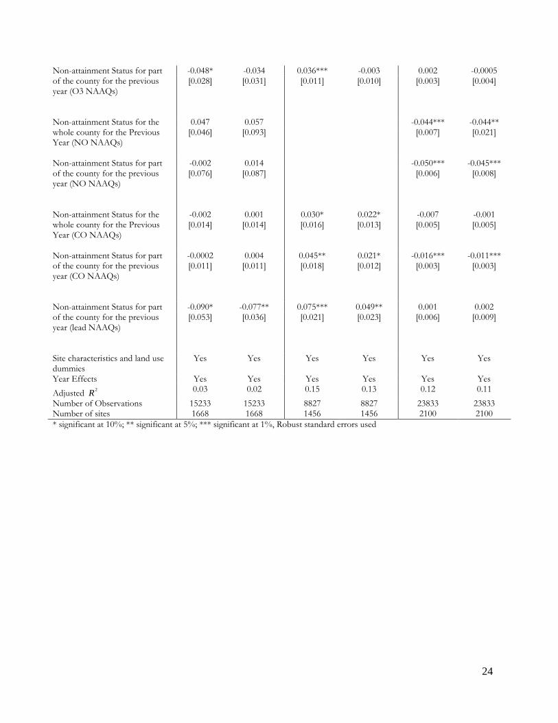
24

Non-attainment Status for part of the county for the previous year (O3 NAAQs)

-0.048* -0.034 0.036*** -0.003 0.002 -0.0005 [0.028] [0.031] [0.011] [0.010] [0.003] [0.004]

Non-attainment Status for the whole county for the Previous Year (NO NAAQs)

0.047 0.057 -0.044*** -0.044** [0.046] [0.093] [0.007] [0.021]

Non-attainment Status for part of the county for the previous year (NO NAAQs)

-0.002 0.014 -0.050*** -0.045*** [0.076] [0.087] [0.006] [0.008]

Non-attainment Status for the whole county for the Previous Year (CO NAAQs)

-0.002 0.001 0.030* 0.022* -0.007 -0.001 [0.014] [0.014] [0.016] [0.013] [0.005] [0.005]

Non-attainment Status for part of the county for the previous year (CO NAAQs)

-0.0002 0.004 0.045** 0.021* -0.016*** -0.011*** [0.011] [0.011] [0.018] [0.012] [0.003] [0.003]

Non-attainment Status for part of the county for the previous year (lead NAAQs)

-0.090* -0.077** 0.075*** 0.049** 0.001 0.002 [0.053] [0.036] [0.021] [0.023] [0.006] [0.009]

Site characteristics and land use dummies

Yes Yes Yes Yes Yes Yes

Year Effects Yes Yes Yes Yes Yes Yes Adjusted 2R 0.03 0.02 0.15 0.13 0.12 0.11

Number of Observations 15233 15233 8827 8827 23833 23833 Number of sites 1668 1668 1456 1456 2100 2100 * significant at 10%; ** significant at 5%; *** significant at 1%, Robust standard errors used

25

TABLE 2: LOG DIFFERENCE OF SO2 AND FISCAL SPENDING VARIABLE STATE - RANDOM SITE

EFFECTS – TVS-RSE

SO2 PM 2.5 Ozone Share of PME over Total Spending –State and Local Governments

-0.581**

-0.619**

-0.328***

-0.244***

-0.266***

-0.231***

[0.247] [0.250] [0.093] [0.094] [0.048] [0.050]


-0.061 -0.337** 0.267*** 0.173 -0.034 -0.095** [0.154] [0.156] [0.073] [0.106] [0.043] [0.045]


-0.687 -0.211 0.145 0.437 -0.124 0.119 [0.460] [0.507] [0.238] [0.271] [0.126] [0.151]


-0.16 0.111 0.354*** 0.279** 0.137*** 0.079 [0.240] [0.258] [0.124] [0.122] [0.051] [0.052]


-0.468*** -0.464*** 0.228** 0.220** -0.021 -0.017 [0.140] [0.142] [0.111] [0.108] [0.064] [0.065]


-0.032 -0.035 -0.018 -0.017 0.006 0.008 [0.028] [0.028] [0.046] [0.045] [0.012] [0.012]


-0.035** -0.038** -0.005 -0.005 0.001 0.001 [0.017] [0.017] [0.008] [0.008] [0.005] [0.005]


-0.011 -0.01 -0.037*** -0.039*** -0.001 -0.001 [0.019] [0.019] [0.006] [0.006] [0.004] [0.004]


-0.037 -0.036 -0.036** -0.031** 0.003 0.003 [0.035] [0.035] [0.014] [0.014] [0.008] [0.008]


-0.017 -0.006 0.009 0.009 0.0005 0.001 [0.043] [0.043] [0.014] [0.013] [0.005] [0.005]


0.02 0.018 0.002 -0.0002 0.004 0.005 [0.018] [0.018] [0.009] [0.009] [0.005] [0.005]

Non-attainment Status for the -0.007 -0.002 0.003 0.004 0.001 -0.0002

26

whole county for the Previous Year (O3 NAAQs)

[0.010] [0.011] [0.004] [0.004] [0.002] [0.002]


-0.02 -0.02 -0.002 -0.004 -0.001 -0.002 [0.036] [0.036] [0.011] [0.010] [0.005] [0.005]


0.04 0.047 -0.031 -0.03 [0.097] [0.098] [0.021] [0.021]


-0.019 -0.017 -0.035*** -0.035*** [0.089] [0.088] [0.008] [0.008]


-0.006 -0.005 -0.009 -0.009 -0.003 -0.003 [0.016] [0.016] [0.016] [0.016] [0.006] [0.006]


0.018 0.02 0.002 0.004 -0.007* -0.006 [0.014] [0.014] [0.012] [0.012] [0.004] [0.004]


-0.065* -0.064* 0.029 0.027 0.004 0.0005 [0.035] [0.035] [0.021] [0.020] [0.009] [0.008]

State Dummy x (Time Trend) Yes Yes Yes Yes Yes Yes State Dummy x (Time Trend) 2 Yes Yes Yes Yes Yes Yes

State Dummy x (Time Trend) 3 Yes Yes Yes Yes Yes Yes

State Dummy x (Time Trend) 4 Yes Yes Yes Yes Yes Yes

State Dummy x (Time Trend) 5 No Yes No Yes No Yes Site characteristics and land use dummies

Yes Yes Yes Yes Yes Yes

Year Effects Yes Yes Yes Yes Yes Yes

Adjusted 2R 0.04 0.04 0.23 0.23 0.12 0.12 Number of Observations 15233 15233 8827 8827 23833 23833 Number of sites 1668 1668 1456 1456 2100 2100 Specification Tests Test for the time independence of the residuals: p-values

0.9851 0.9882 0.9656 0.9792 0.8461 0.8540

Correlation coefficient between the residuals and time trend

-0.0002 -0.0001 0.0005 0.0003 0.0013 0.0012

Test for fixed site effect model Ho: 1 2 3 0,i i i for all ib b b= = = Log Likelihood Ratio Test

373*** 452*** 991*** 1255*** 300*** 498***

* significant at 10%; ** significant at 5%; *** significant at 1%, Robust standard errors used

27

TABLE 3: MAGNITUDE OF EFFECTS

Sulfur Dioxide Particulate Matter 2.5 Ozone

Elasticity of the Share of PME Spending by State and Local Governments

Random Site Effects

-0.30%*** -0.17%*** -0.06%***

Fixed Site Effects

-0.37%*** -0.28%*** -0.12%**

Variable State Random Site Effects (TVS-RE)

-0.48%** -0.28%*** -0.22%***

Change in the Pollutant When the Share of PME Spending by State and Local Governments Increases by 1 Standard Deviation (% of std dev pollutant)

Random Site Effects

-1.88%*** -2.94%*** -1.72%***

Fixed Site Effects

-2.35%*** -4.73%*** -3.40%**

Variable State Random Site Effects (TVS-RE)

-2.98%** -4.64%*** -6.44%***

* significant at 10%; ** significant at 5%; *** significant at 1%

28

TABLE 4: ADDED CONTROLS APPROACH – STATE AND LOCAL SHARE OF PME

SO2 PM 2.5 Ozone

FSE RSE FSE RSE FSE RSE Coef. Adjusted

R squared

Coef. Adjusted R squared



Coef. Adjusted R

squared

Coef. Adjusted R

squared

Base

-0.457***

0.03

-0.367***

0.02

-0.335***

0.15

-0.208***

0.13

-0.141***

0.12

-0.071**

0.11

[0.153] [0.128] [0.069] [0.049] [0.032] [0.030] Economic Intensity GDP per Land (sq km), GDP growth, Population Density

-0.471***

[0.154] 0.03

-0.371***

[0.128] 0.02 -0.331***

[0.071] 0.15 -0.208*** [0.050] 0.13 -0.135***

[0.032] 0.l2 -0.068** [0.030] 0.11

Sector Composition Share of Manufacturing over GDP Employment in Manufacturing

-0.457*** [0.156] 0.03 -0.359***

[0.129] 0.02 -0.276*** [0.071] 0.16 -0.228***

[0.049] 0.13 -0.137*** [0.032] 0.12 -0.069**

[0.031] 0.11

Economic Conditions Unemployment Rate Poverty Rate

-0.456*** [0.154] 0.03 -0.357***

[0.128] 0.02 -0.338*** [0.069] 0.16 -0.181***

[0.051] 0.13 -0.145*** [0.032] 0.12 -0.067**

[0.031] 0.11

Pollution Abatement Costs & Racial Composition Capital Costs lagged Operating Costs lagged % white, % black

-0.377** [0.179] 0.04 -0.414***

[0.147] 0.04 -0.357*** [0.080] 0.17 -0.257***

[0.060] 0.15 -0.233*** [0.034] 0.16 -0.088***

[0.028] 0.16

Wind Speed and Direction Average Wind Speed, Wind Direction

-0.314** [0.155] 0.03 -0.258*

[0.133] 0.02 -0.381*** [0.070] 0.17 -0.169***

[0.052] 0.15 -0.128*** [0.035] 0.14 -0.074**

[0.029] 0.14

Temperature and Geographical Conditions Temperature, Elevation Above Sea Level, Height of Monitoring Site Probe

-0.487*** [0.175] 0.04 -0.331**

[0.155] 0.03 -0.322*** [0.080] 0.15 -0.191***

[0.053] 0.13 -0.204*** [0.035] 0.14 -0.094***

[0.035] 0.14

29

Monitoring Sites No. of Monitoring Sites

-0.436*** [0.154] 0.03 -0.377***

[0.128] 0.02 -0.351*** [0.069] 0.16 -0.208***

[0.049] 0.13 -0.142*** [0.032] 0.12 -0.073**

[0.030] 0.11

Fuel Prices (log difference) Natural gas, Diesel

-0.490*** [0.153] 0.03 -0.395***

[0.128] 0.03 -0.334*** [0.070] 0.16 -0.203***

[0.049] 0.13 -0.138*** [0.032] 0.12 -0.069**

[0.030] 0.11

Electricity Production Total Net Generation of Electricity

-0.461*** [0.178] 0.03 -0.436***

[0.142] 0.03 -0.320*** [0.069] 0.16 -0.209***

[0.050] 0.13 -0.221*** [0.033] 0.12 -0.132***

[0.034] 0.11

Taxes and Private Investment Total tax over GDP Share of Motor and Fuel Taxes over Total Tax Log Difference of Private Capital Stock

-0.493*** [0.163] 0.03 -0.370***

[0.141] 0.02 -0.397*** [0.092] 0.14 -0.226***

[0.058] 0.12 -0.162*** [0.035] 0.12 -0.068**

[0.032] 0.11

* significant at 10%; ** significant at 5%; *** significant at 1%, Robust standard errors used

30

References

Adeyemi, O. I., and L.C. Hunt (2007), "Modelling OECD Industrial Energy Demand: Asymmetric Price Responses and Energy-Saving Technical Change," Energy Economics 29(2007): 693-709

Altonji, J. G., T. E. Elder, and C. R. Taber (2005) “Selection on Observed and Unobserved variables: Assessing the Effectiveness of Catholic Schools.” Journal of Political Economy 113(1), 151—184.

Antweiler, W., B. R. Copeland, and M. S. Taylor (2001), “Is Free Trade Good for the Environment?” American Economic Review, 91 (4) 877-908.

Attanasio, O. P., P. K. Goldberg, and E. Kyriazidou (2008), “Credit Constraints in the Market for Consumer Durables: Evidence from Micro Data on Car Loans.” International Economic Review, 49(2): 401-436.

Auffhammer, M., A. M. Bento, S. E. Lowe (2011), “The City-Level Effects of the 1990 Clean Air Act Amendments.” Land Economics, 87(1), 1-18. Auffhammer, M., A. M. Bento, S. E. Lowe (2009), “Measuring the Effects of the Clean Air Act Amendments on Ambient PM10 Concentrations: The Critical Importance of a Spatially Disaggregated Analysis.” Journal of Environmental Economics and Management, 58(1), 15-26. Bai, J. (2009), "Panel Data Models With Interactive Fixed Effects." Econometrica 77(4): 1229-1279. Barrett, S., and K. Graddy (2000), “Freedom, Growth, and the Environment.” Environment and Development Economics 5: 433-456.

Bergman, L. (2005), "CGE modeling of environmental policy and resource management." In Handbook of Environmental Economics, ed. K-G Maler and Jeffrey Vincent, Vol. 3., Chapter 24. New York, NY: North-Holland, pp. 1273–1306. Bernauer, T. and V. Koubi (2006), "States as Providers of Public Goods: How Does Government Size Affect Environmental Quality?" Available at SSRN: http://ssrn.com/abstract=900487

Brooks, N. and R. Sethi (1997), “The Distribution of Pollution: Community Characteristics and Exposure to Air Toxics.” Journal of Environmental Economics and Management 32: 233-350 Carlson, C., D. Burtraw, M. Cropper, and K. L. Palmer (2000), “Sulfur Dioxide Control by Electric Utilities: What Are the Gaines from Trade?” The Journal of Political Economy 108: 1292-1326 Coady, D., M. E. Said, R. Gillingham, K. Kpoda, P. Medas, D. Newhouse (2006), “The Magnitude and Distribution of Fuel Subsidies: Evidence from Bolivia, Ghana, Jordan, Mali, and Sri Lanka.” IMF Working Paper 06/247.

http://ssrn.com/abstract=900487

31

Cebula, R. J., and N. Herder (2010), “An Empirical Analysis of Determinants of Commercial and Industrial Electricity Consumption.” Business and Economics Journal 2010: BEJ-7

Cornwell, C., P. Schmidt, and R. C. Sickles (1990), "Production Frontiers With Cross-Sectional and Time-Series Variation in Efficiency Levels." Journal of Econometrics 46 (1990): 185-200.

Curry, T., Shibut, L. (2000), “The Cost of the Savings and Loan Crisis: Truth and Consequences.” FDIC Banking Review.

Dasgupta, P. (1996), “The Economics of the environment.” Environment and Development Economics 1 (4): 378-428.

David, P. A., B. H. Hall, A. A. Toole (2000), “Is Public R&D a Complement or Substitute for Private R&D.” Research Policy 29(2000): 497-529.

Deacon, R. T. and C. Norman (2007), “Is The Environmental Kuznets Curve an Empirical Regularity?” In R. Halvorsen and D. Layton, Frontiers of Environmental and Natural Resource Economics, Edward Elgar Publishers, U.K.

Ferrer-i-Carbonell, A. and J.C.J.M. van den Bergh (2004), "A Micro-Econometric Analysis of Determinants of Unsustainable Consumption in the Netherlands." Environmental & Resource Economics 27(4): 367-389.

Filippini, M., and L. C. Hunt (2011), "Energy Demand and Energy Efficiency in the OECD Countries: A Stochastic Demand Frontier Approach," The Energy Journal 32(2): 59-80

Friedberg, L. (1998), "Did Unilateral Divorce Raise Divorce Rates? Evidence from Panel Data." American Economic Review 88(3): 608-627. Frankel J A, Rose A K (2005) Is Trade Good or Bad for the Environment: Sorting Out the Causality. Review of Economics and Statistics 87:85–91

Galor, O. and J. Zeira (1993), “Income Distribution and Macroeconomics.” Review of Economic Studies 60: 35-52.

Gerking, S., S. F. Hamilton (2010), “SO2 Policy and Input Substitution Under Spatial Monopoly.” Resource and Energy Economics 32(2010) 327-340. Grant, C. (2007), “Estimating Credit Constraints Among US households.” Oxford Economic Papers 59(4): 583-605.

Greenstone, M. (2004), “Did the Clean Air Act Cause the Remarkable Decline in Sulfur Dioxide Concentrations?” Journal of Environmental Economics and Management, 47(3): 5850611.

32

Grossman, G. M., and A. B. Krueger (1995), “Economic Growth and the Environment.” Quarterly Journal of Economics, 112 (2) 353-378.

Harbaugh, W., A. Levinson, and D. Wilson (2002), “Reexamining the Empirical Evidence for an Environmental Kuznets Curve.” Review of Economics and Statistics, 84(3): 541-551

Henderson, J. V. (1996), “Effects of Air Quality Regulation.” American Economic Review, 86(4), 789-813.

Hoff, K., and J. E. Stiglitz (2000). “Modern Economic Theory and Development.” In: Meier, G., Stiglitz, J. (Eds.), Frontiers of Development Economics. Oxford University Press and the World Bank, New York.

Islam , A. (2011), “US Government Spending Allocation Database by State,” draft paper, University of Maryland, College Park (Dissertation Chapter).

Jacobsen L. S., R. J. Lalonde, and D. G. Sullivan (1993), "Earnings Losses of Displaced Workers." American Economic Review 83(4): 685-709.

Jappelli, T. (1990), “Who is Credit Constrained in the US Economy?” Quarterly Journal of Economics 105(1): 219-234

Jorgenson, D.W. and P. Wilcoxen (1990), “Intertemporal General Equilibrium Modeling of U.S. Environmental Regulation”, Journal of Policy Modeling, 12(4):715-744.

Kamerschen, D. R., and D.V. Porter (2004), "The Demand for Residential, Industrial, and Total Electricity, 1973-1998" Energy Economics 26 (2004): 87-100

Kamerschen, D. R., P. G. Klein, and D. V. Porter (2005) "Market Structure in the US Electricity Industry: A Long-Term Perspective" Energy Economics 27 (2005): 731-751

Khanna, N. (2001) "Analyzing the Economic Cost of the Kotyo Protocol," Ecological Economics 38(2001): 59-69

Khanna, N. (2002), "Is Air Quality Income Elastic? Revisiting the Environmental Kuznets Curve Hypothesis," working paper WP0207, Department of Economics, Binghampton University, Binghampton NY.

Kim, D., and T. Oka (2012), “Divorce Law Reforms and Divorce Rates in the U.S.: An Interactive Fixed Effects Approach” forthcoming, Journal of Applied Econometrics Kneip, A., R. C. Sickles, and W. Song (2011), “A New Panel Data Treatment for Heterogeneity in Time Trends,” forthcoming in Econometric Theory, 2011.

33

Kummel, R., J. Schmid,R. U. Ayers, and D. Lindenberger (2008), "Cost Shares, Output Elasticities, and Substitutability Constraints," EWI Working Paper, No 08.02.

Levinson, A. (1996), "Environmental regulations and manufacturers' location choices: Evidence from the Census of Manufactures," Journal of Public Economics 62: 5-29.

Levinson, A. and M. S. Taylor (2008), “Unmasking the Pollution Haven Effect,” International Economic Review 49(1):223-254.

List, J. A. and C. A. Gallet, (1999), “The Environmental Kuznets Curve: Does One Size Fit All?” Ecological Economics 31: 409-423.

Liu, G. (2004), "Estimating Energy Demand Elasticities for OECD Countries: A Dynamic Panel Data Approach," Statistics Norway Research Department, Discussion Papes No. 373.

López, R, and G. Galinato, (2007). Should Governments Stop Subsidies to Private Goods? Evidence from Rural Latin America. Journal of Public Economics 91, 1071-1094. López, R., and G. Galinato and A. Islam (2011), “Fiscal Spending and the Environment: Theory and Empirics.” Journal of Environmental Economics and Management, 62: 180-198.

López, R., and A. Islam (2011). “Fiscal spending for economic growth in the presence of imperfect Markets.” CEPR Discussion Paper no. 8709. London, Centre for Economic Policy Research. http://www.cepr.org/pubs/dps/DP8709.asp

López, R., and A. Palacios (2011), “Why Europe Has Become Environmentally Cleaner: Decomposing the Roles of Fiscal, Trade and Environmental Policies” CEPR Discussion Paper no. 8551. London, Centre for Economic Policy Research. http://www.cepr.org/pubs/dps/DP8551.asp

McConnell, Kenneth E. (1997), "Income and the Demand for Environmental Quality" Environment and Development Economics 2(1997): 383-399 McAusland, C. (2008), “Trade, Politics, and the Environment: Tailpipe vs. Smokestack” Journal of Environmental Economics and Management 55(1): 52-71.

Oates, W. E. (1999), “An Essay on Fiscal Federalism.” Journal of Economic Literature, 37(3):1120-1149

Oates, W. E. (2001), “A Reconsideration of Environmental Federalism.” University of Maryland, College Park. Unpublished paper. Olund, K. (2010) "The Industrial Electricity Use in the OECD Countries," Lulea University of Technology thesis, 2010

http://www.cepr.org/pubs/dps/DP8709.asp

http://www.cepr.org/pubs/dps/DP8551.asp

34

Orecchia, C. and M. E. Tessitore (2011), "Economic Growth and the Environment with Clean and Dirty Consumption." FEEM Working Paper No. 57.2011. Available at SSRN:http://ssrn.com/abstract=1915838 Selden, T.M. and D. Song (1995), “Neoclassical growth, the j curve for abatement and the inverted u curve for pollution” Journal of Environmental Economics and Management 29: 162–168.

Shafik, N., and S. Bandyopadhyay (1992), “Economic Growth and Environmental Quality: Time Series and Cross-country evidence.” background paper for World Development Report 1992, World Bank, Washington, DC, June.

Shapiro R.J., K.A Hassett, F. S. Arnold (2002), “Conserving Energy and Preserving the Environment: The Role of Public Transportation.” Washington, DC: APTA; 2002:2. Available at: http://www.apta.com/research/info/online/shapiro.cfm. Accessed November 11, 2004.

Slivinski, S. (2007), “The Corporate Welfare State - How the Federal Government Subsidizes US businesses.” Working Paper Policy Analysis No. 592, CATO Institute, May Stresing, R., D. Lindenberger, and R.Kummel (2008), "Cointegration of output, cappital, labor, and energy," The European Physical Journal B - Condensed Matter and Complex Systems 88(2): 279-287. U.S. Environmental Protection Agency (EPA) (2003), National Air Pollutant Emission Trends, 2003, Report EPA-454/R-03-005, EPA, Office of Air Quality and Standards, Air Quality Strategies and Standards Division Research Triangle Park, NC.

Wolfers, J. (2006), "Did Unilateral Divorce Laws Raise Divorce Rates? A Reconciliation and New Results." American Economic Review 96(5): 1802-1820.

Yamarik, S. (2011), “State-Level Capital and Investment: Updates and Implications.” Contemporary Economic Policy http://dx.doi.org/10.1111/j.1465-7287.2011.00282.x

Zeldes, S. P. (1989), “Consumption and Liquidity Constraints: An Empirical Analysis.” Journal of Political Economy 97(2): 305-346

Zimmerman, Rae (2005), "Mass Transit Infrastructure and Urban Health" Journal of Urban Health 82(1): 21-32

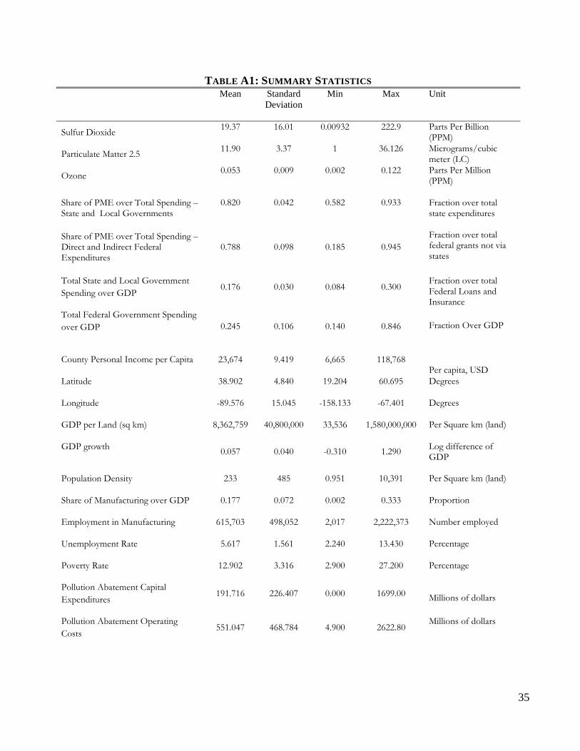
http://dx.doi.org/10.1111/j.1465-7287.2011.00282.x

35

TABLE A1: SUMMARY STATISTICS

Mean Standard Deviation

Min Max Unit

Sulfur Dioxide 19.37 16.01 0.00932 222.9 Parts Per Billion (PPM)

Particulate Matter 2.5 11.90 3.37 1 36.126 Micrograms/cubic meter (LC)

Ozone 0.053 0.009 0.002 0.122 Parts Per Million (PPM)

Share of PME over Total Spending –State and Local Governments

0.820 0.042 0.582 0.933 Fraction over total state expenditures

Share of PME over Total Spending – Direct and Indirect Federal Expenditures

0.788 0.098 0.185 0.945 Fraction over total federal grants not via states


0.176 0.030 0.084 0.300 Fraction over total Federal Loans and Insurance


0.245 0.106 0.140 0.846 Fraction Over GDP

County Personal Income per Capita

23,674 9.419 6,665 118,768 Per capita, USD

Latitude 38.902 4.840 19.204 60.695 Degrees

Longitude -89.576 15.045 -158.133 -67.401 Degrees

GDP per Land (sq km) 8,362,759 40,800,000 33,536 1,580,000,000 Per Square km (land)

GDP growth 0.057 0.040 -0.310 1.290 Log difference of GDP

Population Density 233 485 0.951 10,391 Per Square km (land)

Share of Manufacturing over GDP 0.177 0.072 0.002 0.333 Proportion

Employment in Manufacturing 615,703 498,052 2,017 2,222,373 Number employed

Unemployment Rate 5.617 1.561 2.240 13.430 Percentage

Poverty Rate 12.902 3.316 2.900 27.200 Percentage

Pollution Abatement Capital Expenditures

191.716 226.407 0.000 1699.00 Millions of dollars

Pollution Abatement Operating Costs

551.047 468.784 4.900 2622.80 Millions of dollars

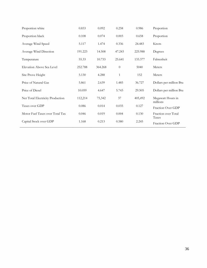
36

Proportion white 0.833 0.092 0.258 0.986 Proportion

Proportion black 0.108 0.074 0.003 0.658 Proportion

Average Wind Speed 5.117 1.474 0.336 24.483 Knots

Average Wind Direction 191.223 14.508 47.243 225.988 Degrees

Temperature 55.33 10.733 25.641 133.377 Fahrenheit

Elevation Above Sea Level 252.788 364.268 0 5040 Meters

Site Prove Height 5.130 4.288 1 152 Meters

Price of Natural Gas 5.861 2.639 1.485 36.727 Dollars per million Btu

Price of Diesel 10.059 4.647 5.743 29.505 Dollars per million Btu

Net Total Electricity Production 112,214 75,342 37 405,492 Megawatt Hours in millions

Taxes over GDP 0.086 0.014 0.035 0.127 Fraction Over GDP

Motor Fuel Taxes over Total Tax 0.046 0.019 0.004 0.130 Fraction over Total Taxes

Capital Stock over GDP 1.168 0.213 0.580 2.245 Fraction Over GDP

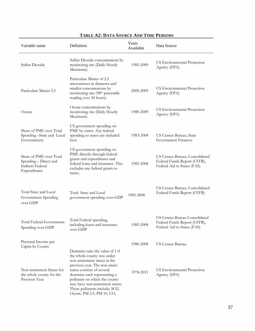
37

TABLE A2: DATA SOURCE AND TIME PERIODS Variable name

Definition Years Available Data Source

Sulfur Dioxide

Sulfur Dioxide concentrations by monitoring site (Daily Hourly Maximum)

1985-2009 US Environmental Protection Agency (EPA)

Particulate Matter 2.5

Particulate Matter of 2.5 micrometers in diameter and smaller concentrations by monitoring site (98th percentile reading over 24 hours)


Ozone Ozone concentrations by monitoring site (Daily Hourly Maximum)



US government spending on PME by states. Any federal spending to states are included here

1983-2008 US Census Bureau, State Government Finances

Share of PME over Total Spending – Direct and Indirect Federal Expenditures

US government spending on PME directly through federal grants and expenditures and federal loans and insurance. This excludes any federal grants to states.

1983-2008

US Census Bureau, Consolidated Federal Funds Report (CFFR), Federal Aid to States (FAS)


Total State and Local government spending over GDP 1983-2008

US Census Bureau, Consolidated Federal Funds Report (CFFR)


Total Federal spending, including loans and insurance over GDP

1983-2008

US Census Bureau Consolidated Federal Funds Report (CFFR), Federal Aid to States (FAS)

Personal Income per Capita by County 1980-2008 US Census Bureau

Non-attainment Status for the whole county for the Previous Year

Dummies take the value of 1 if the whole county was under non-attainment status in the previous year. The non-attain status consists of several dummies each representing a pollutant on which the county may have non-attainment status. These pollutants include: SO2, Ozone, PM 2.5, PM 10, CO,


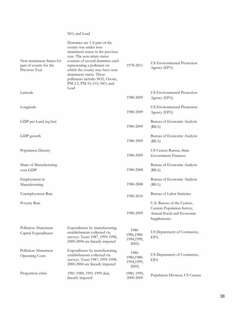
38

NO, and Lead

Non-attainment Status for part of county for the Previous Year

Dummies are 1 if part of the county was under non-attainment status in the previous year. The non-attain status consists of several dummies each representing a pollutant on which the county may have non-attainment status. These pollutants include: SO2, Ozone, PM 2.5, PM 10, CO, NO, and Lead


Latitude 1980-2009

US Environmental Protection Agency (EPA)

Longitude 1980-2009

US Environmental Protection Agency (EPA)

GDP per Land (sq km) 1980-2009

Bureau of Economic Analysis (BEA)

GDP growth 1980-2009


Population Density 1980-2009

US Census Bureau, State Government Finances

Share of Manufacturing over GDP 1980-2008


Employment in Manufacturing 1980-2008


Unemployment Rate 1980-2010 Bureau of Labor Statistics

Poverty Rate

1980-2009

U.S. Bureau of the Census, Current Population Survey, Annual Social and Economic Supplements

Pollution Abatement Capital Expenditures

Expenditures by manufacturing establishments collected via surveys. Years 1987, 1995-1998, 2000-2004 are linearly imputed

1980-1986,1988-1994,1999,

2005)

US Department of Commerce, EPA

Pollution Abatement Operating Costs

Expenditures by manufacturing establishments collected via surveys. Years 1987, 1995-1998, 2000-2004 are linearly imputed

1980-1986,1988-1994,1999,

2005)

US Department of Commerce, EPA

Proportion white 1981-1989, 1991-1999 data linearly imputed

1980, 1990, 2000-2009

Population Division, US Census

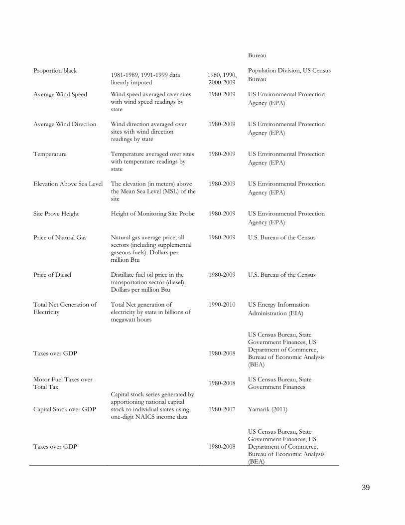
39

Bureau

Proportion black 1981-1989, 1991-1999 data linearly imputed

1980, 1990, 2000-2009

Population Division, US Census Bureau

Average Wind Speed Wind speed averaged over sites with wind speed readings by state


Average Wind Direction Wind direction averaged over sites with wind direction readings by state


Temperature Temperature averaged over sites with temperature readings by state


Elevation Above Sea Level The elevation (in meters) above the Mean Sea Level (MSL) of the site


Site Prove Height Height of Monitoring Site Probe 1980-2009 US Environmental Protection Agency (EPA)

Price of Natural Gas Natural gas average price, all sectors (including supplemental gaseous fuels). Dollars per million Btu

1980-2009

U.S. Bureau of the Census

Price of Diesel Distillate fuel oil price in the transportation sector (diesel). Dollars per million Btu

1980-2009 U.S. Bureau of the Census

Total Net Generation of Electricity

Total Net generation of electricity by state in billions of megawatt hours

1990-2010 US Energy Information Administration (EIA)

Taxes over GDP 1980-2008

US Census Bureau, State Government Finances, US Department of Commerce, Bureau of Economic Analysis (BEA)

Motor Fuel Taxes over Total Tax 1980-2008 US Census Bureau, State

Government Finances

Capital Stock over GDP

Capital stock series generated by apportioning national capital stock to individual states using one-digit NAICS income data

1980-2007 Yamarik (2011)

Taxes over GDP 1980-2008

US Census Bureau, State Government Finances, US Department of Commerce, Bureau of Economic Analysis (BEA)

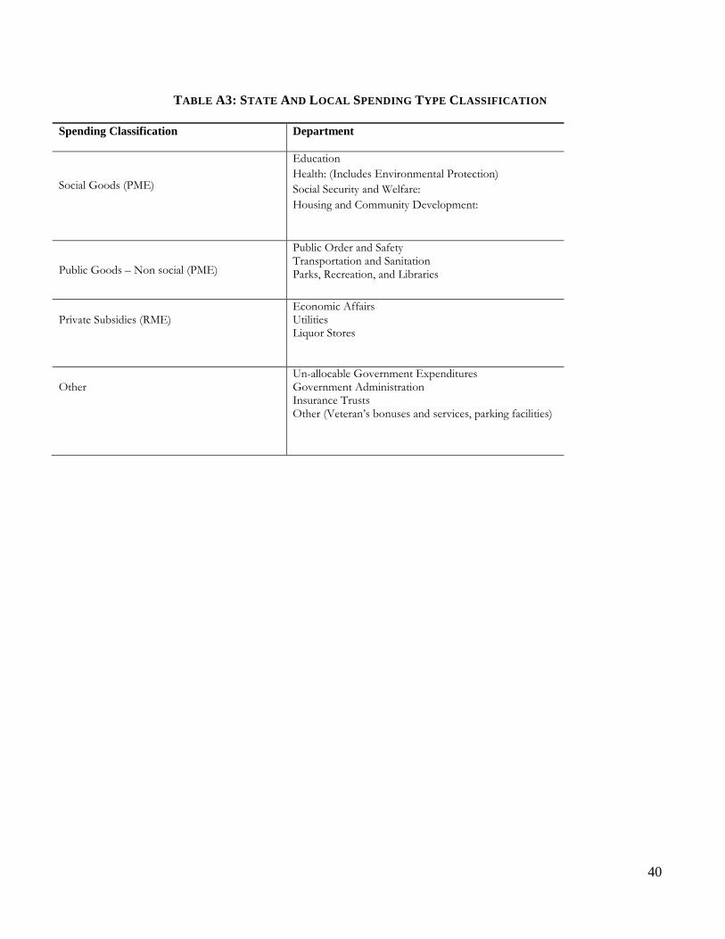
40

TABLE A3: STATE AND LOCAL SPENDING TYPE CLASSIFICATION

Spending Classification Department

Social Goods (PME)

Education Health: (Includes Environmental Protection) Social Security and Welfare: Housing and Community Development:

Public Goods – Non social (PME)

Public Order and Safety Transportation and Sanitation Parks, Recreation, and Libraries

Private Subsidies (RME)

Economic Affairs Utilities Liquor Stores

Other

Un-allocable Government Expenditures Government Administration Insurance Trusts Other (Veteran’s bonuses and services, parking facilities)

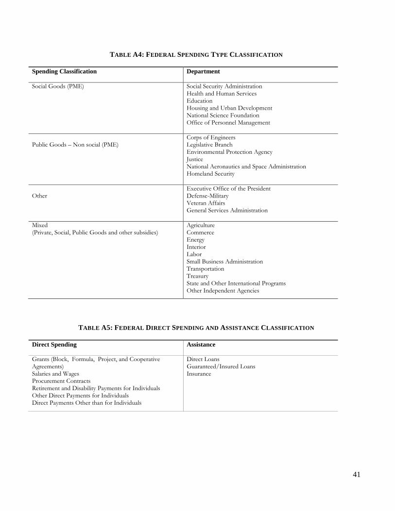
41

TABLE A4: FEDERAL SPENDING TYPE CLASSIFICATION

Spending Classification Department

Social Goods (PME) Social Security Administration Health and Human Services Education Housing and Urban Development National Science Foundation Office of Personnel Management

Public Goods – Non social (PME)

Corps of Engineers Legislative Branch Environmental Protection Agency Justice National Aeronautics and Space Administration Homeland Security

Other

Executive Office of the President Defense-Military Veteran Affairs General Services Administration

Mixed (Private, Social, Public Goods and other subsidies)

Agriculture Commerce Energy Interior Labor Small Business Administration Transportation Treasury State and Other International Programs Other Independent Agencies

TABLE A5: FEDERAL DIRECT SPENDING AND ASSISTANCE CLASSIFICATION

Direct Spending Assistance

Grants (Block, Formula, Project, and Cooperative Agreements) Salaries and Wages Procurement Contracts Retirement and Disability Payments for Individuals Other Direct Payments for Individuals Direct Payments Other than for Individuals

Direct Loans Guaranteed/Insured Loans Insurance

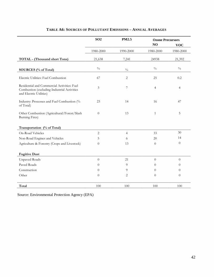
42

TABLE A6: SOURCES OF POLLUTANT EMISSIONS – ANNUAL AVERAGES

SO2 PM2.5 Ozone Precursors NO VOC

1980-2000 1990-2000 1980-2000 1980-2000 TOTAL - (Thousand short Tons) 21,638 7,241 24938 21,392

SOURCES (% of Total) % % % % Electric Utilities: Fuel Combustion

67

2

25

0.2

Residential and Commercial Activities: Fuel Combustion (excluding Industrial Activities and Electric Utilities)

3 7 4 4

Industry: Processes and Fuel Combustion (% of Total)

23 14 16 47

Other Combustion (Agricultural/Forest/Slash Burning Fires)

0 13 1 5

Transportation (% of Total) On-Road Vehicles 2 4 33 30

Non-Road Engines and Vehicles 5 6 20 14

Agriculture & Forestry (Crops and Livestock) 0 13 0 0

Fugitive Dust Unpaved Roads 0 21 0 0 Paved Roads 0 9 0 0 Construction 0 9 0 0 Other 0 2 0 0 Total 100 100 100 100

Source: Environmental Protection Agency (EPA)

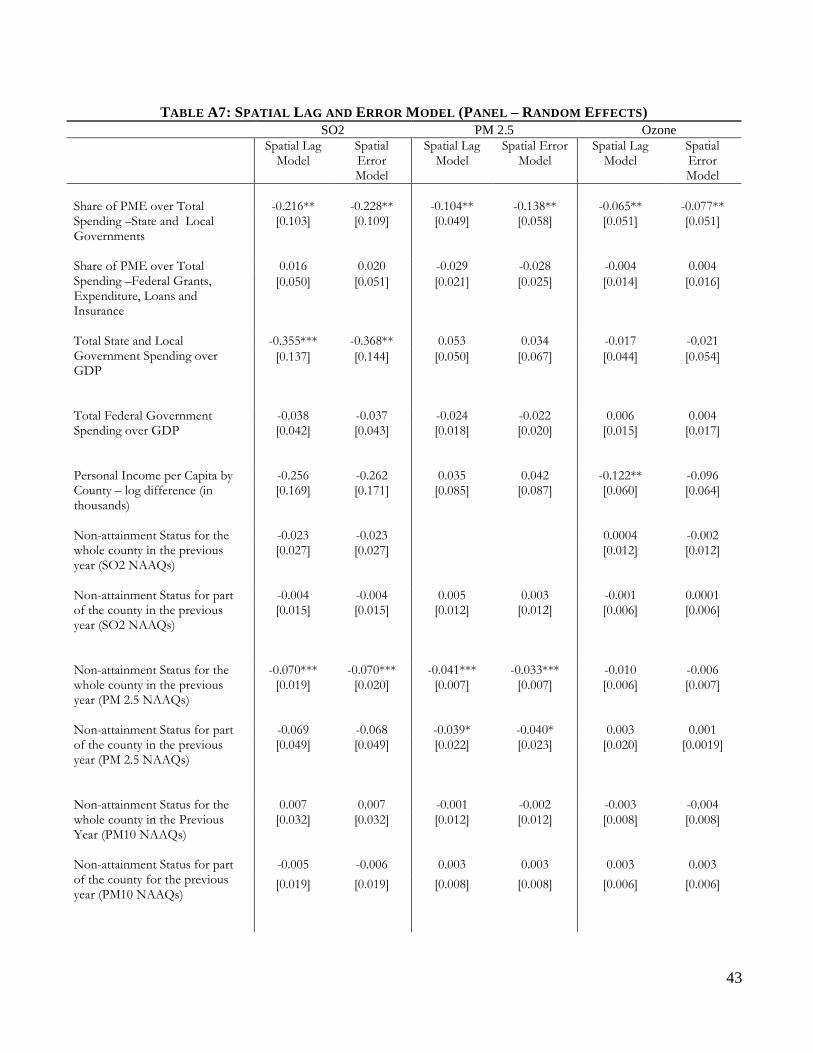
43

TABLE A7: SPATIAL LAG AND ERROR MODEL (PANEL – RANDOM EFFECTS) SO2 PM 2.5 Ozone Spatial Lag

Model Spatial Error Model

Spatial Lag Model

Spatial Error Model

Spatial Lag Model

Spatial Error Model


-0.216**

-0.228**

-0.104**

-0.138**

-0.065**

-0.077**

[0.103] [0.109] [0.049] [0.058] [0.051] [0.051]


0.016 0.020 -0.029 -0.028 -0.004 0.004 [0.050] [0.051] [0.021] [0.025] [0.014] [0.016]


-0.355*** -0.368** 0.053 0.034 -0.017 -0.021 [0.137] [0.144] [0.050] [0.067] [0.044] [0.054]


-0.038 -0.037 -0.024 -0.022 0.006 0.004 [0.042] [0.043] [0.018] [0.020] [0.015] [0.017]


-0.256 -0.262 0.035 0.042 -0.122** -0.096 [0.169] [0.171] [0.085] [0.087] [0.060] [0.064]


-0.023 -0.023 0.0004 -0.002 [0.027] [0.027] [0.012] [0.012]


-0.004 -0.004 0.005 0.003 -0.001 0.0001 [0.015] [0.015] [0.012] [0.012] [0.006] [0.006]


-0.070*** -0.070*** -0.041*** -0.033*** -0.010 -0.006 [0.019] [0.020] [0.007] [0.007] [0.006] [0.007]


-0.069 -0.068 -0.039* -0.040* 0.003 0.001 [0.049] [0.049] [0.022] [0.023] [0.020] [0.0019]


0.007 0.007 -0.001 -0.002 -0.003 -0.004 [0.032] [0.032] [0.012] [0.012] [0.008] [0.008]


-0.005 -0.006 0.003 0.003 0.003 0.003 [0.019] [0.019] [0.008] [0.008] [0.006] [0.006]

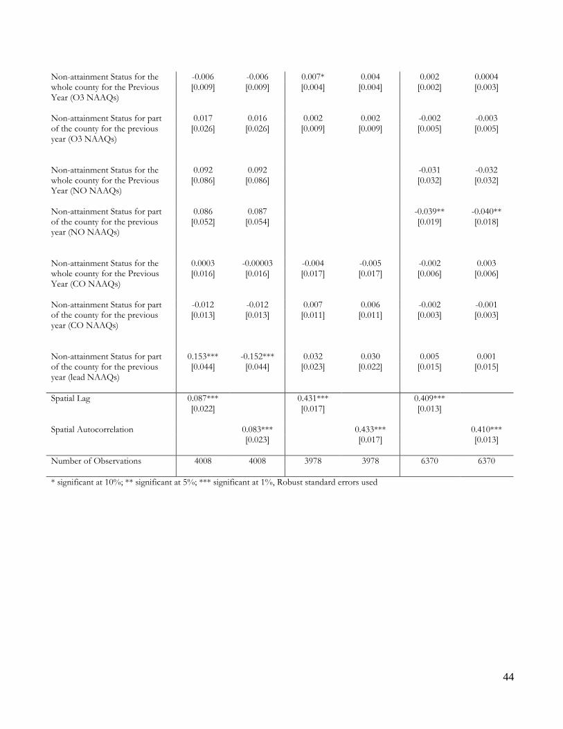
44

Non-attainment Status for the whole county for the Previous Year (O3 NAAQs)

-0.006 -0.006 0.007* 0.004 0.002 0.0004 [0.009] [0.009] [0.004] [0.004] [0.002] [0.003]


0.017 0.016 0.002 0.002 -0.002 -0.003 [0.026] [0.026] [0.009] [0.009] [0.005] [0.005]


0.092 0.092 -0.031 -0.032 [0.086] [0.086] [0.032] [0.032]


0.086 0.087 -0.039** -0.040** [0.052] [0.054] [0.019] [0.018]


0.0003 -0.00003 -0.004 -0.005 -0.002 0.003 [0.016] [0.016] [0.017] [0.017] [0.006] [0.006]


-0.012 -0.012 0.007 0.006 -0.002 -0.001 [0.013] [0.013] [0.011] [0.011] [0.003] [0.003]


0.153*** -0.152*** 0.032 0.030 0.005 0.001 [0.044] [0.044] [0.023] [0.022] [0.015] [0.015]

Spatial Lag

0.087*** 0.431*** 0.409*** [0.022] [0.017] [0.013]

Spatial Autocorrelation 0.083*** 0.433*** 0.410*** [0.023] [0.017] [0.013]

Number of Observations 4008 4008 3978 3978 6370 6370 * significant at 10%; ** significant at 5%; *** significant at 1%, Robust standard errors used