0263–8762/03/$23.50+0.00# Institution of Chemical Engineers

www.ingentaselect.com=titles=02638762.htm Trans IChemE, Vol 81, Part A, January 2003

MODELLING SIEVE TRAY HYDRAULICS USINGCOMPUTATIONAL FLUID DYNAMICS

R. KRISHNA and J. M. VAN BATENDepartment of Chemical Engineering, University of Amsterdam, Amsterdam, The Netherlands

T he ability of computational � uid dynamics (CFD) to model the complex two-phasehydrodynamics of sieve trays is examined. The key to a proper description of the � owis the estimation of the momentum exchange, or drag, coef� cient between the gas and

liquid phases. In the absence of sound theoretical models, empirical correlations for the averagegas fraction on the tray, such as those of Bennet, Agrawal and Cook [AIChE J, 29 (1983): 434],can be used to estimate the drag coef� cient. Transient simulations of sieve trays of 0.3 and0.9 m in diameter, operating in the bubbly � ow regime, reveal the chaotic, three-dimensionalcharacter of the � ow and the existence of circulation patterns in all three dimensions. The CFDsimulations underline the limitations of simpler approaches wherein the � ow is assumed to betwo-dimensional or where the interaction of the liquid phase with the gas phase is eitherignored completely or simpli� ed greatly. The major advantage of the CFD approach is thatgeometry and scale effects are properly encapsulated and do not require further inputs. It isconcluded that CFD can be a powerful investigative and design tool for sieve tray columns.

Keywords: computational � uid dynamics; sieve trays; clear liquid height; froth height; frothdensity; scale effects; liquid circulations.

INTRODUCTION

Distillation is the most widely used separation technique andis usually the � rst choice for separating mixtures. Only whendistillation fails does one look for other separation alterna-tives. One of the major factors that favours distillation is thefact that large-diameter columns can be designed and builtwith con� dence. Sieve tray distillation columns are widelyused in industrial practice and the description of the hydro-dynamics of sieve trays is of great importance. A properprediction of the sieve tray hydraulics is necessary for theprediction of separation ef� ciency and overall tray perfor-mance. For a given set of operating conditions (gas and liquidloads), tray geometry (column diameter, weir height, weirlength, diameter of holes, fractional hole area, active bub-bling area, downcomer area) and system properties, it isnecessary to predict the � ow regime prevailing on the tray,liquid hold-up, clear liquid height, froth density, interfacialarea, pressure drop, liquid entrainment, gas and liquid phaseresidence time distributionsand the mass transfer coef� cientsin either � uid phase. A lack of in-depth understanding of theprocesses occurring within a distillation column is a signi� -cant barrier to the further improvement of equipment perfor-mance. In 1986, in the preface to his in� uential book, Lockett(1986) wrote ‘Sieve tray decks are, after all, hardly more thansheets of metal with a few holes punched in them. This ofcourse is part of the fascination—that the behaviour of some-thing so simple can be so dif� cult to predict with regards to itshydrodynamic and mass transfer performance.’ Design ofsieve tray distillation columns is essentially empirical in

nature (Kister, 1992; Lockett, 1986; Stichlmair and Fair,1998; Zuiderweg, 1982).

In recent years, there has been considerable academic andindustrial interest in the use of computational � uid dynamics(CFD) to model two-phase � ows in process equipment(Krishna and Van Baten, 2001a). CFD techniques havebeen used to model bubble formation and rise in liquidsand powders (Krishna and Van Baten, 1999; Krishna et al.,2000a) and to describe the hydrodynamics of bubblecolumns (Borchersger et al., 1999; Krishna et al., 2000b)and � uidised beds (Krishna and Van Baten, 2001b; VanWachem et al., 2001). An important advantage of CFDtechniques is that geometry and scale effects are ‘automa-tically’ accounted for (Krishna et al., 2000b; Krishna andVan Baten, 2001a).

There have been some recent attempts to model sieve trayhydrodynamics using CFD (Liu et al., 2000; Krishna et al.,1999; Mehta et al., 1998; Van Baten and Krishna, 2000; VanBaten et al., 2001a,b). Mehta et al. (1998) analysed theliquid phase � ow patterns on a sieve tray by solving thetime-averaged equations of continuity of mass and momen-tum only for the liquid phase. Interactions with the vapourphase are taken account of by use of interphase momentumtransfer coef� cients determined from empirical correlations.Liu et al. (2000) attempt to model the two-phase � owbehaviour using a two-dimensional model, focussing onthe description of the hydrodynamics along the liquid � owpath, ignoring the variations in the direction of gas � owalong the height of the dispersion. Van Baten et al. (VanBaten and Krishna, 2000; Van Baten et al., 2001a,b) use

27

fully three-dimensional transient simulations to describe thehydrodynamics of sieve trays.

The objective of the present communication is to examinethe power, and limitations of CFD techniques in describingsieve tray hydraulics.We reviewand extendour previousCFDapproach (Krishna et al., 1999;Van Baten and Krishna, 2000;Van Baten et al., 2001a,b) to the description of liquid phaseresidence time distribution (RTD) and the in� uence of scaleeffects. We begin with a two-dimensional analysis of liquidphase channelling and bypassing on a tray.

TWO-DIMENSIONAL CFD ANALYSIS OFLIQUID PHASE CHANNELLING

Before attempting to model the complex gas–liquid trayhydrodynamics, let us consider CFD simulation of a simplecase of � ow of liquid across a round tray with the dimen-sions speci� ed in Figure 1(a). A total of 48 £ 60 ˆ 2880 gridcells of warped con� guration are used to cover the traygeometry. The liquid load per unit weir length is taken to be8.25 £ 10¡4 m3s¡1 m¡1, corresponding to an inlet liquidvelocity of 0.055 m s¡1. The mass and momentum conser-vation equations are:

@rL

@t‡ H ¢ …rLuL† ˆ 0 …1†

@rLuL

@t‡ H ¢ rLuLuL ¡ mL‰HuL ‡ …HuL†T Š

© ª

ˆ ¡Hp ‡ rLg …2†

where rL, uL and mL represent, respectively, the macroscopicdensity, velocity and viscosity of the liquid phase, p is thepressure, and g is the gravitational acceleration. The turbu-lent contribution to the stress tensor is evaluated by meansof low Reynolds number variant of the k–e model (Launderand Sharma, 1974), using standard single-phase parametersCm ˆ 0.09, C1e ˆ 1.44, C2e ˆ 1.92, skˆ 1 and se ˆ 1.3.

A commercial CFD package CFX 4.2 of AEATechnology,Harwell, UK, was used to solve equations (1) and (2) ofcontinuity and momentum. This package is a � nite volumesolver, using body-� tted grids. Discretization of theequations at the grid is performed using a � nitedifferencing (� nite volume) method. Physical space ismapped to a rectangular computational space. Velocityvector equations are treated as scalar equations, one scalarequation for each velocity component. All scalar variablesare discretised and evaluated at the cell centres. Velocitiesrequired at the cell faces are evaluated by applying animproved Rhie and Chow (1983) interpolation algorithm.Transport variables such as diffusion coef� cients and effec-tive viscosities are evaluated and stored at the cell faces. Thepressure–velocity coupling is obtained using the SIMPLECalgorithm (Van Doormal and Raithby, 1984). For the convec-tive terms in equations (1) and (2), hybrid differencing wasused. The transient equations were solved with 0.01 s timesteps until steady state was reached. A fully implicit back-ward differencing scheme was used for the time integration.

The steady-statevelocity pro� les are shown in Figure 1(b).The recirculation patterns in the rounded segments of thetray are evident. Such recirculation patterns were � rsthighlighted in the classic paper of Porter et al. (1972). Wenote from Figure 1(b) that the liquid velocity in the central� ow path is about 0.06 m s¡1, whereas the liquid is practi-

cally at a standstill in a major portion of rounded segments.CFD simulations can also be used to determine the residencetime distribution by injecting a pulse tracer and monitoringits progression as it moves through the tray. Snapshots of thetracer movement are shown in Figure 2. It is clearly seenthat, while the tracer concentration has reduced to practicallyzero in the central rectangular region within 8 s of tracerinjection, it is swished to the rounded segmental regions andlingers there for a very long time. The normalized RTD isshown in Figure 3. The tracer response cannot be describedby an axial dispersion model; on the other hand a model withN stirred tanks in series, exchanging tracer with a deadspace, is able to match the tracer response very well; see thecontinuous lines in Figure 3. The best � t with the CFDsimulations is obtained taking the number of stirred tanksN ˆ 40 and the dead space volume to be 28% of the totaltray volume. The exchange between the active and the deadzone amounts to only 0.004 of the inlet � ow. From geometryconsiderations, the rounded segmental portions are 32% ofthe total tray volume; this is in close agreement with thedead zone determined from CFD simulations.

There are clear limitations of the above analysis, assum-ing two-dimensional � ow of only liquid across the tray. Thisis because the introduction of the gas phase will have asigni� cant in� uence on the recirculation patterns. Further-more, the gas–liquid hydrodynamics assumes a truly chaoticnature, as we shall see below.

THREE-DIMENSIONAL SIMULATION STRATEGYFOR GAS±LIQUID HYDRODYNAMICS

There are many � ow regimes on sieve trays (Lockett,1986), ranging from gas-dispersed bubbly � ow regime toliquid-dispersed spray � ow regime; see Figure 4. From aCFD point of view, the bubbly � ow regime is mucheasier to describe and model than the spray � ow regimebecause it is easier to model the gas–liquid drag whichis much more uniform along the dispersion height. Onthe other hand, in the spray � ow regime, the gas–liquiddrag can be expected to vary signi� cantly up thedispersion, making the modelling much more dif� cult.We therefore restrict ourselves to the description of thebubbly � ow regime. The derivation of the basic equa-tions for dispersed two-phase � ows is discussed byJakobsen et al. (1997) and here we present a summary.For either gas (subscript G) or liquid (subscript L)phases in the two-phase dispersion on the tray thevolume-averaged mass and momentum conservationequations are given by:

@…eGrG†@t

‡ H ¢ …rGeGuG† ˆ 0 …3†

@…eLrL†@t

‡ H ¢ …rLeLuL† ˆ 0 …4†

@…rGeGuG†@t

‡ H ¢ rGeGuGuG ¡ mGeG‰HuG ‡ …HuG†TŠ© ª

ˆ ¡eGHp ‡ MG;L ‡ rGeGg …5†@…rLeLuL†

@t‡ H ¢ rLeLuLuL ¡ mLeL‰HuL ‡ …HuL†TŠ

© ª

ˆ ¡eLHp ¡ MG;L ‡ rLeLg …6†

Trans IChemE, Vol 81, Part A, January 2003

28 KRISHNA and VAN BATEN

where rk, uk, ek and mk represent, respectively, the macro-scopic density, velocity, volume fraction and viscosity of thephase k, p is the pressure, MG,L, the interphase momentumexchange between gas and liquid phases and g is the gravita-tional acceleration. The gas and liquid phases share the samepressure � eld, pGˆ pLˆ p. The added mass force has beenignored in the present analysis. Lift forces are also ignored inthe present analysis because of the uncertainty in assigningvalues of the lift coef� cients. For the continuous, liquid,phase, the turbulent contribution to the stress tensor isevaluated by means of k–e model, using standard single-phaseparameters. No turbulencemodel is used for calculatingthe velocity � elds of the dispersed gas bubbles in the bubbly� ow regime.

The interphase momentum exchange term is:

ML;G ˆ 34

rLeG

dGCD…uG ¡ uL†juG ¡ uLj …7†

where CD is the interphase momentum exchange coef� cientor drag coef� cient. The proper estimation of the dragcoef� cient is the key to the successful modelling of thetray hydraulics. For the Stokes regime:

CD ˆ 24=ReG; ReG ˆ rLUGdG=mL …8†

and for the inertial regime, also known as the turbulentregime:

CD ˆ 0:44 …9†

For the churn-turbulent regime of bubble column operation(Krishna et al., 2000b; Krishna and Van Baten, 2001a) thedrag coef� cient for a swarm of large bubbles is estimatedusing:

CD ˆ 43

rL ¡ rG

rLgdG

1V 2

slip…10†

where Vslip is the slip velocity of the bubble swarm withrespect to the liquid:

Vslip ˆ juG ¡ uLj …11†

Substituting equation (10) into equation (7) we � nd:

ML;G ˆ eG…rL ¡ rG†g 1V 2

slip

…uG ¡ uL†juG ¡ uLj …12†

The slip between gas and liquid can be estimated fromsuper� cial gas velocity UG and the gas hold-up eG:

Vslip ˆ UG=eG …13†

An empirical correlation for the gas fraction on the tray as afunction of the super� cial gas velocity can be used to theestimate the slip velocity. In this work, we use the Bennettet al. (1983) correlation to estimate the gas hold-up:

eBL ˆ exp ¡12:55 UG

�����������������rG

rL ¡ rG

r³ ´0:91" #

; eBG ˆ 1 ¡ eB

L

…14†

It is important to note that the Bennett correlation does notinclude tray geometry or scale parameters. The interphasemomentum exchange term is therefore:

ML;G ˆ eG…rL ¡ rG†g 1

…UG=eBG†2 …uG ¡ uL†juG ¡ uLj

…15†

This formulation, however, gives numerical dif� cultiesbecause in the freeboard the liquid hold-up is zero. In orderto overcome this problemwe modify equation(15) as follows:

ML;G ˆeGeL…rL¡rG†g 1

…UG=eBG†2

1eBL

" #…uG ¡uL†juG¡uLj

…16†

where the term

1

…UG=eBG†2

1eBL

" #

is estimated a priori from the Bennett relation, equation(14), and the desired gas velocity. This approach ensuresthat the average gas hold-up in the gas–liquid dispersion onthe froth conforms to experimental data over a wide range ofconditions (as measured by Bennett et al., 1983). Whenincorporating equation (16) for the gas–liquid momentumexchange within the momentum balance relations (5) and(6), the local transient, values of uG, uL, eG and eL are used.A further point to note is that use of equation (16) for themomentum exchange obviates the need for specifying thebubble size. Indeed, for the range of super� cial gasvelocities used in our simulations to be reported below,0.5–0.9 m s¡1, we do not expect well-de� ned bubbles. Thetwo-phase Eulerian simulation approach used here onlyrequires that the gas phase is the dispersed phase; thisdispersion could consist of either gas bubbles or gas jets,or a combination thereof.

Figure 5 shows the con� guration of the system that hasbeen simulated. The diameter of the tray is 0.3 m with aheight of 0.12 m. The length of the weir is 0.18 m, giving a� ow path length of 0.24 m. The chosen height of 0.12m issuf� cient to prevent liquid carryover out of the computa-tional space. The liquid enters the tray through a rectangularopening that is 0.015 m high. The height of the weir isvaried in the simulations and has the values of 60, 80 and100 mm. The total number of grid cells used in the simula-tions is 48 £ 60 £ 24 ˆ 69,120; 48 cells in liquid � owdirection, 60 cells in direction perpendicular to the liquid� ow and 24 cells in the vertical direction. Figure 6 shows thelayout of the distributor grid, which consists of 180 holes.The choice of the grid size is based on our experiencegained in the modelling of � uidized beds and gas–liquidbubble columns operating in the churn-turbulent regime(Krishna et al., 2000b; Krishna and Van Baten, 2001a,b).The use of warped square holes does not impact on thesimulation results, because we use the Eulerian frameworkfor describing either � uid phase.

Trans IChemE, Vol 81, Part A, January 2003

MODELLING SIEVE TRAY HYDRAULICS 29

Air, at ambient pressure conditions, and water were usedas the gas and liquid phases respectively. At the start of asimulation, the tray con� guration shown in Figure 5 is � lledwith a uniform gas–liquid dispersion, with 10% gas holdup,up to the height of the weir and gas is injected throughthe holes at the distributor. The time increment used in thesimulations is 0.002 s. During the simulation, the volumefraction of the liquid phase in the gas–liquid dispersion inthe system is monitored and quasi-steady state is assumed toprevail if the value of the hold-up remains constant for aperiod long enough to determine the time-averaged valuesof the various parameters. For obtaining the values of theclear liquid height, gas holdup of dispersion, etc., theparameter values are averaged over a suf� ciently longperiod over which the holdup remains steady.

Simulations have been performed on a Silicon GraphicsPower Challenge with six R10000 processors running at200 MHz. A typical simulation took about 4 days tosimulate 20 s of tray hydrodynamics. From the simulationresults, average liquid hold-up as a function of height hasbeen determined. Clear liquid height has been determinedby multiplying the average liquid hold-up with the height ofthe computational space (0.12m). Further computationaldetails of the algorithms used, boundary conditions, includinganimations are available on our web site (http://ct-cr4.chem.uva.nl/sievetrayCFD/).

Let us � rst consider snapshots, at 5 s intervals, of themovement of liquid along the � ow path and over the weir;see Figures 7 and 8. Near the bottom of the tray, the liquid isdrawn toward the centre and is dragged up vertically by thegas phase. The liquid disengages itself from the dispersedgas phase and travels down the sides, resulting in circulationcells that are evident in both the front (Figure 7) and weir(Figure 8) views. The snapshots also re� ect the chaoticnature of the � ow. There are two circulation cells whenviewed from the front and from the weir.

Snapshots of the liquid � ow patterns viewed 10 and40 mm above the tray � oor are shown in Figure 9. Near thebottom of the tray the liquid is drawn inward and carriedupwards; this is evidenced by the fact that all the liquidvelocity vectors are pointing inwards; see 10 mm view atthe top of the Figure 9. Liquid recirculations are clearlyvisible in the 40 mm view at the bottom of Figure 9. Thecirculation patterns clearly have a chaotic character. Whenthe transient simulations are time-averaged, the liquidphase velocity vectors at 40 mm above the tray areobtained as shown in Figure 10. The recirculation cellsat the rounded segments are clearly seen. However, it isinteresting to note that the liquid velocity is directedtowards the centre; this is because of the circulation cellsseen in the front and weir views in Figures 7 and 8respectively. The liquid phase circulations with gas � owhave therefore a totally different character than without gas� ow (Figure 2).

Figure 11 presents typical simulation results for thevariation of the liquid hold-up along the height of thedispersion. The values of the hold-up are obtainedafter averaging along the x- and y-directions and over asuf� ciently long time interval once quasi-steady-stateconditions are established. The simulated trends in theliquid hold-up as a function of the gas velocity UG are inline with literature information (Hofhuis and Zuiderweg,1979).

Figure 12 (a)–(c) compares the calculations of the clearliquid height from CFD simulations with the Bennett et al.(1983) correlation:

hcl ˆ eBL hw ‡ C

QL

W eBL

³ ´0:67" #

;

C ˆ 0:50 ‡ 0:438 exp…¡137:8hw† …17†

where eLB is determined from equation (14). It must be

emphasized that equation (17) is entirely independent ofthe holdup correlation presented in equation (14). Putanother way, the incoporation of the holdup correlationinto our CFD inputs does not imply anything by way ofinformation on the clear liquid height. The values of theclear liquid height from the simulations are obtained afteraveraging over a suf� ciently long time interval once quasi-steady-state conditions are established and determining thecumulative liquid hold-up within the computational space. Itis remarkable to note that the clear liquid height determinedfrom the CFD simulations matches the Bennett correlationquite closely, even though no in� uence of the weir height orliquid weir load on the interface gas–liquid momentumexchange coef� cient has been used in the model. Geometryeffects are properly taken account of in the CFD approach.

We have also studied the residence time distribution(RTD) of liquid phase by following the course of a tracer(red colour) in the liquid entering at the inlet to the tray. Inorder to gain insight into the tracer movement in the liquidphase, let us consider a speci� c tray operation at UGˆ0.7 m s¡1, weir height hwˆ 80 mm; liquid load QL=W ˆ8.25 £ 10¡4 m3 s¡1 m¡1. Snapshots of the tracer concentra-tions at various time steps from start of the pulse tracer areshown in Figure 13. In sharp contrast to the correspondingtwo-dimensional liquid simulations shown in Figure 3, wenote that there is no starvation of tracer at the segmentalregions; the tracer appears to be dispersed over the wholetray cross section. Put another way, the chaotic gas–liquidhydrodynamics leads to good tracer dispersion.

The major advantage of CFD simulations is that scaleeffects are captured. In order to illustrate this, let us considersimulations of at 0.9 m diameter tray operating at UGˆ0.7 m s¡1, weir height hwˆ 80 mm; liquid load QL=W ˆ8.25 £ 10¡4 m3 s¡1 m¡1. A total of 622,080 cells arerequired to capture the hydrodynamics. A snapshot of thefront view of the tray shows the existence of multiple cells,four in number, in the � ow direction; see Figure 14(a). Thisis in sharp contrast to the 0.3 m diameter tray, whichdisplayed only two circulation cells in the � ow direction.The weir view of the tray also shows the existence of fourcirculation cells; see Figure 14(b).

When the 0.9 m tray is viewed from the top at a position40 mm above the tray � oor, we again note a multiplicity ofcirculation patterns; see Figure 15. It is clear that, asthe column diameter increases, so do the number of circula-tion cells. This implies that the liquid phase will be morebackmixed in columns of smaller diameter. The liquid phasein large diameter columns will approach plug � ow character.

The time averaged clear liquid height, hcl, for the 0.9 mtray after quasi-steady state has been achieved is almostidentical to that of the 0.3 m diameter tray; the simulationresults are compared in Figure 12. There is a small scaleeffect with regard to clear liquid height and gas holdup on

Trans IChemE, Vol 81, Part A, January 2003

30 KRISHNA and VAN BATEN

the tray. The mixing character of the liquid phase is,however, profoundly in� uenced by the scale, as has beenemphasized above.

HYDRODYNAMICS OF SIEVE TRAYS WITHCATALYST CONTAINERS

There is a great deal of industrial interest in reactivedistillation (Taylor and Krishna, 2000). For heterogeneously

catalysed liquid phase reactions, the liquid phase has to bebrought into intimate contact with catalyst particles. Bothpacked columns (random packed or structured) and traycolumns could be used. In order to avoid diffusional limita-tions, the catalyst particles have to be smaller than about3 mm in size. Such catalyst particles are usually encasedwithin wire-gauze envelopes as in the KATAPAK-S andKATAMAX constructions of Sulzer Chemtech and Koch-Glitsch. An alternative to the KATAPAK-S and KATAMAXconstruction is to dispose the wire gauze parcels containing

Figure 1. Two-dimensional simulation of liquid � ow across a tray of 0.3 m diameter. (a) Computational grid. (b) Steady-state velocity pro� les shown incolour scale.

Figure 2. Snapshots showing the movement of colour tracer across the tray. Highest tracer concentration is denoted by red. Blue areas do not contain tracer.The shades of colours in between blue (zero tracer concentration) and red (highest tracer concentration) denote the tracer concentrations.

Trans IChemE, Vol 81, Part A, January 2003

MODELLING SIEVE TRAY HYDRAULICS 31

catalyst along the liquid � ow direction of a sieve traydistillation column as shown in Figure 16. The liquidhold-up is usually much higher in sieve tray columns ascompared to packed columns and this is an advantage whencarrying out relatively slow, catalysed, liquid phase reac-tions. A further advantage of a catalytic sieve tray construc-tion is that the contacting on any tray is cross-current andfor large diameter columns there will be a high degree of

staging in the liquid phase; this is advantageous from thepoint of view of selectivity and conversion. There is verylittle published information on the hydrodynamics of suchcontacting devices. CFD simulations are particularly suitedto describe the hydrodynamics, because the preferred regimeof operation in reactive distillation tray columns is thebubbly � ow regime, which is well described in CFD, asseen in the foregoing.

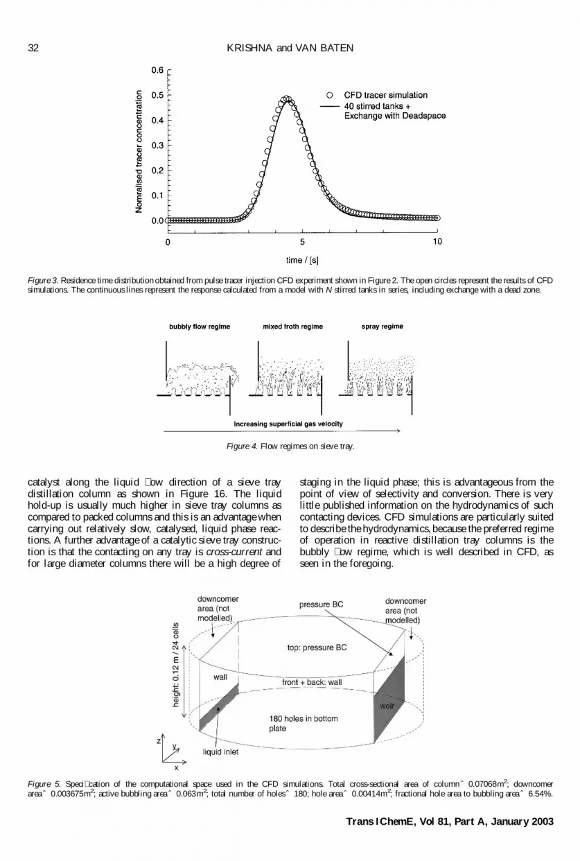
Figure 3. Residence time distribution obtained from pulse tracer injection CFD experiment shown in Figure 2. The open circles represent the results of CFDsimulations. The continuous lines represent the response calculated from a model with N stirred tanks in series, including exchange with a dead zone.

Figure 4. Flow regimes on sieve tray.

Figure 5. Speci� cation of the computational space used in the CFD simulations. Total cross-sectional area of column ˆ 0.07068m2; downcomerarea ˆ 0.003675m2; active bubbling area ˆ 0.063m2; total number of holesˆ 180; hole area ˆ 0.00414m2; fractional hole area to bubbling area ˆ 6.54%.

Trans IChemE, Vol 81, Part A, January 2003

32 KRISHNA and VAN BATEN

The gas–liquid � ow in the open spaces between thecatalyst containers can be modelled in exactly the samemanner as before (van Baten et al., 2001a,b). When viewedfrom the front, the hydrodynamics has the same chaoticcharacter as before (see Figure 7), as is evidenced in thesnapshot shown in Figure 17(a). There tends to be accumu-lation of liquid on top of the catalyst containers; this isevidenced by the snapshot taken from the front, at a position25 mm off-centre; see Figure 17(b).

The liquid accumulation is clearly evident in the snapshottaken from the weir view; see Figure 17(c). The pro� les ofliquid holdup along the tray dispersion height shown inFigure 18, show clear differences with the correspondingsimulations without containers shown in Figure 11. Inpractice, this liquid accumulation can be prevented bytapering the top of the containers.

The presence of the liquid containers tends to dampen outthe circulation cells and the � ow along from the inlet to theweir has a more plug � ow character; this is evidenced by thetop view snapshot shown in Figure 19.

Good quantitative agreement between the CFD simula-tion results with catalyst containers and experimental resultsof Van Baten et al. (2001a,b) as is evidenced in thecomparison presented in Figure 20. The experiments havebeen performed in a rectangular tray rather than in a roundtray (see http://ct-cr4.chem.uva.nl/kattray/).

Figure 6. Layout of the distributor plate used in the CFD simulations: totalnumber of holes ˆ 180; hole area ˆ 0.00414m2; fractional hole area tobubbling area ˆ 6.54%. The average area of one hole is 23 mm2.

Figure 7. Snapshots of the front view of 0.3 m sieve tray simulations at a super� cial gas velocity, UGˆ 0.7m s¡1; weir height hwˆ 80 mm; liquid weir loadQL=W ˆ 8.25£ 10¡4m3s¡1m¡1. The colours indicate the liquid holdup (scale on the left).

Figure 8. Snapshots of the weir view of 0.3 m sieve tray simulations at a super� cial gas velocity, UGˆ 0.7 m s¡1; weir height hwˆ 80 mm; liquid weir loadQL=W ˆ 8.25£ 10¡4m3s¡1m¡1. The colours indicate the liquid holdup (scale on the left).

Trans IChemE, Vol 81, Part A, January 2003

MODELLING SIEVE TRAY HYDRAULICS 33

Figure 9. Snapshots of the top views, 10 and 40 mm above the � oor of the 0.3 m tray. Super� cial gas velocity, UGˆ 0.7 m s¡1; weir height hwˆ 80 mm; liquidweir load QL=Wˆ 8.25£ 10¡4m3s¡1m¡1. The colours indicate the liquid holdup (scale on the left).

Figure 10. Time-averaged liquid phase velocity vectors, 40 mm above the� oor of the 0.3 m tray. Super� cial gas velocity, UGˆ 0.7 m s¡1; weir heighthwˆ 80 mm; liquid weir load QL=W ˆ 8.25£ 10¡4m3s¡1m¡1.

Figure 11. Distribution of liquid holdup along the height of the dispersionfor super� cial gas velocities, UGˆ 0.5, 0.7 and 0.9 m s¡1. Weir heighthwˆ 80 mm; liquid weir load QL=W ˆ 8.25£ 10¡4m3s¡1m¡1. The valuesof the holdup are obtained after averaging along the x- and y-directions andover a suf� ciently long time interval once quasi-steady-state-conditions areestablished.

Trans IChemE, Vol 81, Part A, January 2003

34 KRISHNA and VAN BATEN

Figure 12. Clear liquid height as a function of the (a) super� cial gas velocity, (b) liquid load, and (c) weir height. Comparison of Bennett correlation with CFDsimulations for 0.3 m diameter tray. Also shown are CFD simulation results for 0.9 m tray (see below).

Figure 13. Snapshots of tracer concentration at various times after tracer injection, viewed from the top at 40 mm above the � oor of the 0.3 m tray. Super� cialgas velocity, UGˆ 0.7 m s¡1; weir height hwˆ 80 mm; liquid weir load QL=W ˆ 8.25£ 10¡4m3s¡1m¡1. The colours indicate the liquid tracer concentration(see scale). Further computational details of the algorithms used, boundary conditions, including animations, are available on our web site (http://ct-cr4.chem.uva.nl/sievetrayCFD/tracer/).

Figure 14. Snapshots of the (a) front view and (b) weir view of 0.9m sieve tray simulation at a super� cial gas velocity. UGˆ 0.7 m s¡1; weir heighthwˆ 80 mm; liquid weir load QL=Wˆ 8.25£ 10¡4m3s¡1m¡1. The colours indicate the liquid holdup (scale as in Figure 7). Further computational details ofthe algorithms used, boundary conditions, including animations are available on our web site (http://ct-cr4.chem.uva.nl/sievetrayCFD/big/).

Trans IChemE, Vol 81, Part A, January 2003

MODELLING SIEVE TRAY HYDRAULICS 35

Figure 15. Snapshots of the top view, 40 mm above the tray � oor, of 0.9 msieve tray simulation at a super� cial gas velocity. UGˆ 0.7 m s¡1; weirheight hwˆ 80 mm; liquid weir load QL=W ˆ8.25£ 10¡4m3s¡1m¡1. Thecolours indicate the liquid holdup (scale as in Figure 7). See also our website (http://ct-cr4.chem.uva.nl/sievetrayCFD/big/).

Figure 16. Computational space for CFD simulations 0.3 m diameter sievetray containing catalyst-� lled containers.

Figure 17. (a) Snapshots of the front view, (b) off-centre front view and (c)weir view of 0.3 m catalyst containing sieve tray simulations at a super� cialgas velocity. UGˆ 0.7 m s¡1; weir height hwˆ 80 mm; liquid weir loadQL=W ˆ 8.25£ 10¡4m3s¡1m¡1. The colours indicate the liquid holdup(scale as in Figure 7). Animations can be viewed on our web site (http://ct-cr4.chem.uva.nl/katsievetrayCFD/).

Figure 18. Simulation results with catalyst containers. Distribution of liquidholdup along the height of the dispersion for super� cial gas velocities.UGˆ 0.5, 0.7 and 0.9 m s¡1, weir height hwˆ 80 mm; liquid weir loadQL=W ˆ 8.25£ 10¡4m3s¡1m¡1. The corresponding simulation resultswithout catalyst containers are shown in Figure 11.

Figure 19. Snapshots of the top view of 0.3 m catalyst containing sieve traysimulations. Operating conditions as in legend to Figure 17.

Trans IChemE, Vol 81, Part A, January 2003

36 KRISHNA and VAN BATEN

CONCLUSIONS

We have discussed the modelling of the sieve tray hydro-dynamics using CFD. Approaches, neglecting the gas phaseand assuming the � ow to be two-dimensional in characterexaggerate the importance of dead zones. A fully three-dimensional transient simulation reveals the true three-dimensional and chaotic character with liquid circulationcells in both vertical and horizontal directions. The predic-tions of the clear liquid height and liquid hold-up from theCFD simulations show the right trends with varying super-� cial gas velocity, liquid weir load and weir height, andmatch the values of the Bennett et al. (1983) correlationquite closely. The existence of dead zones is unlikely inactual practice. CFD simulations are able to describe thechanges in the hydrodynamics with increasing scale.Comparing of the simulations of the 0.3 and 0.9 m diametertrays shows that the number of circulating cells increaseswith column diameter. This means that the liquid phase willtend to have a plug � ow character in large diameter trays.The column diameter has, however, a small effect on theclear liquid height and gas holdup on the tray.

CFD simulations are particularly helpful in describing thehydrodynamics of sieve trays containing internals such ascatalyst containing envelopes.

Our studies show that CFD simulations can be a power-ful investigative, and design tool for distillation trays. Thesuccess of the CFD technique is so far restricted tothe bubbly � ow regime. To describe the spray regime,more reliable models to represent the interphase dragcoef� cient will be required. This area requires furtherattention.

NOMENCLATURE

dG diameter of gas bubble, mC parameter used in the Bennett correlation (17)CD drag coef� cient, dimensionlessg acceleration due to gravity, 9.81m s¡2

g acceleration vector due to gravityhcl clear liquid height, mhw weir height, mh position along height, mM interphase momentum exchange term, N m¡3

p pressure, N m¡2

QL liquid � ow rate across tray, m3s¡1

Re Reynolds number, dimensionlesst time, s

u velocity vector, m s¡1

UG super� cial gas velocity, m s¡1

Vslip slip velocity between gas and liquid, m s¡1

W weir length, mx coordinate, my coordinate, mz coordinate, m

Greek symbolse volume fraction of phase, dimensionlessm viscosity of phase, Pa sr density of phases, kg m¡3

Subscriptscl clear liquidG referring to gas phasek index referring to one of the phasesL referring to liquid phaseslip slipSuperscriptsB from Bennett correlation

REFERENCES

Bennett, D.L., Agrawal, R. and Cook, P.J., 1983, New pressure dropcorrelation for sieve tray distillation columns, AIChE J, 29: 434–442.

Borchersger, O., Busch, C., Sokolichin, A. and Eigenberger, G., 1999,Applicability of the standard k–e turbulence model to the dynamicsimulation of bubblecolumns: part II: comparison of detailed experimentsand � ow simulations, Chem Engng Sci, 54: 5927–5935.

Hofhuis, P.A.M. and Zuiderweg, F.J., 1979, Sieve plates: dispersion densityand � ow regimes, Inst Chem Engrs Symp Ser, 56: 2.2/1–2.2/26.

Jakobsen, H.A., Sannæs, B.H., Grevskott, S. and Svendsen, H.F., 1997,Modeling of bubble driven vertical � ows, Ind Engng Chem Res, 36:4052–4074.

Kister, H.Z., 1992, Distillation Design (McGraw-Hill, New York, USA).Krishna, R. and Van Baten, J.M., 1999, Simulating the motion of gas bubbles

in a liquid, Nature, 398: 208.Krishna, R. and Van Baten, J.M., 2001a, Scaling up bubble column reactors

with the aid of CFD, Trans IChemE Part A, Chem Eng Res Des, 79: 283–309.

Krishna, R. and Van Baten, J.M., 2001b,Using CFD for scaling up gas–solidbubbling � uidised bed reactors with Geldart A powders, Chem Engng J,82: 247–257.

Krishna, R., Van Baten, J.M., Ellenberger, J., Higler, A.P. and Taylor, R.,1999, CFD simulations of sieve tray hydrodynamics, Trans IChemE PartA, Chem Eng Res Des, 77: 639–646.

Krishna, R., Van Baten, J.M., Urseanu, M.I. and Ellenberger, J., 2000a, Risevelocity of single circular-cap bubbles in two-dimensional beds ofpowders and liquids, Chem Engng Process, 39: 433–440.

Krishna, R., Van Baten, J.M. and Urseanu, M.I., 2000b, Three-phaseEulerian simulations of bubble column reactors operating in the churn-turbulent � ow regime: a scale up strategy, Chem Engng Sci, 55:3275–3286.

Figure 20. Experiments vs CFD simulations for hydrodynamics of sieve trays with catalyst containers. Clear liquid height as a function of the (a) super� cialgas velocity, (b) liquid load, and (c) weir height. The experiments have been performed in a rectangular tray rather than in a round tray (see http://ct-cr4.chem.uva.nl/kattray/).

Trans IChemE, Vol 81, Part A, January 2003

MODELLING SIEVE TRAY HYDRAULICS 37

Launder, B.E. and Sharma, B.T., 1974, Application of the energy dissipationmodel of turbulence to the calculation of � ow near a spinning disc, LettHeat Mass Transfer, 1: 131–138.

Liu, C.J., Yuan, X.G., Yu, K.T. and Zhu, X.J., 2000, A � uid dynamic modelfor � ow-pattern on distillation tray, Chem Engng Sci, 55: 2287–2294.

Lockett, M.J., 1986, Distillation Tray Fundamentals (Cambridge UniversityPress, Cambridge, UK).

Mehta, B., Chuang, K.T. and Nandakumar, K., 1998, Model for liquid phase� ow on sieve trays, Trans IChemE Part A, Chem Eng Res Des, 76: 843–848.

Porter, K.E., Lockett, M.J. and Lim, C.T., 1972, The effect of liquidchannelling on distillation plate ef� ciency, Trans IChemE, 45: 91–101.

Rhie, C.M. and Chow, W.L., 1983, Numerical study of the turbulent � owpast an airfoil with trailing edge separation, AIAA J, 21: 1525–1532.

Stichlmair, J.G. and Fair, J.R., 1998, Distillation Principles and Practice(Wiley-VCH, New York).

Taylor, R. and Krishna, R., 2000, Modelling reactive distillation, ChemEngng Sci, 55: 5183–5229.

Van Baten, J.M. and Krishna, R., 2000, Modelling of sieve tray hydraulicsusing computational � uid dynamics, Chem Engng J, 77: 143–152.

Van Baten, J.M., Ellenberger, J. and Krishna, R., 2001a, Hydrodynamics ofreactive distillation tray column with catalyst containing envelopes:experiments vs CFD simulations, Catal Today, 66: 233–240.

Van Baten, J.M., Ellenberger, J. and Krishna, R., 2001b, Hydrodynamics ofdistillation tray column with structured catalyst containing envelopes:experiments vs CFD simulations, Chem Engng Technol, 24:077–1081.

Van Doormal, J. and Raithby, G.D., 1984, Enhancement of the SIMPLEmethod for predicting incompressible � ows, Numer Heat Transfer, 7:147–163.

Van Wachem, B.G.M., Schouten, J.C., van den Bleek, C.M., Krishna, R. andSinclair, J.L., 2001, Comparative analysis of CFD models for dense gas–solid systems, AIChE J, 47: 1035–1051.

Zuiderweg, F.J., 1982, Sieve trays. A view on the state of the art, ChemEngng Sci, 37: 1441–1464.

ACKNOWLEDGEMENT

The Netherlands Foundation for Scienti� c Research (NWO) is gratefullyacknowledged for providing � nancial assistance in the form of a program-masubsidie for development of novel concepts in reactive separationstechnology.

ADDRESS

Correspondence concerning this paper should be addressed to ProfessorR. Krishna, Department of Chemical Engineering, University of Amster-dam, Nieuwe Achtergracht 166, 1018 WV Amsterdam, The Netherlands.E-mail: krishna@science.uva.nl

The paper was a plenary lecture at the International Conference onDistillation and Absorption held in Baden-Baden, Germany, 30 September–2 October 2002. The manuscript was received 8 July 2002 and accepted forpublication after revision 8 November 2002.

Trans IChemE, Vol 81, Part A, January 2003

38 KRISHNA and VAN BATEN