The effects of mean atmospheric forcings of the stable atmospheric boundary layer onwind turbine wakeKiran Bhaganagar and Mithu Debnath Citation: Journal of Renewable and Sustainable Energy 7, 013124 (2015); doi: 10.1063/1.4907687 View online: http://dx.doi.org/10.1063/1.4907687 View Table of Contents: http://scitation.aip.org/content/aip/journal/jrse/7/1?ver=pdfcov Published by the AIP Publishing Articles you may be interested in Effects of a three-dimensional hill on the wake characteristics of a model wind turbine Phys. Fluids 27, 025103 (2015); 10.1063/1.4907685 Effects of incoming surface wind conditions on the wake characteristics and dynamic wind loads acting on a windturbine model Phys. Fluids 26, 125108 (2014); 10.1063/1.4904375 Large eddy simulation study of scalar transport in fully developed wind-turbine array boundary layers Phys. Fluids 23, 126603 (2011); 10.1063/1.3663376 Large-eddy simulation of a very large wind farm in a stable atmospheric boundary layer Phys. Fluids 23, 065101 (2011); 10.1063/1.3589857 Large eddy simulation study of fully developed wind-turbine array boundary layers Phys. Fluids 22, 015110 (2010); 10.1063/1.3291077

This article is copyrighted as indicated in the article. Reuse of AIP content is subject to the terms at: http://scitation.aip.org/termsconditions. Downloaded to IP:

129.115.2.91 On: Tue, 10 Feb 2015 16:15:19

The effects of mean atmospheric forcings of the stableatmospheric boundary layer on wind turbine wake

Kiran Bhaganagara) and Mithu DebnathDepartment of Mechanical Engineering, University of Texas at San Antonio, San Antonio,Texas 78249, USA

(Received 22 March 2014; accepted 23 January 2015; published online 10 February 2015)

Interactions between the nocturnal atmospheric boundary layer (ABL) and wind

turbines (WTs) can be complicated due to the presence of low level jets (LLJ), a

region which creates wind speeds higher than geostrophic wind speed. A study has

been performed to isolate the effect of mean forcings of the ABL on turbulence

energetics and structures in the wake of WT. Large eddy simulation with an

actuator line model has been used as a tool to simulate a full-scale 5-MW WT

under two different realistic atmospheric states of the stable ABL corresponding to

low- and high-stratification. The study clearly demonstrates that the large-scale

forcings of thermally stratified atmospheric boundary characterized by shear- and

buoyancy-driven turbulence significantly influence the wake structure of a wind

turbine. For the WT in low-stratified ABL, the jets occur above the WT resulting in

a strong mixed layer behind the WT. High turbulence results in a faster wake re-

covery. For the WT in high-stratified ABL, the jets occur near the hub-height

resulting in an asymmetric wake structure. The jets confine the mixing to hub-

height resulting in a slower wake recovery. Vertical shear causes the interaction of

the root- and lower-tip vortices resulting in the instability of the root vortex leading

to an enhanced shear stress and turbulent kinetic energy. The tip vortices exhibit

mutual inductance between adjacent vortex filaments resulting in vortex merging.

LLJs are an important metric associated with mean atmospheric forcings that dic-

tate the turbulence generated in WT wake and the wake recovery of a WT in a sta-

ble ABL. VC 2015 AIP Publishing LLC. [http://dx.doi.org/10.1063/1.4907687]

I. INTRODUCTION

Full-scale horizontal axis wind turbines (WTs) operate in atmospheric boundary layer

(ABL) with atmospheric forcings playing an important role on the wake generated behind the

WT. ABL and WT interactions result in strong wake turbulence that adversely impacts the

overall performance of WT (Wharton and Lundquist, 2012). Recent efforts in WT research to-

ward improved prediction of wake effects clearly indicate the role of realistic atmospheric

inflow conditions (Hu et al., 2012 and Mirocha et al., 2014). In particular, the structure of the

ABL under stable stratification is extremely complicated as the mean state of a stable ABL has

a region of higher wind speeds than the geostrophic wind speed referred to as low level jets

(LLJ). Hence, understanding the interactions between the ABL and WTs in stable stratification

conditions is important.

In the Cooperative Atmosphere-Surface Exchange Study-99 (Cases-99) field experiments,

wind profiles have confirmed that LLJ persist through the night with their height varying

between 90 m and 300 m above the surface depending on stratification during the night (Poulos

et al., 2002). Other studies have also confirmed that LLJ shift downward with increasing strati-

fication (Banta, 2008). Hence, for a typical full WT with a hub height (H) of 90 m, the LLJ

location can occur anywhere from the hub height to above the WT during the night. As LLJ

a)Author to whom correspondence should be addressed. Electronic mail: kiran.bhaganagar@utsa.edu

1941-7012/2015/7(1)/013124/21/$30.00 VC 2015 AIP Publishing LLC7, 013124-1

JOURNAL OF RENEWABLE AND SUSTAINABLE ENERGY 7, 013124 (2015)

This article is copyrighted as indicated in the article. Reuse of AIP content is subject to the terms at: http://scitation.aip.org/termsconditions. Downloaded to IP:

129.115.2.91 On: Tue, 10 Feb 2015 16:15:19

are regions of higher wind speed, the location and the strength of LLJ will alter the wind shear,

while lowered LLJ will result in larger mean velocity gradients than LLJ at higher heights.

Thus, for the same geostrophic conditions, the resultant wind shear changes with stratification

due to LLJ. Wind shear generates turbulence through shear production of turbulent kinetic

energy (TKE). As wind shear changes with stratification, an increased stratification alters the

shear-generated turbulence. It is known that increased stratification also damps the turbulence.

The competing roles of increased shear vs. increased damping in higher stratification now dic-

tate the resultant turbulence in the turbine wake region. While wind shear has been recognized

as an important parameter that influences WT wake (Vermeer et al., 2003), the implications of

interaction between LLJ and WTs have not been explored in depth. This is the focus of our pa-

per. In our study, we isolate the effects of large-scale mean forcings (i.e., mean wind velocity

and temperature and surface mean heat and momentum flux) on WT wake so that we can con-

centrate on the competing roles of increased TKE production due to wind shear vs. increased

damping due to thermal stratification. Turbulence in the wake region is a balance of turbulence

generation, damping, and transport by mean and fluctuations. By studying the energetics—the

balance of TKE transport equation—the turbulence state will be understood. The turbulence

structures will provide the large-scale features of the wake region. Both the energetics and the

turbulence structures together will define turbulence in the turbine wake region. This study is

an important step toward demonstrating the need for including realistic turbine/atmosphere

interactions.

The turbulence structure of WT wake is a consequence of the nonlinear interactions

between atmospheric inflow conditions, WT generated turbulence, and atmospheric stratification

effects. The dominant structure in the near-wake of WTs is a vortex system comprising tip- and

root-vortices (Okulov and Sørensen, 2007). The particle image velocimetry (PIV) measurements

by Whale et al. (1996) and Massouh and Dobrev (2007) and the hot-wire anemometer measure-

ments by Chamorro and Porte-Agel (2009) and Zhang et al. (2012) have demonstrated helical

tip vortices due to the vorticity shed from the blade tips. Hu et al. (2012) and Yang et al.(2012) using a high resolution PIV system demonstrated helical trajectory of the tip vortex for

WTs subjected to ABL inflow conditions. The instability of the helical filament will dictate the

resultant turbulent structures in the turbine wake.

Widnall (1972) hypothesized for a helical vortex filament the existence of at least three

modes of inviscid instability: short-wave instability which exists on all curved filaments, a

long-wave mode, and a mutual inductance mode which appears as the pitch of the helix

decreases and the neighboring filament interacts strongly. Numerical and experimental studies

have noticed the existence of the mutual inductance mode of instability in the rotor wake

region. Felli et al. (2011) experimentally revealed the instability modes hypothesized by

Widnall (1972). Recently, Sherry et al. (2013) captured the tip vortex mutual inductance lead-

ing to the merging of the vortices. Numerical simulations of Sørensen and Shen (2002) and

Ivanell et al. (2010) and the experimental observations of Felli et al. (2011) have confirmed

that the mutual inductance mode is associated with vortex pairing. However, those studies have

been limited to uniform inlet flow conditions without realistic atmospheric forcing conditions.

Many studies have focused on idealistic inflow conditions and have not included the role

of large-scale forcings of the atmosphere on turbulence structures. The motivation of our study

is to understand the role of the realistic mean structure of the atmosphere on the energetics and

the vortex system in the near-wake region of WTs. The primary questions that we will address

are:

(1) How does the strength and height of LLJ affect wake turbulence? How does the turbulence

generated in LLJ affect wake turbulence?

(2) What are the differences in the energetics and tip/root vortex interactions due to increasing

stability? What are the consequences with respect to wake recovery and wake strength?

The study is motivated by the fact that wind patterns upstream of the wind turbines are

governed by the atmospheric boundary layer flow that develops over the surface under the com-

bined influence of atmospheric stratification, surface temperature, surface cooling rate,

013124-2 K. Bhaganagar and M. Debnath J. Renewable Sustainable Energy 7, 013124 (2015)

This article is copyrighted as indicated in the article. Reuse of AIP content is subject to the terms at: http://scitation.aip.org/termsconditions. Downloaded to IP:

129.115.2.91 On: Tue, 10 Feb 2015 16:15:19

geostrophic wind conditions, topographical location, and Coriolis force. Further, the surrounding

ABL wind interacts with the turbulence generated by the wind turbine. Hence, for an accurate

estimation of wake effects of the wind turbine, it is imperative to conduct the study using exact

wind patterns at that location. For this purpose, though computationally expensive, site-specific,

precursor ABL simulations are initially conducted to obtain these wind patterns (temperature,

velocity, and pressure fields). The large-scale forcings of the wind conditions introduced into

the domain are representative of the realistic ABL forcings, which is the uniqueness of the pro-

posed study. In particular, the exact wind conditions at two different instances of the diurnal

cycle are simulated. These two instances correspond to two different stability regimes of the

atmosphere. This study is a significant paradigm shift from existing studies based on imposing

idealized wind conditions towards replicating an instance of the diurnal cycle. It is to be noted

that even if the blade rotation is kept fixed, atmospheric loadings acting on the turbine will be

different due to the inherent differences in the wind patterns (such as wind shear, temperature

gradients) at different instances of the diurnal cycle. It also suggests the tip speed ratio may or

may not be similar for different instances, and the wake cannot be characterized based on tip

speed ratio metric.

Large eddy simulation (LES) has been demonstrated to be a valid numerical tool to simu-

late weakly/moderately stable ABL in a continuous state of turbulence. Ohya et al. (1997) used

LES to demonstrate that turbulence is suppressed with increasing stability in a stable ABL.

Zhou and Chow (2012) demonstrated using LES that stronger surface cooling results in a larger

shear exponent (the measure of the shear of mean wind). Huang and Bou-Zeid (2013) per-

formed LES and observed that increasing stability results in lowered LLJ, a mean temperature

profile with stronger temperature gradient, and an increase in turbulence production around the

location of LLJ. Lu and Porte-Agel (2011) performed LES for an idealized wind farm in a

weakly stratified ABL and demonstrated the presence of high vertical and horizontal wind

shear. Their study was limited by the atmospheric stability conditions when LLJ occur above

the WT. Moreover, high turbulence was introduced at the inlet of the WT resulting in strong

wake turbulence and vortex breakup close to the turbine.

In our study, we used LES as a tool to simulate WTs in a stable ABL. The mean state of

the stable atmosphere for the WT simulations was obtained from precursor ABL simulations.

Our analysis was conducted using two different atmospheric stability conditions such that the

ABL is in a continuous turbulent state without intermittency. We selected the atmospheric sta-

bility to represent nighttime conditions based on the observational evidence from Cases-99

experiments. In this study, we simulated the case described in Kosovic and Curry (2000) that

imposed a steady surface-cooling rate of �0.25 K/h. We also simulated a case with a higher

cooling rate. The conditions selected by Kosovic and Curry (2000) matched the Beaufort Sea

Arctic Stratus Experiment (BASE) to resemble a clear-air stable ABL driven by a moderate

surface-cooling rate. We selected a surface cooling rate of �1.0 K/h for the higher atmospheric

stability case based on simulations by Zhou and Chow (2012) who used a surface cooling rate

of �0.25 K/h, �0.75 K/h, and �1.25 K/h, whereby the turbulence is in a continuous state. The

two stability conditions correspond to the following conditions: (1) low stratification (LS)—LLJ

occur at a height of 180–200 m and a surface temperature of 263 �K and (2) high stratification

(HS)—LLJ occur at a height of 80–100 m with a surface temperature of 256�K.

This study is fundamental in nature and will improve our understanding of the wake turbu-

lence of WTs in a stable ABL. To date, there has been very limited understanding on the

effects of realistic atmospheric mean conditions on WT wakes. Ours is the first study to reveal

the dynamics of turbulence in the wake of wind turbines subjected to realistic mean atmos-

pheric forcings.

This paper is organized as follows: In Sec. II, the details of a large eddy simulation numer-

ical model are described. The tool has been validated for a stable ABL with existing measure-

ments as well as inter-model comparison. The validation results for the stable ABL simulations

are presented in Sec. III. The results of ABL simulations are presented in Sec. IV. The results

of two stratification cases, which we refer to as LS and HS cases, are presented in Sec. V.

Conclusions are presented in Sec. VI.

013124-3 K. Bhaganagar and M. Debnath J. Renewable Sustainable Energy 7, 013124 (2015)

This article is copyrighted as indicated in the article. Reuse of AIP content is subject to the terms at: http://scitation.aip.org/termsconditions. Downloaded to IP:

129.115.2.91 On: Tue, 10 Feb 2015 16:15:19

II. NUMERICAL METHODOLOGY

In this study, we performed numerical simulations using LES methodology. We used the

Open Foam-based simulator for offshore wind farm applications (SOWFA) tool for solving the

filtered, 3D incompressible Navier-Stokes equations using the Boussinesq assumption to gener-

ate the buoyancy forces (Churchfield et al., 2011). Churchfield et al. (2013) improved the

SOWFA tool with the capability to handle Open Foam-based subgrid scale models. We mod-

eled the subgrid scale stresses using the Smagorinsky model and used the surface cooling rate

as a boundary condition (Basu et al., 2008). Churchfield et al. (2013) demonstrated that the

SOWFA solver standard Smagorinsky model produced similar mean velocity profiles of wind

speed, potential temperature, and variance profiles to the standard Gewex Atmospheric

Boundary Layer Study (GABLS) LES model inter-comparison results (Beare et al., 2006).

We defined the instability of the stratified atmospheric boundary layer with an initial poten-

tial temperature flux. The cooling rate was specified at the surface, and the initial potential tem-

perature profile was set to 265 �K. We performed fine mesh refinements by refining the wake

region with a grid size of 0.75 m. The time step used for the simulation was 0.5 s, and a random

perturbation of 0.1 K was applied to the bottom 100 m of the domain at initialization to trigger

turbulence. We carried out simulations for a total of 40 000 s.

Following the work of Sorensen and Shen (2002), we approximated the rotor using the ac-

tuator line model (ALM). In the ALM, the body forces are distributed radially along lines,

which represent the blades of the WT. The advantage of representing the blade by airfoil data

is that fewer grid points are needed to capture the influence of the blades than would be needed

for simulating the actual geometry of the blades. ALM takes into account blade motions and

their mixing mechanisms, which is important for simulating realistic WT wakes.

In the LES solver, ALM has been implemented as follows: Let the tangential and axial

velocities of the incident flow be denoted as Vh and Va, respectively. The local velocity relative

to the rotating blades is given as Vrel ¼ ðVh � Xr;VaÞ, where r is the radius of the blade and Xis the angle of rotation. The angle of attack is defined as a ¼ u� 1, where u ¼ tan�1ð Va

ðXr�VhÞÞis the angle between Vrel and the rotor plane and f is the pitching angle. The turbine-induced

force per radial unit length is given as

f ¼ 0:5qV2relcðCLeL þ CDeDÞ; (1)

where CL ¼ CLða;ReÞ and CD ¼ CDða;ReÞ are the lift- and drag-coefficients, respectively. The

chord length is c, and eL and eD are the unit vectors in the direction of the lift and the drag,

respectively.

The rotor blades are discretized by a finite number of actuator points. The lift and drag

forces computed at these actuator points (from Eq. (1)) are obtained by determining the local

flow velocity and angle of attack that is then applied to an airfoil lookup table. The applied

blade forces are distributed smoothly to avoid singular behavior and numerical instability. The

blade forces are distributed along and away from the actuator lines in a three-dimensional

Gaussian manner through the convolution of the computed local load f (Eq. (1)) and a regulari-

zation kernel as follows:

F ¼ �X

n

Xm

f exp � jrje

� �2" #

1

e3p3=2; (2)

where jrj is the distance from the grid cell to the actuator point and e is the Gaussian radius.

The computed blade loads are projected as volumetric body forces (F) in the momentum

equations using a body force term as follows:

Dui

Dt¼ �2eijkXjuk �

@p

@xi� @RD

ij

@xjþ qb

qo

� 1

� �gþ F; (3)

013124-4 K. Bhaganagar and M. Debnath J. Renewable Sustainable Energy 7, 013124 (2015)

This article is copyrighted as indicated in the article. Reuse of AIP content is subject to the terms at: http://scitation.aip.org/termsconditions. Downloaded to IP:

129.115.2.91 On: Tue, 10 Feb 2015 16:15:19

where the first term on the right-hand-side is the Coriolis force, second term is the pressure gra-

dient, third term is the subgrid momentum fluxes, the fourth term is the buoyancy term and the

last term is the body force term. The effect of the body force term in Eq. (1) is a pressure jump

across the actuator line and the formation of bound and trailing vorticity.

Lu and Porte-Agel (2011) have successfully implemented similar methodology for WT

under ABL conditions. The root and tip vortices were captured well. Jha et al. (2014) demon-

strated important ALM parameters are the Gaussian radius, the grid resolution, and the actuator

spacing. To date, there has been no clear-cut recommendation for ideal ALM parameters.

Common practice includes using a small Gaussian radius, a width that would spread the force

over a region similar to the actual force. As suggested by Troldborg et al. (2007, 2010), we

used a ratio of 2 for the Gaussian radius to grid size, and we selected 60 points along the actua-

tor line such that the spacing between the actuator points is less than the grid spacing. Finally,

based on the recommendation of Zahle and Sorensen (2007), we used a finer resolution of

0.75 m in the wake region up to 10 rotor diameters to accurately capture the near-wake vortex

structures.

It should be noted that the coordinate axis employed is: streamwise velocity (u) along the

x-axis, spanwise velocity (v) along the y-axis, and wall-normal velocity (w) along the z-axis.

III. VALIDATION OF STABLE ATMOSPHERIC BOUNDARY LAYER SIMULATIONS

We used a moderately stable test case to represent the situation studied by Kosovic and Curry

(2000) with an imposed steady surface cooling rate to validate the solver, which has served as a

standard test case to study efficacy of LES models, including inter-comparison of multiple LES

models in the GABLS (Beare et al., 2006) and the Basu and Porte-Agel’s (2005) scale-dependent

dynamical LES model. The prescribed initial potential temperature profiles are mixed layers with a

potential temperature of 265 �K up to 100 m with an overlying inversion layer of strength of

0.01 km�1. A surface cooling of �0.25 K/h is prescribed for 9 h so that a quasi-equilibrium is

achieved. The prescribed geostrophic wind is 8 m/s with a Coriolis parameter of 1.39 � 10�4/s.

Stress-free and no penetration boundary conditions were used at the top of the computational do-

main. We applied the Monin-Obhukov similarity theory at the lower boundary as a wall model

with coefficients (bm¼ 4.9, bh¼ 7.8) consistent with Beare et al. (2006). A random potential tem-

perature perturbation of amplitude 0.1 �K was applied below the height of 50 m. The domain was

size 400 m, 400 m, 400 m. We performed convergence tests with a grid size of 12.5 m, 6.25 m, and

3.125 m and 1 m, and with Smagorinsky model coefficient Cs¼ 0.08–0.16.

Fig. 1 shows the profile of the mean streamwise velocity (UÞ, shear stress (u0w0 ), and mean

temperature (TÞ for three of our cases with grid size D¼ 6.25 m and Cs¼ 0.1, D¼ 6.25 m and

Cs¼ 0.13, and D¼ 3.125 m and Cs¼ 0.1, where Cs is the ratio of the mixing length to horizon-

tal grid length. Also shown are the results from the Lagrangian dynamic model of Stoll and

Porte-Agel (2008), the scale-dependent dynamic LES model of Basu and Porte-Agel (2005), the

results from the inter-comparison study (Beare et al., 2006) consisting of the Sullivan et al.(1994) (National Center for Atmospheric Research model (NCAR) model), Khairoutdinov and

Randall (2003) (CSU model), Esau (2004) (Nansen Environment and Remote Sensing Center

(NERSC)) and Cuxart et al. (2000) (UIB model)), Raasch and Etling (1991) (IMUK model),

and Lewellen and Lewellen (1998) (WVU model). We validated a grid size of 3.125 m is suffi-

cient for a stable ABL in a continuous turbulent state as a base model. Our observations are

consistent with the suggestions from the GABLS inter-comparison LES study of the stable

ABL. The results are close to an extremely fine 1 m-resolution simulation.

A nocturnal jet, as predicted by Nieuwstadt’s (1984) theoretical model, was observed by

Stoll and Porte-Agel (2008), Kosovi and Curry (2000), and the model inter-comparison analysis

of Beare et al. (2006). The grid resolution of 3.125 m and Cs¼ 0.1 and 0.132 predicted a close

match of both the location and strength of LLJ. When the grid resolution is reduced to 6.25 m,

differences are observed close to the surface. When Cs is reduced further, the results are found

to match close to the surface as well (results not shown). Subgrid dissipation is proportional to

(CsD)2 (Lilly, 1967). Higher values of Cs give higher values of subgrid dissipation. Fig. 1(b)

013124-5 K. Bhaganagar and M. Debnath J. Renewable Sustainable Energy 7, 013124 (2015)

This article is copyrighted as indicated in the article. Reuse of AIP content is subject to the terms at: http://scitation.aip.org/termsconditions. Downloaded to IP:

129.115.2.91 On: Tue, 10 Feb 2015 16:15:19

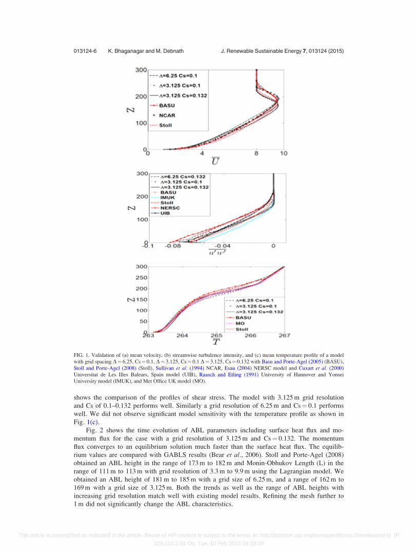
shows the comparison of the profiles of shear stress. The model with 3.125 m grid resolution

and Cs of 0.1–0.132 performs well. Similarly a grid resolution of 6.25 m and Cs¼ 0.1 performs

well. We did not observe significant model sensitivity with the temperature profile as shown in

Fig. 1(c).

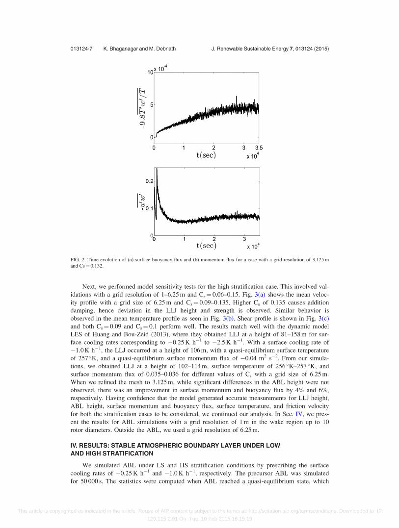
Fig. 2 shows the time evolution of ABL parameters including surface heat flux and mo-

mentum flux for the case with a grid resolution of 3.125 m and Cs¼ 0.132. The momentum

flux converges to an equilibrium solution much faster than the surface heat flux. The equilib-

rium values are compared with GABLS results (Bear et al., 2006). Stoll and Porte-Agel (2008)

obtained an ABL height in the range of 173 m to 182 m and Monin-Obhukov Length (L) in the

range of 111 m to 113 m with grid resolution of 3.3 m to 9.9 m using the Lagrangian model. We

obtained an ABL height of 181 m to 185 m with a grid size of 6.25 m, and a range of 162 m to

169 m with a grid size of 3.125 m. Both the trends as well as the range of ABL heights with

increasing grid resolution match well with existing model results. Refining the mesh further to

1 m did not significantly change the ABL characteristics.

FIG. 1. Validation of (a) mean velocity, (b) streamwise turbulence intensity, and (c) mean temperature profile of a model

with grid spacing D¼ 6.25, Cs¼ 0.1, D¼ 3.125, Cs¼ 0.1 D¼ 3.125, Cs¼ 0.132 with Basu and Porte-Agel (2005) (BASU),

Stoll and Porte-Agel (2008) (Stoll), Sullivan et al. (1994) NCAR, Esau (2004) NERSC model and Cuxart et al. (2000)

Universitat de Les Illes Balears, Spain model (UIB), Raasch and Etling (1991) University of Hannover and Yonsei

University model (IMUK), and Met Office UK model (MO).

013124-6 K. Bhaganagar and M. Debnath J. Renewable Sustainable Energy 7, 013124 (2015)

This article is copyrighted as indicated in the article. Reuse of AIP content is subject to the terms at: http://scitation.aip.org/termsconditions. Downloaded to IP:

129.115.2.91 On: Tue, 10 Feb 2015 16:15:19

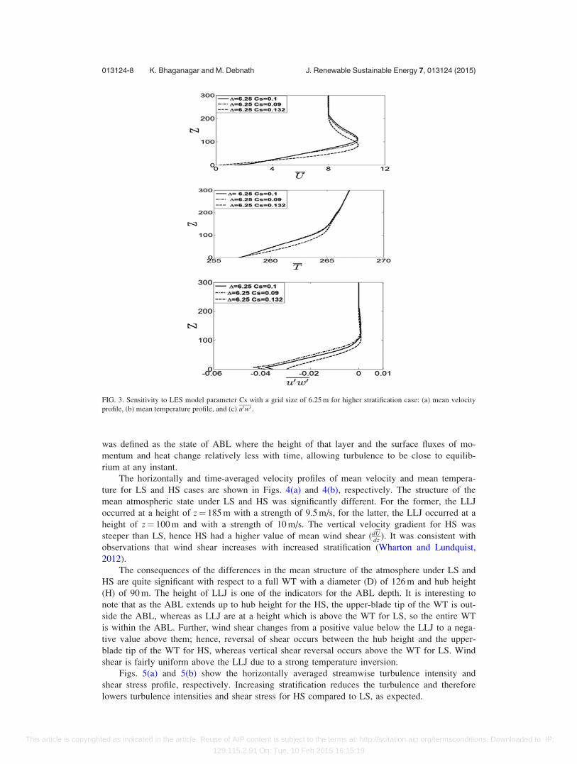
Next, we performed model sensitivity tests for the high stratification case. This involved val-

idations with a grid resolution of 1–6.25 m and Cs¼ 0.06–0.15. Fig. 3(a) shows the mean veloc-

ity profile with a grid size of 6.25 m and Cs¼ 0.09–0.135. Higher Cs of 0.135 causes addition

damping, hence deviation in the LLJ height and strength is observed. Similar behavior is

observed in the mean temperature profile as seen in Fig. 3(b). Shear profile is shown in Fig. 3(c)

and both Cs¼ 0.09 and Cs¼ 0.1 perform well. The results match well with the dynamic model

LES of Huang and Bou-Zeid (2013), where they obtained LLJ at a height of 81–158 m for sur-

face cooling rates corresponding to �0.25 K h�1 to �2.5 K h�1. With a surface cooling rate of

�1.0 K h�1, the LLJ occurred at a height of 106 m, with a quasi-equilibrium surface temperature

of 257 �K, and a quasi-equilibrium surface momentum flux of �0.04 m2 s�2. From our simula-

tions, we obtained LLJ at a height of 102–114 m, surface temperature of 256 �K–257 �K, and

surface momentum flux of 0.035–0.036 for different values of Cs with a grid size of 6.25 m.

When we refined the mesh to 3.125 m, while significant differences in the ABL height were not

observed, there was an improvement in surface momentum and buoyancy flux by 4% and 6%,

respectively. Having confidence that the model generated accurate measurements for LLJ height,

ABL height, surface momentum and buoyancy flux, surface temperature, and friction velocity

for both the stratification cases to be considered, we continued our analysis. In Sec. IV, we pres-

ent the results for ABL simulations with a grid resolution of 1 m in the wake region up to 10

rotor diameters. Outside the ABL, we used a grid resolution of 6.25 m.

IV. RESULTS: STABLE ATMOSPHERIC BOUNDARY LAYER UNDER LOW

AND HIGH STRATIFICATION

We simulated ABL under LS and HS stratification conditions by prescribing the surface

cooling rates of �0.25 K h�1 and �1.0 K h�1, respectively. The precursor ABL was simulated

for 50 000 s. The statistics were computed when ABL reached a quasi-equilibrium state, which

FIG. 2. Time evolution of (a) surface buoyancy flux and (b) momentum flux for a case with a grid resolution of 3.125 m

and Cs¼ 0.132.

013124-7 K. Bhaganagar and M. Debnath J. Renewable Sustainable Energy 7, 013124 (2015)

This article is copyrighted as indicated in the article. Reuse of AIP content is subject to the terms at: http://scitation.aip.org/termsconditions. Downloaded to IP:

129.115.2.91 On: Tue, 10 Feb 2015 16:15:19

was defined as the state of ABL where the height of that layer and the surface fluxes of mo-

mentum and heat change relatively less with time, allowing turbulence to be close to equilib-

rium at any instant.

The horizontally and time-averaged velocity profiles of mean velocity and mean tempera-

ture for LS and HS cases are shown in Figs. 4(a) and 4(b), respectively. The structure of the

mean atmospheric state under LS and HS was significantly different. For the former, the LLJ

occurred at a height of z¼ 185 m with a strength of 9.5 m/s, for the latter, the LLJ occurred at a

height of z¼ 100 m and with a strength of 10 m/s. The vertical velocity gradient for HS was

steeper than LS, hence HS had a higher value of mean wind shear (dUdz ). It was consistent with

observations that wind shear increases with increased stratification (Wharton and Lundquist,

2012).

The consequences of the differences in the mean structure of the atmosphere under LS and

HS are quite significant with respect to a full WT with a diameter (D) of 126 m and hub height

(H) of 90 m. The height of LLJ is one of the indicators for the ABL depth. It is interesting to

note that as the ABL extends up to hub height for the HS, the upper-blade tip of the WT is out-

side the ABL, whereas as LLJ are at a height which is above the WT for LS, so the entire WT

is within the ABL. Further, wind shear changes from a positive value below the LLJ to a nega-

tive value above them; hence, reversal of shear occurs between the hub height and the upper-

blade tip of the WT for HS, whereas vertical shear reversal occurs above the WT for LS. Wind

shear is fairly uniform above the LLJ due to a strong temperature inversion.

Figs. 5(a) and 5(b) show the horizontally averaged streamwise turbulence intensity and

shear stress profile, respectively. Increasing stratification reduces the turbulence and therefore

lowers turbulence intensities and shear stress for HS compared to LS, as expected.

FIG. 3. Sensitivity to LES model parameter Cs with a grid size of 6.25 m for higher stratification case: (a) mean velocity

profile, (b) mean temperature profile, and (c) u0w0 .

013124-8 K. Bhaganagar and M. Debnath J. Renewable Sustainable Energy 7, 013124 (2015)

This article is copyrighted as indicated in the article. Reuse of AIP content is subject to the terms at: http://scitation.aip.org/termsconditions. Downloaded to IP:

129.115.2.91 On: Tue, 10 Feb 2015 16:15:19

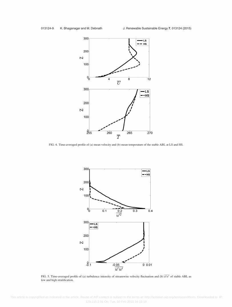
FIG. 4. Time-averaged profile of (a) mean velocity and (b) mean temperature of the stable ABL at LS and HS.

FIG. 5. Time-averaged profile of (a) turbulence intensity of streamwise velocity fluctuation and (b) u0w0 of stable ABL as

low and high stratification.

013124-9 K. Bhaganagar and M. Debnath J. Renewable Sustainable Energy 7, 013124 (2015)

This article is copyrighted as indicated in the article. Reuse of AIP content is subject to the terms at: http://scitation.aip.org/termsconditions. Downloaded to IP:

129.115.2.91 On: Tue, 10 Feb 2015 16:15:19

In Sec. V, we present the results for the wind turbine simulations subjected to mean ABL

forcings. The rotation speed of the turbine has been fixed at 5 rpm. The corresponding tip-

speed-ratio which is ratio of the tangential tip of the tip of the blade and the wind velocity is

4.9 for LS and 3.36 for HS, respectively.

V. RESULTS: WIND TURBINE SUBJECTED TO MEAN ABL FORCINGS

In this section, we discuss the effect of the mean ABL forcings subjected to two different

stratifications (LS and HS) on the wake of WTs in a stable ABL. For this purpose, the precur-

sor ABL simulations were performed to obtain a quasi-equilibrium mean state. We performed

the WT simulations under the same boundary conditions and surface-cooling rate as the ABL.

The simulations were performed with a grid size of 1-m resolutions up to 10-D downstream

from the WT. A resolution of 3.125 m was used in regions away from the wake. The initial

mean velocity and temperature profiles and the surface heat and momentum flux for the WT

simulations were obtained from precursor ABL simulations. The turbulence state generated

from the ABL simulation had peak amplitude close to the surface of 4% of inflow velocity. To

the ABL mean state, we added artificial 3D periodic, homogenous, isotropic turbulence with

4% TKE as inflow conditions, and we performed the simulations for 180 s. The statistics were

averaged in the last 80 s after the initial transience has passed.

We analyzed energetics (balance terms of the TKE transport equation) and turbulence

structures in the WT wake, which together define the turbulence. TKE generated in the wake

region is primarily a balance of the shear production and buoyancy damping. The shear produc-

tion of TKE is the transfer of energy from large-scale to small-scale turbulence and is given as

�u0w0 dUdz . High velocity gradients and high Reynolds stresses lead to higher turbulence produc-

tion. The production from buoyancy term T0w0 dTdz contributes to turbulence damping due to a

negative temperature gradient. In Sec. V A, we present the flow statistics.

The dominant turbulence structures in the wake-region of the WTs are primarily blade tip

and root vortex. Various vortex detection algorithms have evolved to identify vortices in turbu-

lent flows. A pressure minimum is a generally used criterion to detect vortex centers. Having

demonstrated that a pressure minimum might not be a sufficient criterion (as viscous effects

might eliminate pressure minima), Jeong and Hussain (1995) developed the k2 criterion to

extract the dominant vortical structure of the flow. This method defines a vortex as a region

where the second largest eigenvalue of SijSij þ XijXij (Sij and Xij are the symmetric and anti-

symmetric components of the velocity gradient tensor) is negative. In Sec. V B 2, we use the k2

criterion to extract the hub and the tip vortex.

A. Energetics

1. Mean velocity profile and velocity deficit

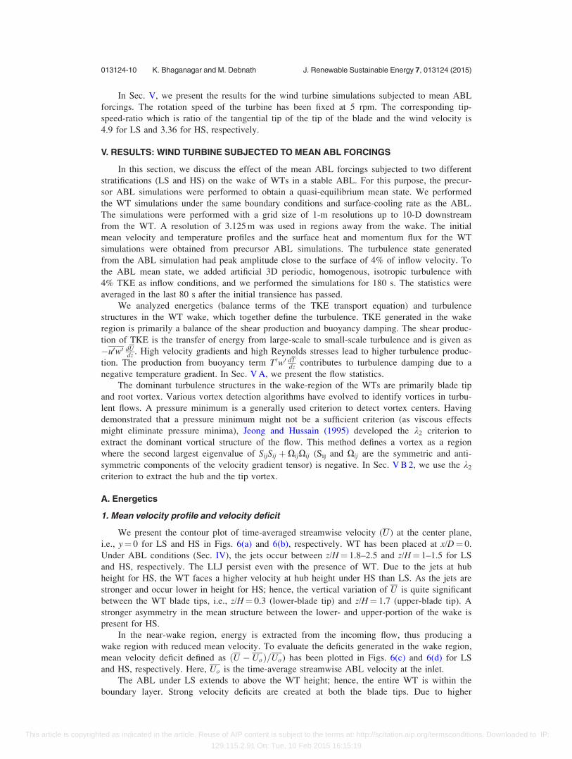
We present the contour plot of time-averaged streamwise velocity (U) at the center plane,

i.e., y¼ 0 for LS and HS in Figs. 6(a) and 6(b), respectively. WT has been placed at x/D¼ 0.

Under ABL conditions (Sec. IV), the jets occur between z/H¼ 1.8–2.5 and z/H¼ 1–1.5 for LS

and HS, respectively. The LLJ persist even with the presence of WT. Due to the jets at hub

height for HS, the WT faces a higher velocity at hub height under HS than LS. As the jets are

stronger and occur lower in height for HS; hence, the vertical variation of U is quite significant

between the WT blade tips, i.e., z/H¼ 0.3 (lower-blade tip) and z/H¼ 1.7 (upper-blade tip). A

stronger asymmetry in the mean structure between the lower- and upper-portion of the wake is

present for HS.

In the near-wake region, energy is extracted from the incoming flow, thus producing a

wake region with reduced mean velocity. To evaluate the deficits generated in the wake region,

mean velocity deficit defined as ðU � UoÞ=Uo ) has been plotted in Figs. 6(c) and 6(d) for LS

and HS, respectively. Here, Uo is the time-average streamwise ABL velocity at the inlet.

The ABL under LS extends to above the WT height; hence, the entire WT is within the

boundary layer. Strong velocity deficits are created at both the blade tips. Due to higher

013124-10 K. Bhaganagar and M. Debnath J. Renewable Sustainable Energy 7, 013124 (2015)

This article is copyrighted as indicated in the article. Reuse of AIP content is subject to the terms at: http://scitation.aip.org/termsconditions. Downloaded to IP:

129.115.2.91 On: Tue, 10 Feb 2015 16:15:19

turbulence and mixing in the ABL, the deficits for LS are between 36% and 40%. On the other

hand, the mixing for HS is confined to the lower-region of the wake (below the hub height) as

the ABL extends slightly above the hub height, resulting in strong asymmetry in the lower and

upper-regions (above the hub height) of the wake. The maximum velocity deficit is 30% for

HS. Due to mixing the wake expands up to 3D and 2D for LS and HS, respectively. The wake

recovery is faster for LS than HS, as expected. Higher the turbulence the faster is the recovery.

At x/D¼ 7, LS has recovered with deficits of less than 8%, whereas the deficits of 12% persist

for LS at this downstream location.

In summary, regions of low momentum fluid are created near the blade tips for the WT in

ABL under LS. Due to mixing and higher turbulence, high velocity deficits are created both in

the lower- and upper-regions of the near-wake region. The wake recovery is fast due to mixing.

On the other hand, for the WT in ABL under HS, asymmetric wake develops with higher

FIG. 6. (a) Time-averaged streamwise velocity for LS, (b) Time-averaged streamwise velocity for HS, (c) Streamwise

mean velocity deficit of LS, and (d) Streamwise mean velocity deficit of HS plotted in the center plane y/D¼ 0.

013124-11 K. Bhaganagar and M. Debnath J. Renewable Sustainable Energy 7, 013124 (2015)

This article is copyrighted as indicated in the article. Reuse of AIP content is subject to the terms at: http://scitation.aip.org/termsconditions. Downloaded to IP:

129.115.2.91 On: Tue, 10 Feb 2015 16:15:19

deficits in the lower-region of the wake. As mixing is confined to region within the ABL, hence

the wake recovery is slower in the upper-region of the wake, which is outside the ABL for HS.

2. Mean shear

Wind shear is the primary source of turbulence in stable stratified ABL. As LS and HS

clearly show differences in the mean velocity deficit, now the question arises as to what the dif-

ferences are in the turbulence generated in the wake region. We next investigate the TKE produc-

tion, turbulence damping, and the TKE generated in the WT wake. For this purpose, shear stress

(u0w0 ), mean shear (dUdz ), TKE production (�u0w0 dU

dz ), mean temperature gradient (dTdz), and TKE

are analyzed.

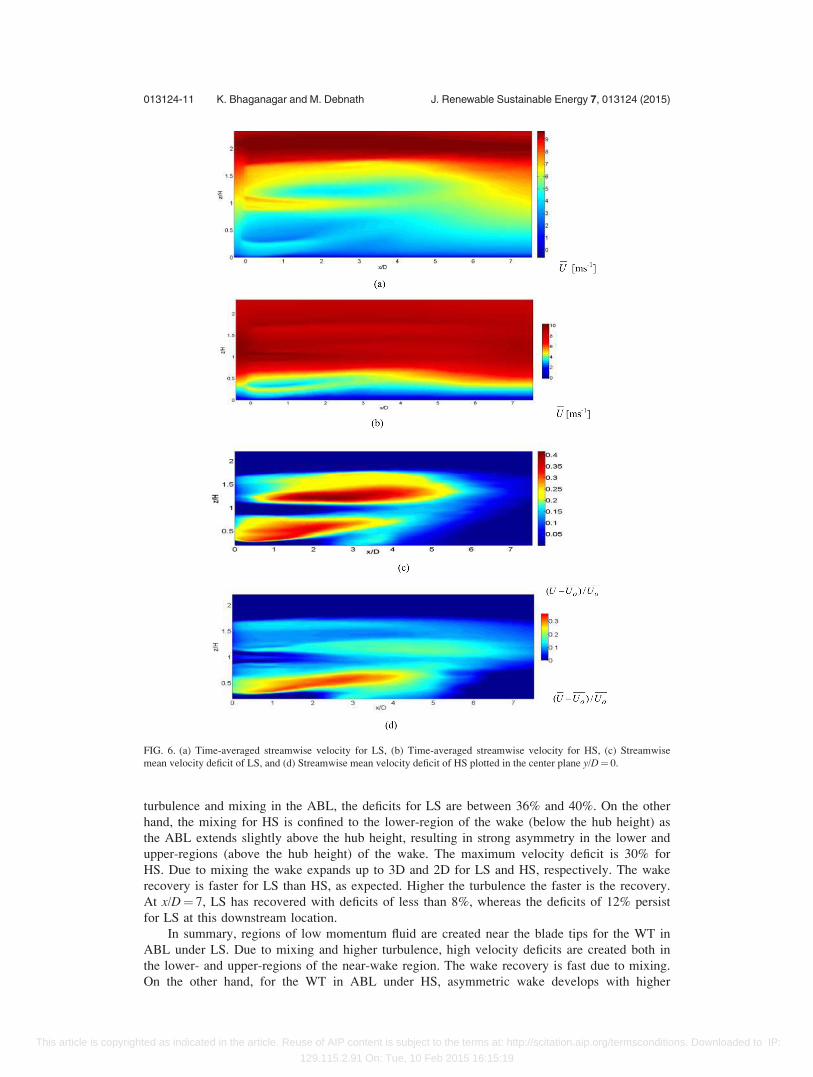
The contours of mean wind shear (dUdz ) are presented in Fig. 7. The wind shear is almost

uniform between the lower- and upper-tips of the blade for LS. Vertical shear reversal occurs

just above the LLJ, which is slightly above the WT. For HS, the shear acting on the lower- and

upper-tip is quite different. The lower-tip of the blade is subjected to high shear and the upper-

tip is outside the ABL. Further, vertical shear reversal occurs within the WT domain as the LLJ

occur near the hub height. Thus, the WT under high stratification is subjected to wind with

non-uniform vertical shear. The significant differences LS and HS are that the vertical shear

acting on the lower-tip is higher for the HS than for the LS in the near-wake region. The verti-

cal shear reversal (i.e., from negative to positive) occurs above the WT for LS and near the

hub height for HS. A negative shear contributes to TKE production, and a positive shear damps

the TKE production, thus suggesting that as shear is higher for the HS, hence shear-induced

damping occurs within the WT wake region.

FIG. 7. Mean vertical shear profile: (a) LS and (b) HS plotted at the center plane y/D¼ 0.

013124-12 K. Bhaganagar and M. Debnath J. Renewable Sustainable Energy 7, 013124 (2015)

This article is copyrighted as indicated in the article. Reuse of AIP content is subject to the terms at: http://scitation.aip.org/termsconditions. Downloaded to IP:

129.115.2.91 On: Tue, 10 Feb 2015 16:15:19

3. Reynolds stress, TKE, turbulence production

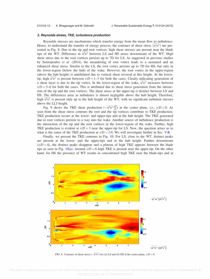
Reynolds stresses are mechanisms which transfer energy from the mean flow to turbulence.

Hence, to understand the transfer of energy process, the contours of shear stress ðu0w0 Þ are pre-

sented in Fig. 8. Due to the tip and root vortices, high shear stresses are present near the blade

tips of the WT. Difference in u0w0 between LS and HS arises downstream of the WT. High

shear stress due to the root vortices persists up to 7D for LS. As suggested in previous studies

by Sotiropoulos et al. (2014), the meandering of root vortex leads to a sustained and an

enhanced shear stress. Similar to the LS, the root vortex persists up to 7D for HS, but only in

the lower-region (below the hub) of the wake. However, the root vortex in the upper-region

(above the hub height) is annihilated due to vertical shear reversal at this height. At the lower-

tip, high u0w0 is present between x/D¼ 1–3 for both the cases. Clearly indicating generation of

a shear layer is due to the tip vortex. In the lower-region of the wake, u0w0 increases between

x/D¼ 3–6 for both the cases. This is attributed due to shear stress generation from the interac-

tion of the tip and the root vortices. The shear stress at the upper-tip is distinct between LS and

HS. The differences arise as turbulence is almost negligible above the hub height. Therefore,

high u0w0 is present only up to the hub height of the WT, with no significant turbulent stresses

above the LLJ height.

Fig. 9 shows the TKE shear production (�u0w0 dUdz ) at the center plane, i.e., y/D¼ 0. As

seen from the shear stress contours the root and the tip vortices contribute to TKE production.

TKE production occurs at the lower- and upper-tips and at the hub height. The TKE generated

due to root vortices persists to a way into the wake. Another source of turbulence production is

the interaction of the tip and the root vortices in the lower-region of the wake. Further, high

TKE production is evident at x/D¼ 3 near the upper-tip for LS. Now, the question arises as to

what is the cause of the TKE production at x/D¼ 3.0. We will investigate further in Sec. V B.

Finally, we present the TKE contours in Fig. 10. For LS, close to the WT, distinct peaks

are present at the lower- and the upper-tips and at the hub height. Further downstream

(x/D¼ 4), the distinct peaks disappear and a plateau of high TKE appears between the blade

tips as seen in Fig. 10(a). Around x/D¼ 6 high TKE is present near the upper-tip. On the other

hand, for HS the presence of WT results in concentrated high TKE near the blade-tips and at

FIG. 8. Contours of shear stress (�u0w0 ) for (a) LS and (b) HS at the center plane, y/D¼ 0.

013124-13 K. Bhaganagar and M. Debnath J. Renewable Sustainable Energy 7, 013124 (2015)

This article is copyrighted as indicated in the article. Reuse of AIP content is subject to the terms at: http://scitation.aip.org/termsconditions. Downloaded to IP:

129.115.2.91 On: Tue, 10 Feb 2015 16:15:19

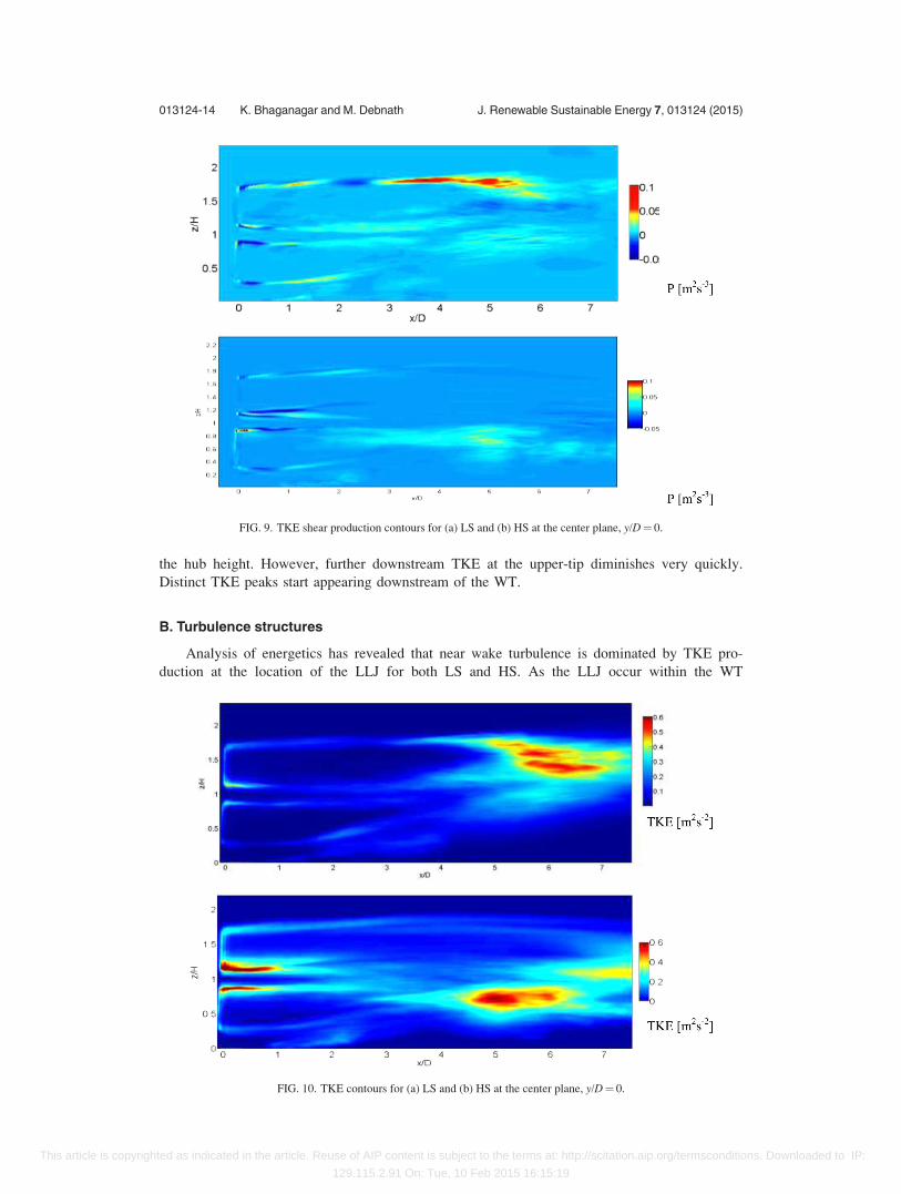
the hub height. However, further downstream TKE at the upper-tip diminishes very quickly.

Distinct TKE peaks start appearing downstream of the WT.

B. Turbulence structures

Analysis of energetics has revealed that near wake turbulence is dominated by TKE pro-

duction at the location of the LLJ for both LS and HS. As the LLJ occur within the WT

FIG. 9. TKE shear production contours for (a) LS and (b) HS at the center plane, y/D¼ 0.

FIG. 10. TKE contours for (a) LS and (b) HS at the center plane, y/D¼ 0.

013124-14 K. Bhaganagar and M. Debnath J. Renewable Sustainable Energy 7, 013124 (2015)

This article is copyrighted as indicated in the article. Reuse of AIP content is subject to the terms at: http://scitation.aip.org/termsconditions. Downloaded to IP:

129.115.2.91 On: Tue, 10 Feb 2015 16:15:19

domain, turbulence mixing is limited and concentrated at the LLJ height for HS. However, for

LS, the TKE is distributed throughout the WT height. Next, we focus on the nature of the tur-

bulent structures to complete the picture obtained from the energetics.

1. Velocity structures

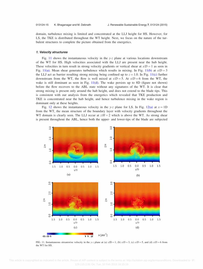
Fig. 11 shows the instantaneous velocity in the y-z plane at various locations downstream

of the WT for HS. High velocities associated with the LLJ are present near the hub height.

These velocities in turn result in strong velocity gradients or vertical shear at x/D¼ 1 as seen in

Fig. 11(a). Mean shear generates turbulence which results in mixing. In Fig. 11(b) at x/D¼ 3

the LLJ act as barrier resulting strong mixing being confined up to z¼ 1.0. In Fig. 11(c) further

downstream from the WT, the flow is well mixed at x/D¼ 5. At x/D¼ 6 from the WT, the

wake is still dominant as seen in Fig. 11(d). The wake persists up to 8D (figure not shown)

before the flow recovers to the ABL state without any signatures of the WT. It is clear that

strong mixing is present only around the hub height, and does not extend to the blade tips. This

is consistent with our analysis from the energetics which revealed that TKE production and

TKE is concentrated near the hub height, and hence turbulence mixing in the wake region is

dominant only at these heights.

Fig. 12 shows the instantaneous velocity in the y-z plane for LS. In Fig. 12(a) at x¼ 1D

from the WT, the mean structure of the boundary layer with velocity gradients throughout the

WT domain is clearly seen. The LLJ occur at z/H¼ 2 which is above the WT. As strong shear

is present throughout the ABL, hence both the upper- and lower-tips of the blade are subjected

FIG. 11. Instantaneous streamwise velocity in the y-z plane at (a) x/D¼ 1, (b) x/D¼ 3, (c) x/D¼ 5, and (d) x/D¼ 6 from

the WT for HS.

013124-15 K. Bhaganagar and M. Debnath J. Renewable Sustainable Energy 7, 013124 (2015)

This article is copyrighted as indicated in the article. Reuse of AIP content is subject to the terms at: http://scitation.aip.org/termsconditions. Downloaded to IP:

129.115.2.91 On: Tue, 10 Feb 2015 16:15:19

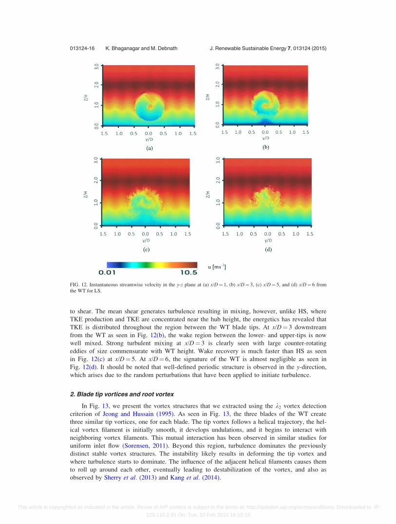
to shear. The mean shear generates turbulence resulting in mixing, however, unlike HS, where

TKE production and TKE are concentrated near the hub height, the energetics has revealed that

TKE is distributed throughout the region between the WT blade tips. At x/D¼ 3 downstream

from the WT as seen in Fig. 12(b), the wake region between the lower- and upper-tips is now

well mixed. Strong turbulent mixing at x/D¼ 3 is clearly seen with large counter-rotating

eddies of size commensurate with WT height. Wake recovery is much faster than HS as seen

in Fig. 12(c) at x/D¼ 5. At x/D¼ 6, the signature of the WT is almost negligible as seen in

Fig. 12(d). It should be noted that well-defined periodic structure is observed in the y-direction,

which arises due to the random perturbations that have been applied to initiate turbulence.

2. Blade tip vortices and root vortex

In Fig. 13, we present the vortex structures that we extracted using the k2 vortex detection

criterion of Jeong and Hussain (1995). As seen in Fig. 13, the three blades of the WT create

three similar tip vortices, one for each blade. The tip vortex follows a helical trajectory, the hel-

ical vortex filament is initially smooth, it develops undulations, and it begins to interact with

neighboring vortex filaments. This mutual interaction has been observed in similar studies for

uniform inlet flow (Sorensen, 2011). Beyond this region, turbulence dominates the previously

distinct stable vortex structures. The instability likely results in deforming the tip vortex and

where turbulence starts to dominate. The influence of the adjacent helical filaments causes them

to roll up around each other, eventually leading to destabilization of the vortex, and also as

observed by Sherry et al. (2013) and Kang et al. (2014).

FIG. 12. Instantaneous streamwise velocity in the y-z plane at (a) x/D¼ 1, (b) x/D¼ 3, (c) x/D¼ 5, and (d) x/D¼ 6 from

the WT for LS.

013124-16 K. Bhaganagar and M. Debnath J. Renewable Sustainable Energy 7, 013124 (2015)

This article is copyrighted as indicated in the article. Reuse of AIP content is subject to the terms at: http://scitation.aip.org/termsconditions. Downloaded to IP:

129.115.2.91 On: Tue, 10 Feb 2015 16:15:19

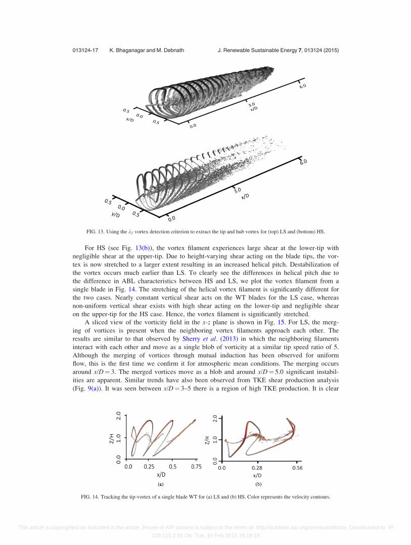
For HS (see Fig. 13(b)), the vortex filament experiences large shear at the lower-tip with

negligible shear at the upper-tip. Due to height-varying shear acting on the blade tips, the vor-

tex is now stretched to a larger extent resulting in an increased helical pitch. Destabilization of

the vortex occurs much earlier than LS. To clearly see the differences in helical pitch due to

the difference in ABL characteristics between HS and LS, we plot the vortex filament from a

single blade in Fig. 14. The stretching of the helical vortex filament is significantly different for

the two cases. Nearly constant vertical shear acts on the WT blades for the LS case, whereas

non-uniform vertical shear exists with high shear acting on the lower-tip and negligible shear

on the upper-tip for the HS case. Hence, the vortex filament is significantly stretched.

A sliced view of the vorticity field in the x-z plane is shown in Fig. 15. For LS, the merg-

ing of vortices is present when the neighboring vortex filaments approach each other. The

results are similar to that observed by Sherry et al. (2013) in which the neighboring filaments

interact with each other and move as a single blob of vorticity at a similar tip speed ratio of 5.

Although the merging of vortices through mutual induction has been observed for uniform

flow, this is the first time we confirm it for atmospheric mean conditions. The merging occurs

around x/D¼ 3. The merged vortices move as a blob and around x/D¼ 5.0 significant instabil-

ities are apparent. Similar trends have also been observed from TKE shear production analysis

(Fig. 9(a)). It was seen between x/D¼ 3–5 there is a region of high TKE production. It is clear

FIG. 13. Using the k2 vortex detection criterion to extract the tip and hub vortex for (top) LS and (bottom) HS.

FIG. 14. Tracking the tip-vortex of a single blade WT for (a) LS and (b) HS. Color represents the velocity contours.

013124-17 K. Bhaganagar and M. Debnath J. Renewable Sustainable Energy 7, 013124 (2015)

This article is copyrighted as indicated in the article. Reuse of AIP content is subject to the terms at: http://scitation.aip.org/termsconditions. Downloaded to IP:

129.115.2.91 On: Tue, 10 Feb 2015 16:15:19

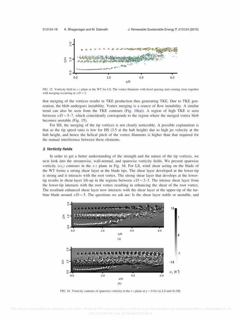
that merging of the vortices results in TKE production thus generating TKE. Due to TKE gen-

eration, the blob undergoes instability. Vortex merging is a source of flow instability. A similar

trend can also be seen from the TKE contours (Fig. 10(a)). A region of high TKE is seen

between x/D¼ 5–7, which coincidently corresponds to the region where the merged vortex blob

becomes unstable (Fig. 15).

For HS, the merging of the tip vortices is not clearly noticeable. A possible explanation is

that as the tip speed ratio is low for HS (3.5 at the hub height) due to high jet velocity at the

hub height, and hence the helical pitch of the vortex filaments is higher than that required for

the mutual interference between these elements.

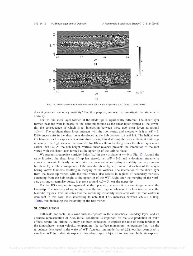
3. Vorticity fields

In order to get a better understanding of the strength and the nature of the tip vortices, we

next look into the streamwise, wall-normal, and spanwise vorticity fields. We present spanwise

vorticity (xy) contours in the x-z plane in Fig. 16. For LS, wind shear acting on the blade of

the WT forms a strong shear layer at the blade tips. The shear layer developed at the lower-tip

is strong and it interacts with the root vortex. The strong shear layer that develops at the lower-

tip results in shear-layer lift-up in the regions between x/D¼ 2–3. The intense shear layer from

the lower-tip interacts with the root vortex resulting in enhancing the shear of the root vortex.

The resultant enhanced shear layer now interacts with the shear layer at the upper-tip of the tur-

bine blade around x/D¼ 5. The questions we ask are: Is the shear layer stable or unstable, and

FIG. 15. Vorticity field in x-z plane at the WT for LS. The vortex filaments with fixed spacing start coming close together

with merging occurring at x/D¼ 3.

FIG. 16. Vorticity contours of spanwise vorticity in the x-z plane at y¼ 0 for (a) LS and (b) HS.

013124-18 K. Bhaganagar and M. Debnath J. Renewable Sustainable Energy 7, 013124 (2015)

This article is copyrighted as indicated in the article. Reuse of AIP content is subject to the terms at: http://scitation.aip.org/termsconditions. Downloaded to IP:

129.115.2.91 On: Tue, 10 Feb 2015 16:15:19

does it generate secondary vorticity? For this purpose, we need to investigate the streamwise

vorticity.

For HS, the shear layer formed at the blade tips is significantly different. The shear layer

formed near the wall is nearly of the same magnitude as the shear layer formed at the lower-

tip, the consequence of which is an interaction between these two shear layers at around

x/D¼ 1. The resultant shear layer interacts with the root vortex and merges with it at x/D¼ 3.

Differences exist in the shear layer developed at the hub between LS and HS. The helical vor-

tex filament for HS experiences non-uniform shear, thus distorting the vortex filament quite sig-

nificantly. The high shear at the lower-tip for HS results in breaking down the shear layer much

earlier than LS. At the hub height, vertical shear reversal prevents the interaction of the root

vortex with the shear layer formed at the upper-tip of the turbine blade.

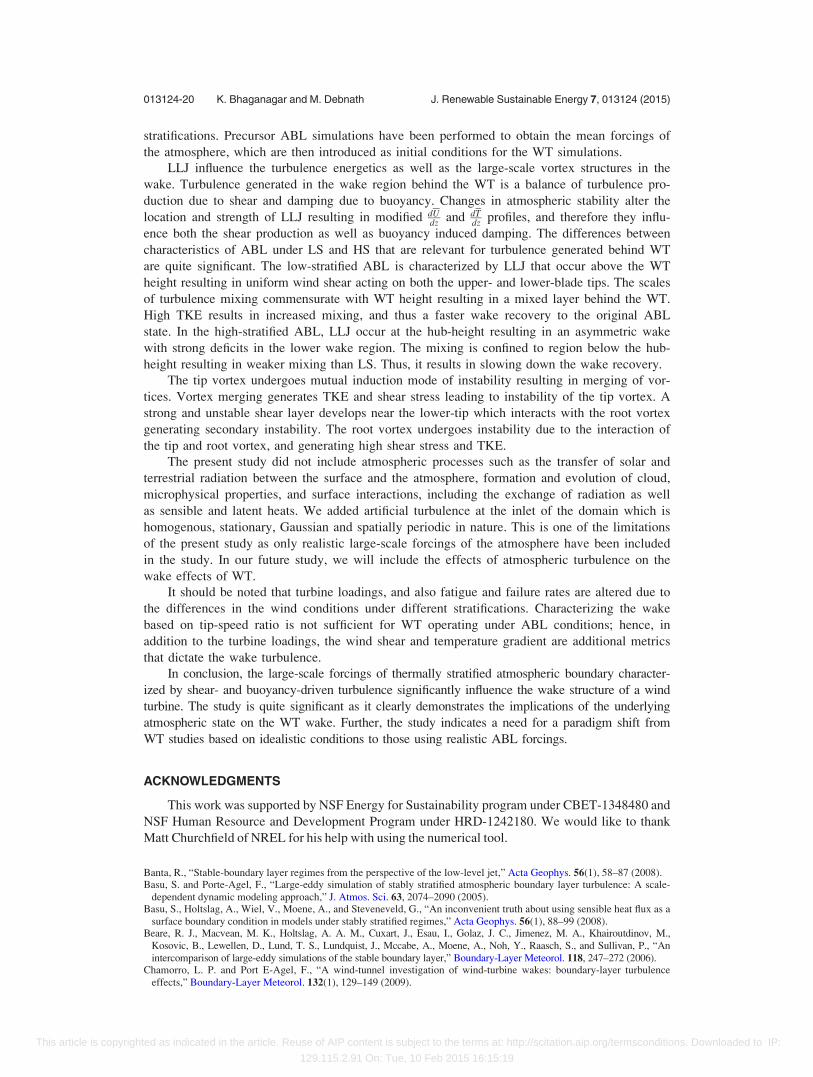
We present streamwise vorticity fields (xx) in the x-z plane at y¼ 0 in Fig. 17. Around the

same location, the shear layer lift-up has started, i.e., x/D¼ 2–3, and a dominant streamwise

vortex is present. It clearly demonstrates the presence of secondary instability due to an unsta-

ble shear layer. The consequence of the unstable shear layer is mutual interaction of the neigh-

boring vortex filaments resulting in merging of the vortices. The interaction of the shear layer

from the lower-tip vortex with the root vortex also results in regions of secondary vorticity

extending from the hub height to the upper-tip of the WT. Right after the merging of the vorti-

ces, a strong streamwise vortex is present around x/D¼ 5 near the upper-tip.

For the HS case, xx is organized at the upper-tip, whereas it is more irregular near the

lower-tip. The intensity of xx is high near the hub region, whereas it is less intense near the

blade-tip regions. This indicates that the secondary instability associated with the root vortex is

dominant in this case. It is interesting to note that TKE increases between x/D¼ 4–6 (Fig.

10(b)), thus indicating the instability of the root vortex.

VI. CONCLUSION

Full-scale horizontal axis wind turbines operate in the atmospheric boundary layer, and an

accurate representation of ABL initial conditions is important for realistic prediction of wake

effects behind the turbine. A study has been conducted to explore the role of mean forcings of

the atmosphere—mean velocity, temperature, the surface momentum, temperature-flux—on the

turbulence developed in the wake of WT. Actuator line model based LES tool has been used to

simulate WT in stable atmospheric boundary layer subjected to low and high atmospheric

FIG. 17. Vorticity contours of streamwise vorticity in the x-z plane at y¼ 0 for (a) LS and (b) HS.

013124-19 K. Bhaganagar and M. Debnath J. Renewable Sustainable Energy 7, 013124 (2015)

This article is copyrighted as indicated in the article. Reuse of AIP content is subject to the terms at: http://scitation.aip.org/termsconditions. Downloaded to IP:

129.115.2.91 On: Tue, 10 Feb 2015 16:15:19

stratifications. Precursor ABL simulations have been performed to obtain the mean forcings of

the atmosphere, which are then introduced as initial conditions for the WT simulations.

LLJ influence the turbulence energetics as well as the large-scale vortex structures in the

wake. Turbulence generated in the wake region behind the WT is a balance of turbulence pro-

duction due to shear and damping due to buoyancy. Changes in atmospheric stability alter the

location and strength of LLJ resulting in modified dUdz and dT

dz profiles, and therefore they influ-

ence both the shear production as well as buoyancy induced damping. The differences between

characteristics of ABL under LS and HS that are relevant for turbulence generated behind WT

are quite significant. The low-stratified ABL is characterized by LLJ that occur above the WT

height resulting in uniform wind shear acting on both the upper- and lower-blade tips. The scales

of turbulence mixing commensurate with WT height resulting in a mixed layer behind the WT.

High TKE results in increased mixing, and thus a faster wake recovery to the original ABL

state. In the high-stratified ABL, LLJ occur at the hub-height resulting in an asymmetric wake

with strong deficits in the lower wake region. The mixing is confined to region below the hub-

height resulting in weaker mixing than LS. Thus, it results in slowing down the wake recovery.

The tip vortex undergoes mutual induction mode of instability resulting in merging of vor-

tices. Vortex merging generates TKE and shear stress leading to instability of the tip vortex. A

strong and unstable shear layer develops near the lower-tip which interacts with the root vortex

generating secondary instability. The root vortex undergoes instability due to the interaction of

the tip and root vortex, and generating high shear stress and TKE.

The present study did not include atmospheric processes such as the transfer of solar and

terrestrial radiation between the surface and the atmosphere, formation and evolution of cloud,

microphysical properties, and surface interactions, including the exchange of radiation as well

as sensible and latent heats. We added artificial turbulence at the inlet of the domain which is

homogenous, stationary, Gaussian and spatially periodic in nature. This is one of the limitations

of the present study as only realistic large-scale forcings of the atmosphere have been included

in the study. In our future study, we will include the effects of atmospheric turbulence on the

wake effects of WT.

It should be noted that turbine loadings, and also fatigue and failure rates are altered due to

the differences in the wind conditions under different stratifications. Characterizing the wake

based on tip-speed ratio is not sufficient for WT operating under ABL conditions; hence, in

addition to the turbine loadings, the wind shear and temperature gradient are additional metrics

that dictate the wake turbulence.

In conclusion, the large-scale forcings of thermally stratified atmospheric boundary character-

ized by shear- and buoyancy-driven turbulence significantly influence the wake structure of a wind

turbine. The study is quite significant as it clearly demonstrates the implications of the underlying

atmospheric state on the WT wake. Further, the study indicates a need for a paradigm shift from

WT studies based on idealistic conditions to those using realistic ABL forcings.

ACKNOWLEDGMENTS

This work was supported by NSF Energy for Sustainability program under CBET-1348480 and

NSF Human Resource and Development Program under HRD-1242180. We would like to thank

Matt Churchfield of NREL for his help with using the numerical tool.

Banta, R., “Stable-boundary layer regimes from the perspective of the low-level jet,” Acta Geophys. 56(1), 58–87 (2008).Basu, S. and Porte-Agel, F., “Large-eddy simulation of stably stratified atmospheric boundary layer turbulence: A scale-

dependent dynamic modeling approach,” J. Atmos. Sci. 63, 2074–2090 (2005).Basu, S., Holtslag, A., Wiel, V., Moene, A., and Steveneveld, G., “An inconvenient truth about using sensible heat flux as a

surface boundary condition in models under stably stratified regimes,” Acta Geophys. 56(1), 88–99 (2008).Beare, R. J., Macvean, M. K., Holtslag, A. A. M., Cuxart, J., Esau, I., Golaz, J. C., Jimenez, M. A., Khairoutdinov, M.,

Kosovic, B., Lewellen, D., Lund, T. S., Lundquist, J., Mccabe, A., Moene, A., Noh, Y., Raasch, S., and Sullivan, P., “Anintercomparison of large-eddy simulations of the stable boundary layer,” Boundary-Layer Meteorol. 118, 247–272 (2006).

Chamorro, L. P. and Port E-Agel, F., “A wind-tunnel investigation of wind-turbine wakes: boundary-layer turbulenceeffects,” Boundary-Layer Meteorol. 132(1), 129–149 (2009).

013124-20 K. Bhaganagar and M. Debnath J. Renewable Sustainable Energy 7, 013124 (2015)

This article is copyrighted as indicated in the article. Reuse of AIP content is subject to the terms at: http://scitation.aip.org/termsconditions. Downloaded to IP:

129.115.2.91 On: Tue, 10 Feb 2015 16:15:19

Churchfield, M., Lee, S., and Moriarty, P., “Adding complex terrain adding complex terrain and stable atmospheric condi-tion capability to the OpenFOAM- based flow solver of the simulator for on/offshore wind farm applications (SOWFA),”paper presented at the 1st Symposium on OpenFoam in Wind Energy Oldenburg, Germany, March 20–21 (2013).

Churchfield, M. J., Li, Y., and Moriarty, P. J., “A large eddy simulation study of wake propagation and power productionin an array of tidal-current turbines,” in 9th European Wave and Tidal Energy Conference, September 4–9, Southampton,England (2011), Paper No. NREL/CP-5000-51765.

Cuxart, J., Bougeault, P., and Redelsperger, J. L., “A turbulence scheme allowing for mesoscale and large-eddy simu-lations,” Q. J. R. Meteorol. Soc. 126, 1–30 (2000).

Esau, I., “Simulation of Ekman boundary layers by large Eddy model with dynamic mixed subfilter closure,” J. Environ.Fluid Mech. 4(3), 273–303 (2004).

Felli, M., Camussi, R., and Di Felice, F., “Mechanisms of evolution of the propeller wake in the transition and far fields,”J. Fluid Mech. 682, 5–53 (2011).

Hu, H., Yang, Z., and Sarkar, P., “Dynamic wind loads and wake characteristics of a wind turbine model in an atmosphericboundary layer wind,” Exp. Fluids 52, 1277–1294 (2012).

Huang, J. and Bou-Zeid, E., “Turbulence and vertical fluxes in the stable atmospheric boundary layer Part I: A large-eddysimulation study,” J. Atmos. Sci. 70(6), 1513–1527 (2013).

Ivanell, S., Mikkelsen, R., Sorensen, J. N., and Henningson, D., “Stability analysis of the tip vortices of a wind turbine,”Wind Energy 13, 705–715 (2010).

Jeong, J. and Hussain, F., “On the identification of a vortex,” J. Fluid Mech. 285, 69–94 (1995).Jha, P., Churchfield, M. J., Moriarty, P. J., and Schmitz, S., “Guidelines for actuator line modeling of wind turbines on

large-Eddy simulation-type grids,” ASME J. Solar Energy Eng. 136, 031003 (2014).Kang, S., Yang, X., and Sotiropoulos, F., “On the onset of wake meandering for an axial flow turbine in a turbulent open

channel flow,” J. Fluid Mech. 744, 376–403 (2014).Khairoutdinov, M. F. and Randall, D. A., “Cloud resolving modeling of the ARM summer 1997: Model formulation,

results, uncertainties, and sensitivities,” J. Atmos. Sci. 60, 607–625 (2003).Kosovic, B. and Curry, J. A., “A large-Eddy simulation study of a quasi-steady stably-stratified atmospheric boundary

layer,” J. Atmos. Sci. 57, 1052–1068 (2000).Lewellen, D. C. and Lewellen, W. S., “Large-Eddy boundary layer entrainment,” J. Atmos. Sci. 55, 2645–2665 (1998).Lilly, D. K., “The representation of small-scale turbulence in numerical simulation experiments,” in Proceedings of IBM

Scientific Computing Symposium on Environmental Sciences, White Plains, NY, IBM Data Process. Div. (1967).Lu, H. and Porte-Agel, F., “Large-Eddy simulation of a very large wind farm in a stable atmospheric boundary layer,”

Phys. Fluids 23, 065101 (2011).Massouh, F. and Dobrev, I., “Exploration of the vortex wake behind of wind turbine rotor,” J. Phys.: Conf. Ser. 75, 012036

(2007).Mirocha, J., Kosovic, B., Aitken, M., and Lundquist, J., “Implementation of a generalized actuator disk wind turbine model

into the weather research and forecasting model for large-eddy simulation applications,” J. Renewable SustainableEnergy 6, 013104 (2014).

Nieuwstadt, F. T. M., “The turbulent structure of the stable, nocturnal boundary layer,” J. Atmos. Sci. 41(14), 2202–2216 (1984).Ohya, Y., Neff, D., and Meroney, R., “Turbulence structure in a stratified boundary layer under stable conditions,”

Boundary-Layer Meteorol. 83, 139–161 (1997).Okulov, V. L. and Sørensen, J. N., “Stability of helical tip vortices in a rotor far wake,” J. Fluid Mech. 576, 1–25 (2007).Poulos, G. S., Blumen, W., Fritts, D. C., Lundquist, J. K., Sun, J., Burns, S. P., and Jensen, M., “CASES-99: A comprehen-

sive investigation of the stable nocturnal boundary layer,” Bull. Am. Meteorol. Soc. 83(4), 555 (2002).Raasch, S. and Etling, D., “Numerical simulations of rotating turbulent thermal convection,” Phys. Atmos. 64, 185–199 (1991).Sherry, M., Nemes, A., Jacono, D. L., Blackburn, H., and Sheridan, J., “The interaction of helical tip and root vortices in a

wind turbine wake,” Phys. Fluids 25(11), 117102 (2013).Sorensen, J. N., “Instability of helical tip vortices in rotor wakes,” J. Fluid Mech. 682, 1–4 (2011).Sørensen, J. N. and Shen, W. Z., “Numerical modeling of wind turbine wakes,” J. Fluids Eng. 124, 393–399 (2002).Stoll, R. and Porte-Agel, F., “Large-eddy simulation of the stable atmospheric boundary layer using dynamic models with

different averaging schemes,” Boundary-Layer Meteorol. 126, 1–28 (2008).Sullivan, P. P., McWilliams, J. C., and Moeng, C.-H., “A subgrid-scale model for large-Eddy simulation of planetary

boundary-layer flows,” Boundary-Layer Meteorol. 71, 247–276 (1994).Troldborg, N., Larsen, G. C., Madsen, H. A., Hansen, K. S., Sørensen, J. N., and Mikkelsen, R., “Numerical simulations of

wake interactions between two wind turbines at various inflow conditions,” Wind Energy 13, 86 (2010).Troldborg, N., Sørensen, J. N., and Mikkelsen, R., “Actuator line simulation of wake of wind turbine operating in turbulent

inflow,” J. Phys.: Conf. Ser. 75, 012063 (2007).Vermeer, L. J., Sorensen, J. N., and Crespo, A., “Wind turbine wake aerodynamics,” Prog. Aerosp. Sci. 39, 467–510

(2003).Whale, J., Papadopoulos, K. H., Anderson, C. G., and Skyner, D. J., “A study of the near wake structure of a wind turbine

comparing measurements from laboratory and full-scale experiments,” Solar Energy 56(6), 621–633 (1996).Wharton, S. and Lundquist, J., “Atmospheric stability effects wind turbine power collection,” Environ. Res. Lett. 7, 014005

(2012).Widnall, S. E., “The stability of a helical vortex filament,” J. Fluid Mech. 54(4), 641–663 (1972).Yang, Z., Sarkar, P., and Hu, H., “Visualization of the tip vortices in a wind turbine wake,” J. Visualization 15(1), 39–44

(2012).Zahle, F. and Sørensen, J., “On the influence of far-wake resolution on wind turbine flow simulations,” J. Phys.: Conf. Ser.

75, 012042 (2007).Zhang, W., Markfort, C. D., and Porte E-Agel, F., “Near-wake flow structure downwind of a wind turbine in a turbulent

boundary layer,” Exp. Fluids 52(5), 1219–1235 (2012).Zhou, B. and Chow, F., “Turbulence modeling for the stable atmospheric boundary layer and implications for wind ener-

gy,” Flow Turbul. Combust. 88, 255–277 (2012).

013124-21 K. Bhaganagar and M. Debnath J. Renewable Sustainable Energy 7, 013124 (2015)

This article is copyrighted as indicated in the article. Reuse of AIP content is subject to the terms at: http://scitation.aip.org/termsconditions. Downloaded to IP:

129.115.2.91 On: Tue, 10 Feb 2015 16:15:19