A Modified PSO Based Solution Approach for Economic Ordered Quantity Problem with Deteriorating Inventory, Time Dependent Demand Considering Order Size Limits, Stock Limits and Prohibited

International Refereed Journal of Engineering and Science (IRJES)

ISSN (Online) 2319-183X, (Print) 2319-1821

Volume 4, Issue 2 (February 2015), PP.63-74

www.irjes.com 63 | Page

A Modified PSO Based Solution Approach for Economic Ordered

Quantity Problem with Deteriorating Inventory, Time Dependent

Demand Considering Order Size Limits, Stock Limits and

Prohibited Ordering Segments

1Ashutosh Khare,

2Dr. B.B. Singh,

3Shalini khare

1(Department of Mathematics, SMS Govt. Science College, Gwalior, India

2(Department of Computer Science Govt. K.R.G. College, Gwalior, India)

3(Department of Electronics, Govt. polytechnic College, Sagar, India

Abstract:- This paper presents formulation of Economic Ordered Quantity (EOQ) problem considering Order

Size Limits, Stock Limits and Prohibited Ordering Segments, after that a modified PSO algorithm that utilizes

the PSO with double chaotic maps is presented to solve this problem. In proposed approach, the logistic map

and lozi map are applied alternatively to the velocity updating function of the particles. Using PSO with

irregular velocity updates which is performed by these maps forces the particles to search greater space for best

global solution. However the random function itself derived from a well-defined mathematical expression which

limits its redundancy hence in the paper we are utilizing the two different chaotic maps which are used

alternatively this mathematically increased the randomness of the function. The simulation of the algorithm for

the formulated EOQ problem verifies the effectiveness and superiority of the algorithm over standard

algorithms for such a complex problem which are difficult to solve by analytical approaches.

Keywords:- Economic Ordered Quantity (EOQ) problem, PSO, Chaotic Maps, Logistic Map, Lozi Map.

I. INTRODUCTION The Economic Ordered Quantity (EOQ) in inventory framework is the key part of inventory systems

and considered as a significant important part of inventory systems. The EOQ issue is considered as

optimization issue in which minimization of the aggregate inventory holding expenses and requesting expenses

is situated as principle goal which ought to be found inside the equality and inequality constraints (operational

compels) limitations. The operational requirements are alluded as maximum inventory level restrictions, change

in every unit expense relying on request size, accumulating rate points of confinement, and deterioration losses

are considered for reasonable operation. Additionally the base requested amount impacts might likewise be

considered. These contemplations make the EOQ issue a vast scale very non-direct compelled streamlining

issue. An alternate viewpoint other than expense which compels to utilize the EOQ is the new stockpiling

approaches and regulations which governs the inventory managers to consider the environmental effects of the

operation. Under these circumstances, requested inventory is not just governed by the unit's capacity of

minimizing the total inventory holding costs and ordering cost, but also their capability of satisfying the

governing policies requirements. In this paper the EOQ problem under the constrains for order size limits, stock

limits and prohibited ordering segments is discussed and then after applied to the EOQ inventory mathematical

model for deteriorating items with exponentially decreasing demand. Finally the objective function for the

combined model is derived to use with PSO algorithm. The rest of the paper is arranged as second segment

shows a concise audit of the related works, the third and fourth section talks about the issue definition and

mathematical modeling, while fifth section clarifies the PSO and the variations utilized followed by and sixth

sections which presents a brief review of chaotic maps, at last in section seventh and eight separately exhibits

the simulated results and conclusion.

II. LITERATURE REVIEW This section discusses some of the recent literatures related to the EOQ problem, inventory modeling

and particle swarm optimization techniques. Liang Yuh Ouyang et al. [1] presented an EOQ inventory

mathematical model for deteriorating items with exponentially decreasing demand. Their model also handles the

shortages and variable rate partial backordering which dependents on the waiting time for the next

replenishment. Kuo-Lung Hou et al. [10] presents an inventory model for deteriorating items considering the

stock-dependent selling rate under inflation and time value of money over a finite planning horizon. The model

allows shortages and partially backlogging at exponential rate. Lianxia Zhao [7] studied an inventory model

with trapezoidal type demand rate and partially backlogging for Weibull-distributed deterioration items and

A Modified PSO Based Solution Approach for Economic Ordered Quantity Problem with …


derived an optimal inventory replenishment policy. Kai-Wayne Chuang et al. [2] studied pricing strategies in

marketing, with objective to find the optimal inventory and pricing strategies for maximizing the net present

value of total profit over the infinite horizon. The studied two variants of models: one without considering

shortage, and the other with shortage. Jonas C.P. Yu [4] developed a deteriorating inventory system with only

one supplier and one buyer. The system considers the collaboration and trade credit between supplier and buyer.

The objective is to maximize the total profit of the whole system when shortage is completely backordered. The

literature also discuss the negotiation mechanism between supplier and buyer in case of shortages and payment

delay. Michal Pluhacek et al [15] compared the performance of two popular evolutionary computational

techniques (particle swarm optimization and differential evolution) is compared in the task of batch reactor

geometry optimization. Both algorithms are enhanced with chaotic pseudo-random number generator

(CPRNG) based on Lozi chaotic map. The application of Chaos Embedded Particle Swarm Optimization for

PID Parameter Tuning is presented in [16]. Magnus Erik et al [17] gives a list of good choices of parameters for

various optimization scenarios which should help the practitioner achieve better results with little effort.

III. PROBLEM FORMULATION The objective of an EOQ problem is to minimize the total inventory holding costs and ordering costs

which should be found within the equality and inequality constraints (operational constrains) limitations. The

simplified cost function of each inventory item can be represented as described in (2)

𝐶𝑇 = 𝑐𝑖(𝑆𝑖)

𝑛

𝑖=1

………………… . . (3.1)

𝑐𝑖 𝑆𝑖 = 𝛼𝑖 ∗ 𝑆𝑖 …… . . . (3.2)

𝑤𝑕𝑒𝑟𝑒 𝐶𝑇 = 𝑇𝑜𝑡𝑎𝑙 𝐼𝑛𝑣𝑒𝑛𝑡𝑜𝑟𝑦 𝐶𝑜𝑠𝑡

𝑐𝑖 = 𝐶𝑜𝑠𝑡 𝐹𝑢𝑛𝑐𝑡𝑖𝑜𝑛 𝑜𝑓 𝐼𝑛𝑣𝑒𝑟𝑡𝑜𝑟𝑦 𝑖 𝛼𝑖 = 𝑝𝑒𝑟 𝑢𝑛𝑖𝑡 𝑐𝑜𝑠𝑡 𝑜𝑓 𝐼𝑛𝑣𝑒𝑟𝑡𝑜𝑟𝑦 𝑖 𝑆𝑖 = 𝑂𝑟𝑑𝑒𝑟𝑒𝑑 𝑠𝑖𝑧𝑒 𝑜𝑓 𝐼𝑛𝑣𝑒𝑟𝑡𝑜𝑟𝑦 𝑖

3.2. Equality and Inequality Constraints

3.2.1 Demand and Stock Balance Equation: For Demand and Stock balance, an equality constraint should be

satisfied. The total stock should be equal or greater than the total demand plus the total Deterioration loss

𝑆𝑖 ,𝑑𝑒𝑚𝑎𝑛𝑑 + 𝑆𝑖 ,𝑙𝑜𝑠𝑠 ………… . . (3.14)

𝑛

𝑖=1

𝑤𝑕𝑒𝑟𝑒 𝑆𝑖 ,𝑑𝑒𝑚𝑎𝑛𝑑 𝑆𝑖 ,𝑙𝑜𝑠𝑠 𝑟𝑒𝑝𝑟𝑒𝑠𝑒𝑛𝑡𝑠 𝑡𝑕𝑒 𝑡𝑜𝑡𝑎𝑙 𝑑𝑒𝑚𝑎𝑛𝑑 𝑎𝑛𝑑

𝐷𝑒𝑡𝑒𝑟𝑖𝑜𝑟𝑎𝑡𝑖𝑜𝑛 𝑙𝑜𝑠𝑠 𝑜𝑓 𝑖𝑡𝑕 𝑖𝑛𝑣𝑒𝑛𝑡𝑜𝑟𝑦 𝑖𝑠 𝑎 𝑓𝑢𝑛𝑐𝑡𝑖𝑜𝑛 𝑜𝑓 𝑡𝑕𝑒 𝑢𝑛𝑖𝑡𝑠 𝑜𝑟𝑑𝑒𝑟𝑒𝑑 𝑡𝑕𝑎𝑡 𝑐𝑎𝑛 𝑏𝑒 𝑟𝑒𝑝𝑟𝑒𝑠𝑒𝑛𝑡𝑒𝑑 𝑢𝑠𝑖𝑛𝑔 𝐷𝑒𝑚𝑎𝑛𝑑 𝐷𝑖 𝑎𝑛𝑑 𝐷𝑒𝑡𝑒𝑟𝑖𝑜𝑟𝑎𝑡𝑖𝑜𝑛 𝐿𝑖 𝑐𝑜𝑒𝑓fi𝑐𝑖𝑒𝑛𝑡𝑠 [2] 𝑎𝑠 𝑓𝑜𝑙𝑙𝑜𝑤𝑠:

𝑆𝑖𝐷𝑖 + 𝑆𝑖𝐿𝑖 ……… . (3.15)

𝑛

𝑖=1

𝑛

𝑖=1

3.3.1 Minimum and Maximum Order Size Limits: the order size of each inventory should be within its

minimum and maximum orderable size limits. Corresponding inequality constraint for each inventory is

𝑆𝑖 ,𝑚𝑖𝑛 ≤ 𝑆𝑖 ≤ 𝑆𝑖 ,𝑚𝑎𝑥 ………… . . (9)

𝑤𝑕𝑒𝑟𝑒 𝑆𝑖 ,𝑚𝑖𝑛 𝑎𝑛𝑑 𝑆𝑖 ,𝑚𝑎𝑥 𝑎𝑟𝑒 𝑡𝑕𝑒 𝑚𝑖𝑛𝑖𝑚𝑢𝑚 𝑎𝑛𝑑 𝑚𝑎𝑥𝑖𝑚𝑢𝑚

𝑜𝑟𝑑𝑒𝑟𝑎𝑏𝑙𝑒 𝑠𝑖𝑧𝑒 𝑜𝑓 𝑖𝑡𝑕 𝑖𝑛𝑣𝑒𝑟𝑡𝑜𝑟𝑦, 𝑟𝑒𝑠𝑝𝑒𝑐𝑡𝑖𝑣𝑒𝑙𝑦.

3.3.2 Stock Limits: The actual storing quantities of all the inventories are restricted by their corresponding stock

size limits. The Stock Limits constraints can be written as follows:

𝑆𝑖 ,𝑜𝑟𝑑𝑒𝑟𝑒𝑑 + 𝑆𝑖 ,𝑜𝑛𝑠𝑡𝑜𝑐𝑘0 ≤ 𝑈𝑆𝑖 𝑎𝑛𝑑 𝑆𝑖 ,𝑜𝑟𝑑𝑒𝑟𝑒𝑑 + 𝑆𝑖 ,𝑜𝑛𝑠𝑡𝑜𝑐𝑘

0 ≥ 𝐿𝑆𝑖 ………… (10)

𝑤𝑕𝑒𝑟𝑒 𝑆𝑖0 𝑖𝑠 𝑡𝑕𝑒 𝑜𝑛𝑠𝑜𝑡𝑐𝑘 𝑞𝑢𝑎𝑛𝑡𝑖𝑡𝑦 𝑜𝑓 𝑡𝑕𝑒 𝑖𝑡𝑕 𝑖𝑛𝑣𝑒𝑛𝑡𝑜𝑟𝑦

𝑈𝑆𝑖 𝑎𝑛𝑑 𝐿𝑆𝑖 𝑎𝑟𝑒 𝑡𝑕𝑒 max 𝑎𝑛𝑑𝑚𝑖𝑛𝑠𝑡𝑜𝑐𝑘 𝑙𝑖𝑚𝑖𝑡𝑠 𝑜𝑓 𝑖𝑡𝑕 𝑖𝑛𝑣𝑒𝑛𝑡𝑜𝑟𝑦 𝑖𝑡𝑒𝑚 , 𝑟𝑒𝑠𝑝𝑒𝑐𝑡𝑖𝑣𝑒𝑙𝑦. To consider the stock limits and Order limits constraints at the same time, (10) and (9) can be rewritten as an

inequality constraint as follows:

max 𝑆𝑖 ,𝑚𝑖𝑛 , 𝑆𝑖 ,𝑖𝑛𝑠𝑡𝑜𝑐𝑘0 + 𝑈𝑆𝑖 ≤ 𝑆𝑖 ,𝑜𝑟𝑑𝑒𝑟𝑒𝑑 ≤ min{𝑆𝑖 ,𝑚𝑎𝑥 , 𝑆𝑖 ,𝑖𝑛𝑠𝑡𝑜𝑐𝑘

0 + 𝐿𝑆𝑖}. (11)

3.3.3 EOQ Problem Considering Prohibited Ordering Segments: In some cases, the entire ordering range of an

inventory is not always available due to physical operation limitations. Items may have prohibited ordering

segments due to nature of items themselves or associated auxiliaries. Such situation may lead to improper



ordering in certain ranges of inventory [6]. Therefore, for items with prohibited ordering segments, there are

additional constraints on the items ordering segments as follows:

𝑃𝑖 ∈

𝑆𝑖 ,𝑚𝑖𝑛 ≤ 𝑆𝑖 ≤ 𝑆𝑖 ,1𝑙

𝑆𝑖 ,𝑘−1𝑢 ≤ 𝑆𝑖 ≤ 𝑆𝑖 ,𝑘

𝑙 , 𝑘 = 2,3,…𝑝𝑧𝑖𝑆𝑖 ,𝑝𝑧𝑖𝑢 ≤ 𝑆𝑖 ≤ 𝑆𝑖 ,𝑚𝑎𝑥

𝑖 = 1,2,…𝑛𝑃𝑍 ……… (12)

𝑤𝑕𝑒𝑟𝑒 𝑆𝑖 ,𝑘𝑙 𝑎𝑛𝑑 𝑆𝑖 ,𝑘

𝑢 𝑎𝑟𝑒, 𝑟𝑒𝑠𝑝𝑒𝑐𝑡𝑖𝑣𝑒𝑙𝑦, 𝑡𝑕𝑒 𝑙𝑜𝑤𝑒𝑟 𝑎𝑛𝑑 𝑢𝑝𝑝𝑒𝑟

𝑏𝑜𝑢𝑛𝑑𝑠 𝑜𝑓 𝑝𝑟𝑜𝑕𝑖𝑏𝑖𝑡𝑒𝑑 𝑜𝑟𝑑𝑒𝑟𝑖𝑛𝑔 𝑠𝑒𝑔𝑚𝑒𝑛𝑡𝑠 𝑜𝑓 𝑖𝑛𝑣𝑒𝑛𝑡𝑜𝑟𝑦 𝑖. 𝐻𝑒𝑟𝑒 𝑝𝑧𝑖 , 𝑖𝑠 𝑡𝑕𝑒 𝑛𝑢𝑚𝑏𝑒𝑟 𝑜𝑓 𝑝𝑟𝑜𝑕𝑖𝑏𝑖𝑡𝑒𝑑 𝑧𝑜𝑛𝑒𝑠 𝑜𝑓 𝑖𝑛𝑣𝑒𝑛𝑡𝑜𝑟𝑦

𝑖 𝑎𝑛𝑑 𝑛𝑃𝑍 𝑖𝑠 𝑡𝑕𝑒 𝑛𝑢𝑚𝑏𝑒𝑟 𝑜𝑓 𝑖𝑛𝑣𝑒𝑛𝑡𝑜𝑟𝑖𝑒𝑠 𝑤𝑕𝑖𝑐𝑕 𝑕𝑎𝑣𝑒 𝑝𝑟𝑜𝑕𝑖𝑏𝑖𝑡𝑒𝑑 𝑜𝑟𝑑𝑒𝑟𝑖𝑛𝑔 𝑠𝑒𝑔𝑚𝑒𝑛𝑡𝑠.

IV. MATHEMATICAL MODELING The mathematical model in this paper is rendered from reference [1] with following notation and assumptions.

However the modification according to different models are performed and marked during the explanation.

Notation:

𝑐1 : Holding cost, ($/per unit)/per unit time.

𝑐2 : Cost of the inventory item, $/per unit.

𝑐3 : Ordering cost of inventory, $/per order.

𝑐4 : Shortage cost, ($/per unit)/per unit time. 𝑐5 : Opportunity cost due to lost sales, $/per unit. 𝑡1 : Time at which shortages start. 𝑇 : Length of each ordering cycle. 𝑊 : The maximum inventory level for each ordering cycle. 𝑆 : The maximum amount of demand backlogged for each ordering cycle.

𝑄 : The order quantity for each ordering cycle. 𝐼𝑛𝑣 𝑡 : The inventory level at time t.

Assumptions:

1. The inventory system involves only one item and the planning horizon is infinite.

2. The replenishment occurs instantaneously at an infinite rate.

3. The deteriorating rate, 𝜃 (0 < 𝜃 < 1), is constant and there is no replacement or repair of deteriorated units

during the period under consideration.

4. The demand rate 𝑅(𝑡), is known and decreases exponentially.

𝑅 𝑡 = 𝐴𝑒−𝜆𝑡 , 𝐼 𝑡 > 0

𝐷 , 𝐼 𝑡 ≤ 0 … ……………… . (4.1)

Where 𝐴 (> 0) is initial demand and 𝜆 (0 < 𝜆 < 𝜃) is a constant governing the decreasing rate of the demand.

5. During the shortage period, the backlogging rate is variable and is dependent on the length of the waiting time

for the next replenishment. The longer the waiting time is, the smaller the backlogging rate would be. Hence, the

proportion of customers who would like to accept backlogging at time 𝑡 is decreasing with the waiting time

(𝑇 − 𝑡) waiting for the next replenishment. To take care of this situation we have defined the backlogging rate

to be 1

1+ 𝛿 𝑇−𝑡 when inventory is negative. The backlogging parameter 𝛿 is a positive constant 𝑡1 < 𝑡 < 𝑇.

4.1 MODEL FORMULATION

Here, the replenishment policy of a deteriorating item with partial backlogging is considered. The

objective of the inventory problem is to determine the optimal order quantity and the length of ordering cycle so

as to keep the total relevant cost as low as possible. The behavior of inventory system at any time is depicted in

Figure 1.



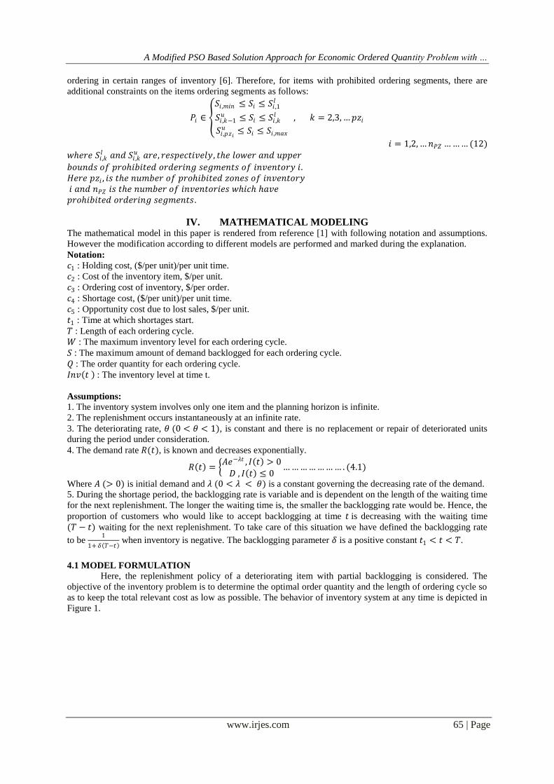
Figure 4: Inventory level 𝑰 𝒕 𝒗𝒔. 𝒕 𝒕𝒊𝒎𝒆 .

Replenishment is made at time 𝑡 = 0 and the inventory level is at its maximum 𝑊. Due to both the

market demand and deterioration of the item, the inventory level decreases during the period [0, 𝑡1] , and

ultimately falls to zero at 𝑡 = 𝑡1. Thereafter, shortages are allowed to occur during the time interval [𝑡1,𝑇] and

all of the demand during the period [𝑡1,𝑇] is partially backlogged.

As described above, the inventory level decreases owing to demand rate as well as deterioration during

inventory interval [0, 𝑡1]. Hence, the differential equation representing the inventory status is given by 𝑑𝐼𝑛𝑣 𝑡

𝑑𝑡+ 𝜃𝐼𝑛𝑣 𝑡 = −𝐴𝑒−𝜆𝑡 , 0 ≤ 𝑡 ≤ 𝑡1 ……… . (4.2)

with the boundary condition 𝐼𝑛𝑣 0 = 𝑊. The solution of equation (1) is

𝐼𝑛𝑣 𝑡 = 𝐴e−𝑡 λ−θ

λ − θ+ 𝑊 −

𝐴

λ − θ e−θ𝑡 ……… (4.3)

Since the inventory falls to zero at time 𝑡1, applying the condition to equation (2) gives

𝐼𝑛𝑣 𝑡1 = 𝐴e−𝑡1 λ−θ

λ − θ+ 𝑊 −

𝐴

λ − θ e−θ𝑡1 = 0…… (4.4)

From the above equation we can get the value of 𝑊 (maximum inventory level)

𝑊 = −𝐴 𝑒−𝑡1 𝜆−𝜃 − 1

𝜆 − 𝜃……… . . (4.5)

Where 𝑊 must satisfy 𝐿𝐵 ≤ 𝑊 ≤ 𝑈𝐵.

Now putting the value of equation (4.5) into equation (4.3)

𝐼𝑛𝑣 𝑡 = 𝐴𝑒−𝑡 𝜆−𝜃

𝜆 − 𝜃−𝐴 𝑒−𝑡1 𝜆−𝜃 − 1

𝜆 − 𝜃−

𝐴

𝜆 − 𝜃 𝑒−𝜃𝑡 . . (4.6)

By simplifying the equation (4), the inventory level at time 𝑡 can be given as

𝐼𝑛𝑣 𝑡 = −𝐴 −𝑒−𝑡 𝜆−𝜃 + 𝑒−𝑡1 𝜆−𝜃 𝑒−𝜃𝑡

𝜆 − 𝜃…… . . (4.7)

During the shortage interval [𝑡1,𝑇], the demand at time 𝑡 is partly backlogged at the fraction 1

1+𝛿 𝑇−𝑡 Thus, the

differential equation governing the amount of demand backlogged is as below. 𝑑𝐼𝑛𝑣 𝑡

𝑑𝑡=

𝐷

1 + 𝛿 𝑇 − 𝑡 , 𝑡1 < 𝑡 ≤ 𝑇…………… . (4.8)

with the boundary condition 𝐼 𝑡1 = 0 . The solution of equation (6) can be given by

𝐼𝑛𝑣 𝑡 =𝐷

𝛿{ln[1 + 𝛿(𝑇 − 𝑡)] − ln[1 + 𝛿(𝑇 − 𝑡1)]}, 𝑡1 ≤ 𝑡 ≤ 𝑇……… . (4.9)

Let 𝑡 = 𝑇 in (7), we obtain the maximum amount of demand backlogged per cycle as follows:

𝑆 = −𝐼𝑛𝑣 𝑇 =𝐷

𝛿ln 1 + 𝛿 𝑇 − 𝑡1 …………… (4.10)

Hence, the ordered quantity per cycle is given by



𝑄 = 𝑊 + 𝑆 =𝐴

𝜃 − 𝜆 𝑒 𝜃−𝜆 𝑡1 − 1 +

𝐷

𝜆ln 1 + 𝛿 𝑇 − 𝑡1 ………… . . (4.11)

Where 𝑄 must satisfy 𝑆𝑚𝑖𝑛 ≤ 𝑄 ≤ 𝑆𝑚𝑎𝑥 𝑎𝑛𝑑 𝑄 ∉ 𝑆Prohibited .

The inventory holding cost per cycle is

𝐻𝐶 = 𝑐1𝐼𝑛𝑣 𝑡 𝑑𝑡 =𝑐1𝐴

𝜃 𝜃 − 𝜆 𝑒−𝜆𝑡1 𝑒𝜃𝑡1 − 1 −

𝜃

𝜆 𝑒𝜆𝑡1 − 1 ……… . . (4.12)

𝑡1

0

The deterioration cost per cycle is

𝐷𝐶 = 𝑐2[𝑊 − 𝑅 𝑡 𝑑𝑡]𝑡1

0

= 𝑐2[𝑊 − 𝐴𝑒−𝜆𝑡 ]𝑡1

0

= 𝑐2𝐴 1

𝜃 − 𝜆 𝑒 𝜃−𝜆 𝑡1 − 1 −

1

𝜆 1 − 𝑒1

−𝜆𝑡 …… . . (4.13)

The shortage cost per cycle is

𝑆𝐶 = 𝑐4 − 𝐼 𝑡 𝑑𝑡 𝑇

𝑡1

= 𝑐4𝐷 𝑇 − 𝑡1

𝛿−

1

𝛿2ln 1 + 𝛿 𝑇 − 𝑡1 … . (4.14)

The opportunity cost due to lost sales per cycle is

𝐵𝐶 = 𝑐5 1 −1

1 + 𝛿 𝑇 − 𝑡 𝐷 𝑑𝑡 = 𝑐5𝐷 𝑇 − 𝑡1 −

1

𝛿ln 1 + 𝛿 𝑇 − 𝑡1 … (4.15)

𝑇

𝑡1

Therefore, the average total cost per unit time per cycle is

𝑇𝑉𝐶 ≡ 𝑇𝑉𝐶(𝑡1,𝑇)

= (holding cost + deterioration cost + ordering cost + shortage cost + opportunity cost due to lost sales)/ length

of ordering cycle

𝑇𝑉𝐶 = 1

𝑇

𝑐1𝐴

𝜃 𝜃 − 𝜆 𝑒−𝜆𝑡1 𝑒𝜃𝑡1 − 1 −

𝜃

𝜆 𝑒𝜆𝑡1 − 1 + 𝑐2𝐴

𝑒 𝜃−𝜆 𝑡1 − 1

𝜃 − 𝜆−

1 − 𝑒−𝜆𝑡1

𝜆

+ 𝑐3𝐷 𝑐4

𝜆+ 𝑐5 𝑇 − 𝑡1 −

ln 1 + 𝛿 𝑇 − 𝑡1

𝛿 … 4.16

Further simplification gives

𝑇𝑉𝐶 =1

𝑇 𝐴 𝑐1 + 𝜃𝑐2

𝜃 𝜃 − 𝜆 𝑒 𝜃−𝜆 𝑡1 − 𝜃 − 𝜆 𝑡1 − 1 −

𝐴 𝑐1 + 𝜃𝑐2

𝜃𝜆 1 − 𝜆𝑡1 − 𝑒−𝜆𝑡1 + 𝑐3

+𝐷 𝑐4 + 𝛿𝑐5

𝛿 𝑇 − 𝑡1 −

ln 1 + 𝛿 𝑇 − 𝑡1

𝛿 …… . .… (4.17)

Under the following constrains

𝑆𝑚𝑖𝑛 ≤𝐴

𝜃 − 𝜆 𝑒 𝜃−𝜆 𝑡1 − 1 +

𝐷

𝜆ln 1 + 𝛿 𝑇 − 𝑡1 ≤ 𝑆𝑚𝑎𝑥 … (4.18)

𝐴

𝜃 − 𝜆 𝑒 𝜃−𝜆 𝑡1 − 1 +

𝐷

𝜆ln 1 + 𝛿 𝑇 − 𝑡1 ∉ 𝑆Prohibited … (4.19)

𝐿𝐵 ≤ −𝐴 𝑒−𝑡1 𝜆−𝜃 − 1

𝜆 − 𝜃≤ 𝑈𝐵………… . (4.20)

The objective of the model is to determine the optimal values of 𝑡1 and 𝑇 in order to minimize the average total

cost per unit time (TVC) within the given constrains.

V. PARTICLE SWARM OPTIMIZATION (PSO) The PSO algorithm is inspired by the natural swarm behavior of birds and fish. It was introduced by

Eberhart and Kennedy in 1995 as an alternative to other ECTs, such as Ant Colony Optimization, Genetic

Algorithms (GA) or Differential Evolution (DE). Each particle in the population represents a possible solution

of the optimization problem, which is defined by its cost function. In each iteration, a new location (combination

of cost function parameters) of the particle is calculated based on its previous location and velocity vector

(velocity vector contains particle velocity for each dimension of the problem).The PSO algorithm works by

simultaneously maintaining several candidate solutions in the search space. During each iteration of the

algorithm, each candidate solution is evaluated by the objective function being optimized, determining the

fitness of that solution. Each candidate solution can be thought of as a particle “flying” through the fitness

landscape finding the maximum or minimum of the objective function. Initially, the PSO

algorithm chooses candidate solutions randomly within the search space. It should be noted that the PSO



algorithm has no knowledge of the underlying objective function, and thus has no way of knowing if any of the

candidate solutions are near to or far away from a local or global maximum. The PSO algorithm simply uses the

objective function to evaluate its candidate solutions, and operates upon the resultant fitness values.

Each particle maintains its position, composed of the candidate solution and its evaluated fitness, and

its velocity. Additionally, it remembers the best fitness value it has achieved thus far during the operation of the

algorithm, referred to as the individual best fitness, and the candidate solution that achieved this fitness, referred

to as the individual best position or individual best candidate solution. Finally, the PSO algorithm maintains the

best fitness value achieved among all particles in the swarm, called the global best fitness, and the candidate

solution that achieved this fitness, called the global best position or global best candidate solution.

The PSO algorithm consists of just three steps, which are repeated until some stopping condition is met:

1. Evaluate the fitness of each particle

2. Update individual and global best fitness‟s and positions

3. Update velocity and position of each particle

4. Repeat the whole process till the

The first two steps are fairly trivial. Fitness evaluation is conducted by supplying the candidate solution

to the objective function. Individual and global best fitness‟s and positions are updated by comparing the newly

evaluated finesses against the previous individual and global best fitness‟s, and replacing the best fitness‟s and

positions as necessary.

The velocity and position update step is responsible for the optimization ability of the PSO algorithm. The

velocity of each particle in the swarm is updated using the following equation:

𝑣 𝑖 + 1 = 𝑤 ∗ 𝑣 𝑖 + 𝑐1 ∗ 𝑝𝐵𝑒𝑠𝑡 − 𝑥 𝑖 + 𝑐2 ∗ 𝑔𝐵𝑒𝑠𝑡 − 𝑥 𝑖 ……… (5.1)

Modified PSO with chaos driven pseudorandom number perturbation

𝑣 𝑖 + 1 = 𝑤 ∗ 𝑣 𝑖 + 𝑐1 ∗ 𝑅𝑎𝑛𝑑 ∗ 𝑝𝐵𝑒𝑠𝑡 − 𝑥 𝑖 + 𝑐2 ∗ 𝑅𝑎𝑛𝑑 ∗ 𝑔𝐵𝑒𝑠𝑡 − 𝑥 𝑖 ……… (5.2)

A chaos driven pseudorandom number perturbation (𝑅𝑎𝑛𝑑) is used in the main PSO formula (Eq. (13)) that

determines new „„velocity‟‟ and thus the position of each particle in the next iterations (or migration cycle). The

perturbation facilities the better search in the available search space hence provides much better results.

𝑊𝑕𝑒𝑟𝑒: 𝑣(𝑖 + 1) − 𝑁𝑒𝑤 𝑣𝑒𝑙𝑜𝑐𝑖𝑡𝑦 𝑜𝑓 𝑎 𝑝𝑎𝑟𝑡𝑖𝑐𝑙𝑒. 𝑣(𝑖) − 𝐶𝑢𝑟𝑟𝑒𝑛𝑡 𝑣𝑒𝑙𝑜𝑐𝑖𝑡𝑦 𝑜𝑓 𝑎 𝑝𝑎𝑟𝑡𝑖𝑐𝑙𝑒. 𝑐1 , 𝑐2 − 𝑃𝑟𝑖𝑜𝑟𝑖𝑡𝑦 𝑓𝑎𝑐𝑡𝑜𝑟𝑠. 𝑝𝐵𝑒𝑠𝑡 − 𝐵𝑒𝑠𝑡 𝑠𝑜𝑙𝑢𝑡𝑖𝑜𝑛 𝑓𝑜𝑢𝑛𝑑 𝑏𝑦 𝑎 𝑝𝑎𝑟𝑡𝑖𝑐𝑙𝑒. 𝑔𝐵𝑒𝑠𝑡 − 𝐵𝑒𝑠𝑡 𝑠𝑜𝑙𝑢𝑡𝑖𝑜𝑛 𝑓𝑜𝑢𝑛𝑑 𝑖𝑛 𝑎 𝑝𝑜𝑝𝑢𝑙𝑎𝑡𝑖𝑜𝑛.

𝑅𝑎𝑛𝑑 − 𝑅𝑎𝑛𝑑𝑜𝑚 𝑛𝑢𝑚𝑏𝑒𝑟, 𝑖𝑛𝑡𝑒𝑟𝑣𝑎𝑙 0, 1 .𝐶𝑕𝑎𝑜𝑠 𝑛𝑢𝑚𝑏𝑒𝑟 𝑔𝑒𝑛𝑒𝑟𝑎𝑡𝑜𝑟 𝑖𝑠 𝑎𝑝𝑝𝑙𝑖𝑒𝑑 𝑜𝑛𝑙𝑦 𝑕𝑒𝑟𝑒.

𝑥(𝑖) − 𝐶𝑢𝑟𝑟𝑒𝑛𝑡 𝑝𝑜𝑠𝑖𝑡𝑖𝑜𝑛 𝑜𝑓 𝑎 𝑝𝑎𝑟𝑡𝑖𝑐𝑙𝑒. The new position of a particle is then given by (5.3), where 𝑥(𝑖 + 1) is the new position:

𝑥 𝑖 + 1 = 𝑥 𝑖 + 𝑣 𝑖 + 1 ………… . . (5.3)

Inertia weight modification PSO strategy has two control parameters 𝑤𝑠𝑡𝑎𝑟𝑡 and 𝑤𝑒𝑛𝑑 . A new w for each

iteration is given by (5.4), where 𝑖 stand for current iteration number and n for the total number of iterations.

𝑤 = 𝑤𝑠𝑡𝑎𝑟𝑡 − 𝑤𝑠𝑡𝑎𝑟𝑡 − 𝑤𝑒𝑛𝑑 ∗ 𝑖

𝑛…………… . (5.4)

Each of the three terms (𝑤 ∗ 𝑣 𝑖 , 𝑐1 ∗ 𝑅𝑎𝑛𝑑 ∗ 𝑝𝐵𝑒𝑠𝑡 − 𝑥 𝑖 𝑎𝑛𝑑 𝑐2 ∗ 𝑅𝑎𝑛𝑑 ∗ 𝑔𝐵𝑒𝑠𝑡 − 𝑥 𝑖 of the velocity

update equation have different roles in the PSO algorithm.

The first term 𝑤 is the inertia component, responsible for keeping the particle moving in the same

direction it was originally heading. The value of the inertial coefficient 𝑤 is typically between 0.8 and 1.2,

which can either dampen the particle‟s inertia or accelerate the particle in its original direction. Generally, lower

values of the inertial coefficient speed up the convergence of the swarm to optima, and higher values of the

inertial coefficient encourage exploration of the entire search space.

The second term 𝑐1 ∗ 𝑅𝑎𝑛𝑑 ∗ 𝑝𝐵𝑒𝑠𝑡 − 𝑥 𝑖 called the cognitive component, acts as the particle‟s

memory, causing it to tend to return to the regions of the search space in which it has experienced high

individual fitness.

The cognitive coefficient 𝑐1 is usually close to 2, and affects the size of the step the particle takes toward its

individual best candidate solution 𝑝𝐵𝑒𝑠𝑡.



The third term 𝑐2 ∗ 𝑅𝑎𝑛𝑑 ∗ 𝑔𝐵𝑒𝑠𝑡 − 𝑥 𝑖 , called the social component, causes the particle to move to the best

region the swarm has found so far. The social coefficient 𝑐2 is typically close to 2, and represents the size of the

step thfe particle takes toward the global best candidate solution 𝑔𝐵𝑒𝑠𝑡 the swarm has found up until that point.

VI. CHAOTIC MAPS This section contains the description of discrete chaotic maps used as the chaotic pseudorandom

inventory for PSO. In this research, direct output iterations of the chaotic map were used for the generation of

real numbers for the main PSO formula that determines new velocity, thus the position of each particle in the

next iteration (See (2) in section 2). The procedure of embedding chaotic dynamics into evolutionary algorithms

is given in [15][16] while the techniques for selecting proper parameter values in discussed in [17].

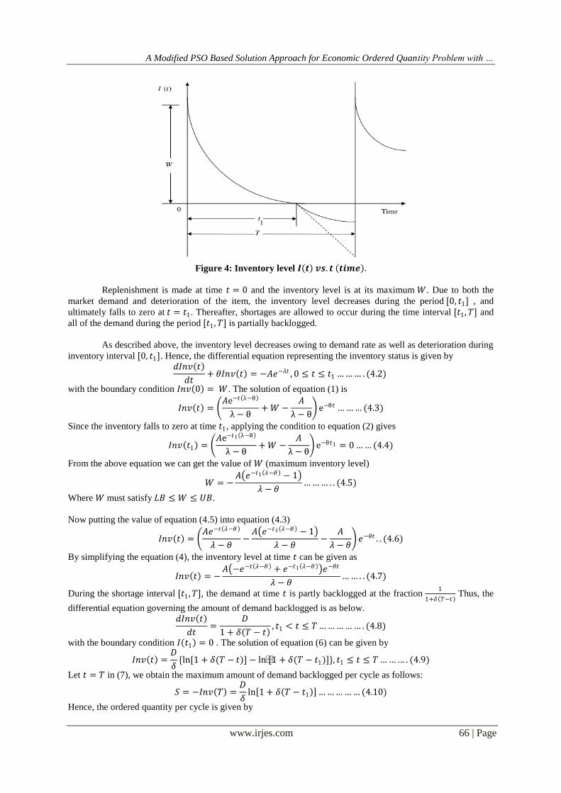
6.1 LOGISTIC MAP

The logistic map is a polynomial mapping (equivalently, recurrence relation) of degree 2, shows the

complex, chaotic behavior from very simple non-linear dynamical equations. Mathematically, the logistic map

is written

𝑋𝑛+1 = 𝜇𝑋𝑛 1 − 𝑋𝑛 …………… (6.1)

Figure 6:1: Plot of logistic map 𝝁 = 𝟒 and 𝑿𝟎 = 𝟎.𝟔𝟑 after 100 iterations.

6.2. LOZI MAP

The Lozi map is a simple discrete two-dimensional chaotic map. The map equations are given in (17).

𝑋𝑛+1 = 1 − 𝑥 𝑋𝑛 + 𝑏𝑌𝑛 ………… . (6.2𝑎)

𝑌𝑛+1 = 𝑋𝑛 ……………… . (6.2𝑏)

Figure 6:2: The 2D Plot of Lozi Map for 𝒂 = 𝟏.𝟕,𝒃 = 𝟎.𝟓 after 1000 iterations



Figure 6:3: Plot of Lozi map for 𝒂 = 𝟏.𝟕,𝒃 = 𝟎.𝟓 after 100 iterations

VII. IMPLEMENTATION OF IMPROVED PSO ALGORITHM FOR ECONOMIC

ORDERED QUANTITY (EOQ) PROBLEMS Since the decision variables in EOQ problems are 𝑡1 and 𝑇 with 𝑆 = {𝑆1 , 𝑆2 ,… . , 𝑆𝑛 } where 𝑆𝑖 ordering

quantity of 𝑖𝑡𝑕 inventory, the structure of a particle is composed of a set of elements corresponding to

the [𝑡1,𝑇, 𝑆]. Therefore, particle‟s position at iteration 𝑘 can be represented as the vector

𝑋𝑖𝑘 = 𝑃𝑖1

𝑘 ,𝑃𝑖2𝑘 …… . . ,𝑃𝑖𝑚

𝑘 where 𝑚 = 𝑛 + 2 and 𝑛 is the number of inventories. The velocity of particle 𝑖 corresponds to the generation updates for all inventories. The process of the proposed PSO algorithm can be

summarized as in the following steps.

1. Initialize the position and velocity of a population at random while satisfying the constraints.

2. Update the velocity of particles.

3. Modify the position of particles to satisfy the constraints, if necessary.

4. Generate the trial vector through operations presented in section 4.

5. Update and Go to Step 2 until the stopping criteria is satisfied.

Figure 7: Flow Chart of the Proposed Algorithm.



VIII. SIMULATION RESULTS The proposed IPSO approach is applied to three different inventory systems explained in section 3 and

evaluated by all three PSO models as follows:

• The conventional PSO

• The PSO with chaotic sequences

• The PSO with alternative chaotic operation

The simulation of all algorithms is performed using MATLAB. The population size 𝑁𝑃 and maximum

iteration number 𝑖𝑡𝑒𝑟𝑚𝑎𝑥 are set as 100 and 100, respectively. 𝑤𝑚𝑎𝑥 and 𝑤𝑚𝑖𝑛 are set to 0.9 and 0.1

respectively because these values are widely accepted and verified in solving various optimization problems.

The list of all values used for the system are shown in the table below

Table 1: parameter values used for different PSO algorithms

Name of Variable Value Assigned

𝑐1 2

𝑐2 1

𝑤𝑚𝑎𝑥 0.9

𝑤𝑚𝑖𝑛 0.1

𝜇 (logistic map) 4.0

𝑘 (logistic map) 0.63

𝑎 (lozi map) 1.7

𝑏 (lozi map) 0.5

Total Particles 100

Maximum Iterations 100

Table 2: values of system variables:

Variable Value

Variable Name Scenario 1 Scenario 2

𝐴 12 12

𝜃 0.08 0.08

𝛿 2 2

𝜆 0.03 0.03

𝑐1 0.5 0.5

𝑐2 1.5 1.5

𝑐3 10 10

𝑐4 2.5 2.5

𝑐5 2 2

𝐷 8 8

𝛼 5 5

𝛽 10 10

𝛾 0.04 N/A

𝑆𝑚𝑖𝑛 1 1

𝑆𝑚𝑎𝑥 100 95

𝑁 N/A 15

𝑆𝑠𝑒𝑔 N/A 6

𝛽1 N/A 10



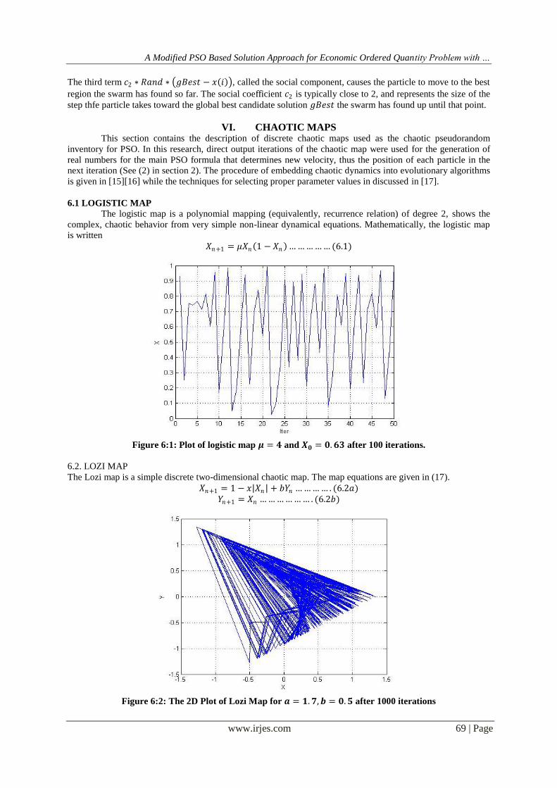
Figure 8.1: surface plot for the normal inventory system. With respect to 𝑡1 (the time at which shortage starts)

and 𝑇(ordering cycle time) the figure shows a smooth and continuous curve and hence can be solved by

analytical technique also.

Figure 8.2: surface plot for the order segment dependent inventory cost type model. With respect to 𝑡1 (the time

at which shortage starts) and 𝑇(ordering cycle time) the figure shows much abrupt variations and many

discontinuities in the curve and hence can be very difficult to solve by analytical techniques.

Figure 8.3: the value of objective function (fitness value or TVC) at every iteration of PSO for model 1.



Figure 8.4: the best values of variables 𝑡1 and 𝑇 for all three PSO for model 1.

Table 3: Best Fitness Values by all three PSO for model 1.

Type of PSO Best Fitness (TVC)

PSO 11.6625

PSO1 11.4125

PSO2 11.2736

IX. CONCLUSION AND FUTURE SCOPE In this paper presents the mathematical model for inventories systems Considering Order Size Limits,

Stock Limits and Prohibited Ordering Segments the paper also presents the derivations for evaluation of the

function parameters for practical applications and finally it proposes an efficient approach for solving EOQ

problem under the mentioned constrains applied simultaneously. Which may not be solved by analytical

approach hence the meta-heuristic approach has been accepted in the form of standard PSO furthermore the

performance of standard PSO is also enhanced by alternative use of two different chaotic maps for velocity

updating finally it is applied to the EOQ problem for the inventory models discussed above and tested for

different systems and objectives. The simulation result shows the proposed approach finds the solution very

quickly with much lesser mathematical complexity. The simulation also verifies the superiority of proposed

PSO over the standard PSO algorithm and supports the idea that switching between different chaotic

pseudorandom number generators for updating the velocity of particles in the PSO algorithm improves its

performance and the optimization process. The results for different experiments are collected with different

settings and results compared with other methods which shows that the proposed algorithm improves the results

by considerable margin.

REFERENCE [1]. Liang-Yuh OUYANG, Kun-Shan WU, Mei-Chuan CHENG, “AN INVENTORY MODEL FOR

DETERIORATING ITEMS WITH EXPONENTIAL DECLINING DEMAND AND PARTIAL

BACKLOGGING”, Yugoslav Journal of Operations Research 15 (2005), Number 2, 277-288.

[2]. Kai-Wayne Chuang, Chien-Nan Lin, and Chun-Hsiung Lan “Order Policy Analysis for Deteriorating

Inventory Model with Trapezoidal Type Demand Rate”, JOURNAL OF NETWORKS, VOL. 8, NO. 8,

AUGUST 2013.

[3]. G.P. SAMANTA, Ajanta ROY “A PRODUCTION INVENTORY MODEL WITH

DETERIORATING ITEMS AND SHORTAGES”, Yugoslav Journal of Operations Research 14

(2004), Number 2, 219-230.

[4]. Jonas C.P. Yu “A collaborative strategy for deteriorating inventory system with imperfect items and

supplier credits”, Int. J. Production Economics 143 (2013) 403–409.

[5]. S. Kar, T. K. Roy, M. Maiti “Multi-objective Inventory Model of Deteriorating Items with Space

Constraint in a Fuzzy Environment”, Tamsui Oxford Journal of Mathematical Sciences 24(1) (2008)

37-60 Aletheia University.



[6]. Vinod Kumar Mishra , Lal Sahab Singh “Deteriorating Inventory Model with Time Dependent

Demand and Partial Backlogging”, Applied Mathematical Sciences, Vol. 4, 2010, no. 72, 3611 – 3619.

[7]. Lianxia Zhao “An Inventory Model under Trapezoidal Type Demand, Weibull-Distributed

Deterioration, and Partial Backlogging”, Hindawi Publishing Corporation Journal of Applied

Mathematics Volume 2014, Article ID 747419, 10 pages.

[8]. Xiaohui Hu, Russell Eberhart “Solving Constrained Nonlinear Optimization Problems with Particle

Swarm Optimization”,

[9]. Tetsuyuki Takahama, Setsuko Sakai “Constrained Optimization by Combining the α Constrained

Method with Particle Swarm Optimization”, Soft Computing as Transdisciplinary Science and

Technology Advances in Soft Computing Volume 29, 2005, pp 1019-1029.

[10]. Kuo-Lung Hou, Yung-Fu Huang and Li-Chiao Lin” An inventory model for deteriorating items with

stock-dependent selling rate and partial backlogging under inflation” African Journal of Business

Management Vol.5 (10), pp. 3834-3843, 18 May 2011.

[11]. Nita H. Shah and Munshi Mohmmadraiyan M. “AN ORDER-LEVEL LOT-SIZE MODEL FOR

DETERIORATING ITEMS FOR TWO STORAGE FACILITIES WHEN DEMAND IS

EXPONENTIALLY DECLINING”, REVISTA INVESTIGACIÓN OPERACIONAL VOL., 31 , No.

3, 193-199 , 2010.

[12]. Hui-Ling Yang “A Partial Backlogging Inventory Model for Deteriorating Items with Fluctuating

Selling Price and Purchasing Cost”, Hindawi Publishing Corporation Advances in Operations Research

Volume 2012, Article ID 385371, 15 pages.

[13]. Ibraheem Abdul and Atsuo Murata “An inventory model for deteriorating items with varying demand

pattern and unknown time horizon”, International Journal of Industrial Engineering Computations 2

(2011) 61–86.

[14]. Ching-Fang Lee, Chien-Ping Chung “An Inventory Model for Deteriorating Items in a Supply Chain

with System Dynamics Analysis”, Procedia - Social and Behavioral Sciences 40 ( 2012 ) 41 – 51.

[15]. Michal Pluhacek, Roman Senkerik, Ivan Zelinka and Donald Davendra “PERFORMANCE

COMPARISON OF EVOLUTIONARY TECHNIQUES ENHANCED BY LOZI CHAOTIC MAP IN

THE TASK OF REACTOR GEOMETRY OPTIMIZATION”, Proceedings 28th European Conference

on Modelling and Simulation ©ECMS.

[16]. O.T. Altinoz A.E. Yilmaz G.W. Weber “Application of Chaos Embedded Particle Swarm Optimization

for PID Parameter Tuning”, Int. J. of Computers, Communication and Control (Date of submission:

November 24, 2008).

[17]. Magnus Erik, Hvass Pedersen “Good Parameters for Particle Swarm Optimization”, Technical Report

no. HL1001 2010.