Improving Spatiotemporal Stability for Object Detection and Classification

Improving Spatiotemporal Stability for Object Detection

and Classification

Albert Y. C. Chen, Ph.D. Computer Scientist @ Tandent Vision

2015/03/27

Videos, lots of them.

0

20

40

60

80

2007 2008 2009 2010 2011 2012

Hours of videos uploaded to Youtube every minute

Goal: automatically analyze, organize, and archive videos.

Typical Approaches:Classifiers, classifiers, classifiers

•Video nouns, e.g., sky, tree, building, car, etc.•Video noun structures, e.g., horizontal flat surfaces, vertical surfaces, non-support surfaces, etc.•Video verbs, e.g., diving, bench press, punch.

Results are far from perfect

for example, in

Joint Segmentation and Classification (multiple semantic class pixel labeling)

Example annotations Object segmentation Class segmentation

Difficult objects masked

Image

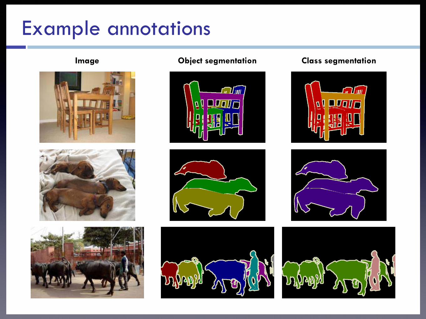
Example annotations Object segmentation Class segmentation Image

State-of-the-art results from Pascal VOC 2012

Segmentation Challenge

Example segmentations Image Ground truth

NUS_DET_SPR_GC_SP BONN_O2PCPMC_FGT_SEGM





Example Segmentations Image Ground truth


Apply these object classifiers to videos, frame by frame?

Inputframe

Ground truth labels

2D MRF results

00001TP_008820 00001TP_008850

VGSresults

00001TP_008880Name

Markov Random Field (MRF) for modeling Spatiotemporal Priors

spati

al

hidde

n lab

els

obse

rved

noisy

labe

lstemporal

first order spatial neighborhood

higher order spatial neighborhood

temporalneighborhood

Generic MRF Formulation for classification taks

E2 (mµ,m⌫) = 1� � (mµ,m⌫)

E [{mµ : µ 2 G}]

=X

µ2G

E1 (I (S [µ]) ,mµ) + �X

hµ,⌫i

E2 (mµ,m⌫)

E1 (I (S [µ]) ,mµ) = � logP⇣mµ

�� I (S [µ])⌘

Major technical contributions, MRF for modeling Spatiotemporal Priors

Name Application Description

Bilayer MRFVideo Label Propagation

An additional layer of hidden variables to model the motion v.s. appearance model weights.

Higher Order Proxy

Neighborhood

Joint segmentation and classification

Longer range spatial smoothness with traditional 1st

order neighborhood.

Video Graph-Shifts

Joint segmentation and classification

in videos

Simultaneously estimate the motion priors while doing

multiple semantic class labeling.

Subproblem 1 Bootstrapping the Classifier

Training process by using Hierarchical Supervoxels

The inconsistent and time consuming task of pixel labeling

Seq05VD_f02400Seq05VD_f02370Seq05VD_f02340

input

frame

semantic

object

label

roadsidewalk

sign

From the Cambridge Video Driving Dataset

Video pixel label propagation

FG

Traditional Spatial Propagation

Pixel label map

Label a subset of pixels

BG

Spatio-temporal Propagation

time

Optical Flow should do it?

Bidirectional optical flow frame 20

Black & Anadan Classic+NL

Bidirectional optical flow frame 60

Black & Anadan Classic+NL

Maybe a different optical flow algorithm?

Why optical flow alone fails

a hole occurs the dragging effect

Forward Flow Reverse Flow

multiple incomingflows

t t+1 t t+1

Train a appearance model on the user annotated frame?

0

10

20

30

40

50

60

70

80

90

100

1 11 21 31 41 51 61 71

!"#$%&#'(#$)*#&+,-'!../$%.0'1"

#$'23#'4#5/#-.#'

X:do-nothing

M:forward-flow

A:patch

Try again?

Motion-only Propagation Appearance-only Propagation50.00

55.00

60.00

65.00

70.00

75.00

80.00

85.00

90.00

95.00 100.00

1 11 21 31 41 51 61 71 81

!"#$%&#'(#$)*#&+,-'!../$%.0'1"

#$'23#'4#5/#-.#'

X:do-nothing

M:forward-flow

A:patch

Maybe we should do something like this?

app.app.

flow

flow

both

both

both

both

flow

app.

Turns out to be an optical flow reliability estimation problem

How good is our Motion vs Appearance (MvA) weights?

40

80

o. flow only

The Container Sequence

input image GT label app. onlyour method

40

80

input image GT label our method o. flow only app. only

The Garden Sequence

Well, there’s still problems-1

0.4

0.5

0.6

0.7

0.8

0.9

1

1 11 21 31 41 51 61 71

How to Weigh between Mot and App?

Fixed weight for all pixel

Naïve cross-correlation

Occlusion-aware cross corr.

Bidirectional flow consistency

Well, there’s still problems-2

Initial Noisy WvA weight map

Optimized WvA map with our bilyaer MRF

bus

socc

er

Target framefor propagation Ground Truth Label

Our bilayer MRF for Label Propagation

Observednoisy values

(Hidden true pixel labels)

(Hidden true WvA weights)

1st layer of MRF

2nd layer of MRF

label change at causes to change

as well as causing the WvA layer's energy to change

Our proposed Bilayer MRF for Video Pixel Label Pixel Label Propagatoin

Resultsframe 1 frame 75frame 50frame 25

stef

an

0

0.1

0.2

0.3

0.4

0.5

0.6

0.7

1 11 21 31 41 51 61 71

Stefan (tenis) Sequence

Appearance uni-model

Appearance multi-model

Do nothing

Bidirectional flow

Bad (fixed) WvA weights

Our method

Resultsso

ccer

frame 1 frame 75frame 50frame 25

0

0.1

0.2

0.3

0.4

0.5

0.6

0.7

0.8

0.9

1

1 11 21 31 41 51 61

Soccer Sequence


Appearance multi-model

Do nothing

Bidirectional flow

Our method

Bad WvA weights

Resultsbu

s

frame 1 frame 75frame 50frame 25

0

0.1

0.2

0.3

0.4

0.5

0.6

0.7

0.8

0.9

1

1 11 21 31 41 51 61 71

Bus Sequence

Do nothing

Bidirectional flow


Bad (fixed) MvA weight

Our method

Good, but far from perfect

• Overall accuracy still low

• Object Boundaries crossed

• Optical flow reliability estimation still noisy

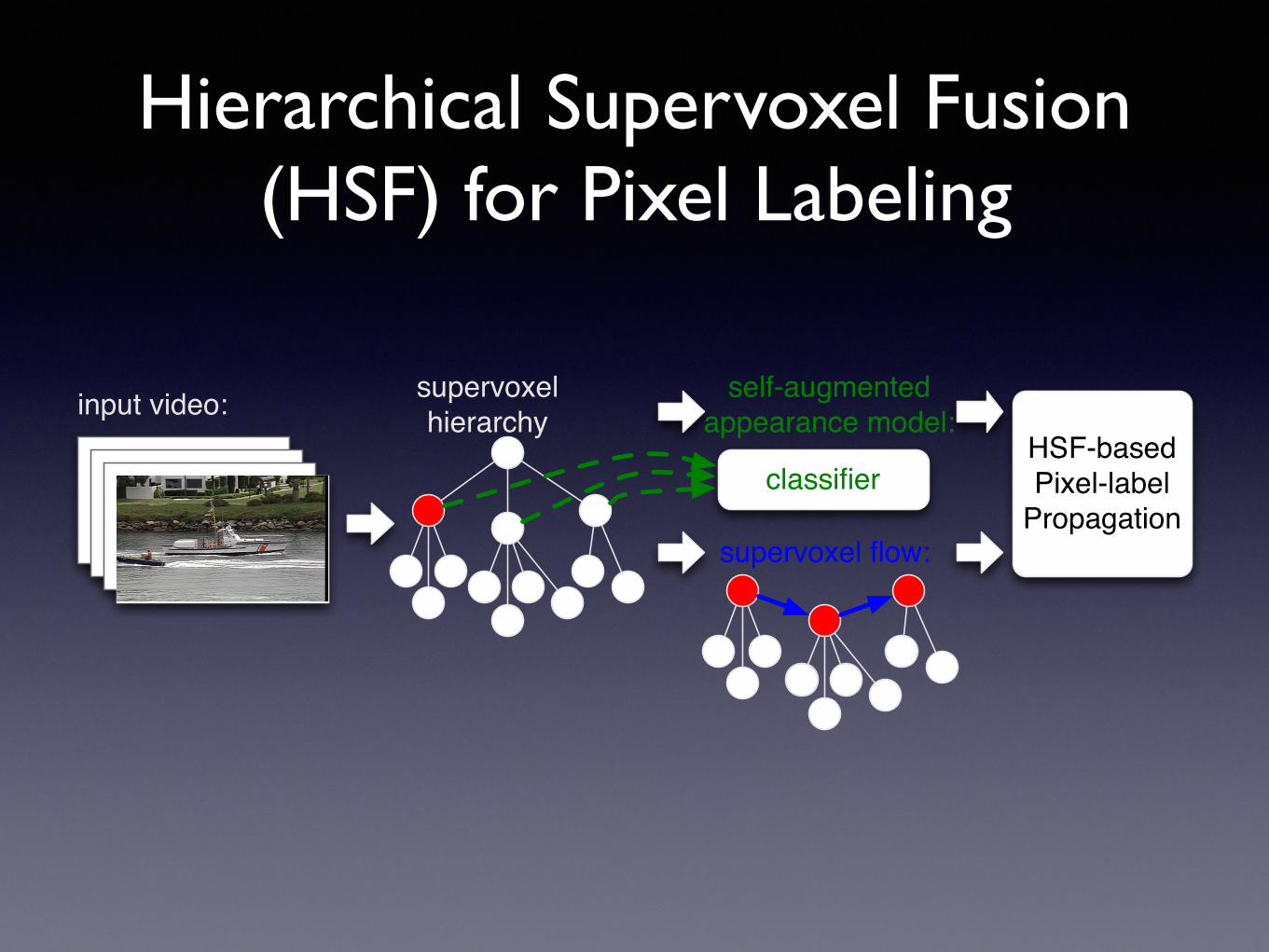
Hierarchical Supervoxel Fusion (HSF) for Pixel Labeling

input video: supervoxelhierarchy

self-augmented appearance model:

supervoxel flow:

classifierHSF-basedPixel-label

Propagation

What does HSF buy us?

• 100x more data for the appearance model.

• Supervoxel-level correspondences instead of just pixel-level optical flow.

• State-of-the-art pixel label propagation performance.

Supervoxel Hierarchy and the “right scale”

The HSF Process

y

Hierarchical Supervoxel Fusion

x

t

Label Consistency Maps

SupervoxelHierarchy

y

x

t

vehicle flower tree

y

x

t

input video:

Automatic Selection of the Maximum Hierarchy Height

Bus tree horse car flower sign road24x 3x 48x 33x 8x 18x

Container bldg grass tree sky water road boat91x 109x 93x 100x 90x 116x 89x

Garden bldg tree sky flower96x 54x 31x 60x

Ice face sign road body37x 22x 89x 65x

Paris tree face book body113x 127x 105x 44x

Salesman tree face book111x 102x 84x

Soccer grass tree face sign dog body66x 83x 14x 28x 15x 62x

Stefan grass face sign chair body83x 1x 75x 1x 83x

Camvid bldg tree/grasssky road pavemt. concr. roadmk.6x 25x 1170x 176x 76x 20x 1756x

Table 3.1: Increase in training set size of the self-augmented training set (donethrough Hierarchical Supervoxel Fusion) over the original training set.

Seq\ Lv 6 7 8 9 10 11 12 13 14 15Bus 4.22% 6.11% 8.93% 9.44% 10.71% 18.57% 22.00% 27.55% 35.96% 47.36%Container 0.08% 0.07% 0.16% 0.44% 0.86% 2.37% 3.28% 6.69% 14.11% 21.75%Garden 0.83% 1.74% 2.66% 3.90% 6.21% 11.37% 20.12% 29.74% 30.43% 50.68%Ice 0.11% 0.28% 0.89% 1.54% 1.99% 2.21% 2.32% 2.32% 2.41% 27.04%Paris 0.38% 0.46% 0.73% 1.30% 2.02% 3.68% 9.02% 9.48% 11.32% 13.93%Salesman 0.31% 0.46% 0.66% 1.58% 4.00% 7.18% 10.23% 20.99% 24.17% 25.01%Soccer 0.29% 0.49% 0.61% 1.31% 1.57% 1.70% 5.43% 19.12% 33.89% 38.57%Stefan 0.42% 0.74% 1.10% 1.38% 1.69% 1.91% 2.45% 3.97% 6.73% 39.70%Camvid 1.72% 3.55% 6.23% 7.51% 11.06% 18.45% 25.84%

Table 3.2: Automatic Hierarchy Height Selection by computing the SupervoxelBoundary Error on the user annotated frame. The shaded levels are discarded sincetoo many of the supervoxels violate the user-defined boundaries.

algorithm needs to estimate is logarithmic to the number of pixels. On the same machine us-

ing Matlab implementations, our supervoxel flow algorithm takes only seconds per frame,

while per-pixel optical flow based propagation takes minutes to hours (based on the code

released with [35]. By exploiting the supervoxel hierarchy structure and merging the su-

pervoxel flows computed at different levels (similar to computing optical flows at different

46

Supervoxel boundary error on the user annotated frame.

The Self-augmented Appearance Model

Bus tree horse car flower sign road24x 3x 48x 33x 8x 18x

Container bldg grass tree sky water road boat91x 109x 93x 100x 90x 116x 89x

Garden bldg tree sky flower96x 54x 31x 60x

Ice face sign road body37x 22x 89x 65x

Paris tree face book body113x 127x 105x 44x

Salesman tree face book111x 102x 84x

Soccer grass tree face sign dog body66x 83x 14x 28x 15x 62x

Stefan grass face sign chair body83x 1x 75x 1x 83x

Camvid bldg tree/grasssky road pavemt. concr. roadmk.6x 25x 1170x 176x 76x 20x 1756x

Table 3.1: Increase in training set size of the self-augmented training set (donethrough Hierarchical Supervoxel Fusion) over the original training set.

Seq\ Lv 6 7 8 9 10 11 12 13 14 15Bus 4.22% 6.11% 8.93% 9.44% 10.71% 18.57% 22.00% 27.55% 35.96% 47.36%Container 0.08% 0.07% 0.16% 0.44% 0.86% 2.37% 3.28% 6.69% 14.11% 21.75%Garden 0.83% 1.74% 2.66% 3.90% 6.21% 11.37% 20.12% 29.74% 30.43% 50.68%Ice 0.11% 0.28% 0.89% 1.54% 1.99% 2.21% 2.32% 2.32% 2.41% 27.04%Paris 0.38% 0.46% 0.73% 1.30% 2.02% 3.68% 9.02% 9.48% 11.32% 13.93%Salesman 0.31% 0.46% 0.66% 1.58% 4.00% 7.18% 10.23% 20.99% 24.17% 25.01%Soccer 0.29% 0.49% 0.61% 1.31% 1.57% 1.70% 5.43% 19.12% 33.89% 38.57%Stefan 0.42% 0.74% 1.10% 1.38% 1.69% 1.91% 2.45% 3.97% 6.73% 39.70%Camvid 1.72% 3.55% 6.23% 7.51% 11.06% 18.45% 25.84%

Table 3.2: Automatic Hierarchy Height Selection by computing the SupervoxelBoundary Error on the user annotated frame. The shaded levels are discarded sincetoo many of the supervoxels violate the user-defined boundaries.

algorithm needs to estimate is logarithmic to the number of pixels. On the same machine us-

ing Matlab implementations, our supervoxel flow algorithm takes only seconds per frame,

while per-pixel optical flow based propagation takes minutes to hours (based on the code

released with [35]. By exploiting the supervoxel hierarchy structure and merging the su-

pervoxel flows computed at different levels (similar to computing optical flows at different

46

Increase in the number of pixels available for training the appearance model.

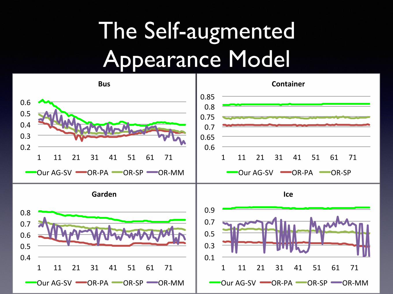
0.2$0.3$0.4$0.5$0.6$

1$ 11$ 21$ 31$ 41$ 51$ 61$ 71$

Bus$

Our$AG0SV$ OR0PA$ OR0SP$ OR0MM$

0.6$0.65$0.7$

0.75$0.8$

0.85$

1$ 11$ 21$ 31$ 41$ 51$ 61$ 71$

Container)

Our$AG1SV$ OR1PA$ OR1SP$

0.4$0.5$0.6$0.7$0.8$

1$ 11$ 21$ 31$ 41$ 51$ 61$ 71$

Garden'


0.1$0.3$0.5$0.7$0.9$

1$ 11$ 21$ 31$ 41$ 51$ 61$ 71$

Ice$


The Self-augmented Appearance Model

Supervoxel flow propagation performance-1

0.2$

0.4$

0.6$

0.8$

1$ 11$ 21$ 31$ 41$ 51$ 61$ 71$ 81$

Bus$

HD.OF$ SF.BI.OF$ SVXL.flow$

0.2$0.4$0.6$0.8$1$

1$ 11$ 21$ 31$ 41$ 51$ 61$ 71$ 81$

Garden'


0.4$0.5$0.6$0.7$0.8$0.9$1$

1$ 11$ 21$ 31$ 41$ 51$ 61$ 71$

Ice$

HD/OF$ SF/BI/OF$ SVXL/flow$

0.5$0.6$0.7$0.8$0.9$1$

1$ 11$ 21$ 31$ 41$ 51$ 61$ 71$ 81$

Container)


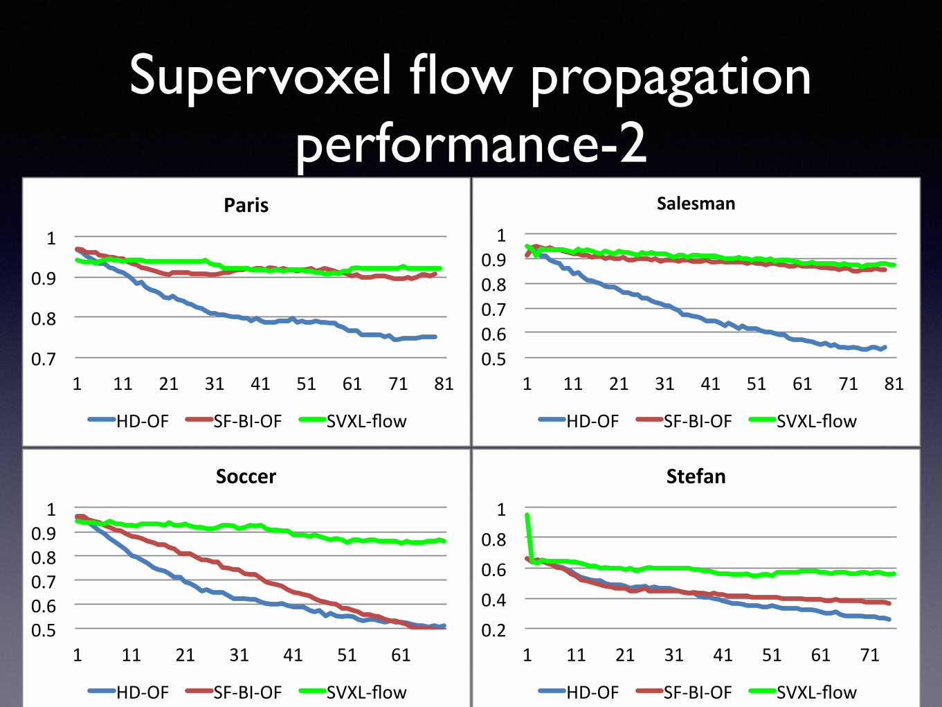
Supervoxel flow propagation performance-2

0.7$

0.8$

0.9$

1$

1$ 11$ 21$ 31$ 41$ 51$ 61$ 71$ 81$

Paris&


0.5$0.6$0.7$0.8$0.9$1$

1$ 11$ 21$ 31$ 41$ 51$ 61$

Soccer&


0.5$0.6$0.7$0.8$0.9$1$

1$ 11$ 21$ 31$ 41$ 51$ 61$ 71$ 81$

Salesman(


0.2$0.4$0.6$0.8$1$

1$ 11$ 21$ 31$ 41$ 51$ 61$ 71$

Stefan'


Finally, putting everything together, our Hierarchical

Supervoxel Fusion-based Pixel Label Propagation

Subproblem 2 Random Field Priors for

Improving the Spatiotemporal Robustness of Classifiers

Problems with Traditional First Order Neighborhood

µ

ν

ν

ν

ν

µ µ

µ µ

Higher-order Proxy Neighbors

µ

ν

ν

ν

ν

E [{mµn : µn 2 Gn}] = �1

X

µn2Gn

E1 (µn,mµn)

+�2X

µn2Gn

( (µn,mµn)

X

hµn,⌫ni

E2 (µ

n, ⌫n,mµn ,m⌫n)

+�02X

⌫n2Gn

(⌫n,mµn)X

h⌫n,⌧ni\hµn,⌫ni

E2 (⌫n, ⌧n,mµn ,m⌧n)

�)

Energy Minimization via the Graph-Shifts Algorithm

Shift

µ µν ν

P(ν) P(ν) P(µ)P(µ)

Recursive Computation of the Energy

E1 (µn,mµn

) =

⇢E1 (I (S [µn

]) ,mµn) if n = 0P

µn�12C(µn) E1

�µn�1,mµn�1

�otherwise

E2 (µn, ⌫n,mµn ,m⌫n

) =

8><

>:

E2 (mµn ,m⌫n) if n = 0P

µn�12C(µn)⌫n�12C(⌫n)hµn�1,⌫n�1i

E2

�µn�1, ⌫n�1,mµn�1 ,m⌫n�1

�otherwise

The overall energy, specified for level 0, is computed at any level by: E [{mµn : µn 2 Gn}] = �1

X

µn2Gn

E1 (µn,mµn)

+�2X

µn2Gn

(µn,mµn)

X

hµn,⌫ni

E2 (µn, ⌫n,mµn ,m⌫n)

�

where (µn,mµn) =

��D0(µn)��

Pa2D0(µn)

Pha,bi �

⇣An(a), An(b)

⌘

The Shift-Gradient is defined as�E (mµn ! m̂µn)

= E [{m̂µn : µn 2 Gn}]� E [{mµn : µn 2 Gn}]= �1 [E1 (µ

n, m̂µn)� E1 (µn,mµn)]

+ �2

(X

µn2Gn

(µn, m̂µn)

X

hµn,⌫ni

E2 (µn, ⌫n, m̂µn ,m⌫n)

�

�X

µn2Gn

(µn,mµn)

X

hµn,⌫ni

E2 (µn, ⌫n,mµn ,m⌫n)

�).

Visualizing the Graph-Shifts Process and Hierarchy

Input Image lv. 1 lv. 2 lv. 3 lv. 4 lv. 5 lv. 6

The Hierarchy

Input Label shift #0 shift #20 shift #60shift #40

The Energy Minimization Process

Efficiency Improvements of using HOPS

Input Ground Truth Classifier only First-order HOPS

Probability maps output by the classifier, and share by first-order and HOPS's E1 term:void sky water road grass tree(s)

mountain animal/man building bridge

4830 shifts 3769 shifts-22%

vehicle coastline

Efficiency Improvements of using HOPS

Input Ground Truth Classifier only First-order HOPS

Probability maps output by the classifier, and share by first-order and HOPS's E1 term:void sky water road grass tree(s)

2042 shifts 1868 shifts-8.6%

mountain animal/man building bridge vehicle coastline

Qualitative Results of HOPS on the MSRC-21 dataset

Legend void building grass tree cow horse sheep sky mountain aeroplane water facecar bicycle flower sign bird book chair road cat dog body boat

Image

Labels

Firstorder

HOPS

Examples of HOPS outperforming first order neighborhood models Mislabeling by HOPS

Classifier only

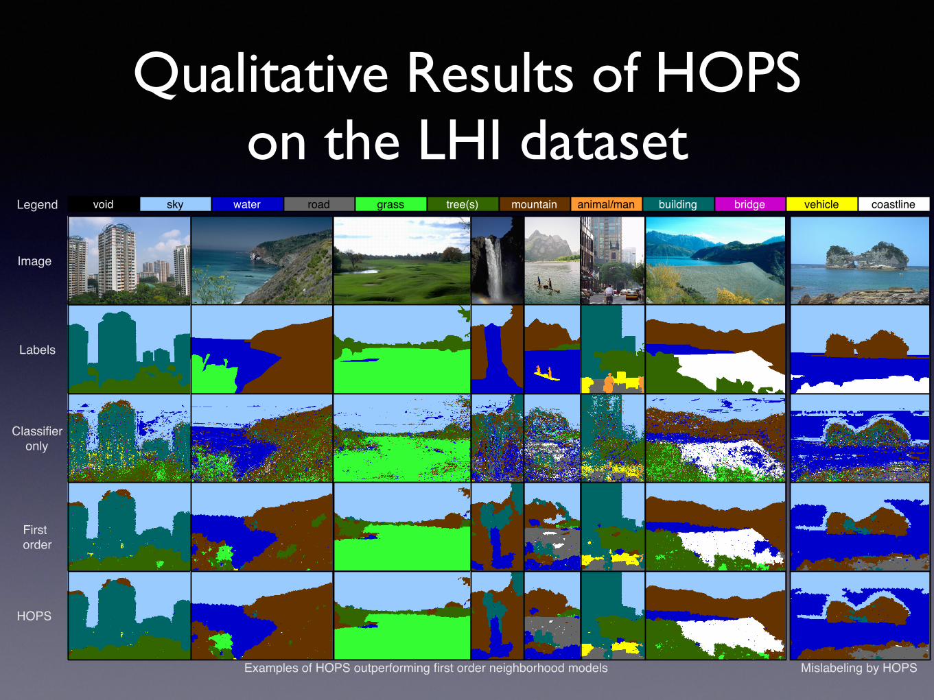
Qualitative Results of HOPS on the LHI dataset

Examples of HOPS outperforming first order neighborhood models Mislabeling by HOPS

void sky water road grass tree(s) mountain animal/man building bridge vehicle coastlineLegend

Image

Labels

Firstorder

HOPS

Classifier only

Quantitative Results on the MSRC-21 and LHI datasetsTable 4.1: Comparison of overall accuracy rate on the LHI dataset

Classifier-Only First Order HOPSOverall Accuracy 59.71 72.42 73.48Improvement over classifier-onlyoverall accuracy

12.71 13.77

Percentage gained over first-orderneighborhood’s improvement

8.34%

Table 4.2: Comparison of overall accuracy rate on the MSRC dataset


18.86 19.17%


1.64%

The optimum weights for the energy models are estimated (learned) during the train-

ing phase, where l1 = 0.7, l2 = 0.3 for first order neighborhood, and l1 = 0.6, l2 = 0.1,

and l

02 = 0.3 for HOPS on both datasets. Note that all images’ long side (either width or

height, depending on either its in landscape or portrait format) in the LHI dataset are 360

pixels, while the MSRC dataset images have a long side of only 200 pixels. HOPS scales

well without the need of learning a separate set of weights for images of different sizes due

to the re-weighting scheme introduced in Sec. 4.3.3. A more sophisticated re-weighting

scheme can also be used, as long as the number of nodes inside ones higher-order neigh-

borhood should be below a certain percentage of the total number of nodes in the hierarchy

layer.

4.4.2 Labeling Results and Accuracy

With more contextual information taken into consideration, HOPS observes a 73.48%

overall labeling accuracy on the LHI datset, while the first-order model obtain 72.42% and

classifier-only result is 59.71%. Notice that, with all the modeling of stochastic interaction

66

Table 4.1: Comparison of overall accuracy rate on the LHI dataset


12.71 13.77


8.34%

Table 4.2: Comparison of overall accuracy rate on the MSRC dataset


18.86 19.17%


1.64%

The optimum weights for the energy models are estimated (learned) during the train-

ing phase, where l1 = 0.7, l2 = 0.3 for first order neighborhood, and l1 = 0.6, l2 = 0.1,

and l

02 = 0.3 for HOPS on both datasets. Note that all images’ long side (either width or

height, depending on either its in landscape or portrait format) in the LHI dataset are 360

pixels, while the MSRC dataset images have a long side of only 200 pixels. HOPS scales

well without the need of learning a separate set of weights for images of different sizes due

to the re-weighting scheme introduced in Sec. 4.3.3. A more sophisticated re-weighting

scheme can also be used, as long as the number of nodes inside ones higher-order neigh-

borhood should be below a certain percentage of the total number of nodes in the hierarchy

layer.

4.4.2 Labeling Results and Accuracy

With more contextual information taken into consideration, HOPS observes a 73.48%

overall labeling accuracy on the LHI datset, while the first-order model obtain 72.42% and

classifier-only result is 59.71%. Notice that, with all the modeling of stochastic interaction

66

LHI

MSRC-21

Problems with existing ways of modeling temporal priors

Doesn't model object motion

frame t-1

frame t

requires pre-computing of optical flow

Initial temporal link

Energy-reduced temporal link

Shift

Overkill, computationally expensive

our video graph-shifts algorithm

frame t-1

frame t-1frame t-1

frame t

frame tframe t

Temporally Consistent Energy Model

(µ, ⇢) =

(0 if mµ 6= m⇢

exp(�↵||Xµ �X⇢||p) otherwise

.

E[{mµ : µ 2 D}] = �1

X

µ2D

E1(I(S[µ]),mµ)

+ �2

X

hµ,⌫i

E2(mµ,m⌫) + �3

X

µ2D

Et(mµ,m⇢)

Et(mµ,m⇢) = 1� (µ, ⇢),⇢ = argmin

||Xµ �X||p, 2 {[⌘ : h0, ⌘i} .

Overview of the Video Graph-Shifts Process

frame t-1 frame tlayer n layer n

layer n+1 layer n+1

TemporalCorrespondent

Change

Shift

µ

Experiments--The Buffalo wintry driving dataset

Experiments--The Buffalo wintry driving dataset

Results sky (others) obstacles road

mjrd5_00003 mjrd5_00004 mjrd5_00005

Inputframe

Ground truth labels

Results:withouttemporallinks

Legend

name

Results:with ourdynamictemporallinks

Results on the Camvid dataset

Inputframe

Ground truth labels

void building tree sky car signroad pedestrian fence pole sidewalk bicyclist

Legend

00001TP_008820 00001TP_008850 00001TP_008880Name




Inputframe

Ground truth labels

void building tree sky car signroad pedestrian fence pole sidewalk bicyclist

Legend

Name Seq05VD_f01200 Seq05VD_f01230 Seq05VD_f01260



VGS

building 72.2 20.4 0.5 2.0 0.5 0.3 4.0tree 16.4 79.9 1.4 1.0 0.3 0.9sky 1.1 5.7 92.0 0.4 0.8car 0.5 0.1 68.8 29.7 0.2 0.1 0.6

sign 80.3 7.1 12.6road 2.4 93.0 4.6

pedestrian 9.9 16.7 0.1 18.9 1.1 25.0 0.4 12.9 12.8 2.2fence 43.4 2.2 23.0 15.6 3.8 5.2 6.2 0.6

column 12.4 37.5 18.4 7.3 1.2 0.6 20.4 1.9 0.3sidewalk 2.6 59.7 37.5 0.1bicyclist 7.6 6.7 23.5 20.3 14.2 11.8 6.2 9.7

2D MRF

building 71.6 20.7 0.5 1.9 0.9 0.3 4.2tree 17.0 78.3 1.5 0.9 0.7 0.1 1.5sky 1.2 5.6 91.9 0.4 0.9car 0.3 0.1 62.6 35.9 0.4 0.1 0.6 0.1

sign 76.0 8.2 15.8road 1.6 93.7 4.7

pedestrian 12.5 23.3 0.1 19.4 2.3 17.7 0.8 6.6 16.3 0.8fence 47.0 2.1 22.6 17.8 4.3 0.1 6.1

column 13.0 36.4 19.0 6.7 0.1 1.2 0.9 20.8 1.9sidewalk 1.6 62.0 36.3bicyclist 9.4 4.6 24.8 20.5 27.7 1.8 6.0 5.3

Table 5.2: Confusion matrices of VGS (left) versus the 2D MRF results (right) onthe testing set of the camvid dusk sequences. Empty cells have values < 0.1. Globalaccuracy rate is 81.40% for VGS versus 80.52% for 2D MRFs while the per-class av-erage accuracy rate is 45.31% versus 43.47%. Note that the high intra-class varianceof the car, pedestrian, and bicyclist classes causes the classifier to output inconsistentresults, and the temporal consistency constraint in VGS help improve the accuracyrate by 6.2%, 7.3%, and 4.4% respectively while remaining largely the same for theremaining more static classes.

ments. Experiments on our new wintry driving video dataset and the CamVid benchmark

show that our VGS algorithm not only produces visually more consistent segmentation re-

sults, but also quantitative improvements over plain 2D MRFs. A consistent 5% to 10%

improvement is observed on the classes where the classier alone suffers from noise and

large intra-class variance.

92


Subproblem 3 Adapting the Learned

Classifiers to work in new Domains

Motivation

• Similar images often share the same parameter configuration for many computer vision algorithms.

• Utilize this knowledge to develop meta-classifiers (classifiers for classifiers).

• Utilize the local smoothness priors to speed up the parameter space exploration, as well as aid the adaptation process.

Objective function projection

Parameter Space

xa

xbxc

xd

Objective Space

f(xa)

f(xb)f(xc)

f(xd)

f(x) = [f1(x),f2(x),…,fj(x)]: unknown, non-linear, non-convex function

Optimal Config. Exploration

Parameter Space

x1

x2

Objective Space

f(x1)

f(x2)Pareto Front

x3

f(x3)

f()

1. Given two points f(x1), f(x2) in the objective space, determine whether the unknown projection function f() is locally linear by performing our SPEA2-LLP algorithm.

Objective Space

f(x1)

f(x2)Pareto Front

f ’

2. If Dist( f ’, f(x3) ) is large, f() is non-linear between f(x1), f(x2). Break into smaller intervals and do SPEA2-LLP until converge.

f(x3)

Dist(f ’, f(v3))

Objective Space

f(x1) f(x2)

Pareto Front

f ’f(x3)

Dist(f ’, f(x3))

3. If Dist( f ’, f(x3) ) is small, sample a few more points before concluding that f() is linear between f(x1), f(x2).

f ’

x3 = w1x1+w2x2f ’ = w1f(x1)+w2f(x2)i

xi

vi

f(xi)

f(xi)

xi xi

f(xi)

Earlier results-binarization

Test Image: DIBCO 2009, H04

Using PIE to automatically determine the binarization param. in a sliding window.

(PIE trained on a different randomly selected separate from DIBCO2011)

Precision-recall of PIE (blue ◊) vs. different fixed param. (red □)

Test Image: DIBCO 2009, P04

PIE result

Binarization Result Comparison (prior to post-processing & noise removal)

One of the hand picked fixed parameter binarization result. It cannot adapt to the

changing background intensity.

Hand picked fixed parameter result


Using a sliding window, using the previously learned optimal parameter configuration for every location.

Earlier results-binarization

Test Image: DIBCO 2009, H04

Using PIE to automatically determine the binarization param. in a sliding window.

(PIE trained on a different randomly selected separate from DIBCO2011)


Test Image: DIBCO 2009, P04

PIE result

Binarization Result Comparison (prior to post-processing & noise removal)

One of the hand picked fixed parameter binarization result. It cannot adapt to the

changing background intensity.

Hand picked fixed parameter result


Earlier results Segmentation on BSDS-500

σ=1

.2, k

=500

min

=100

Input ImageGroundtruth

(one of the many) Our resultBad InferencePFF default param.

σ=0.8, k=300

σ=0

.22,

k=6

88m

in=1

67 σ

=0.8

8, k

=442

min

=100

σ=0

.6, k

=500

min

=600

σ=0

.88,

k=4

42m

in=1

00

σ=0

.5, k

=500

min

=800

Additional Results from using the Parameter Inference Engine

(PIE) on other problems

Segmentation on the Weizmann Horse Dataset

Segmentation on the Weizmann Horse Dataset

PIE as an Ensemble Combiner

PIE Equal WeightsClass Per-Class Precision.

(for 100 and 10,000initial points)

Overall Average Ac-curacy (for 100 and10,000 initial points)

Per-ClassPrecision

OverallAverageAccuracy

Bass 70.97/76.67 80.56/82.41 58.82 74.07Grand Piano 88.89/94.74 80.56/82.41 76.47 74.07Minaret 100/100 79.63/82.41 96.43 74.07Soccer Ball 83.33/80.77 81.48/83.33 68.97 74.07Average 85.80/88.04 80.56/82.64 75.17 74.07Average PIE Im-provements (%)

14.13/17.12 8.75/11.56

Table 6.1: Results 1




Per-ClassPrecision


Faces 71.33/71,67 60.82/60.60 70.71 58.83airplanes 74.88/73.36 60.49/60.60 68.38 58.83anchor 9.52/16.67 60.38/60.49 5.00 58.83ant 34.78/50.00 60.26/60.15 28.57 58.83barrel 35.71/63.64 60.71/60.60 18.19 58.83bass 31.82/23.33 60.49/60.38 16.13 58.83beaver 20.69/23.53 60.93/60.26 18.37 58.83binocular 58.82/61.11 60.26/60.60 47.37 58.83bonsai 69.23/64.29 60.26/60.60 50.00 58.83brain 70.97/69.01 60.04/60.71 59.52 58.83brontosaurus 100/100 60.04/60.60 0.00 58.83car side 59.42/62.40 60.49/60.71 57.35 58.83Average 53.10/56.58 60.43/60.52 36.63 58.83Avg. PIE Im-provements (%)

44.95/54.47 2.72/2.88


images based on the ground truths, achieving a percentage improvement of 14.13% and

17.12% for per-class precision, and 8.75% and 11.56% for overall accuracy using 100 and

100000 initial points respectively. In this case, the difference between the number of initial

points of this magnitude is significant in terms of performance improvement.

For the 12 classes experiment, the improvements are 44.95% and 54.47% for per-

class accuracy, and 2.72% and 2.88% for overall accuracy for 100 and 1000 initial points.

122

• Random forest with 100 randomized trees, binary test at each node, and learned by maximum information gain on a dictionary of 1024 quantized SIFT feature vectors.

4 class subset from Caltech 101, 15 training per class

PIE as an Ensemble Combiner

• aa




Per-ClassPrecision


Bass 70.97/76.67 80.56/82.41 58.82 74.07Grand Piano 88.89/94.74 80.56/82.41 76.47 74.07Minaret 100/100 79.63/82.41 96.43 74.07Soccer Ball 83.33/80.77 81.48/83.33 68.97 74.07Average 85.80/88.04 80.56/82.64 75.17 74.07Average PIE Im-provements (%)

14.13/17.12 8.75/11.56





Per-ClassPrecision


Faces 71.33/71,67 60.82/60.60 70.71 58.83airplanes 74.88/73.36 60.49/60.60 68.38 58.83anchor 9.52/16.67 60.38/60.49 5.00 58.83ant 34.78/50.00 60.26/60.15 28.57 58.83barrel 35.71/63.64 60.71/60.60 18.19 58.83bass 31.82/23.33 60.49/60.38 16.13 58.83beaver 20.69/23.53 60.93/60.26 18.37 58.83binocular 58.82/61.11 60.26/60.60 47.37 58.83bonsai 69.23/64.29 60.26/60.60 50.00 58.83brain 70.97/69.01 60.04/60.71 59.52 58.83brontosaurus 100/100 60.04/60.60 0.00 58.83car side 59.42/62.40 60.49/60.71 57.35 58.83Average 53.10/56.58 60.43/60.52 36.63 58.83Avg. PIE Im-provements (%)

44.95/54.47 2.72/2.88


images based on the ground truths, achieving a percentage improvement of 14.13% and

17.12% for per-class precision, and 8.75% and 11.56% for overall accuracy using 100 and

100000 initial points respectively. In this case, the difference between the number of initial

points of this magnitude is significant in terms of performance improvement.

For the 12 classes experiment, the improvements are 44.95% and 54.47% for per-

class accuracy, and 2.72% and 2.88% for overall accuracy for 100 and 1000 initial points.

122

12 class subset from Caltech 101, 15 training per class

Conclusion

• Spatiotemporal priors for pixel label propagation in space-time volumes: Bilayer MRF and HSF based propagation.

• HOPS for longer range spatial modeling, VGS for dynamic temporal modeling.

• PIE for utilizing the localness priors to explore & adapt parameter configurations.

• Full potential of spatiotemporal priors still frequently overlooked.

Publications1. W. Wu, A. Y. C. Chen, L. Zhao, and J. J. Corso. Brain tumor detection and segmentation in a CRF framework with pixel-wise

affinity and superpixel-level features. International Journal of Computer Assisted Radiology and Surgery, 2015.

2. S. N. Lim, A. Y. C. Chen and X. Yang. Parameter Inference Engine (PIE) on the Pareto Front. In Proceedings of International Conference of Machine Learning, Auto ML Workshop, 2014.

3. A. Y. C. Chen, S. Whitt, C. Xu, and J. J. Corso. Hierarchical supervoxel fusion for robust pixel label propagation in videos. In Submission to ACM Multimedia, 2013.

4. A.Y.C. Chen and J.J. Corso. Temporally consistent multi-class video-object segmentation with the video graph-shifts algorithm. In Proceedings of IEEE Workshop on Applications of Computer Vision, 2011.

5. D.R. Schlegel, A.Y.C. Chen, C. Xiong, J.A. Delmerico, and J.J. Corso. Airtouch: Interacting with computer systems at a distance. In Proceedings of IEEE Workshop on Applications of Computer Vision, 2011.

6. A.Y.C. Chen and J.J. Corso. On the effects of normalization in adaptive MRF Hierarchies. In Proceedings of International Symposium CompIMAGE, 2010.

7. A.Y.C. Chen and J.J. Corso. Propagating multi-class pixel labels throughout video frames. In Proceedings of IEEE Western New York Image Processing Workshop, 2010.

8. A. Y. C. Chen and J. J. Corso. On the effects of normalization in adaptive MRF Hierarchies. Computational Modeling of Objects Represented in Images, pages 275–286, 2010.

9. Y. Tao, L. Lu, M. Dewan, A. Y. C. Chen, J. J. Corso, J. Xuan, M. Salganicoff, and A. Krishnan. Multi-level ground glass nodule detection and segmentation in ct lung images. Medical Image Computing and Computer-Assisted Intervention, 2009.

10. A.Y.C. Chen, J.J. Corso, and L. Wang. Hops: Efficient region labeling using higher order proxy neighborhoods. In Proceedings of IEEE International Conference on Pattern Recognition, 2008.

Technology

Improving Spatiotemporal Stability for Object Detection and Classification