Embed Size (px)
Citation preview
UNITED STATES AIR FORCE
SUMMER RESEARCH PROGRAM -- 1997
SUMMER FACULTY RESEARCH PROGRAM FINAL REPORTS
VOLUME 3A
PHILLIPS LABORATORY
RESEARCH & DEVELOPMENT LABORATORIES
5800 Upiander Way
Culver City, CA 90230-6608
Program Director, RDL Program Manager, AFOSR Gary Moore Major Linda Steel-Goodwin
Program Manager, RDL Program Administrator, RDL Scott Licoscos Johnetta Thompson
Program Administrator Rebecca Kelly-Clemmons
Submitted to:
AIR FORCE OFFICE OF SCIENTIFIC RESEARCH
Boiling Air Force Base
Washington, D.C.
December 1997
0)- 0(o^ (2oo
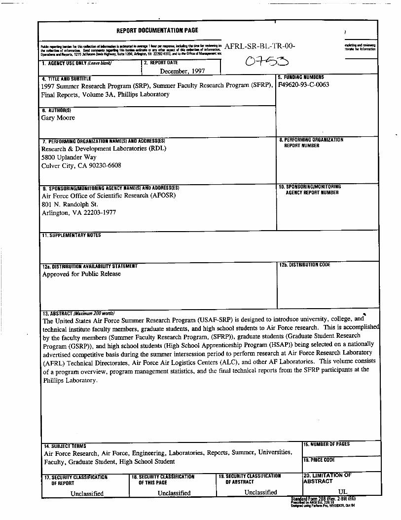
REPORT DOCUMENTATION PAGE
Pubfc reporting tata f« ttecohctkmrfinta!^ AFRL-SR-BL-TR-OO- the collection of infomntiai. Sand commits raganfing tut bunion estimate or ony other aspect of thii cohction of information. Operations and Reports. 1215 Jefferson Datis Highway. Suita 1204, Arlngton, VA 22202-4302, and to the Office of f>*
mpkrting and remvwig iterate for Informatian
1. AGENCY USE ONLY (Leave blank) 2. REPORT DATE
December, 1997 O^o^>
4. TITLE AND SUBTITLE 1997 Summer Research Program (SRP), Summer Faculty Research Program (SFRP), Final Reports, Volume 3A, Phillips Laboratory
6. AUTHOR(S)
Gary Moore
7. PERFORMING ORGANIZATION NAME(S) AND ADDRESS(ES)
Research & Development Laboratories (RDL) 5800 Uplander Way Culver City, CA 90230-6608
9. SPONSORING/MONITORING AGENCY NAME(S) AND ADDRESS(ES)
Air Force Office of Scientific Research (AFOSR) 801 N. Randolph St. Arlington, VA 22203-1977
5. FUNDING NUMBERS
F49620-93-C-0063
8. PERFORMING ORGANIZATION REPORT NUMBER
10. SPONSORING/MONITORING AGENCY REPORT NUMBER
11. SUPPLEMENTARY NOTES
12a. DISTRIBUTION AVAILABILITY STATEMENT
Approved for Public Release 12b. DISTRIBUTION CODE
13. ABSTRACT (Maximum 200 wonls) « The United States Air Force Summer Research Program (USAF-SRP) is designed to introduce university, college, and technical institute faculty members, graduate students, and high school students to Air Force research. This is accomplished by the faculty members (Summer Faculty Research Program, (SFRP)), graduate students (Graduate Student Research Program (GSRP)), and high school students (High School Apprenticeship Program (HSAP)) being selected on a nationally advertised competitive basis during the summer intersession period to perform research at Air Force Research Laboratory (AFRL) Technical Directorates, Air Force Air Logistics Centers (ALC), and other AF Laboratories. This volume consists of a program overview, program management statistics, and the final technical reports from the SFRP participants at the Phillips Laboratory.
14. SUBJECT TERMS Air Force Research, Air Force, Engineering, Laboratories, Reports, Summer, Universities, Faculty, Graduate Student, High School Student
17. SECURITY CLASSIFICATION OF REPORT
Unclassified
18. SECURITY CLASSIFICATION OF THIS PAGE
Unclassified
19. SECURITY CLASSIFICATION OF ABSTRACT
Unclassified
15. NUMBER OF PAGES
16. PRICE CODE
20. LIMITATION OF ABSTRACT
UL Standard Form 298 (Rev. 2-89) (EG) Prescribed by ANSI Std. 239.18 Designed using Perform Pro, WHSIDIOR. Oct 94
GENERAL INSTRUCTIONS FOR COMPLETING SF 298
The Report Documentation Page (RDP) is used in announcing and cataloging reports. It is important that this information be consistent with
the rest of the report, particularly the cover and title page. Instructions for filling in each block of the form follow. It is important to stay
within the lines to meet optical scanning requirements.
Block 1. Agency Use Only (Leave blank).
Block 2. Report Date. Full publication date including day, month, and year, if available (e.g. 1 Jan 88). Must cite at least the year.
Block 3. Type of Report and Dates Covered. State whether report is interim, final, etc. If applicable, enter inclusive report dates (e.g. 10Jun87-30Jun88).
Block 4. Title and Subtitle. A title is taken from the part of the report that provides the most meaningful and complete information. When a report is prepared in more than one volume, repeat the primary title, add volume number, and include subtitle for the specific volume. On classified documents enter the title classification in parentheses.
Block 5. Funding Numbers. To include contract and grant numbers; may include program element number(s), project number(s), task number(s), and work unit number(s). Use the following labels:
C - Contract G - Grant PE- Program
Element
PR - Project TA - Task WU - Work Unit
Accession No.
Block 6. Author(s). Name(s) of person(s) responsible for writing the report, performing the research, or credited with the content of the report. If editor or compiler, this should follow the name(s).
Block 7. Performing Organization Name(s) and Address(es). Self-explanatory.
Block 8. Performing Organization Report Number. Enter the unique alphanumeric report number(s) assigned by the organization performing the report.
Block 9. Sponsoring/Monitoring Agency Name(s) and Address(es). Self-explanatory.
Block 10. Sponsoring/Monitoring Agency Report Number. (If known)
Block 11. Supplementary Notes. Enter information not included elsewhere such as: Prepared in cooperation with....; Trans, of....; To be published in.... When a report is revised, include a statement whether the new report supersedes or supplements the older report.
Block 12a. Distribution/Availability Statement. Denotes public
availability or limitations. Cite any availability to the public. Enter
additional limitations or special markings in all capitals (e.g. NOFORN,
REL, ITAR).
DOD See DoDO 5230.24, "Distribution Statements on Technical Documents."
DOE See authorities. NASA See Handbook NHB 2200.2.
NTIS Leave blank.
ck 12b. Distribution Code.
DOD Leave blank. DOE Enter DOE distribution categories from the Stand
NASA
NTIS
Distribution for Unclassified Scientific and Technical
Reports.
Leave blank.
Leave blank.
Block 13. Abstract. Include a brief (Maximum 200 words) factual
summary of the most significant information contained in the report.
Block 14. Subject Terms. Keywords or phrases identifying major
subjects in the report.
Block 15. Number of Pages. Enter the total number of pages.
Block 16. Price Code. Enter appropriate price code (NTIS only).
Blocks 17.-19. Security Classifications. Self-explanatory. Enter
U.S. Security Classification in accordance with U.S. Security
Regulations (i.e., UNCLASSIFIED), if form contains classified
information, stamp classification on the top and bottom of the page.
Block 20. Limitation of Abstract. This block must be completed to
assign a limitation to the abstract. Enter either UL (unlimited) or SAR
(same as report). An entry in this block is necessary if the abstract is
to be limited. If blank, the abstract is assumed to be unlimited.
Standard Form 298 Back (Rev. 2-89]
SFRP FINAL REPORT TABLE OF CONTENTS i-xviii
1. INTRODUCTION 1
2. PARTICIPATION IN THE SUMMER RESEARCH PROGRAM 2
3. RECRUITING AND SELECTION 3
4. SITE VISITS 4
5. HBCU/MI PARTICIPATION 4
6. SRP FUNDING SOURCES 5
7. COMPENSATION FOR PARTICIPATIONS 5
8. CONTENTS OF THE 1996 REPORT 6
APPENDICIES:
A. PROGRAM STATISTICAL SUMMARY A-l
B. SRP EVALUATION RESPONSES B-l
SFRP FINAL REPORTS

PREFACE
Reports in this volume are numbered consecutively beginning with number 1. Each report is paginated with the report number followed by consecutive page numbers, e.g., 1-1, 1-2, 1-3; 2-1, 2-2, 2-3.
This document is one of a set of 16 volumes describing the 1997 AFOSR Summer Research Program. The following volumes comprise the set:
Due to its length, Volume 3 is bound in two parts, 3A and 3B. Volume 3A contains #1-18. Volume 3B contains reports #19-30. The Table of Contents for Volume 3 is included in both parts.
VOLUME
1
2A&2B
3A&3B
4A&4B
5A , 5B & 5C
6
7A&7B
10A & 10B
11
12A & 12B
13
14
15B&15B
16
TITLE
Program Management Report
Summer Faculty Research Program (SFRP) Reports
Armstrong Laboratory
Phillips Laboratory
Rome Laboratory
Wright Laboratory
Arnold Engineering Development Center, United States Air Force Academy and
Air Logistics Centers
Graduate Student Research Program (GSRP) Reports
Armstrong Laboratory
Phillips Laboratory
Rome Laboratory
Wright Laboratory
Arnold Engineering Development Center, United States Air Force
Academy, Wilford Hall Medical Center and Air Logistics Centers
High School Apprenticeship Program (HSAP) Reports
Armstrong Laboratory
Phillips Laboratory
Rome Laboratory
Wright Laboratory
Arnold Engineering Development Center

SRP Final Report Table of Contents
Author DR Jean M Andino
University/Institution Report Title
Armstrong Laboratory Directorate
AL/EQL university of Florida , Gainesville , FL Atmospheric Reactions of Volatille Paint Components a Modeling Approach
DR Anthony R Andrews Ohio University , Athens, OH
AL/EQL
Novel Electrochemiluminescence Reactions and Instrumentation
Vol-Page
2- 1
2- 2
DR Stephan B Bach AL/OEA Univ of Texas at San Antonio , San Antonio , TX Investigation of Sampling Interfaces for Portable Mass Spectormetry and a survery of field Portable
DR Marilyn Barger AL/EQL Florida A&M-FSU College of Engineering , Tallahassee , FL Analysis for The Anaerobic Metabolites of Toulene at Fire Training Area 23 Tyndall AFB, Florida
DR Dulal K Bhaumik AL/AOEP University of South Alabama , Mobile , AL The Net Effect of a Covariate in Analysis of Covariance
2- 3
2- 4
2- 5
DR Marc L Carter, PhD, PA Hofstra University , Hempstead , NY
AL/OEO
Assessment of the Reliability of Ground Based Observeres for the Detecton of Aircraft
2- 6
DR Huseyin M Cekirge AL/EQL Florida State University , Tallahassee , FL Developing a Relational Database for Natural Attenuation Field Data
2- 7
DR Cheng Cheng AL/HRM Johns Hopkins University , Baltimore , MD Investigation of Two Statistical Issues in Building a Classification System
2- 8
DR Gerald P Chubb AL/HR1 Ohio State University , Columbus, OH Use of Air Synthetic Forces For GCI Training Exercises
2- 9-
DR Sneed B Collard, Jr. AL/EQL University of West Florida , Pensacola , FL Suitability of Ascidians as Trace Metal Biosenosrs-Biomonitors In Marine Environments An Assessment
DR Catherine A Cornwell Svracuse University , Syracuse , NY
AL/OER
2- 10
2- 11
Rat Ultrasoud Vocalization Development and Neurochemistry in Stress-Sensitive Brain Regions

SRP Final Report Table of Contents
University/Institution Armstrong Laboratory AUthor Report Title Directorate Vol-Paa< DRBaolinDeng AL/EQL " JT-^
New Mexico Tech , Socorro , NM Effect of Iron Corrosion Inhibitors on Reductive Degradation of Chlorinated Solvents
DR Micheal P Dooley AL/OER . 2- 13 Iowa State University , Ames , IA
Copulatory Response Fertilizing Potential, and Sex Ratio of Offsprings Sired by male rats Ecposed
DRItielEDror AL/HRT 2 ^ Miami University , Oxford , OH
The Effect of Visual Similarity and Reference Frame Alignment on the Recognition of Military Aircraf
DR Brent D Foy AFRL/HES 2- 15 Wright State University , Dayton , OH Advances in Biologivcally-Based Kinetic Modeling for Toxicological Applications
DR IrwinS Goldberg AL/OES 2 ^ St. Mary's Univ , San Antonio , TX
Mixing and Streaming of a Fluid Near the Entrance of a Tube During Oscillatory Flow
DR Ramesh C Gupta ALOES 2 j?
University of Maine at Orono , Orono , ME A Dynamical system approach in Biomedical Research
DR John R Herbold AL/AOEL 2. 18
Univ of Texas at San Antonio , San Antonio , TX
A Protocol for Development of Amplicons for a Rapid and Efficient Methoiid of Genotypine Hepatitis C
DR Andrew E Jackson AL/HRA 2. 19
Arizona State University , Mesa , AZ
Development fo a Conceptual Design for an Information Systems Infrastructure To Support the Squadron
DR Charles E Lance AL/HRT ^ ^
Univ of Georgia Res Foundation , Athens , GA Replication and Extension of the Schmidt, Hunter, and Outerbridge (1986) Model of Job Performance R
DR David A Ludwig AL/AOCY 2. 21
Univ of N.C. at Greensboro , Greensboro , NC Mediating effect of onset rate on the relationship between+ Gz and LBNP Tolerance
DR Robert P Mahan AL/CFTO 2. 22
University of Georgia , Athens , GA
The Effects of Task Structure on Cognitive Organizing Principles Implaicatins for Complex Display v
11

SRP Final Report Table of Contents
University/Institution Armstrong Laboratory Author Report Title Directorate Voi-Page DR Phillip H Marshal! " AL/HRM 2- 23
Texas Tech University . Luhhock . TX Preliminary repon: on the effects of varieties of feedback training on single target time-to-contac
DR Bruce V Mutter AL/EQP 2- 24 Bluefield State College , Blucfield , WV
DR Allen L Nagy AL/CFHV 2- 25 Wright State University , Dayton . OH The Detection of Color Breakup In Field Sequential Color Displays
DR Brent L Nielsen AL/AOEL 2- 26 Auburn University , Auburn , AL Rapid PCR Detection of Vancomycin Resistance of Enteroccus Species in infected Urine and Blood
DR Thomas E Nygren AL/CFHP 2- 27 Ohio State University , Columbus , OH Group Differences in perceived importance of swat workload dimensions: Effects on judgment and perf
DR Edward H Piepmeier AL/AOHR 2- 28 Oregon State University , Corvallis, OR
DRJudyLRatliff AL/EQL 2- 29 Murray State Univ , Murray . KY Accumulation of Storntium and Calcium by Didemnum Conchyliatum
DR Joan R Rentsch AL/CFHI V 30 Wright State University , Dayton , OH the Effects of Individual Differences and Team Processed on Team Member Schema Similarity and task P
DR Paul D Retzlaff AL/AOCN 2- 31 Univ of Northern Colorado , Greelcy , CO The Armstrong Laboratory Aviation Personality Survey (ALAPS) Norming and Cross - Validation
DR David B Reynolds AL/CFBE 2- 32 Wright State University , Dayton , OH Modeling Heat Flux Through Fabrics Exposed to a Radiant Souurce and Analysis of Hot Air Burns
DR Barth F Smets AL/EQL 2- 33 University of Connecticut, Storrs , CT Desorption and Biodegradation of Dinitrotoluenes in aged soils
in
SRP Final Report Table of Contents
University/Institution Phillips Laboratory Author Report Title Directorate voi-Page DR Graham R Allan PL/LDDD 3- 1
National Avenue , Las Vegas , NM Temporal and Spatial Characterisation of a Synchronously-Pumped Periodically-Poled Lithium Niobate O
DR Mark J Balas PL/SX 3- 2 Univ of Colorado at Boulder, Boulder , CO Nonlinear Trackin« Control for a Precision Deployable Structure Using a Partitioned Filter Approach
DR Mikhail S Belen'kii PL/LIG 3- 3 Georgia Inst of Technology , Atlanta , GA Multiple Aperture Averaging Technique for Measurment Full Aperture Tilt with a Laser Guide Star and
DR Gajanan S Bhat PL/RK 3- 4 Univ of Tennessee , Knoxville , TN Spinning Hollow Fibers From High Performance Polymers
DR David B Choate PL/VTMR 3- 5 Transylvania Univ , Lexington , KY Blackhole Analysis
DR Neb Duric AFRL/DEB 3- 6 University of New Mexico , Albuquerque , NM Image Recovery Using Phase Diversity
DR Arthur B Edwards PL/VTMR 3- 7 9201 University City Blvd. , Charlotte , NC Theory of Protons in Buried Oxides
DR Gary M Erickson PL/GPSG 3- 8 Boston University , Boston , MA Modeling The Magnctospheric Magnetic Field
DR Hany A Ghoneim PL/RKES 3- 9 Rochester Inst of Technol, Rochester , NY Focal Point Accuracy Assessement of an Off-Axis Solar Caoncentrator
DRSubir Ghosh PL/RKBA 3- 10 Univ of Calif, Riverside . Riverside , CA Designing Propulsion Reliability of Space Launch Vehicles
DR George W Hanson AFRL/DEH 3- n Univ of Wisconsin - Milwaukee , Milwaukee , WI Asymptotic analysis of" the Natural system modes of coupled bodies in the large separatin, Low-Freque
iv
SRP Final Report Table of Contents
University/Institution Phillips Laboratory Author Report Title Directorate Vol-Page DR Brian D Jeffs AFRL/DES 3- 12
Brigham Young University , Pmvii, UT Blind Bayyesian Restoration of Adaptive Optics Images Using Generalized Gaussian Markov Random Field
DR Christopher H Jenkins PL/VTVS 3- 13 S Dakota School of Mines/Tech , Rapid City , SD Mechnics of Surface Precosion for Membrane Reflectors
DR Dikshitulu K Kalluri PL/GPID 3- 14 University of Lowell, Lowell, MA Mode Conversion in a Time-Varying Magnetoplasma Medium
DRAravindaKar AFRL/DEO 3- 15 University of Central Florida , Orlando , FL Measurement of the Cutting Performance of a High Beam Quality Chemical Oxygen-Iodine Laser on Aerosp
DR Bernard Kirtman PL/VTMR 3- 16 Univ of Calif, Santa Barbara , Santa Barbara , CA Quantum Chemical Characterization of the elkectronic Structure and Reactions of Silicon Dangling Bon
DR Spencer P Kuo PL.GPI 3- 17 Polytechnic University , Fanningdale , NY Excitation of Oscillating Two Stream Instability by Upper Hybrid Pump Waves in Ionospheric Heating
DR Henry A Kurtz PL/VTMR 3- 18 Memphis State University , Memphis , TN H2 Reactions at Dangling Bonds in SI02
DR Min-Chang Lee PL/GPSG 3- 19 Massachusetts Inst of Technology , Cambridge , MA Laboratory Studies of Ionospheric Plasma Effects Produced by Lightning-induced Whistler Waves
DR Donald J Leo AFRL/VSD 3- 20 University of Toledo , Toledo , OH Microcontroller-Based Implementation of Adaptive Structural Control
DRHuaLi PL/LIDD 3- 21 University of New Mexico , Albuquerque , NM
DR Hanli Liu AFRL/DEB 3- 22 Univ of Texas at Arlington , Arlington , TX Experimental Validation of Three-Dimensional Reconstruction of Inhomogenety Images in Turbid Media
SRP Final Report Table of Contents
University/Institution Phillips Laboratory Author Report Title Directorate voi-Page DR M. Arfin K Lodhi PL/VTRP _ 3- 23
Texas Tech University , Luhhock , TX Thermoelectric Energy Conversion with solid Electolytes
DR Tim C Newell PL/LIGR 3- 24 University of New Mexico , Albuquerque , NM Study of Nonlineaar Dynamics in a Diode Pumped Nd:YAG laser
DR MichaelJ Pangia PL/GPSG 3- 25 Georgia College & State University , Millcdgeville , GA Preparatory Work Towards a Computer Simulation of Electron beam Operations on TSS 1
DR Vladimir O Papitashvili PL/GPSG 3- 26 Univ of Michigan , Ann Arbor , MI Modeling of Ionospheric Convectin from the IMF and Solar Wind Data
DR Jaime Ramirez-Angulo PL/VTMR 3- 27 New Mexico State University , Las Cruces , NM
DR Louis F Rossi PL/GPOL 3- 28 University of Lowell, Lowell, MA Analysis of Turbulent Mixing in the Stratosphere & Troposphere
DR David P Stapleton PL/RKBA 3- 29 University of Central Oklahoma , Edmond , OK Atmospheric Effects Upon Sub-Orbital Boost glide Spaceplane Trajectories
DR Jenn-Ming Yang PL/RKS 3- 30 Univ of Calif, Los Angeles , Los Angeles , CA Thermodynamic Stability and Oxidation Behavior of Refractory (Hf, Ta, Zr) Carbide/boride Composites
VI
SRP Final Report Table of Contents
University/Institution Rome Laboratory Author Report Title Directorate Vol-Page DR A. F Anwar RL/ERAC 4- 1
University of Connecticut, Storrs , CT Properties of Quantum Wells Formed In AIGaN/GaN Heternstructures
DR Milica Barjaktarovic AFRL/IFG ____ 4- 2 Wilkes University , Wilkes Barre , PA Assured Software Design: Privacy Enhanced Mail (PEM) and X.509 Certificate Specification
DR Stella N Batalama AFRL/IFG __ 4- 3 SUNY Buffalo , Buffalo , NY Adaptive Robust Spread-Spectrum Receivers
DR Adam W Bojanczyk RL/OCSS 4- 4 Cornell Univesity , Ithaca , NY Lowering the Computational Complexity of Stap Radar Systems
DR Nazeih M Botros RL/ERC-1 4- 5 So. Illinois Univ-Carbondale , Carbondale , IL A PC-Based Speech Synthesizing Using Sinusoidal Transform Coding (STC)
DR Nikolaos G Bourbakis AFRL/IF 4- 6 SUNY Binghamton, Binghamton , NY Eikones-An Object-Oriented Language Forimage Analysis & Process
DR Peter P Chen RL/CA-H 4- 7 Louisiana State University , Baton Rouge , LA Reconstructing the information Warfare Attack Scenario Guessing what Actually Had Happened Based on
DR Everett E Crisman RL/ERAC 4- 8 Brown University , Providence , RI A Three-Dimensional, Dielectric Antenna Array Re-Configurable By Optical Wavelength Multiplexing
DR Digendra K Das RL/ERSR 4- 9 SUNYIT , Utica , NY A Study of the Emerging Dianostic Techniques in Avionics
DR Venugopala R Dasigi AFRL/IFT 4- 10 Southern Polytechnic State Univ , Marietta , GA Information Fusion for text Classification-an Expjerimental Comparison
DR Richard R Eckert AFRL/IFSA 4- n SUNY Binghamton , Binghamton , NY Enhancing the rome Lab ADÜ virtual environment system
vii
SRP Final Report Table of Contents
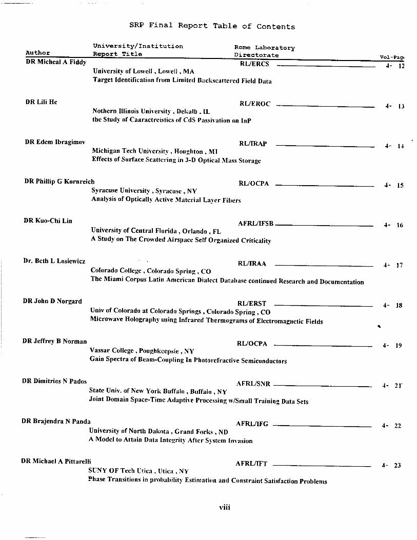
University/Institution Rome Laboratory Author Report Title Directorate voi-pag, DR Micheal A Fiddy " Ri/rnrs — J—^
University of Lowell, Lowell, MA Target Identification from Limited Backscattered Field Data
DR Lili He RL/EROC Nothern Illinois University , Dekali), IL the Study of Caaractreistics of CdS Passivation on InP
DR Edem Ibragimov RL/IRAP Michigan Tech University , Houghton , MI Effects of Surface Scattering in 3-D Optical Mass Storage
4- 13
4- 14
DR Phillip G Kornreich RL/OCPA 4. 15
Syracuse University , Syracuse , NY Analysis of Optically Active Material Layer Fibers
DRKuo-ChiLin AFRL/IFSB- 4. 16
University of Central Florida , Orlando , FL A Study on The Crowded Airspace Self Organized Criticality
Dr. Beth L Losiewicz RL/IRAA 4- 17
Colorado College , Colorado Spring , CO The Miami Corpus Latin American Dialect Database continued Research and Documentation
DR John D Norgard RL/ERST Univ of Colorado at Colorado Springs , Colorado Spring , CO Microwave Holography using Infrared Thermograms of Electromagnetic Fields
4- 18
DR Jeffrey B Norman RL/OCPA - 4- 19
Vassar College , Poughkeepsie , NY Gain Spectra of Beam-Coupling In Photorefractive Semiconductors
DR Dimitrios N Pados AFRL/SNR State Univ. of New York Buffalo , Buffalo , NY Joint Domain Space-Time Adaptive Processing w/Small Training Data Sets
DR Brajendra N Panda AFRL/IFG University of North Dakota , Grand Forks , ND A Model to Attain Data Integrity After Svstem Invasion
4- 21'
4- 22
DR Michael A Pittarelli AFRL/IFT 4- ?3 SUNY OF Tech Utica , Utica , NY Phase Transitions in probability Estimation and Constraint Satisfaction Problems
vin

SRP Final Report Table of Contents
University/Institution Rome Laboratory Author Report Title Directorate Vol-Page DR Salahuddin Qazi RL/IWT 4- 24
SUNY OF Tech Utica , Utica , NY Low Data rate Multimedia Communication Using Wireless Links
DR Arindam Saha RL/OCSS 4- 25 Mississippi State University , Mississippi State , MS An Implementation;! of the message passing Interface on Rtems
, DRRaviSankar RL/C3BC 4- 26 University of South Florida , Tampa , FL A Study oflntegrated and Intelligent Network Management
DR Mark S Schmalz AFRL/IF 4- 27 University of Florida , Gainesville , FL Errors inherent in Reconstruction of Targets From multi-Look Imagery
DR John L Stensby RL/IRAP 4- 28 Univ of Alabama at Huntsville , Huntsville , AL Simple Real-time Tracking Indicator for a Frequrncy Feedback Demodulator
DR Micheal C Stinson . RL/CAU 4- 29 Central Michigan University , Mt. Pleasant, MI Destructive Objects
DR Donald R Ucci RL/C3BB 4- 30 Illinois Inst of Technology , Chicago , IL Simulation of a Robust Locally Optimum Receiver in correlated Noise Using Autoregressive Modeling *
DRNongYe AFRL/IFSA 4- 31 Arizona State University , Tcmpe , AZ A Process Engineering Approach to Continuous Command and Control on Security-Aware Computer Networks
IX
SRP Final Report Table of Contents
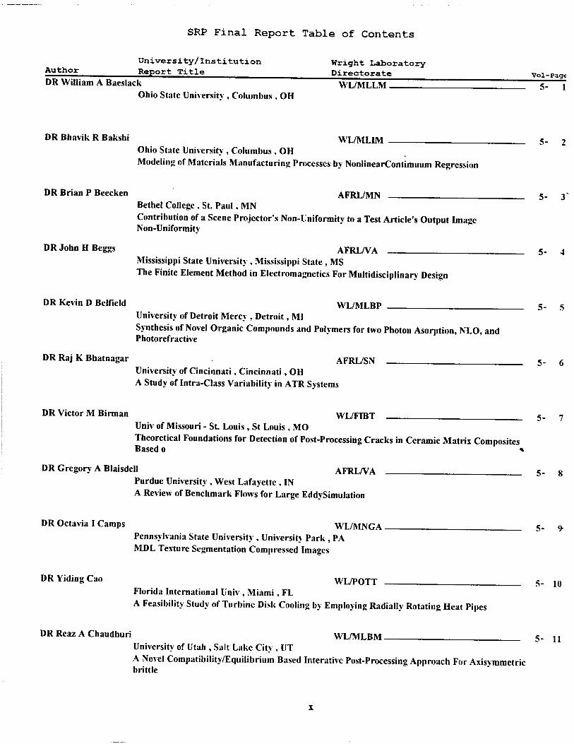
University/Institution Wright Laboratory Author Report Title Directorate Vol.Pagt
DR William A Baeslack WL/MLLM ___ 5- 1 Ohio State University , Columbus , OH
DR Bhavik R Bakshi WL/MLBM 5- 2 Ohio State University , Columbus , OH Modeling of Materials Manufacturing Processes by NonlinearContimuum Regression
DR Brian P Beecken AFRL/MN 5. 3' Bethel College , St. Paul, MN Contribution of a Scene Projector's Non-Uniformity to a Test Article's Output Image Non-Uniformity
DRJohnHBeggs AFRL/VA 5- 4 Mississippi State University , Mississippi State , MS The Finite Element Method in Electromagnetics For Multidisciplinary Design
DR Kevin D Belfield WL/MLBP . 5- 5 University of Detroit Mercy , Detroit, MI Synthesis of Novel Organic Compounds and Polymers for two Photon Asorption, NLO, and Photorefractive
DR Raj K Bhatnagar AFRL/SN 5- 6
University of Cincinnati, Cincinnati, OH A Study of Intra-Class Variability in ATR Systems
DR Victor M Birman WL/FIBT 5- 7 Univ of Missouri - St. Louis , St Louis , MO Theoretical Foundations for Detection of Post-Processing Cracks in Ceramic Matrix Composites Based 0 *
DR Gregory A Blaisdell AFRL/VA 5- g Purdue University , West Lafayette , IN A Review of Benchmark Flows for Large EddySimulation
DR Octavia I Camps WL/MNGA 5- * Pennsylvania State University , University Park , PA MDL Texture Segmentation Compressed Images
DRYidingCao WL/POTT 5- 10 Florida International Univ , Miami, FL A Feasibility Study of Turbine Disk Cooling by Employing Radially Rotating Heat Pipes
DR Reaz A Chaudhuri WL/MLBM 5- n University of Utah , Salt Lake City , UT
A Novel Compatibility/Equilibrium Based Interative Post-Processing Approach For Axisymmetric brittle
SRP Final Report Table of Contents
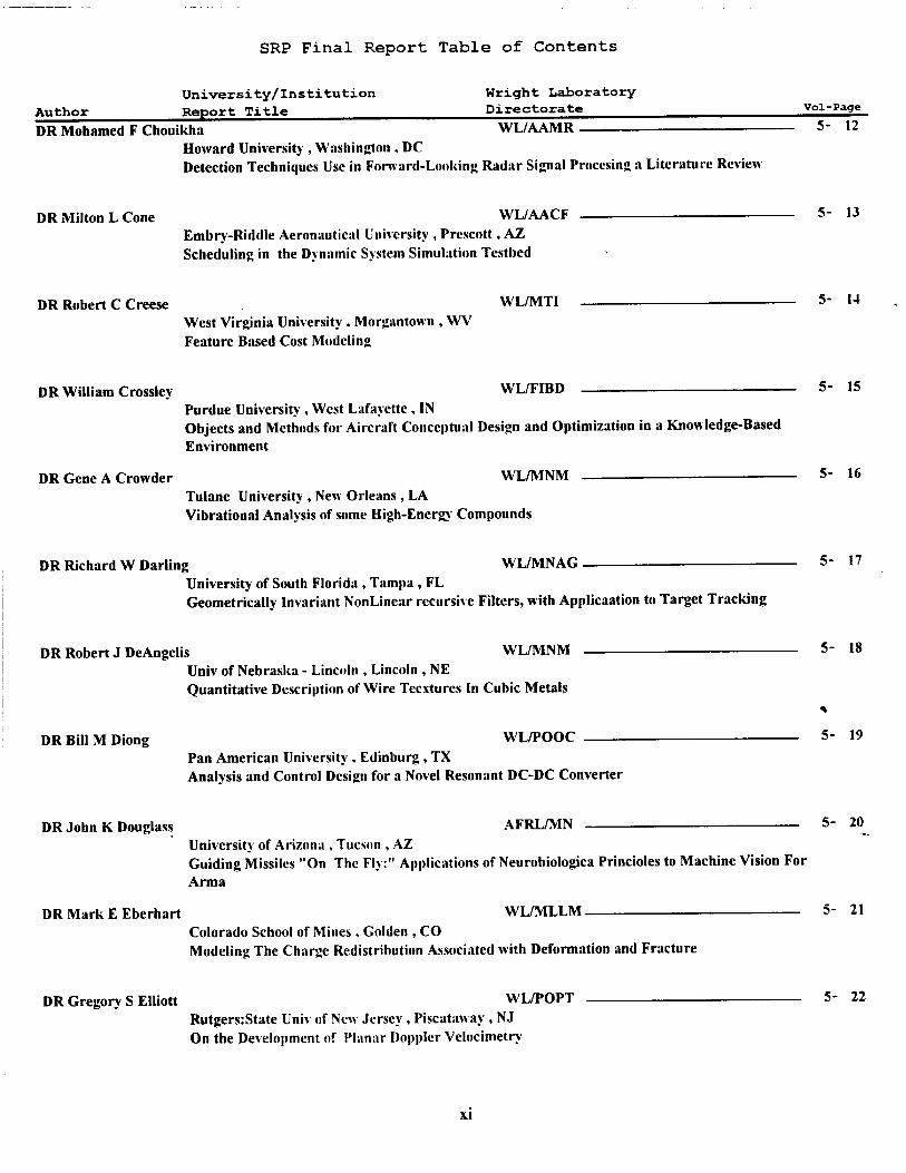
University/Institution Wright Laboratory Author Report Title Directorate voi-Page DR Mohamed F Chouikha WL/AAMR 5- 12
Howard University , Washington , DC Detection Techniques Use in Forward-Looking Radar Signal Proccsing a Literature Review
DR Milton L Cone WL/AACF _ 5- 13 Embry-Riddle Aeronautical University , Prescott, AZ Scheduling in the Dynamic System Simulation Testbed
DR Robert C Creese WL/MTI 5- 14 West Virginia University , Morgantown , WV Feature Based Cost Modeling
DR William Crossley WL/FIBD 5- 15 Purdue University , West Lafayette , IN Objects and Methods for Aircraft Conceptual Design and Optimization in a Knowledge-Based Environment
DR Gene A Crowder WL/MNM _ 5- 16 Tulane University , New Orleans , LA Vibrational Analysis of some High-Energy Compounds
DR Richard W Darling WL/MNAG — 5- 17 University of South Florida , Tampa , FL Geometrically Invariant NonLinear recursive Filters, with Applicaation to Target Tracking
DR Robert J DeAngelis WL/MNM 5- 18 Univ of Nebraska - Lincoln , Lincoln , NE Quantitative Description of Wire Tecxtures In Cubic Metals
DR Bill M Diong WL/POOC — 5- 19 Pan American University , Edinburg, TX Analysis and Control Design for a Novel Resonant DC-DC Converter
DR John K Douglass AFRL/MN 5- 20 University of Arizona , Tucson , AZ Guiding Missiles "On The Fly:" Applications of Neurobiologica Princioles to Machine Vision For Arma
DR Mark E Eberhart WL/MLLM 5- 21 Colorado School of Mines , Golden , CO Modeling The Charge Redistribution Associated with Deformation and Fracture
DR Gregory S Elliott WL/POPT 5- 22 Rutgers:State Univ of New Jersey , Piscataway , NJ On the Development of Planar Dopplcr Velocimetry
XI

University/Institution Wright Laboratory Author Report Title Directorate Vol-Pagt DR Elizabeth A Ervin WL/POTT 5- 23
University of Dayton , Dayton , OH Eval of the Pointwise K-2 Turbulence Model to Predict Transition & Scpartion in a Low Pressure
DR Altan M Ferendeci WL/AADI 5- 24 University of Cincinnati, Cincinnati, OH Vertically Interconnected 3D MMICs with Active Interlayer Elements
DR Dennis R Flentge WL/POSL 5- 25 Cedarville College , Cedarville , OH Kinetic Study of the Thermal Decomposition of t-Butylphenyl Phosphate Using the System for Thermal D
DR George N Frantziskonis WL/MLLP 5- 26 University of Arizona , Tuson , AZ Multiscale Material Characterization and Applications
DR Zewdu Gebeyehu WL/MLPO 5- 27 Tuskegee University , Tuskegee , AL Synthesis and Characterization of Metal-Xanthic Acid and -Amino Acid Comdexes Useful Ad Nonlinear
DR Richard D Gould WL/POPT 5- 28 North Carolina State U-Raleigh , Raleigh , NC Reduction and Analysis of LDV and Analog Raw Data
DR Michael S Grace WL/MLPJ 5- 29 University of Virginia , Charlottesville , VA Structure and Function of an Extremely Sensitive Biological Infrared Detector
DR Gary M Graham WL/FIGC 5- 30 Ohio University , Athens , OH Indicia! Response Model for Roll Rate Effects on A 65-Degree Delta wing
DR Allen G Greenwood WL/MTI 5- 31 Mississippi State University , Mississippi Sta , MS An Object-Based approach for Integrating Cost Assessment into Product/Process Design
DR Rita A Gregory WL/FFVC 5- 32 Georgia Inst of Technology , Atlanta , GA Range Estimating for Research and Development Alternatives
DR Mark T Hanson WL/MNM 5- 33 University of Kentucky , Lexington , KY Anisotropy in Epic 96&97: Implementation and Effects
Xll

SRP Final Report Table of Contents
University/Institution Wright Laboratory Author Report Title Directorate Voi-Page DR Majeed M Hayat WL/AAJT 5- 34
University of Dayton , Dayton , OH A Model for Turbulence and Photodctcction Noise in Imaging
DR Larry S Heimick WL/MLBT 5- 35 Cedarvillc College , Cedarvillc , OH NMA Study of the Decomposition Reaction Path of Demnum fluid under Tribological Conditions
DR William F Hosford AFRL/MN 5- 36 Univ of Michigan , Ann Arbor , MI INTENSITY OF [111JAND [100) TEXTURAL COMPONENTS IN COMPRESSION-FORGED TANTALUM
DR David E Hudak WL/FIMC 5- 37 Ohio Northern University , Ada , OH A Study fo a Data-Parallel Imlementation of An Implicit Solution fo the 3D Navier-Stokes Equations
DR David P Johnson WL/MNAZ 5- 38 Mississippi State University , Mississippi, MS An Innovative Segmented Tugsten Penetrating Munition
DR Ismail I Jouny WL/AACT 5- 39 Lafayette College , Easton , PA
DR Edward T Knobbe WL/MLBT 5- 40 Oklahoma State University , Stilhvater, OK Organically Modified silicate Films as Corrosion Resistant Treatments for 2024-T3 AJumium Alloy ,
DRSeungugKoh WL/AAST 5- 41 University of Dayton , Dayton , OH Numerically Efficinet Direct Ray Tracing Algorithms for Automatic Target Recognition using FPGAs
DR Ravi Kothari WL/AACA 5- 42.. University of Cincinnati, Cincinnati, OH A Function Approximation Approach for Region of Interest Selection in synthetic Aperture Radar Image
DR Douglas A Lawrence WL/MNAG 5- 43 Ohio University , Athens , OH On the Analysis and Design of Gain scheduled missile Autopilots
DR Robert Lee WL/FIM 5- 44 Ohio State University , Columbus, OH Boundary Conditions applied to the Finite Vlume Time Domain Method for the Solution of Maxwell's Equ
Xlll

SRP Final Report Table of Contents
University/Institution Wright Laboratory Author Report Title Directorate DR Junghsen Lieh WL/FIV
Wright State University , Dayton , OH Develop an Explosive Simulated Testing Apparatus for Impact Physics Research at Wright Laboratory
DR James S Marsh WL/MNSI University of West Florida , Pensacola , FL Distortion Compensation and Elimination in Holographic Reocnstruction
DR Richard O Mines WLMN/M University of South Florida , Tampa , FL Testing Protocol for the Demilitarization System at the Eglin AFB Herd Facility
DR Dakshina V Murty t WL/FIBT University of Portland , Portland , OR A Useful Benchmarking Method in Computational Mechanics, CFD, adn Heat Tansfcr
Vol-Page 5- 45
5- 46
DR Mark D McClain WL/MLBP 5- 47 Cedarville College , Cedarville , OH A Molecular Orbital Theory Analysis of Oligomers of 2,2'-Bithiazole and Partially Reduced 3,3'-Dimet
DR William S McCormick WL/AACR 5. 4g Wright State University , Dayton , OH Some Observations of Target Recognition Using High Range Resolution Radar
5- 49
5- 50
DR Krishna Naishadham WL/MLPO 5- 51 Wright State University , Dayton , OH
DR Serguei Ostapenko WL/MLPO 5- 52 University of South Florida , Tampa , FL
5- 53.. DRYiPan AFRL/VA _
University of Dayton , Dayton , OH Improvement of Cache Utilization and Parallel Efficiency of a Time-Dependnet Maxwell Equation Solver
DR Rolfe G Petschek WL/MLPJ 5- 54 Case Western Reserve Univ , Cleveland , OH AB INITIO AUANTUM CHEMICAL STUDIES OF NICKEL DITHIOLENE COMPLEX
DR Kishore V Pochiraju AFRL/ML 5- 55 Stevens Inst of Technology , Hoboken , NJ Refined Reissner's Variational Solution in the Vicinity of Stress Singularities
xiv
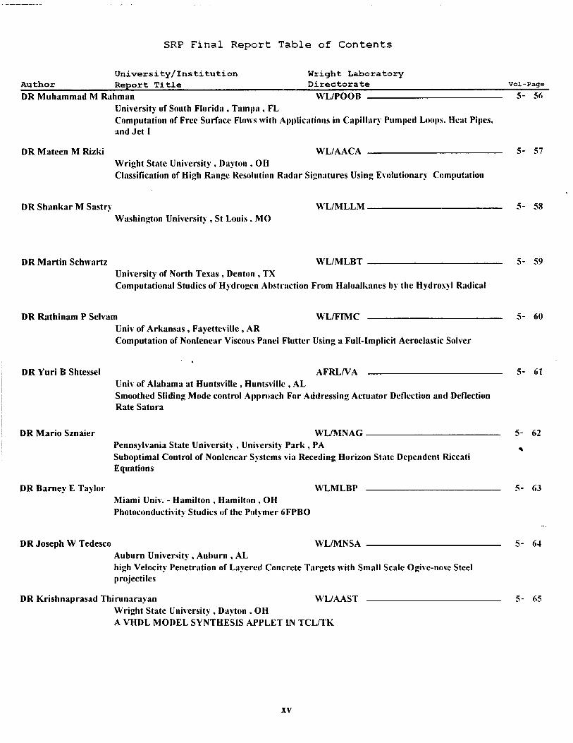
SRP Final Report Table of Contents
University/Institution Wright Laboratory Author Report Title Directorate vol-Page
DR Muhammad M Rahman WL/POOB 5- 56 University of South Florida , Tampa , FL Computation of Free Surface Flows with Applications in Capillary Pumped Loops. Heat Pipes, and Jet I
DR Mateen M Rizki WL/AACA 5- 57 Wright State University , Dayton . OH Classification of High Range Resolution Radar Signatures Using Evolutionary Computation
DR Shankar M Sastry WL/MLLM 5- 58 Washington University , St Louis . MO
DR Martin Schwartz WL/MLBT 5- 59 University of North Texas , Denton , TX Computational Studies of Hydrogen Abstraction From Haloalkanes by the Hydroxyl Radical
DR Rathinam P Selvam WL/FIMC 5- 60 Univ of Arkansas , Fayetteville , AR Computation of Nonlenear Viscous Panel Flutter Using a Full-Implicit Aeroelastic Solver
DR Yuri B Shtessel AFRL/VA 5- 61 Univ of Alabama at Huntsville , Huntsville , AL Smoothed Sliding Mode control Approach For Addressing Actuator Deflection and Deflection Rate Satura
DR Mario Sznaier WL/MNAG 5- 62
* Pennsylvania State University , University Park , PA Suboptimal Control of Nonlenear Systems via Receding Horizon State Dependent Riccati Equations
DR Barney E Taylor WLMLBP 5- 63 Miami Univ. - Hamilton , Hamilton , OH Photoconductivity Studies of the Polymer 6FPBO
DR Joseph W Tedesco WL/MNSA 5- 64 Auburn University , Auburn , AL high Velocity Penetration of Layered Concrete Targets with Small Scale Ogive-nose Steel projectiles
DR Krishnaprasad Thirunarayan WL/AAST 5- 65 Wright State University , Dayton , OH A VHDL MODEL SYNTHESIS APPLET IN TCL/TK
xv
SRP Final Report Table of Contents
University/Institution Wright Laboratory Author Report Title Directorate vol-Page DR Karen A Tomko WL/FIMC _ 5- 66
Wright State University , Dayton , OH Grid Level Parallclization of an Implicit Solution of the 3D Navier-Stokcs Equations
DR Max B Trueblood WL/POSC 5- 67 University of Missouri-Rolla , Rolla , MO AStudy of the Particulate Emissions of a Well-Stirred Reactor
DR Chi-Tay Tsai WL/AA 5- 68 Florida Atlantic University , Boca Raton , FL Dislocation Dynamics in Heterojunction Bipolar Transistor Under Current Induced Thermal St
DRJohnLValasek WL/FIMT 5- 69 Texas A&M University , College Station , TX Two Axis Pneumatic Vortex Control at High Speed and Low Angle-of-Attack
DR Mitch J Wolff WL/POTF 5- 70 Wright State University , Dayton , OH An Experimaental and Computational Analysis of the Unsteady Blade Row Potential Interaction inaTr
DR Rama K Yedavalli . WL/FIBD 5- 71 Ohio State University , Columbus , OH Improved Aircraft Roll Maneuver Performance Using Smart Deformable Wings
XVI
University/Institution Arnold Engineering Development Center Author Report Title Directorate Vol-Page DRCsabaABiegl AEDC/SVT 6- 1
Vanderbilt University , Nashville , TN Parallel processing for Tubine Engine Modeling and Test Data validation
DR Frank G Collins AEDC _ 6- 2 Tennessee Univ Space Institute , Tullahoma , TN Design of a Mass Spectrometer Sampling Probe for The AEDC Impulse Facility
DR Kenneth M Jones AEDC/SVT 6- 3 N Carolina A&T State Univ , Greensboro , NC
DR Kevin M Lyons AEDC/SVT 6- 4 North Carolina State U-Raleigh , Raleigh , NC Velocity Field Measurements Using Filtercd-Raylcigh Scattering
DR Gerald J Micklow AEDC/SVT 6- 5 Univ of Alabama at Tuscaloosa , Tucasloosa , AL
DR Michael S Moore AEDC/SVT 6- 6 Vanderbilt University , Nashville , TN Extension and Installation of the Model-Integrated Real-Time Imaging System (Mirtis)
DR Robert L Roach AEDC 6- 7 Tennessee Univ Space Institute , Tullahoma , TN Investigation of Fluid Mechanical Phenomena Relating to Air Injection Between the Segments of an Arc
DR Nicholas S Winowich AEDC <- 8 University of Tennessee , Knoxville , TN
DR Daniel M Knauss USAFA/DF 6- 9 Colorado School of Mines , Golden , CO Synthesis of salts With Delocalized Anions For Use as Third Order Nonlinear Optical Materials
DR Jeffrey M Bigelow OCALC/TI 6- 10 Oklahoma Christian Univ of Science & Art, Oklahoma City , OK Raster-To-Vector Conversion of Circuit Diagrams: Software Requirements
XVII
SRP Final Report Table of Contents
Author University/Institution Report Title
Arnold Engineering Development Center Directorate Vol-Page
DR Paul W Whaley OCALC/L Oklahoma Christian Univ of Science & Art, Oklahoma City , OK A Probabilistic framework for the Analysis of corrosion Damage in Aging Aircraft
6- II
DR Bjong W Yeigh OCALC/TI Oklahoma State University , Stilbvater , OK Logistics Asset Management: Models and Simulations
6- 12
DR Michael J McFarland Utah State University , Logan , UT
OC-ALC/E
Delisting of Hill Air Force Base's Industrial Wastewater Treatment Plant Sludge
6- 13
DR William E Sanford OO-ALC/E Colorado State University , Fort Collins , CO Nuerical Modeling of Physical Constraints on in-SItu Cosolvent Flushing as a Groundwate*. Remedial Op
DR Sophia Hassiotis University of South Florida , Tampa , FL Fracture Analysis of the F-5,15%-Spar Bolt
SAALC/TI
6- 14
6- 15
DR Devendra Kumar SAALC/LD CUNY-City College , New York , NY A Simple, Multiversion Concurrency Control Protocol For Internet Databases
6- 16
DR Ernest L McDuffie SAALC/TI Florida State University , Tallahassee , FL A Propossed Exjpert System for ATS Capability Analysis
6- 17
DR Prabhaker Mateti SMALC/TI Wright State University , Dayton , OH How to Provide and Evaluate Computer Network Security
6- 18
DR Mansur Rastani SMALC/L N Carolina A&T State Univ , Greensboro , NC Optimal Structural Design of Modular Composite bare base Shelters
6- 19
DR Joe G Chow WRALC/TI Florida International Univ , Miami, FL Re-engineer and Re-Manufacture Aircraft Sstructural Components Using Laser Scannii
6- 20
XVI11
1. INTRODUCTION
The Summer Research Prosram (SRP), sponsored by the Air Force Office of Scientific Research (AFOSR), offers paid opportunities for university faculty, graduate students, and high school students to conduct research in U.S. Air Force research laboratories nationwide during the summer.
Introduced by AFOSR in 1978, this innovative program is based on the concept of teaming academic researchers with Air Force scientists in the same disciplines using laboratory facilities and equipment not often available at associates' institutions.
The Summer Faculty Research Program (SFRP) is open annually to approximately 150 faculty members with at least two years of teaching and/or research experience in accredited U.S. colleges, universities, or technical institutions. SFRP associates must be either U.S. citizens or permanent
residents.
The Graduate Student Research Program (GSRP) is open annually to approximately 100 graduate students holding a bachelor's or a master's degree; GSRP associates must be U.S. citizens enrolled full
time at an accredited institution.
The High School Apprentice Program (HSAP) annually selects about 125 high school students located within a twenty mile commuting distance of participating Air Force laboratories.
AFOSR also offers its research associates an opportunity, under the Summer Research Extension Program (SREP), to continue their AFOSR-sponsored research at their home institutions through the award of research grants. In 1994 the maximum amount of each grant was increased from $20,000 to $25,000, and the number of AFOSR-sponsored grants decreased from 75 to 60. A separate annual
report is compiled on the SREP.
The numbers of projected summer research participants in each of the three categories and SREP "grants" are usually increased through direct sponsorship by participating laboratories.
AFOSR's SRP has well served its objectives of building critical links between Air Force research laboratories and the academic community, opening avenues of communications and forging new research relationships between Air Force and academic technical experts in areas of national interest, and strengthening the nation's efforts to sustain careers in science and engineering. The success of the SRP can be gauged from its growth from inception (see Table 1) and from the favorable responses the 1997 participants expressed in end-of-tour SRP evaluations (Appendix B).
AFOSR contracts for administration of the SRP by civilian contractors. The contract was first awarded to Research & Development Laboratories (RDL) in September 1990. After completion of the
1990 contract. RDL (in 1993) won the recompetition for the basic year and four 1-year options.
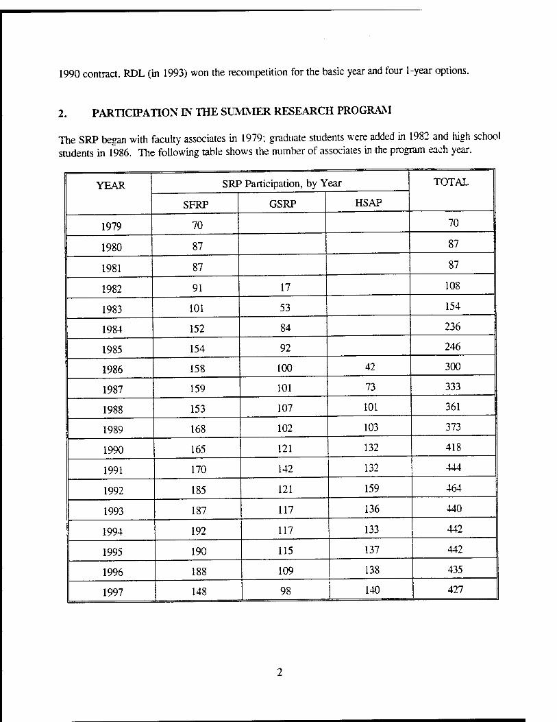
2. PARTICIPATION IN THE SUMMER RESEARCH PROGRAM
The SRP began with faculty associates in 1979; graduate students were added in 1982 and high school students in 1986. The following table shows the number of associates in the program each year.
YEAR SRP Participation, by Year TOTAL
SFRP GSRP HSAP
1979 70 70
1980 87 87
1981 87 87
1982 91 17 108
1983 101 53 154
1984 152 84 236
1985 154 92 246
1986 158 100 42 300
1987 159 101 73 333
1988 153 107 101 361
1989 168 102 103 373
1990 165 121 132 418
1991 170 142 132 444
1992 185 121 159 464
1993 187 117 136 440
1994 192 117 133 442
1995 190 115 137 442
1996 188 109 138 435
1997 148 98 140 427
Beginning in 1993. due to budget cuts, some of the laboratories weren't able to afford to fund as many associates as in previous years. Since then, the number of funded positions has remained fairly
constant at a slightly lower level.
3. RECRUITING AND SELECTION
The SRP is conducted on a nationally advertised and competitive-selection basis. The advertising for faculty and graduate students consisted primarily of the mailing of 8,000 52-page SRP brochures to chairpersons of departments relevant to AFOSR research and to administrators of grants in accredited universities, colleaes, and technical institutions. Historically Black Colleges and Universities (HBCUs) and Minority Institutions (Mis) were included. Brochures also went to all participating USAF laboratories, the previous year's participants, and numerous individual requesters (over 1000
annually).
RDL placed advertisements in the following publications: Black Issues in Higlier Education, Winds of Orange, and IEEE Spectrum. Because no participants list either Physics Today or Chemical & Engineering News as being their source of learning about the program for the past several years, advertisements in these magazines were dropped, and the funds were used to cover increases in
brochure printing costs.
High school applicants can participate only in laboratories located no more than 20 miles from their residence. Tailored brochures on the HSAP were sent to the head counselors of 180 high schools in the vicinity of participating laboratories, with instructions for publicizing the program in their schools. High school students selected to serve at Wright Laboratory's Armament Directorate (Eglin Air Force
Base, Florida) serve eleven weeks as opposed to the eight weeks normally worked by high school students at all other participating laboratories.
Each SFRP or GSRP applicant is given a first, second, and third choice of laboratory. High school students who have more than one laboratory or directorate near their homes are also given first,
second, and third choices.
Laboratories make their selections and prioritize their nominees. AFOSR then determines the number to be funded at each laboratory and approves laboratories' selections.
Subsequently, laboratories use their own funds to sponsor additional candidates. Some selectees do not accept the appointment, so alternate candidates are chosen. This multi-step selection procedure results in some candidates being notified of their acceptance after scheduled deadlines. The total applicants and participants for 1997 are shown in this table.

PARTICIPANT CATEGORY
SFRP
(HBCU/MD GSRP
(HBCU/MD
HSAP
TOTAL
199" Applicants and Participants
TOTAL APPLICANTS
490
(0) 202
(0)
433
1125
SELECTEES
1SS
(0 . 9S
(0)
140
426
DECLINING SELECTEES
(0)
(0)
14
55
4. SITE VISITS
Durina June and July of 1997, representatives of both AFOSR/NI and RDL visited each participating laboratory to provide briefings, answer questions, and resolve problems for both laboratory personnel and participants. The objective was to ensure that the SRP would be as constructive as possible for all participants. Both SRP participants and RDL representatives found these visits beneficial. At many of the laboratories, this was the only opportunity for all participants to meet at one time to share their experiences and exchange ideas.
5. HISTORICALLY BLACK COLLEGES AND UNIVERSITIES AND MINORITY INSTITUTIONS (HBCU/Mb)
Before 1993, an RDL program representative visited from seven to ten different HBCU/MIs annually to promote interest in the SRP among the faculty and graduate students. These efforts were marginally effective, yielding a doubling of HBCI/MI applicants. In an effort to achieve AFOSR's goal of 10% of all applicants and selectees being HBCU/NH qualified, the RDL team decided to try other avenues of approach to increase the number of qualified applicants. Through the combined efforts of the AFOSR Program Office at Boiling AFB and RDL, two very active minority groups were found, HACU (Hispanic American Colleges and Universities) and AISES (American Indian Science and Engineering Society). RDL is in communication with representatives of each of these organizations on a monthly basis to keep up with the their activities and special events. Both organizations have widely-distributed magazines/quarterlies in which RDL placed ads.
Since 1994 the number of both SFRP and GSRP HBCU/MI applicants and participants has increased ten-fold, from about two dozen SFRP applicants and a half dozen selectees to over 100 applicants and two dozen selectees, and a half-dozen GSRP applicants and two or three selectees to 18 applicants and 7 or 8 selectees. Since 1993, the SFRP had a two-fold applicant increase and a two-fold selectee increase. Since 1993, the GSRP had a three-fold applicant increase and a three to four-fold increase in
selectees.
In addition to RDL's special recruiting efforts, AFOSR attempts each year to obtain additional funding or use leftover funding from cancellations the past year to fund HBCU/MI associates. This year, 5 HBCU/MI SFRPs declined after they were selected (and there was no one qualified to replace them with). The following table records HBCU/MI participation in this program.
SRP HBCU/MI Participation, By Year
YEAR SFRP GSRP
Applicants Participants Applicants Participants
1985 76 23 15 11
1986 70 18 20 10
1987 82 32 32 10
1988 53 17 23 14
1989 39 15 13 4
1990 43 14 17 3
1991 42 13 8 5
1992 70 13 9 5
1993 60 13 6 2
1994 90 16 11 6
1995 90 21 20 8
1996 119 27 | 18 7
6. SRP FUNDING SOURCES
Funding sources for the 1997 SRP were the AFOSR-provided slots for the basic contract and laboratory funds. Funding sources by category for the 1997 SRP selected participants are shown here.
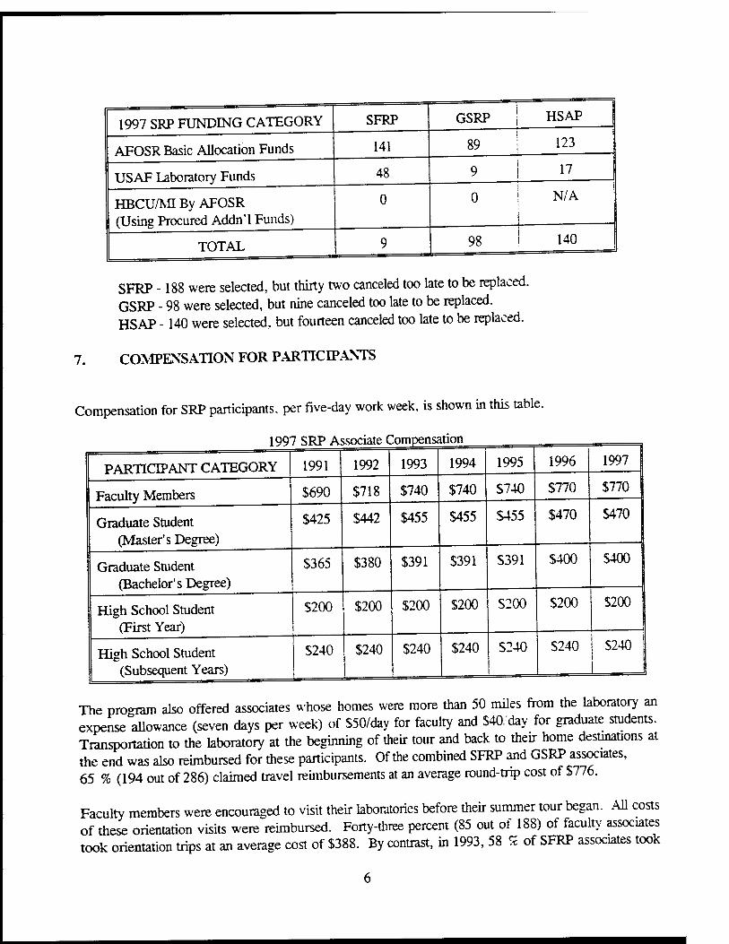
1997 SRP FUNDING CATEGORY SFRP GSRP HSAP j !
AFOSR Basic Allocation Funds 141 89 123 i
USAF Laboratory Funds 48 9 "
HBCU/MI By AFOSR (Using Procured Addn'l Funds)
0 0 N/A
TOTAL 9 98 140
SFRP -188 were selected, but thirty two canceled too late to be replaced. GSRP - 98 were selected, but nine canceled too late to be replaced. HSAP - 140 were selected, but fourteen canceled too late to be replaced.
7. COMPENSATION FOR PARTICIPANTS
Compensation for SRP participants, per five-day work week, is shown in this table.
PARTICIPANT CATEGORY 1991 1992 1993 1994 1995 1996 1997
Faculty Members S690 $718 $740 $740 S740 $770 $770
Graduate Student (Master's Degree)
S425 $442 $455 $455 S455 $470 $470
Graduate Student (Bachelor's Degree)
$365 $380 $391 $391 S391 $400 $400
High School Student (First Year)
$200 $200 $200 $200 S200 $200 $200
High School Student (Subsequent Years)
$240 $240 $240 $240 S240 $240 S240
The program also offered associates whose homes were more than 50 miles from the laboratory an expense allowance (seven days per week) of $50/day for faculty and $40. day for graduate students. Transportation to the laboratory at the beginning of their tour and back to their home destinations at the end was also reimbursed for these participants. Of the combined SFRP and GSRP associates, 65 % (194 out of 286) claimed travel reimbursements at an average round-trip cost of $776.
Faculty members were encouraged to visit their laboratories before their summer tour began. All costs of these orientation visits were reimbursed. Forty-three percent (85 out of 188) of faculty associates took orientation trips at an average cost of $388. By contrast, in 1993, 58 5 of SFRP associates took
orientation visits at an average cost of $685; that was the highest percentage of associates opting to take an orientation trip since RDL has administered the SRP. and the highest average cost of an orientation trip. These 1993 numbers are included to show the fluctuation which can occur in these
numbers for planning purposes.
Program participants submitted biweekly vouchers countersigned by their laboratory research focal point, and RDL issued paychecks so as to arrive in associates' hands two weeks later.
This is the second year of using direct deposit for the SFRP and GSRP associates. The process went much more smoothly with respect to obtaining required information from the associates, only Vx of the associates' information needed clarification in order for direct deposit to properly function as opposed to 10% from last year. The remaining associates received their stipend and expense payments
via checks sent in the US mail.
HSAP proeram participants were considered actual RDL employees, and theix respective state and federal income tax and Social Security were withheld from their paychecks. By the nature of their independent research, SFRP and GSRP program participants were considered to be consultants or independent contractors. As such. SFRP and GSRP associates were responsible for their own income taxes, Social Security, and insurance.
8. CONTENTS OF THE 1997 REPORT
The complete set of reports for the 1997 SRP includes this program management report (Volume 1) augmented by fifteen volumes of final research reports by the 1997 associates, as indicated below:
LABORATORY SFRP GSRP HSAP I
Armstrong 7 12
Phillips 3 8 13
Rome 4 9 ,4 |
Wright 5A, 5B 10 15 ;
AEDC, ALCs, WHMC 6 11 16 :
APPENDIX A - PROGRAM STATISTICAL SUMMARY
A. Colleges/Universities Represented
Selected SFRP associates represented 169 different colleges, universities, and institutions. GSRP associates represented 95 different colleges, universities, and institutions.
B. States Represented
SFRP -Applicants came from 47 states plus Washington D.C. Selectees represent 44 states.
GSRP - Applicants came from 44 states. Selectees represent 32 states.
HSAP - Applicants came from thirteen states. Selectees represent nine states.
j Total Number of Participants
1 SFRP 189
I GSRP 97
HSAP 140
TOTAL 426
1 Degrees Represented
SFRP GSRP TOTAL
Doctoral 184 0 184
Master's 2 41 43
1 Bachelor's 0 56 56 J
1 TOTAL 186 97 298 |
A-l
SFRP Academic Titles
Assistant Professor
Associate Professor
Professor
Instructor
Chairman
Visiting Professor
Visiting Assoc. Prof.
Research Associate
TOTAL
64
70
40
186
Source of Learning About the SRP
Category Applicants Selectees
Applied/participated in prior years 28% 34%
Colleague familiar with SRP 19% 16%
Brochure mailed to institution 23% 17%
Contact with Air Force laboratory 17% 23%
IEEE Spectrum 2% 1%
BUHE 1% 1%
Other source 10% 8%
TOTAL i 100% 100%
A-2
APPENDIX B - SRP EVALUATION RESPONSES
1. OVERVIEW
Evaluations were completed and returned to RDL by four groups at the completion of the SRP. The number of respondents in each group is shown below.
Table B-l. Total SRP Evaluations Received
Evaluation Group Responses
SFRP & GSRPs 275
HSAPs 113
USAF Laboratory Focal Points 84
USAF Laboratory HSAP Mentors 6
All groups indicate unanimous enthusiasm for the SRP experience.
The summarized recommendations for program improvement from both associates and laboratory personnel are listed below:
A. Better preparation on the labs' part prior to associates' arrival (i.e., office space, computer assets, clearly defined scope of work).
B. Faculty Associates suggest higher stipends for SFRP associates.
Both HSAP Air Force laboratory mentors and associates would like the summer tour extended from the current 8 weeks to either 10 or 11 weeks; the groups state it takes 4- 6 weeks just to get high school students up-to-speed on what's going on at laboratory. (Note: this same argument was used to raise the faculty and graduate student participation time a few years ago.)
B-l
2. 1997 USAF LABORATORY FOCAL POINT (LFP) EVALUATION RESPONSES
The summarized results listed below are from the 84 LFP evaluations received.
1. LFP evaluations received and associate preferences:
How Many Associates Would You Prefer To Get 1 (% Response)
Lab Evals Recv'd
0 SFRP
1 2 3+ GSRP (w/Univ Professor) 0 12 3+
GSRP (w/o L'niv Professor) 0 12 3+
AEDC WHMC AL USAFA PL RL WL
0 0 7 1
25 5
46
28 0 40 60 30
28 28 100 0 40 16 40 0 43 20
14 0 4 0 6
54 14 28 0 100 0 0 0 88 12 0 0 80 10 0 0 78 17 4 0
86 0 14 0 100 0 84 12 4 100 0 0 93 4 2
0 0 0 0 0
Total 84 32% 50% 13% 5% 80% 11% 6% 0% 73% 23% 4% 0%
LFP Evaluation Summary. The summarized responses, by laboratory, are listed on the following page. LFPs were asked to rate the following questions on a scale from 1 (below average) to 5 (above
average).
2. LFPs involved in SRP associate application evaluation process: a. Time available for evaluation of applications: b. Adequacy of applications for selection process:
3. Value of orientation trips: 4. Length of research tour: 5 a. Benefits of associate's work to laboratory:
b. Benefits of associate's work to Air Force: 6. a. Enhancement of research qualifications for LFP and staff:
b. Enhancement of research qualifications for SFRP associate: c. Enhancement of research qualifications for GSRP associate: a. Enhancement of knowledge for LFP and staff: b. Enhancement of knowledge for SFRP associate: c. Enhancement of knowledge for GSRP associate:
Value of Air Force and university links: Potential for future collaboration:
a. Your working relationship with SFRP: b. Your working relationship with GSRP:
11. Expenditure of your time worthwhile: (Continued on next page)
7
8. 9. 10.
B-2
12. Quality of program literature for associate: 13. a. Quality of RDL's communications with you:
b. Quality of RDL's communications with associates: 14. Overall assessment of SRP:
Table'. B-3. Laboratory Focal Point Reponses to above questions AEDC AL USAFA PL RL WHMC \\L
# Evals Recv'd 0 1 1 14 5 0 46 Question #
2 - 86 % 0 % 88% 80% - 85 % 2a - 4.3 n/a 3.8 4.0 - 3.6 2b - 4.0 n/a 3.9 4.5 - 4.1 3 - 4.5 n/a 4.3 4.3 - 3.7 4 - 4.1 4.0 4.1 4.2 - 3.9 5a - 4.3 5.0 4.3 4.6 - 4.4 5b - 4.5 n/a 4.2 4.6 - 4.3 6a - 4.5 5.0 4.0 4.4 - 4.3 6b - 4.3 n/a 4.1 5.0 - 4.4 6c - 3.7 5.0 3.5 5.0 - 4.3 7a - 4.7 5.0 4.0 4.4 - 4.3 7b - 4.3 n/a 4.2 5.0 - 4.4 7c - 4.0 5.0 3.9 5.0 - 4.3 8 - 4.6 4.0 4.5 4.6 - 4.3 9 - 4.9 5.0 4.4 4.8 - 4.2
10a - 5.0 n/a 4.6 4.6 - 4.6 10b - 4.7 5.0 3.9 5.0 - 4.4 11 - 4.6 5.0 4.4 4.8 - 4.4 12 - 4.0 4.0 4.0 4.2 - 3.8 13a - 3.2 4.0 3.5 3.8 - 3.4 13b - 3.4 4.0 3.6 4.5 - 3.6 14 - 4.4 5.0 4.4 4.8 - 4.4
B-3

3. 1997 SFRP & GSRP EVALUATION RESPONSES
The summarized results listed below are from the 257 SFRP/GSRP evaluations received.
Associates were asked to rate the following questions on a scale from 1 (below average) to 5 (above al™ by ^ Force0 baSe results and over-all results of the 1997 evaluations are hsted after the
questions.
1. The match between the laboratories research and your field: 2. Your working relationship with your LFP: 3. Enhancement of your academic qualifications: 4. Enhancement of your research qualifications: 5. Lab readiness for you: LFP, task, plan: 6. Lab readiness for you: equipment, supplies, facilities:
7. Lab resources: 8. Lab research and administrative support: 9. Adequacy of brochure and associate handbook: 10. RDL communications with you: 11. Overall payment procedures: 12. Overall assessment of the SRP: 13. a. Would you apply again?
b. Will you continue this or related research? 14 Was length of your tour satisfactory? 15. Percentage of associates who experienced difficulties in finding housing: 16. Where did you stay during your SRP tour?
a. At Home: b. With Friend: c. On Local Economy: d. Base Quarters:
17. Value of orientation visit: a. Essential: b. Convenient: c. Not Worth Cost: d. Not Used:
SFRP and GSRP associate's responses are hsted in tabular format on the following page.
B-4
Table B-4. 1997 SFRP & GSRP Associate Responses to SRP Evaluation
Arnold Brooks Edward» Eftlin Griffii flan-vnm Kelly rurtlaud LmkLuid Robin» Tj-niiü WPAFB average
* rss
6 48 6 14 31 19 3 32 1 2 1(1 85 257
1 4.8 4.4 4.6 4.7 4.4 4.9 4.6 4.6 5.0 5.0 4.0 4.7 4.6 i 5.0 4.6 4.1 4.9 4.7 4.7 5.0 4.7 5.0 5.0 4.6 4.8 4.7 3 4.5 4.4 4.0 4.6 4.3 4.2 4.3 4.4 5.0 5.0 4.5 4.3 4.4 4 4.3 4.5 3.8 4.6 4.4 4.4 4.3 4.6 5.0 4.0 4.4 4.5 4.5 s 4.5 4.3 3.3 4.8 4.4 4.5 4.3 4.2 5.0 5.0 3.9 4.4 4.4 6 4.3 4.3 3.7 4.7 4.4 4.5 4.0 3.8 5.0 5.0 3.8 4.2 4.2 7 4.5 4.4 4.2 4.8 4.5 4.3 4.3 4.1 5.0 5.0 4.3 4.3 4.4 8 4.5 4.6 3.0 4.9 4.4 4J 4.3 4.5 5.0 5.0 4.7 4.5 4.5 9 4.7 4.5 4.7 4.5 4.3 4.5 4.7 4.3 5.0 5.0 4.1 4.5 4.5 10 4.2 4.4 4.7 4.4 4.1 4.1 4.0 4.2 5.0 4.5 3.6 4.4 4.3 U 3.8 4.1 4.5 4.0 3.9 4.1 4.0 4.0 3.0 4.0 3.7 4.0 4.0 U 5.7 4.7 4.3 4.9 4.5 4.9 4.7 4.6 5.0 4.5 4.6 4.5 4.6
Numbers below are percentases 13a 83 90 83 93 87 75 100 81 100 100 100 86 87 13b 100 89 83 100 94 98 100 94 100 100 100 94 93 14 83 96 100 90 87 80 100 92 100 100 70 84 88 15 17 6 0 33 20 76 33 25 0 100 20 8 39
16a . 26 17 9 38 23 33 4 - - - 30 16b 100 33 . 40 - 8 - - - - 36 2 16c . 41 83 40 62 69 67 96 100 100 64 68 16d . . . . . - . - - - - 0 17a . 33 100 17 50 14 67 39 - 50 40 31 35 17b . 21 . 17 10 14 - 24 - 50 20 16 16 17c - . . . 10 7 - . - - - 2 3 17d 100 46 - 66 30 69 33 37 100 - 40 51 46
B-5

4. 1997 USAF LABORATORY HSAP MENTOR EVALUATION RESPONSES
Not enough evaluations received (5 total) from Mentors to do useful summary.
B-6
5. 1997 HSAP EVALUATION RESPONSES
The summarized results Usted below are from the 113 HSAP evaluations received.
HSAP apprentices were asked to rate the following questions on a scale from 1 (below average) to 5 (above average)
1. Your influence on selection of topic/type of work. 2. Working relationship with mentor, other lab scientists. 3. Enhancement of your academic qualifications. 4. Technically challenging work. 5. Lab readiness for you: mentor, task, work plan, equipment. 6. Influence on your career. 7. Increased interest in math/science. 8. Lab research & administrative support. 9. Adequacy of RDL's Apprentice Handbook and administrative materials. 10. Responsiveness of RDL communications. 11. Overall payment procedures. 12. Overall assessment of SRP value to you. 13. Would you apply again next year? Yes (92 %) 14. Will you pursue future studies related to this research? Yes (68 %) 15. Was Tour length satisfactory? Yes (82 %)
Arnold Brooks Edwards Ed in Griffiss Hanscom Kirtland Tvndall WPAFB Totals
resp 5 19 7 15 13 2 7 5 40 113
1 2
2.8 4.4
3.3 4.6
3.4 4.5
3.5 4.8
3.4 4.6
4.0 4.0
3.2 4.4
3.6 4.0
3.6 4.6
3.4 4.6
3 4
4.0 3.6
4.2 3.9
4.1 4.0
4.3 4.5
4.5 4.2
5.0 5.0
4.3 4.6
4.6 3.8
4.4 4.3
4.4 4.2
5 6
4.4 3.2
4.1 3.6
3.7 3.6
4.5 4.1
4.1 3.8
3.0 5.0
3.9 3.3
3.6 3.8
3.9 3.6
4.0 3.7
7 8
2.8 3.8
4.1 4.1
4.0 4.0
3.9 4.3
3.9 4.0
5.0 4.0
3.6 4.3
4.0 3.8
4.0 4.3
3.9 4.2
9 10
4.4 4.0
3.6 3.8
4.1 4.1
4.1 3.7
3.5 4.1
4.0 4.0
3.9 3.9
4.0 2.4
3.7 3.8
3.8 3.8
11 12
4.2 4.0
4.2 4.5
3.7 4.9
3.9 4.6
3.8 4.6
3.0 5.0
3.7 4.6
2.6 4.2
3.7 4.3
3.8 4.5
Numbers below , ire percenta ses
13 14
60% 20%
95% 80%
100% 71%
100% 80%
85% 54%
100% 100%
100% 71%
100% 80%
90% 65%
92% 68%
15 100% 70% 71% 100% 100% 50% 86% 60% 80% 82%
B-7
TEMPORAL AND SPATIAL CHARACTERISATION OF A SYNCHRONOUSLY-PUMPED
PERIODICALLY-POLED LITHIUM NIOBATE OPTICAL PARAMETRIC OSCILLATOR
Dr. Graham R. Allan
Assistant Professor
Department of Physics
New Mexico Highlands University
National Avenue
Las Vegas NM 87701
Final Report for:
Summer Faculty Research Program
Phillips Laboratory
Sponsored By:
Air Force Office of Scientific Research
Boiling Air Force Base
Washington DC
&
Phillips Laboratory
August 97
1-1

TEMPORAL AND SPATIAL CHARACTERISATION OF A SYNCHRONOUSLY-PUMPED PERIODICALLY-POLED LITHIUM NIOBATE OPTICAL PARAMETRIC OSCILLATOR
Graham R. Allan
Abstract
The successful operation and characterisation of a synchronously pumped optical parametric oscillator is reported.
The OPO uses an optically pumped (cw-modelocked Nd:YAG laser) 5 cm crystal of periodically-poled lithium
niobate in a temperature stabalised oven. The OPO produces pulses of -100 ps duration in the wavelength range of
~1.5|im. Anomalous switching behaviour has been observed when the system is near synchronism and a reduction
in the transmitted pump noise is seen for incident powers around threshold. Strong pump depletionwas observed in
both the spatial and temporal profiles of the pump. Parasitic losses in the signal involving mixing and second
harmonic generation were observed.
1-2
TEMPORAL AND SPATIAL CHARACTERISATION OF A SYNCHRONOUSLY-PUMPED
PERIODICALLY-POLED LITHIUM NIOBATE OPTICAL PARAMETRIC OSCILLATOR
Graham R. Allan
Introduction
Optical parametric oscillators, OPO's, are now well established as a means of generating widely-tunable coherent
radiation in regions of the electromagnetic spectrum which are normally difficult to access via conventional coherent
sources. However, "low" output powers still limits the utility of OPO's as a tool in nonlinear optics research. In
addressing this limitation we continue to investigate Periodically-Poled Lithium Niobate, PPLN, in a synchronously
pumped OPO. Previous work reported on the characterisation of a 13 mm crystal of PPLN in a synchronously
pumped OPO; in this report the experimental work concentrates on a higher-gain system. As the small-signal gain
is proportional to the square of the gain medium length, a longer crystal of PPLN is used. The dynamics of this
synchronously pumped OPO are again characterised using standard cw and temporally and spatially resolved detection
techniques. This allows study of dynamical effects within an individual pulse, such as pump depletion and back
conversion.
Experimental
The experimental system consists of essentially three components; the pump laser, the OPO and the diagnostics. A
schematic of the general experimental layout is shown in figure 1. The pump source is a commercial, cw, mode-
locked ND:YAG laser operating at 1.064 p.m and producing nominally 100 ps FWHM pulses in a 76 MHz train
with ~20 W of average power. Before injection into the OPO cavity the pump laser is mechanically chopped at
40 Hz with a 100:1 duty cycle. The peak intensity is controlled by the halfwave plate and analyzer (HWPP) and
monitored by a photodetector. In our experiments the mechanical chopping reduces the average power of the pump
laser seeding the OPO to -100 mW. The crystal is maintained at a temperature 60° C which has the effect of
postponing the onset of photorefraction in lithium niobate, in our case almost indefinitely. The nonlinear optical
crystal, a piece of periodically poled lithium niobate, is 50 mm x 10 mm by 500 (im thick with several poled
regions aligned along the long axis. The input and output surfaces of the chip are anti-reflection coated with a
1-3
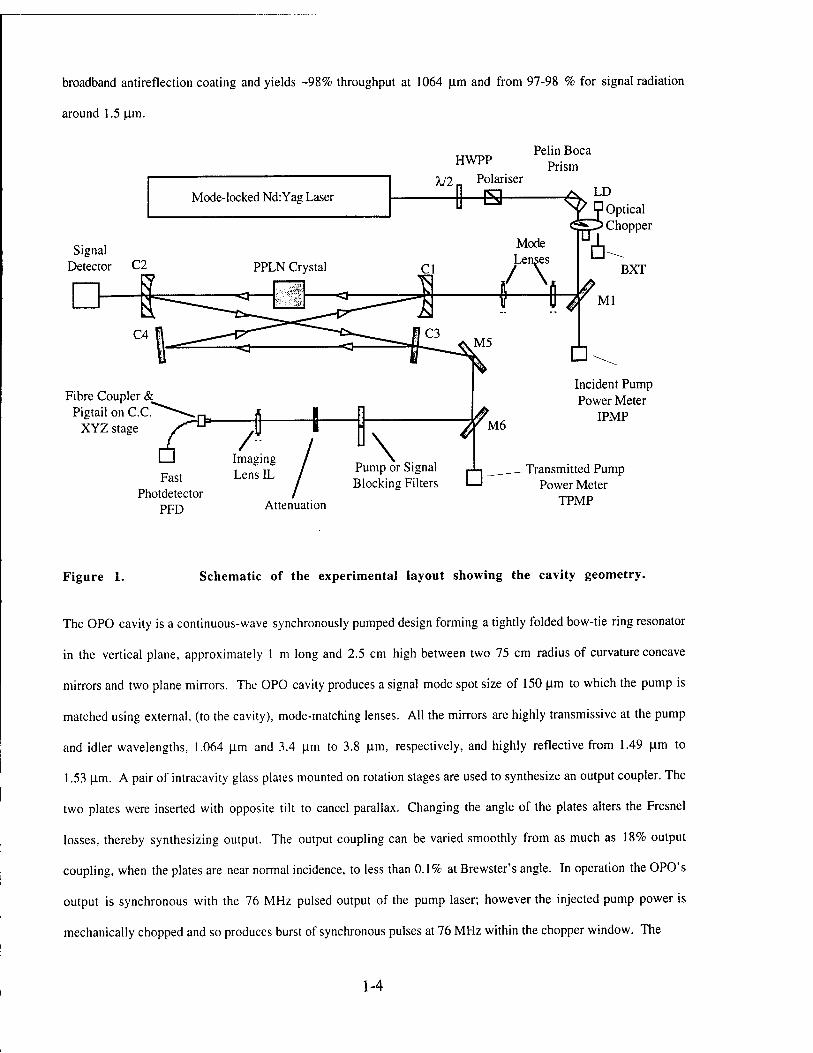
broadband antireflection coating and yields -98% throughput at 1064 |im and from 97-98 % for signal radiation
around 1.5 io.m.
Pelin Boca HWPP Prism
X/2 Polariser
" -H Mode-locked Nd:Yag Laser
Signal Detector C2
Fibre Coupler &_ Pigtail on CC."
XYZ stage r Fast
Photdetector PFD
Imaging Lens IL
D\ Pump or Signal Blocking Filters
K M6
D Attenuation
Incident Pump Power Meter
IPMP
Transmitted Pump Power Meter
TPMP
Figure 1. Schematic of the experimental layout showing the cavity geometry.
The OPO cavity is a continuous-wave synchronously pumped design forming a tightly folded bow-tie ring resonator
in the vertical plane, approximately 1 m long and 2.5 cm high between two 75 cm radius of curvature concave
mirrors and two plane mirrors. The OPO cavity produces a signal mode spot size of 150 ^m to which the pump is
matched using external, (to the cavity), mode-matching lenses. All the mirrors are highly transmissive at the pump
and idler wavelengths, 1.064 urn and 3.4 |im to 3.8 |im, respectively, and highly reflective from 1.49 |im to
1.53 |im. A pair of intracavity glass plates mounted on rotation stages are used to synthesize an output coupler. The
two plates were inserted with opposite tilt to cancel parallax. Changing the angle of the plates alters the Fresnel
losses, thereby synthesizing output. The output coupling can be varied smoothly from as much as 18% output
coupling, when the plates are near normal incidence, to less than 0.1% at Brewster's angle. In operation the OPO's
output is synchronous with the 76 MHz pulsed output of the pump laser; however the injected pump power is
mechanically chopped and so produces burst of synchronous pulses at 76 MHz within the chopper window. The
1-4
chopper blade clears the incident pump beam in ~25|is and the chopper window remains open for approximately 250
(is. The OPO typically reaches steady state in less than 50 (is, after which the output power remains constant until
the chopper window closes. The long term stability of the system was good - typical characterisation runs can take
approximately an hour, over which time the OPO was well behaved and continued to display such behavior over
many hours.
The rest of the system comprises the diagnostics, which are designed to simultaneously monitor the averaged
incident pump power, transmitted pump power and signal power, and the temporally and spatially resolved
transmitted pump or signal. To monitor the averaged powers we used slow-response, large-area, photodetectors to
integrate over the spatial and temporal profiles of the mode-locked pulses from the laser and OPO: The incident
pump power is monitored with photodetector (IPMP); the signal power transmitted through high-reflectivity mirror
(C2) is monitored by photodetector (SIG) and the residual pump power transmitted through the lithium niobate
crystal (PPLN); and cavity high-reflector (C3) is picked off by a beam splitter (BS) and monitored by photodetector
(TPMP). For spatial and temporal resolution we use a fast-response, small-area, fiber-coupled photodetector and a
series of dichroic filters. The input end of the fiber is positioned in the image plane of an optical system that images
the output face of the PPLN OPO crystal. The 75 cm curved mirror on the left of the diagram and a lens (IL) act as
a compound optical system that images the output of the PPLN crystal into a plane where the input end of the
optical fiber is scanned. The position of the image plane is determined by inserting a mask in the OPO cavity at
the output face of PPLN crystal. This partially blocks a weak incident pump and produces a well known interference
pattern. Spatial scans were then performed to exactly determine the image plane. Transverse translation of the mask
by a known amount and recording the spatial profile allowed us to deduce the magnification of the imaging system.
The output end of the optical fiber is connected to a fast-response photodiode (FPD). The dichroic filters (DF) are
mounted on a motorized translation stage to allow computer controlled monitoring of signal or pump wavelengths.
A boxcar integrator, triggered by an auxiliary laser diode (LD) and photodiode (BXT) is used to measure the slow
large-area photodetector voltages. The integrating window is 30(is long and is positioned approximately 175(is from
the opening edge of the chopper window. This is well within the steady state operation of the system. The signal
from the fast-response photodiode is sent to an analog sampling head. The sampling head is triggered by the 38
MHz signal that drives the pump-laser's mode locker. The delay between the triggering and sampling of the
1-5
photodiode's electrical signal is controlled by the computer through an external input of the sampling head. The
temporal resolution of the sampling head binning enabled us to resolve structure of the order of 20 ps The output of
the sampling head was sent to the boxcar triggered at the chopper frequency. The boxcar's integrating window's
width and delay ware adjusted within the chopper window enabling one to temporally resolve the transmitted pump
and signal behaviour through switch-on to steady state. The output voltages of the integrator were recorded by
computer.
Results and Discussions
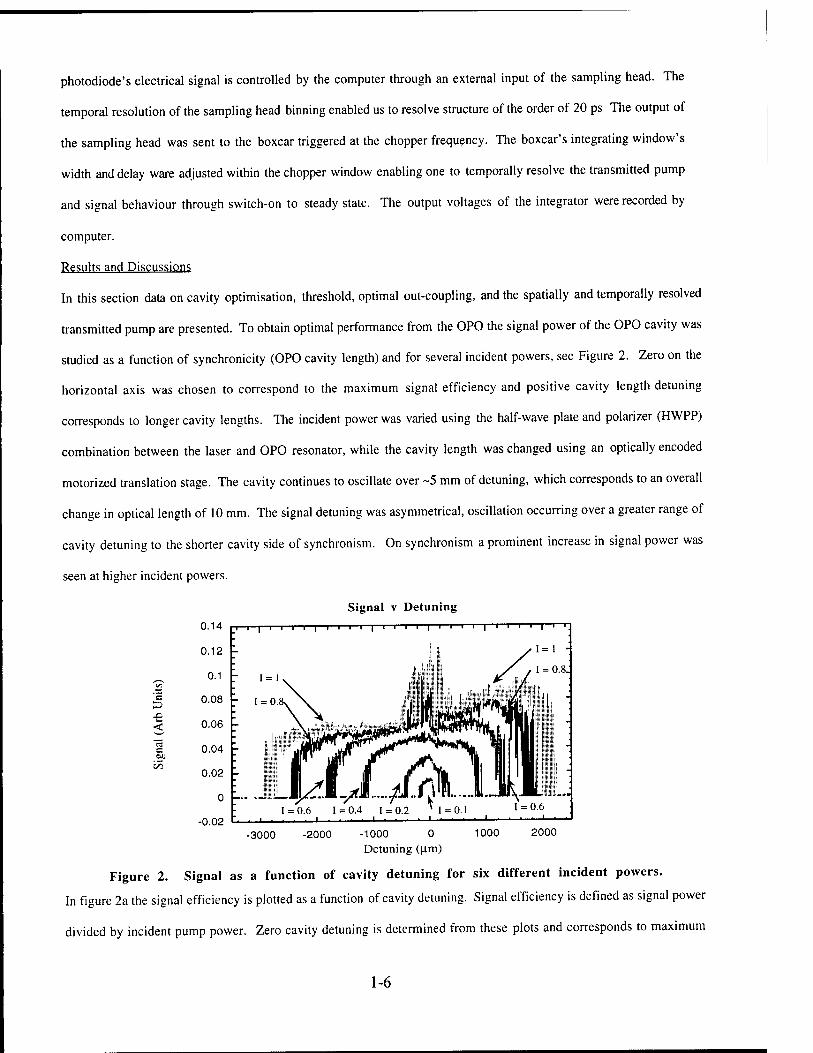
In this section data on cavity optimisation, threshold, optimal out-coupling, and the spatially and temporally resolved
transmitted pump are presented. To obtain optimal performance from the OPO the signal power of the OPO cavity was
studied as a function of synchronicity (OPO cavity length) and for several incident powers, see Figure 2. Zero on the
horizontal axis was chosen to correspond to the maximum signal efficiency and positive cavity length detuning
corresponds to longer cavity lengths. The incident power was varied using the half-wave plate and polarizer (HWPP)
combination between the laser and OPO resonator, while the cavity length was changed using an optically encoded
motorized translation stage. The cavity continues to oscillate over ~5 mm of detuning, which corresponds to an overall
change in optical length of 10 mm. The signal detuning was asymmetrical, oscillation occurring over a greater range of
cavity detuning to the shorter cavity side of synchronism. On synchronism a prominent increase in signal power was
seen at higher incident powers.
Signal v Detuning
x; <
cJ5
-3000 -2000 -1000 0 Detuning (um)
1000 2000
Figure 2. Signal as a function of cavity detuning for six different incident powers.
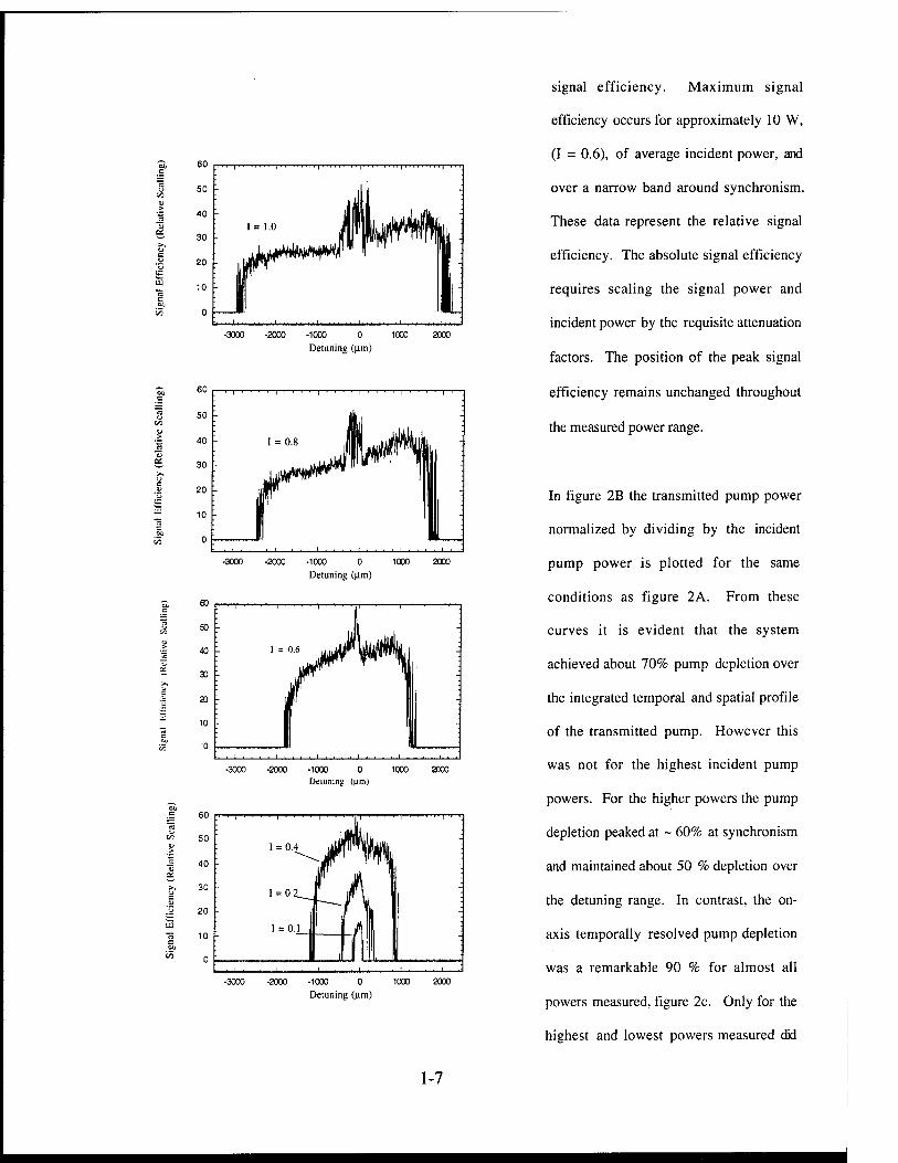
In figure 2a the signal efficiency is plotted as a function of cavity detuning. Signal efficiency is defined as signal power
divided by incident pump power. Zero cavity detuning is determined from these plots and corresponds to maximum
1-6
•3000 -2000 -1000 0 1000 Detuning (um)
-3000 -2000 -1000
Detuning 0
(Um) 1000 2000
-3000 -2000 -1000
Detuning 0
(um) 1000 2000
signal efficiency. Maximum signal
efficiency occurs for approximately 10 W,
(I = 0.6), of average incident power, and
over a narrow band around synchronism.
These data represent the relative signal
efficiency. The absolute signal efficiency
requires scaling the signal power and
incident power by the requisite attenuation
factors. The position of the peak signal
efficiency remains unchanged throughout
the measured power range.
In figure 2B the transmitted pump power
normalized by dividing by the incident
pump power is plotted for the same
conditions as figure 2A. From these
curves it is evident that the system
achieved about 70% pump depletion over
the integrated temporal and spatial profile
of the transmitted pump. However this
was not for the highest incident pump
powers. For the higher powers the pump
depletion peaked at ~ 60% at synchronism
and maintained about 50 % depletion over
the detuning range. In contrast, the on-
axis temporally resolved pump depletion
was a remarkable 90 % for almost all
powers measured, figure 2c. Only for the
highest and lowest powers measured did
1-7
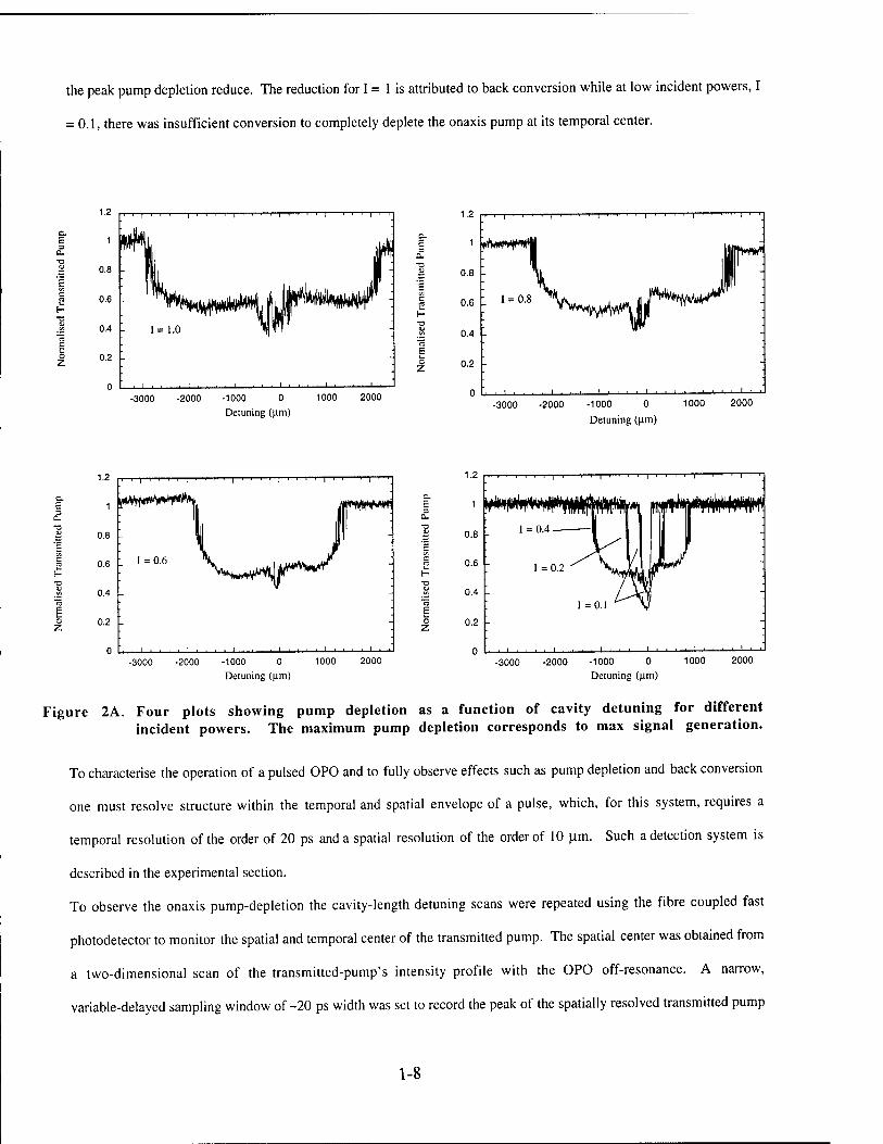
the peak pump depletion reduce. The reduction for I = 1 is attributed to back conversion while at low incident powers, I
= 0.1, there was insufficient conversion to completely deplete the onaxis pump at its temporal center.
-3000 -2000 -1000 0 Detuning (urn)
1000 2000
E Q.
-3000 -2000 -1000 0 Detuning (|im)
1000 2000
E a.
E e
-3000 -2000 -1000 0 Detuning (urn)
t»W+m
1000 2000
E o Z
-3000 -2000 -1000 0 Detuning (um)
1000 2000
Figure 2A. Four plots showing pump depletion as a function of cavity detuning for different incident powers. The maximum pump depletion corresponds to max signal generation.
To characterise the operation of a pulsed OPO and to fully observe effects such as pump depletion and back conversion
one must resolve structure within the temporal and spatial envelope of a pulse, which, for this system, requires a
temporal resolution of the order of 20 ps and a spatial resolution of the order of 10 (im. Such a detection system is
described in the experimental section.
To observe the onaxis pump-depletion the cavity-length detuning scans were repeated using the fibre coupled fast
photodetector to monitor the spatial and temporal center of the transmitted pump. The spatial center was obtained from
a two-dimensional scan of the transmitted-pump's intensity profile with the OPO off-resonance. A narrow,
variable-delayed sampling window of -20 ps width was set to record the peak of the spatially resolved transmitted pump
1-8
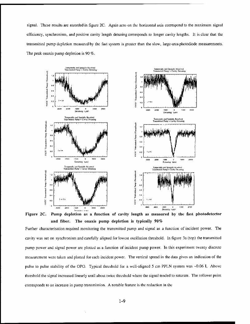
signal. These results are recorded in figure 2C. Again zero on the horizontal axis correspond to the maximum signal
efficiency, synchronism, and positive cavity length detuning corresponds to longer cavity lengths. It is clear that the
transmitted pump depletion measured by the fast system is greater than the slow, large-area photodiode measurements.
The peak onaxis pump depletion is 90 %.
Temporally and Spatially Resolved Transmitted Pump v Cavity Detuning ,-
1.2
Temporally and Spatially Resolved Transmitted Pump v Cavity Detuning
£ c Z c
o.e ' VB ii lm '• ■p
0.6 ifl "ll| Jflf §
0.4 £
*v 0.2 i = i.o 'flftyHiU Jnilri^r < "™
-3000 -2000 -1000 0 1000 2000
Detuning (Jim)
Temporally and Spatially Resolved Transmitted Pump v Cavity Detuning
-3000 -2000 -1000 0 1000 2000 Detuning (Jim)
Temporally and Spatially Resolved Transmitted Pump v Cavity Detuning
-3000 -2000 -1000 0 1000 2000
Detuning <|im) •3000 -2000 -1000 0 1000 2000
Detuning (pm)
_ 1.2
Temporally Transmitted
and Spatially Resolved Pump v Cavity Detuning
~ i'' i' i ' 'llilliil i i :
s c 7 , IIAfi c-
o.e flrli,™|rnji7 f
■In "3 0.6 if E UL
5 0.4 Jfl
< 0.2 ■_ I = 0.6 Mm
Temporally and Spatially Resolved Transmitted Pump v Cavity Detuning
1.2 1 z
III III Ml I »if c. 0.8 Wlffl' 1 ff V ff :
1 0.6 I 1 0.4
M ^ 0.2 _ 1=0.1 [1 <
i c ...........-
•3000 -2000 -1000 1000 2000 ■3000 -2000 -1000 0 1000 2000
Detuning Him)
Figure 2C. Pump depletion as a function of cavity length as measured by the fast photodetector
and fiber. The onaxis pump depletion is typically 90%
Further characterisation required monitoring the transmitted pump and signal as a function of incident power. The
cavity was set on synchronism and carefully aligned for lowest oscillation threshold. In figure 3a (top) the transmitted
pump power and signal power are plotted as a function of incident pump power. In this experiment twenty discrete
measurement were taken and plotted for each incident power. The vertical spread in the data gives an indication of the
pulse to pulse stability of the OPO. Typical threshold for a well-aligned 5 cm PPLN system was -0.06 I, Above
threshold the signal increased linearly until about twice threshold where the signal tended to saturate. The rollover point
corresponds to an increase in pump transmission. A notable feature is the reduction in the
1-9
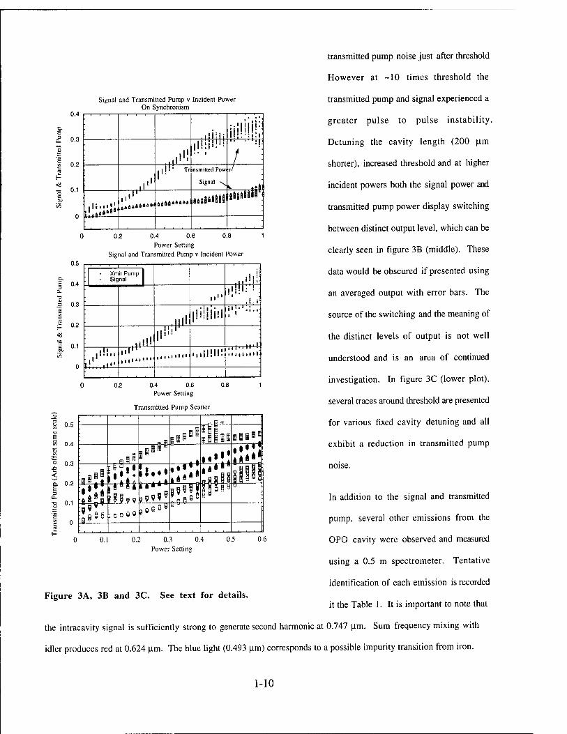
0.4
a.
£, 0.3
1 °-2
«a - 0.1 c to
Signal and Transmitted Pump v Incident Power On Synchronism
i ..aÄ.""_
rf¥
im mtm Transmitted Pow^r
Signal
iipl!;:
*!
0.2 0.8 0.4 0.6 Power Setting
Signal and Transmitted Pump v Incident Power 0.5
E 0.4
= 0.3 E
0.1
Xmit Pump Signal
.I'-1 il.H"
n4^
,,•■■1
|!:!i;i!i
,.i!!M!
nmn
■ ii"i»' .I.,I,III
0.2 0.4 0.6 Power Setting
Transmitted Pump Scatter
0.8
ö 0.5
E S 0.4
° 0.3
< a, 0.2
a. •o 0.1
ll
r4
:?
ft*
rr
o ee
ftr* ?99g3 30 rp" •y_
iii_ iWt
|||SS
•ifii
0.1 0.2 0.3 0.4 Power Setting
0.5 0.6
Figure 3A, 3B and 3C. See text for details.
transmitted pump noise just after threshold
However at -10 times threshold the
transmitted pump and signal experienced a
greater pulse to pulse instability.
Detuning the cavity length (200 |im
shorter), increased threshold and at higher
incident powers both the signal power and
transmitted pump power display switching
between distinct output level, which can be
clearly seen in figure 3B (middle). These
data would be obscured if presented using
an averaged output with error bars. The
source of the switching and the meaning of
the distinct levels of output is not well
understood and is an area of continued
investigation. In figure 3C (lower plot),
several traces around threshold are presented
for various fixed cavity detuning and all
exhibit a reduction in transmitted pump
noise.
In addition to the signal and transmitted
pump, several other emissions from the
OPO cavity were observed and measured
using a 0.5 m spectrometer. Tentative
identification of each emission is recorded
it the Table 1. It is important to note that
the intracavity signal is sufficiently strong to generate second harmonic at 0.747 urn Sum frequency mixing with
idler produces red at 0.624 urn. The blue light (0.493 |im) corresponds to a possible impurity transition from iron.
1-10
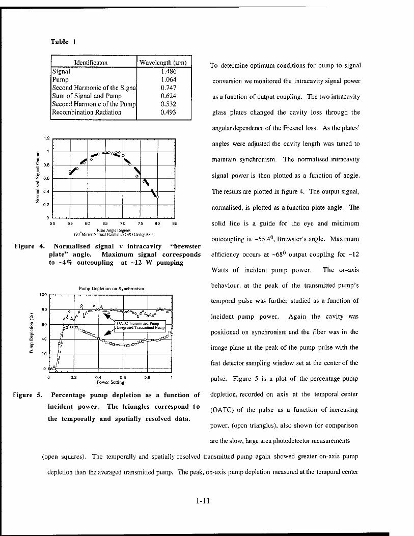
Identificaton Wavelength (um) Signal 1.486 Pump 1.064 Second Harmonic of the Signa 0.747 Sum of Signal and Pump 0.624 Second Harmonic of the Pump 0.532 Recombination Radiation 0.493
Table 1
To determine optimum conditions for pump to signal
conversion we monitored the intracavity signal power
as a function of output coupling. The two intracavity
glass plates changed the cavity loss through the
angular dependence of the Fresnel loss. As the plates'
angles were adjusted the cavity length was tuned to
maintain synchronism. The normalised intracavity
signal power is then plotted as a function of angle.
The results are plotted in figure 4. The output signal,
normalised, is plotted as a function plate angle. The
solid line is a guide for the eye and minimum
outcoupling is -55.4°, Brewster's angle. Maximum Figure 4. Normalised signal v intracavity "brewster
plate" angle. Maximum signal corresponds efficiency occurs at ~68° output coupling for -12 to ~4% outcoupling at -12 W pumping
Watts of incident pump power. The on-axis
behaviour, at the peak of the transmitted pump's
temporal pulse was further studied as a function of
incident pump power. Again the cavity was
positioned on synchronism and the fiber was in the
image plane at the peak of the pump pulse with the
fast detector sampling window set at the center of the
pulse. Figure 5 is a plot of the percentage pump
1.2
1 3 Q.
° 0.8 c CO
'& 0.6 u
1 0.4 o 2 0.2
0
■ ■
* 0
*?<yj£'<
< r \ . ' ^
V >
. 50 55 60 65 70 75 80
0 Plate Angle Degrees (9(1 Mirror Normal Parallel to OPO Cavily Axis)
Pump Depletion on Synchronism
ä 40
0.4 0.6 Power Setting
Figure 5. Percentage pump depletion as a function of depletion, recorded on axis at the temporal center
incident power. The triangles correspond to (0ATQ of the pu,se as fl function of increasing
the temporally and spatially resolved data. power, (open triangles), also shown for comparison
are the slow, large area photodetector measurements
(open squares). The temporally and spatially resolved transmitted pump again showed greater on-axis pump
depletion than the averaged transmitted pump. The peak, on-axis pump depletion measured at the temporal center
1-11
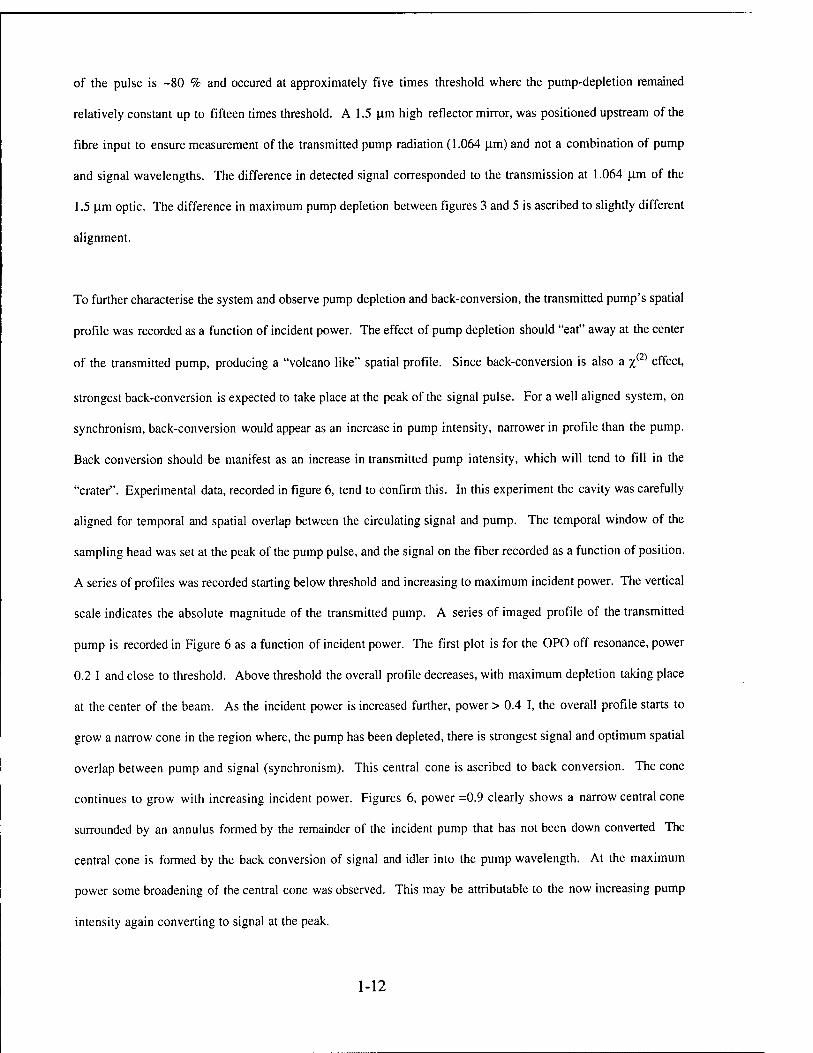
of the pulse is -80 % and occured at approximately five times threshold where the pump-depletion remained
relatively constant up to fifteen times threshold. A 1.5 |im high reflector mirror, was positioned upstream of the
fibre input to ensure measurement of the transmitted pump radiation (1.064 (im) and not a combination of pump
and signal wavelengths. The difference in detected signal corresponded to the transmission at 1.064 |im of the
1.5 (im optic. The difference in maximum pump depletion between figures 3 and 5 is ascribed to slightly different
alignment.
To further characterise the system and observe pump depletion and back-conversion, the transmitted pump's spatial
profile was recorded as a function of incident power. The effect of pump depletion should "eat" away at the center
of the transmitted pump, producing a "volcano like" spatial profile. Since back-conversion is also a x(2) effect,
strongest back-conversion is expected to take place at the peak of the signal pulse. For a well aligned system, on
synchronism, back-conversion would appear as an increase in pump intensity, narrower in profile than the pump.
Back conversion should be manifest as an increase in transmitted pump intensity, which will tend to fill in the
"crater". Experimental data, recorded in figure 6, tend to confirm this. In this experiment the cavity was carefully
aligned for temporal and spatial overlap between the circulating signal and pump. The temporal window of the
sampling head was set at the peak of the pump pulse, and the signal on the fiber recorded as a function of position.
A series of profiles was recorded starting below threshold and increasing to maximum incident power. The vertical
scale indicates the absolute magnitude of the transmitted pump. A series of imaged profile of the transmitted
pump is recorded in Figure 6 as a function of incident power. The first plot is for the OPO off resonance, power
0.2 I and close to threshold. Above threshold the overall profile decreases, with maximum depletion taking place
at the center of the beam. As the incident power is increased further, power > 0.4 I, the overall profile starts to
grow a narrow cone in the region where, the pump has been depleted, there is strongest signal and optimum spatial
overlap between pump and signal (synchronism). This central cone is ascribed to back conversion. The cone
continues to grow with increasing incident power. Figures 6, power =0.9 clearly shows a narrow central cone
surrounded by an annulus formed by the remainder of the incident pump that has not been down converted The
central cone is formed by the back conversion of signal and idler into the pump wavelength. At the maximum
power some broadening of the central cone was observed. This may be attributable to the now increasing pump
intensity again converting to signal at the peak.
1-12
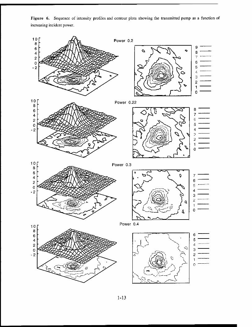
Figure 6. Sequence of intensity profiles and contour plots showing the transmitted pump as a function of
increasing incident power.
Power 0.2
Power 0.22
Power 0.3
Power 0.4
«-I""
* [ \ V X
/"""S ^ f"^- J v XJ.
J-%
(f Sft t ^ SI,
-H, ,A, l^jf' Ll ■"«—if"'"'* jOU-J
""v* ~ 1_nT1_ JH^ jd-^^^-n^^jA
6 5 4 3 2 1 0
1-13
Power 0.5
"^7 \
7 6 5 4 3 2 1 0
Power 0.6
i, K TV
V V, r""
5 4 3 2 1 0
Power 0.7
5 4 3 2 1 0
r t-
Power 0.8
6 5 4 3 2 1 0
1-14
Power 0.9
Power 1.0
»—^s. <T^\ i ff V,-,,X f ^ \ _J
±3^ .--fX
7 6 5 4 3 2 1 0
Temporal Profile
The operation of the OPO from switch-on through steady-state operation was also studied. A considerable wealth
and volume of data was taken during these experiments and only preliminary (raw) data presented here. The onaxis
temporal profiles of the transmitted pump pulse and signal pulse were recorded for various time delays within the
chopper window. Again the fiber was positioned in the image plane at the spatial center of the transmitted pulse.
Due to dispersion and cavity alignment the center of the transmitted pump did not always coincide exactly with the
signal profile. On switching from transmitted pump to signal detection not only was the blocking filter changed
but the fiber was also repositioned for the corresponding center.The following results show typical operation of
OPO for strong pumping and for pump pulse of -100 ps FWHM at various times within the 250 |is chopper
window. The width of each plot is 500 ps. Figure 7 is a composite plot of 6 temporal profiles each taken -30 |is
later than the previous pulse during the chopper window. The first 50 |J.s corresponds to switch-on; after -100 (Xs
the system approaches equilibrium. In the first plot (top) the leading edge of the transmitted pump has already
been depleted in the high gain system at the strongest pumping levels. After -100 |is a strong peak is observed in
the trailing edge of the pulse. This is attributed to back conversion and the system oscillation with a slight cavity
detuning. Switch-off is essentially the reverse of Figure 7.
1-15
Figure 7. Temporal profile of the transmitted pump for different times within the chopper window. The horizontal width is 500 ps.
:
:
: ^S*> **H.i f
2 B ■ta 33 o 8
;
.A :
■ X Vy rV.
2 Data 37
«r w. A / V
**/ i/
%-....,>-< /v"
^tf ; I \
Data 61
A, / * V ̂
»V
Conclusions
In this report the successful operation and
characterisation of 5 cm of PPLN in a cw-modelocked
Nd:YAG synchronously-pumped OPO cavity is
described. The OPO produced pulses of -100 ps duration
in the wavelength range of ~1.5um. Anomalous
switching behaviour was observed when the system was
near synchronism and a reduction in the transmitted
pump noise was seen for incident powers around
threshold. Strong pump depletion was observed in both
the spatial and temporal profiles of the pump.
Acknowledgements. I would like to thank Dr. Karl Koch, Captain Mike Dearborn and Dr Gerald Moore of Phillips Laboratory for their cooperation and assistance throughout all phases of this work. I would also like to acknowledge Phillips Lab, RDL and AFOSR for their support.
1-16
NONLINEAR TRACKING CONTROL FOR A PRECISION DEPLOYABLE STRUCTURE USING A PARTITIONED FILTER APPROACH
Mark J. Balas Professor
Department of Aerospace Engineering Sciences
University of Colorado Boulder, CO 80309-0429
Final Report for: Summer Faculty Research Program
USAF Phillips Laboratory Albuquerque, NM
Sponsored by: Air Force Office of Scientific Research
Boiling Air Force Base, DC
September 1997
2-1
NONLINEAR TRACKING CONTROL FOR A PRECISION DEPLOY ABLE STRUCTURE USING A PARTITIONED FILTER APPROACH
Mark J. Balas Professor
Department of Aerospace Engineering Sciences University of Colorado
Abstract
As part of the Integrated Ground Demonstration Laboratory (IGDL) mission, the
feasibility of a large, deployable, sparse aperture, space telescope is being studied under the
UltraLITE project. Precision tracking of the deployable structure via a speaker voice-coil
actuated white-light interferometer is the subject of this report.
We have established a new tracking control approach using a partitioned Kaiman filter
based on measurements of the actuator current and the normalized fringe intensity from an
avalanche photo diode. This control has the potential to maintain the optical path difference of
the interferometer within desired nanometer tolerances. The theory to support this tracking
controller is developed in this report.
2-2
NONLINEAR TRACKING CONTROL FOR A PRECISION DEPLOYABLE STRUCTURE USING A PARTITIONED FILTER APPROACH
Mark J. Balas
1.0 Introduction
Under the UltraLITE project, experiments are being developed at the US Air Force Phillips
Laboratory to determine the feasibility of large, deployable, sparse aperture, space-based
telescopes. This has resulted in a proposed UltraLITE deployable test structure as part of the
Integrated Ground Demonstration Laboratory (IGDL) to measure and control subwavelength
(nanometer) structural disturbances.
White light interferometry has been chosen to measure accurately structural disturbances on the
nanometer scale. Since the coherence length of white light is on the order of hundreds of
nanometers, the precision structure may induce disturbances well beyond the range of the
interferometer sensor. Consequently, the interferometer must track the structure to produce zero
optical path difference (OPD) to provide structure position without signal loss. This is done
using a voice-coil actuated mirror (called "the Speaker") as the reference optical path. The
speaker must be controlled to lock on and track the structure motion, and that control system is
the subject of this paper.
2.0 The Speaker Model
The voice-coil actuated mirror actually consists of four speaker actuators attached to the mirror
to control piston, tip, and tilt. We focus here on the piston control only and consider a single
speaker:
mx + dx + kx = ß/i (la)
L—+ Ri = V-ß/x (lb) dt
where x is the speaker position, i the speaker current, and V the voltage applied to the speaker.
2-3
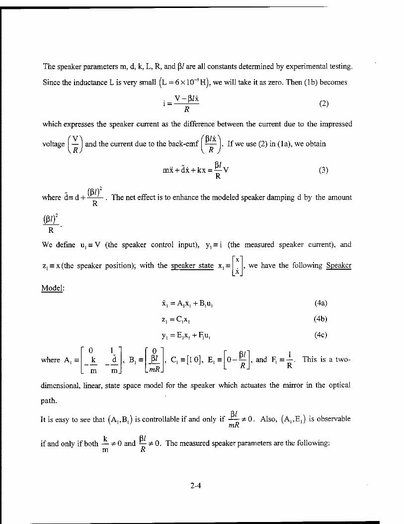
The speaker parameters m, d, k, L, R, and ß/ are all constants determined by experimental testing.
Since the inductance L is very small (L = 6 x IC)-5!!), we will take it as zero. Then (lb) becomes
V-ß/x l = ■
R (2)
which expresses the speaker current as the difference between the current due to the impressed
voltage I — \R)
and the current due to the back-emf V R j
ß' mx + dx + kx = — V R
. If we use (2) in (la), we obtain
(3)
(ßO where d= d + -—— . The net effect is to enhance the modeled speaker damping d by the amount R
M. R
We define u, = V (the speaker control input), y, = i (the measured speaker current), and
we have the following Speaker z, = x (the speaker position); with the speaker state x, = X
X i
Model:
x, = A,x, +B,u,
Z| = L-jX,
y^EiX.+F.u,
where A, = " 0 1
k d . m m.
. B,= " 0 "
ß' .mR.
, C,s[lO], E,s 0 _ß I
(4a)
(4b)
(4c)
1 and F, =—. This is a two- 1 R
dimensional, linear, state space model for the speaker which actuates the mirror in the optical
path.
It is easy to see that (A,,B,) is controllable if and only if —*0. Also, (A,,E,) is observable mR
k ß/ if and only if both — ^0 and — ^ 0. The measured speaker parameters are the following:
m R
2-4
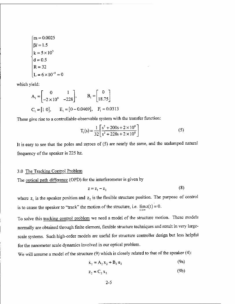
m = 0.0025
ß/ = 1.5
k = 5xl03
d = 0.5
R = 32
L = 6 x 10"5 » 0
which yield:
i \ = " 0 1
-2 x 10⁶ -228 B,=
" 0
18.75
C,=[10], E, =[0-0.0469], F, =0.0313
These give rise to a controllable-observable system with the transfer function:
T,(s) = 32
s2+200s + 2xl06
(5) /+228s + 2xl06
It is easy to see that the poles and zeroes of (5) are nearly the same, and the undamped natural
frequency of the speaker is 225 hz.
3.0 The Tracking Control Problem
The optical path difference (OPD) for the interferometer is given by
£j — £j, £jn (8)
where z, is the speaker position and z2 is the flexible structure position. The purpose of control
is to cause the speaker to "track" the motion of the structure, i.e. limz(t) = 0.
To solve this tracking control problem we need a model of the structure motion. These models
normally are obtained through finite element, flexible structure techniques and result in very large-
scale systems. Such high-order models are useful for structure controller design but less helpful
for the nanometer scale dynamics involved in our optical problem.
We will assume a model of the structure (9) which is closely related to that of the speaker (4):
x2 = A2 x2 + B2 u2 (9a)
z2 = C2 x2 (9b)
2-5
where dimx2 =dimx, =2. This may seem rather arbitrary, but for our needs the structure
model (9) is more of a mental construct or "metamodel" than an actual representation of all the
complex motions of which the structure is capable. As we shall see, only a measurement
involving the OPD is available to our controller, nothing more.
Define the state error
e = x,-x2 (10)
and obtain, from (4) and (9), the following:
e = A^ + E^u, +(A, -A2)X2 -B2u2 (11)
The form of an ideal tracking control law would be
U;=G,e + Gxx2+Guu2 (12)
This results in a closed-loop system:
e = (A1 + B,G1)e + [A] + B1Gx-A2]x2+[N1Gu-B2]u2 (13)
and the following OPD:
z = z, -z2 =C,x, -C2x2 =C,e + [C, -C2]x2 (14)
If a set of matching conditions:
A2=A,+B1GX (15a)
B2=B,GU (15b)
C,=C2 (15c)
can be satisfied, the closed-loop (13) becomes
Je = (A,+B1G1)e (16a)
[z = C,e (16b)
Then the controllability of (A,,B,) permits the choice of control gains Gi to achieve arbitrary
exponential convergence (lim e = 0) and, hence, z = Ce -» 0. The rate of convergence will be
determined by the eigenvalues of A, H-B^,. The matching conditions (15) simply say that it is
possible, via feedback, to match the structure and speaker motions. If they could not be
satisfied, the speaker would not be capable of tracking the structure motion, i.e. limz * 0.
2-6
There are limitations to the ideal control law (12):
(a) e and x2 are not measured
(b) u2 is not measured
For our development (b) is not critical since we may assume u2 = 0 in (9); this means our
metamodel is not "driven" by any (deterministic) exogenous inputs. However, (a) must be
addressed.
In the next sections, we will develop estimators for X] and x2 from available
measurements. This will allow us to create a realizable tracking control law.
4.0 The Linear Speaker Filter
Since (Ai, E^ is observable, it is possible to recover the speaker position z( (and velocity, too)
from the measured current via a linear state estimator or Kaiman filter:
fx, = A,x, +B,u, +K,(y, -y,) (17a)
[y1=EIx1+FIu1 (17b)
The input and output noise covariances can be estimated for the speaker and used to solve for the
filter gains K( using the Riccati equation, e.g. [2]. Alternatively, a deterministic approach using
the speaker estimator error e, = x, - x, yields:
e.^A.-K.Eje, (18)
where the filter gains K( can be chosen by arbitrary pole placement since (Ai, E{) is observable.
In either case, the estimated speaker state x, will converge exponentially fast to the actual state
X! with rate determined by the eigenvalues of A, - K,E,.
5.0 The Nonlinear Structure Filter
There is no way to measure the OPD directly. Instead it is indirectly measured from the
interferometer using an avalanche photo diode (APD) whose output is the normalized intensity:
y2 = h(z) (19)
where the nonlinear fringe function h(-) is given by
2-7
h(z) = —+ —e w 2 2
lf4^U f*^ COS
47CZ (20)
with center wave length Xc ~ 600 nm and passband ?ip ~ lOOnm for our testbed. This function
can be derived for a white light interferometer in Twyman-Green configuration; see developments
in [3] Chapter 22 and [4] Chapter VII.
A nonlinear state estimator, or extended Kaiman filter, can be used to recover the structure state
x2 from the APD output y2; for details, see [5] Chapter 6 or [6] Chapter 6. Our nonlinear
structure filter is given by
x2=A2x2 + K2(y2-y2) (21a)
y2=h(z) (21b)
(21c)
where z is the estimated OPD and z, and z2 are the estimated speaker and structure position
estimates, respectively.
The linearized structure filter is given by
x2=A2x2 + K2(y2-y2)
y2=Hz
~~ 1 1
(22a)
(22b)
(22c)
where (22b) replaces (21b) and
H _ dh(«
<£ 1 - ' r 1 = --e"aZo,,[2azopcosbzop +bsinbzopJ (23)
5=z„
and a = — 4
4rc-^ 4TTZ
and b = . We see that h(-) is locally invertible when H*0; we will
pick any zop where H ^ 0.
Define the structure state estimation error e2 = x2 - x2. From (9) and (22) with (19) linearized
by y2 = Hz, we obtain
e2 = (A2 + K2HC2)e2 - K2HC,e, - B2u2 (24)
2-8
When we assume u2 = 0, (24) and (18) yield lime,(t) = 0 and lime2(t) = 0 with exponential
rates determined by A, - K,E, and A2 + K2HC2.
In Sec. 4.0 we have seen that (ApE,) observable would allow an arbitrary rate for A, - K,E,.
Now we see that (A2,HC2) observable permits the same for A2 + K2HC2; since H is a nonzero
scalar, this condition becomes (A2,C2)observable which we can safely assume for our structure
metamodel (9). This says that the linearized structure filter (22) will produce a convergent
estimator error e2 when (19) is linearized. Therefore, at least in a neighborhood of the operating
point zop, the nonlinear structure filter (21) will also converge.
In some cases, the gain K2 for the nonlinear filter can be updated by solving a Riccati Equation
with H(k)B^£l d^
; this produces a variable filter gain K2(k). We chose to use constant $=z(k)
gains K2 based on the linearized system with a fixed operating point zop; this is a much simpler
filter to operate.
6.0 Realizable Tracking Controller
Based on Sees. 2-5, we can create a realizable tracking controller:
u,=G,e + Gxx2 (25a)
e = x, - x2 (25b)
where x, is obtained from the linear speaker filter (17) which monitors speaker current and x2 is
obtained from the nonlinear speaker filter (21) which monitors the APD output. These two
filters are really one composite nonlinear Kaiman filter based on the two outputs y, and y2.
However, it is easy to see that the composite filter partitions into the two separate ones, a linear
and a nonlinear one; hence, the name partitioned filter approach.
2-9
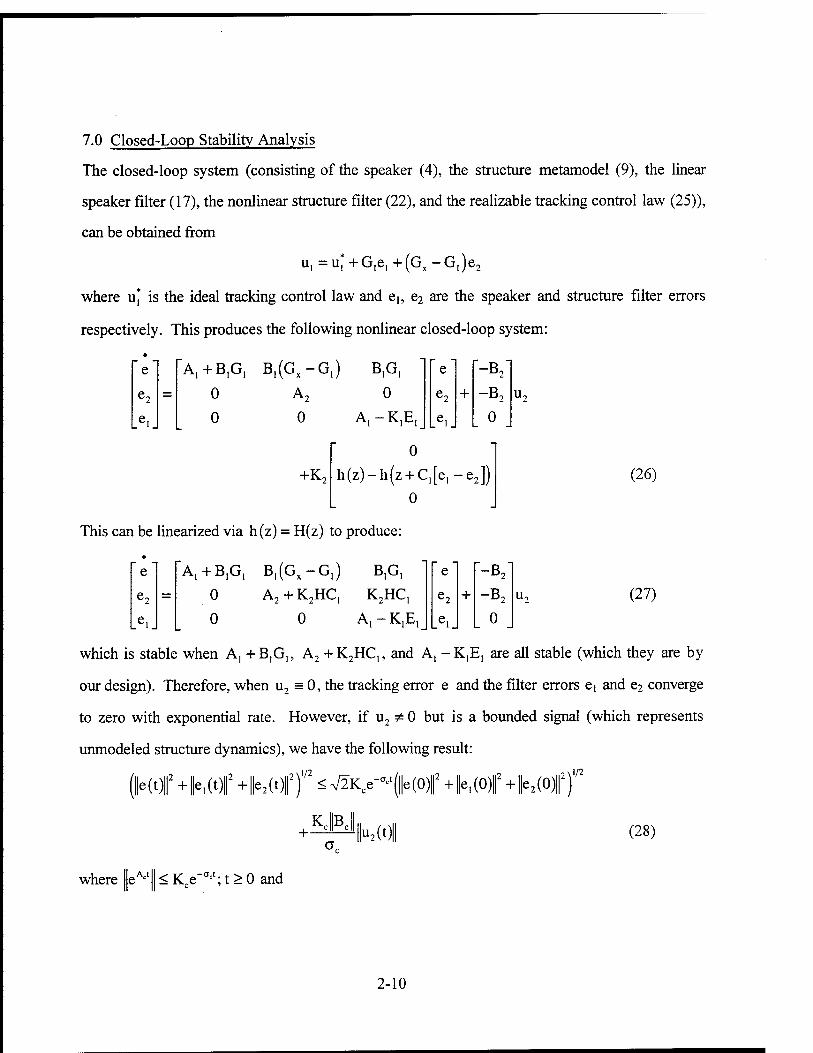
7.0 Closed-Loop Stability Analysis
The closed-loop system (consisting of the speaker (4), the structure metamodel (9), the linear
speaker filter (17), the nonlinear structure filter (22), and the realizable tracking control law (25)),
can be obtained from
u1=U;+G,e1+(Gx-GI)e2
where u| is the ideal tracking control law and ei, e2 are the speaker and structure filter errors
respectively. This produces the following nonlinear closed-loop system:
e
e,
A.+B.G, B,(GX-G,) B,G,
0
0 0
+K„
A.-K.E,
0
[~e "-B2"
e2 + -B2
Lei. i
o i
h(z)-h(z + C1[e1 -e2])
0
(26)
This can be linearized via h(z) = H(z) to produce:
e "A,+ B,G, 13,(0,-0,) B,G, e
e2 = 0 A2 + K2HC, K2HC, e2
.e>. 0 0 A,-K,E,_ _ei
-B2
-B, (27)
which is stable when A, +B,G,, A2 +K2HC,, and A, -K,E, are all stable (which they are by
our design). Therefore, when u2 = 0, the tracking error e and the filter errors ei and e2 converge
to zero with exponential rate. However, if u2 * 0 but is a bounded signal (which represents
unmodeled structure dynamics), we have the following result:
(||e(t)||2 -H||ei(t)||2 -H||e2(t)||2),/2 < V2Klce-^(||e(0)||2 + jjGl (0)f H-||e2(0)||2f
Kite
\'/2
+- 1h(t (28)
where eA<' < ICe-0'1; t > 0 and
2-10

A„ = A.+B.G, B.fG.-G,)'
0 A2 + K2HC, and Bc =
-B2
-B2 A • See Appendix for proof of (28).
0
This shows that in the limit, as t -> °° the errors e(t), e,(t), e2(t), are ultimately bounded by
K llB II ||u2(t)|. Thus, when the metamodel of the structure is actually driven by a nonzero u2(t),
6C
the best outcome is that our tracking controller will produce a bounded tracking error
proportional to |u2(t)|; otherwise, if u2(t) = 0, the tracking error converges to zero. This clearly
illuminates the difference between a perfect and an imperfect world.
7.0 Conclusions
This report details the supporting theory for a new approach to precision tracking control. A
partitioned filter method has been shown to yield stable closed-loop control of a voice-coil
actuated interferometer to track the motion of a flexible, deployable supporting structure. The
partitioned filter uses the separated signals from the actuator current and the normalized intensity
of an avalanche photodiode to produce precision control commands.
Ongoing numerical and laboratory experiments at the IGDL facility of the USAF Phillips
Laboratory are being performed to validate this approach for future space-based demonstrations.
Acknowledgments
The author is grateful for the support of AFOSR via the Summer Research Program in residence
at the USAF Phillips Laboratory, Albuquerque, NM, for the period May 15 to July 15, 1997.
My very special thanks go to the UltraLITE Team, especially Mike Powers, L. (Robbie)
Robertson, Karl Schrader, and Jesse Leitner, who made this research such an excellent experience
and the IGDL, my home away from home.
References
1. M. Powers, et al. "UltraLITE: Assessment of Lightweight, Large Aperture
2-11
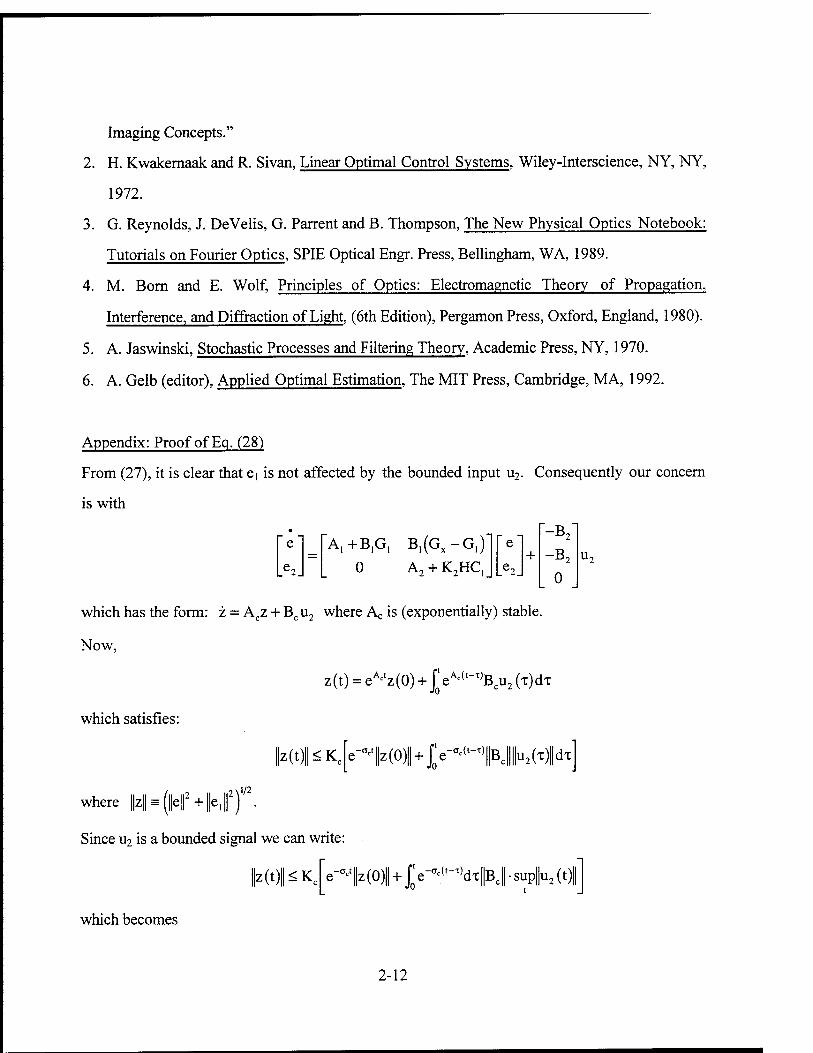
Imaging Concepts."
2. H. Kwakernaak and R. Sivan, Linear Optimal Control Systems, Wiley-Interscience, NY, NY,
1972.
3. G. Reynolds, J. DeVelis, G. Parrent and B. Thompson, The New Physical Optics Notebook:
Tutorials on Fourier Optics, SPIE Optical Engr. Press, Bellingham, WA, 1989.
4. M. Born and E. Wolf, Principles of Optics: Electromagnetic Theory of Propagation,
Interference, and Diffraction of Light, (6th Edition), Pergamon Press, Oxford, England, 1980).
5. A. Jaswinski, Stochastic Processes and Filtering Theory, Academic Press, NY, 1970.
6. A. Gelb (editor), Applied Optimal Estimation, The MIT Press, Cambridge, MA, 1992.
Appendix: Proof of Eg. (28)
From (27), it is clear that ei is not affected by the bounded input u2. Consequently our concern
is with
A.+B.G, B.fo-G,)'
0 A2 + K2HC, +
-B2
-B2
0
which has the form: z = Acz + Bc u2 where Ac is (exponentially) stable.
Now,
z (t) = e A<'z (0) + £ e Mt-T)Bcu2 (x) dx
which satisfies:
[z(t)|| < Kc[e-^|z(0)|| + jy^lBjMxIdx
/ 2 l|2\I/2
where ||z|| = f||e|| + ||ei|| ) •
Since u2 is a bounded signal we can write:
M0NKC e-CTet||z(0)j| + jYCT<(t-T,dx|Bc|| • sup||u2 (t
which becomes
2-12
|z(t)MK£ e-a1z(0)| + ^4^|Bc|sup|u2 <K, B
1|z(0)| + "sup|u2(t)| <7„ t
Because e2(t) = e(A|_K,E,)te2(0) we know we can choose K, so that |e2(t)| < Kce Cct|e2(0)||.
Therefore, using
-(iieirHhir+iKirr^iNf+hirr^iNi+iKi,
we obtain
(lief + |e,f + |e2f f < Kce^[||z(0)|| 4- ||e2(0)||] + ±f& • sup||u2(t)||
From |z(0)| + |e2(0)|| < V2(j|z(0)||2 + ||e2(0)||2)V2, we have the desired (28).
2-13
MULTIPLE APERTURE AVERAGING TECHNIQUE FOR MEASUREMENT FULL APERTURE TILT WITH A LASER GUIDE STAR AND EXPERIMENTAL
STUDY OF TILT ANGULAR ANISOPLANATISM
Mikhail S. Belen'kii Assistant Professor
Department of Philosophy
Georgia Technology Research Institute Atlanta, GA 30332
Final Report for: Summer Research Program
Phillips Laboratory
Sponsored by: Air Force Office of Scientific Research
Boiling Air Force Base, Washington, DC
And
Phillips Laboratory
September 1997
3-1
MULTIPLE APERTURE AVERAGING TECHNIQUE FOR MEASUREMENT FULL APERTURE TILT WITH A LASER GUIDE STAR AND EXPERIMENTAL STUDY OF TILT ANGULAR
ANISOPLANATISM
Mikhail S. Belen'kii Principal Research Scientist
Georgia Tech Research Institute Georgia Institute of Technology
Atlanta, GA 30332-0834
Abstract
A method for measuring full aperture tilt with a LGS is developed. The method exploits a single monochromatic LGS formed through the main telescope and uses two arrays of small auxiliary telescopes separated in orthogonal directions to view the LGS. To reduce the contribution of a down propagation path to the measured tilt, four averaging techniques are used. It is shown that the contribution of the down propagation path can be reduced by averaging a LGS image over FOV of the receiver, over the position of the auxiliary telescope in the telescope array, over position of a subaperture within the auxiliary telescope, and over time. We found that the use of the above averaging techniques permits us to achieve the Strehl ratio equal to 0.7 for various seeing conditions, different telescope diameter, and wavelength, including a visible waveband. A designing methodology for the tilt measurement scheme with a LGS is discussed. An experimental study of the tilt angular correlation scale and the tilt angular averaging function is performed. A new approach of measuring tilt angular anisoplanatism is exploited. This approach employs measurements of the random motion of the portions of a moon edge image to assess wavefront tilt. This technique provides a wide, continuous range of angular separations which are not available in observations with a binary stars. This allows measurements of the tilt averaging function. Besides, the moon is sufficiently bright to enable observations with a high resolution CCD imaging system, and, at any given site and time, the moon is more likely to be available for observations than specific binary stars. In this experiment, the statistical properties of tilt angular correlation and the tilt averaging function were studied. According to estimates based on the tilt averaging function, the tilt angular correlation scale increases by increasing the telescope diameter from 40 arcsec to 118 arcsec. This indicates that the concept of isoplanatic angle is not applicable to tilt-related phenomena. The data obtained can be used for designing the tilt measurement scheme.
3-2
MULTIPLE APERTURE AVERAGING TECHNIQUE FOR MEASUREMENT FULL APERTURE TILT WITH A LASER GUIDE STAR AND EXPERIMENTAL STUDY OF TILT ANGULAR
ANISOPLANATISM
Mikhail S. Belen'kii
Introduction The inability of a laser guide star (LGS) scheme to sense a full aperture tilt places a fundamental limitation on adaptive optics (AO) systems and limits the area of the sky accessible for AO correction. During the last few years, several different techniques for measuring tilt with a LGS were proposed. In particular, Foy et. al.{l}suggested a polychromatic LGS method with two multicolor sodium beacons. This technique uses the wavelength dependence of the index of refraction. However, for ordinary atmospheric conditions, the wavelength dependence of the index of refraction is very weak. The difference in the index of refraction only a few percent when the difference in the wavelength is about one decade, which makes implementation of this technique difficult.
Belen'kii {2} suggested the method which uses a single monochromatic LGS and two auxiliary telescopes separated from the main telescope in transverse directions. A LGS is formed by a laser beam transmitting through the main telescope and auxiliary telescopes are used to view the LGS. A tilt component corresponding to the down propagation path in this technique is eliminated by averaging a LGS image over a laser beacon angular extent. This method has several advantages. First, as opposed to the Foy et. al. technique {1}, this method is based on the first order, but not second order, effect. Second, the aperture size for an auxiliary telescope is independent ofthat for the main telescope and can be small. Third, a one- dimensional CCD array can be used to increase the signal-to-noise ratio for an auxiliary telescope because only global motion of the LGS image, as a whole, should be measured. Belen'kii {3} also suggested a tilt measurement scheme with a small aperture beam transmitted from behind a portion of a primary mirror, which does not require transmitting high power laser irradiance through the main optical train, and might be used for the mesospheric sodium layer.
Ragazzoni{4} suggested a LGS scheme with a laser beam launched through a laser projector, which has the same diameter as the main telescope and placed far away from it. The problem with this scheme is that two 8 m laser projectors are required to measure two-axis tilt components for an 8 m telescope. Besides, due to the fact that a LGS is viewed through the main telescope, a large FOV and large separations (up to 600 Km ) between the main telescope and beam projectors are required, which is far from practical. Another scheme suggested by Ragazzoni {5}uses time delay effect for the sodium beacon. However, the propagation time delay for the LGS at the altitude If= 90 Km is X = 6-10^ S. Whereas, the tilt temporal correlation scale for the telescope of diameter D> 1.5 m, according to the measured data {6} is larger than tc> Is. Therefore, the ratio X / tc is less than x/ /,<6 • 10~ . The implication is that expected LGS image motion is small, and the required measurement accuracy is far beyond the capability of current optical sensors.
Even though the LGS techniques suggested in {2,3} do not have the above shortcomings, they, nevertheless, require large FOV and large separations between the main and auxiliary telescopes to achieve the Strehl ratio (SR), which are needed for practical AO systems. In the paper by Belen'kii {7}, a general approach for measuring tilt with a LGS was presented. This approach uses a single LGS and two arrays of auxiliary telescopes placed in orthogonal directions. Angular, spatial, temporal, and multiple aperture averaging techniques are exploited to reduce the tilt component corresponding to the down propagation path. This permits us to diminish FOV of the receiver and the distance between the main telescope and auxiliary telescope array.
Description of principle
A bistatic LGS scheme suggested in Ref. 2 is shown in Fig. 1. A laser beacon formed through the main telescope is observed through an auxiliary telescope. An auxiliary telescope sees a beacon as an extended
3-3
object. Light emitted from different portions of the LGS pass through different inhomogeneities, due to the fact the LGS image appears wavy. A waviness scale is determined by the tilt angular correlation scale, 0 t, which is proportional to auxiliary telescope diameter {3,8}. A tilt component corresponding to the down propagation path is eliminated by averaging randomly different motion of the portions of a LGS image over a laser beacon angular extent. To obtain the required amount of averaging, FOV of the receiver, 9 K, should greatly exceed the tilt angular correlation scale, 0 /. The estimates {3,8} show that even for a small aperture telescope, a tilt angular correlation scale is tens of arcsec. As a result, large FOV and large separations, A , are needed to measure tilt. A modification of this technique considered below simplifies the requirements of the measurement scheme.
An analysis of a LGS scheme shown in Fig. 1 reveals that integration of a LGS image over FOV of the receiver is not the only way to reduce the contribution of a down propagation path. Indeed, the tilt measured with the auxiliary telescope consists of two components,
(p(0,i?^=cp^(^ + (p^(0,7?/). (1)
The first component, (p LB, is the full aperture tilt for the transmitted beam which corresponds to the upward propagation path. The second component, cp DJK is the tilt resulting from the down propagation path. There are several fundamental differences between these tilt components. First, the tilt component cp Dp depends on angle 0 and has randomly different values in different directions, whereas the tilt component cp ^ is independent of 0 . Second, the tilt component, cp 'Dp, depends on the spatial position of the receiving telescope, Ä, whereas the tilt component, (p Lb, is independent of R. Finally, both components, (p ^ and (p Dp> depend on time, /. However, if the diameter of the main telescope greatly exceeds that for an auxiliary telescope, its tilt temporal correlation scale is much greater than that for the auxiliary one. All these differences can be used to reduce the contribution of the down propagation path, cp Dp, to the measured tilt. Let us assume that an array of A auxiliary telescopes separated from each other at the distance, A ,, are
used to measure tilt. Each telescope in the array, as shown in Fig. 2, is pointed at the LGS. Let us also assume the LGS image is integrated over FOV of the receiver, 0 R, over position of an auxiliary telescope in the array, and over time, 7, which is much smaller than the tilt temporal correlation scale for the component cp ^ corresponding to the transmitted beam, T« tjj... The integrated LGS tilt is given by
1 e* 1 N 1 T
ö R 0 /V>1 J 0
By assuming that angular, spatial, and temporal coordinates are statistically independent, one can estimate 1-2 \ variance of the integrated tilt, yep ASr/. It should be noted that motion of the turbulent inhomogeneities
due to wind does not affect statistical independence of the spatial and temporal coordinates. Indeed, if the separation is A j «10 IL, then for a sodium beacon ( H— 90 jfaz) at the altitude H= 10 Jar. the distance between the propagation paths for two auxiliary telescopes is about 9 m. For wind velocity V= 10 ml s and integration time T< 0.1S, displacement of inhomogeneities is less than 1 JTJ, which is much smaller than the distance between the propagation paths. Variance of the integrated tilt equals
\<?24Sr) = \<?2iJl+°2w (3) / 2 \ 2
Here \Cp LB/ is the tilt variance for the transmitted beam, and a DP is the tilt variance for the down
propagation path.
3-4
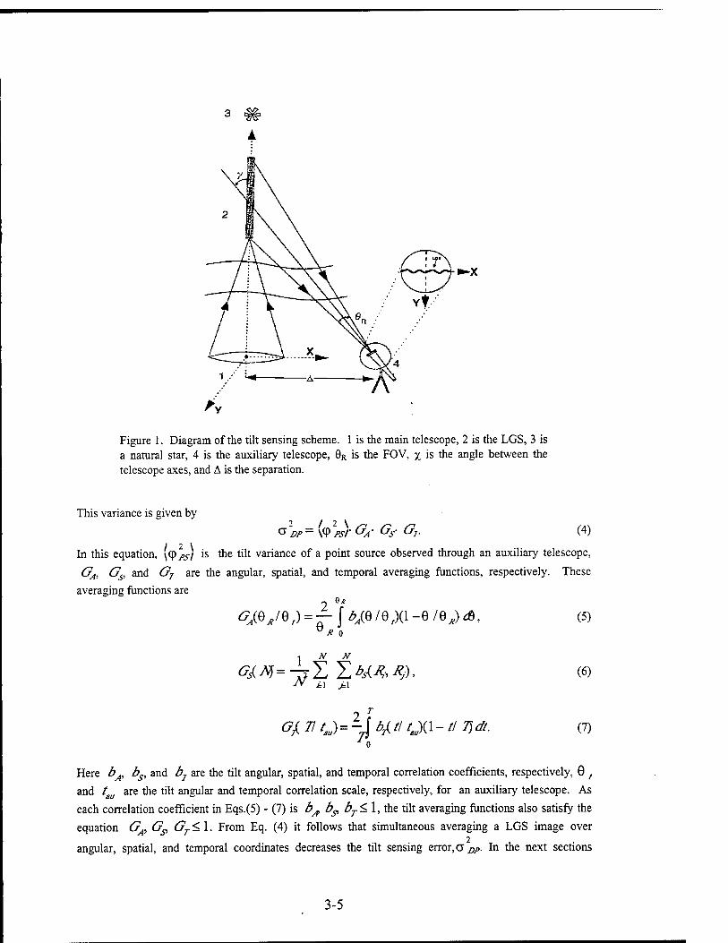
Figure 1. Diagram of the tilt sensing scheme. 1 is the main telescope, 2 is the LGS, 3 is a natural star, 4 is the auxiliary telescope, 9R is the FOV, % is the angle between the telescope axes, and A is the separation.
This variance is given by
/ 2 \
^'DP- \<?PS/- G
A- <%• GJ- (4)
In this equation, \(pj>s/ is the tilt variance of a point source observed through an auxiliary telescope,
GA, Gs, and GT are the angular, spatial, and temporal averaging functions, respectively. These averaging functions are
e* ^(0/0,) = — {^(e/e.xi-e/e^rf),
" R 0
(5)
(6)
(7)
Here bA, bs, and by are the tilt angular, spatial, and temporal correlation coefficients, respectively, 0 , and t are the tilt angular and temporal correlation scale, respectively, for an auxiliary telescope. As
each correlation coefficient in Eqs.(5) - (7) is bA b^ bT<\, the tilt averaging functions also satisfy the equation GA, G^ GT<\. From Eq. (4) it follows that simultaneous averaging a LGS image over
2 angular, spatial, and temporal coordinates decreases the tilt sensing error, <5 DP. In the next sections
3-5
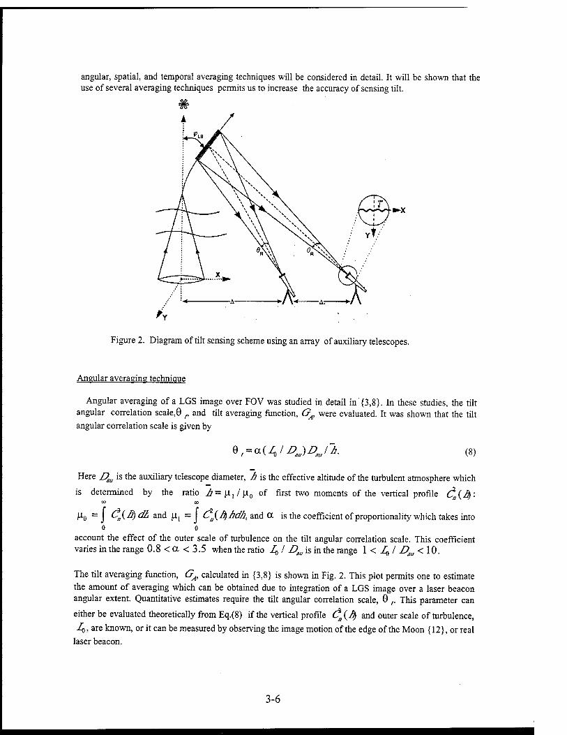
angular, spatial, and temporal averaging techniques will be considered in detail. It will be shown that the use of several averaging techniques permits us to increase the accuracy of sensing tilt.
*-x
Figure 2. Diagram of tilt sensing scheme using an array of auxiliary telescopes.
Angular averaging technique
Angular averaging of a LGS image over FOV was studied in detail in {3,8}. In these studies, the tilt angular correlation scale,G r and tilt averaging function, GA, were evaluated. It was shown that the tilt angular correlation scale is given by
§ =o.{I^I DJDJ h. (8)
Here Dau is the auxiliary telescope diameter, h is the effective altitude of the turbulent atmosphere which
is determined by the ratio J}=\lxl\l0 of first two moments of the vertical profile Ö„(ß): 00 00
M-o =J ^(-^^ and |a, = j Cn{J^Jidh,2x\AO. is the coefficient of proportionality which takes into o o
account the effect of the outer scale of turbulence on the tilt angular correlation scale. This coefficient varies in the range 0.8 < a < 3.5 when the ratio 1$ I Dau is in the range 1 < 1^ I Dau < 10.
The tilt averaging function, GA, calculated in {3,8} is shown in Fig. 2. This plot permits one to estimate the amount of averaging which can be obtained due to integration of a LGS image over a laser beacon angular extent. Quantitative estimates require the tilt angular correlation scale, 9,. This parameter can
either be evaluated theoretically from Eq.(8) if the vertical profile £?(4 and outer scale of turbulence, Zc, are known, or it can be measured by observing the image motion of the edge of the Moon {12}, or real
laser beacon.
3-6
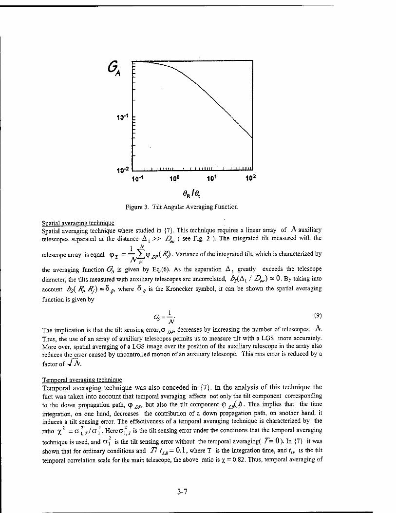
ej6x
Figure 3. Tilt Angular Averaging Function
Spatial averaging technique Spatial averaging technique where studied in {7}. This technique requires a linear array of A auxiliary telescopes separated at the distance A, » Dau ( see Fig. 2 ). The integrated tilt measured with the
telescope array is equal 1 N
N% (ty . Variance of the integrated tilt, which is characterized by
the averaging function Gs is given by Eq.(6). As the separation A, greatly exceeds the telescope
diameter, the tilts measured with auxiliary telescopes are uncorrelated, bJ^Lx I Dsu) « 0. By taking into account bj^ Rf, RJ) = 5 ,y, where 5 ^ is the Kronecker symbol, it can be shown the spatial averaging
function is given by
Gs = N (9)
The implication is that the tilt sensing error, a Dfn decreases by increasing the number of telescopes, A. Thus, the use of an array of auxiliary telescopes permits us to measure tilt with a LGS more accurately. More over, spatial averaging of a LGS image over the position of the auxiliary telescope in the array also reduces the error caused by uncontrolled motion of an auxiliary telescope. This rms error is reduced by a
factor of J~Ä.
Temporal averaging technique Temporal averaging technique was also conceded in {7}. In the analysis of this technique the fact was taken into account that temporal averaging affects not only the tilt component corresponding to the down propagation path, (p DJ» but also the tilt component (p ^ i). This implies that the time integration, on one hand, decreases the contribution of a down propagation path, on another hand, it induces a tilt sensing error. The effectiveness of a temporal averaging technique is characterized by the ratio %2 = G \ rl<3 f. Here a,2 7 is the tilt sensing error under the conditions that the temporal averaging
technique is used, and CT, is the tilt sensing error without the temporal averaging( T= 0). In {7} it was shown that for ordinary conditions and Tl tLB=Q.\, where T is the integration time, and tu is the tilt temporal correlation scale for the main telescope, the above ratio is % = 0.82. Thus, temporal averaging of
3-7
a LGS image can be used along with spatial and angular averaging, to increase the accuracy of measurement of a full aperture tilt.
<
Strehl ratio estimation
The performance of AO systems is characterized by the Strehl ratio. This ratio for tilt error is give by {9,10}
SX= 2 , (9)
2 \l D
where a, is the one-axis, rms, tilt sensing error, X is the wavelength, and £, is the main telescope I 2\1/2
diameter. The tilt sensing error rms is determined by the equation G, = \((p — (p NJ) / , where (p is the
tilt measured with a LGS, and (p NS is the full aperture tilt for a natural star measured with the main
telescope. The Strehl ratio given by Eq.(9) is equal SR= 0.7 if the ratioCT] /(X ID) is ü] /(k I D) = 0.3. Parameters of AO systems, which are needed to achieve the Strehl ratio SR= 0.7
for good (JQ - 0.2 m at X=0.55 urn) and poor (JQ — 0.07/2: at X=0.55 \xm) seeing conditions were
estimated in {7}. For a site with good seeing conditions, such as Mauna Kea {11}, r0 = 0.235 m, an auxiliary telescope of diameter Dau = 0.3 m was considered. For r0 = 0.235 m, 1^ = 6 /£, and
Dau = 0.3 m the image jitter rms of the point sources estimated from Eq.(15) is (<p„2) = 0.18 arcsec. The
number of auxiliary telescopes, N, which are required to achieve the Strehl ratio SR = 0.7 for one-axis tilt component for a 8 m telescope and A=2.2 \xm for the above conditions is presented in Table 1.
Table 1. Number of Auxiliary Telescopes Needed to Achieve a Strehl Ratio of 0.7 for One-axis Tilt Component with Sodium Beacon at the Site with Good Seeing Conditions
D = Sm,X = 2.2 \xm,Dm = 0.3 m, SR = 0.7
eR 6 mrad 3 mrad 1.5 mrad N(T=0) 5 8 13
N(T/t,K = 0.1) 3 5 10
We see that only from 3 to 5 auxiliary telescopes with FOV from 6 mrad to 3 mrad are needed to achieve the Strehl ratio SR=0.7 for one -axis tilt component a 8 m telescope at Mauna Kea . For the larger FOV, a smaller number of telescopes are required. To assess another wave front tilt component an additional telescope array orthogonal to the first array should be used.
For poor seeing conditions, ^ = 0.07A, corresponding to the Starfire Optical Range at Kirtland Air
Force Base in Albuquerque, NM, an auxiliary telescope of diameter Dau = 0.2 iz with FOV B = 6 mrad
was considered. For a Rayleigh beacon (10km± 2km) and FOV of 8„= 6 mrad, the separation between the main telescope and the array of auxiliary telescopes is A=300 m. The estimated number of auxiliary telescopes, N, needed to achieve the Strehl ratio SR=0.7 for one-axis tilt component and the above conditions is given in Table 2. For a 1.5 m telescope, the estimates are obtained without using the temporal averaging (T = 0), whereas for a 3.5 m telescope, the temporal averaging is exploited.
It is seen that for a 1.5 m telescope and near IR waveband from 3 to 9 telescopes are needed to achieve the Strehl ratio SR=0.7. At the same time, in the visible range, a much large number of telescopes are required. This means that a tilt measurement scheme should be further improved. One more averaging technique uses averaging of a LGS image over subaperture position within an auxiliary telescope.
3-8
Table 2. Number of Auxiliary Telescopes Needed to Achieve Strehl Ratio of 0.7 of One- axis Tilt Component with Rayleigh Beacon at the Site with Poor Seeing Conditions
e„ = 6 mrad, Dau = 0.2 m. A = 300 m, SR = 0.7
X \\im\ 2.2 1.25 0.55
N(D = 1.5m, T=0) 3 9 50
N(D = 3.5m, T/t,„ = 0.1) 12 35 --
Multiple aperture averaging technique
Let us assume that an auxiliary telescope consists of multiple subapertures. If subaperture diameters Dm„ then the tilt angular correlation scale for a LGS image formed by each subaperture is determined by Dm, providing effective averaging over the angular coordinate. At the same time, when LGS images are
averaged over multiple subapertures the jitter variance of a point source \(P/>y/ decreases. If each auxiliary
telescope of diameter DT consists of M subapertures of diameter £>„„, where M= Dz'/Dj, than the LGS tilt measured with each subaperture, cp, can be averaged over multiple subapertures within an auxiliary
' 1 M
telescope. The integrated tilt measured with auxiliary telescope is cp = ~3_,(p_/- In this case, the LGS
tilt integrated over angular, spatial, and temporal coordinates is given by 1 M 1 e* 1 N 1 *
<P A ST, MA
where R is the subaperture coordinate within an auxiliary telescope. Variance of the integrated LGS tilt has the form
CT DP = \9 psf GA Gs GT'
GMX (11)
where GMA is the averaging function due to averaging of the LGS image over subapertures within an auxiliary telescope. The number of auxiliary telescopes which are required to achieve the SR=0.7 for the same conditions as Table 2 calculated in {7} are presented in Table 3. In this case, a multiple aperture averaging technique is used. The auxiliary telescope diameter is Dz=0.5m, and the subaperture diameter is Da=0.2m. The number of auxiliary telescopes decreases approximately by a factor of three if a multiple aperture averaging technique is exploited. A similar reduction factor can also be obtained for the case of a sodium beacon presented in Table. 1. Thus, only from 4 to 12 multiple aperture auxiliary telescopes are needed to achieve SR = 0.7 for a 3.5 m telescope in near ER..
Table 3. Number of Auxiliary Telescopes Needed to Achieve Strehl Ratio of 0.7 with Rayleigh Beacon and Multiple Aperture Averaging at a Site with Poor Seeing Conditions
DT = 0.5 m, QR = 6 mrad, Dau = 0.2 m, A = 300 m SR = 0.7
kflimj 2.2 1.25 0.55
N(D = 1.5m,T=0) 1 3 18 N(D = 3.5m,T/t,„ = 0.1) 4 12 60
Thus, by using a combination of averaging techniques the SR=0.7 can be achieved for various seeing conditions, wide range of telescope diameter, and wavelength, including a visible waveband.
Design methodology for tilt measurement scheme
3-9
Information needed for designing the tilt measurement scheme with a LGS can be obtained in two ways. First, three basic parameters, r„, 0,, and La, needed for the system design can be measured directly. The r0
data are usually available at astronomical sites. The outer scale of turbulence, L0, can be determined from the dependence of the tilt variance on the telescope diameter {6}. The tilt angular correlation scale.0,, or the tilt angular averaging function, GA, can be measured by observing the edge of the Moon {12}. By knowing the above characteristics, one can estimate for a given main telescope diameter, £>, wavelength, X, auxiliary telescope diameter, Dm, and FOV, 9„, the angular averaging function, G4, and the number of auxiliary telescopes, N, which are needed to achieve the required Strehl ratio. If it is necessary, a complex auxiliary telescope aperture consisting of multiple subapertures can be used.
A second way is to measure the tilt sensing error a, = ((«p-cp^2/ "by observing a real laser beacon
through a single aperture auxiliary telescope. The main telescope could be pointed at Polaris to eliminate mechanical motion, and the LGS is observed through an auxiliary telescope with given diameter and FOV. By measuring Polaris motion with the main telescope and LGS motion with the auxiliary telescope, the tilt sensing error CT, can be estimated. If the error, caused by focus anisoplanatism, aF4, is small, the measured tilt error corresponds to a, = (cp^J • GA ■ By comparing the measured value a, with the ratio
DA, one can determine the number of auxiliary telescopes which are needed to achieve the required Strehl ratio.
Experimental study of tilt angular anisoplanatism
The performance of the above method of sensing full aperture tilt can be evaluated if the tilt angular correlation scale or tilt angular averaging function are known. Besides, to determine the optimum diameter of an auxiliary telescope , the tilt angular correlation scale or tilt averaging function should be known. However, these data are not available in the literature.
Thegoal of this experiment is to investigate the statistical properties of wave-front tilt angular correlation and tilt averaging function for various telescope diameter. Typically, the dependence of wave-front aberrations, which include tilt and higher-order wave-front components, on the direction of propagation of an optical wave is referred to as anisoplanatism {13}. The traditional approach for measuring tilt anisoplanatism uses binary stars at various angular separations {14,15}. However, bright binary stars with the required angular separations may not always be visible at a particular site and time, making this approach difficult to reliably implement.
A different approach, which avoids the above difficulty, is suggested in this paper. Rather than measuring the motion of binary stars at fixed angular separations, the random angular motion of an image of the moon's edge is recorded. This approach offers several advantages. First, at any given site and time the moon is more likely to be available than specific binary stars. Second, unlike binary stars, with a limited range of discrete separations, moon edge observations provide a wide and continuous range of angular distances. Third, the determination has been made that the moon's brightness is sufficient to make measurements with a high resolution CCD imaging system. This approach was employed in a recent experiment conducted at the Starfire Optical Range (SOR).
Because the Moon is an extended, incoherent source, light rays emitted from different portions of its edge travel through different inhomogeneities, causing images of the moon's edge to appear wavy. It is reasonable to expect the waviness scale of the image to be related to the area of the sky over which phase fluctuations are correlated, defined as the isoplanatic angle {13}, G„. This angle is given by
e0=(2.9i/|4(^/3^-3/5, (i2)
3-10
where K=27I/X is the wavenumber, and C; is the refractive index structure characteristic. The isoplanatic angle thus depends on wavelength, but not telescope diameter.
However, in {2} a different angular scale, known as the tilt angular correlation scale, appeared in the analysis. This scale is independent of wavelength, but it depends on telescope diameter, D, and also depends on the outer scale of turbulence. Further investigation {3.8} showed that the waviness scale of an extended incoherent object is determined not by isoplanatic angle, but by the tilt angular correlation scale, which has the form
0, =a(L0/D)D Ih. (13)
Estimates show that the effective altitude of the turbulent atmosphere is h= 934 m for the HV 57 model
corresponding to the SOR site and 2=6100 m for the C„ (ß) vertical profile corresponding to Mauna Kea
{11}. The values of a lateral (transverse to angular separation, 0 ) tilt angular correlation scale,0 ,, are
given in Table 1 in {3,8}. An additional goal of this study was to verify that the waviness scale of the moon edge is determined by wave-front tilt correlation, but not by isoplanatic angle.
Experimental set up. data collection, and data processing procedures
In this study, an experimental setup similar to that used for the Polaris jitter observations {6} was used. A diagram of the system is shown in Fig.4.
Data Frame with Image of Moon Edge
CCD
MAC
K-Mirror Moon 1.5 m Telescope
Aperture Wheel at Pupil
Figure 4. Moon Edge Jitter Experimental Setup
LL 64x64 Fast CCD Camera
256 M RAM Data Storage Computer
A 1.5 m telescope with aperture masks providing additional effective apertures of 0.1, 0.2, 0.5, and 0.75 m was used. Moon edge images were recorded with a Lincoln Laboratory fast, low noise, high resolution CCD camera (maximum 2 kHz frame rate, 10 photoelectrons/pixel/read noise, 64x64 array, and 27 um pixel size). In observations performed in 1995 an angular pixel scale of 0.9 arcsec/pixel (58x58 arcsec FOV) was used. In this case, no control over image orientation was available, so the orientation of moon edge images was arbitrary. In observations performed in 1996, a pixel scale of 0.66 arcsec/pixel (42x42 arcsec FOV) was used. In this case, a small K-mirror was employed to orient the FOV such that the moon edge was normal to the pixel rows, simplifying data post-processing.
Short exposure images of the moon were collected at a frame rate of200//z (5 ms exposures) for 100 sec or 400 Hz ( 2.5 ms exposures) for 50 sec. 20,000 frames were collected per data run. Sets of five data runs, one for each aperture, were collected sequentially. Neutral density filters were used to keep transmitted flux approximately constant. In each run (1996 experiment) the image was aligned to place the moon edge approximately near the 32nd (center) pixel in each row. In addition, for each data run, sky background and dome flat frames were collected. On average, an entire data set, including five apertures, backgrounds, and flats, was recorded in 30 min. The moon edge images were recorded during one night in August of 1995, and during four nights in May, June, and August of 1996. The atmospheric coherence diameter (r0), wind speed, and wind direction near the telescope were recorded as well. During the observations, the coherence diameter was in the range 5-9 cm.
3-11
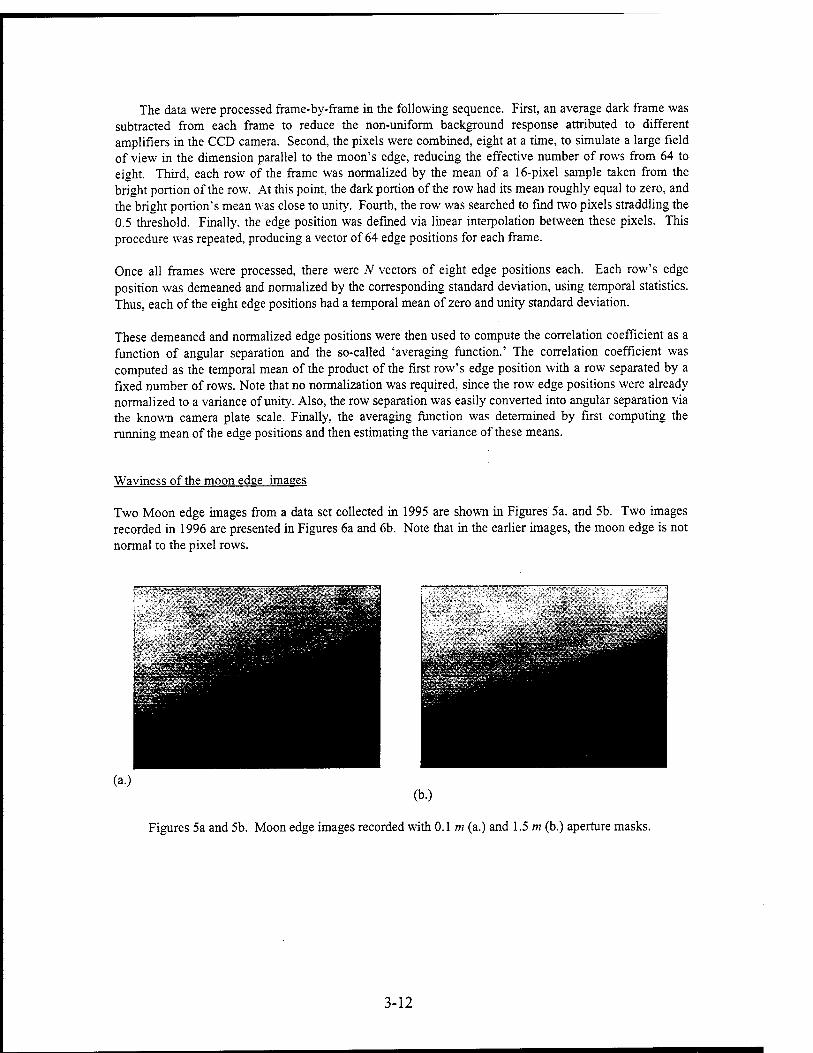
The data were processed frame-by-frame in the following sequence. First, an average dark frame was subtracted from each frame to reduce the non-uniform background response attributed to different amplifiers in the CCD camera. Second, the pixels were combined, eight at a time, to simulate a large field of view in the dimension parallel to the moon's edge, reducing the effective number of rows from 64 to eight. Third, each row of the frame was normalized by the mean of a 16-pixel sample taken from the bright portion of the row. At this point, the dark portion of the row had its mean roughly equal to zero, and the bright portion's mean was close to unity. Fourth, the row was searched to find two pixels straddling the 0.5 threshold. Finally, the edge position was defined via linear interpolation between these pixels. This procedure was repeated, producing a vector of 64 edge positions for each frame.
Once all frames were processed, there were N vectors of eight edge positions each. Each row's edge position was demeaned and normalized by the corresponding standard deviation, using temporal statistics. Thus, each of the eight edge positions had a temporal mean of zero and unity standard deviation.
These demeaned and normalized edge positions were then used to compute the correlation coefficient as a function of angular separation and the so-called 'averaging function.' The correlation coefficient was computed as the temporal mean of the product of the first row's edge position with a row separated by a fixed number of rows. Note that no normalization was required, since the row edge positions were already normalized to a variance of unity. Also, the row separation was easily converted into angular separation via the known camera plate scale. Finally, the averaging function was determined by first computing the running mean of the edge positions and then estimating the variance of these means.
Waviness of the moon edge images
Two Moon edge images from a data set collected in 1995 are shown in Figures 5a. and 5b. Two images recorded in 1996 are presented in Figures 6a and 6b. Note that in the earlier images, the moon edge is not normal to the pixel rows.
ft&S&p&gÜgff! ■ /" v*' ■ v"1"^*"" ->.'• j-jgW" "1 ;.-•■ ■ , . i 'J£#:0- '*«•';' "£flRfc-""'3|
. . '*" «•»»!.
» ■ V-'V^.^VVTW'WSJMHH
Il^^s-'^W-; ̂ f^^^^^P ■*" ' ^^äii ̂ &j£jB3
IAS^^IJSQ frffwaaff* j^ggS
SM
(a.) (b.)
Figures 5a and 5b. Moon edge images recorded with 0.1 m (a.) and 1.5 m (b.) aperture masks.
3-12
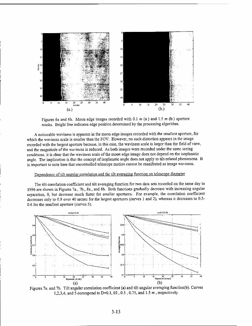
15 20 25 30 35 40 Arcs«
(a.)
Figures 6a and 6b. Moon edge images recorded with 0.1 m (a.) and 1.5 m (b.) aperture masks. Bright line indicates edge position determined by the processing algorithm.
A noticeable waviness is apparent in the moon edge images recorded with the smallest aperture, for which the waviness scale is smaller than the FOV. However, no such distortion appears in the image recorded with the largest aperture because, in this case, the waviness scale is larger than the field of view, and the magnitude of the waviness is reduced. As both images were recorded under the same seeing conditions, it is clear that the waviness scale of the moon edge image does not depend on the isoplanatic angle. The implication is that the concept of isoplanatic angle does not apply to tilt-related phenomena. It is important to note here that uncontrolled telescope motion cannot be manifested as image waviness.
Dependence of tilt angular correlation and the tilt averaging function on telescope diameter
The tilt correlation coefficient and tilt averaging function for two data sets recorded on the same day in 1996 are shown in Figures 7a., 7b., 8a., and 8b. Both functions gradually decrease with increasing angular separation, 8, but decrease much faster for smaller apertures. For example, the correlation coefficient decreases only to 0.8 over 40 arcsec for the largest apertures (curves 1 and 2), whereas it decreases to 0.5- 0.6 for the smallest aperture (curves 5).
15 20 25 30 35 Separation [arcsec]
■^"vX. :
" -2
10 15 20 25 Separation [arcsec]
(a) (b) Figures 7a. and 7b. Tilt angular correlation coefficient (a) and tilt angular averaging function(b). Curves
1,2,3,4, and 5 correspond to D=0.1, 02., 0.5 , 0.75, and 1.5 m, respectively.
3-13
(a) (b) Figures 8a. and 8b. Tilt angular correlation coefficient (a) and tilt angular averaging function(b). Curves
1,2,3, and 5 correspond to D=0.1, 02., 0.5 , and 1.5 m , respectively.
By comparing the tilt correlation coefficients presented in Fig.7a with universal theoretical curve for tilt correlation coefficient given in Fig.3 in Ref. 6, the tilt correlation scale, 9,, can be estimated. This scale equal 6,= 54 arcsec for D=0.lm, Q = 74 arcsec for D= 0.2m , and 6,= 152 arcsec for D= 0.5m -1.5m. At the same time, by comparing the measured tilt averaging functions, given in Fig.3b with the theoretical prediction shown in Fig.2 in Ref. 9, it can be obtained that the tilt correlation scale is 9,= 38 arcsec for D-O.lm, 9,= 43 arcsec for D= 0.2m, and 0,= 118 arcsec for D= 0.5m -1.5m. The inverse order of the curves for the largest apertures in Figs. 3a. and 3b. is most likely due to atmospheric instability over the period of data collection for the five apertures.
By performing similar analysis for the data presented in Pigs. 8a, the following estimates for the tilt correlation scale can be obtained: G,= 70 arcsec for D=0.\m, 9,= 116 arcsec for D= 0.5m , and 0,= 175 arcsec for£»= 0.75/n -1.5m. The estimates obtained from the tilt averaging functions given in Fig.4b are 0,= 40 arcsec for D=0.1m, 0,= 88 arcsec for D= 0.5m , and 9,= 116 arcsec for D= 0.15m -1.5m. It is seen that., the estimates obtained from the tilt correlation coefficient exceed that inferred from the tilt averaging function. The estimates for 9, obtained from the tilt averaging function for two data sets are in better agreement than that inferred from the tilt correlation coefficient. Because the tilt averaging function, due to definition, characterizes the reduction in the tilt variance which can be obtained by integrating the image over the FOV of the receiver, the estimates for 0, inferred from these data are more suitable for estimating the performance of the LGS tilt measurement scheme {2,7}.
The estimates for the tilt angular correlation coefficient, on average, are somewhat less than that predicted by the HV in turbulent model ( see Table. 1 in {3,8}). In particular, for the largest aperture, D=1.5 m , the tilt correlation scale in the range 255- 323 arcsec was predicted, whereas the measured tilt correlation scale for this aperture is 0, < 152 arcsec. This indicates the presence of high altitude turbulence which is not accounted for by this model. Finally, the obtained change of the waviness scale of the moon edge image with variation of the telescope diameter provides clear evidence that the concept of isoplanatic angle is not applicable to tilt-related phenomena.
Conclusions
A method for measuring full aperture tilt with a LGS is developed. The method uses a single monochromatic LGS formed through the main telescope and two arrays of auxiliary telescopes separated in orthogonal directions. Four averaging techniques are applied to a LGS image to reduce the contribution of a down propagation path. A LGS image is averaged over the position of the auxiliary telescope in the telescope array, over position of a subaperture within the auxiliary telescope, over FOV of the receiver, and over time. It is shown that the use of a combination of four averaging techniques permits us to achieve the
3-14
Strehl ratio equal to 0.7 for various seeing conditions, different telescope diameter, and wavelength, including a visible waveband. A designing methodology for the tilt measurement scheme with a LGS is discussed. An experimental verification of this method should be the next step in development of a tilt retrieval technique with a LGS. An experimental study of the tilt angular correlation scale and the tilt angular averaging function was also performed as a part of the project. A new approach of measuring tilt angular anisoplanatism is exploited. This approach employs measurements of the random motion of the portions of a moon edge image in the direction transverse to the image. This technique has several advantages over the traditional method of using binary stars. They are the following: a) moon edge observations provide a wide, continuous range of angular separations which permits us to measure tilt averaging function directly; b) the moon is sufficiently bright to enable observations with a high resolution CCD imaging system; c) at any given site and time the moon is more likely to be available for observations than specific binary stars. In this experiment, the statistical properties of tilt angular correlation and the tilt averaging function were studied. According to estimates based on the tilt averaging function, the tilt angular correlation scale increases by increasing the telescope diameter from 40 arcsec to 118 arcsec. This indicates that the concept of isoplanatic angle is not applicable to tilt-related phenomena. The data obtained can be used for designing the tilt measurement scheme.
References
1. R. Foy. A Migus, F. Biraben, G. Grynberg, P.R. MsCulough, and M. Tallon, "The polychromatic artificial Sodium star: a new concept for correction the atmospheric tilt," Astron. Astrophys., Ill, 569- 578(1995).
2. M. S. Belen'kii, "Full aperture measurement technique with a laser guide star," in Annospheric Propagation and Remote Sensing IV. J. Christopher Dainty, Editor, Proc. SPJE, 2471, 289-300(1995).
3. M. S. Belen'kii, "Tilt angular correlation and tilt sensing techniques with a laser guide star," in Optics in Atmospheric Propagation. Adaptive Systems, and Lidar Techniques for Remote Sensing. Proc. EUROPTO Series, 2956, 206-217 (1996).
4. R. Raggazzoni, "Absolute tip-tilt determination with laser beacons," Astron. Astrophys. 305, L13- L16(1996).
5. R. Raggazzoni, "Propagation delay of a laser beacon as a tool to retrieve absolute tilt measurements," Astrophys. J. 465: L73-L75 (1996).
6. M. S. Belen'kii, S. J. Karis, J. M. Brown, and R. Q. Fugate, "Experimental study of the effect of non- Kolmogorov turbulence on star image motion/Woe. SPIE, 3126, (1997) (to be published).
7. M. S. Belen'kii,"Multiple aperture averaging technqiue for measuring full aperture tilt with a laser guide star," Proc. SPIE, 3126, (1997) (to be published).
8. M. S. Belen'kii, "Principle of equivalency of the phase difference and off-axis tilt sensing technique with a laser guide star," Proc. SPIE, 2828, 280-292 (1996).
9. G. A Tyler, "The reduction in antenna gain due to random jitter," the Optical Science Company Technical Report No. TR-541, Anaheim, (1983).
10. D. G. Sandler, S. Stahl, J. R. P. Angel, M. Lloyd-Hart, and D. McCarthy, "Adaptive optics for diffraction-limited infrared imaging with 8-m telescopes," J. Opt. Soc. Am., A 11, 925-945(1994).
U.R. Racine and B. L. Ellerbroek, "Profiles of night-time turbulence above Mauna Kea and isoplanatism extension in adaptive optics," SPIE Proc. 2534, 248-257 (1995).
12. M. S. Belen'kii, S. J. Karis, J. M. Brown, and R. Q. Fugate, " Measurements of tilt angular anisoplanatism," Proc. SPIE, 3126, (1997) (to be published).
13. D. L. Fried, "Anisoplanatism in adaptive optics," J. Opt. Soc. Am., 72, 52-61(1982). 14. A. Sivaramakrihnan, R. J. Weymann, and J. Beletic, "Measurements of the angular correlation of
stellar centroid motion," Astron. J., 110,430-438(1995). 15. K. Berkelfeld and A. Glideenmann, "Measurements of the isoplanatic angle of the wavefront tilt,"
Summaries of the papers presented at the topical meeting. Adaptive Optics, Maui, Hawaii, 8-12 July 96, pp206-208.
3-15
SPINNING HOLLOW FIBERS FROM HIGH PERFORMANCE POLYMERS
Gajanan S. Bhat Associate Professor-Textile Science
University of Tennessee 230 Jessie Harris Building
Knoxville, TN 37996
Final Report for: Summer Faculty Research Program
Phillips Laboratory
Sponsored by: Air Force Office of Scientific Research
Boiling Air Force Base, DC
and
Phillips Laboratory
August 1997
4-1
SPINNING HOLLOW FIBERS FROM HIGH PERFORMANCE POLYMERS
Gajanan S. Bhat Associate Professor-Textile Science
Abstract
Hollow fibers spun from synthetic polymers have been investigated for a long time,
especially for producing high-bulk, low density fabrics. Advantages of hollow fibers over solid
round fibers are improved thermal and acoustical properties, reduced pilling, special optical effects
and greater dielectric strength. Also, hollow fibers exhibit less fibrillation tendency under flexing
conditions. Such fibers produced from a high temperature resistant polymer have advantages in some
of the intended applications. A special set-up was built at the Phillips Laboratory of Edwards AFB,
CA to spin hollow fibers. Using that set-up, hollow fibers were spun from two grades of Ultem. The
same set-up was used to obtain thick coating of Ultem on copper wires. Influence of varying some
of the processing conditions on the fiber structure was analyzed. Feasibility of solution processing
of Ultem was also investigated.
4-2

SPINNING HOLLOW FIBERS FROM HIGH PERFORMANCE POLYMERS
Gajanan S. Bhat
BACKGROUND
Polyimide is a high temperature resistant polymer with excellent mechanical properties. Polyimide
fibers have excellent thermal and chemical stability and good mechanical properties as well [1, 2].
The very fact that they have good chemical stability means, they neither dissolve in simple solvents
nor melt, and this creates problem for fabrication of products. Copolyimides on the other hand have
better tractability and can be dissolved in less exotic solvents. Some of the copolyimides have been
tried for the production of fibers and other products due to the ease of fabrication. One such example
is the P84 fiber manufactured and marketed by Lenzing Co., Austria, from the 80/20 copolymer
produced by Dow Chemical Company [3]. However, even this fiber is partially crosslinked and thus
can be dissolved only in aprotic solvents. The polyimide/amide copolymer manufactured by Amoco
chemical company, although is claimed to be easily processable, on heat treatment becomes
crosslinked [4].
Polyetherimide Fibers
Polyetherimide (PEI) a resin introduced in 1982 by General Electric Company under the tradename
Ultem, is a copolymer with ether molecules between imide groups. The fully reacted polyimide with
the imide group being part of the linear polymer chain makes this polymer thermoplastic and easily
dissolvable. Being an amorphous thermoplastic polyimide, the Ultem resin combines the high
performance associated with exotic specialty polymers and the good processability of typical
engineering plastics [5]. In addition to high strength and modulus, and heat resistance, the polymer
has high dielectric strength, broad chemical resistance, transparency and good processability.
Another advantage is that this polymer dissolves readily in methylene chloride.
GE has been marketing this polymer mainly for aerospace, marine, automotive, dielectric and
electrical applications, where their longterm high temperature capabilities meet the stringent
requirements [6]. Polyimide films are used as electrical insulation for electric motors, magnet wires,
and aircraft and missile wiring. Because of their inherent flame resistance, polyimide films are also
used as fire barriers in aircraft and marine applications. Polyetherimide exhibits this exceptional
4-3
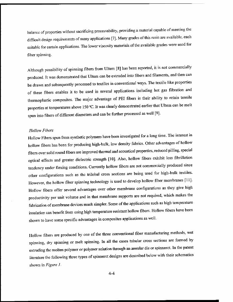
balance of properties without sacrificing processability, providing a material capable of meeting the
difficult design requirements of many applications [7]. Many grades of this resin are available, each
suitable for certain applications. The lower viscosity materials of the available grades were used for
fiber spinning.
Although possibility of spinning fibers from Ultem [8] has been reported, it is not commercially
produced. It was demonstrated that Ultem can be extruded into fibers and filaments, and then can
be drawn and subsequently processed to textiles in conventional ways. The textile like properties
of these fibers enables it to be used in several applications including hot gas filtration and
thermoplastic composites. The major advantage of PEI fibers is their ability to retain tensile
properties at temperatures above 150 «C. It was clearly demonstrated earlier that Ultem can be melt
spun into fibers of different diameters and can be further processed as well [9].
Hollow Fibers
Hollow Fibers spun from synthetic polymers have been investigated for a long time. The interest in
hollow fibers has been for producing high-bulk, low density fabrics. Other advantages of hollow
fibers over solid round fibers are improved thermal and acoustical properties, reduced pilling, special
optical effects and greater dielectric strength [10]. Also, hollow fibers exhibit less fibrillation
tendency under flexing conditions. Currently hollow fibers are not commercially produced since
other configurations such as the trilobal cross sections are being used for high-bulk textiles.
However, the hollow fiber spinning technology is used to develop hollow fiber membranes [11].
Hollow fibers offer several advantages over other membrane configurations as they give high
productivity per unit volume and in that membrane supports are not required, which makes the
fabrication of membrane devices much simpler. Some of the applications such as high temperature
insulation can benefit from using high temperature resistant hollow fibers. Hollow fibers have been
shown to have some specific advantages in composites applications as well.
Hollow fibers are produced by one of the three conventional fiber manufacturing methods, wet
spinning, dry spinning or melt spinning. In all the cases tubular cross sections are formed by
extruding the molten polymer or polymer solution through an annular die or spinneret. In the patent
literature the following three types of spinneret designs are described below with their schematics
shown in Figure 1.
4-4
1. This annular spinneret has a solid pin supported in the center of the circular orifice. The polymer
is extruded through the annulus. In this type of design, a gas forming additive is incorporated in the
polymer melt. The gas fills the core of the fiber as it emerges from the annulus thus preventing the
collapse of the fiber before it solidifies.
2. Another spinneret design has a hollow needle or tube supported in the center of the orifice and
an inert gas or liquid is injected through the needle to maintain the tubular shape until the
solidification or coagulation of the fiber.
3. A third type of hollow fiber spinneret has a C-shaped orifice with the tips of the C overlapping.
The polymer solution or melt welds into a tube after extrusion through the C-shaped die. The gas
required to keep the fiber hollow is drawn in through the gap in the extruded fiber upstream from
the weld point [12].
There has been some interest in hollow carbon fibers as it was shown that hollow carbon fibers had
higher tensile strength and modulus than that of general solid carbon fibers, which offer some
advantages in composite design [13]. Composites formed from hollow fibers showed higher
anisotropy in thermal conductivity measurements compared to that formed from solid carbon fibers
[14]. When the above mentioned methods were used to produce pitch based carbon fibers each
method showed its advantages and disadvantages. It was not possible to produce uniform hollow
fibers using the annular die with an insert in the center. Since mesophase pitch solidifies
immediately as it comes out of the spinneret, it was observed that with C-shaped dies high melt
temperatures and high draw down rates had to be used. Alternatively, a new capillary design
consisting of three arc-shaped channels is also being investigated [15]. It is clear that capillary
design suitable for one type of polymer is not necessarily effective for another system.
4-5
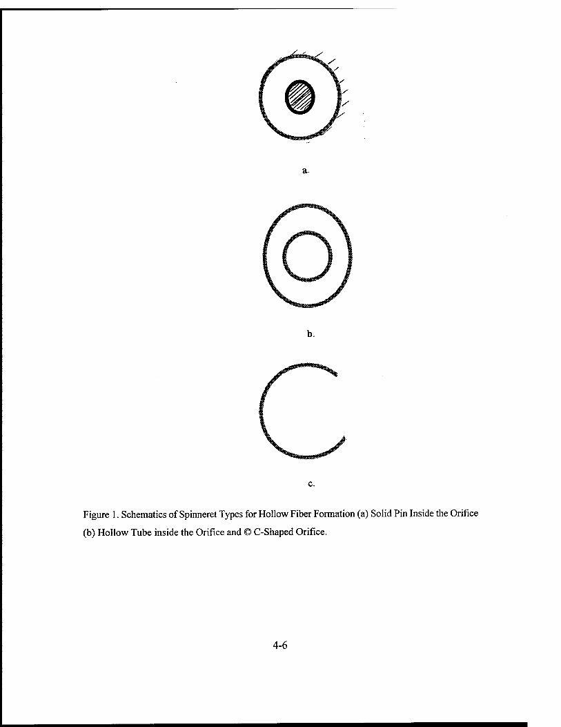
a.
Figure 1. Schematics of Spinneret Types for Hollow Fiber Formation (a) Solid Pin Inside the Orifice
(b) Hollow Tube inside the Orifice and © C-Shaped Orifice.
4-6

EXPERIMENTAL PROCEDURE
Materials
For this work, Ultem 1000 series (Ultem 1000 and 1010), which is the low viscosity grade polymer,
was selected since fiber spinning demands much lower viscosity compared to typical molding
processes. The properties of the polymer, including its viscosity behavior have been reported earlier
[9]. For solution processing, Methylene Chloride was used as a solvent. For the production of hollow
carbon fibers, AR mesophase pitch was used. Ultem polymers were dried in an oven at 150 °C for
at least four hours before processing.
Melt Spinning Set-Up
A special melt spinning unit was built for conversion of Ultem and other melt spinnable resins into
fibers of required properties. Unlike many other thermoplastic polymers that are typically spun into
fibers, such as nylons, polyesters, and polyolefins, Ultem or other high performance materials
demand much higher processing temperatures. The system should be capable of withstanding higher
temperatures for prolonged periods of time. Also, for hollow fiber formation, special arrangements
have to be made as described above. For this reason possibility of processing the polymer through
the use of a solvent was also explored.
The spinneret design with a hole-inside-hole type of arrangement was used for this research. Figures
2 and 3 show the schematic of the melt spinning apparatus. The key component is the capillary
design which consists of a hole inside the hole. This arrangement allows the polymer melt or
solution to come out through the annulus and flow of a fluid through the inner capillary torn
maintain the hollowness of the fiber till it solidifies. There was also an arrangement to change the
position of the inner capillary with respect to the annulus. By simply turning the knob, it is possible
to have the capillary in-line with the annulus, projecting below or lagging behind, depending on what
is desired, In the studies reported here, capillary was extending below the annulus by one mm. Other
features include, spinneret, filter, the thermocouple and air/vacuum connection. The whole system
when fully assembled, sits in a temperature controllable heating jacket.
4-7
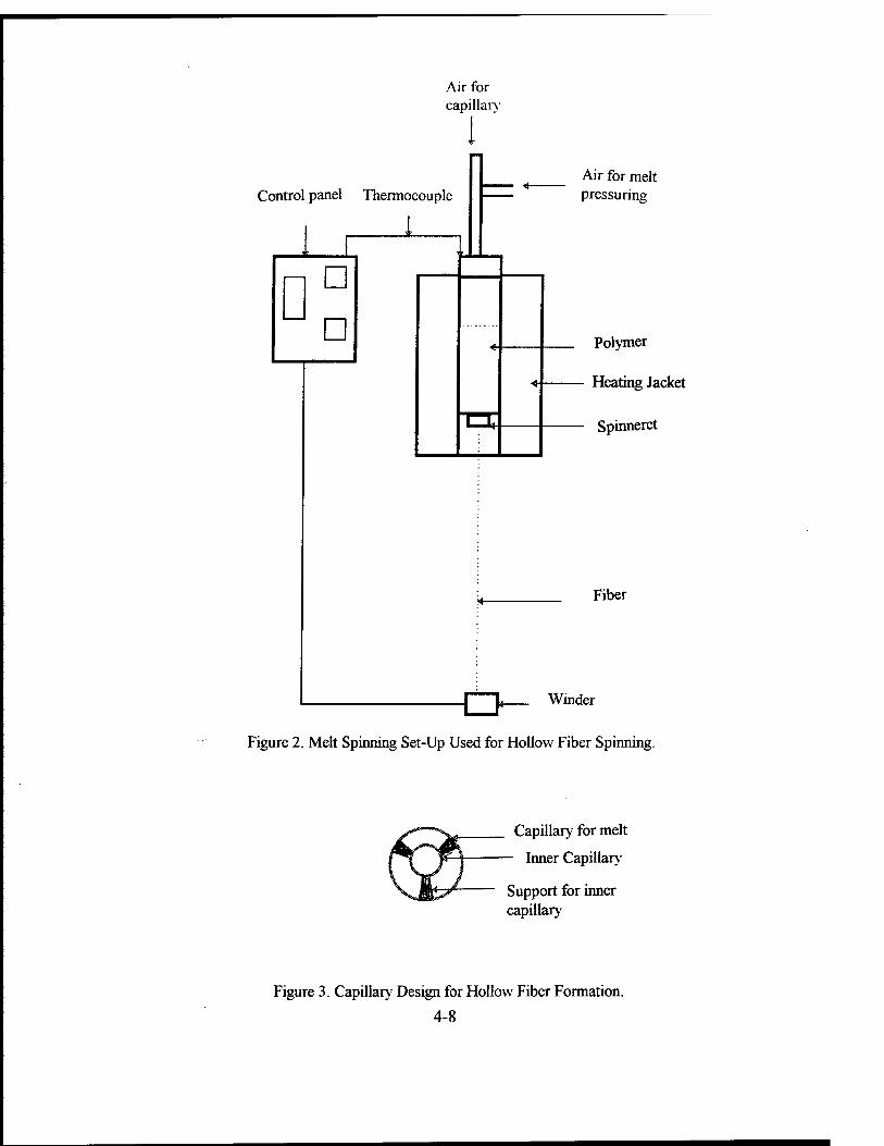
Air for capillary
i ' Control panel Thermocouple
1
l—Jk
Air for melt pressuring
Polymer
Heating Jacket
Spinneret
Fiber
o- Winder
Figure 2. Melt Spinning Set-Up Used for Hollow Fiber Spinning.
Capillary for melt
Inner Capillary-
Support for inner capillary
Figure 3. Capillary Design for Hollow Fiber Formation.
4-8

RESULTS AND DISCUSSION
Melt Spinning ofUltem
Melt spinning of the polymer was done using a home-built spinning unit described in the previous
section. The important variables in spinning are, melt temperature, melt pressure, quenching
conditions and winding speed. In this study, melt temperature, melt pressure, and winding speed
were varied. There was no positive feeding of the melt and thus the flow rate could not be positively
controlled, but was determined by melt temperature and pressure. Quenching was done by ambient
air with no special air flow attachments.
Although fibers were collected, spinning was not without any problems. Obviously the temperature
of the melt to achieve flow through the spinneret was very high. It is because of the very high
viscosity of the polymer, as the resin was not made for fiber spinning, but for molding applications.
Another problem was that of air bubbles coming with the melt. To overcome this problem, in later
trials, vacuum was used during melting. This helped the flow of bubble free melt at least for the
initial period. It appears that as the polymer melts, in the presence of vacuum, the melt in the bottom
part of the pot is void free and in the upper part there are still air bubbles. However, for the amount
of material to be spun, use of vacuum served the purpose.
SEM pictures of the material as it comes out of the spinneret and the hollow fibers spun at different
wind-up speeds are shown in Figures 4 and 5. It is evident from the pictures that the fibers are fairly
circular and have a large hole and a small annulus. The annulus is so small that it becomes difficult
to handle the fibers as can be seen from figure 5 which shows the tip coming together and appearing
as though it is not circular. All these fibers were spun with a very low flow rate of air in the inner
capillary. Figures 6 and 7 show the effect of too high an air flow or not having any air in the
capillary. Even a slight increase in the air flow through the capillary results in splitting of the fiber
and providing no air leads to collapsing of the polymer without a visible hole in the fiber, at least
in the processing conditions investigated. The mechanical properties and exact dimensions such as
fiber diameter, hollow ratio need to be characterized.
4-9
Figure 4. SEM Photograph of Hollow Fibers (immediately after extrusion).
4-10
Figure 5. SEM Photograph of Hollow Fiber (wound at 360 ft/min).
4-11
Figure 6. Photograph of Fiber spun With Higher Air Flow in the Capillary.
4-12
Figure 7. SEM Photograph of Fiber spun Without Air Flow in the Capillary.
4-13
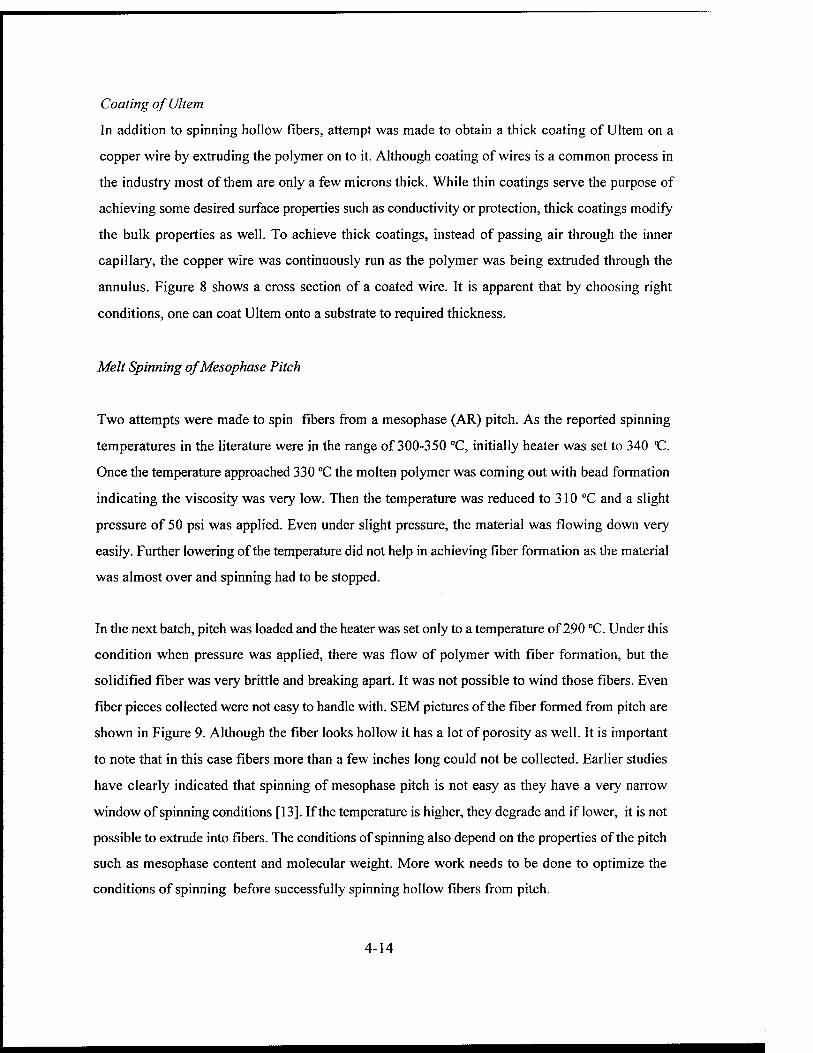
Coating of Ultem
In addition to spinning hollow fibers, attempt was made to obtain a thick coating of Ultem on a
copper wire by extruding the polymer on to it. Although coating of wires is a common process in
the industry most of them are only a few microns thick. While thin coatings serve the purpose of
achieving some desired surface properties such as conductivity or protection, thick coatings modify
the bulk properties as well. To achieve thick coatings, instead of passing air through the inner
capillary, the copper wire was continuously run as the polymer was being extruded through the
annulus. Figure 8 shows a cross section of a coated wire. It is apparent that by choosing right
conditions, one can coat Ultem onto a substrate to required thickness.
Melt Spinning of Mesophase Pitch
Two attempts were made to spin fibers from a mesophase (AR) pitch. As the reported spinning
temperatures in the literature were in the range of 300-350 °C, initially heater was set to 340 "C.
Once the temperature approached 330 °C the molten polymer was coming out with bead formation
indicating the viscosity was very low. Then the temperature was reduced to 310 CC and a slight
pressure of 50 psi was applied. Even under slight pressure, the material was flowing down very
easily. Further lowering of the temperature did not help in achieving fiber formation as the material
was almost over and spinning had to be stopped.
In the next batch, pitch was loaded and the heater was set only to a temperature of 290 °C. Under this
condition when pressure was applied, there was flow of polymer with fiber formation, but the
solidified fiber was very brittle and breaking apart. It was not possible to wind those fibers. Even
fiber pieces collected were not easy to handle with. SEM pictures of the fiber formed from pitch are
shown in Figure 9. Although the fiber looks hollow it has a lot of porosity as well. It is important
to note that in this case fibers more than a few inches long could not be collected. Earlier studies
have clearly indicated that spinning of mesophase pitch is not easy as they have a very narrow
window of spinning conditions [13]. If the temperature is higher, they degrade and if lower, it is not
possible to extrude into fibers. The conditions of spinning also depend on the properties of the pitch
such as mesophase content and molecular weight. More work needs to be done to optimize the
conditions of spinning before successfully spinning hollow fibers from pitch.
4-14
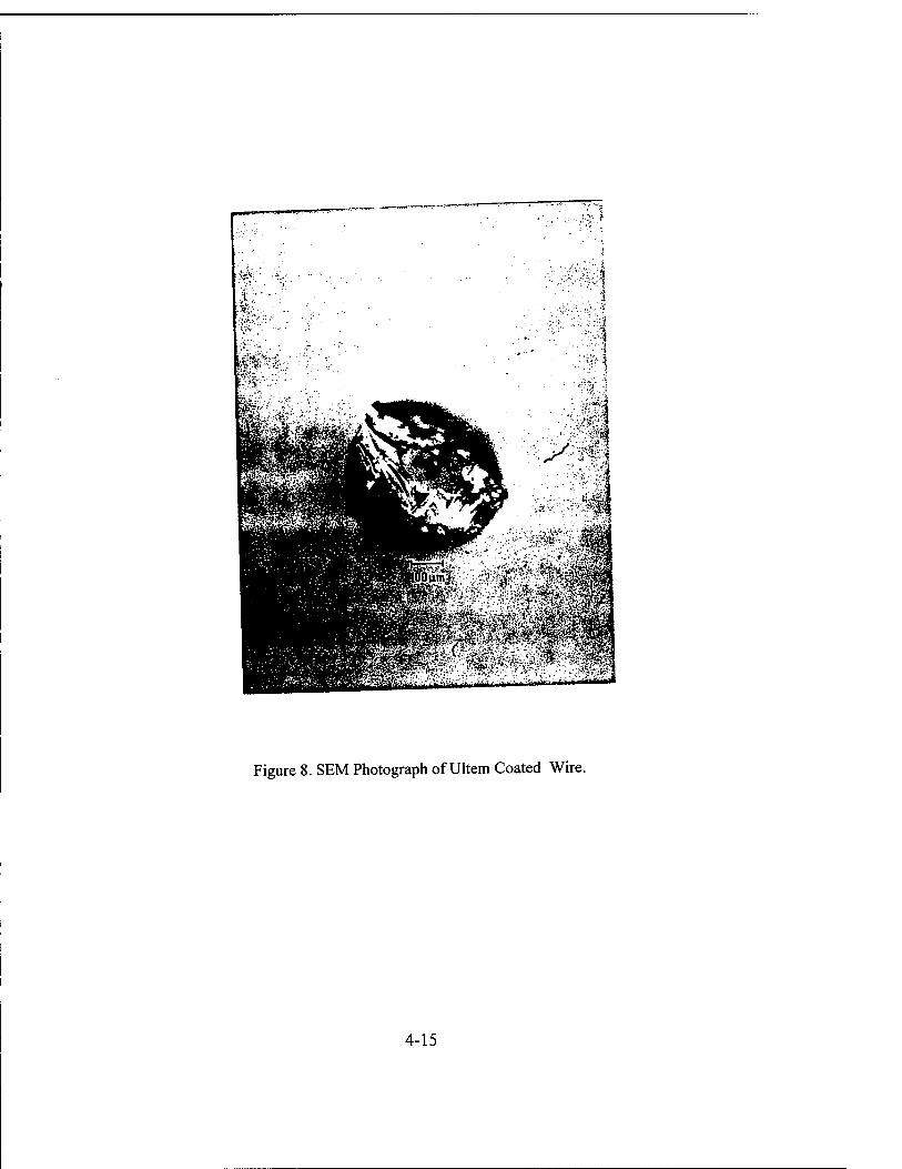
!..vy*
■^m
.... ^üfti^ww*
.1 ■in^iiitfff'iii"""' ,fi'"j>'-'
Figure 8. SEM Photograph of Ultem Coated Wire.
4-15
Figure 9. SEM Photographs of Melt Spun Pitch Fiber.
4-16
Solution Processing ofUltem
Since Ultem has a very high glass transition and softening temperatures melt processing is not easy.
In addition to the difficulties in working with higher temperatures, there is also going to be
degradation of the polymer under those conditions. As an alternative, solution processing of the
polymer with methylene chloride as solvent was explored. The main interest being to find out
whether viscous solutions of Ultem with high concentration of the polymer can be formed, and then
is it possible to obtain thick coating on copper wires using such a solution.
Solutions were prepared with different concentrations of Ultem in methylene chloride. It was easy
to dissolve upto 20 per cent (w/w). When the concentration was increased, it took longer to dissolve
the material. In fact the mixture had to be left overnight or slightly wanned to increase the
dissolution rate. Although viscosity of the dope was not checked, concentrations above 40 per cent
formed thick dope which appeared to be suitable for extrusion through a capillary such as for
spinning into fibers. Up to 50 per cent Ultem could be dissolved in methylene chloride solvent
without much difficulty leading to formation of a viscous dope. Although fibers were not spun,
copper wire was continuously passed through the spinneret achieving thick coating. Figure 10 shows
the cross section of a wire coated from Ultem solution. As there was no attempt made to center the
wire through the capillary, coating was not concentric. However, the results showed that solution
processing is quite promising.
RECOMMENDATIONS FOR FUTURE WORK
Although hollow fibers were spun from Ultem they were not thoroughly characterized. Fiber
structure and properties need to be characterized by microscopy, thermal analysis and tensile testing.
Possibility of spinning fibers from the solution need to be investigated. It should be possible to dry
spin the fiber. However care needs to be taken in designing the system so that evaporated solvent
can be recovered. Another aspect which needs detailed investigation is the spinning of hollow fibers
from mesophase pitch. Rheology of pitch, especially its viscosity change with temperature needs to
be characterized so that the exact range of processing temperatures can be determined. Based on that
data fibers can be spun from pitch. After that forming hollow fibers should be much easier.
4-17
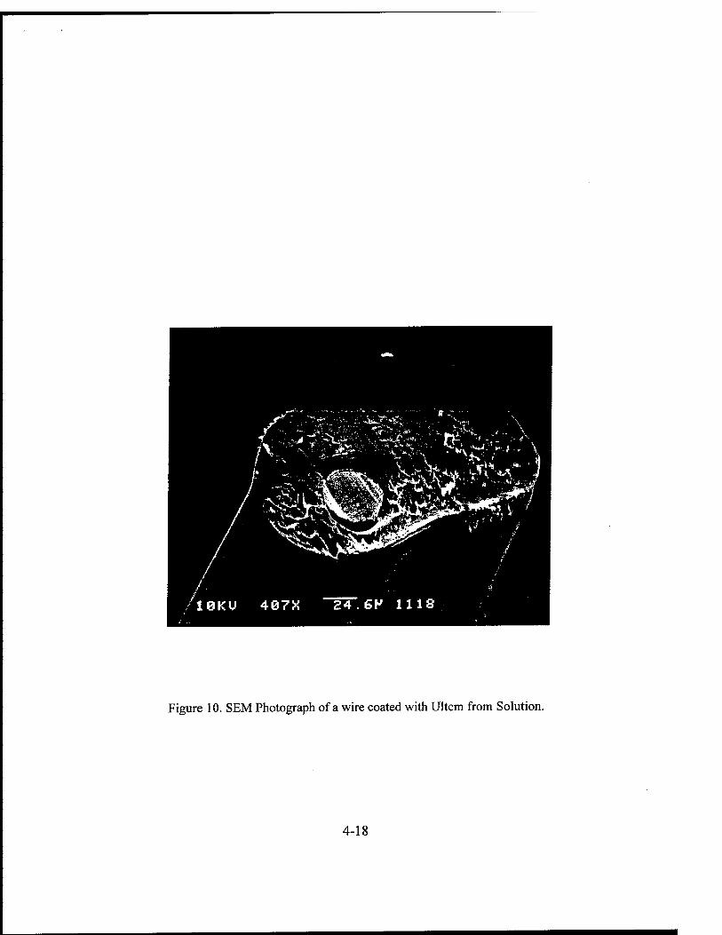
Figure 10. SEM Photograph of a wire coated with Ultem from Solution.
4-18

ACKNOWLEDGMENTS
Guidance and support from Drs. Phil Wapner and West Hoffman in this entire work is greatly
acknowledged. Colleagues at the laboratory, especially Drs. Jones, Pollock and Ismail and Miss
Marietta Fernadez, Hong Phan and Naomi are acknowledged for making my tour an enjoyable one.
Financial support from AFOSR, which made this work possible is greatly appreciated. Staff of RDL
for their cooperation is also acknowledged.
4-19

BIBLIOGRAPHY
1. H. H. yang, 'Aromatic high Strength Fibers,' John Wiley and Sons, New York (1989).
2. T. Kaneda, T. Katsura K. Nakagawa, H. Makino and M. Horio, J. Appl. Polym. Sei., 2,
32, 3133; 32, 3151 (1986).
3. P-84 High Performance Products, Company literature, Lenzing AG.
4. G. V. Cekis, Modern Plastics Encyclopedia, mid October issue, 32 (1993).
5. H. R. Penton, Modern Plastics Encyclopedia, mid October issue, 87 (1993).
6. Ultem Polyetherimide Resin, Company literature, GE Plastics.
7.1. W. Serfaty, in Polyimides, ed. by K. L. Mittel, Plenum Press, New York (1988).
8. "Textile Applications of Performance Polymers," Textile Month, July, 20 (1991).
9. G. S. Bhat, AFOSR Summer Project Report, 1995.
10. O. E. Brück, Textile Institute and Industries, 3, 118-121 (1965).
11. H. I. Mahon and B. J. Lipps, Encyclopedia of Polymer Science and Technology, Ed. H. F.
Mark pp258-272 (1984).
12. Reinehr et al, US Patent 4,457,885 (1984). 13. Y. Shi, Q. F. Zha and L. Liu, Proceedings of the European Carbon Conference "Carbon 96" -
New Castle, UK 226-227 (1996).
14. G. J. Hays et al., Carbon 1992 Extended Abstracts, Germany, 813-815 (1992).
15. Reinehr et al, US Patent 4,432,923 (1984).
4-20
BLACKHOLE ANALYSIS
David B. Choate Associate Professor
Department of Mathematics
Transylvania University 300 N. Broadway
Lexington, KY
Final Report for: Summer Research Program
Phillips Laboratory
Sponsored by: Air Force Office of Scientific Research
Boiling Air Force Base, Washington, DC
And
Phillips Laboratory
August, 1997
5-1
BLACKHOLE ANALYSIS
David B. Choate Associate Professor
Department of Mathematics Transylvania University
Abstract
Blackhole space is a parallel universe to the complex plane in which some problems can be
worked more easily and others with greater difficulty. The theorems of blackhole space are
presented here and their application to superposition in signal processing. Parallel programs exist
to any existing program, even some parallel machines.
5-2
BLACKHOLE ANALYSIS
1. BLACKHOLE ADDITION
Let S = {z = x + xj I x and y real, -7t < y < 7t} or equivalently, after an appropriate
adjustment of the residue of y modulo 2K, let S = {z = x + y (mod 2TC)J | X and y real}, a
horizontal strip. Set SB = S U {-<»}.
Now let z = xi + yJ and w = x2 + y?j e SB. Define a blackhole or B- multiplication on SB,
denoted by ©, as
z © w = (xi + x2) + [(yi + y2) mod (2TC)JJ
provided both z and w are in S; otherwise, z © w = -ao .
And if z = re"8, then as usual define Log(z) = ln|r| + [0 (mod 2TC)JJ again after the
appropriate adjustment of the residue. Clearly
Log(zw) = Log (z) © Log (w).
Now let z, w 8 SB. We define an operation called blackhole addition or B-addition on
SB, denoted by j-, as
z rw = Log(ez + ew).
If we define z r -QO = z = z r - oo for every z in SB, then r is an operation on SB.
And clearly
Log (z + w) = Log (z) r Log(w).
5-3
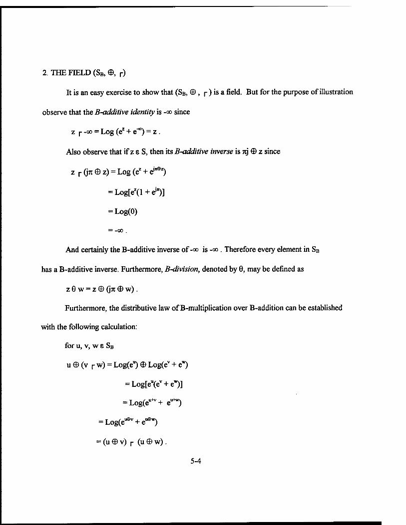
2. THE FIELD (SB, ©, r)
It is an easy exercise to show that (SB, ©, r )ls a fold- But f°r tne purpose of illustration
observe that the B-additive identity is -oo since
z r-oo = Log(ez + &") = z .
Also observe that if z 8 S, then its B-additive inverse is iq © z since
z r(J7t©z) = Log(ez + ej"ez)
= Log[ez(l+ei")]
= Log(0)
= -00
And certainly the B-additive inverse of-oo is -oo . Therefore every element in SB
has a B-additive inverse. Furthermore, B-division, denoted by 9, may be defined as
z9w = z©(jrc©w).
Furthermore, the distributive law of B-multiplication over B-addition can be established
with the following calculation:
for u, v, w e SB
u © (v r w) = Log(eu) © Log(ev + e*)
= Log[eu(ev + ew)]
= Log(eu+v+ eu+w)
= Log(euffiv + eu9w)
= (u © v) r (u © w) .
5-4
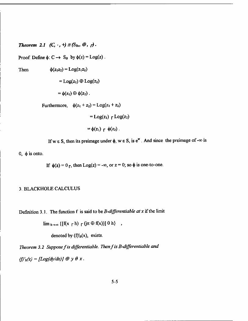
Theorem 2.1 (C, •, +) = (SB„ e, r).
Proof. Define (j>: C -> SB by <J>(z) = Log(z) .
Then <j>(ziz2) = Log(ziz2)
= Log(zi) © Log(z2)
= (t>(z!) © <t>(z2) •
Furthermore, <|)(zi + z2) = Log(zi + z2)
= Log(zi) rLog(z2)
= <t>(zi) r <t>(z2) •
If w 6 S, then its preimage under (j), w e S, is ew . And since the preimage of -oo is
0, (() is onto.
If <|>(z) = 0 r, then Log(z) = -oo, or z = 0; so <|) is one-to-one.
3. BLACKHOLE CALCULUS
Definition 3.1. The function f is said to be B-differentiable at x if the limit
limk_«,{[f(xrh)r(jw©f(x))]eh} ,
denoted by (O'BOO, exists.
Theorem 3.2 Suppose f is differentiable. Then f is B-differentiable and
(f)'B(x) = [Log(dy/dx)] eyBx.
5-5
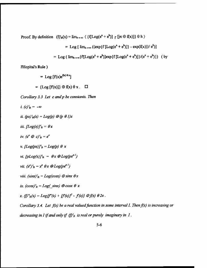
Proof. By definition (Q'B(X) = lim^ < {f[Log(ex + eh)] r \jn 0 f(x)]} 0 h >
= Log [ lim^ «exp{f [Log(ex + eh)]} - exp(f(x))>/ eh)]
= Log (linw{f[Log(ex + eh)]exp{f[Log(ex + eh)]}/(ex + eh)}) ( by
lHopital's Rule )
= Log[f(x)ef(x)ex]
= {Log[f(x)]}©f(x)0x. D
Corollary 3.3 Let c andp be constants. Then
i- (C)'B = -°°
ii. (px)'B(x) =Log(p) &(p 01)x
in. [Log(x)]'B = Ox
iv. (ex Q c)'B = ex
v. [Log(px)]'B = Log(p) 0 x
vi. fpLog(x)J'B = 0x GLogfryT1)
vii. (XTJ'B = X? OX &Log(pxr')
viii. (sinxj's - Log(cosx) (Bsinx Ox
ix. (COSXJ'B =Log(_sinx) (Bcosx 0 x
x. (f) \(x) = Log{f(x) + [f(x)f - f(x)} ef(x) 02x.
Corollary 3.4. Let f(x) be a real valued function in some interval I. Thenffx) is increasing or
decreasing in I ifand only if (f)'B is real or purely imaginary in I.
5-6
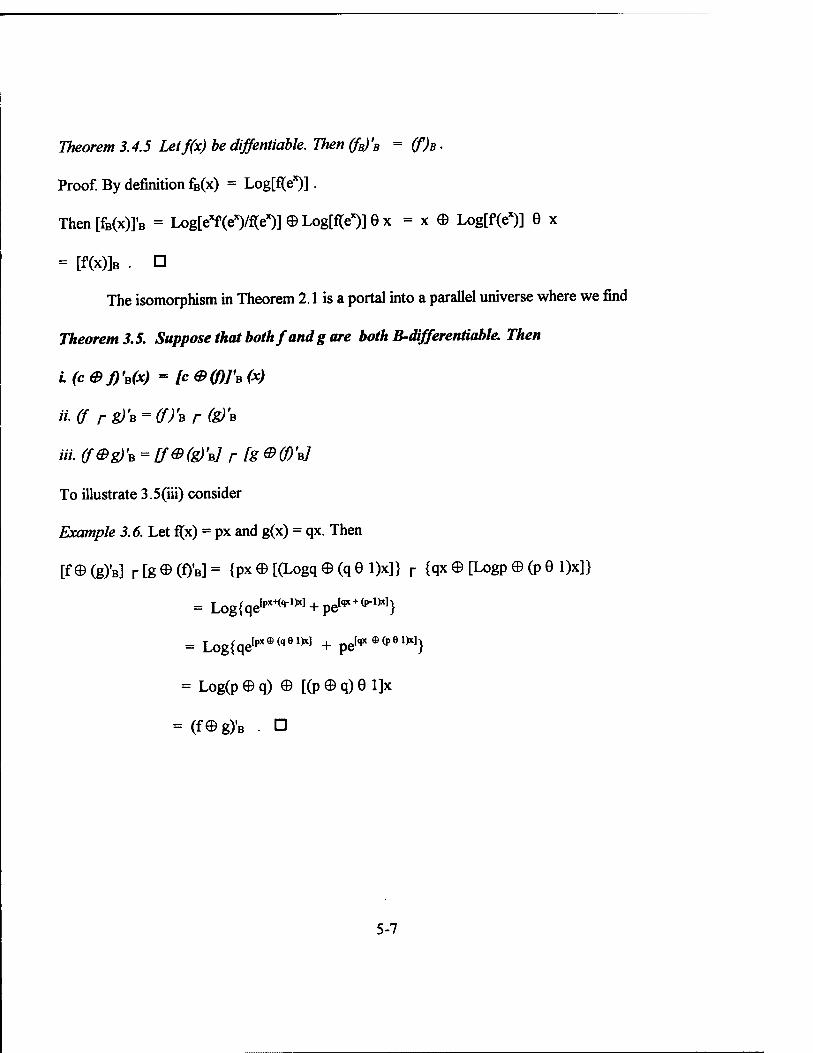
Theorem 3.4.5 Letf(x) be diffentiable. Then (fB)'B = (f)ß.
Proof. By definition fB(x) = Log[fi>x)].
Then [fB(x)]'B = Log[e*f(eW)]©Log[f(ex)]ex = x 0 Log[f(ex)] 9 x
= [f(x)]B . ü
The isomorphism in Theorem 2.1 is a portal into a parallel universe where we find
Theorem 3.5. Suppose that both fand gare both B-differentiable. Then
L(cef)'*(x) = [C&(0/'B(X)
n.(f rg)'* = (f)'*r(g)'*
m. (f&g)'B = [fG(g)V r fg ®0)'»J
To illustrate 3.5(iii) consider
Example 3.6. Let fix) = px and g(x) = qx. Then
[fe (g)'B] r [g © (O'BI = (PX © [(L°gq © (q e W) r (qx © [L°gp © (P
e W
= Log{qe[pxe(qei)x] + peI<pe(peiM}
= Log(p 0 q) 0 [(p 0 q) 6 l]x
= (f0g)'B . D
5-7
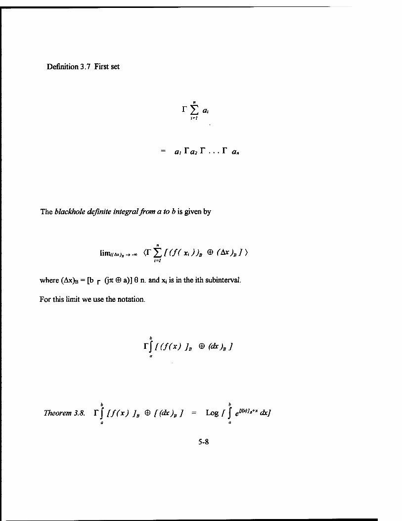
Definition 3.7 First set
FZ* i=l
ai To2 T . . . T a, n
The blackhole definite integral from a to bis given by
i=l
where (AX)B = [b p (J71 ® a)] Ö n ^d x> is i"tne fth subinterval.
For this limit we use the notation.
T\[(f(*)h ®(<b)B]
Theorem 3.8. TJ [f(x) ]B 0 [(dx)B ] = Log [ J emh+x dx]
5-8
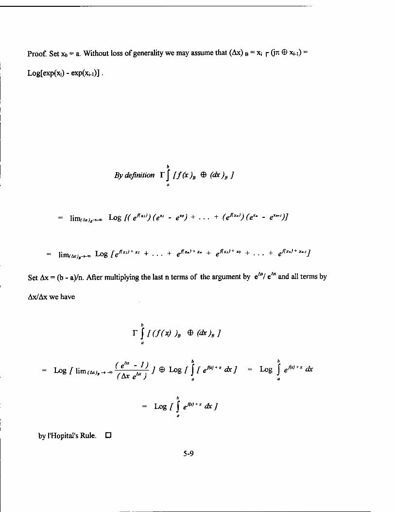
Proof. Set xo = a. Without loss of generality we may assume that (Ax) B = xj r (J7t © XM) =
Log[exp(xi) - exp(xj.i)].
By definition TJ [f(x)B 8 (dx)B ] a
= littVAx^-» Log f(eJ(x'))(ex' - e**) + • . . + (e**>) (e* - ex"')J
= lirrvAx^-» Log [e«x'> + xl + ... + eßxJ+x" + e«x,)+xo + ... + e***"*1]
Set Ax = (b - a)/n. After multiplying the last n terms of the argument by e*7 e^ and all terms by
Ax/Ax we have
T\[(f(x))B ®(dx)B] a
= Log [ lim^,-,~ (fK ~J! J®U>gf]f e^x dx] = Log J e«x)+x dx
b
= Log fj em + x dx] a
by lHopital's Rule. D
5-9
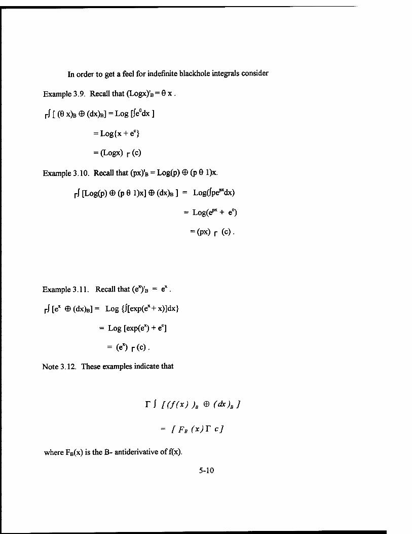
In order to get a feel for indefinite blackhole integrals consider
Example 3.9. Recall that (Logx)'B = 8 x .
rJ[(ex)B©(dx)B]=Log[Je0dx]
= Log{x + ec}
= (Logx) r (c)
Example 3.10. Recall that (px)'B = Log(p) © (p 9 l)x.
rJ [Log(p) © (p 0 l)x] © (dx)B ] = Logdpe^dx)
= LogCe1"1 + ec)
= (px) r (c) •
Example 3.11. Recall that (ex)'B = ex.
rJ [ex © (dx)ß] = Log {J[exp(ex+ x)]dx}
= Log [exp(ex) + ec]
= (ex)r(c).
Note 3.12. These examples indicate that
rJ [(f(x) )B ®(dx)B]
= [FB(x)T C]
where FB(x) is the B- antiderivative of f(x).
5-10
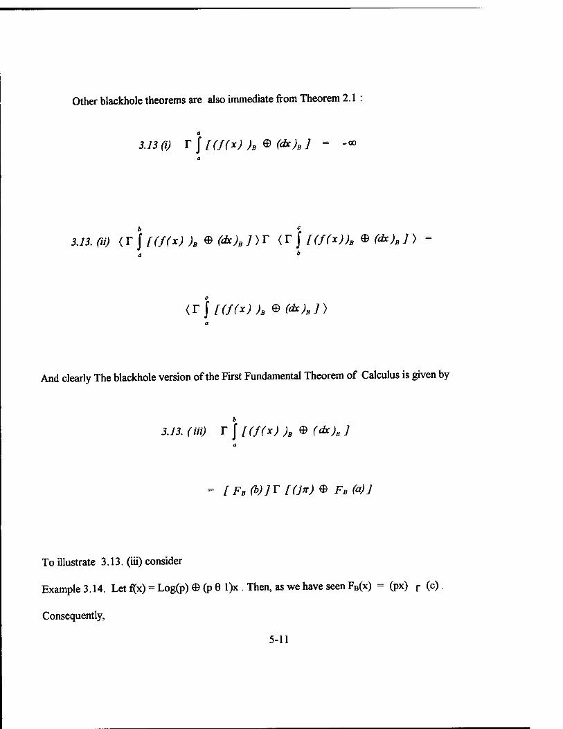
Other blackhole theorems are also immediate from Theorem 2.1
a
3.13 (i) T j f(f(x) )B 8 (dx)B 7 = -oo
3.13. (a) <r J [(f(x) )B®(dx)B])T <r f [(f(x))B e (<k)B j >
<rj/-r/r»;;a ©(*;,;>
And clearly The blackhole version of the First Fundamental Theorem of Calculus is given by
3.13. (in) r)[(f(x) )B @(dx)B]
= [ FBO>)]T [(j7t) 0 FB (a)]
To illustrate 3.13. (iii) consider
Example 3.14. Let f(x) = Log(p) 0 (p G l)x . Then, as we have seen FB(x) = (px) r (c)
Consequently,
5-11
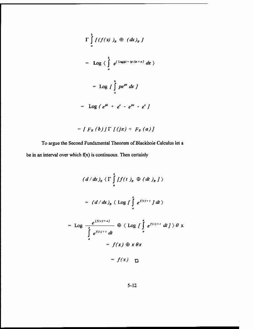
r J [(/(*) )B © (dx)B ] a
b
= Log < J jw»+w+*l ft) a
b
= Log [ j pe1" dx ] a
= Logfe*6 + ec - e1" - ecJ
= [F.(b)]T [(]*)+ F,(a)J
To argue the Second Fundamental Theorem of Blackhole Calculus let a
be in an interval over which f(x) is continuous. Then certainly
(d/cbe)B{T)[f(t)B ®(dt)B]) a
= (d/dx)B (Log [) ef(,)+,]dt)
Jf<*) + x] Log -^ © < Log / / ef(t) + t dt])e x
J ef(t, + t dt
f(x) © x Ox
= f(x) a
5-12

Now observe that
Theorem 3.16 (/£(x,y)dydx)B = Log(//exp{[f(x)JB+x+y}dydx).
Proof. (JJf(x,y)dydx) = {J[Jf(x,y)dy] dx} B B B
= (jLog<|exp{[n»] +y}dy>dx) B B
= (Logfexp<[exp{[f(x)] +y]dy>dx) B B
= Log<JJexp{[f(x)] +x + y}dydx>. D B
Example 3.17. Clearly (lnx + c )(lny + c ) = JJ(dx dy)/xy .
But observe that we can obtain this result through blackhole analysis. First descend to obtain
J/(l/xy) © (dx) © (dy) = 1/(9x9 y)©(dx) © (dy) B B B B B
= Log{JJ exp(-x - y + x + y)dxdy)
= Log[(x + Ci)(x + c2)
We now ascend to obtain
exp{Log[(lnx + c )(lny + c)]} = (lnx + c )0ny + c ). D 12 12
4. BLACKHOLE DIFFERENTIAL EQUATIONS
To understand how to apply blackhole calculus to ordinary space consider
Example 4.1 Let dy/dx = y
5-13
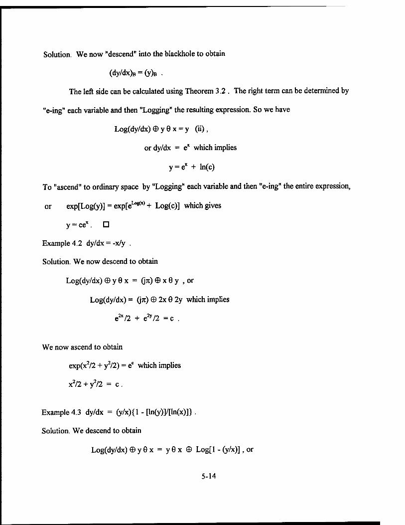
Solution. We now "descend" into the blackhole to obtain
(dy/dx>B = (y)ß .
The left side can be calculated using Theorem 3.2 . The right term can be determined by
"e-ing" each variable and then "Logging" the resulting expression. So we have
Log(dy/dx)©y0x = y (ii),
ordy/dx = ex which implies
y = ex + ln(c)
To "ascend" to ordinary space by "Logging" each variable and then "e-ing" the entire expression,
or exp[Log(y)] = expteF**0 + Log(c)] which gives
y = cex . D
Example 4.2 dy/dx = -x/y .
Solution. We now descend to obtain
Log(dy/dx) 0 y 0 x = Qn) © x 6 y , or
Log(dy/dx) = (JTt) © 2x G 2y which implies
e2*/! + e2*/! = c .
We now ascend to obtain
exp(x2/2 + y2/!) = ec which implies
x2/2 + ^12 = c.
Example 4.3 dy/dx = (y/x){l - [ln(y)]/[ln(x)]}.
Solution. We descend to obtain
Log(dy/dx) ©y9x = y0x© Log[l - (y/x)], or
5-14
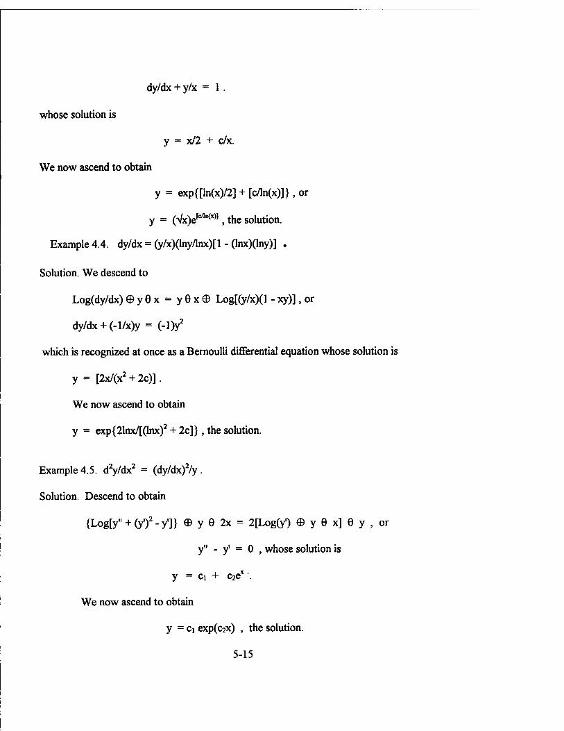
dy/dx + y/x = 1 .
whose solution is
y = x/2 + c/x.
We now ascend to obtain
y = exp{[ln(x)/2] + [c/ln(x)]}, or
y = (Vx)e[c/to(x)1, the solution.
Example 4.4. dy/dx = (y/x)(lny/lnx)[l - (lnx)(lny)] .
Solution. We descend to
Log(dy/dx)©y9x = y0xe Log[(y/x)(l -xy)], or
dy/dx+ (-l/x)y = (-Oy2
which is recognized at once as a Bernoulli differential equation whose solution is
y = [2x/(x2 + 2c)].
We now ascend to obtain
y = exp{21nx/[(lnx)2 + 2c]}, the solution.
Example 4.5. d2y/dx2 = (dy/dx)2/y .
Solution. Descend to obtain
{Log[y" + (y')2-y']} ® y 6 2x = 2[Log(y') © y 6 x] 9 y , or
y" - y' = 0 , whose solution is
y = Ci + c2ex".
We now ascend to obtain
y = Ci exp(c2x) , the solution.
5-15

5. BLACKHOLE SIGNAL PROCESSING
All undefined and underdefined terms and symbols used in this section can be found in
chapter 5 of [1]. In fact on p. 481 of [1] we are given a definition of a superposition H, a
generalization of a system transformation, which must satisfy:
1. H[Xl(n) D x2(n)] = H[x,(n) ° x2(n)]
2. H[c : x(n)] = c * H[x(n)].
, where D is an input operation and ° is an output operation and where
: and ♦ represent scalar multiplication.
Now define H: C -+ SB by H(z) = Log(z).
If we let i. D be +, ordinary addition in C,
ii. ° be r, or subaddition in SB ,
iii. : be scalar multiplication in C,
and iv. ♦ be a scalar operation in SB over C defined by
c * H[x]=Log(c)© H(x),
then we have a generalized superposition H (where H stands for homomorphism)
But by p.482 of [1] we can show that this homomorphic system can be written as a
cascade of three systems provided that p is commutative and associative
and that we can prove
Theorem 5.1. The additive group SB space under r is a vector space over C with scalar
multiplication 4*.
Proof. Let a,ß E C and v, w E SB . We can now easily establish the four properties of a vector
space.
5-16
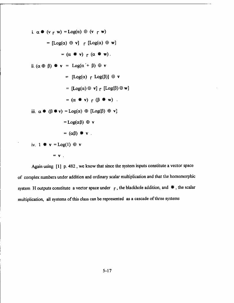
i. a* (v r w) =Log(a) 0 (v r w)
= [Log(a) 0 v] r [Log(a) 0 w]
= (a * v) r (a * w).
ü. (a e ß) * v = Log(a'+ ß) 0 v
= [Log(a) r Log(ß)] © v
= [Log(a)0 v] r [Log(ß)0w]
= (a * v) r 0 * w) .
iii. a* (ß*v) =Log(a) 0 [Log(ß) 0 v]
= Log(aß) 0 v
= (aß) * v .
iv. 1 * v =Log(l) 0 v
= v .
Again using [1] p. 482 , we know that since the system inputs constitute a vector space
of complex numbers under addition and ordinary scalar multiplication and that the homomorphic
system H outputs constitute a vector space under r, the blackhole addition, and *, the scalar
multiplication, all systems of this class can be represented as a cascade of three systems
5-17
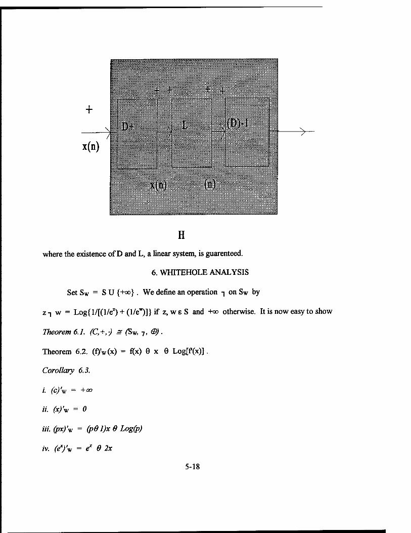
p i
+
x(n) ^
iffis
aüi iilliii
^
H IB
iV«V<V»«»w»i'iMViiimim>>>
lyjwwwiwwy
iHiiiiVriViYliVtYiViiV»WH»
(D)-I
******H**Humiimntttttn
x(a) (a)
j^S««a««s5»»
->
H
where the existence of D and L, a linear system, is guaranteed.
6. WHITEHOLE ANALYSIS
Set Sw = S U {+QO} . We define an operation T on Sw by
z-| w = Logll/^l/e^ + Cl/e*)]} if z, weS and +00 otherwise. It is now easy to show
Theorem 6.1. (C,+,-) = ßv, 7, &) .
Theorem 6.2. (f)'w(x) = f(x) 9 x 6 Log[f(x)].
Corollary 6.3.
i. (c)'w = +00
ii. (x)'w = 0
Hi. (px)'w = (pei)x 0 Log(p)
iv. (ex)'w = ex 0 2x
5-18

v. (-ex)'w = -ex
vi. fLog(px)J'w = [Log(x)J 0 x
vii. [pLog(x)]'v = [Log(x/p)] 0x
viii. [sin(x)]'w = sin(x) 0x6 Log[cos(x)]
ix. fpLog(x)J'w = cos(x) 0x0 Log[-sin(x)]
x. [f'Jw =y0 2x0 Log[(yf - y' -y"J.
Theorem 6.4. [Jf(x)dx]w = 0Log {0[jem*x1 dx J} .
Theorem 6.5. (y/s & (y)'w = 2(y 0 x) .
7. BLACKHOLE PROGRAMMING
We know, by Theorem 2.1, that every operation and function
has a unique blackhole image. For example
1. f(x) -»Logfte")] 2. d2y/dx2 -> {Log[(d2y/ox2) © (dy/dx)2 © dy/dx]} © y 0 2x
Consequently there exists a meta-blackhole algorithm which will accelerate any program
in which multiplication and exponentiation dominate addition and subtraction.
5-19

Reference
1. Oppenheim, A. V., and R. W. Schäfer: "Digital Signal Processing," Prentice-Hall, Inc, 1975.
5-20
IMAGE RECOVERY USING PHASE DIVERSITY
Neb Duric Professor
Department of Physics and Astronomy
University of New Mexico 800 Yale Bid. NE 87131
Final Report for: Summer Faculty Research Program
Phillips Laboratory
Sponsored by: Air Force Office of Scientific Research
Boiling Air Force Base, DC
And
Phillips Laboratory
October, 1997
6-1
IMAGE RECOVERY USING PHASE DIVERSITY
Neb Duric Professor
Department of Physics and Astronomy University of New Mexico
Abstract
The use of phase diversity to recover aberration-free images was the focal point of the research carried out under the Summer Faculty Research Program. Computer simulations were used to demonstrate that phase diversity can be used to remove aberrations from an image and that the Gonsalves error metric approach can be successfully implemented toward that goal. An experiment was designed to utilize a phase diversity camera for imaging aberrated wavefronts. It is proposed that such an experiment be carried out in order to determine the effectiveness of the phase diversity technique under "real life" conditions.
6-2
Image Recovery Using Phase Diversity
1 Introduction
The problem of imaging through the Earth's atmosphere can be addressed through a variety of well documented techniques. These techniques can be divided into "active" and "passive" categories. In the former, the optical elements of the imaging device (ie the camera) are adjusted in real time in order to counter the effects of the atmosphere as it varies spatially and temporally. In the latter case, no active components are used and the images are recovered through post-detection image processing.
The active method has the advantage that recording of faint signals can be achieved through integration of the signal on time scales much greater than the atmospheric coherence time. The Starfire Optical Range houses two active telescopes that operate this way. Stunning images approaching the diffraction limit have been recorded at SRO and represent the state-of- the art in active optics imaging through the Earth's atmosphere. The only drawback to this method is that it is technologically involved and therefore
expensive. The passive methods have met with more limited success. Their pri-
mary drawback is that post-detection processing requires a large number of pre-recorded images in order to time-resolve the coherence time of the atmo- sphere. Each recording of the image is therefore accompanied by detector noise. The combination of large numbers of image frames and noisy data make post-processing both difficult and time-consuming. The quality of the image cannot be assessed in real time. The major advantage, however, is that post-processing is inherently much cheaper than the construction of active optics and therefore presents greater availability to users.
The ideal passive technique, therefore, is one that minimizes the post- processing time and the detector noise limitations. One method that poten- tially bears such attributes is the Phase Diversity Technique. We report on the work we have performed, under the summer faculty program, relating to the phase diversity technique of image recovery. First, we describe the basic theoretical elements of this technique in the following section. Simulations we have performed are described in section 3. Section 4 describes an exper- imental setup for testing the phase diversity technique. Section 5 describes
6-3
future steps that need to be followed in order to recover images taken through the Earth's atmosphere.
2 Theoretical Basis of Phase Diversity
The Earth's atmosphere acts as an aberrator in which the aberrations vary spatially and temporally. For imaging objects at infinity one can consider the atmosphere as disturbing a wavefront which is initially plane-parallel, that is, surfaces of constant phases are planes oriented at right angles to the direction of propagation. As the plane wave travels through the Earth's atmosphere, different parts of the wavefront undergo different amounts of phase retardation resulting from the fact that different patches of the Earth's atmosphere have different indices of refraction. By the time the wavefront reaches the ground-based detector it is no longer plane-parallel. It has an overall tilt and the surfaces of constant phase are now corrugated. The corrugations represent phase variations (aberrations) imposed by the earth's atmosphere. For a wavefront incident on a circular aperture such as the aperture of a telescope, the aberrations can be expanded in a convenient series of functions called "Zernike Polynomials". Thus, any aberration can be, in principle, characterized by an appropriate set of Zernike polynomials. Any technique that can determine the coefficients of the Zernike polynomials can yield a characterization of the aberration and therefore can "undo" the aberration through an appropriate deconvolution.
The phase diversity technique takes advantage of the fact that the mor- phology of an image located at an arbitrary location with respect to the focal plane is a strong function of the aberrations that are present. Thus, the appearance of a defocused image, relative to an in-focus image, depends very much on the aberrations that the two images share. There are two basic methods by which the comparison of the defocused and focused images can be used to recover diffraction-limited images. We discuss them in'turn.
2.1 The Gonsalves Error Metric
The passage of the wavefront through the atmosphere and the optical system of the instrument leads to distortions of the true wavefront and therefore the image that is recorded by the instrument. The relationship between the
6-4
true image (as would be obtained by a diffraction limited instrument in the absence of the atmosphere) and the recorded image is given by:
r(x,y) = I(x,y)*((x,y) (1) where, I'{x,y), is the recorded image, I(x,y) is the true, diffraction-limited (aberration-free) image and ({x,y) is the point-spread function of the com- plete optical system (atmosphere plus instrument). The point spread func- tion is defined by the aberrations present in the optical system.
Taking the Fourier transform of both sides of equation 1 yields
I'(u,v) = I(u,v)C(u,v)
where ((u,v) is commonly referred to as the Optical Transfer Function or OTF.
Consider now a second image that is produced by the same instrument at the same time. This image is defocused with respect to the first. Thus,
I'd{u, v) = Id(u, v)(d(u, v). (2)
One can define an "error" as:
E = £ | J'(u, v) - /(«, v)C(u, V)\2 + Y: |5(«, V) - Id(u, «)&(«, v)\2 (3)
u,v u,v
where the summation is over the pixels of the digitized image. This error arises from not knowing the exact form of the OTF, £(ti, v). The goal, there- fore, is to minimize E by choosing the appropriate OTF. The modeling of the OTF is performed by: (i)assuming ((u,u) can be described by a series of Zernike polynomials, (ii)satisfying the additional constraint that the defocused term of the error equation must be simultaneously minimized.
Differentiating equation 3 with respect to /, setting to 0, solving for / and plugging back into equation 3 yields,
l/'(u, v)Uu, v)\2 - I>d(u, tQC(n, ^)|2 (4)
tr ic(«,w)ia + ic<(«,«)ia
Further minimization of the above error equation can be achieved by choosing the appropriate OTF. The usual approach is to expand the OTF in terms of Zernike Polynomials and by varying the polynomial coefficients, minimize E. The method was first proposed by Gonsalves (1979, 1982).
6-5
d V2 \ I — + + k A, dz 2k l
2.2 The Transport Method
This technique is based on a description of the transport of light through the focal plane along the optical axis of the instrument (henceforth the z axis). Let us consider the amplitude and phase of the wavefront.
V = Aeiwi = VleiSeiwt (5)
where V is the instantaneous electric field, / is the intensity, u is the fre- quency (we are assuming monochromatic radiation) and 8 is that portion of the phase of the signal that is produced by the aberrations.
The transport of the amplitude and phase along the z axis is normally described with the Helmholtz equation. If we assume that the wavefront can be described as a plane wave traveling in the z direction and if it's amplitude varies slowly with z, the transport equation simplifies to
0. (6)
where k is the wave number. Substituting equation 5 into equation 6 yields:
Equation 7 can be solved by numerical techniques such as the finite difference method. In general, 8 is a function of x and y, coordinates that define a plane perpendicular to the z axis. A solution of equation 7 for 6(x,y) can be expressed in terms of Zernike polynomials and can therefore be used to correct the aberrations represented by the OTF. This method is described by Restaino (1992).
3 Simulations
To test the feasibility of the above ideas, we have performed numerical simu- lations. The simulations were performed under the summer faculty program during the summer of 1997. The Gonsalves error metric approach was imple- mented numerically by modifying a code originally written by Gordon Love (PL). A known image (the true image) was numerically convolved with a point spread function simulated by a finite series of Zernike terms, yielding the aberrated image.
6-6
A defocused image was also generated by numerically smoothing the aber- rated image by a fixed amount of defocus, yielding the defocused image. Fig- ure 1 shows the true image, the aberrated image and the defocused aberrated image, respectively.
The simulated images were manipulated in the IDL environment using both in-house programs and IDL programs. A test image was recorded onto a CCD camera by shining light through small apertures arranged in an ap- proximate triplet pattern (figure la). This test image represents the "true" image, I(x,y) introduced earlier. The image was degraded by numerically applying a phase screen described by the first seven terms of the Zernike ex- pansion (figure lb), yielding I'(x,y). The defocused image, I'd, was aberrated the same way but with an additional defocus term of 1 wave (figure lc).
A program was applied to find the local minimum from equation 3. The resulting relationship between I(u,v) and ((u,v) is given by,
j = IC + h~Q ICI2 + l6l2'
The above / represents the minimum error for a given OTF. An initial guess of the OTF is used to begin the process of further min-
imization. This is achieved by setting the terms of the Zernike polynomial expansion of ((u,v) and finding the resulting E. The method of steepest descent was then used to find the combination of coefficients that yielded the minimum E. The resulting C(u,v) represents the recovered OTF.
With the recovered OTF and recorded image, I'(x, y), in hand, the "true" image, I(x,y) was recovered through a deconvolution (using equation 1). The recovered image is shown in figure Id. Note that the true image and the recovered image are indistinguishable from each other.
The main purpose of the simulation was to demonstrate that phase diver- sity works in principle. In recovering the image we have also demonstrated the robustness of the image recovery software and shown it to be accurate. What the simulation cannot tell us is how well this method works in practise. Finite detector noise and the time-varying aberrations of the atmosphere are two factors which cause deviations from the ideal case represented by the simulations. We therefore put together a laboratory experiment to test the feasibility of the phase diversity technique under "real-life" conditions.
6-7
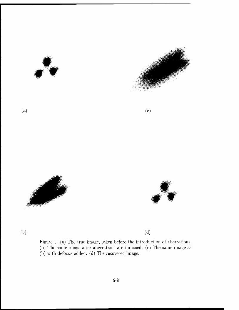
(a) (c)
(b) (d)
Figure 1: (a) The true image, taken before the introduction of aberrations, (b) The same image after aberrations are imposed, (c) The same image as (b) with defocus added, (d) The recovered image.
6-8
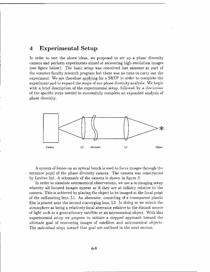
4 Experimental Setup
In order to test the above ideas, we proposed to set up a phase diversity camera and perform experiments aimed at recovering high-resolution images (see figure below). The basic setup was conceived last summer as part of the summer faculty research program but there was no time to carry out the experiment. We are therefore applying for a SREP in order to complete the experiment and to expand the scope of our phase diversity analysis. We begin with a brief description of the experimental setup, followed by a discussion of the specific steps needed to successfully complete an expanded analysis of phase diversity.
Camera L2 Aberrator LI Object
A system of lenses on an optical bench is used to focus images through the entrance pupil of the phase diversity camera. The camera was constructed by Lexitec Inc. A schematic of the camera is shown in figure 2.
In order to simulate astronomical observations, we use a re-imaging setup whereby all focused images appear as if they are at infinity relative to the camera. This is achieved by placing the object to be imaged at the focal point of the collimating lens, LI. An aberrator, consisting of a transparent plastic film is placed near the second converging lens, L2. In doing so we mimic the atmosphere as being a relatively local aberrator relative to the distant source of light such as a geostationary satellite or an astronomical object. With this experimental setup we propose to initiate a stepped approach toward the ultimate goal of recovering images of satellites and astronomical objects. The individual steps toward that goal are outlined in the next section.
6-9
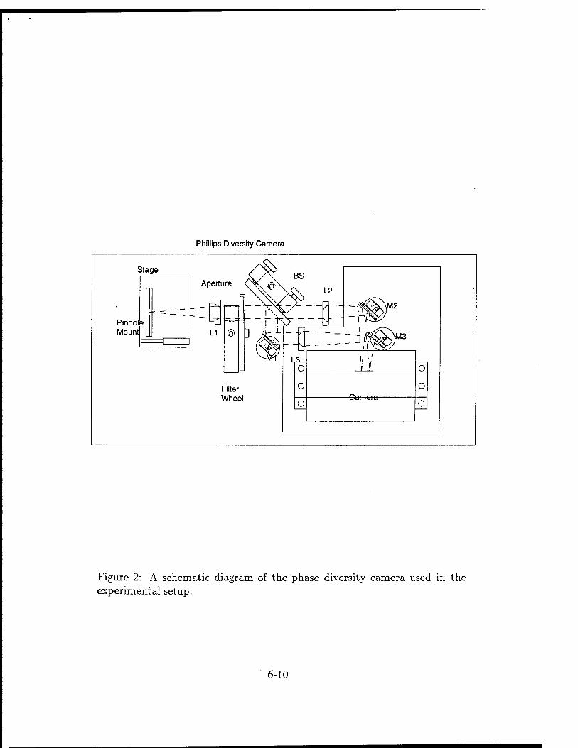
Phillips Diversity Camera
Stage
Pinhol Mount
Aperture
L1
L2
Filter Wheel
h-t-l^ ,M2
I
O
O
,M3
Camera
O
O
o
Figure 2: A schematic diagram of the phase diversity camera used in the experimental setup.
6-10
5 Future Work
5.1 Stationary Aberrations
The first element of a future, expanded analysis will be the implementation of the above experimental setup. The use of stationary aberrators will be used to determine the effectiveness of the phase diversity technique in recovering images of known morphology. This will be achieved through the experimental setup shown above, where collimated light from a known image will be passed through an aberrator before being focused onto the phase diversity camera. The recorded focused and defocused images contain phase errors imposed by the aberrator, which can be considered as a stationary phase screen. By varying the light level of the received signal and by varying the spectrum of aberrations the limitations of the phase diversity method can be explored.
5.2 Time Varying Aberrations
If, as the simulations suggest, the phase diversity technique proves successful in removing static aberrations from an image, the next step is to introduce time-varying aberrations into the imaging system to better replicate the tur- bulent nature of the earth's atmosphere. The atmosphere can also be thought of as a phase screen but one which changes its character on time scales of T0 ~ 1 — 100 ms. The phase diversity technique is therefore expected to work on images recorded over time scales shorter than the coherence time of the atmosphere. Time varying aberrations can be produced in the lab by using rotating pieces of aberrated glass or by generating turbulent motion of air with a localized heat source. The ultimate success of the image recovery will depend on two competing effects, the integration time, r, used to record the signal, and the coherence time, To, of the aberrations. The former builds up the signal to levels needed for the phase diversity technique to operate optimally. The integration time is a critical parameter in observations of faint sources such as earth-orbit satellites and distant astronomical objects. Under those conditions, even observations with ideal noise-free detectors are subject to photon-statistical noise (referred to as shot noise or Poisson noise). Thus, it is desirable to use as large a T as possible, in situations where the light level is low but at the same time, T < T0 is the necessary requirement for optimal use of the phase diversity technique. For r ~> r0, the phase diversity
6-11
technique fails. There is therefore a grey area, defined by r « r0, where the phase diversity technique does not work optimally but may nevertheless provide significant corrections to the aberrations. It is therefore necessary to fully explore and document this regime because of its relevance to image recovery at low light levels.
5.3 Comparison of Post-Processing Techniques
In order to test the post-processing element of the phase diversity technique it is necessary to recover images using both the Gonsalves Error Metric ap- proach (described in section 2.1) as well as the Transport approach (described in section 2.2). By using the two techniques under identical experimental conditions it is possible to compare them and determine their relative ro- bustness.
5.4 Celestial Observations
Once the phase diversity technique is fully explored in the lab, observations of celestial objects can be undertaken. At the low light levels afforded by such objects it will be necessary to access a research-class astronomical telescope. The PI has access to a 0.61 meter telescope at the Capilla Peak Observatory. This observatory is operated by the University of New Mexico and is located at a dark high-altitude site, 9300 feet above sea level. Our long-term goal is to attach the phase diversity camera to the telescope and repeat the above analyses, this time with the Earth's atmosphere as the aberrator.
6-12
6 References
Gonsalves, R.A. and Childlow, R. 1979, SPIE, 207, 32. Gonsalves, R.A. 1982, Optical Engineering, 829, 21. Restaino, S. 1992, Appl. Opt. 31, 7442.
6-13
THEORY OF PROTONS IN BURIED OXIDES
A. H. Edwards Associate Professor
Department of Electrical Engineering
University of North Carolina at Charlotte Charlotte, NC 28223
Final Report for: Summer Research Program
Phillips Laboratory
Sponsored by: Air Force Office of Scientific Research
Boiling Air Force Base, Washington, DC
And
Phillips Laboratory
August, 1997
7-1
THEORY OF PROTONS IN BURIED OXIDES
Arthur H. Edwards Associate Professor
university of North Carolina at Charlotte
Department of Electrical Engineering
Abstract
We have developed a model for electron capture at protons in a-S102 under U-V illumination. The
electrons are excited from the valence band to the gap level of the proton. The previously observed
temperature dependence can result from competition between hydrogen motion away from the defect
site and radiative recombination that would leave the proton as it was. At low temperature we argue
that the latter dominates. At elevated temperatures, the system is vibrationally excited which leads
to greater probability of hydrogen motion. This model not only explains previous observations,
it predicts new results that can be readily tested experimentally. This model is buttressed by ab
initio molecular orbital calculations and by a finite element analysis of vibraticnal spectra. Usin*
the vibraticnal wave functions, we have completed a vibronic model for electron capture, including
calculation of vibrational probability factors. This model is a work in progress. In an accompanying
proposal we discuss our plans for completion of this work.
7-2
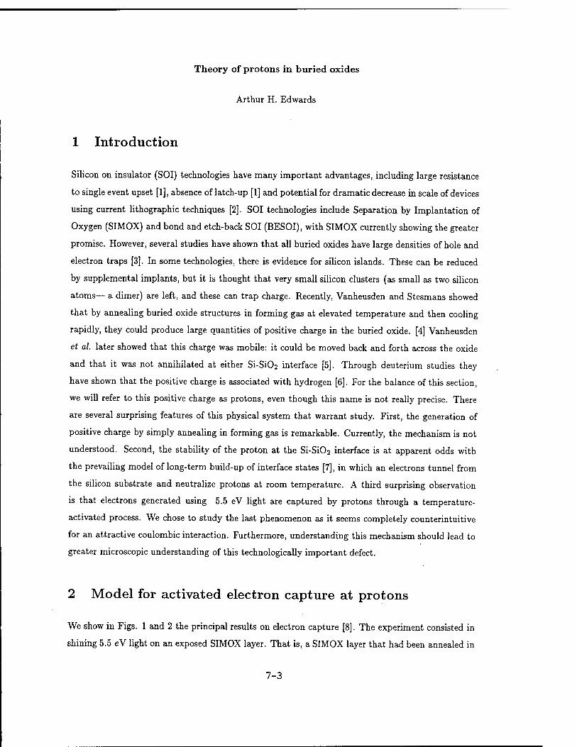
Theory of protons in buried oxides
Arthur H. Edwards
1 Introduction
Silicon on insulator (SOI) technologies have many important advantages, including large resistance
to single event upset [1], absence of latch-up [1] and potential for dramatic decrease in scale of devices
using current lithographic techniques [2]. SOI technologies include Separation by Implantation of
Oxygen (SIMOX) and bond and etch-back SOI (BESOI), with SIMOX currently showing the greater
promise. However, several studies have shown that all buried oxides have large densities of hole and
electron traps [3]. In some technologies, there is evidence for silicon islands. These can be reduced
by supplemental implants, but it is thought that very small silicon clusters (as small as two silicon
atoms— a dimer) are left, and these can trap charge. Recently, Vanheusden and Stesmans showed
that by annealing buried oxide structures in forming gas at elevated temperature and then cooling
rapidly, they could produce large quantities of positive charge in the buried oxide. [4] Vanheusden
et al. later showed that this charge was mobile: it could be moved back and forth across the oxide
and that it was not annihilated at either Si-Si02 interface [5]. Through deuterium studies they
have shown that the positive charge is associated with hydrogen [6]. For the balance of this section,
we will refer to this positive charge as protons, even though this name is not really precise. There
are several surprising features of this physical system that warrant study. First, the generation of
positive charge by simply annealing in forming gas is remarkable. Currently, the mechanism is not
understood. Second, the stability of the proton at the Si-Si02 interface is at apparent odds with
the prevailing model of long-term build-up of interface states [7], in which an electrons tunnel from
the silicon substrate and neutralize protons at room temperature. A third surprising observation
is that electrons generated using 5.5 eV light are captured by protons through a temperature-
activated process. We chose to study the last phenomenon as it seems completely counterintuitive
for an attractive coulombic interaction. Furthermore, understanding this mechanism should lead to
greater microscopic understanding of this technologically important defect.
2 Model for activated electron capture at protons
We show in Figs. 1 and 2 the principal results on electron capture [8]. The experiment consisted in
shining 5.5 eV light on an exposed SIMOX layer. That is, a SIMOX layer that had been annealed in
7-3
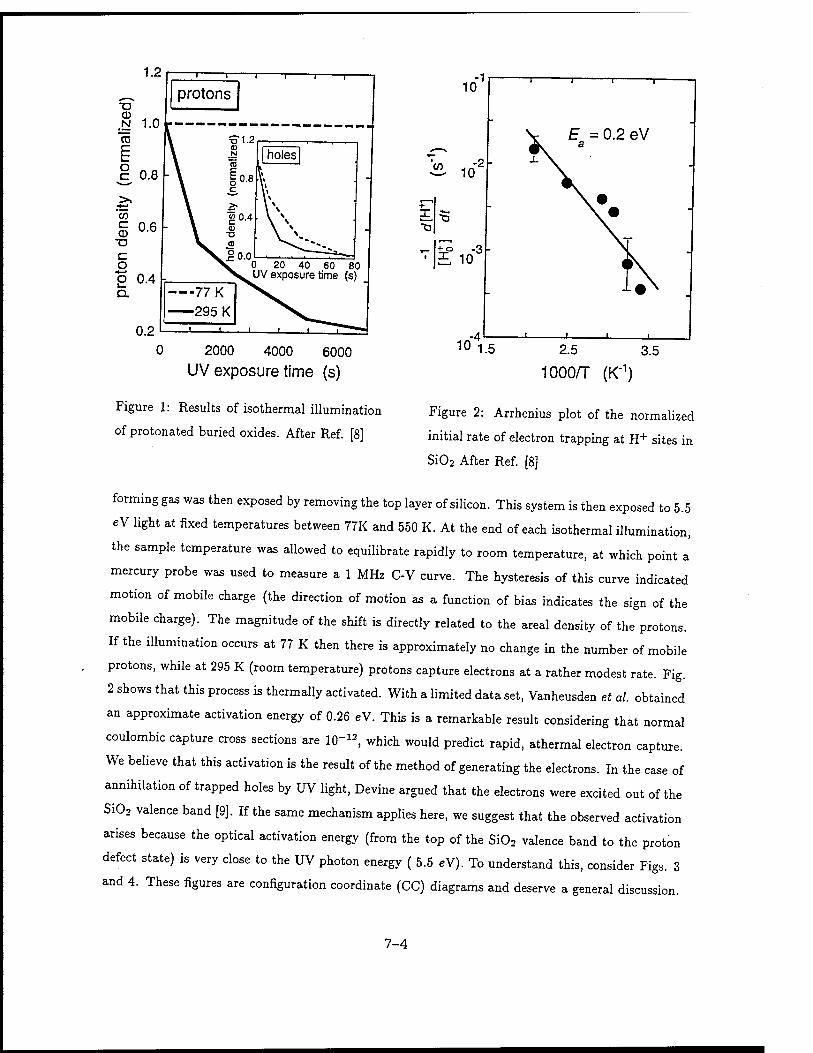
0 2000 4000 6000
UV exposure time (s)
Figure 1: Results of isothermal illumination
of protonated buried oxides. After Ref. [8]
10 1.5 2.5 3.5
1000/T (HC1)
Figure 2: Arrhenius plot of the normalized
initial rate of electron trapping at H+ sites in
Si02 After Ref. [8]
forming gas was then exposed by removing the top layer of silicon. This system is then exposed to 5.5
eV light at fixed temperatures between 77K and 550 K. At the end of each isothermal illumination,
the sample temperature was allowed to equilibrate rapidly to room temperature, at which point a
mercury probe was used to measure a 1 MHz C-V curve. The hysteresis of this curve indicated
motion of mobile charge (the direction of motion as a function of bias indicates the sign of the
mobile charge). The magnitude of the shift is directly related to the areal density of the protons.
If the illumination occurs at 77 K then there is approximately no change in the number of mobile
protons, while at 295 K (room temperature) protons capture electrons at a rather modest rate. Fig.
2 shows that this process is thermally activated. With a limited data set, Vanheusden et al. obtained
an approximate activation energy of 0.26 eV. This is a remarkable result considering that normal
coulombic capture cross sections are 10"12, which would predict rapid, athermal electron capture.
We believe that this activation is the result of the method of generating the electrons. In the case of
annihilation of trapped holes by UV light, Devine argued that the electrons were excited out of the
Si02 valence band [9]. If the same mechanism applies here, we suggest that the observed activation
arises because the optical activation energy (from the top of the Si02 valence band to the proton
defect state) is very close to the UV photon energy ( 5.5 eV). To understand this, consider Figs. 3
and 4. These figures are configuration coordinate (CC) diagrams and deserve a general discussion.
7-4
The Hamiltonian for a many atom system (either a molecule or a solid) can be written
Htot = Hel + Hlatt + Hel^latt (1)
where
H^= £ 2ÄTV« (2) a=l ZMa
Hel + Hel-latt = f;^-vl- T -4^4+ i £ ,1^ (3) fer2m« s \R*-fi\ 2atfeii^-^i
Here, Greek subscripts refer to nuclear coordinates, Roman refer to electronic coordinates, ne is
the number of electrons, Natoms is the number of atoms, {Ra} is the set of all nuclear coordinates,
and {fi} is the set of all electronic coordinates. It is customary to consider Hei + Hei^iatt to be the
electronic Hamiltonian, He. The total system wave function is assumed to have the form
%ct({rl},{Ra}) = x({Rc,})rK{fl}:{Rc}) (4)
where i>({fi}: {Ra}) is the wave function describing the electronic system, and is an eigenstate of
HeiP({r~i}:{Ra}) = EtrtdReWafi} :{Ra}). (5)
The colon indicates that the set of nuclear coordinates, {Ra}, is held fixed to calculate i>({fl}: {Ra}).
Etot{{Ra}) is usually called the total energy of the system. This is only true in a semiclassical picture
where the electrons are treated quantum mechanically and the lattice is treated classically. In the
full Born-Oppenheimer theory, where the lattice is also treated quantum mechanically, x{{R<*}) is
the wave function describing the nuclear or network motion and is an eigen state of of the following
Schrödinger equation
[Hiatt + Etot({Ra})]x{{Ra}) = EvibronicX{{Ra}) (6)
Now, Evibronic is the true total energy. Note that Etot({Ra}) now acts as a potential energy for
x{{Ra})- To calculate dipole matrix elements, we must evaluate
< Xi1>i\r\X/1>/ >=< Xi\Xf >< 4>i\r[1>f > (7)
so that the overlap of vibrational wave functions will be as important as the electronic matrix element
in determining the strength of an optical transition. This, of course, is the origin of Frank-Condon
transitions.
7-5
In applying B-0 theory, one usually simplifies dramatically the potential surface considered. In
the problem at hand we consider only the motion of the central hydrogen. As we will show below, this
is a reasonable assumption for the current system. Furthermore, we consider only one vibrational
mode at a time allowing us to draw one-dimensional potential surfaces. The pertinent CC would be
the stretch mode along the central OH bond direction. When multiple potential surfaces appear on
the same CC diagram, we must be careful that each represents the system with the same number of
electrons. The bottom curve in both figures 3 and 4 corresponds to a full valence band, an empty
conduction band and a hole on the OH group. In short, the ground state of the system with one
proton. The top curve corresponds to a hole in the valence band, an electron in the conduction band
and a hole on the OH group. The vertical distance between the bottom and top curves must be the
Si02 band gap. The middle curve corresponds to a hole in the valence band, an empty conduction
band and a neutral OH group. Note that this is a repulsive potential curve. Thus, the bottom and
top curves will give rise to true vibrational states, while the center curve will give vibrational wave
functions that are free-particle-like. Furthermore, the energy spectrum along the center curve will
be continuous.
In the first case, shown in Fig. 3, the photon energy is just below the Frank-Condon transition
energy. At low temperatures, only the ground vibrational state is occupied, so the transition prob-
ability will be very small (small | < Xi\Xf > |2)- At elevated temperatures, the excited vibrational
states will be occupied. The most obvious effect is that the optical transition energy is smaller by
a vibrational quantum, hu. What may be more important is that excited vibrational states have
maxima closer to the classical turning points. This can alter transition probabilities by altering
< Xi\Xf > so that transitions to states lower and higher on the center potential surface are stronger.
Because of the slope of this potential surface, the small change in energy (AE = hu) for the initial
state can lead to a large decrease in energy of the final state, and hence to a larger change in the
net excitation energy. Thus an increase in temperature could, as Fig. 3 indicates, lead to optical
absorption and, hence to detachment, where none would be possible at low temperature.
Another related possibility is shown in Fig. 4. The Frank-Condon transition energy may be
smaller than, but very close to, 5.5 eV. If an optical transition occurs in the ground vibronic state,
the Frank-Condon condition will hold, implying that the most probable value for Q is indicated by
the solid vertical arrow. In the excited state, at this point the kinetic energy of the hydrogen will
be nearly zero. Also, the most probable value for momentum will be zero. Thus, if dissociation
is to take place, the hydrogen must accelerate from nearly zero velocity. After optical absorption,
it will clearly spend a finite amount of time in the vicinity of the defect. If this residence time is
longer than the time scale for optical de-excitation, the hydrogen atom could lose its electron to
7-6
the valence band. In short, excitation could be followed rapidly enough by de-excitation so that
the proton would be stable. At elevated temperatures, again, excited vibrational states would be
occupied. Excitations from these states would again displace the most probable position of the
hydrogen atom away from the adiabatic equilibrium, toward the turning points. This could lead
to excitations as shown by the dashed vertical arrow in Fig. 4. At that point, the hydrogen atom
would have additional kinetic energy. This could decrease considerably the residence time and make
dissociation more probable relative to de-excitation.
We have so far offered only possibilities for a model. To make this model viable, we need to
perform a variety of calculations. First, we need reliable potential surfaces to calculate vibrational
energies and wave functions and, hence vibrational probability factors. We can also perform some
classical calculations to estimate the residence time for different initial values of kinetic energy.
Through calculating potential surfaces, we will obtain electronic wave functions and, hence, electronic
optical matrix elements. To obtain reliable excitation energies, we will have to include electron
correlation effects. It will turn out that straightforward configuration interaction will facilitate
calculation of optical matrix elements. We report our results in Sect. 5. We discuss the experimental
implications in Sect. 6. In Sect. 7 we discuss briefly our future plans.
P 8.0
QCAngs.)
Figure 3: Model for temperature activated
electron capture: Case 1.
> 8.0 ■
Q(AnssJ
Figure 4: Model for temperature activated
electron capture: Case 2.
7-7
3 Previous Theory
Several groups have studied protons in Si02. The earliest calculation was by Edwards et al. on the
cluster shown in Fig. 5 [10]. Using a 6-31G** basis and second order perturbative Configuration
Interaction (MP2), they performed a constrained optimization allowing the two silicon atoms and the
central OH group to search for a minimum energy configuration subject to C2„ symmetry. They also
calculated the binding energy, assuming that the reactants are the self-trapped hole and a neutral
hydrogen atom, to be 1.2 eV. The geometrical parameters are given in Table 1. Note that in the
Table 1: Equilibrium geometry from previous calculations
Rs.--o.(A) Ro.-jy(Ä) Z Si-0*-Si(°)
Ref. [10] 1.81 0.96 137.0
Ref. [11] 1.617 0.941 174
Edwards calculation, there is a very large but highly localized network relaxation: the two silicon
atoms move 0.2 Äaway from the central OH group. The motion is roughly along the original Si-0
bond direction. Edwards et al. also calculated the changes in total charge for the proton compared
to the reference system- a neutral hydrogen atom and neutral Cluster I without the central hydrogen
atom. Only 0.6 e was removed from the hydrogen atom. Thus, the identification as a proton is
only approximate.
Ferreira and coworkers have also studied the same system using similar techniques and have
obtained similar, though not identical, results for the equilibrium geometry [11]. This is due in part
to a different basis, and in part to the method of optimization. In addition, they obtained potential
surfaces for the cluster in the neutral and positive charge states, which We show in Fig. 6. In the
positive charge state, the hydrogen atom (proton) seems to be much more strongly bound than the
1.2 eV prediction of Edwards. This is the result of requiring that the proton dissociate along the OH
stretch direction, thus retaining the symmetry of the system and forbidding a change in symmetry of
the electronic state. If a change of symmetry were allowed, the lowest energy state would correspond
to a self-trapped hole, and a neutral hydrogen atom. The result for the neutral charge state, that
the OH interaction was completely repulsive, is expected, and is at odds with the results of Edwards
and Germain based on MINDO/3 calculations.[12]
Finally, Yokozawa and Miyamoto have performed local density calculations on H+ H° and H~
in /?-cristobalite [13]. Their results were in essential agreement with the results of Edwards et al. [10]
and of Ferreira et al. [11]
7-8
WA)
Figure 5: Cluster used in Refs. [10] and [11]
4 Methods of Calculation
Figure 6: Potential surfaces obtained in Ref.
[11]
We used GAMESS [14], an ab initio molecular orbital program with the capability to calculate total
energies, equilibrium geometries and Vibrational spectra in a variety of approximations. We applied
this program to clusters shown in Fig. 7. In all cases the optimizations were constrained by keeping
a set of the outer atoms fixed to simulate the reaction of the host solid. We used the following initial
values to build the cluster and, hence, the constraining atomic cage: R5,-o = 1.61Ä, L O-Si-0 =
109.47°, L Si-O-Si = 144°. Note that clusters I and III have C2v symmetry, while cluster II has Ci
(no) symmetry. In the former case, this places constraints on the dihedral angles we could use. In
the latter case, we used a range to simulate the amorphous environment. In most of the calculations,
we used the Stevens-Basch-Krauss (SBK) effective core potential (ECP) to reduce substantially the
number of electrons in the system [15]. For the valence atomic states we used the the basis associated
with the SBK ECP. It turns out to be a 3-1 split valence set. We placed additional d-functions on
all heavy atoms, and p-functions on the hydrogen atoms. We performed vibrational analyses in the
positive charge state on all clusters, although for the larger clusters these were limited to one or
two defect modes. For Cluster I, we used GAMESS to calculate the complete vibrational spectrum.
For the cluster II, we used both the harmonic approximation and a finite element code applied to
one-dimensional potential surfaces. In the latter case, we were able to evaluate the importance of
7-9
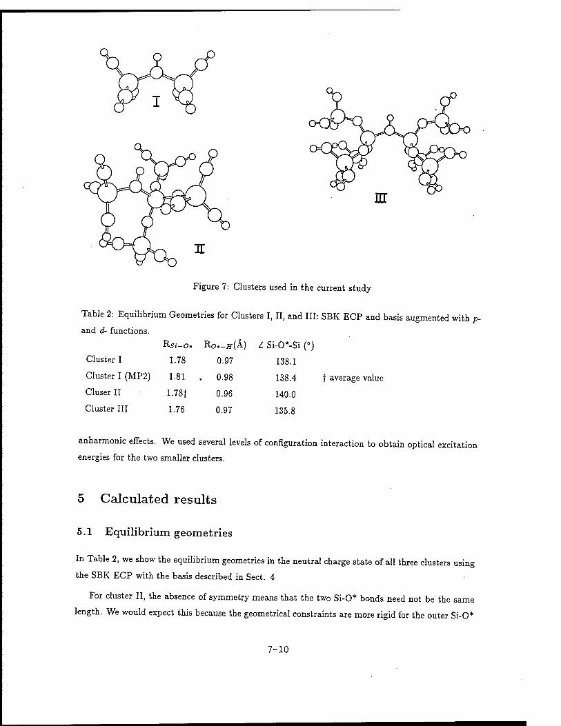
Figure 7: Clusters used in the current study
Table 2: Equilibrium Geometries for Clusters I, II, and III: SBK ECP and basis augmented with p-
and d- functions.
Rsi-o. Ro.-jf(Ä) Z Si-0*-Si (°)
Cluster I 1.78 0.97 138.1
Cluster I (MP2) 1.81 . 0.98 138.4 f average value
Cluser II 1.78f 0.96 140.0
Cluster III 1.76 0.97 135.8
anharmonic effects. We used several levels of configuration interaction to obtain optical excitation
energies for the two smaller clusters.
5 Calculated results
5.1 Equilibrium geometries
In Table 2, we show the equilibrium geometries in the neutral charge state of all three clusters using
the SBK ECP with the basis described in Sect. 4
For cluster II, the absence of symmetry means that the two Si-O* bonds need not be the same
length. We would expect this because the geometrical constraints are more rigid for the outer Si-O*
7-10
Table 3: Changes in atomic charges for Clusters I, II, and III: SBK ECP and basis augmented with
p- and d- functions. The two values are for Mulliken and (Löwdin) population analysis
AQH (e) AQ 0*(e)
Cluster I 0.37 (0.30) 0.01 (0.11)
Cluser II 0.35 (0.28) 0.0 (0.15)
Cluster III 0.38 (0.31) 0.0 (0.17)
Table 4: Vibrational spectrum for the proton in Si02: Cluster I (all values in eV)
Mode hu XJJ y# z#
O-H stretch 0.338 0.0 0.0 0.94
in-plane rock 0.107 0.92 0.0 0.0
out-of-plane rock i 0.108 0.0 0.96 0.0
bond. In this case the difference is 0.4 Ä. Otherwise, the results are quite similar across clusters
and compare well with the previous results using the 6-31G** basis. We show the differences of
charge on each of the central atoms in Table 3. These differences were calculated by considering the
isolated clusters in the neutral charge states without the extra hydrogen atom.
Even though this is called a proton, the calculated charges show clearly that the charge is
delocalized significantly, In fact, the Löwdin population analysis indicates that the oxygen atom
picks up more positive charge than the hydrogen atom. We should note, however, that charge
assignments are somewhat arbitrary, and should only be used for qualitative arguments. In Fig.
9 we show the potential surfaces we obtained for H+ and H° motion for clusters I and II. For all
potential surfaces, the cluster is rigid; only R0.H is altered. Note that for the H+ motion, the
asymptotic state is a proton and a neutral Si207H7 cluster, rather than the correct hydrogen atom
and self-trapped hole. For our purposes, the calculation of the first three vibrational states, this will
probably make no difference, (see Sect. 7.) For Cluster I, this result is in reasonable quantitative
agreement with Ref. [11]. Our proton binding energy is actually larger by 3 eV. This is reduced
dramatically in the MP2 approximation, leading to a surface that is very close to that of Ferreira
et al. Furthermore, the surfaces for clusters I and II are almost identical. We obtain a better
appreciation of this similarity from the vibrational analysis. In Table 4 we show the frequencies
of the three principle proton vibrational modes involving the central hydrogen atom for cluster I.
Because these were obtained from a full Hessian calculation, we obtained the components of the
normal modes as well. These are also given in Table 4. Note the large components on the central
hydrogen atom, justifying our claim that these are the principle proton modes. The most important
7-11
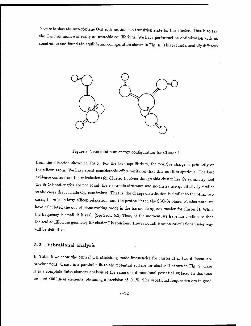
feature is that the out-of-plane O-H rock motion is a transition state for this cluster. That is to say,
the C2„ minimum was really an unstable equilibrium. We have performed an optimization with no
constraints and found the equilibrium configuration shown in Fig. 8. This is fundamentally different
Figure 8: True minimum energy configuration for Cluster I
from the situation shown in Fig.5. For the true equilibrium, the positive charge is primarily on
the silicon atom. We have spent considerable effort verifying that this result is spurious. The best
evidence comes from the calculations for Cluster II. Even though this cluster has d symmetry, and
the Si-0 bondlengths are not equal, the electronic structure and geometry are qualitatively similar
to the cases that include C2t/ constraints. That is, the charge distribution is similar to the other two
cases, there is no large silicon relaxation, and the proton lies in the Si-O-Si plane. Furthermore, we
have calculated the out-of-plane rocking mode in the harmonic approximation for cluster II. While
the frequency is small, it is real. (See Sect. 5.2) Thus, at the moment, we have fair confidence that
the real equilibrium geometry for cluster I is spurious. However, full Hessian calculations under way
will be definitive.
5.2 Vibrational analysis
In Table 5 we show the central OH stretching mode frequencies for cluster II in two different ap-
proximations. Case I is a parabolic fit to the potential surface for cluster II shown in Fig. 9. Case
II is a complete finite element analysis of the same one-dimensional potential surface. In this case
we used 400 linear elements, obtaining a precision of 0.1%. The vibational frequencies are in good
7-12
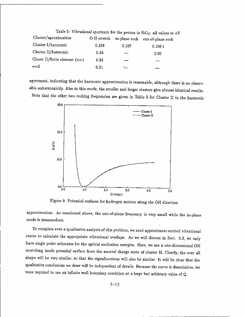
Table 5: Vibrational spectrum for the proton in Si02: all values in eV Cluster/aproximation
Cluster I/harmonic
Cluster II/harmonic
Cluser II/finite element (n=l
n=2
O-H stretch in-plane rock out-of-plane rock
0.338 0.107 0.108 i
0-34 — 0.02
0.34 — _
0.31 — _
agreement, indicating that the harmonic approximation is reasonable, although there is an observ-
able anharmonicity. Also in this mode, the smaller and larger clusters give almost identical results.
Note that the other two rocking frequencies are given in Table 5 for Cluster II in the harmonic
30.0
20.0
10.0
1.0 2.0 3.0 Q (Angs.)
4.0 5.0
Figure 9: Potential surfaces for hydrogen motion along the OH direction
approximation. As mentioned above, the out-of-plane frequency is very small while the in-plane
mode is intermediate.
To complete even a qualitative analysis of this problem, we need approximate excited vibrational
states to calculate the appropriate vibrational overlaps. As we will discuss in Sect. 5.3, we only
have single point estimates for the optical excitation energies. Here, we use a one-dimensional OH
stretching mode potential surface from the neutral charge state of cluster II. Clearly, the over all
shape will be very similar, so that the eigenfunctions will also be similar. It will be clear that the
qualitative conclusions we draw will be independent of details. Because the curve is dissociative, we
were required to use an infinite wall boundary condition at a large but arbitrary value of Q.
7-13
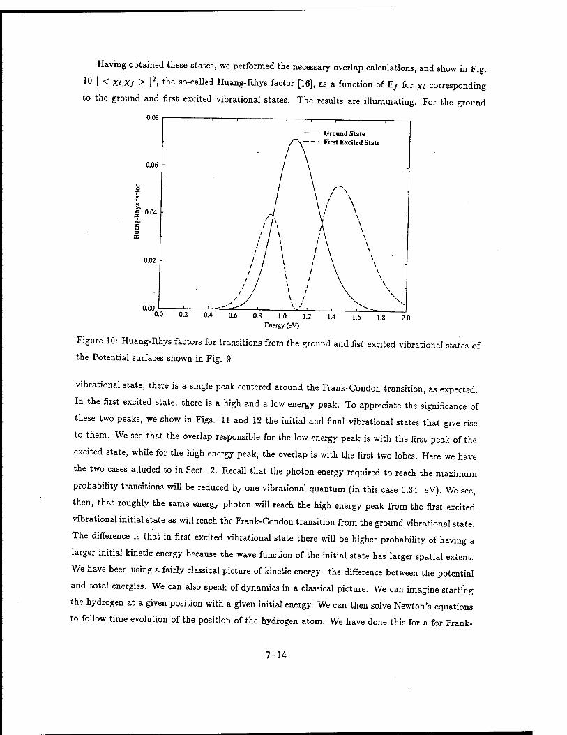
Having obtained these states, we performed the necessary overlap calculations, and show in Fig.
!0 | < Xikf > |2, the so-called Huang-Rhys factor [16], as a function of Ef for Xi corresponding
to the ground and first excited vibrational states. The results are illuminating. For the ground
0.08
0.06
| 0.04
0.02
0.00
— Ground State First Excited State
Figure 10: Huang-Rhys factors for transitions from the ground and fist excited vibrational states of
the Potential surfaces shown in Fig. 9
vibrational state, there is a single peak centered around the Frank-Condon transition, as expected.
In the first excited state, there is a high and a low energy peak. To appreciate the significance of
these two peaks, we show in Figs. 11 and 12 the initial and final vibrational states that give rise
to them. We see that the overlap responsible for the low energy peak is with the first peak of the
excited state, while for the high energy peak, the overlap is with the first two lobes. Here we have
the two cases alluded to in Sect. 2. Recall that the photon energy required to reach the maximum
probability transitions will be reduced by one vibrational quantum (in this case 0.34 eV). We see,
then, that roughly the same energy photon will reach the high energy peak from the first excited
vibrational initial state as will reach the Frank-Condon transition from the ground vibrational state.
The difference is that in first excited vibrational state there will be higher probability of having a
larger initial kinetic energy because the wave function of the initial state has larger spatial extent.
We have been using a fairly classical picture of kinetic energy- the difference between the potential
and total energies. We can also speak of dynamics in a classical picture. We can imagine starting
the hydrogen at a given position with a given initial energy. We can then solve Newton's equations
to follow time evolution of the position of the hydrogen atom. We have done this for a for Frank-
7-14
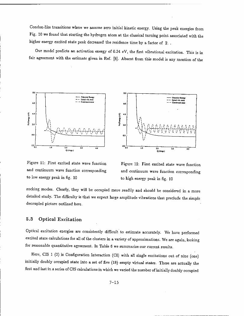
Condon-like transitions where we assume zero initial kinetic energy. Using the peak energies from
Fig. 10 we found that starting the hydrogen atom at the classical turning point associated with the
higher energy excited state peak decreased the residence time by a factor of 2. .
Our model predicts an activation energy of 0.34 eV, the first vibrational excitation. This is in
fair agreement with the estimate given in Ref. [8]. Absent from this model is any mention of the
5 "
£ 2.0 ■
Potential Energy Iftititl vib. stale Continuum stale
i '
Q (Angv)
? 40
ft
Potential Energy — Initial vib. stale — Continuum tute
''*• A '"> •', !\ !\ ;' '"' •'■ /' .'; P '; ■
10 Q(Angs.)
Figure 11: First excited state wave function
and continuum wave function corresponding
to low energy peak in fig. 10
Figure 12: First excited state wave function
and continuum wave function corresponding
to high energy peak in fig. 10
rocking modes. Clearly, they will be occupied more readily and should be considered in a more
detailed study. The difficulty is that we expect large amplitude vibrations that preclude the simple
decoupled picture outlined here.
5.3 Optical Excitation
Optical excitation energies are consistently difficult to estimate accurately. We have performed
excited state calculations for all of the clusters in a variety of approximations. We are again, looking
for reasonable quantitative agreement. In Table 6 we summarize our current results.
Here, CIS 1 (2) is Configuration Interaction (CI) with all single excitations out of nine (one)
initially doubly occupied state into a set of five (18) empty virtual states. These are actually the
first and last in a series of CIS calculations in which we varied the number of initially doubly occupied
7-15
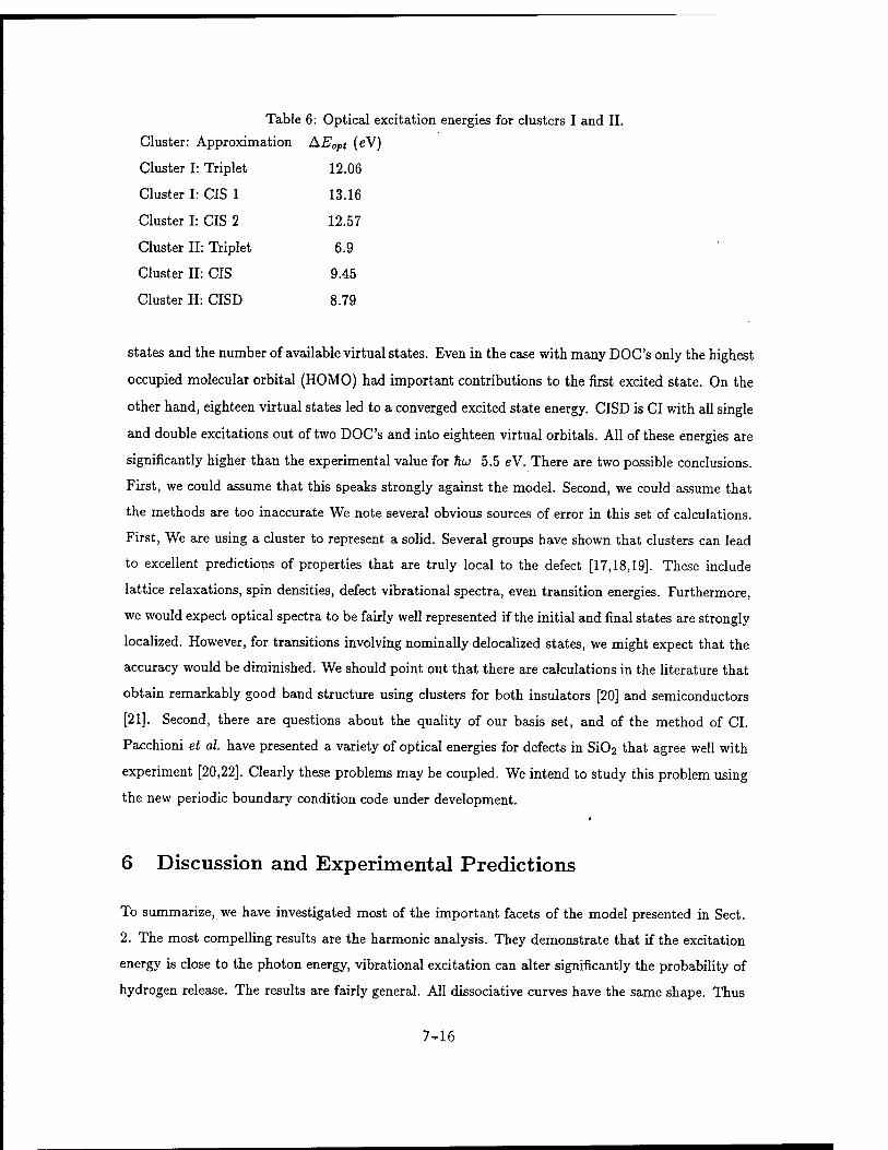
Table 6: Optical excitation energies for clusters I and II.
Cluster: Approximation AEopt (eV)
Cluster I: Triplet 12.06
Cluster I: CIS 1 13.16
Cluster I: CIS 2 12.57
Cluster II: Triplet 6.9
Cluster II: CIS 9.45
Cluster II: CISD 8.79
states and the number of available virtual states. Even in the case with many DOC's only the highest
occupied molecular orbital (HOMO) had important contributions to the first excited state. On the
other hand, eighteen virtual states led to a converged excited state energy. CISD is CI with all single
and double excitations out of two DOC's and into eighteen virtual orbitals. All of these energies are
significantly higher than the experimental value for fiu 5.5 eV. There are two possible conclusions.
First, we could assume that this speaks strongly against the model. Second, we could assume that
the methods are too inaccurate We note several obvious sources of error in this set of calculations.
First, We are using a cluster to represent a solid. Several groups have shown that clusters can lead
to excellent predictions of properties that are truly local to the defect [17,18,19]. These include
lattice relaxations, spin densities, defect vibrational spectra, even transition energies. Furthermore,
we would expect optical spectra to be fairly well represented if the initial and final states are strongly
localized. However, for transitions involving nominally delocalized states, we might expect that the
accuracy would be diminished. We should point out that there are calculations in the literature that
obtain remarkably good band structure using clusters for both insulators [20] and semiconductors
[21]. Second, there are questions about the quality of our basis set, and of the method of CI.
Pacchioni et al. have presented a variety of optical energies for defects in Si02 that agree well with
experiment [20,22]. Clearly these problems may be coupled. We intend to study this problem using
the new periodic boundary condition code under development.
6 Discussion and Experimental Predictions
To summarize, we have investigated most of the important facets of the model presented in Sect.
2. The most compelling results are the harmonic analysis. They demonstrate that if the excitation
energy is close to the photon energy, vibrational excitation can alter significantly the probability of
hydrogen release. The results are fairly general. All dissociative curves have the same shape. Thus
7-16

the effects will differ quantitatively but not qualitatively. This quantitative difference could, of course
be so large as to preclude practical observation of temperature activated capture. If, for example
the ground state minimum were coincident with the flat section of the dissociative curve, then
promotion to an excited vibrational state could have very little effect because there would be no state
close to the excitation energy with significant vibrational overlap. We have performed deuterium
studies with inconclusive results. We would predict small increases in activation energies, but no
dramatic effects. However, we can make several experimental predictions that can be investigated
immediately. First, any technique for introducing electrons into the S1O2 conduction band should
lead to proton annihilation at any temperature. A straightforward experiment would be avalanche
electron injection. Second, we recommend a spectroscopic study of the excitation energy, as this
could delineate between the kinetic and the energetic mechanism. If the photon energy is close to,
but smaller than, the Frank-Condon transition energy,i?F_c, an increase in fiu could well lead to
an increase in low temperature proton annihilation. However, if the kinetic argument holds, and
hu m Ep-c, then increasing Tiu could have a variety of effects. One should be able to map the
vibrational probability as a function of energy for the excited vibrational state.
7 Future extensions
In Sect. 1, we outlined several interesting problems in the protonated buried oxide system. We have
reported here the progress made on one of them. Our future plans can be segregated into plans for
completing the analysis of this model, and plans to study other interesting problems.
7.1 Electron capture: future studies
We have put forward and studied a model for electron capture under 5.5 eV light that relies on
knowing both the vibrational spectrum and wave functions and the electronic spectrum to within
0.5 eV.We have finished the vibrational analysis for the case of an accurate positive charge state
potential, and a model excited state potential— that for the neutral charge state. We plan to
complete a careful study of the excited state going beyond the standard CI method to include multi-
configuration SCF (MCSCF) calculations with a variety of sets of basis functions. To date, the best
optical calculations from clusters are from Pacchioni and coworkers [20,22]. This group has used
multi-reference singles and doubles CI (MRDCI). Part of our work will be to assess the need for
such methods by repeating some of the Pacchioni calculations with MCSCF. When we are satisfied
that we understand the calculational requirements for this system, we will obtain a complete excited
7-17

state potential surface. This, of course will be crucial for testing the model theoretically. If we
obtain reliable excitation energies that disagree with the experimental values, we will be forced to
abandon the cluster model. If the calculated energies are close to the experimental values, then we
plan a careful calculation of the electronic part of the optical transition probability using the results
from the CI calculations. We will be especially interested in the effect of hydrogen motion on the
electronic transition strength. It may turn out that rocking motion will be especially important.
Another, possibly important, piece of this study will be the effect of local strain on the calculated
potential surfaces. For many years Revesz has contended that local compressive strain should lead
to higher reactivity. We will study clusters that have built in strain.
All of the work involving finite clusters should be finished over the five months. At the same
time, we will be developing our periodic boundary condition-code to eliminate the effects of cluster
termination. When this is available, we will use it on an a-quartz model of the proton problem.
These calculations should lead to some definitive statements about the utility of our model.
7.2 Other proton-related problems
There are three very interesting and related problems we would like to pursue. We would like
to understand the mechanism that transforms molecular hydrogen to protons in buried oxides.
Specifically, we would like to study the possible cracking sites that would lead from H2 to either
H° or directly to the proton species. In the SERP, I will outline in detail, our ideas for these
calculations. We also want to understand why this positively charged species is so stable. We are
especially interested in why, in buried oxides, the proton does not acquire an electron from the
substrate. Again, in the SERP, I will outline in detail our plans. Finally, Vanhuesden has shown
recently that the formation of protons is very sensitive to the rate of cooling after the 600° anneal
in forming gas. This last observation may well tie together the previous two questions. That is, the
physics of proton formation and of proton stability will dictate the rate of annihilation as a function
of cooling rate.
Acknowledgments
The author thanks Dr. K. Vanheusden for extremely useful discussions of the experiments prior
to publication. He also thanks Dr. S. P. Kama and Profs. H. Kurtze, B. Kirtman, and W. B. Fowler
for valuable comments and critiques during the course of this work. He gratefully acknowledges the
support of Phillips Laboratory VT/MR branch, especially of Drs. Walter Shedd, R. Pugh and B. K.
Singaraju, during his tenure as an AFOSR Summer Fellow. Finally, he acknowledges the use of the
7-18
computational resources at the Albuquerque Resource Center for many of the calculations presented
herein.
REFERENCES
1. G. E. Davis, H. R. Hite, T. G. W. Blake, C. E. Chen, and H. W. Lam, IEEE Trans. Nuc.
Sei. NS-32, 4432 (1985).
2. J. P. Colinge, Electron. Lett. 22, 187 (1985).
3. R. E. Stahlbush, G. J. Campisi, J. B. McKitterick, W. P. Maszara, P. Roitman, and G. A. Brown,
IEEE Trans. Nucl. Sei. NS-39, 2086 (1992).
4. K. Vanheusden, and A. Stesmans, Appl. Phys. Lett. 64, 2575 (1994).
5. K. Vanheusden, W. L. Warren, R. A. B. Devine, D. M. Fleetwood, J. R. Schwank, M. R.
Shaneyfelt, P. S. Winokur, and Z. J. Lemnios, Nature 386, 587 (1997).
6. K. Vanheusden, W. L. Warren, and R. A. B. Devine, J. Non-Cryst. Solids 216, 116 (1997).
7. D. L. Griscom, D. B. Brown, and N. S. Saks, in The Physics and Chemistry of Si02 and the
Si-SiC-2 Interface, edited by C. R. Helms, and B. E. Deal, (Plenum, New York, 1988), p. 287.
8. K. Vanheusden, W. L. Warren, D. W. Fleetwood, S. P. Kama, A. M. Ferreira, R. D. Pugh, C. P.
Brothers, B. K. Singaraju, R. A. B. Devine, and A. H. Edwards, Appl. Phys. submitted.
9. R. A. B. Devine, Priate communication.
10. A. H. Edwards, J. A. Pickard, R. E. Stahlbush, J. Non-Cryst. Solids 179, 148 (1994).
11. A. M. Ferreira, S. P. Kama, C. P. Brothers, R. D. Pugh, B. K. Singaraju, K. Vanheusden, W. L.
Warren, and R. A. B. Devine, in Amorphous and Crystalline Insulating Thin Films, edited by W. L.
Warren, R. A. B. Devine, M. Matsumura, S. Cristoloveanu, Y. Homma, and J. Kanicki, (Materials
Research Society, Pittsburgh, 1997), p. 187.
12. A. H. Edwards, and G. Germann, Nucl. Instr. and Meth. in Phys. Res. B 32, 238 (1988).
13. A. Yokozawa, and Y. Miyamoto, Phys. Rev. B 55, 13783 (1997).
14. M. W. Schmidt, K. K. Baldridge, J. A. Boatz, S. T. Elbert, M. S. Gordon, J. H. Jensen, S.
Koseki, N. Natsunaga, K. A. Nguyen, S. J. Su, T. L. Windus, M. Dupuis, and J. A. Mongtomery,
J. Comput. Chem. 14, 1347 (1993).
15. W. J. Stevens, H. Basch, and M. Krauss, J. Chem. Phys. 81, 6026 (1984).
16. K. Huang, and A. Rhys, Proc. R. Soc. London Ser. A 204, 406 (1950).
17. A. H. Edwards, Phys. Rev. B36, 9638 (1987).
18. M. Cook, and C. T. White, Phys. Rev. Lett. 59, 1741 (1987).
19. K. C. Snyder, and W. B. Fowler, Phys. Rev. B48, 13238 (1993).
20. G. Pacchioni, and G. Ierano, Phys. Rev. Lett, in press (1997).
7-19

21. A. Lizon-Nordstrom, and F. Yndurain, Solid State Commun. 94, 335 (1995).
22. G. Pacchioni, and G. Ierano, Phys. Rev. B56, 1 (1997).
7-20
MODELING THE MAGNETOSPHERIC MAGNETIC FIELD
Gary M. Erickson Associate Professor
Center of Space Physics
Boston University 725 Commonwealth Avenue
Boston, MA 02215
Final Report for: Summer Research Program
Phillips Laboratory
Sponsored by: Air Force Office of Scientific Research
Boiling Air Force Base, Washington, DC
And
Phillips Laboratory
August, 1997
8-1
MODELING THE MAGNETOSPHERIC MAGNETIC FIELD
Gary M. Erickson Research Assistant Professor
Center for Space Physics Boston University
Abstract
Following the formalism developed by Heinemann and collegues, development of a nu-
merical method for obtaining the three-dimensional, equilibrium, magnetospheric magnetic
field has begun. Expressing the distributed currents of the magnetospheric plasma in terms
of an effective magnetization Me//, the magnetic scalar potential ip is found as a solution
of Poisson's equation. The magnetic field is B = fiQ (—V^ + Me//) in MKS units, just as
in an ordinary diamagnetic material. In this first stage of development, numerical solutions
have been found in a closed rectangular geometry, with symmetry about the equatorial and
noon-midnight meridian planes, and isotropic pressure with an assumed distribution in the
equatorial plane.
8-2

MODELING THE MAGNETOSPHERIC MAGNETIC FIELD
Gary M. Erickson
Motivation
In support of spacecraft operations the Air Force has a long-term commitment to understand
the near-Earth space environment. Energetic particles, both those trapped and energized
within the magnetosphere and those arriving from the sun, have deleterious efects on space
operations. Electron precipitation and Joule heating increases ionospheric densities and tem-
peratures, which can interfere with radar, communications, and can result in increased drag
on low-altitude spacecraft. Understanding the coupling between the solar wind, magneto-
sphere, and ionosphere is crucial if the time evolution of the near-Earth natural environment
is to be specified or predicted.
There are two basic, complementary approaches to physics-based modeling of the near-Earth
space environment: global MHD and regional-modular. Global MHD is very good at obtain-
ing the global topology resulting from the flow of solar wind past Earth's magnetosphere.
It can follow highly time-dependent (including shock propagation) evolution of the magne-
tosphere, whereas a regional-modular approach does not. However, MHD does not resolve
boundary layers, the codes are diffusive, and simulations will wander rapidly away from
reality during a simulation. Tuning is a difficult problem and data assimilation may be an
unsolvable problem for MHD models.
For space weather operations the advantages of a regional-modular approach are in com-
putational speed at higher spatial resolution, the ability to fine-tune the model to specific
conditions, and, especially, data assimilation. For basic research the regional-modular ap-
proach complements global MHD by permitting higher resolution, incorporation of realistic
boundary layers, and control of parameters external to the issue of investigation.
The central criticism of the regional-modular approach has concerned the "spine" or com-
putational backbone; specifically, how does one get the various, often disparate, regional
models to talk to each other? Heinemann and collegues [Heinemann and Pontius, 1990,
8-3
1991; Heinemann et al., 1994; Heinemann and Erickson, 1997] have derived expressions
for the "effective magnetization" of the magnetospheric plasma, permitting solution for the
global magnetospheric magnetic field from Ampere's law using the magnetic scalar potential.
Using this formulation, cross-module communication within the regional-modular approach
is greatly simplified. The difficulty is that the effective magnetization depends explicitly on
the magnetic field. An iterative, numerical approach is required to find the magnetospheric
magnetic field and currents.
Development of a numerical method, based on the "effective magnetization" formulation, to
obtain the three-dimensional, equilibrium, magnetospheric magnetic field has begun. In this
first phase of development, solutions have been obtained in a rectangular, magnetospheric
geometry. Vacuum solutions were obtained for various strengths of the normal component
of the magnetic field through the tailward boundary of the modeling region. For non-zero
normal component, these solutions contain a magnetic neutral line within the magnetotail.
Non-vacuum solutions were obtained for zero normal component. Solutions were obtained
with isotropic plasma pressures up to about one-quarter of that in Earth's magnetotail. To
proceed toward more realistic magnetospheric solutions, in the next phase of development
the rectangular geometry must be abandoned for a more realistic magnetopause shape, and
the tailward boundary condition must be constructed with finite plasma pressure and normal
magnetic field component.
Methodology
For illustration of the "effective magnetization" formulation assume isotropic pressure and
neglect inertia! currents. The magnetic configuration at any instant will be in quasi-static
equilibrium. In MKS units the magnetic field B, plasma pressure P, and plasma current J
are related by
JxB = VP (1)
where
V x B = fi0 J (2)
8-4
and
V-B = 0 (3)
The procedure is to solve for J in (1) in terms of B. The solution for (1) is just Vasyliunas'
[1970] formula (see Heinemann and Pontius [1990])
j(«) = vf/ x ds
~B x VP (4)
The integral is performed along B from the equator to x. The equatorial properties are
determined from advection of the plasma. Since J is divergence free, (4) can be written as
a curl of an effective magnetization Me//
J = V x Me// (5)
where in the present case
Me//(x) = -Pv/X| (6)
and in analogy with ordinary diamagnetic media
B = ^o(-VV' + Me//) (7)
where iß = ij)int + ipM] 4>int is the magnetic scalar potential given by the multipole represen-
tation of the IGRF [Barker et al, 1986]; and if>M is the contribution from the distributed
(plasma) currents. Taking the divergence of (7), ifj satisfies
V2V>M = V-Me// (8)
noting that V^mt = 0 away from Earth's center.
Iterating between (6) and (8) yields the solution for B, given by (7), consistent with the
plasma currents, i.e., satisfying force balance. This illustrates the general approach we take
to computing magnetic field configurations consistent with the plasma currents. The source
terms (4)-(6) have been generalized for anisotropic pressure [Heinemann and Pontius, 1991],
inclusion of steady-state inertia! currents [Heinemann et al, 1994], and finite-Larmour-radius
8-5
effects [Heinemann and Erickson, 1997]. Techniques are also provided for generalization to
treat currents on open field lines. These generalizations permit modeling of the entire, open
magnetospheric configuration, including its boundary layers.
Boundary conditions on (8) are given at the magnetopause and at a mid-tail cross-section.
Boundary conditions along the magnetopause can be specified using the technique of Toffo-
letto and Hill [1993]. The plasma distribution within the magnetopause and tail boundary is
self-consistently derived using an M-I coupled convection code such as the Rice Convection
Model [e.g., Erickson et al, 1991]. Following the techniques of Onsager et al. [1993] to ob-
tain plasma distributions and Heinemann and Erickson [1997] to compute current associated
with the plasma-sheet boundary layer, a convection model can be extended into the far tail.
In principle, plasma transport can be modeled throughout the magnetosphere, including the
boundary layers.
Describing plasma currents in terms of the plasma magnetization and solving directly for the
magnetic scalar potential has several advantages over other methods. Lagrangian methods,
such as developed for the fusion community and recently adapted for magnetospheric appli-
cations [Cheng, 1995], require specification of a flux surfaces as boundary conditions. Such
specification is not possible when modeling the open magnetosphere. The "effective magne-
tization" approach includes field-aligned currents self-consistently. Eqns. (4)-(6), and thus
(8), contain the current perpendicular and parallel to B. Other methods, based on solution
of the momentum equation (1), know only of the perpendicular current. Finally, non-MHD
effects, such as finite-Larmour-radius effects [Heinemann and Erickson, 1997] can be incor-
porated into this formulation.
Numerical Approach
An alternating-directions-implicit (ADI) [e.g., Varga, 1959] is used to solve (8) for given
V • Me//(B). Me//(B) is then recomputed, and (8) is solved again. This loop repeats until
convergence is obtained.
8-6
For the first phase in the development of this approach to magnetospheric modeling, solutions
of (8) were sought for a rectangular magnetospheric geometry. The normal magnetic field
component Bn = 0 along the dayside face located at 10.5 RE sunward of the Earth, and
at the dawn, dusk, north and south faces making a square cross-section 40 RE on a side.
The tailward face was placed 60.5 RE behind the Earth. (RE is an Earth radius.) To test
the basic logic of the code and ADI solver, vacuum (Me// = 0) solutions were sought for
various values of Bn along the tail boundary. (Bn into the simulation box in the northern
hemisphere, and out in the southern hemisphere.) For non-vacuum solutions, the magnetic
field was assumed closed within the rectangular boundary; Bn = 0 on all faces. The pressure
was specified on the equatorial plane such as to be constant near Earth, fall off as |x|~1-2
down the tail, and vanish at the dayside and tailward faces.
Results
Vacuum solutions were obtained for various values of Bn on the tailward face of the simulation
box. For Bn ^ 0, the solution contained a magnetic neutral line within the simulation box.
A neutral line must form in this case. As there is no north-south component of the field on
the tailward face, Earth's magnetic field must close within the simulation box. At the same
time, the boundary condition on the tailward face must be met. A neutral line is required
to satisfy both conditions.
Non-vacuum solutions were obtained for varying amounts of plasma pressure up to about
one-quarter of that in Earth's central plasma sheet. Solutions were sought for Bn = 0 on the
tailward face. Adding pressure to the tail would normally cause the field to become more
taillike. However, the Bn = 0 boundary condition does not permit this to happen. Instead,
the field has to undergo an unnatural distortion in the tailward portion of the simulation box.
Starting from the vacuum solution, convergence was fast as magnetic flux had nowhere to go.
Unfortunately, as the pressure exceeded about one-quarter that in Earth's central plasma
sheet, the distortions were becoming too large and the field-line tracer for computing Me//
had difficulties. Rather than adding additional overhead to the numerical code to deal with
8-7

this (unrealistic) behavior, the solver was declared to pass its first phase of development.
Conclusion
The first phase in the development of an equilibrium magnetospheric magnetic field solver
based on the "effective magnetization" approach has been completed successfully. In this
first phase of development, numerical solutions for (8) were obtained in a closed, rectangular,
magnetospheric geometry. To proceed toward realistic magnetospheric solutions, the next
phase of development will be to generalize the numerical code for realistic magnetopause
shapes and Bn ^ 0 anywhere, as well as both nonzero pressure and Bn on the tailward
boundary.
References
Barker, F. S., D. R. Barraclough, V. P. Golovkov, P. J. Hood, F. J. Lowes, W. Mundt, N.
W. Peddie, Qi Gui-zhong, S. P. Srivastava, R. Whitworth, D. E. Winch, T. Yukutake,
and D. P. Zidarov, International geomagnetic reference field revision 1985, EOS Tran.
AGU, 67, 523, 1986.
Cheng, C. Z., Three-dimensional equilibrium with isotropic pressure, Geophys. Res. Lett.,
22, 2401, 1995.
Erickson, G. M., R. W. Spiro, and R. A. Wolf, The physics of the Harang discontinuity, J.
Geophys. Res., 96, 1633, 1991.
Heinemann, M., and G. M. Erickson, Field-aligned currents and parallel potential fields in
the plasma sheet boundary layer, J. Geophys. Res., submitted, 1997.
Heinemann, M., and D. H. Pontius, Jr., Representation of currents and magnetic fields in
isotropic magnetohydrostatic plasma, J. Geophys. Res., 95, 251, 1990.
Heinemann, M., and D. H. Pontius, Jr., Representation of currents and magnetic fields in
anisotropic magnetohydrostatic plasma, 2. General theory and examples, J. Geophys.
Res., 96, 17,609, 1991.
Heinemann, M., G. M. Erickson, and D. H. Pontius, Jr., Inertia! currents in isotropic plasma,
8-8
/. Geophys. Res., 99, 8635, 1994.
Onsager, T. G., C. A. Kletzing, J. B. Austin, and H. MacKiernan, Model of magnetosheath
plasma in the magnetosphere: cusp and mantle particles at low-altitudes, Geophys. Res.
Lett, 20, 479, 1993.
Toffoletto, F. R., and T. W. Hill, A nonsingular model of the open magnetosphere, J.
Geophys. Res., 98, 1339, 1993.
Varga, R. S., Iterative Numerical Analysis. University of Pittsburgh, Pittsburgh, Pa., 1959.
Vasyliunas, V. M., Mathematical models of magnetospheric convection and its coupling to
the ionosphere, in Particles and Fields in the Magnetosphere, edited by B. M. McCormac,
D. Reidel, Hingham, MA, p. 60, 1970.
8-9
FOCAL POINT ACCURACY ASSESSEMENT OF AN OFF-AXIS SOLAR CONCENTRATOR
H. Ghoneim Associate Professor
Department of Mechanical Engineering
Rochester Institute of Technology One Lomb Memorial Drive
Rochester, NY 14623
Final Report for: Summer Research Program
Phillips Laboratory
Sponsored by: Air Force Office of Scientific Research
Boiling Air Force Base, Washington, DC
And
Phillips Laboratory
August, 1997
9-1
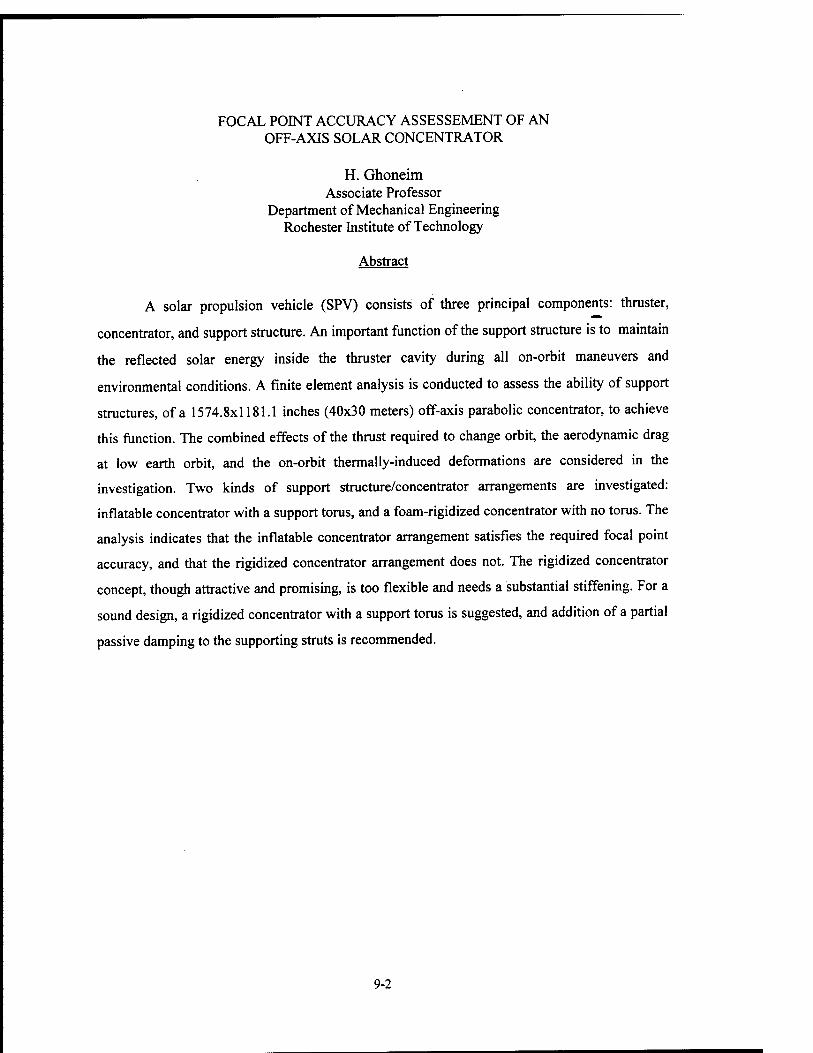
FOCAL POINT ACCURACY ASSESSEMENT OF AN OFF-AXIS SOLAR CONCENTRATOR
H. Ghoneim Associate Professor
Department of Mechanical Engineering Rochester Institute of Technology
Abstract
A solar propulsion vehicle (SPV) consists of three principal components: thruster,
concentrator, and support structure. An important function of the support structure is to maintain
the reflected solar energy inside the thruster cavity during all on-orbit maneuvers and
environmental conditions. A finite element analysis is conducted to assess the ability of support
structures, of a 1574.8x1181.1 inches (40x30 meters) off-axis parabolic concentrator, to achieve
this function. The combined effects of the thrust required to change orbit, the aerodynamic drag
at low earth orbit, and the on-orbit thermally-induced deformations are considered in the
investigation. Two kinds of support structure/concentrator arrangements are investigated:
inflatable concentrator with a support torus, and a foam-rigidized concentrator with no torus. The
analysis indicates that the inflatable concentrator arrangement satisfies the required focal point
accuracy, and that the rigidized concentrator arrangement does not. The rigidized concentrator
concept, though attractive and promising, is too flexible and needs a substantial stiffening. For a
sound design, a rigidized concentrator with a support torus is suggested, and addition of a partial
passive damping to the supporting struts is recommended.
9-2
FOCAL POINT ACCURACY ASSESSEMENT OF AN OFF-AXIS SOLAR CONCENTRATOR
H. Ghoneim
Introduction
The solar propulsion concept (SPC) is an attractive technique for orbital-transfer applications.
Solar propulsion vehicles, in general, are efficient, relatively cheap, reusable and versatile {1}.
A solar propulsion vehicle (SPV) consists of three principal components (Fig. 1): concentrator,
thruster (engine), and support structure. The concentrator gathers, focuses and concentrates the
sun's energy into a thruster cavity. The thruster captures the solar energy and converts it into heat
which expands a single hydrogen working fluid through a nozzle, producing the propulsive
thrust. The support structure (tori and truss members) rigidly connects the concentrators to the
thruster. The only relative motion allowed between the support structure and the thruster is the
slewing motion about the z axis, in order to maintain the reflectors directed towards the sun. A
turntable provides such slewing maneuver. An important function of the support structure which
is vital to the success of the SPC is to maintain the reflected sun's rays focused inside the thruster
cavity during all on-orbit maneuvers and environmental conditions.
The objective of this work is to investigate the ability of candidate support structures to achieve
the above-mentioned function. The investigation is carried out using the ANSYS finite element
software. The subject of the investigation is the SPV (Fig. 1) with two parabolic off-axis
concentrators supported by three struts each (two long struts and one short). Two concentrator
arrangements are examined: inflatable thin-film concentrator (reflector/canopy arrangement)
with a support torus as shown in the Fig. 1, and a foam-rigidized concentrator. The latter is
viewed as an alternative arrangement which overcomes the problem of the make-up gas needed
to maintain inflation and which improves the optical quality of the concentrator. Three on-orbit
loads are considered for the investigation: 1) the thrust due to firing the thruster to change orbit,
2) the aerodynamic drag force at low earth orbit (LEO), and 3) thermal load due to temperature
differential with respect to earth temperature and temperature gradient across the struts and torus
cross sections. The solar wind, plume impingement and the sun tracking control forces (roll and
yaw torque) are not considered in the present investigation. Previous preliminary analyses
suggest that these forces have little impact on the focal point accuracy {2}.
9-3
Characteristics of the Solar Propulsion Vehicle
Figure 2 shows the basic geometry, dimensions and coordinate system of the off-axis
concentrator {2} adopted for the current investigation. This concentrator gives a theoretical peak
concentration ratio of 12,560 which satisfies the minimum required concentration ratio of
10,000. The concentrator also provides the desired 1 MWatt solar power.
Both the struts and tori of the support structure are made of inflated, rigidized, space-cured
carbon-epoxy composite beams. These are thin-walled tubes consisting of unidirectional M40J
carbon fibers composite prepreg with a lay-up of [±30/0/90/±30]. The carbon-fiber composites
enjoy a near-zero coefficient of thermal expansion (CTE) and a high specific stiffness. The
outside diameters of the tubular struts and torus are assumed to be 13 and 7 inches, respectively.
A 0.015-inch wall thickness is assigned for both the torus and struts. The reflector as well as the
canopy is constructed from a 0.0005-inch thin film polyimide material. Polyimide films have
material properties that are superior to those of other film materials and they retain their
properties over a wide range of temperature {3}. The rigidized concentrator is assumed to be
made of a 0.0625-inch thick (LaRC-CPl) polyimide film foam-rigidized with EPON Resin 828
epoxy. It has excellent adhesive properties and consequently is viewed as a good material for this
specific application. The relevant material properties adopted for the current analysis are shown
in Table 1.
Graphite-Epoxy composite Polyimide
(6FDA+APB) polyimide
(LaRC-CPl) Foam Epoxy
(with glass fillers)
Modulus of elasticity, E xl06(psi)
17.21
0.4
0.315
0.15
Poisson's ratio
0.3
0.4
0.4
0.35
CTExlO-6
(in/in-°F)
0.1
27.5
Density (lb/ft3)
102
60
90
50
Table 1 Relevant Material Parameters
As mentioned before, three combined loads are considered in the current study: thrust,
aerodynamic drag, and thermal loads. It is assumed that the maximum output of the thruster is a
100-lb force. This force will be used to transfer the fully-loaded SPV, with a total mass of 50,000
9-4
lb, from LEO at 200 nautical miles to GEO. On returning from GEO to LEO, a smaller thrust
will be needed as the total weight of the vehicle is reduced. For the current investigation, we
assume that the thrust can be minimized such that the engendering acceleration level is less than
that produced during orbit (0.002 g). Consequently, a thrust of 100 lb acting on the full-loaded
vehicle is assigned for the current investigation. At 200 nautical miles, the effect of the
aerodynamic drag force is significant, given the large diameter and relative light weight of the
reflector. Drag forces of 0.246 and 0.05 lb per reflector are estimated when the SPV travels along
the Y-direction and X-direction, respectively. The estimation is based on the following
assumptions {4}: drag coefficient = 2, atmospheric density - 3xl0"14 slug/ft3, and velocity =
33,000 ft/sec. Approximate projected reflector areas of 7600 ft2 and 1530 ft2 in the Y-direction
and X-direction, respectively, are considered for the calculation. In general, during flight the
support structure's members are exposed to the sun on one side and to a deep space on the other
side, engendering a temperature gradient, AT, across the cross sections. This temperature
gradient produces a thermally-induced bending moment. Also, a temperature differential between
the bulk temperature, Tb, of each member and the initial earth temperature exists which stretches
or contracts the member. The effect of the aforementioned thermal-loading scenario is taken into
account. Two sets of temperature gradient and bulk temperature are adopted for the current
investigation and are shown in Table 2. Both sets are approximate and based on the preliminary
analyses done by Lockheed {2} and Marietta {4}.
Lockheed Marietta
Temperature (UF) Long strut Short strut/ torus Long strut Short strut/ torus
Bulk, Tb 230 120 100 50
Gradient, AT 100 80 200 160
Table 2. Support Structure's Bulk Temperature and Temperature Gradient
Finite Element Analysis
The finite element model of the SPV is shown in Fig. 3. Taking advantage of symmetry, only one
half of the vehicle is considered. The thruster, fuel tank and payload are all treated as
concentrated masses (MASS21 elements) placed at the free ends of the struts. For the sake of
clarity, the canopy is omitted from the Figure but it is included in the finite element analys.s.
9-5
Beam (BEAM4) elements are adopted for the struts and torus, membrane (SHELL41) elements
for the concentrator, and shell (SHELL63) elements for the foam-rigidized reflector. Six
elements are assigned for the long strut, five for the short one, and sixty for the reflector as well
as the canopy.
It should be pointed out that the objective of this study is to investigate the ability of the support
structure to maintain the focal point of the reflected sun's rays inside the thruster cavity under the
effect of the aforementioned three loads. That is, to check the ability of the support structure to
keep the focal point deflection within a certain envelope. It is assumed that the maximum
allowable deflection in any direction is 6 inches {2}. It is also assumed that the deflection of the
focal point is dominated by two factors: the translation of the center of gravity of the torus, AXG,
and the angular rotation of the torus' plane, A6- The total deflection AXd is the sum of the
deflections due to translation and rotation, i.e.; AXd = AXG + 2 A6_x K, where R is the "reflected
sun's ray" vector between the center of gravity of the torus and the theoretical focal point at
X,Y,Z = 0,0,12 inches. It is understood that the focal spot deflection and dispersion due to the
deformation of the reflector surface is a better measure of the pointing accuracy {5}. However,
analysis of the focal spot deflection and dispersion is beyond the scope of this study.
Before the analysis of the focal point deflection due to the combined loading effects, a
preliminary investigation is conducted. The purpose of the preliminary investigation is two
folds: to examine the effect of using an equivalent static analysis instead of a transient one, and
to estimate the impact of ignoring the reflector geometry on the focal point deflection. For the
preliminary investigation, a modal analysis is performed first, in order to assess the dynamic
characteristics of the system. Then, the transient response due to a thrust of 50 lb (only half the
system is considered) as well as the static response due to an equivalent inertia load (0.002 g) is
determined and the results are compared. The preliminary analysis is done for both cases when
the reflector geometry is ignored and replaced by concentrated masses (MASS21 elements)
distributed along the torus, and when the geometry is considered. In addition, the thrust (50 lb) is
applied along the Y-direction as well as along the X-direction in order to determine which is
more critical. Therefore, the finite element analysis is accomplished in three phases: preliminary
investigation, analysis of the inflatable concentrator arrangement, and analysis of the foam-
rigidized concentrator arrangement.
9-6
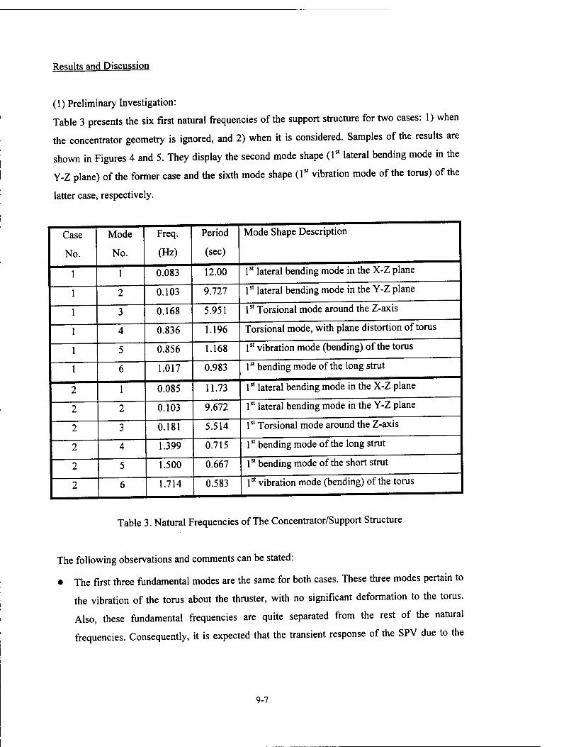
Results and Discussion
(1) Preliminary Investigation:
Table 3 presents the six first natural frequencies of the support structure for two cases: 1) when
the concentrator geometry is ignored, and 2) when it is considered. Samples of the results are
shown in Figures 4 and 5. They display the second mode shape (1st lateral bending mode in the
Y-Z plane) of the former case and the sixth mode shape (1st vibration mode of the torus) of the
latter case, respectively.
Case
No.
Mode
No.
Freq.
(Hz)
Period
(sec)
Mode Shape Description
1 0.083 12.00 1st lateral bending mode in the X-Z plane
2 0.103 9.727 1st lateral bending mode in the Y-Z plane
3 0.168 5.951 1st Torsional mode around the Z-axis
4 0.836 1.196 Torsional mode, with plane distortion of torus
5 0.856 1.168 1st vibration mode (bending) of the torus
6 1.017 0.983 1st bending mode of the long strut
2 1 0.085 11.73 1st lateral bending mode in the X-Z plane
2 2 0.103 9.672 1st lateral bending mode in the Y-Z plane
2 3 0.181 5.514 1st Torsional mode around the Z-axis
2 4 1.399 0.715 1st bending mode of the long strut
2 5 1.500 0.667 1st bending mode of the short strut
2 6 1.714 0.583 1st vibration mode (bending) of the torus 1
Table 3. Natural Frequencies of The Concentrator/Support Structure
The following observations and comments can be stated:
• The first three fundamental modes are the same for both cases. These three modes pertain to
the vibration of the torus about the thruster, with no significant deformation to the torus.
Also, these fundamental frequencies are quite separated from the rest of the natural
frequencies. Consequently, it is expected that the transient response of the SPV due to the
9-7
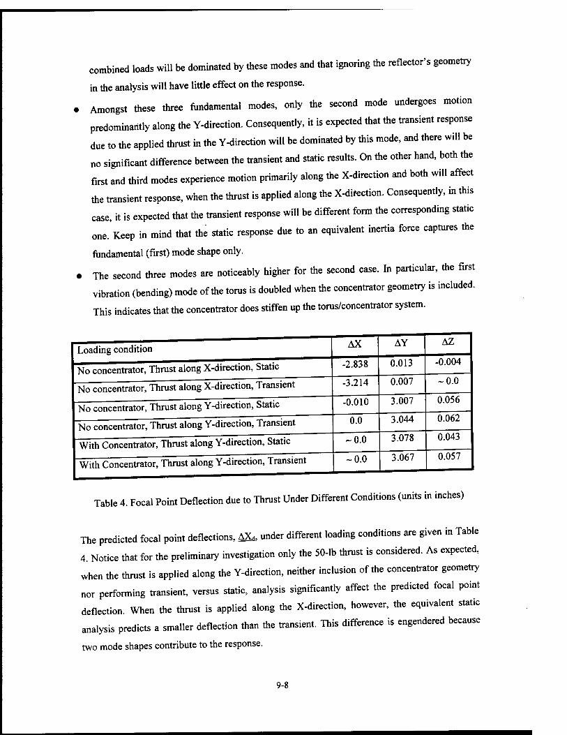
combined loads will be dominated by these modes and that ignoring the reflector's geometry
in the analysis will have little effect on the response.
Amongst these three fundamental modes, only the second mode undergoes motion
predominantly along the Y-direction. Consequently, it is expected that the transient response
due to the applied thrust in the Y-direction will be dominated by this mode, and there will be
no significant difference between the transient and static results. On the other hand, both the
first and third modes experience motion primarily along the X-direction and both will affect
the transient response, when the thrust is applied along the X-difection. Consequently, in this
case, it is expected that the transient response will be different form the corresponding static
one. Keep in mind that the static response due to an equivalent inertia force captures the
fundamental (first) mode shape only.
The second three modes are noticeably higher for the second case. In particular, the first
vibration (bending) mode of the torus is doubled when the concentrator geometry is included.
This indicates that the concentrator does stiffen up the torus/concentrator system.
Loading condition
No concentrator, Thrust along X-direction, Static
No concentrator, Thrust along X-direction, Transient
No concentrator, Thrust along Y-direction, Static
No concentrator, Thrust along Y-direction, Transient
AX
-2.838
-3.214
-0.010
With Concentrator, Thrust along Y-direction, Static
With Concentrator, Thrust along Y-direction, Transient
0.0
AY
0.013
0.007
3.007
3.044
-0.0
0.0
3.078
3.067
AZ
-0.004
0.0
0.056
0.062
0.043
0.057
Table 4. Focal Point Deflection due to Thrust Under Different Conditions (units in inches)
The predicted focal point deflections, AX*, under different loading conditions are given in Table
4. Notice that for the preliminary investigation only the 50-lb thrust is considered. As expected,
when the thrust is applied along the Y-direction, neither inclusion of the concentrator geometry
nor performing transient, versus static, analysis significantly affect the predicted focal point
deflection. When the thrust is applied along the X-direction, however, the equivalent static
analysis predicts a smaller deflection than the transient. This difference is engendered because
two mode shapes contribute to the response.
9-8
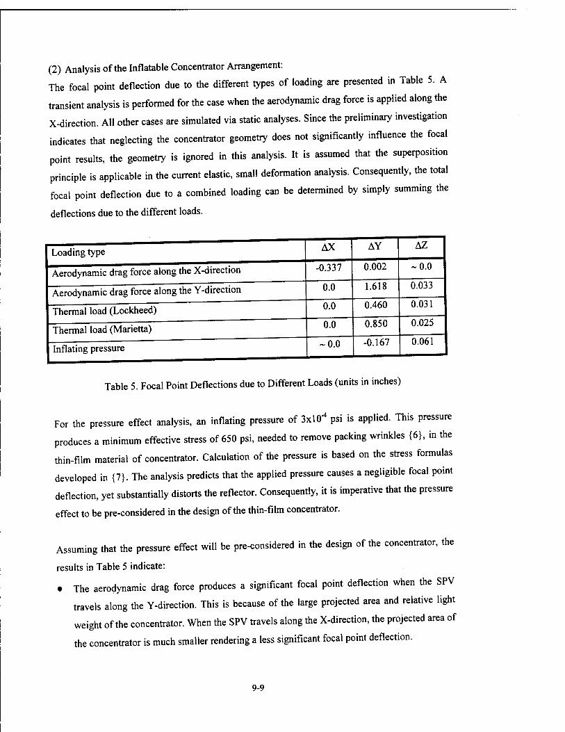
(2) Analysis of the Inflatable Concentrator Arrangement:
The focal point deflection due to the different types of loading are presented in Table 5. A
transient analysis is performed for the case when the aerodynamic drag force is applied along the
X-direction. All other cases are simulated via static analyses. Since the preliminary investigation
indicates that neglecting the concentrator geometry does not significantly influence the focal
point results, the geometry is ignored in this analysis. It is assumed that the superposition
principle is applicable in the current elastic, small deformation analysis. Consequently, the total
focal point deflection due to a combined loading can be determined by simply summing the
deflections due to the different loads.
Loading type AX AY AZ
Aerodynamic drag force along the X-direction -0.337 0.002 -0.0
Aerodynamic drag force along the Y-direction 0.0 1.618 0.033
Thermal load (Lockheed) 0.0 0.460 0.031
Thermal load (Marietta) 0.0 0.850 0.025
Inflating pressure -0.0 -0.167 0.061
Table 5. Focal Point Deflections due to Different Loads (units in inches)
For the pressure effect analysis, an inflating pressure of 3X10"4 psi is applied. This pressure
produces a minimum effective stress of 650 psi, needed to remove packing wrinkles {6}, in the
thin-film material of concentrator. Calculation of the pressure is based on the stress formulas
developed in {7}. The analysis predicts that the applied pressure causes a negligible focal point
deflection, yet substantially distorts the reflector. Consequently, it is imperative that the pressure
effect to be pre-considered in the design of the thin-film concentrator.
Assuming that the pressure effect will be pre-considered in the design of the concentrator, the
results in Table 5 indicate:
• The aerodynamic drag force produces a significant focal point deflection when the SPV
travels along the Y-direction. This is because of the large projected area and relative light
weight of the concentrator. When the SPV travels along the X-direction, the projected area of
the concentrator is much smaller rendering a less significant focal point deflection.
9-9
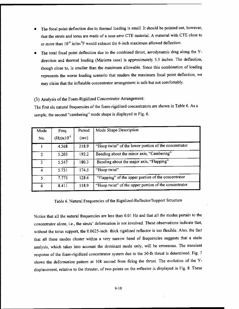
• The focal point deflection due to thermal loading is small. It should be pointed out, however,
that the struts and torus are made of a near-zero CTE material. A material with CTE close to
or more than 10"6 in/in-°F would exhaust the 6-inch maximum allowed deflection.
• The total focal point deflection due to the combined thrust, aerodynamic drag along the Y-
direction and thermal loading (Marietta case) is approximately 5.5 inches. The deflection,
though close to, is smaller than the maximum allowable. Since this combination of loading
represents the worse loading scenario that renders the maximum focal point deflection, we
may claim that the inflatable concentrator arrangement is safe but not comfortably.
(3) Analysis of the Foam-Rigidized Concentrator Arrangement:
The first six natural frequencies of the foam-rigidized concentrators are shown in Table 6. As a
sample, the second "cambering" mode shape is displayed in Fig. 6.
Mode
No.
Freq.
(Hz)xl(T
4.568
5.203
5.547
5.731
7.773
8.411
Period
(sec)
218.9
192.2
180.3
174.5
128.6
118.9
Mode Shape Description
'Hoop twist" of the lower portion of the concentrator
Bending about the minor axis, "Cambering"
Bending about the major axis, "Flapping"
'Hoop twist"
"Flapping" of the upper portion of the concentrator
'Hoop twist" of the upper portion of the concentrator
Table 6. Natural Frequencies of the Rigidized-Reflector/Support Structure
Notice that all the natural frequencies are less than 0.01 Hz and that all the modes pertain to the
concentrator alone, i.e., the struts' deformation is not involved. These observations indicate that,
without the torus support, the 0.0625-inch thick rigidized reflector is too flexible. Also, the fact
that all these modes cluster within a very narrow band of frequencies suggests that a static
analysis, which takes into account the dominant mode only, will be erroneous. The transient
response of the foam-rigidized concentrator system due to the 50-lb thrust is determined. Fig. 7
shows the deformation pattern at 108 second from firing the thrust. The evolution of the Y-
displacement, relative to the thruster, of two points on the reflector is displayed in Fig. 8. These
9-10
two points are the connection points between the reflector and the long strut (UYRL), and
between the reflector and the short strut (UYRS). Notice the prohibitively large displacement and
severe distortion experienced by the reflector. Obviously, the rigidized-concentrator is too
flexible to preserve its geometric integrity against the inertial effect of the applied thrust.
Conclusion
A finite element investigation of the SPV with the 1574.8x1181.1 inches off-axis parabolic
concentrator is conducted. Two concentrator arrangements are examined: inflatable thin-film
concentrator with a support torus and a foam rigidized-concentrator without the torus. The
combined effect of the thrust, aerodynamic drag, and thermally-induced deformation on the focal
point accuracy is assessed. Presuming that the struts and tori are made of a near-zero CTE
material and that the pressure effects on the reflector is pre-considered, the inflatable thin-film
concentrator fulfills the required accuracy of the focal point deflection. The foam-rigidized
concentrator, on the other hand, severely fails to satisfy this required accuracy.
The above-mentioned conclusions suggest that a combination of both arrangements would be the
most effective. A vehicle with a rigidized concentrator and a smaller torus would have sufficient
stiffness to comfortably achieve the needed focal point accuracy. In addition, this arrangement
will purge the vehicle from the canopy. Thereby, it will improve the optical quality of the
reflector and overcome the problems associated with maintaining the inflation of the
concentrator. More over, in order to further reduce the focal point deflection, adding some
damping to the support structure is recommended. This damping will also attenuate the
developed oscillatory motion and prevent multiplication of this oscillation upon repeated firing.
Since the inflatable concentrator arrangement already satisfies the required deflection point
accuracy, passive damping is considered adequate for this support structure. The constrained
layer damping {8}, shunted piezoelectric {9}, and electromechanical surface damping {10} are
passive, economical and reliable techniques that we recommend to be considered for this
application.
9-11

References
1. K.K. Laug, "The Solar Propulsion Concept is Alive and Well at the Astronautics
Laboratory," 1989 JANNAF Propulsion Meeting, 23-25 May 1989, CPIA Publication 515,
Vol. 1, pp. 289-324.
2. G.L. Ritchie, D.M. Chisessi, and J.F. Wilson, "Solar Astromast Torus," Final Report No.
AFRPL-TR-93-3034, Lockheed Missiles and Space Company, August 1993.
3. J. Paxton, and C. Hawk, "Material Property Effects on a Thin Solar Concentrator for Solar
Thermal Propulsion," 30th AIAA/ASME/SAE/ASEE Joint Propulsion Conference,
1994/Indianapolis, IN, AIAA Publication 94-3029, 1994, pp. 1-12.
4. J.L. Draper, R.N. Gehling, R.R. Hanson, D.F. Shepard, and J.L. Summers,
"Graphite/Kelvar™ Strings Truss," Final Report No. AFRPL-TR-93-3032, Martin Marietta
Astronautics Group, September 1993.
5. M.R. Holmes, "Ideal Performance of Off-Axis Paraboloid Concentrators for Solar-Thermal
Propulsion," The 1996 International Solar Energy Conference, ASME Puplication, edit. J.H.
Davidson, 1996, pp. 443-449.
6. G.R. Veal, "Highly Accurate Inflatable Reflectors, Phase II," L'Garde, Inc. Final Report No.
AFRPL-TR-86-089, March 1987.
7. G. Grossman, "Analysis of Rim Supports for Off-Axis Inflatable Reflectors. I: Loads,"
Journal of Aerospace Engineering, Vol. 4, 1991, pp.47-66.
8. G.R. Tomlinson, "The use of Constrained Layer Damping in Vibration Control,"
International Journal of Mechanics and Sciences, Vol. 32, 1990, pp. 233-242.
9. N.W. Hagood, and A. von Flotow, "Damping of Structural Vibrations With Piezoelectric
Materials and Passive Electrical Networks," Journal of Sound and Vibration, Vol. 146, 1991,
pp. 243-268.
10. H. Ghoneim, "Application of the Electromechanical Surface Damping to the Vibration
Control of a Cantilever Plate," ASME Journal of Vibration and Acoustics, Vol. 118, 1996,
pp. 551-557.
9-12
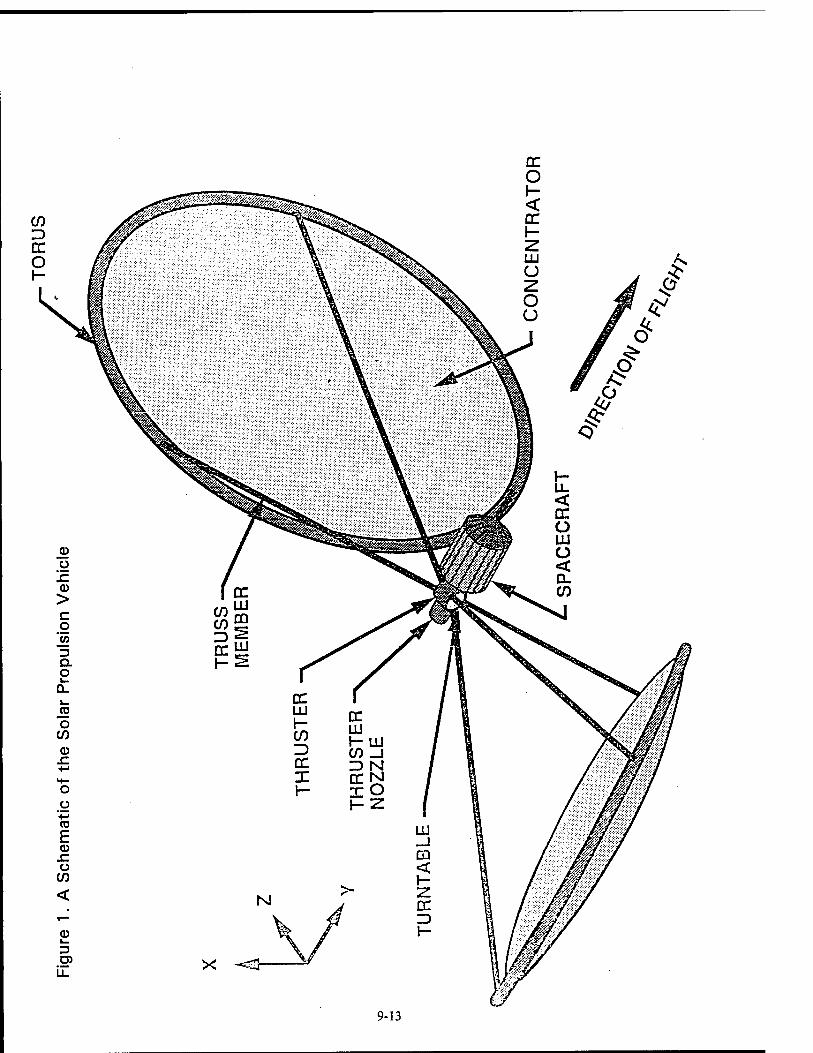
9-13
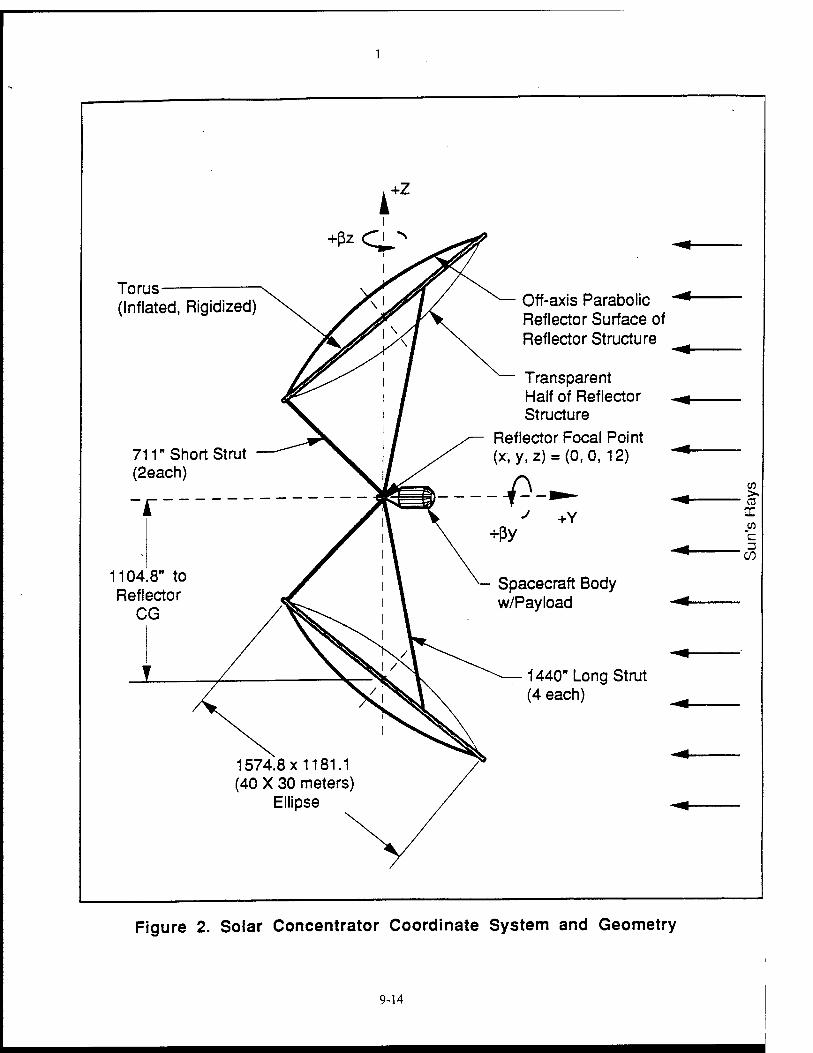
Torus (Inflated, Rigidized)
711" Short Strut (2each)
1104.8" to Reflector
CG
1574.8x1181.1 (40 X 30 meters)
Ellipse
Off-axis Parabolic Reflector Surface of Reflector Structure
Transparent Half of Reflector Structure
Reflector Focal Point (x, y, z) = (0, 0, 12)
-—A- +Y
Spacecraft Body w/Payload
1440" Long Strut (4 each)
>. ' 03
c D
'00
Figure 2. Solar Concentrator Coordinate System and Geometry
9-14
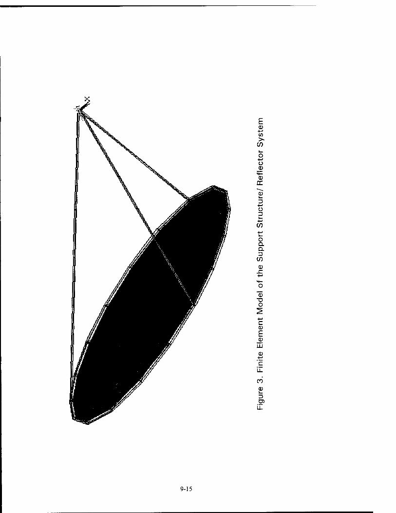
E Q)
w >
CO
o o
DC
ID I_ D
■M o 3 i—
■4->
CO
o a a CO 0 x:
0 ■o o
c a) E
LU
0
CO
Q)
9-15
.J.. ..X
/ / /
( I I / i / I / \ / \ / \ ■•
V
1 \ ■^ - - \
~~~~~~~-X''
\ v. \ '-; \ \ ;- \ "\ .\ \ \ \ \ \ \ | \ 1 \ \ \ / \ / \ / \J
XLJ^JJHT'
Figure 4. Second Mode Shape of the Inflatable Concentrator/Support Structure With the Concentrator's Geometry Ignored
(Dashed Line Represents the Undeformed Shape)
9-16
Figure 5. Sixth Mode Shape of the inflatable Concentrator/Support Structure (Dashed Line Represents the Undeformed Shape)
9-17
Figure 6. Second Mode Shape of the Foam-Rigidized Concentrator/Support Structure
(Dashed Line Represents the Undeformed Shape)
9-18
Figure 7. Deformed Shape of the Foam-Rigidized concentrator due to a 50-lb Thrust Acting Along the Y-Direction (at 108 Second)
9-19
ÜYRS
CO CD
SI ü c
c o ü
CD Q
Time (Second)
Figure 8. Evolution of the Relative Y-Deflection due to the 50-lb Thrust (UYRL = The Connection Point Between the Reflector and Long Strut, UYRS = The Connection Point Between the Reflector and Short Strut)
9-20
DESIGNING PROPULSION REALIABILITY OF SPACE LAUNCH VEHICLES
Subir Ghosh Associate Professor
Department of Statistical Engineering
University of California Riverside, CA 92521
Final Report for: Summer Research Program
Phillips Laboratory
Sponsored by: Air Force Office of Scientific Research
Boiling Air Force Base, Washington, DC
And
Phillips Laboratory
September, 1997
10-1
DESIGNING PROPULSION RELIABILITY
OF SPACE LAUNCH VEHICLES
Subir Ghosh
Professor
Department of Statistics
University of California, Riverside
Abstract
The propulsion reliability of a thrust-augmented Single Stage to Orbit (SSTO) space
launch vehicle depends on the number of solid boosters, the number of liquid engines, the
reliability per solid booster, and the reliability per liquid engine. We give mathematical
expressions of such dependence when the reliability does or does not depend on time.
We present numerical results and corresponding figures demonstrating the relationship
between the propulsion cluster reliability and the motor/engine reliabilities of both solid
booster and liquid engines. This paper shows how the propulsion cluster reliability can be
tailored to match a desired vehicle reliability.
10-2

DESIGNING PROPULSION RELIABILITY
OF SPACE LAUNCH VEHICLES
Subir Ghosh
Introduction
Single Stage to Orbit (SSTO) launch vehicle reliability is an important part of the
performance evaluation of this class of vehicles. Our research is concerned with the
propulsion reliabilities of space vehicles for catastrophic failures. Four methods are
developed for calculating the propulsion reliability of such a vehicle. Launch vehicles with
different combinations of solid booster and liquid engines are considered. The dependence
of the propulsion cluster reliability on the numbers of solid boosters and liquid engines is
studied. Specific recommendations are made for designing an SSTO vehicle with respect
to the desired solid booster and liquid engines reliabilities as well as the cluster propulsion
reliability of the vehicle. Historical data are used for defining representative reliabilities.
A literature search does not find much published work available on vehicle reliability
formulation. The work presented here presents new thinking in vehicle design.
Propulsion Reliability Models: Blocked Series System
In a blocked series system, solid boosters and liquid engines are considered as two blocks
with series system in each. We first present the formula for calculating the non-time
dependent propulsion reliability of an SSTO. Let
Solid Booster
Number = »/
Reliability = pi
Series System
Liquid Engine
Number = «2
Reliability = P2
Series System
(1)
We assume that all solid boosters have the same reliability/?/ and all liquid engines have
the same reliability^. The failures of propulsion, solid or liquid, are assumed to be
independent and furthermore, a failure of any propulsion unit, solid or liquid, results in the
10-3
catastrophic failure of the propulsion system and consequently, the catastrophic failure of
the space vehicle. This is known as a series system for both solid boosters and liquid
engines. The probabilistic setup is called a Binomial Experiment. The non-time
dependent cluster reliability/?/ of the space vehicle can be expressed as
*i = 1-K0- />,"') +Mi-/>;■)]■ (2)
Note that we want 0 < Rj < 1, which in turn sets constraints on «/, pi, »2andp2 for
reasonable values.
We now present the formula for calculating the time dependent propulsion
reliability of an SSTO. We assume an Exponential Model with
(-r/0,) px = e ,0 < t < 90,
i-t/02) p2 = e ,0 < t < 500, (3)
where 0/ and 92 are unknown parameters. Note that the expressions of pi and p2 given in
(3) are time dependent. The operation time of solid boosters is assumed to be the first 90
seconds and the operation time of liquid engines is assumed to be the period of 500
seconds. The time dependent cluster reliability R2 of the space vehicle can be expressed as
R2 = l-[«1{l-(e(-'/<?'))"'} + «2{l-(e(-'/^))"J}],0 < / < 90,
R2 = l-[«2{l-(e(-'/Ö2))"2}],90 < / <500. (4)
Non-Time Dependent Reliability : Blocked Series System
In this section, we study the dependence of Ri, defined in (2), on W/ and «2. Table 1
presents the overall reliability ( Ri ) values for/?/ = 0.9999 andp2 = 0.9990 and 0.9999,
Table 2 presents the R} values for/?/ = 0.999 mdp2 = 0.992 and 0.999. Figures 1.1 and
10-4
1.2 display R, curves for ( n,,n2) = ( 0, 2), (2, 4 ), ( 3, 6 ) and/?; = 0.9999 and 0.999,
respectively.
•Solid = 0 Liquid = 2
»Solid = 2 Liquid = 4
•Solid = 3 Liquid = 6
0.992 0.994 0.996 Liquid Engine Reliability
Figure 1.1 : Propulsion Reliability by Liquid Engine Reliability when Solid Booster Reliability = 0.999 : Blocked Series
'Solid = 0 Liquid = 2
•Solid = 2 Liquid = 4
•Solid = 3 Liquid =6
0.9992 0.9994 0.! Liquid Engine Reliability
0.9998
Figure 1.2 : Propulsion Reliability by Liquid Engine Reliability when Solid Booster Reliability = 0.9999 : Blocked Series
Figures 2.1 - 2.4 display contour plots of Ri values. These graphs are useful for the
purpose of reliability design. For designing a space vehicle with/?/ = 0.9999 and/??
= 0.9999, the problem is to find the values of«/ and n2 so that the desired propulsion
reliability R, is 0.999. The possible values of (n,, n2) are ( 2, 2 ), ( 2, 3 ), ( 1, 2 ),
( 1, 3 ), (0, 2 ). Considering the desired performance and cost analyses, one could
come up with the optimum choice of (w/, n2). If the desired propulsion reliability
10-5
1 2
Number of Solid Boosters
Figure 2.1: Propulsion Reliability Contour: Solid = 0.9999, Liquid = 0.9999 Blocked Series
° 0.968
0.976
0.984
3 0.992
1 ~ 1 2
Number of Solid Boosters
Figure 2.2 : Propulsion Reliability Contour: Solid = 0.9999, Liquid = 0.999 Blocked Series
10-6
Number of Solid Boosters
Figure 2.3 : Propulsion Reliability Contour: Solid = 0.999, Liquid = 0.999 Blocked Series
0.749
0.798
0.847
0.896
1 2 Number of Solid Boosters
Figure 2.4 : Propulsion Reliability Contour : Solid = 0.999, Liquid = 0.992 Blocked Series
10-7
Table 1. Non-Time Dependent Propulsion Reliability, R, .when/;, = 0.9999,p2 = 0.9990 and 0.9999
p2 = 0.9990
3
n2 2 0.9960 0.9959 0.9956 0.9951
0.9901
0.9831
0.9742
0.9632
0
2 0.9960
3 0.9910
4 0.9840
5 0.9751
6 0.9641
"i
0
2 0.9996
3 0.9991
4 0.9984
5 0.9975
6 0.9964
1 2
0.9959 0.9956
0.9909 0.9906
0.9839 0.9836
0.9750 0.9747
0.9640 0.9637
P2 = 0.9999
1 2
0.9995 0.9992
0.9990 0.9987
0.9983 0.9980
0.9974 0.9971
0.9963 0.9960
3
n2 2 0.9996 0.9995 0.9992 0.9987
0.9982
0.9975
0.9966
0.9955
Tables 2. Non-Time Dependent Propulsion Reliability, Ru when/», = 0.999 , and/;; = 0.992 and 0.999
p2 = 0.992
3
n2 2 0.9681 0.9671 0.9641 0.9591
0.9196
0.8645
0.7942
0.7087
»i
0
2 0.9681
3 0.9286
4 0.8735
5 0.8032
6 0.7177
";
0
2 0.9960
3 0.9910
4 0.9840
5 0.9751
6 0.9641
1 2
0.9671 0.9641
0.9276 0.9246
0.8725 0.8695
0.8022 0.7992
0.7167 0.7137
p2 = 0.999
1 2
0.9950 0.9920
0.9900 0.9870
0.9830 0.9800
0.9741 0.9711
0.9631 0.9601
3
n2 2 0.9960 0.9950 0.9920 0.9870
0.9820
0.9750
0.9661
0.9551
10-8

Rj is 0.995 ( one catastrophic failure in 200 attempts ), then with (w/ = 2, n2 =4), we need
p2 = 0.9997 for/?; = 0.9999 as it can be seen from Figure 1.1. Similarly with
(nj = 3, n2 = 6), we need/?2= 0.9999 for/?7= 0.9999. However, with neither
(/?/ = 2, n2 = 4) nor (w/ = 3, n2 = 6), we can achieve the cluster reliability Ri = 0.995
for pi = 0.999. This can be done for (n, = 0, n2 = 2) withp2 = 0.999. For an
experimental SSTO with 1/200 catastrophic failure rate, a propulsion cluster of
two liquid engines with each of 0.999 reliability is required. More liquid engines or
strap-on solid boosters lower the overall vehicle reliability. Current Space Shuttle Main
Engines ( SSME) have demonstrated close to 0.999 reliability after approximately 2,000
full-duration tests since 1979 ( Biggs (1997)).
Time Dependent Reliability : Blocked Series System
We now study the dependence of R2, defined in (4), on /,«/, and n2. For ri] = 1, 2, and n2
= 2, 3, 4, we determine 0, and ft so that R2= 0.995 for t = 90 sec and / = 500 sec. For «y
= 0 and n2 = 2,3,4, we find ft so that R2 = 0.995 for t = 500 sec. As a result, with our
determined values of 6, and 02, R2 > 0.995 for 0 < / < 500. Figures 3.1-3.3 demonstrate
the change in the cluster reliability R2 with time t for W/ = 0, 1, and 2. For n, = 2, we
observe that after 90 sec theR2 values stay at 0.995. For n} = \,R2= 0.995 at / = 90
sec, jumps to R2 = 0.999 at / = 91 sec, and finally becomes R2 = 0.995 at t = 500 sec. For
«/ = 0, R2 decreases from 1 to 0.995 for t = 0 sec to / = 500 sec. Figures 4.1 - 4.3 display
the change in reliability per liquid engine over time for 2, 3, and 4 liquid engine vehicles.
In order to achieve the cluster reliability of at least 0.995 during the 500 sec, the reliability
per liquid engine drops to 0.998751 for a 2 liquid engines vehicle compared to 0.999687
for a 4 liquid engines vehicle with 2 solid boosters for both. For a vehicle with nt = 2, n2
= 2, the reliability per liquid engine at 500 sec is 0.99875. If we calculate the cluster
reliability at 500 sec by (0.99875 f, we get 0.997502 which is much higher than 0.995
obtained from the time-dependent exponential model.
10-9
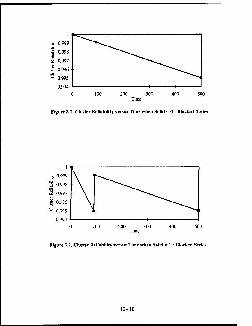
100 200 300 Time
400 500
Figure 3.1. Cluster Reliability versus Time when Solid = 0 : Blocked Series
100 200 . 300 Time
400 500
Figure 3.2. Cluster Reliability versus Time when Solid = 1: Blocked Series
10-10
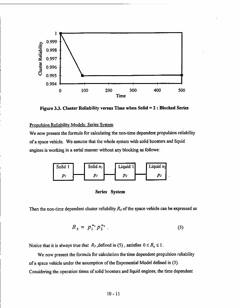
>, 0.999 -
0 100 200 300 Time
400 500
Figure 3.3. Cluster Reliability versus Time when Solid = 2 : Blocked Series
Propulsion Reliability Models: Series System
We now present the formula for calculating the non-time dependent propulsion reliability
of a space vehicle. We assume that the whole system with solid boosters and liquid
engines is working in a serial manner without any blocking as follows:
Solid 1
Pi
Solid rii
Pi
Liquid 1
P2
Liquid «;
P2
Serii es Sy stem
Then the non-time dependent cluster reliability R3 of the space vehicle can be expressed as
*3 = PVP? . (5)
Notice that it is always true that R3 .defined in (5), satisfies 0 < R3 < 1.
We now present the formula for calculation the time dependent propulsion reliability
of a space vehicle under the assumption of the Exponential Model defined in (3).
Considering the operation times of solid boosters and liquid engines, the time dependent
10-11
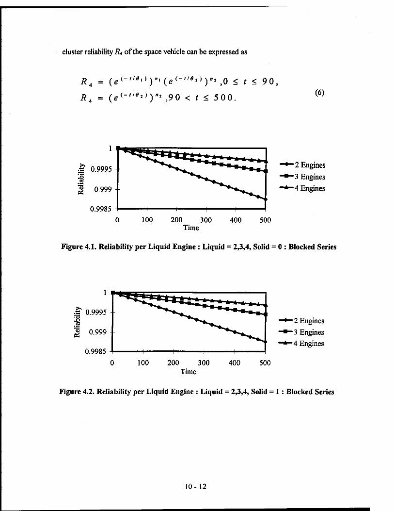
cluster reliability R4 of the space vehicle can be expressed as
R4 = (^-'"'))»'(g<-'"»))«»)0 < t < 90
R4 = (e(-"*»>)»* ,90 < t < 500. (6)
0
•2 Engines
•3 Engines
•4 Engines
100 200 300 Time
400 500
Figure 4.1. Reliability per Liquid Engine : Liquid = 2,3,4, Solid = 0 : Blocked Series
£ 0.9995
100 200 300 Time
"2 Engines
■3 Engines
'4 Engines
400 500
Figure 4.2. Reliability per Liquid Engine : Liquid = 2,3,4, Solid = 1 : Blocked Series
10-12
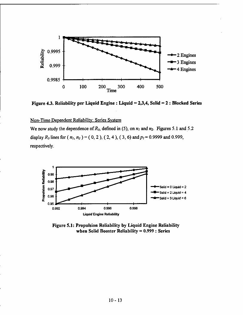
£ 0.9995
•8 p§ 0.999 - -
-^2 Engines ^*-3 Engines -^-4 Engines
200 300 Time
500
Figure 4.3. Reliability per Liquid Engine : Liquid = 2,3,4, Solid = 2 : Blocked Series
Non-Time Dependent Reliability: Series System
We now study the dependence ofR3, defined in (5), on «/ and n2. Figures 5.1 and 5.2
display R3 lines for (n,, n2) = ( 0, 2), ( 2, 4 ), ( 3, 6) and/?/ = 0.9999 and 0.999,
respectively.
'Solid = 0 Liquid = 2
'Solid = 2 Liquid = 4
'Solid = 3 Liquid = 6
0.994 0.996
Liquid Engine Reliability
0.998
Figure 5.1: Propulsion Reliability by Liquid Engine Reliability when Solid Booster Reliability = 0.999 : Series
10-13
■Solid = 0 Liquid = 2
-Solid = 2 Uquid = 4
•Solid = 3 Liquid = 6
0.9992 0.9994 0.9996
Liquid Engine Reliability
0.9998
Figure 5.2 : Propulsion Reliability by Liquid Engine Reliability when Solid Booster Reliability = 0.9999 : Series
Figures 6.1 - 6.4 display contour plots of R3 values. We observe that the contour plots of
R3 for Methods 1 and 2 are different when/?/ =p2 as can be seen in Figures 2.1 and 6.1 as
well as in Figures 2.3 and 6.3. However, the contour plots of R3 for Methods 1 and 2
are very similar when/»/ andp2 differ widely as can be seen in Figures 2.2 and 6.2 as well
as in Figures 2.4 and 6.4.
1 2
Number of Solid Boosters
Figure 6.1. Propulsion Reliability Contour: Solid = 0.9999, Liquid = 0.9999 : Series
10-14
N:
1 2 Number of Solid Boosters
Figure 6.2. Propulsion Reliability Contour: Solid = 0.9999, Liquid = 0.999 : Series
1 2 Number of Solid Boosters
Figure 6.3. Propulsion Reliability Contour: Solid = 0.999, Liquid = 0.999 : Series
10-15
-öS«
0.960
0.966 "
4"
3-
l
Number of Solid Boosters
Figure 6.4. Propulsion Reliability Contour: Solid = 0.999, Liquid = 0.992 : Series
Time Dependent Reliability: Series System
We now study the dependence of R4, defined in (6), on t, nIt and n2. Figures 7.1- 7.3
show the change in the cluster reliability R4 with time t for rij = 0, 1, and 2. The
comparison of R4 values from Methods 1 and 2 can be made from Figures 3.1-3.3 and
Figures 7.1-7.3. The R4 values are very similar except for /?/ = 2 as can be seen from
Figures 3.3 and 7.3. In Method 1, the R, values stay at 0.995 for w; = 2 for t > 90 but ,in
Method 2, the R4 value jumps from 0.995 to 0.999 for / = 90 to the immediately higher t
and drops linearly to 0.995 at / = 500. Figures 8.1-8.3 display the change in reliability per
liquid engine, under Method 2, over time for 2,3, and 4 liquid engine vehicles. Methods 1
and 2 resemble each other with respect to the change in reliability per liquid engine as can
be seen from Figures 4.1-4.3 and 8.1-8.3.
10-16
1 )
0.999 -
§ 0.998 - 1 ••§ 0.997 - cd « 0.996 - 3 0 0.995 -
0.994 - 1 1 1 1
0 100 200 300 Time
400 500
Figure 7.1. Cluster Reliability versus Time when Solid = 0 : Series
100 200 300
Time
400 500
Figure 7.2. Cluster Reliability versus Time when Solid = 1: Series
10-17
11
0.999
§ 0.998 •8 'S 0.997 Pi
2 0.996 + Ui 3 Ö 0.995
0.994
0 100 200 300
Time
400 500
Figure 7.3. Ouster Reliability versus Time when Solid = 2 : Series
500
•2 Engines •3 Engines '4 Engines
Figure 8.1. Reliability per Liquid Engine : Liquid = 2,3,4, Solid = 0 : Series
Conclusions
This study is on the propulsion reliability (R) of an SSTO vehicle as a function of the
number of solid boosters ( «/ ), the reliability per solid booster (pi ), the number of liquid
engines ( W;), and the reliability per liquid engines (p2). Both time dependent and non-
time dependent models are considered for/?/ and/?2 . Two models ,series and blocked
series, are considered for R . Our findings for non-time dependent
10-18
1
0.9995 -
g 0.999
1 0.9985
0.998 3 0.9975
0.997 -I
0 100 200 300
Time
400 500
•2 Engines
• 3 Engines
•4 Engines
Figure 8.2. Reliability per Liquid Engine : Liquid = 2,3,4, Solid = 1: Series
1
0.9995
£• 0.999 +
■S 0.9985
0.998 + £ 0.9975
0.997
100 200 300
Time
400 500
• 2 Engines
• 3 Engines
•4 Engines
Figure 8.3. Reliability per Liquid Engine : Liquid = 2,3,4, Solid = 2 : Series
blocked series reliability model with R > 0.995 are summerized in Table 3. Table 3
describes the number of solid boosters and liquid engines to choose for targetting
the propulsion reliability at 0.995. The number of liquid engines is recommended to be
two or three and the number of solid boosters is recommended to zero or one if their
reliabilities are in between 0.9990 and 0.9995. In order to have more solid boosters and
liquid engines with the same desired propulsion reliability 0.995, we need their reliabilities
to be higher than 0.9995. Our findings for series model are similar to block series model.
For the time dependent model, the propulsion cluster reliability drops rapidly over time in
10-19
P2 «7
Liquid Solid
0.9990 0,1 0.9995 0
1 0.9999 0,1
2 0.9990 0,1 0.9995 0,1
2 0.9999 0,1
2 3
0.9990 0,1,2,3 0.9995 0,1,2
3
presence of solid boosters but then after 90 seconds it jumps higher and decays at a much
slower rate or remains the same. Moreover, for maintaining the propulsion reliability at
0.995 or higher over 500 seconds, the reliability per liquid engine drops more rapidly over
time for four liquid engines than two or three liquid engines.
Table 3. Solutions for »j and n2 to have at least 0.995 for R in the non-time dependent case
Model pi P2 ni n2 Solid Liquid Solid Liquid
Blocked Series 0.9990 0.9990 0,1 2 2,3 2 2,3,4,5,6 2,3
0.9995 0.9990 0,1 2 2,3 2 2,3,4,5,6 2,3,4,5 2
0.9999 0.9990 0,1,2,3 2 2,3 2
0.9999 0,1,2,3 2,3,4,5,6 Acknowledgments
I would like to thank Terence Galati for the valuable discussions, guidance, and
information. I am grateful to Francis McDougall for all his help and kindness. My sincere
thanks also to Dr. Ray Moszee and to the Air Force Office of Scientific Research for
making this possible.
References
Biggs, B. ( 1997 ). SSME Flight Reliability Determination. Rocketdyne.
Elsayed, E. A. (1996). Reliability Engineering. Addison Wesley Longman, Inc.,
Massachusetts.
Lloyd, D. K., and Lipow, M. ( 1984). Reliability: Management, Methods, and
Mathematics. The American Society for Quality Control, Milwaukee,
Wisconsin.
Report of the Presidential Commision on the Space Shuttle Challenger Accident.
(1986): Prepared by W. P. Rogers et al., Washington, D. C.
10-20
ASYMPTOTIC ANALYSIS OF THE NATURAL SYSTEM MODES OF COUPLED BODIES IN THE LARGE
SEPARATION, LOW-FREQUENCY REGIME
George W. Hanson Associate Professor
Department of Electrical Engineering and Computer Science
University of Wisconsin-Milwaukee 3200 N. Cramer Street
Milwaukee, Wisconsin 53211
Final Report for: Summer Faculty Research Program
Phillips Laboratory
Sponsored by: Air Force Office of Scientific Research
Boiling Air Force Base, DC
and
Phillips Laboratory
July 1997
ll-l
ASYMPTOTIC ANALYSIS OF THE NATURAL SYSTEM MODES OF COUPLED BODIES IN THE LARGE
SEPARATION, LOW-FREQUENCY REGIME
George W. Hanson Associate Professor
Department of Electrical Engineering and Computer Science University of Wisconsin-Milwaukee
Abstract
In this report we examine the natural electromagnetic system modes (characteristic
frequencies and currents) of two coupled bodies in the limit of large separation. It is known that
when objects are situated such that they may interact electromagnetically, natural modes of the
coupled system occur. These modes differ from the natural modes of the isolated bodies, but
may be related to the isolated body modes for some situations. Here we treat an N-body
scattering problem in the limit of large separation by replacing the bodies with equivalent dipole
moments. The natural frequencies are obtained as singular points in the scattering solution. For
the special case of two coupled objects, a simple equation for the natural system frequencies is
obtained which shows that the real radian system frequency approaches the origin as l/r,
independent of the relative orientation and type of the two bodies. The damping coefficient
approaches the origin approximately logarithmically, as a function of the body orientation and
type. This simple equation leads to classification and ordering of some system modes based on
their behavior in the limit of large separation. Using this formulation, the natural system modes
of two coupled wires are investigated for large separation between the wires, and compared to
an integral equation solution.
11-2
ASYMPTOTIC ANALYSIS OF THE NATURAL SYSTEM MODES OF COUPLED BODIES IN THE LARGE
SEPARATION, LOW-FREQUENCY REGIME
George W. Hanson
I. Introduction
The electromagnetic response of coupled bodies is of interest in many applications, including
target detection and identification. In this note we consider the frequency (s-plane) behavior of the system
resonances of coupled objects in the limit of large separation.
In an early paper relating to the singularity expansion method (SEM) it was observed that the
SEM frequencies of an isolated thin wire scatterer can be grouped in layers in the s-plane nearly parallel
to the jo) axis [1]. These resonances are further identified by their position within these layers. This
observation naturally leads to the notation for the complex frequencies s°rl, where n denotes the nth
pole as measured from the Re(s) axis in the Jth layer, measured from the ja axis. Similar groupings
can be identified for other objects, but to illustrate the effect considered here the situation for thin wires
will be described. Shortly after the above observations were made concerning isolated wires, the natural system
frequencies of coupled wires were studied. It was found that these system resonances exhibited some
interesting characteristics as wire separation was varied [2]. To simplify the discussion, consider two
identical wires, for which the system resonances can be divided into symmetric (snstl) and antisymmetric
(saa#i) modes [14]. As observed in [2] for two thin wire scatterers, the low-order system resonances
(Sia,'iS) tended t0 sPiral around the dominant isolated body resonance (s°tl) as spacing between the
objects was varied over some intermediate distance. As separation was further increased, the system
resonances moved off towards the origin in the complex frequency plane, and other system modes from
another layer moved in to take their place, again spiraling around Sl°, x. Subsequent to [2], other papers
further considered coupled wire scatterers [3]-[4].
The fact that the system frequencies eventually tended towards the origin as spacing is increased
beyond some intermediate distance, rather than tending towards the isolated body resonances, was
discussed in [2], and explained from a time-domain perspective in [5]. It was observed that the SEM
system modes are global quantities for the coupled body system, and have no clear physical interpretation
11-3
prior to times when global modes can be established. Hence, in a two-body system the time period after
which the scattered field from each body has interacted with the other body is designated as late time.
During late time, the two objects interact electromagnetically, and global system modes are established.
As spacing between the objects becomes large relative to the largest linear dimension of each body, the
system resonances tend towards low frequencies since the time for a wave to travel between the two
bodies becomes long. Eventually the spacing tends towards infinity, and the system resonances tend
toward zero. Since the resonances of a coupled system are rigorously obtained from a complicated (usually
integral) system of equations, simple approximate formulas which describe the system resonance behavior
as a function of body separation are of interest. For intermediate separations, perturbation formulas have
been obtained which relate the natural system frequencies to the natural frequencies of the isolated bodies.
Two related classes of perturbation solution have been obtained, both based upon the exact integral-
operator description of the coupled system. The first method yields a quasi-analytic formula for the
system frequencies of an object and a mirror object, separated by some intermediate distance. The
resulting formula involves a numerically computed coefficient which only depends upon the isolated
object's characteristics, multiplied by an exponential term which is a function of the separation between
the objects [6]. The second method is more numerical in nature, yet represents a considerable
simplification of the exact IEs and is applicable to a more general system of coupled bodies [7]. The
formulation described in [7] was subsequently applied to a variety of coupled objects [5], [8]-[9].
In this note, we present a scattering formulation for N coupled objects valid in the limit of large
separation between all objects. The system of scatterers are replaced by interacting dipole moments,
which is a suitable approximation for large separations (which lead to low system frequencies). A simpler
formulation is provided for two objects coupled in a mirror symmetric configuration. Singularities of
the scattering solution are identified as natural frequencies, leading to the characteristic equation for
natural frequencies of the coupled system. The example of two coupled wires is considered to
demonstrate the accuracy of the asymptotic method, where the natural system frequencies from the
asymptotic formulation are compared to those generated from a full-wave integral equation solution. The
system modes are classified according to their behavior for large separation between the bodies, and some
results for the natural currents are provided to examine their behavior in the corresponding limit.
II. Preliminary Relations Consider Maxwell's curl equations for free space in the two-sided Laplace transform domain
11-4
Vx£(f, s) = -sB(f,s) -Jm{r, s) (1)
VxH(r,s) = sD(f,s) +Je(z,s) .
The relationships between fields and currents are given in terms of four Green's dyadics as [10]
E(f,s) =-s\L0{Geie(f\?/,s) ;Je(f',s))
\ e.n l (2)
H(ffs)=-se0{Ghtrn(f\f',s)iJm(f/,s)}
+(8hia(2\f,,s)i39(r,.8)}
where the bracket notation indicates a real inner product with integration over common spatial coordinates
(typically volume or surface integration). The Green's dyadics are
Ge Jf\f',s) =pv[l-y-2VV]G(f\f',s) +r2L(r)b(f-r') (3)
Geim{r\r',s) =-VG(f|f/,s)xl (4>
GhiB{2\T'.s)=-&9.m{2\2'.a) <5>
Ghtm(f\f',s)=Geie(f\f',s) <6>
where G{r\x',s) = ye~l is the free-space sealer Green's function, with Y = -§. S=Y*>
c= (€ |i ) ~1/2, and R = \ f - r' \. The first term in (3) can be written as
[i-Y-2vv]G(f|^S) = ^{[-2r3-2r2]i,i^[r3-r2-r1][i-^]} (7)
where i = f-f' , and 1 = lxlx + lyly + lzlz is the identity dyadic. For later convenience, define R \r-r'\'
11-5
yj? Fe,e(r\f',s) *-?—\[31RlR-l}
ATZ Ve0*
3 R2 + PÄ-q^°
(8)
with Z0=^ — , such that the Ge e term can be expressed as
Gp Ai\r',s) =PV—^Fe e(f\f',s) + y~2L(f) ö(f-f') . s2\i0 '
(9)
The magnetic Green's dyadic, Gem, can be expressed as
Geim{r\f',s) =-VG(r\r',s)xl = -^ 1 R2
s Re
lfixl
where upon defining for later convenience
FeJf\i',s) = „ . - e.m i ATC [ R2
£l!ff^£+ s2^°X
RC
(10)
(11)
the magnetic Green's dyadic can be written as
GeiJf\f',s) = -±-FeiJf\f>,s) lÄxl. (12)
In (3), the PV notation indicates that the corresponding term should be integrated in the principal value
sense [10], where
i r xs(f/) iR,{f\f_!lds> 4rc J \f-r'
(13)
is the depolarizing dyadic integral, evaluated over the surface 56 of the exclusion volume V6 excluded
in the PV integration. In(13), lR,{r\x') = -lR(f\f) =lR(r'\r) ,andls(f) is the unit normal
vector to S at f. Note that the G<e,e\ terms are properly interpreted as distributions. \h.ml
11-6
III. Scattering formulation
Consider a N-body scattering problem which can be analyzed by formulating a coupled set of
integral equations for the current (surface or volume polarization) induced on/in the objects by an incident
field. When the separation between all objects becomes large compared to the largest linear dimension
of each object, and in the limit of low frequency, the formulation can be considerably simplified by
replacing each object with equivalent dipole moments. This follows from the fact that the electric and
magnetic dipole moment terms dominant the fields due to a given current (as in a multipole expansion
of the current) for large distances and low frequencies [12]. To formulate the desired set of equations,
the scatterers, which are assumed to reside in free space, are replaced with dipole moments pp , 0
for ß = 1, 2, . . . , N corresponding to object 1,2,...N, respectively, as shown in Fig. 1. The dipoles
are considered to be generated by fields via polarizability dyadics as
p<P'(s) = e0P(P) (s)-E(?p,s)
p> (s) = M(p) {s)-H(fp.s)
(14)
fn^
where the fields {E, H) are the total fields due to all dipoles not located at fp, plus any externally
impressed field. The polarizability dyadics are symmetrical for reciprocal media,
P<p'r(s)=P(p)(s) (15)
M<p>r(s) =M(P) (S)
and as s-0 [12]
P(P)(s)=P0(P)+O(s) (i6)
The currents associated with the dipole moments are
JW-sßWö <*-.?,,) (17)
Jjp)=slJi02n(p)6(f-fp) .
Inserting (17) into (2) leads to the fields at fa maintained by electric and magnetic dipoles located atf p
as
11-7
£(a'P)(fa/s)=Fe/e(fB|fp,S)-p(P)(s)+Fe,m(fJfp,S) (l^xl)-Ä<l»(fl)
£(.,P> (fa#s) =_AFewn(fa|fp,S) (lÄo XiypW (8) +60Fe/e(fa|fp,S) •!'" (S)
(18)
where
^.a^J^'S* = >-t*:P
471 [31p 1R -ll
sZn
\eaRa,V Ra,pj
[-* -* **T *o Un 1R In "I ~
*«.» Ä«.P J Äaß
Fe.Jra\r,,8) 4u J R^c
(19)
with 1 = «E—_P_ being the unit vector from f« to f _, and i?_ ß = |fn - f ß |. The total field *••* ka_rpl
at f0 due to N-l dipoles located at fp , ß=l, 2, . . .N, ß*cc is
# F(ra/s) =VF(a'p) (fB,s)
3=1
(20) #
H(fa,s) = £i?(o'p)(fa,£r) l
Considering the scatterers to be as shown in Fig. 1, a coupled system of equations for the induced
dipole moments can be written down as
P<«>(S) =€0P/O)- -0-^0 EUnc)(fa,s) +£F(a'P)(fB,s) l
fn{a) is) =M0( (a)
N
HUnc)(fa,8) + £i?<°'P) (fa,3) 1
*a
(21)
a=l,2, . . . ,N
where the fields (E{inc) ,HUnc)) are externally impressed fields. Defining
11-8
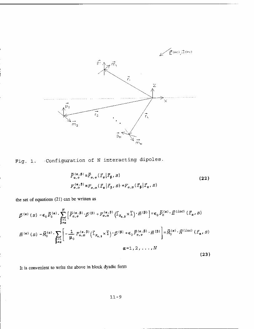
Pi A
£ (inc) |_| (inc)
Fig. 1. Configuration of N interacting dipoles
Kct.ß) = ̂Fe_e{fa\f.,S) e,e e, e v a
F^J^Feim(fa\f^s)=Feim(fp\la,s) (22)
the set of equations (21) can be written as
p<«><S)-e0iVtt)-EPereß)^^ =1
1*0
rn(a) (s) -M0(a) m
-±F^(iR^iypW+eQF^-ffiW
a=l,2,...,N
= M<a)-HUnc) (za,s)
(23)
It is convenient to write the above in block dyadic form
11-9
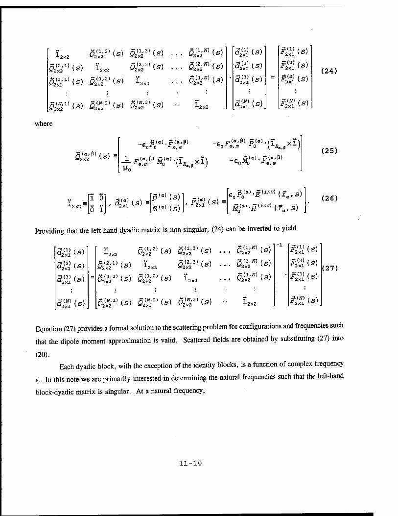
-"-2x2 S&a)<s> Sä'3)<*> ^2x2
1 2x2
2x2
Öä'1}<s> Q&2)(s) 1 2x2
a<V(s) Q£2)(S) Q£P(B)
$&*> (s)
Q&N) is)
L2x2
3£L <*>
3H is)
4ffi <*>
r2xl
F(2)
(S)
2X1 (S)
2x1 (S) F(3)
*V2<*>
(24)
where
&i'|,,(s)-
-e 8(«).?<«'P) -e F(°'p) P(oW:U xl\
— -e.» ^0 (1i?(«,pX1) ro
-6 M(o)-F("'P) C0XJ0 re,e
(25)
-2x2
1 0
0 1 .3&>(a) "2x1
p<B) [s)
ffi(a) (s) ' ^2x1 (S^
£ H(a)^(inc)(f ) •0*0
/$<■> .£<*«> (fB,s) (26)
Providing that the left-hand dyadic matrix is non-singular, (24) can be inverted to yield
3^1 (s)
3SJ <*>
3Ä2 <*>
-■-2x2
fö1' (s)
fö2)(s) 5&3)(fl> '2x2
1 2x2 £*2X2 (S'
S&^s) 0^2)(s) 1 -2x2
D^is) Q^2)(s) 5£3){S)
-. OS,'"«*)
L2x2
-1 £!(1) 2x1 F,1"-.' (3)
£5(2) 2x1 F^' (s)
(27) ^ <*>
i*ä»
Equation (27) provides a formal solution to the scattering problem for configurations and frequencies such
that the dipole moment approximation is valid. Scattered fields are obtained by substituting (27) into
(20). Each dyadic block, with the exception of the identity blocks, is a function of complex frequency
s. In this note we are primarily interested in determining the natural frequencies such that the left-hand
block-dyadic matrix is singular. At a natural frequency,
11-10
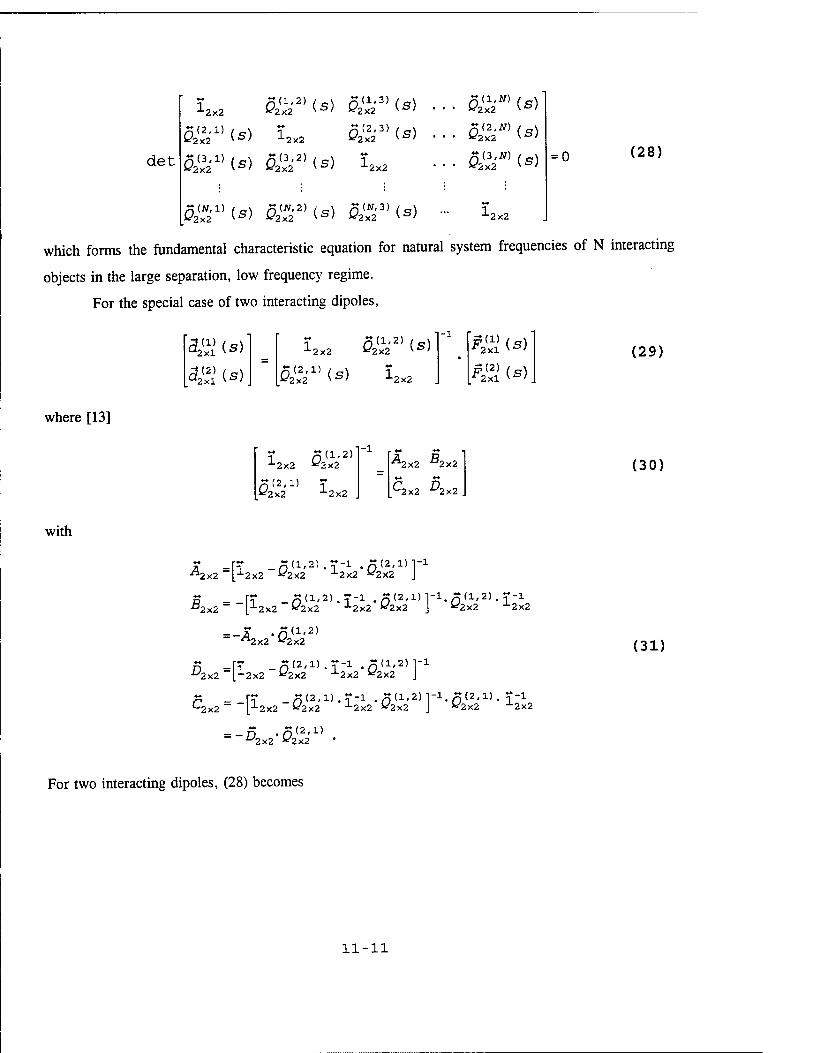
det
J-2x2
Q&1] is)
Q^Hs) Q, 2(^3)(s)
-2x2 Q&3)(s)
Q^fHs)
Q&1](s) fä'Us) i L2x2 «2x2 (S) = 0 (28)
OS^IB) %S2)(s) Q<»i3)(s) - l2x2
which forms the fundamental characteristic equation for natural system frequencies of N interacting
objects in the large separation, low frequency regime.
For the special case of two interacting dipoles,
3^1 (s) 3S I*)
-■-2x2
0^1](s) Q&2) is)
L2x2
-1 p(l) r2xl (s)
nil Is) (29)
where [13]
-■-2x2
g (2.1) «2x2
g(l,2) «2x2
1-1
-2x2
"^2x2 °2x2
^-2x2 ^2x2
(30)
with
A = Pf -n'1-2'.?-1 .5(2,i)]-i -™2x2 |X2x2 «2x2 x2x2 «2x2 J
s - _r? -n'1-2'.?-1 •O(2'1)r1-O(1'2)-1"1-, ^2x2 " |±2x2 «2x2 x2x2 «2x2 J «2x2 x2x2
^2x2 «2x2
s =pr -o'2'1»-!"1 •n(1'2)r1 ■^2x2 [J-2x2 «2x2 "L2x2 «2x2 J
* - r? _n(2-D.T-i .«(1.2)1-1.g(2.1). J-l C2x2 _ ~|12x2 «2x2 X2x2 «2x2 J «2x2 X2x2
•^2x2 «2x2
For two interacting dipoles, (28) becomes
(31)
11-11
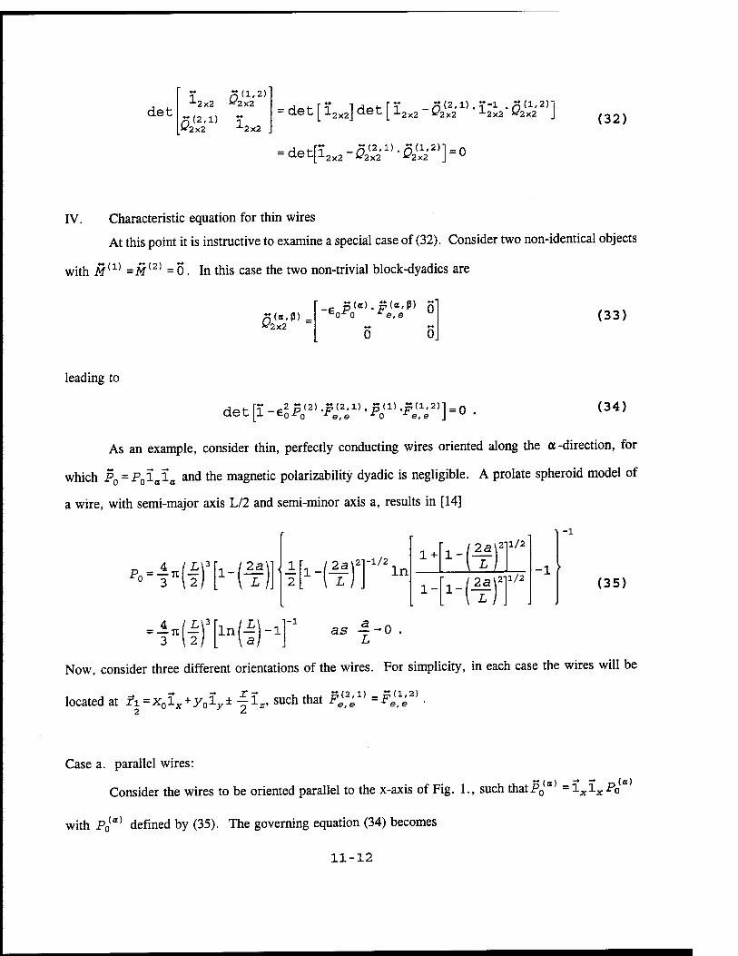
det J-2x2
X (2,1) ^2x2
*<1.2> ^2x2
L2x2
= det [ l2x2] det [ l2x2 -4x2X)' l2"x2- Ö2X22)]
= det[l2x2-52(x
22'1)-4x22)]=0
(32)
IV. Characteristic equation for thin wires
At this point it is instructive to examine a special case of (32). Consider two non-identical objects
with M[1) =M(2) = 0. In this case the two non-trivial block-dyadics are
^2x2
S(«>.S«*.ß> o (33)
leading to
detll-elP^-F^-P^-F^^O . (34)
As an example, consider thin, perfectly conducting wires oriented along the a -direction, for
which P0=P0lala and the magnetic polarizability dyadic is negligible. A prolate spheroid model of
a wire, with semi-major axis L/2 and semi-minor axis a, results in [14]
*.-Mi\'h- ffi _1 2
1- m ■1/2 In
1 +
1-
2a 2U/2
\HW -l
(35)
as -S-0 .
Now, consider three different orientations of the wires. For simplicity, in each case the wires will be
located at fi =x0lx+y0ly± -f lz, such that F^;x) = *(1,2)
2 ^ , e x e,e
Case a. parallel wires:
Consider the wires to be oriented parallel to the x-axis of Fig. 1., such thatP0 = lxlx P0
with P0(a) defined by (35). The governing equation (34) becomes
11-12
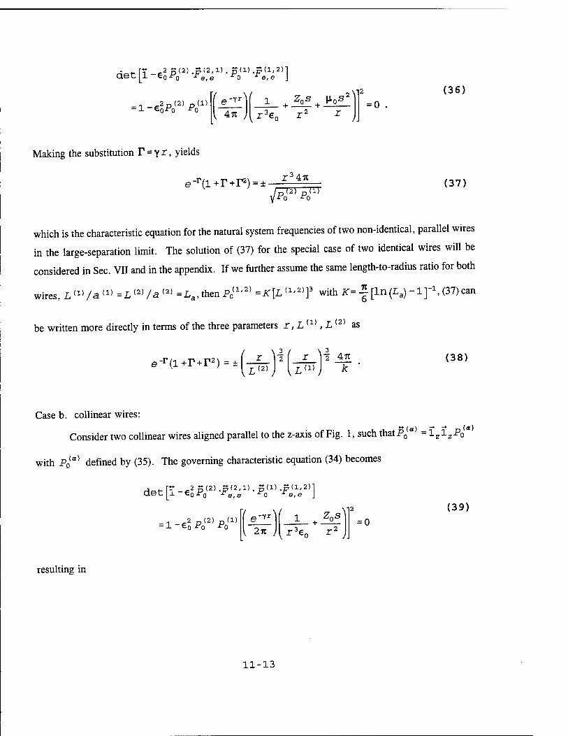
det[l-elP^'F^-Pr-?^2)]
-1 .Jp«) p(1) ,-Y-r
4TC
_1_ + JZQ£ + JVi M2
rJer
0 . (36)
Making the substitution T = yr, yields
e-r(i+r+r2) = ± r347t
(2) n(l) {W^O (37)
which is the characteristic equation for the natural system frequencies of two non-identical, parallel wires
in the large-separation limit. The solution of (37) for the special case of two identical wires will be
considered in Sec. VII and in the appendix. If we further assume the same length-to-radius ratio for both
)jL(i)/a(i)=L(2)/a(2)=La)thenP0(1'2)=iC[L(1'2)]3 withi<r=![ln(La)-:L]-\(37)can wires,
be written more directly in terms of the three parameters r,L{1), L (2) as
e-r(i+r+r2) = ±
\ 3 / \ 3 A
(2) (i)
(38)
Case b. collinear wires:
Consider two collinear wires aligned parallel to the z-axis of Fig. 1, such thatP0 ° =1Z1ZP0
with P0<a) defined by (35). The governing characteristic equation (34) becomes
det[l-elP^-F^-P^-F^}
= l-e2P0
<2)P0(1) e yT
v 271
1 ^ Zos
r3e r = 0
(39)
resulting in
11-13
-r,- . Tiv _ . r327t e-r(l+r) = ±-£-^— (40)
which is the characteristic equation for the natural system frequencies of two non-identical, collinear wires
in the large-separation limit. The solution of (40) for the special case of two identical wires will be
considered in the appendix. For L(1)/a(1) = L(2)/a(2> = La, suchthat P0(1'2) =K[Lll>2)]3 withic
as defined previously, (40) can be written as
e"r(l+r) = ± 2 / \ 3 2 z_ "2 _27C (4i)
(2) r (1)
Case c. perpendicularly-oriented wires:
To analyze two wires oriented perpendicularly to each other, one may take, for instance,
P(1) =1 1 P0(1) and P0
(2) =lzlzPo2) . The characteristic equation (34) becomes
detll-elP^-F^'P^'F^^detll-O^l (42)
so that no frequency exists to yield a singular matrix.
Additional details can be found in [15], where a separate formulation is provided for two objects
configured in a mirror-symmetric fashion.
VII. Numerical results
In order to demonstrate the accuracy of the presented formulation, the example of two identical,
thin, perfectly conducting parallel wires separated by a distance r=d is considered, as depicted in the
insert of Fig. 2. The wires are in a mirror-symmetric configuration, which admits pure symmetric and
antisymmetric modes. In all results to follow, both wires have L/a=200, and the natural frequencies in
the upper-half s-plane will be considered. For one such wire when isolated, the dominant resonance is
at JfiiiZ =-0.0865+J0.9386, computed from a rigorous electric-field integral equation (IE) using a
pulse basis and point matching [16]. Other resonances are available in the literature, e.g. [1].
For the coupled wire configuration described above, the asymptotic formulation (37) becomes
for L/a=200. The migration of the lowest-order anti-symmetric and symmetric mode as a function of
11-14
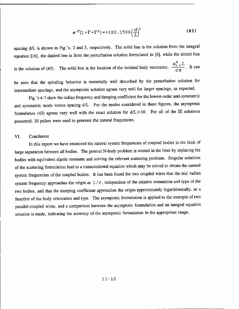
e-r(l+r + r2) = + 103.1596/-|)3 (43)
spacing d/L is shown in Fig.'s, 2 and 3, respectively. The solid line is the solution from the integral
equation [16], the dashed line is from the perturbation solution formulated in [6], while the dotted line
SlV is the solution of (43). The solid box is the location of the isolated body resonance, ' . It can
be seen that the spiraling behavior is essentially well described by the perturbation solution for
intermediate spacings, and the asymptotic solution agrees very well for larger spacings, as expected.
Fig.'s 4-7 show the radian frequency and damping coefficient for the lowest-order anti-symmetric
and symmetric mode versus spacing d/L. For the modes considered in these figures, the asymptotic
formulation (43) agrees very well with the exact solution for d/L> 10. For all of the IE solutions
presented, 20 pulses were used to generate the natural frequencies.
VI. Conclusion
In this report we have examined the natural system frequencies of coupled bodies in the limit of
large separation between all bodies. The general N-body problem is treated in the limit by replacing the
bodies with equivalent dipole moments and solving the relevant scattering problem. Singular solutions
of the scattering formulation lead to a transcendental equation which may be solved to obtain the natural
system frequencies of the coupled bodies. It has been found for two coupled wires that the real radian
system frequency approaches the origin as l/r, independent of the relative orientation and type of the
two bodies, and that the damping coefficient approaches the origin approximately logarithmically, as a
function of the body orientation and type. The asymptotic formulation is applied to the example of two
parallel-coupled wires, and a comparison between the asymptotic formulation and an integral equation
solution is made, indicating the accuracy of the asymptotic formulation in the appropriate range.
11-15
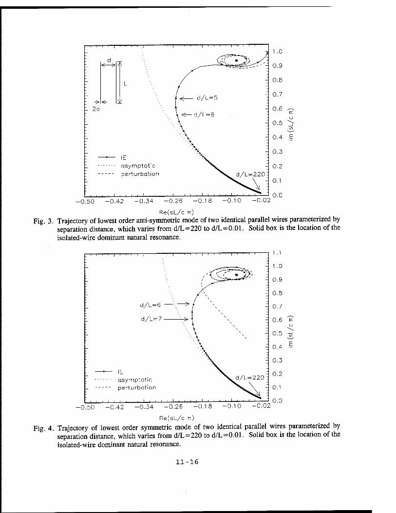
-l—i—i—[—r-
-, 1 .0
<—> A
\/ 2a
asymptotic perturbation
-0.50 -0.42 -0.34 -0.26 -0.18 -0.10 -0.02
Re(sL/c 7T)
Fig. 3. Trajectory of lowest order anti-symmetric mode of two identical parallel wires parameterized by separation distance, which varies from d/L=220 to d/L=0.01. Solid box is the location of the isolated-wire dominant natural resonance.
d/L=6
d/L=7
IE asymptotic perturbation
-0.50 -0.42 -0.34 -0.26 -0.18 -0.10 -0.02
Re(sL/c 7T)
Fig. 4. Trajectory of lowest order symmetric mode of two identical parallel wires parameterized by separation distance, which varies from d/L=220 to d/L=0.01. Solid box is the location of the isolated-wire dominant natural resonance.
11-16
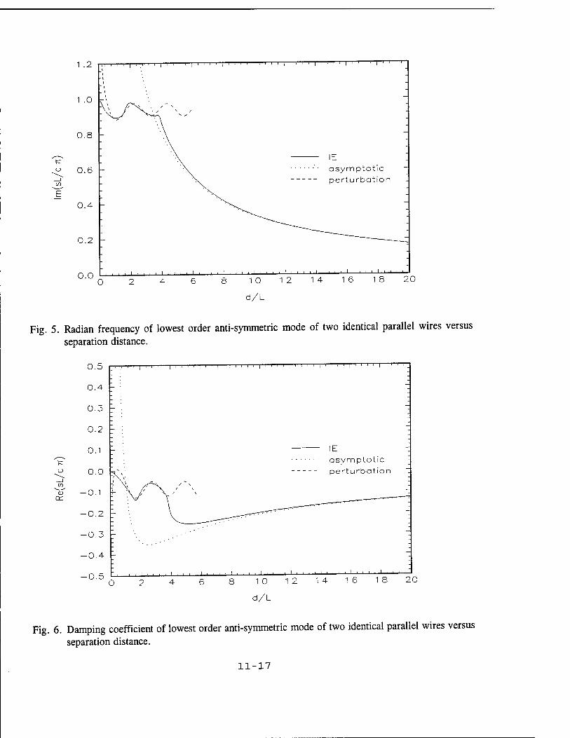
1 .2
1 .0
0.2
0.0
i i i i i , , , , i i ' ' ' ' I ' '
IE asymptotic perturbation
. i . , , , i
10 12 14 16 18 20
d/L
Fig. 5. Radian frequency of lowest order anti-symmetric mode of two identical parallel wires versus separation distance.
DC
0.5
0.4
0.3
0.2
0.1
0.0
-0.1
-0.2
-0.3
-0.4
-0.5 O
i i i i i i I ' ' ' ' I
asymptotic perturbation
8 10 12 14 16 18 20
d/L
Fig. 6. Damping coefficient of lowest order anti-symmetric mode of two identical parallel wires versus separation distance.
11-17
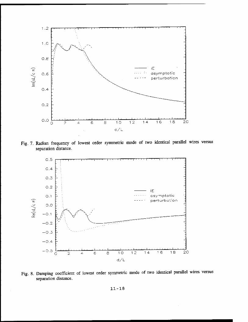
1 .2
1 .0
en
E
0.2
0.0
■,i i ' ' ' ' i ' ' ' ' i ' ■ ■ ■ i i i i | i i i i i i i i i i i ' '
IE asymptotic perturbation
. i .... i , . , , i , , i , i , i i
8 10 12 14 16 18 20
d/L
Fig. 7. Radian frequency of lowest order symmetric mode of two identical parallel wires versus separation distance.
0.5
0.4
0.3
0.2
0.1
0.0
-0.1
-0.2
-0.3
-0.4
-0.5
I I I'" I—I—I—I—| I I I '"'
IE asymptotic perturbation
i .... i
6 8 10 12 14
d/L
1 8 20
Fig. 8. Damping coefficient of lowest order symmetric mode of two identical parallel wires versus separation distance.
11-18
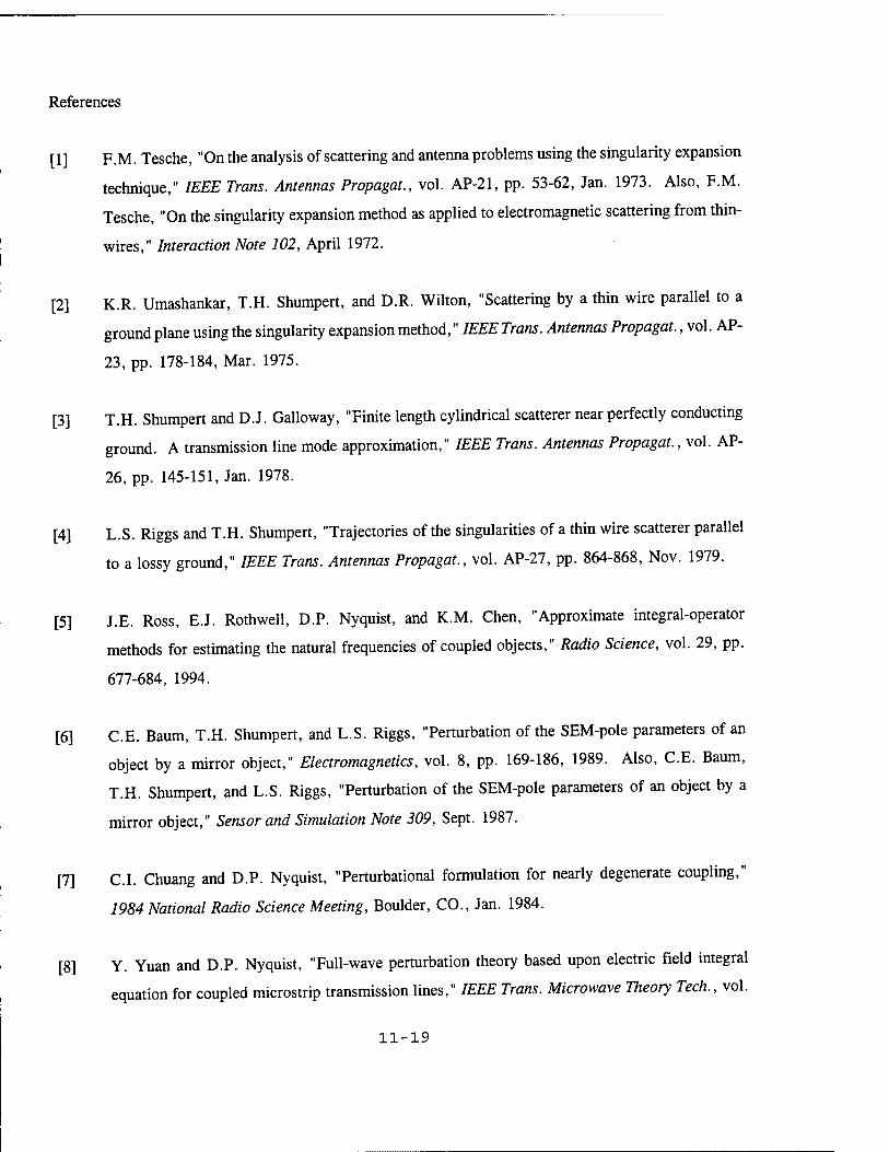
References
[1] F.M. Tesche, "On the analysis of scattering and antenna problems using the singularity expansion
technique," IEEE Trans. Antennas Propagat., vol. AP-21, pp. 53-62, Jan. 1973. Also, F.M.
Tesche, "On the singularity expansion method as applied to electromagnetic scattering from thin-
wires," Interaction Note 102, April 1972.
[2] K.R. Umashankar, T.H. Shumpert, and D.R. Wilton, "Scattering by a thin wire parallel to a
ground plane using the singularity expansion method," IEEE Trans. Antennas Propagat., vol. AP-
23, pp. 178-184, Mar. 1975.
[3] T.H. Shumpert and D.J. Galloway, "Finite length cylindrical scatterer near perfectly conducting
ground. A transmission line mode approximation," IEEE Trans. Antennas Propagat., vol. AP-
26, pp. 145-151, Jan. 1978.
[4] L.S. Riggs and T.H. Shumpert, "Trajectories of the singularities of a thin wire scatterer parallel
to a lossy ground," IEEE Trans. Antennas Propagat., vol. AP-27, pp. 864-868, Nov. 1979.
[5] J.E. Ross, E.J. Rothwell, D.P. Nyquist, and K.M. Chen, "Approximate integral-operator
methods for estimating the natural frequencies of coupled objects," Radio Science, vol. 29, pp.
677-684, 1994.
[6] C.E. Baum, T.H. Shumpert, and L.S. Riggs, "Perturbation of the SEM-pole parameters of an
object by a mirror object," Electromagnetics, vol. 8, pp. 169-186, 1989. Also, C.E. Baum,
T.H. Shumpert, and L.S. Riggs, "Perturbation of the SEM-pole parameters of an object by a
mirror object," Sensor and Simulation Note 309, Sept. 1987.
[7] C.I. Chuang and D.P. Nyquist, "Perturbational formulation for nearly degenerate coupling,"
1984 National Radio Science Meeting, Boulder, CO., Jan. 1984.
[8] Y. Yuan and D.P. Nyquist, "Full-wave perturbation theory based upon electric field integral
equation for coupled microstrip transmission lines," IEEE Trans. Microwave Theory Tech., vol.
11-19
38, pp. 1576-1584, Nov. 1990.
[9] G.W. Hanson and D.P. Nyquist, "Full-wave perturbation theory for the analysis of coupled
microstrip resonant structures," IEEE Trans. Microwave Theory Tech., vol. 40, pp. 1774-1779,
Sept. 1992.
[10] J. Van Bladel, Singular Electromagnetic Fields and Sources, Oxford Univ. Press, New York,
1991.
[11] A.D. Yaghjian, "Electric dyadic Green's functions in the source region," Proc. IEEE, vol. 68,
pp. 248-263, Feb. 1980.
[12] C. E. Baum, " Some characteristics of electric and magnetic dipole antennas for radiating transient
pulses, " Sensor and Simulation Note 125, Jan., 1971.
[13] C.E. Baum, T.K. Liu, and F.M. Tesche, "On the analysis of general multiconductor
transmission-line networks, " Interaction Note 350, Nov, 1978.
[14] K.S.H. Lee, "Electrically-small ellipsoidal antennas, " Sensor and Simulation Note 193, Feb.,
1974.
[15] G.W. Hanson and C.E. Baum, "Asymptotic Analysis of the Natural System Modes of Coupled
Bodies in the Large Separation, Low-Frequency Regime, " Interaction Note 528, July, 1997.
[16] J.E. Ross, private communication.
11-20
BLIND BAYESIAN RESTORATION OF ADAPTIVE OPTICS IMAGES USING GENERALIZED GAUSSIAN MARKOV RANDOM FIELD
MODELS
Brian D. Jeffs Associate Professor
Department of Electrical and Computer Engineering
Brigham Young University 459 CB
Provo, UT 84602
Final Report for: Summer Faculty Research Program
Phillips Laboratory
Sponsored by: Air Force Office of Scientific Research
Boiling Air Force Base, DC
And
Phillips Laboratory
September, 1998
12-1
BLIND BAYESIAN RESTORATION OF ADAPTIVE OPTICS IMAGES USING GENERALIZED GAUSSIAN MARKOV
RANDOM FIELD MODELS
Brian D. Jeffs Associate Professor
Department of Electrical and Computer Engineering Brigham Young University
Abstract
This report introduces a blind method based on Bayesian maximum a posteriori (MAP) estimation theory for restoring images corrupted by noise and blurred by one or more unknown point-spread-functions (psf). The paper addresses post processing for resolution enhancement of sequences of short exposure (2-10 ms) adaptive optics (AO) images of space objects. In the problem formulation, both the true image and the unknown blur psf's are represented by the flexible generalized Gaussian Markov random field (GGMRF) model. The GGMRF probability density function provides a natural mechanism for expressing available prior information about the image and blur. Incorporating such prior knowledge in the deconvolution optimization is crucial for the success of blind restoration algorithms. For example, space objects often contain sharp edge boundaries and geometric structures, while the residual blur psf in the corresponding partially corrected AO image is spectrally band limited, and exhibits smoothed, random, texture-like features on a peaked central core. By properly choosing parameters, GGMRF models can accurately represent both the blur psf and the object, and serve to regularize the deconvolution problem. These two GGMRF models also serve as discriminator functions to separate blur and object in the solution. Algorithm performance is demonstrated with examples from AO images collected at the Starfire Optical Range, USAF Phillips Laboratory. Results from both real and synthetic data indicate significant resolution enhancement when applied to partially corrected AO images. An efficient computational algorithm is described.
12-2
BLIND BAYESIAN RESTORATION OF ADAPTIVE OPTICS IMAGES USING GENERALIZED GAUSSIAN MARKOV
RANDOM FIELD MODELS1
Brian D. Jeffs
1 Introduction
This report introduces a blind method based on Bayesian maximum a posteriori (MAP) estimation theory for restoring images corrupted by noise and blurred by one or more unknown point-spread-functions (psf). A major advantage of this MAP approach is that it provides a natural (rather than ad-hoc) mechanism for incorporating prior information about the image and blur. Use of this prior knowledge is crucial for the success of blind algorithms. This information is expressed in the form of an image probability density function model, and serves as a regularizing term in the associated inverse problem.
The term "blind" as used in this paper refers to a wide variety of uncertainty levels regarding the blur psf's. For example, the available psf prior information may consist of high quality blur estimates or parametric analytical models. At the other extreme, blur knowledge may be limited to simply knowing the psf is non-negative and spectrally band limited. The proposed method permits a natural representation of any of these degrees of psf uncertainty in the blur model, and permits refining the blur estimate to be consistent with each frame observation.
Though the algorithm presented here may be used in a wide variety of blind deconvolution applications, we are particularly interested in high resolution restoration of multiframe adaptive optics (AO) telescopic images. AO systems can remove much of the atmospheric-turbulence-induced blur in astronomical and orbiting space objects imagery, but there is typically some adaptation error [1] [2] [3] [4]. Thus, a residual time-varying blur below the theoretical aperture cutoff resolution limit remains. Though the general structure of this residual blur is known [5] [6], the detail is not, and varies significantly over a period of milliseconds.
It is often impractical to acquire an accurate sample of the true residual psf by observing a nearby star. This residual blur is spatially varying, so a natural guide star may not be in the same isoplanatic patch as the object, and in the case of tracking space objects, no natural reference stars which follow the object are available. When observing bright objects, it is possible to acquire a sequence of high SNR, closely spaced (in time) frames with significant blur variation from frame to frame. This scenario is ideally suited to multi-frame blind deconvolution methods which exploit the blur diversity to solve the difficult blind problem.
As is usually the case, the blind restoration problem addressed here is complicated by the ill-posed nature of the associated inverse problem [7], and by the fact that blur psf, H, and the true object image, F can only be identified in combination (H * F) unless distinguishing prior information is available. This solution ambiguity is due to the commutative property of convolution which will yield the same observation regardless of whether a given image feature is contained in H or F. Therefore, the blind restoration problem is hopeless without a well formed method of expressing and imposing prior information on the solution. A number of authors have successfully applied various "hard" and "soft" constraints on the object and blur solutions as a means of incorporating prior information into the blind multiframe solution [2] [3] [1] [4] [8] [9] [10] [6].
The method presented here includes a new approach for incorporating image prior information in the blind problem. Probability density functions are used to statistically model available prior information about the structure of both the true image, F, and the blurring psf, H. We will show that adopting appropriate image and blur pdf models serves as a powerful discriminating constraint that leads to realistic estimates for both H and F. We will use the generalized Gaussian Markov random field model [11] because of its ability to represent a wide range of practical image types [12] [13]. It can accurately model both structured, hard edged fields typical of the true image, and smooth, "low pass" or "band limited" images typical of blurring psf's.
The availability of multiple observations with different but unknown blur psf's, Ht, can be a great aid in estimating F. The multiple frame observation reduces convolutional ambiguity because any image component that
'Sponsored by the Air Force Office of Scientific Research, Boiling Air Force Base, DC. The author acknowledges the contributions to this work from Dr. Julian C. Christou and Dr. Robert Fugate, Starfire Optical Range, USAF Phillips Laboratory.
12-3
is not common to all frames cannot be a component of the F. The method presented below will be developed to exploit this fact, and will be applicable for both single and multiple frame cases.
We adopt the following familiar linear image observation model
Gi = Hi*F + T)i, i=l---M (1)
where G, is the ith observed image frame, 77,- is additive noise, and '*' denotes 2-D convolution. G,-, Hi, F, and T)i are all assumed to be realizations of 2-D random fields, but F remains constant between observation frames. It will also be convenient to use the vector-matrix form of equation (1)
g, = H,f + Tji ■M (2)
where g,, f, and 77,- are now vectors formed by column scanning the corresponding 2-D images, and H, is the doubly block Toeplitz convolution matrix corresponding to h, [14].
The frame blur psf 's may be statistically correlated, so the optimal solution requires that the joint pdf across all frames be considered. For this case, when the H, are not independent, equation (2) must be augmented as
g
g
n
Hi + 77, where
[gl,g2,---.gM]T. fj= [77l,772,- ■■,T)M]T,
Hi
(3)
H M
2 Problem Formulation
Assuming f and % are statistically independent (a reasonable assumption in practice), the blind MAP restoration problem may be stated as
f,n = argmaxp/|A|g(f,^|g) I , rt
= argmaxpg|/,A(g|f,ft)p/(f)pA(70 (4)
In order to solve equation (4), we adopt the following density function models. Assuming the noise is zero mean, white Gaussian, the noise density is given by
1
Mv) 1
/-—MAT V27T a,
-e ^ 77*77
(5)
where ./V is the total number of pixels in the image field. The following development could also be easily adapted to a Poisson distribution noise model. This approach is favored by some authors in Adaptive Optics restoration because it more accurately characterizes photon noise in short exposure images [8]. Assuming that the noise is statistically independent from both the true image and the blur, the conditional probability of g given f and % can be trivially shown to be
Pg\fMs\f,fi) = Pvte-W)
f-—MN '27T a,
-JL(g-7tf)'(g-?tf) ■ e z<Ti (6)
The image is modeled as a generalized Gaussian Markov random field (GGMRF), with joint pdf given by the Gibbs distribution [11]
pf(f) = ^-exP< -ß J2 bs,t\f*-ft\p+J2a°tf°\p
<s,t>eCr s£Sf
(7)
12-4
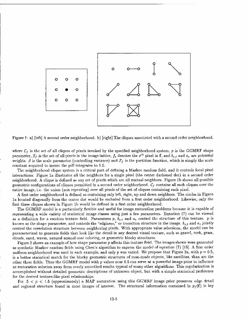
o o o
o • o
o o o
Figure 1: a) [left] A second order neighborhood, b) [right] The cliques associated with a second order neighborhood.
where C/ is the set of all cliques of pixels invoked by the specified neighborhood system, p is the GGMRF shape parameter, Sj is the set of all pixels in the image lattice, f, denotes the sth pixel in f, and bStt and as are potential weights, ß is the scale parameter (controlling variance) and Zj is the partition function, which is simply the scale constant required to insure the pdf integrates to 1.0.
The neighborhood clique system is a critical part of defining a Markov random field, and it controls local pixel interactions. Figure la illustrates all the neighbors for a single pixel (the center darkened dot) in a second order neighborhood. A clique is defined as any set of pixels which are all mutual neighbors. Figure lb shows all possible geometric configurations of cliques permitted in a second order neighborhood. Cj contains all such cliques over the entire image, i.e. the union (non repeating) over all pixels of the set of cliques containing each pixel.
A first order neighborhood is defined as containing only left, right, up and down neighbors. The circles in Figure la located diagonally from the center dot would be excluded from a first order neighborhood. Likewise, only the first three cliques shown in Figure lb would be defined in a first order neighborhood.
The GGMRF model is a particularly flexible and useful for image restoration problems because it is capable of representing a wide variety of statistical image classes using just a few parameters. Equation (7) can be viewed as a definition for a random texture field. Parameters p, 6,>t and as control the structure of this texture, p is known as the shape parameter, and controls the "edginess," or transition structure in the image. 6S]t and as jointly control the correlation structure between neighboring pixels. With appropriate value selections, the model can be parameterized to generate fields that look like the detail in any desired visual texture, such as gravel, cork, grass, clouds, sand, waves, natural animal coat coloring, or geometric blocky structures.
Figure 2 shows an example of how shape parameter p affects this texture field. The images shown were generated as synthetic Markov random fields using Chen's algorithm to express the model of equation (7) [15]. A first order uniform neighborhood was used in each example, and only p was varied. We propose that Figure 2a, with p = 0.5, is a better statistical match for the blocky geometric structures of man-made objects, like satellites, than are the other three fields. Thus the GGMRF model with p values near 0.5 can serve as a powerful image prior to influence as restoration solution away from overly smoothed results typical of many other algorithms. This regularization is accomplished without detailed geometric descriptions of unknown object, but with a simple statistical preference for the desired texture-like pixel relationships.
For .5 < p < 1.5 (approximately) a MAP restoration using this GGMRF image prior preserves edge detail and regional structure found in most images of interest. The structural information contained in p/(f) is key
12-5
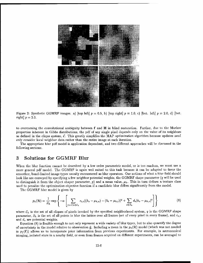
Figure 2: Synthetic GGMRF images, a) [top left] p right] p = 3.0.
0.5, b) [top right] p = 1.0, c) [bot. left] p - 2.0, d) [bot.
to overcoming the convolutional ambiguity between f and H in blind restoration. Further, due to the Markov properties inherent in Gibbs distributions, the pdf of any single pixel depends only on the value of its neighbors as defined in the clique system, C. This greatly simplifies the MAP optimization algorithm because updates need only consider local neighbor data rather than the entire image at each iteration.
The appropriate blur pdf model is application dependent, and two different approaches will be discussed in the following sections.
3 Solutions for GGMRF Blur
When the blur function cannot be described by a low order parametric model, or is too random, we must use a more general pdf model. The GGMRF is again well suited to this task because it can be adapted to favor the smoother, band-limited image types usually encountered as blur operators. Our notions of what a blur field should look like are conveyed by specifying a few neighbor potential weights, the GGMRF shape parameter (q will be used to distinguish it from the object shaper parameter, p) and a mean value, /*/,. This in turn defines a texture class used to penalize the optimization objective function if a candidate blur differs significantly from the model.
The GGMRF blur model is given by
ph(H) = — exp ^2 CMKA' <s.t>ech
■ ßh,>) - (ht - Vh,t)\q + ^2 ds\hs - fihy
sesh
(8)
where Ch is the set of all cliques of pixels invoked by the specified neighborhood system, q is the GGMRF shape parameter, Sh is the set of all points in blur the lattice over all frames (set of every pixel in every frame), and c,it
and ds are potential weights. Equation (8) is flexible enough to not only represent a wide variety of blur types, but to also quantify the degree
of uncertainty in the model relative to observation g. Including a mean in the PhCH) model (which was not needed in pj(f)) allows us to incorporate prior information from previous experiments. For example, in astronomical imaging, isolated stars in a nearby field, or even from frames acquired on different experiments, can be averaged to
12-6
serve as the reference mean. An analytic model can also be used as a mean. The Lorentzian function model may be used for residual AO blur [5] [6], or a simple Gaussian function for atmospheric turbulence. The GGMRF scale parameter, a, controls variance, and can be adjusted to match the degree of confidence in the GGMRF model as a whole. If the mean is a very good estimate of the actual blur, we set the scale parameter high (for low variance), and keep ds fairly large (positive) relative to cä](. If the mean estimate is very poor, ds is kept small, or zero, and all fih terms are dropped from equation (8). The model can then still impose the desired texture structure in %. If the blur is know to be spectrally band limited (e.g. bounded by the pupil cut off frequency), then the corresponding values of bs<t are large (relative to as), nearly uniform, and are all positive. It has been shown that for 1.75 < q < 3.0 and C/, corresponding to a first or second order uniformly weighted neighborhood, this model produces a random field with smoothed structures typical of many blur operators [13] [12].
Substituting equations (8),(7) and (6) into (4), and performing a little algebra yields
f,ft M
t=i
+A ^T, C>,t 1 (h> - Vh,,) ~ <s,t>ech
£ bs,t\f,-ft\p +
<s,t>€Ct
E' sesf
,\f.
{ht - ßh,t)\9 + Y^ ds\hs-ßh,Ag
s£Sh
(9)
where we have taken the logarithm of the r.h.s. (which does not change the maximization due to monotonicity) and have dropped additive constants. 7 and A control the relative influence, as regularizing terms, that the image and blur pdf's have respectively on the solution. If the neighborhood clique system, Ch does not include cliques that cross frame boundaries, then the H, are mutually independent, and equation (9) simplifies slightly to
f,n arg mm f,«
M
E t=i
|g,-H,-f||2 + A E cSit\{h, - fih.s) - {ht - fih,t)\q + Yl ds\hs Ph,. <s,t>£Ch, '€Shi
+7 <>,t>€C/
\f,-ft\p+Y,a<\f° (10)
where now Chi and 5A,- contain only cliques and pixels in the single frame, H,. The theoretical values 7 and A are functions of p, q, and the SNR, though exact expressions for are difficult
to derive. Therefor, these parameters are usually manually adjusted for most desirable results. The following proportionality relationships give some guidance on how to set 7 and A.
7 oc 2ßcr^, A oc 2aa^
Examples of restorations using the above formulation are presented in Section 6.
(11)
4 Solutions for Parametric Blur Models
In this section we develop a restoration solution for cases where significant detailed prior information regarding blur structure is available. This problem may be referred to as "semi-blind" or "myopic" restoration. Many common blurring functions, such out-of-focus and motion blurs, are well understood and can be accurately described using analytical psf models with one or two parameters [16] [17]. For example, if it is known a priori that blur is due to linear motion, the estimation problem can be reduced to simply finding the direction and extent of the motion. Rather than independently estimating every pixel in the psf, this two parameter estimation dramatically reduces the difficulty of blind restoration. Drummond has proposed a low order analytical model for AO residual blur based on a 2-D elliptic rotation of a Lorentzian function [5] [6]. This model requires only six parameters to fully describe the AO blur remaining in a partially corrected observation frame, and is a promising model for the AO space object restoration problem of interest.
For MAP restoration with parametric blur models we treat the parameters as random variables with an associated pdf, pe{0j), where 9, is the vector of blur model parameters for the ith frame. Applying this expression to equation
12-7
(4) and assuming f is independent of 0, yields
f,§ = argma_xp/%(f,0|g) f,e
= argm¥cpl,|/,«(g|f,'W(ö))p/(f)p,(Ä) (12) f ,8
where 0 = [6\, 02, ■ ■ ■, 0M]T and %{6) is a known deterministic matrix function of blur parameters, 0.
For polar parameters (e.g. orientation angle) we have used a uniform pdf model, pe(0i) = U(0,2ir). For most other parameters a Gaussian pdf model with a suitable mean value has proven adequate, though this choice is clearly arbitrary in many cases. Adopting a Gaussian blur parameter model and the GGMRF image prior distribution leads to the solution
M
fj = arg min V ||g; - H,-(0,-)f ||2 + 7 <s,t>£C, $esf
+ X(0 - ße)TR-\0 - ß9) (13)
where Rg = E{(0 — [iß)T(0 — ße)*T) and fi$ is the multiframe vector of parameter means specified by the operator. Examples of restoration using this formulation are presented in Section 6.
5 Optimization Algorithms
5.1 Metropolis Algorithm Implementation
Equation (4) is in general very difficult to solve since for most realistic pdf 's it is highly non-linear and has many local minima. This suggests that a stochastic optimization approach with randomized search strategy, such as the Metropolis algorithm for simulated annealing, is called for. The following procedural description adapts the Metropolis algorithm for use in blind, multiframe, GGMRF image restoration. The particular form shown has assumed both f and % are distributed GGMRF, but the algorithm is trivially modified to handle the parametric blur model of Section 4.
1. Choose an initial image, f° and initial blur frames, h? (e.g. f° = gi and h° = \ih)-
2. Set initial temperature, To.
3. Repeat for k = 1 to TV, the total number of iterations.
(a) Repeat for the total number of pixels in f.
i. Randomly choose a pixel site, s, without repeating.
ii. Generate a random variate, zs uniformly on A/, the set of allowed gray levels for f. iii. Assign ys = zs and yt = f£ \/t ^ s.
iv. Assign w = minjl, P^-fkC\Pfut'^t\\-
v. Replace fk with y with probability w, otherwise set fk+1 = fk.
(b) Repeat for i = 1 to M.
i. Repeat for the total number of pixels in h,-. A. Randomly choose a pixel site, s, without repeating. B. Generate a random variate, zs uniformly on A/,, the set of allowed gray levels for %.
C. Let V = [vi, • • -, Vjtf]T, where v,- = [wi,i, • •-,fi,iv]T- Assign w1|S = zs and w,|t = hkt V t ^ s.
Assign \j = hj V j ^ i.
U. Assign w - min^i, p^ifc(g|f*+iiW*)Pfc(fcjj^t Vi,t^) /•
E. Let Uk+l = V with probability w, otherwise set 7ik+1 = Uk-
12-8
loK(l+fc)' (c) Reduce temperature, Tk+\ = i0|(2+fcj^
Due to the Markov property of Gibbs distributions, the conditional probability densities in the above algorithm have a particularly simple form which depends only on the neighbors of pixel s. Additionally, since only ratios of density functions are considered, we may neglect all leading scale (partition function) terms.
M/,l/*v*#«) = M/TI/Metf.)
oc e £<e,/-«i'.*-rti,'+«.i/.*i'
Ph{hl.\hkjitVj,tj:s) = PH(hl,\htt€6.)
oc e A[£te4iC.,,|(/.,-^,.)-(Ai-/«k,«)|'+d.|A.-Mh,.|*]
(14)
(15)
where Ss is the small set of pixels neighboring pixel s as defined by the clique system C. Examples of restorations using this algorithm are presented in Section 6.
5.2 Steepest Descent Algorithm
For certain choices of the GGMRF parameters, equations (9) and (10) represent optimizations of convex functionals, and can therefore be solved using the much more efficient gradient descent techniques. Sufficient conditions for the model parameters to insure convex optimization are: q,p > 1, as,ds > 0 Vs, and 6s?t,cS)t > 0 Vs,i. If p = 2, then a necessary and sufficient condition for the image prior term to be convex is that B be a non-negative definite matrix with elements B,t related to equation (7) by Bst = -65|t, as = J2tes &>t, and Bst — 0 for s £ Ss. Ss is the set of neighboring pixels in all cliques containing fs. Similar constraints hold for c,it and ds if q — 2. These conditions are not overly restrictive. We have found that with p = 1.1 and q > 2 the image model preserves edge features, and the blur model imposes sufficient smoothness to separate f from %.
In order to simplify gradient computation, the objective function of equation (10) can be expressed as
J(f,H) = (g-W)T(g-7/f)+7Trace{Diag{^6t|f-Ptfn} tes.
+A Trace{Diag{d|h - ßh\q + £ c*l(h " Hh) ~ p'(h ~ /**)!*}} tesh
(16)
where | ■ \p indicates element-wise exponentiation of the magnitude and Diag{-} forms a diagonal matrix from a vector. We have assumed as — 0 ( a common choice [11]), and that b,it, cSit, and ds are constant with respect to s. This assumption restricts the model to homogeneous (spatially stationary) random fields. Pt is a permutation matrix which shifts f to align ft with /,. Sj and Sh are sets of indices used to select shifts consistent with the neighborhood structure of C. Since the field is stationary, these sets are independent of s. For example, in the case of a first order neighborhood, Sj would contain four indices to select up, down, left, and right neighbors. Neglecting edge effects, an example of Ps where t = "nearest neighbor down" would be as follows:
Pt
0 1 0 0
0 •• ■ 0 1 0 0 •• 0 1 0 •• 0
when t is the index for 1 row down. (17)
The derivative of equation (16) with respect to f is readily computed. However, to compute the derivative with respect to the i'/i frame blur, h,-, the first term of (16) is replaced with the equivalent expression £,=1 M(g - Fh,)T(g - Fhj), where F is the block Toeplitz convolution matrix formed from f.
M
^J(f,-H) = -2X)H?'(g.--H,-f) + ap5]6tQ?'|Qtfr1©sign{Qtf} at ;=i tea/
(18)
12-9
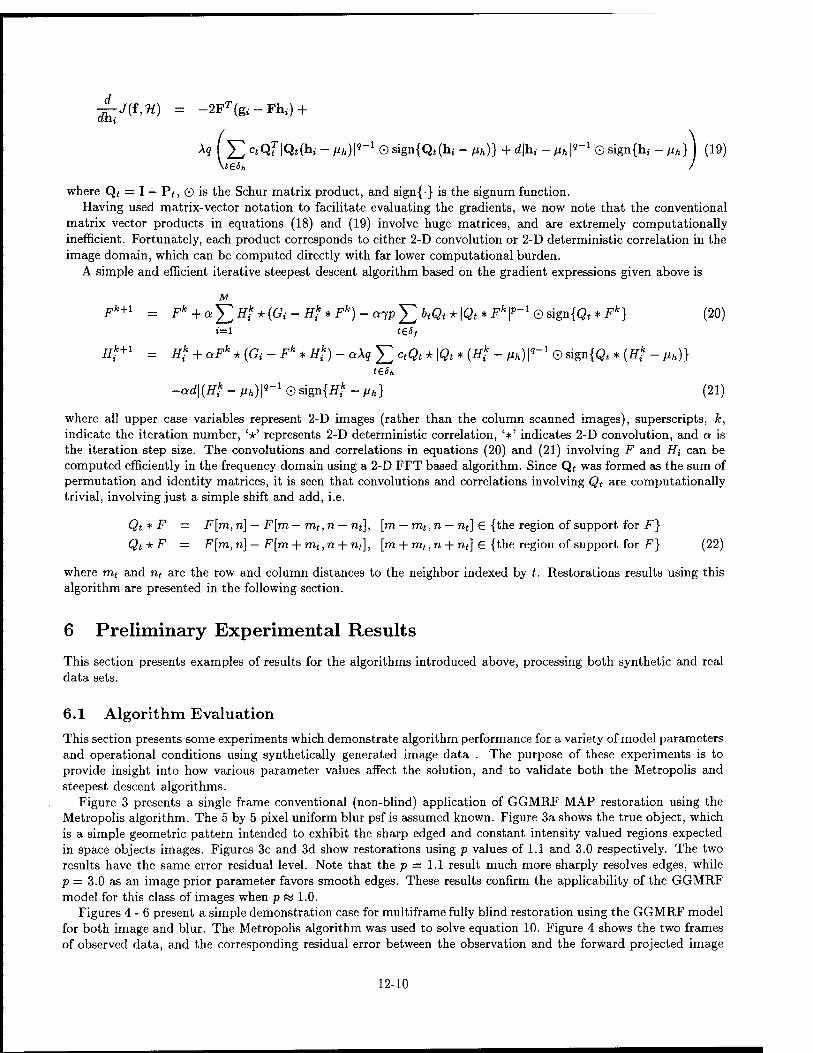
^J(f^) = -2FT(gi - Phi) +
Xq I J2 ctQf\Qt(hi - /M)!«-1 © sign{Qt(h,- - fih)} + d|h,- - ßh\q~l © sign{hi - p.h} ) (19)
where Qt = I — P^, © is the Schur matrix product, and sign{} is the signum function. Having used matrix-vector notation to facilitate evaluating the gradients, we now note that the conventional
matrix vector products in equations (18) and (19) involve huge matrices, and are extremely computationally inefficient. Fortunately, each product corresponds to either 2-D convolution or 2-D deterministic correlation in the image domain, which can be computed directly with far lower computational burden.
A simple and efficient iterative steepest descent algorithm based on the gradient expressions given above is
M
Fh+i = F* + aY/H?*{Gi-H?*Fk)-aypy}2btQt*\Qt*Fk\P-1QSign{Qt*Fk} (20) J=I test
Hk+i = Rk + aFk ^ (G. _ Fk t H^ _ aXq ^2 ctQt * \Qt * (iff - /ift)!'-1 © sign{Q( * (jtf - fih)} tesh
-ad\(Hk - ßh)?-1 © sign{#f - nh} (21)
where all upper case variables represent 2-D images (rather than the column scanned images), superscripts, k, indicate the iteration number, '*' represents 2-D deterministic correlation, '*' indicates 2-D convolution, and a is the iteration step size. The convolutions and correlations in equations (20) and (21) involving F and Hi can be computed efficiently in the frequency domain using a 2-D FFT based algorithm. Since Qt was formed as the sum of permutation and identity matrices, it is seen that convolutions and correlations involving Qt are computationally trivial, involving just a simple shift and add, i.e.
Qt * F = F[m, n] — F[m — mt,n — nt], [m — mt,n — nt] € {the region of support for F}
Qt* F = F[m, n] — F[m + nit, n + nt], [m + mt,n + nt] G {the region of support for F} (22)
where mt and nt are the row and column distances to the neighbor indexed by t. Restorations results using this algorithm are presented in the following section.
6 Preliminary Experimental Results
This section presents examples of results for the algorithms introduced above, processing both synthetic and real data sets.
6.1 Algorithm Evaluation
This section presents some experiments which demonstrate algorithm performance for a variety of model parameters and operational conditions using synthetically generated image data . The purpose of these experiments is to provide insight into how various parameter values affect the solution, and to validate both the Metropolis and steepest descent algorithms.
Figure 3 presents a single frame conventional (non-blind) application of GGMRF MAP restoration using the Metropolis algorithm. The 5 by 5 pixel uniform blur psf is assumed known. Figure 3a shows the true object, which is a simple geometric pattern intended to exhibit the sharp edged and constant intensity valued regions expected in space objects images. Figures 3c and 3d show restorations using p values of 1.1 and 3.0 respectively. The two results have the same error residual level. Note that the p = 1.1 result much more sharply resolves edges, while p — 3.0 as an image prior parameter favors smooth edges. These results confirm the applicability of the GGMRF model for this class of images when p & 1.0.
Figures 4-6 present a simple demonstration case for multiframe fully blind restoration using the GGMRF model for both image and blur. The Metropolis algorithm was used to solve equation 10. Figure 4 shows the two frames of observed data, and the corresponding residual error between the observation and the forward projected image
12-10
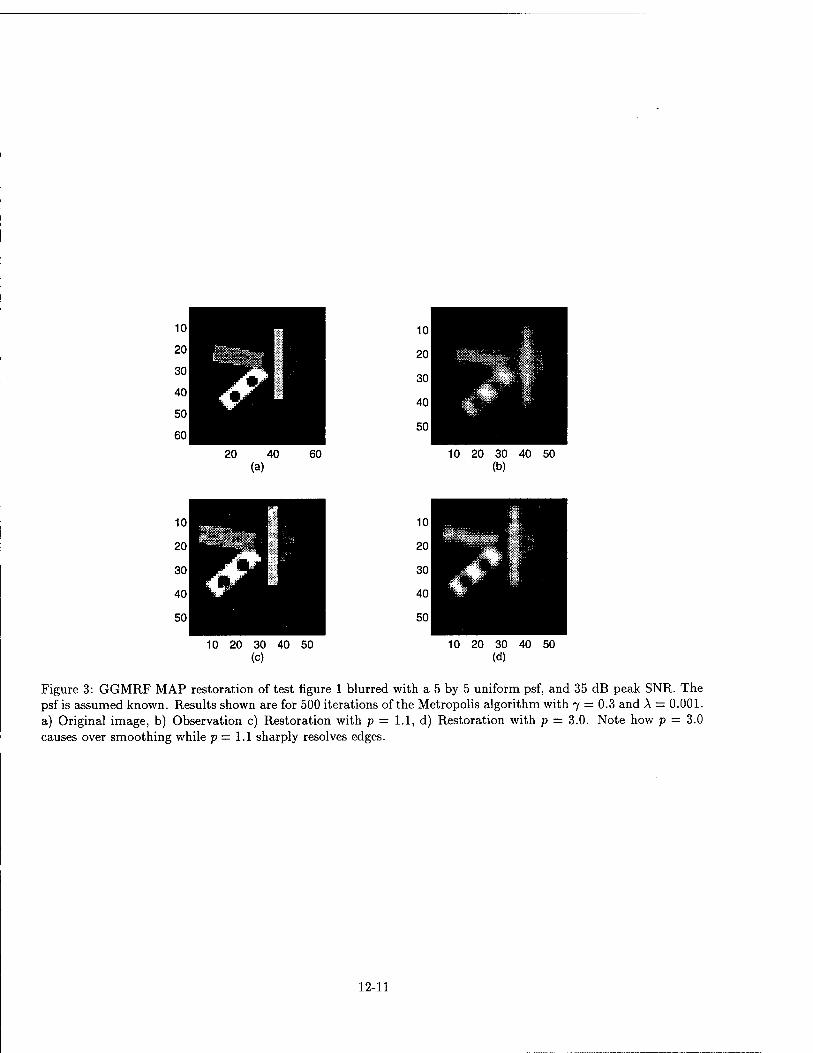
10 20 30 40 50 (b)
10 20 30 40 50 (c)
10 20 30 40 50 (d)
Figure 3: GGMRF MAP restoration of test figure 1 blurred with a 5 by 5 uniform psf, and 35 dB peak SNR. The psf is assumed known. Results shown are for 500 iterations of the Metropolis algorithm with 7 = 0.3 and A = 0.001. a) Original image, b) Observation c) Restoration with p = 1.1, d) Restoration with p = 3.0. Note how p = 3.0 causes over smoothing while p = 1.1 sharply resolves edges.
12-11
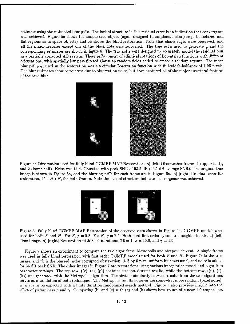
estimate using the estimated blur psf s. The lack of structure in this residual error is an indication that convergence was achieved. Figure 5a shows the simple true object (again designed to emphasize sharp edge boundaries and flat regions as in space objects) and 5b shows the blind restoration. Note that sharp edges were preserved, and all the major features except one of the black dots were recovered. The true psf's used to generate g and the corresponding estimates are shown in figure 6. The true psf's were designed to accurately model the residual blur in a partially corrected AO system. These psf's consist of elliptical rotations of Lorentzian functions with different orientations, with spatially low pass filtered Gaussian random fields added to create a random texture. The mean blur psf, fijj, used in the restoration was a a circular Lorentzian function with full-width-half-max of 1.25 pixels. The blur estimates show some error due to observation noise, but have captured all of the major structural features of the true blur.
SR^SSEöTO
Figure 4: Observation used for fully blind GGMRF MAP Restoration, a) [left] Observation frames 1 (upper half), and 2 (lower half). Noise was i.i.d. Gaussian with peak SNR of 53.5 dB (46.1 dB average SNR). The original true image is shown in Figure 5a, and the blurring psf's for each frame are in Figure 6a. b) [right] Residual error for restoration, G — H * F, for both frames. Note the lack of structure indicates convergence was achieved.
Figure 5: Fully blind GGMRF MAP Restoration of the observed data shown in Figure 4a. GGMRF models were used for both F and H. For F, p = 0.8. For H, q = 2.5. Both used first order symmetric neighborhoods, a) [left] True image, b) [right] Restoration with 3000 iterations, TO = 1, A = 10.0, and 7 = 1.0.
Figure 7 shows an experiment to compare the two algorithms, Metropolis and steepest descent. A single frame was used in fully blind restoration with first order GGMRF models used for both F and H. Figure 7a is the true image, and 7b is the blurred, noise corrupted observation. A 5 by 5 pixel uniform blur was used, and noise is added for 35 dB peak SNR. The other images in Figure 7 are restorations using various image prior model and algorithm parameter settings. The top row, ((c), (e), (g)) contains steepest descent results, while the bottom row, ((d), (f), (h)) was generated with the Metropolis algorithm. The obvious similarity between results from the two algorithms serves as a validation of both techniques. The Metropolis results however are somewhat more random (pixel noise), which is to be expected with a finite duration randomized search method. Figure 7 also provides insight into the effect of parameters p and 7. Comparing (b) and (c) with (g) and (h) shows how values of p near 1.0 emphasizes
12-12
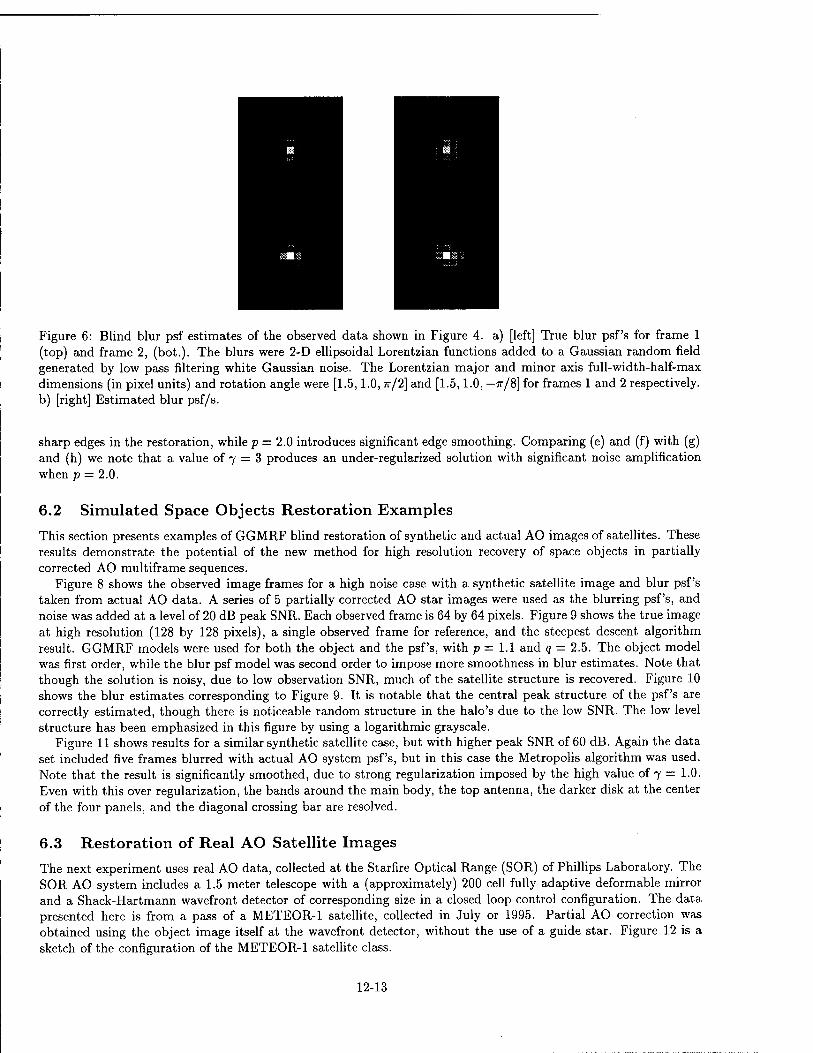
Figure 6: Blind blur psf estimates of the observed data shown in Figure 4. a) [left] True blur psf's for frame 1 (top) and frame 2, (bot.). The blurs were 2-D ellipsoidal Lorentzian functions added to a Gaussian random field generated by low pass filtering white Gaussian noise. The Lorentzian major and minor axis full-width-half-max dimensions (in pixel units) and rotation angle were [1.5,1.0,7r/2] and [1.5,1.0, — 7r/8] for frames 1 and 2 respectively, b) [right] Estimated blur psf/s.
sharp edges in the restoration, while p = 2.0 introduces significant edge smoothing. Comparing (e) and (f) with (g) and (h) we note that a value of 7 = 3 produces an under-regularized solution with significant noise amplification when p = 2.0.
6.2 Simulated Space Objects Restoration Examples
This section presents examples of GGMRF blind restoration of synthetic and actual AO images of satellites. These results demonstrate the potential of the new method for high resolution recovery of space objects in partially corrected AO multiframe sequences.
Figure 8 shows the observed image frames for a high noise case with a synthetic satellite image and blur psf's taken from actual AO data. A series of 5 partially corrected AO star images were used as the blurring psf's, and noise was added at a level of 20 dB peak SNR. Each observed frame is 64 by 64 pixels. Figure 9 shows the true image at high resolution (128 by 128 pixels), a single observed frame for reference, and the steepest descent algorithm result. GGMRF models were used for both the object and the psf's, with p = 1.1 and q = 2.5. The object model was first order, while the blur psf model was second order to impose more smoothness in blur estimates. Note that though the solution is noisy, due to low observation SNR, much of the satellite structure is recovered. Figure 10 shows the blur estimates corresponding to Figure 9. It is notable that the central peak structure of the psf's are correctly estimated, though there is noticeable random structure in the halo's due to the low SNR. The low level structure has been emphasized in this figure by using a logarithmic grayscale.
Figure 11 shows results for a similar synthetic satellite case, but with higher peak SNR of 60 dB. Again the data set included five frames blurred with actual AO system psf's, but in this case the Metropolis algorithm was used. Note that the result is significantly smoothed, due to strong regularization imposed by the high value of 7 = 1.0. Even with this over regularization, the bands around the main body, the top antenna, the darker disk at the center of the four panels, and the diagonal crossing bar are resolved.
6.3 Restoration of Real AO Satellite Images The next experiment uses real AO data, collected at the Starfire Optical Range (SOR) of Phillips Laboratory. The SOR AO system includes a 1.5 meter telescope with a (approximately) 200 cell fully adaptive deformable mirror and a Shack-Hartmann wavefront detector of corresponding size in a closed loop control configuration. The data presented here is from a pass of a METEOR-1 satellite, collected in July or 1995. Partial AO correction was obtained using the object image itself at the wavefront detector, without the use of a guide star. Figure 12 is a sketch of the configuration of the METEOR-1 satellite class.
12-13
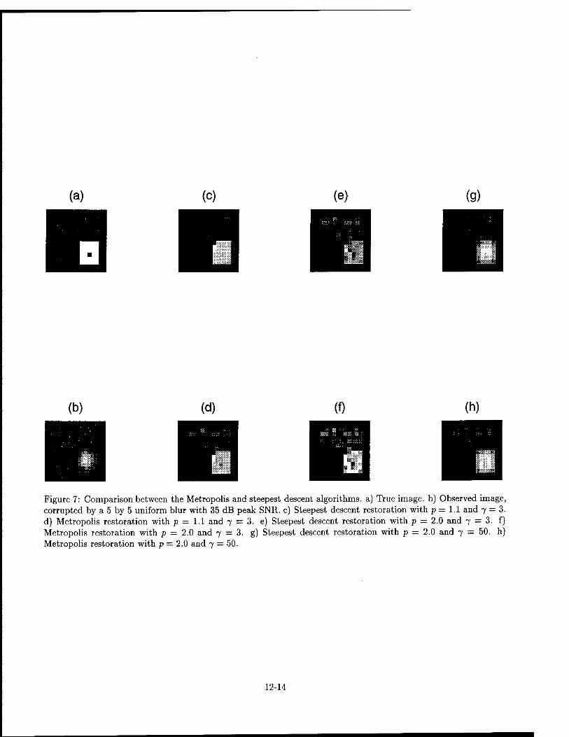
Figure 7: Comparison between the Metropolis and steepest descent algorithms, a) True image, b) Observed image, corrupted by a 5 by 5 uniform blur with 35 dB peak SNR. c) Steepest descent restoration with p = 1.1 and 7 = 3. d) Metropolis restoration with p = 1.1 and 7 = 3. e) Steepest descent restoration with p = 2.0 and 7 = 3. f) Metropolis restoration with p = 2.0 and 7 = 3. g) Steepest descent restoration with p = 2.0 and 7 = 50. h) Metropolis restoration with p = 2.0 and 7 = 50.
12-14
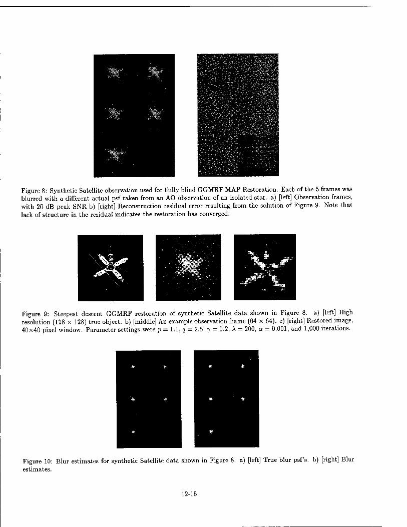
Figure 8: Synthetic Satellite observation used for Fully blind GGMRF MAP Restoration. Each of the 5 frames was blurred with a different actual psf taken from an AO observation of an isolated star, a) [left] Observation frames, with 20 dB peak SNR b) [right] Reconstruction residual error resulting from the solution of Figure 9. Note that lack of structure in the residual indicates the restoration has converged.
lÄä W* -ffim ■■■•■■ TL JKr
".jJ§§;JPä::>S l»ffi.
Figure 9: Steepest descent GGMRF restoration of synthetic Satellite data shown in Figure 8. a) [left] High resolution (128 x 128) true object, b) [middle] An example observation frame (64 x 64). c) [right] Restored image, 40x40 pixel window. Parameter settings were p = 1.1, q = 2.5, 7 = 0.2, A = 200, a = 0.001, and 1,000 iterations.
Figure 10: Blur estimates for synthetic Satellite data shown in Figure 8. a) [left] True blur psf's. b) [right] Blur estimates.
12-15
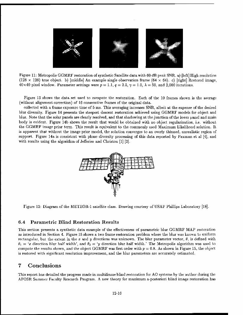
Figure 11: Metropolis GGMRF restoration of synthetic Satellite data with 60 dB peak SNR. a) [left] High resolution (128 x 128) true object, b) [middle] An example single observation frame (64 x 64). c) [right] Restored image, 40x40 pixel window. Parameter settings were p = 1.1, q = 2.5, 7 = 1.0, A = 50, and 2,000 iterations.
Figure 13 shows the data set used to compute the restoration. Each of the 10 frames shown is the average (without alignment correction) of 16 consecutive frames of the original data.
collected with a frame exposure time of 5 ms. This averaging increases SNR, albeit at the expense of the desired blur diversity. Figure 14 presents the steepest descent restoration achieved using GGMRF models for object and blur. Note that the solar panels are clearly resolved, and that shadowing at the junction of the lower panel and main body is evident. Figure 14b shows the result that would be obtained with no object regularization, i.e. without the GGMRF image prior term. This result is equivalent to the commonly used Maximum Likelihood solution. It is apparent that without the image prior model, the solution converges to an overly thinned, unrealistic region of support. Figure 14a is consistent with phase diversity processing of this data reported by Paxman et al [4], and with results using the algorithm of Jefferies and Christou [1] [2].
Figure 12: Diagram of the METEOR-1 satellite class. Drawing courtesy of USAF Phillips Laboratory [18].
6.4 Parametric Blind Restoration Results
This section presents a synthetic data example of the effectiveness of parametric blur GGMRF MAP restoration as introduced in Section 4. Figure 15 shows a two frame restoration problem where the blur was known to uniform rectangular, but the extent in the x and y directions was unknown. The blur parameter vector, 9, is defined with 61 = 'a; direction blur half width', and Ö2 = 'y direction blur half width.' The Metropolis algorithm was used to compute the results shown, and the object GGMRF was first order with p = 0.8. As shown in Figure 15, the object is restored with significant resolution improvement, and the blur parameters are accurately estimated.
7 Conclusions This report has detailed the progress made in multiframe blind restoration for AO systems by the author during the AFOSR Summer Faculty Research Program. A new theory for maximum a-posteriori blind image restoration has
12-16
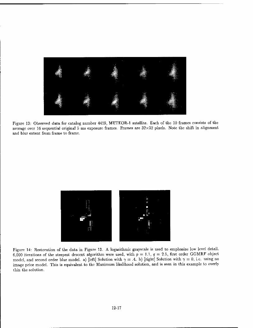
Figure 13: Observed data for catalog number 4419, METEOR-1 satellite. Each of the 10 frames consists of the average over 16 sequential original 5 ms exposure frames. Frames are 32x32 pixels. Note the shift in alignment and blur extent from frame to frame.
Figure 14: Restoration of the data in Figure 13. A logarithmic grayscale is used to emphasize low level detail. 6,000 iterations of the steepest descent algorithm were used, with p = 1.1, q = 2.5, first order GGMRF object model, and second order blur model, a) [left] Solution with 7 = .4. b) [right] Solution with 7 = 0, i.e. using no image prior model. This is equivalent to the Maximum likelihood solution, and is seen in this example to overly thin the solution.
12-17
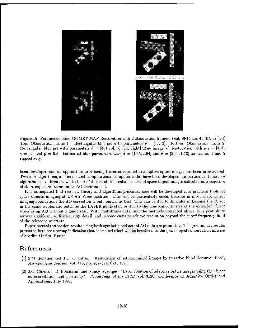
Figure 15: Parametric blind GGMRF MAP Restoration with 2 observation frames. Peak SNR was 40 dB. a) [left] Top: Observation frame 1 . Rectangular blur psf with parameters 6 = [1.5,3]. Bottom: Observation frame 2. Rectangular blur psf with parameters 6 — [4,1.75], b) [top right] True image, c) Restoration with fie = [3,3], 7 = .2, and p = 0.8. Estimated blur parameters were 6 = [1.45,2.94] and 0 = [3.96,1.73] for frames 1 and 2 respectively.
been developed and its application to reducing the error residual in adaptive optics images has been investigated. Two new algorithms, and associated computational computer codes have been developed. In particular, these new algorithms have been shown to be useful in resolution enhancement of space object images collected as a sequence of short exposure frames in an AO environment.
It is anticipated that the new theory and algorithms presented here will be developed into practical tools for space objects imaging at US Air Force facilities. This will be particularly useful because in most space object imaging applications the AO correction is only partial at best. This can be due to difficulty in keeping the object in the same isoplanatic patch as the LASER guide star, or due to the non-point-like size of the extended object when using AO without a guide star. With multiframe data, and the methods presented above, it is possible to recover significant additional edge detail, and in some cases to achieve resolution beyond the cutoff frequency limit of the telescope aperture.
Experimental restoration results using both synthetic and actual AO data are promising. The preliminary results presented here are a strong indication that continued effort will be beneficial to the space objects observation mission of Starfire Optical Range.
References
[1] S.M. Jefferies and J.C. Christou, "Restoration of astrononmical images by iterative blind deconvolution", Astrophysical Journal, vol. 415, pp. 862-874, Oct. 1993.
[2] J.C. Christou, D. Bonaccini, and Nancy Ageorges, "Deconvolution of adaptive optics images using the object autocorrelation and positivity", Proceedings of the SPIE, vol. 3126: Conference on Adaptive Optics and Applications, July 1997.
12-18

[3] JM. Conan, L. Laurent, T. Fusco, V. Michau, and G. Rousset, "Deconvolution of adaptive optics images using the object autocorrelation and positivity", Proceedings of the SPIE, vol. 3126: Conference on Adaptive Optics and Applications, July 1997.
[4] R.B. Paxman, J.H. Seldin, B.J. Thelen, M.F. Reiley, and D.A. Carrarra, "Focused-beam scoring techniques, volume i", Tech. Rep. 278140-9-F(V.I), SOR, Air Force Phillips Laboratory, Kirtland AFB, 1997.
[5] J.D. Drummond, "Sizes, shapes and rotational poles of ceres and vesta from adaptive optics images", Bulletin of the American Astronomical Society, vol. 27, pp. 16, 1996.
[6] J.D. Drummond, R.Q. Fugate, J.C. Christou, and E.K. Hege, "Full adaptive optics imgaes of asteroids ceres and vesta: Rotational poles and triaxial ellipsoid dimensions", to appear in ICARUS, 1998.
[7] R. L. Lagendijk and J. Biemond, Iterative Identification and Restoration of Images, Klewer, Boston, 1991.
[8] P.J. Sementilli, M.S. Nadar, and B.R. Hunt, "Poisson map super-resolution estimator with smooothness constraint", Proceedings of the SPIE, vol. 2032, July 1993.
[9] Y. Yang, N.P. Galatsanos, and H. Stark, "Projection-based blind deconvolution", Journal of the Optical Society of America A, vol. 11, no. 9, Sept. 1994.
[10] Z. Mou-yan and R. Unbehauen, "New algorithms of two-dimensioan blind deconvolution", Optical Engineering, vol. 34, no. 10, pp. 2945-2956, Oct. 1995.
[11] C. Bouman and K. Sauer, "A generalized Gaussian image model for edge-preserving MAP estimation", IEEE Transactions on Image Processing, vol. 2, no. 3, pp. 296-310, July 1993.
[12] Wai Ho Pun, Parametric Model-Adaptive Image Restoration, PhD thesis, Brigham Young University, 1995.
[13] W. H. Pun and B. D. Jeffs, "Shape parameter estimation for generalized gaussian markov random field models used in map image restoration", in Conference Record, 29th Asilomar Conf. Signals, Syst., Comp., Oct. 1995, pp. 1472-1476.
[14] A. K. Jain, Fundamentals of Digital Image Processing, Prentice Hall, Englewood Cliffs, 1989.
[15] C. C. Chen, Markov random field models in image analysis, PhD thesis, Michigan State University, East Lansing, 1988.
[16] R.C. Gonzalez and R.E. Woods, Digital Image Processing, Addison-Wesley, Reading, Massachusetts, 1992.
[17] J.W. Goodman, Fourier Optics, McGraw-Hill, New York, 1964.
[18] N.L. Johnson and D.M. Rodvold, "Europe and asia in space, 1993-1994", Tech. Rep., USAF Phillips Labora- tory/XPF, Kirtland AFB, NM, 1994.
12-19
MECHANICS OF SURFACE PRECISION FOR MEMBRANE REFLECTORS
Dr. Christopher H. M. Jenkins, P. E. Associate Professor
Department of Mechanical Engineering
South Dakota School of Mines and Technology 501 E. Saint Joseph Street
Rapid City, SD 57701
Final Report for: Summer Research Program
Phillips Laboratory
Sponsored by: Air Force Office of Scientific Research
Boiling Air Force Base, Washington, DC
And
Phillips Laboratory
September, 1997
10-1
MECHANICS OF SURFACE PRECISION FOR MEMBRANE REFLECTORS
Dr. Christopher H. M. Jenkins, P.E. Associate Professor
Director, Compliant Structures Laboratory Mechanical Engineering Department
South Dakota School of Mines and Technology
Abstract
The seminal application of membrane structures for space-based communications occurred
over four decades ago with the Echo series of satellites. Today, a resurgence of interest in
membrane structures for extraterrestrial use is developing, due to their potential for reduced launch
mass and stowed volume. Applications for such structures range from planar configurations in
solar sails, concentrators, and shields, to inflatable lenticulars for radar, radio, and optical uses.
The performance of this latter class of applications is studied, with particular emphasis on the
precision of the reflector surface.
13-2
MECHANICS OF SURFACE PRECISION FOR MEMBRANE REFLECTORS
Christopher H. M. Jenkins
INTRODUCTION
The seminal application of membrane structures for space-based communications occurred
over four decades ago with the Echo series of satellites [Shortal, 1978]. Today, a resurgence of
interest in membrane structures for extraterrestrial use is developing, due to their potential for
reduced launch mass and stowed volume. Applications for such structures range from planar
configurations in solar sails, concentrators, and shields, to inflatable lenticulars for radar, radio, and
optical uses.
Three key factors are paramount for the success and user acceptance of this technology:
manufacture, deployment, and performance. Performance hinges critically on the precision of the
membrane surface. The amount of precision is highly mission dependent, and may entail one or
more of the following issues: surface smoothness, deviation from desired surface profile, and slope
error.
A range of precision requirements exist. At one end are the solar sails and planar
concentrators which require maximum exposed surface area and/or flatness. At the other extreme,
membrane optical reflectors may require ratios of aperture diameter to figure error (rms) around 10
to 107 or more [Rapp, 1996].
For example, the AF Phillips Laboratory has recently undertaken the task of creating a large
optical quality membrane telescope. The membranes on these telescopes will range in thickness
from 10 - 150 micrometers. The maximum acceptable peak-to-peak figure error over the entire
surface will range from 10-20 micrometers. (This value assumes that a certain amount of
secondary adaptive optics will be used to correct image errors.)
THEORETICAL BASIS
Background
The problem of the inflation of an initially plane membrane with circular boundary begins
with Hencky [1915]. Earlier, Föppl [1907] had arrived at equilibrium equations for a membrane
plate. These equations were essentially modified von Kärmän plate equations [1910] with the
bending rigidity set to zero. Figure 1 represents a plane elastic sheet with circular boundary of
13-3
radius a. The geometry is rotationally symmetric (axisymmetric); we also assume the loading to be
a symmetric pressure p. The sheet has modulus E, thickness h, and Poisson's ratio v
The von Kärmän plate equations are based upon strains which have nonlinearity introduced
through rotations (squares of slope):
du 1 sr=— + -
dr 2
Uw^2
dr) (1)
£a=- (2)
where u and w are displacements in the r and z directions, respectively.
The von Kärmän plate equations in axisymmetric form can be written as:
D dr1
h d fdO dw^
r drydr dr ) = P (3)
1d2<S> 1#
dr dr' r dr
E + —
2
fdw^2
dr) (4)
where D = Eh3/12(l-v2) is the bending rigidity, and O is a stress function to which the stress
resultants in the radial and circumferential direction are related respectively by:
1JO Nr= ,Ng= ,
r dr dr
d2® d -£K) (5)
Linear elastic constitutive relations are assumed. It is important to note that the above equations are
not geometrically exact, in that several assumptions have been made.
Hencky provided a solution of the above for the case of zero boundary displacements (u = 0
= w at r = a) and D = 0 by assuming power series for stresses and transverse displacement. Little
interest in the Hencky problem seems to have taken place until the 1940's, when, in conjunction
with a study on air-supported roofs, Stevens [1944] performed an experimental investigation on a
10 inch radius by 0.014 inch thick cellulose acetate butyrate inflated circular membrane. Stevens
compared his results for the deflected membrane shape (which were apparently empirical in nature)
with Hencky's. Apparently Chien [1948] provided slight corrections to Hencky's solutions for
maximum values of stress and transverse deflection [see also Kao and Perrone, 1971].
13-4
Cambell [1956] allowed an arbitrary initial tension in the membrane. Dickey [1967] re-
examined the Hencky problem, this time using a nonlinear integral equation formulation. Dickey
provided a plot of u(r) for various values of the Poisson's ratio. Weil and Newmark [1955] provide
some experimental evidence that validate Dickey's predictions. We discuss later the important
relationship of u(r) with the surface precision.
Kao and Perrone [1971] used a relaxation method, developed earlier by Shaw and Perrone
[1954], to solve the Hencky problem [see also Kao and Perrone, 1972]. Schmidt and DaDeppo
[1974] and Schmidt [1974] used a perturbation analysis based on odd powers of r (actually r/a), in
conjunction with the Marguerre shallow shell equations (which collapse to the von Kärmän plate
equations when there exists no initial curvature), to determine the maximum values of the stress and
transverse displacement in the Hencky problem. In a series of articles, Storakers [1983] uses a
power series in even powers of r (or r/a) for stresses and transverse displacement (odd powers of r
for u(r)).
Föppl-Hencky-von Kärmän from Shallow Shell Theory
Inherent in the Föppl-Hencky-von Kärmän (FHvK) theory are a number of assumptions
which must be understood if this is to be a predictive tool for precision membrane reflectors.
This large deflection theory is an extension of linear plate theory, in which no distinction is made
between the reference (plane) configuration and the deformed configuration. Hence we find
FHvK describing a non-planar deformed configuration in terms of reference configuration
variables u(r), w(r), Nr, etc.
Questions immediately arise: Is Nr the tangential or meridional stress, or its radial
component? In the case of uniform distributed loading, does the load remain always in the same
initial direction, transverse to the reference plane of the membrane, or is it a "follower" load, i.e.,
a true pressure?
A more rational approach to deriving a large deformation membrane plate theory begins
by writing equilibrium equations in the deformed configuration. This puts us in the domain of
shell equations, and we need only ignore the initial curvature and related effects to collapse back
to plate theory. Although many shell theories exist with different levels of complexity, an
excellent starting point for our purposes can be found in the so-called "simplified Reissner
13-5
nonlinear axisymmetric shell equations," or SRE for convenience. We follow here Libai and
Simmonds [1988], and Weinitschke and Grabmüller [1992].
We take a cylindrical-polar coordinate system with basis er, ee and ez. The SRE can be
written as:
C rF"+F'cos</>0--F r J
+ cos <j>Q - cos(^0 + <j>) + C {r2PH) ■vrpT = 0 (6)
( 1 ^ D r<j>" + <j>'cos<j)0—sm<t> r J
•Fsin^o + 0) + rVcos(0o +^) = 0 (7)
3 2 where C = 1/Eh, D = Eh /12(l-v ), <|)0 is the initial orientation of the meridional tangent
(measured from the base plane of the surface of revolution), <|> measures the rotation of the
meridional tangent during deformation, v is Poisson's ratio,' denotes derivatives with respect to
meridional arc length, pT is the meridional component of load, pH is the r component of load, V is
the z component of the meridional stress resultant N^, F = rH, and H is the r component of the
meridional stress resultant N^.
To collapse to the circular membrane, we let differentiation with respect to arc length be
replaced by differentiation with respect to the radial coordinate r, and set <j)0 and D equal to zero.
Then we get:
C rF"+F cos0o —F r J
+ l-cos^ + Cr pH + (2+ ucos<f>)rpH +urpvsm<j> = 0 (8)
where
and
From (10),
-Fsin^ + rFcos^ = 0
(^PH) =r2PH +2rPH
Pr ~ PH COS ^ + Pv s'n ^
rV rN'$m<l> F = = — = rN r cos (,
tan <j> tan (Z>
(9)
(10)
(11)
(12)
13-6

Now substituting (13) into (9), and noting that pH = 0 for the plane membrane problem,
we get
f 1 "I CrF" + F'--F +l-cos^ + CvrpKsin^ = 0 (13)
V r )
After performing the indicated operations and some algebra, we get
C\r2Ns" cos <f> + 3rNi cos^ + 2rN^cos'^ + r2N^cos"^) + \-cos^ + C\rprsin^ = 0 (14)
Note that no assumptions have been made up to this point on the smallness of the meridional
tangent angle <()
Now, to arrive at the FHvK equation corresponding to (4), we assume that § is small such
that cos(|) -> 1, sin<|> -» <|> » dw/dr, and that cos'(j) = 0 = cos"<|> . Then expanding 1 - cos<|> and
keeping only quadratic terms
-cos^ = l- 2 2
dw~\
\dr j (15)
we get
2 " Eh r2N, +3r^=-_
Uw^1
dr) (16)
which is precisely the FHvK result, when (5) is substituted into (4), and Nr is replaced by N+. (In
(17), the term Crvpv<(> is neglected since the error associated with this term is roughly the same
order of magnitude as that inherent in shallow shell theory; see Libai and Simmonds, 1988, p.
222.)
This exercise makes clear a number of issues left unresolved from the FHvK formulation.
1. There is no need to make an assumption that the loading is other than normal to the
membrane always, i.e.- the loading is indeed a pressure loading.
Various authors have suggested that the loading in FHvK is transverse, i.e. the loading is not a
follower load like pressure, but always maintains its original orientation. Fichter [1997] in fact
includes an additional force term not included in the original FHvK formulation to account for
pressure loads. There is no way to determine the exact nature of the loading from the original
FHvK formulation, due to its lineage from plate theory. Ultimately, it will take careful
13-7
experimentation to resolve this question, but the result of the above exercise suggest that the
loading is indeed a follower or pressure load.
2. Stress resultants are indeed "in-plane" or tangential resultants.
Various authors confuse the FHvK problem by describing stress and displacement in terms of the
undeformed configuration. That is, radial stress and displacement are used where meridional
stress and displacement are called for. Again, the distinction cannot be made from the plate-
based FHvK theory itself.
3. The order of approximation error inherent in the FHvK formulation is exposed. The error
between the SRE and FHvK results ought to be of the same order as the error in assuming the
cosine of a small angle is approximately unity. FHvK makes this assumption relative to the
deformed membrane slope (dw/dr) and membrane slope angle (<j>). That is,
dw . , tan<z> =— «sin0 (17)
dr
Hence, approximating sincj) by <j) itself is like approximating tan(j> with sine)) . It is easy to show
that this is identical to approximating cos<)> by unity (except for a negative sign):
tan <f> - sin ^ _ cos <j> -1
sin^ cos0
SURFACE PRECISION METRICS
General
Thomas and Veal [1984] report on surface precision measurements of membrane reflectors,
with various gore/seaming configurations. They suggest that an "rms surface error" of 1 mm is
suitable for membrane reflectors with frequency applications less than 15 Ghz; they do not define
rms surface error. Plotting the deviation of the actual membrane surface from that of a true
parabola results in a "W-shaped curve" or simply a "W-curve."
One measure that categorizes curved reflector or imaging surfaces is the so-called f/D ratio
or "f-number", where f is the focal length of the surface and D its diameter. Values of f/D around 1
or 2 are typical for an optical imaging surface, while solar concentrators might be in the 15 - 35
range; note that the lower the f/D, the greater the surface curvature. Murphy [1986, 1987] studied
"stretched membrane heliostats" (large, nearly flat, concentrating solar reflectors) which are inflated
into a doubly-curved surface with f/D around 14. The surface profile was assumed to be parabolic,
13-8
and initial tension was considered. Palisoc and Thomas [1995] suggest that the variation of elastic
modulus with strain over the membrane surface can be large, and may be a major cause of surface
inaccuracies.
Surface rms
From a structural perspective, a common surface precision metric is the rms measure of
surface deviation. This metric has had a long tradition in the antenna community [see, e.g., Ruze
(1966), Zarghamee (1967), Fichter (1984), and Meyer (1985)]. The mean of the square of the
surface deviation 8 of the current configuration relative to a reference configuration is found
from
,5l)J\/^. (19) \ / \\AVdA
where y is an "illumination function"; for uniform illumination, \\i = 1, which we assume in
what follows.
If the reference surface is a sphere, the calculation is relatively straightforward. The
element of surface area of a spherical cap is dA = p2sin(])d<|>d0, where p is the radius of the
sphere, § is the polar angle, and G is the azimuthal angle. In this case, the denominator of (29) is
easily shown to be equal to 2;ipw0, where w0 is the "height" of the cap as measured from its base
plane. Note that for the axisymmetric cases of interest here, geometry, kinematics, and kinetics
are independent of 0, and we conveniently use the 2-dimensional surface profiles and cylindrical-
polar coordinates. In that case, the integral of d0 merely provides a factor of 2u to both
numerator and denominator, and can henceforth be disregarded.
In order to evaluate the numerator of (29), it is most convenient to write the equations of
both reference surfaces relative to a cylindrical-polar coordinate system having origin at the
center of the sphere (circle profile). This is trivial for the surface of the sphere, but requires a
translation of coordinates for the membrane surface as it is usually described, where the origin of
coordinates usually resides in the base plane.
Consider for example the so-called Stevens' equation for the circular membrane profile:
w(r) = w 1-0.9^-0.1 — V <3 Of)
13-9
(20)
where w and z are used interchangeably. We translate coordinates to the center of the sphere (~
coordinates) whose great circle passes through w(0) and w(a). Then a little geometry shows that
Now 5 can be written as:
w(r)=w(r) + ^p2 -a2
S = p-R = p-\r2+\
(21)
(22)
Then using the fact that integration takes place from (j) = 0 to
^ = <*max=C0S~
/2 2
(23)
<8> can be determined using (29).
However, if the reference surface is a paraboloid, one must resort to a formulation written
in paraboloidal coordinates (£,, £,, 0), with origin at the focus of the paraboloid and where 6 is as
above. The paraboloidal coordinates (overbar coordinates) are related to the cylindrical-polar
coordinates through the complex relationship [Jeffreys and Jefferys (1972)]:
g + i% = 4z + ir ( 24)
where i = V-l. Then solving for the cylindrical-polar coordinates in terms of the paraboloidal
coordinates gives
r = 2s$, z = <r2-<?2 (25)
As in the case of the sphere, we take the paraboloid that passes through w(0) and w(a). In
this case it can be readily shown that w0 = a2/4f, where f is the focal length of the paraboloid.
The surface area of the paraboloidal cap can be shown to be [Wilkes (1997)]:
*v \3/2
1 + - /
(26)
The coordinate transformation is then
and 8 can be written as
w = w + f - w0 (27)
13-10
S = p-R=p-yjr2 + w2 (27)
Wavefront Error
The ideal parabloic reflector will image an axial (i.e., parallel to the paroboloid axis)
bundle of monochromatic rays at a unique spot on the paraboloid axis, viz., the focal point. Any
deviation of the surface from a true paraboloid will result in slightly different image distances for
different annuli of the reflector. Hence the focal point becomes a focal "spot" in a two-
dimensional plane perpendicular to the optical axis. Such imaging errors are called spherical
aberrations [Walker, 1994].
Optical engineers characterize such aberrations in terms of wavefront error, or number of
waves of optical path difference. In typical high-performance optical systems, wavefront errors
are on the order of a small fraction of the wavelength of interest. Wavefront error may be
specified as peak-to-valley (PTV) or as rms.
SURFACE PRECISION OF AN IDEAL INFLATED CIRCULAR MEMBRANE
An inflated membrane reflector was simulated using finite element methods (FEM). The
reference configuration is a 0.005 inch thick plane circular membrane of diameter 42 inch and
elastic modulus 500000 psi. In most cases, the membrane is inflated to F-numbers (F# = ratio of
focal length to aperture diameter) around unity. For example, with an inflation pressure of 0.75
psi and Poisson ratio of 0.4, the central deflection is about 2.46 inch, with resultant focal length
of 44.9 inch, or F# = 1.07. (One case uses a pressure of 0.075 psi, which clearly results in much
larger F#s.)
The nonlinear FEM code ABAQUS was used to analyze a one-quarter symmetry model
comprised of 288 2nd-order membrane elements. Due to the fact that the membrane has no
stiffness to resist the initial pressure loading, some sort of starting scheme must be implemented.
In the present case, elastic "springs" or rod elements were applied transversely to the undeformed
membrane to provide the requisite transverse stiffness. After a small inflation increment, the
springs are removed and full inflation is achieved.
FEM-generated surface profiles, in the form of nodal displacement data, are fit with nth-
order polynomials by a Levenburg-Marquardt (nonlinear least-squares) procedure [Press et al.,
1986]; typically n = 7 here. Equivalent parabolas are found in a similar manner, wherein the
13-11
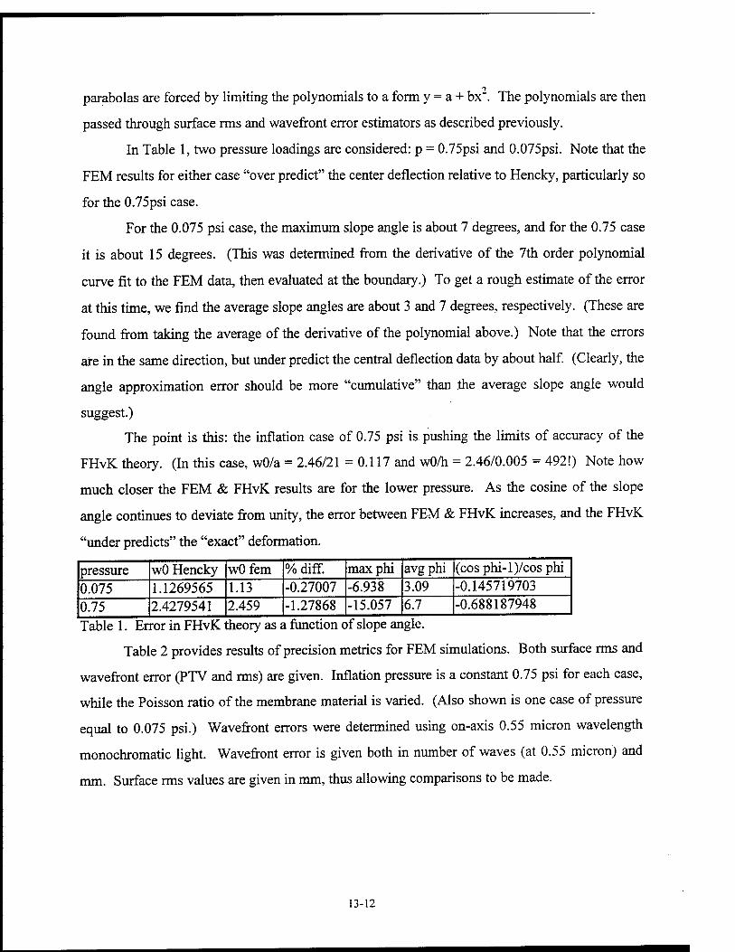
parabolas are forced by limiting the polynomials to a form y = a + bx". The polynomials are then
passed through surface rms and wavefront error estimators as described previously.
In Table 1, two pressure loadings are considered: p = 0.75psi and 0.075psi. Note that the
FEM results for either case "over predict" the center deflection relative to Hencky, particularly so
for the 0.75psi case.
For the 0.075 psi case, the maximum slope angle is about 7 degrees, and for the 0.75 case
it is about 15 degrees. (This was determined from the derivative of the 7th order polynomial
curve fit to the FEM data, then evaluated at the boundary.) To get a rough estimate of the error
at this time, we find the average slope angles are about 3 and 7 degrees, respectively. (These are
found from taking the average of the derivative of the polynomial above.) Note that the errors
ate in the same direction, but under predict the central deflection data by about half. (Clearly, the
angle approximation error should be more "cumulative" than the average slope angle would
suggest.)
The point is this: the inflation case of 0.75 psi is pushing the limits of accuracy of the
FHvK theory. (In this case, wO/a = 2.46/21 = 0.117 and wO/h = 2.46/0.005 = 492!) Note how
much closer the FEM & FHvK results are for the lower pressure. As the cosine of the slope
angle continues to deviate from unity, the error between FEM & FHvK increases, and the FHvK
"under predicts" the "exact" deformation.
pressure wO Hencky wOfem % diff. max phi avgphi (cosphi-l)/cosphi 0.075 1.1269565 1.13 -0.27007 -6.938 3.09 -0.145719703 0.75 2.4279541 2.459 -1.27868 -15.057 6.7 -0.688187948 Table 1. Error in FHvK theory as a function of slope angle.
Table 2 provides results of precision metrics for FEM simulations. Both surface rms and
wavefront error (PTV and rms) are given. Inflation pressure is a constant 0.75 psi for each case,
while the Poisson ratio of the membrane material is varied. (Also shown is one case of pressure
equal to 0.075 psi.) Wavefront errors were determined using on-axis 0.55 micron wavelength
monochromatic light. Wavefront error is given both in number of waves (at 0.55 micron) and
mm. Surface rms values are given in mm, thus allowing comparisons to be made.
13-12
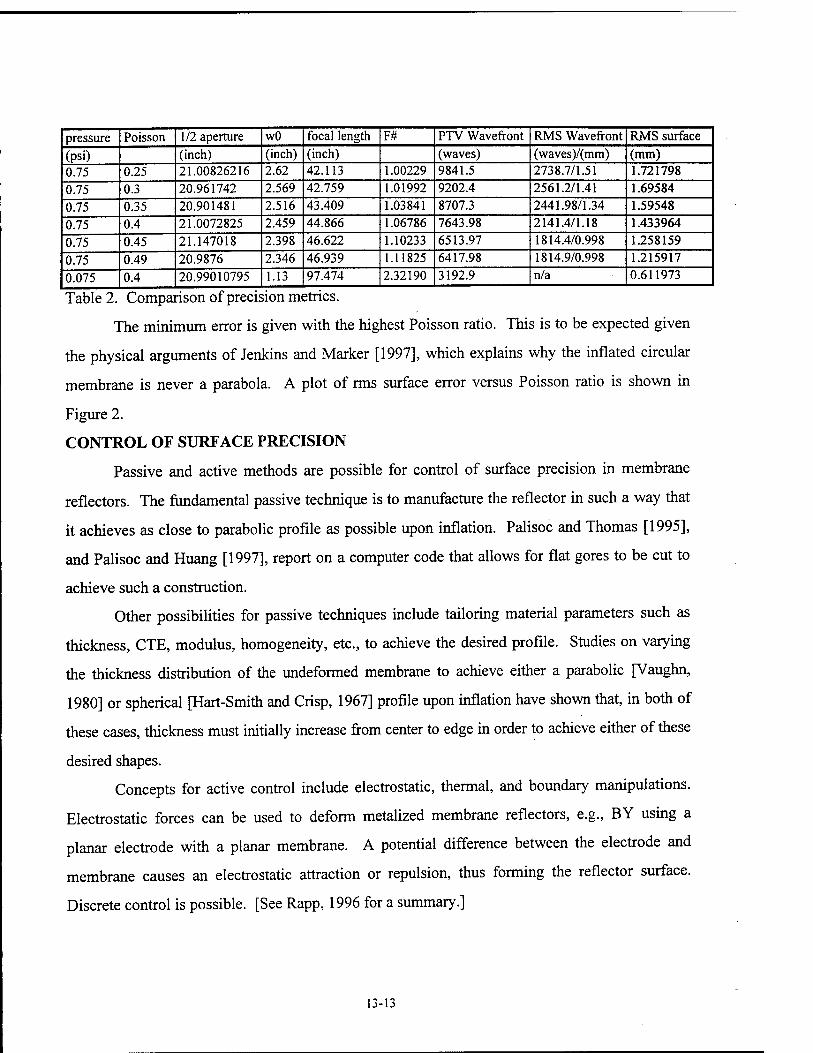
pressure Poisson 1/2 aperture wO focal length F# PTV Wavefront RMS Wavefront RMS surface
(psi) (inch) (inch) (inch) (waves) (waves)/(mm) (mm) 0.75 0.25 21.00826216 2.62 42.113 1.00229 9841.5 2738.7/1.51 1.721798
0.75 0.3 20.961742 2.569 42.759 1.01992 9202.4 2561.2/1.41 1.69584
0.75 0.35 20.901481 2.516 43.409 1.03841 8707.3 2441.98/1.34 1.59548
0.75 0.4 21.0072825 2.459 44.866 1.06786 7643.98 2141.4/1.18 1.433964
0.75 0.45 21.147018 2.398 46.622 1.10233 6513.97 1814.4/0.998 1.258159
0.75 0.49 20.9876 2.346 46.939 1.11825 6417.98 1814.9/0.998 1.215917
0.075 0.4 20.99010795 1.13 97.474 2.32190 3192.9 n/a 0.611973
Table 2. Comparison of precision metrics.
The minimum error is given with the highest Poisson ratio. This is to be expected given
the physical arguments of Jenkins and Marker [1997], which explains why the inflated circular
membrane is never a parabola. A plot of rms surface error versus Poisson ratio is shown in
Figure 2.
CONTROL OF SURFACE PRECISION
Passive and active methods are possible for control of surface precision in membrane
reflectors. The fundamental passive technique is to manufacture the reflector in such a way that
it achieves as close to parabolic profile as possible upon inflation. Palisoc and Thomas [1995],
and Palisoc and Huang [1997], report on a computer code that allows for flat gores to be cut to
achieve such a construction.
Other possibilities for passive techniques include tailoring material parameters such as
thickness, CTE, modulus, homogeneity, etc., to achieve the desired profile. Studies on varying
the thickness distribution of the undeformed membrane to achieve either a parabolic [Vaughn,
1980] or spherical [Hart-Smith and Crisp, 1967] profile upon inflation have shown that, in both of
these cases, thickness must initially increase from center to edge in order to achieve either of these
desired shapes.
Concepts for active control include electrostatic, thermal, and boundary manipulations.
Electrostatic forces can be used to deform metalized membrane reflectors, e.g., BY using a
planar electrode with a planar membrane. A potential difference between the electrode and
membrane causes an electrostatic attraction or repulsion, thus forming the reflector surface.
Discrete control is possible. [See Rapp, 1996 for a summary.]
13-13
Application of temperature gradients to the reflector may be used to effect changes in the
surface profile. Haftka and Adelman [1985] investigated such a scheme analytically for large
space structures. Selective heating of the membrane surface via a laser is an intriguing
possibility.
Manipulating the boundary (rim) of the reflector has been shown in simulations to be
effective. Jenkins [1996], Jenkins and Marker [1997], and Marker and Jenkins [1997] have
shown that the figure error in the inflated membrane profile can be reduced through judicious
boundary displacements [see also Natori et al., 1989].
REFERENCES
Cambell, J.D. (1956), "On the theory of initially tensioned circular membranes subjected to
uniform pressure," Q JMech Appl Math 9, 84-93.
Chien, W.Z. (1948), "Asymptotic behavior of a thin clamped plate under uniform normal pressure
at very large deflection," Sei. Rep. Natn. TsingHua Univ. A5, 71-94.
Dickey, R.W. (1967), "The plane circular elastic surface under normal pressure," Arch Rational
Mech Anal 26,219-236.
Fichter, W. B. (1984), "Reduction of root-mean-square error in faceted antennas," AIAA J 22,
1679-1684.
Fichter, W. B. (1997), "Some solutions for the large deflections of uniformly loaded circular
membranes," NASA Technical Paper 3658.
Föppl, A. (1907), "Vorlesungen über technische Mechanik," B.G. Teubner, Bd. 5., p. 132, Leipzig,
Germany.
Haftka, R. T., and Adelman, H. M. (1985), "An analytical investigation of shape control of large
space structures by applied temperatures," AIAA J23, 450-457.
Hart-Smith, L.J., and Crisp, J.D.C. (1967), "Large elastic deformations of thin rubber membranes,"
Int J Eng Sei 5,1-24.
Hedgepeth, J.M. (1982), "Accuracy potentials for large space antenna reflectors with passive
structures," J Spacecraft 19(3), 211-217.
Hencky, H. (1915), "Über den Spannungszustand in kreisrunden Platten," Z Math. Phys. 63, 311-
317.
Jeffreys, H., and Jeffreys, B. S. (1972), Methods of mathematical physics, Cambridge.
13-14

Jenkins, C.H., Marker, D.K., and Wilkes, J.M. (1998a), "Improved surface accuracy of precision
membrane reflectors through adaptive rim control," AIAA Adaptive Structures Forum, Long
Beach, CA (to appear).
Jenkins, C.H., Wilkes, J.M., and Marker, D.K. (1998b), "Surface accuracy of precision membrane
reflectors," Space 98, Albuquerque, NM (to appear).
Jenkins, C. H., and Marker, D. K. (1997), "Surface precision of inflatable membrane reflectors,"
JSolar Energy Engr (in review).
Jenkins, C.H. (1996). Shape Control of an Inflated Membrane Disk: Preliminary
Investigation. Summary Report, Phillips Laboratory, Kirtland AFB.
Jenkins, C.H. (1996), "Nonlinear Dynamic Response of Membranes: State of the Art -
Update," ApplMech Rev 49 (10), S41-S4S.
Jenkins, C.H., and Leonard, J.W. (1991), "Nonlinear Dynamic Response of Membranes:
State of the Art," Appl Mech Rev 44, 319-328.
Kao, R., and Perrone, N. (1971), "Large deflections of axisymmetric circular membranes," Int J
Solids Struct 1,1601-1612.
Kao, R., and Penone, N. (1972), "Large deflections of flat arbitrary membranes," Comput Struct 2,
535-546.
Libai, A. and Simmonds, J.G. (1988), "The nonlinear theory of elastic shells," Academic Press.
Marker, D. K., and Jenkins, C. H. (1997), "On the systematic "W" profile error in
uncompensated isotropic membrane reflectors," 25th Midwestern Mechanics Conf, Rapid
City, SD.
Meyer, R. X. (1985), " Precision of mesh-type reflectors for large space-borne antennas," J
Spacecraft 22,80-84.
Mikulus, M. M. (1964), "Behavior of a flat stretch membrane wrinkled by the rotation of an
attached hub, NASA Technical Note TND-2456.
Miller, R. K., Hedgepeth, J. M., Weingarten, VI, Das, , and Shahrzad K. (1985), "Finite element
analysis of partly wrinkled membranes," Computers Structures 20, 631-639.
Murphy, L.M. (1987), "Moderate axisymmetric deformations of optical membrane surfaces," J
Solar Energy Eng 109,111-120.
13-15
Murphy, L.M. (1986), "Stretched-membrane heliostat technology," J Solar Energy Eng 108, 230-
238.
Natori, M., Shibayam, Y., and Sekine, K. (1989), "Active accuracy adjustment of reflectors
through change of element boundary," AIAA paper no. 89-1332-CP.
Palisoc, A., and Thomas, M. (1995), "A comparison of the performance of seamed and
unseamed inflatable concentrators," Solar Engineering 1995:1995 ASME/JSME/JSES Int
Solar Energy Con/2, 855-864.
Palisoc, A. L., and Huang, Y. (197), "Design tool for inflatable space structures," AIAA paper
97-1378.
Press, W. H., Flannery, B. P., Teukolsky, S. A., and Vetterling, W. T. (1986), Numerical
recipes, Cambridge Univ. Press.
Rapp, D. (1996), "Prospects and limitations of technical approaches for ultra lightweight space
telescopes," JPL Report D-13975.
Ruze, J. (1966), "Antenna tolerance theory - a review," Proc. IEEE 54, 633-640.
Schmidt, R. (1974), "On Berger's method in the non-linear theory of plates," JAppl Mech 41, 521-
523.
Schmidt, R., and DaDeppo, D.A. (1974), "A new approach to the analysis of shells, plates, and
membranes with finite deflections," Int J Non-Linear Mech 9,409-419.
Shaw, F.S., and Perrone, N. (1954), "A numerical solution for the non-linear deflection of
membranes," JAppl Mech 21,117-128.
Shortal, J. A. (1978), "A new dimension: Wallops Island flight test range - the first fifteen
years," NASA Reference Publication 1028.
Stevens, H.H. (1944), "Behavior of circular membranes stretched above the elastic limit by air
pressure," Experimental Stress Analysis 2,139-146.
Stein, M, and Hedgepeth, J. M. (1961), "Analysis of partly wrinkled membranes, NASA Technical
Note D-813.
Storakers, B. (1983), "Small deflections of linear elastic circular membranes under lateral
pressure," JAppl Mech 50, 735-739.
Thomas, M., and Veal, G. (1984), "Highly accurate inflatable reflectors," AFRPL TR-84-021.
13-16
Vaughn, H. (1980), "Pressurizing a prestretched membrane to form a paraboloid," IntJEng Sei 18,
99-107.
von Kärmän, T. (1910), "Festigkeitsproblem im Naschinenbau," Encyk D Math Wiss IV, 311-385.
Walker, B. H. (1994), Optical engineering fundamentals, McGraw-Hill.
Weil, N.A., and Newmark, N.M. (1955), " Large plastic deformations of circular membranes," J
ApplMech 22, 533-538.
Wilkes, J.M. (1997), private communication.
Zarghamee, M.S. (1967), "On antenna tolerance theory," IEEE Trans Antennas Propagat. AP-
15,777-781.
13-17
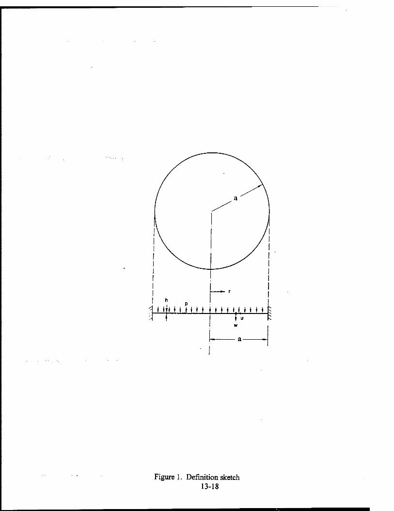
h
n(mtm j u M,m H TT ♦
a-
Figure 1. Definition sketch 13-18
u CO
o CO co
• 1—1 o
ejoqe.red:iii9j 6(mm) IOJJQ aoejins suu Figure 2. RMS surface error vs. Poisson's ratio.
13-19
MODE CONVERSION IN A TIME-VARYING MAGNETOPLASMA MEDIUM
Dikshitulu K. Kalluri Professor
Department of Electrical Engineering
University of Massachusetts Lowell One University Avenue
Lowell, MA, 08154, USA
Final Report for: Summer Faculty Research Program
Philips Laboratory / Geophysics Directorate
Sponsored by: Air Force Office of Scientific Research
Boiling Air Force Base, DC
and
Phillips Laboratory /Geophysics Directorate
September 1997
14-1
Mode Conversion in a Time-varying Magnetoplasma Medium
Dikshitulu K. Kalluri Professor
Department of Electrical Engineering University of Massachusetts Lowell
Lowell, MA, 08154, USA
Abstract
The modification of frequency and field amplitudes of an extraordinary wave (X wave) by a time-varying
magnetoplasma medium is considered. An explicit expression for the amplitude of the electric and magnetic fields in
terms of the magnetoplasma parameters and the new frequency is obtained. Based on the qualitative results, one
many conclude that the mode conversion takes place in the neighborhood of CO b « CO 0 .
14-2
Mode Conversion in a Time-varying Magnetoplasma Medium
Dikshitulu K. Kalluri
I. Introduction
The main effect of switching a magnetoplasma[l-17] is the splitting of the source wave into new waves
whose frequencies are different from the frequency of the source wave. When the medium properties change slowly
with time due to slow change of the electron density in the plasma, one of these waves whose initial frequency is the
source frequency will be the dominant new wave in the sense that its field amplitudes will be significant. Other
waves have field amplitudes of the order of the initial slope of the electron density profile. The case of longitudinal
propagation is already discussed in [13, 16-17]. The case of transverse propagation involving X-waves[18] is the
topic of this report. A more complete account of this research will be published elsewhere [19].
II Transverse Propagation
II. 1 Development of the problem
The geometry of the problem is shown in Figure 1. Initially, for time t < 0, the entire space is considered
to be free space. A uniform electromagnetic plane wave with a frequency CO 0 propagating in the positive z direction
and the electric field in the positive x direction is established over the entire space.
The fields of the source wave are given by:
E(z,t) = xE0eji(0"'-k"z\ r<0, (la)
U(z,t) = yH0eAo,"'-k"z), t<0, (lb)
where k0 is the free space wave number, E0 =X[0H0, V\0 is the intrinsic impedance of free space, and
/ = V- 1 • A static magnetic field B0 is present along the ^-direction.
At time / = 0, the entire space is converted into a time varying plasma medium. The plasma medium is
spatially homogeneous and unbounded. Therefore the wave number k0 remains constantfl]. The free electron
density N(t) is slowly increasing to a certain value N0 with zero initial value. Therefore the plasma medium has
a time-varying plasma frequency CO (/) and an electron gyrofrequency CO b given by
©6=—, (2b) m
14-
where q is the absolute value of Othe charge, m the mass of the electron, and B0 the magnitude of B0. With these
assumptions, we can write the fields for / > 0 as follows:
E(z,t) = [xEx(t) + zE2(t)yß"\ t>0, (3a)
H(z,t) = yHy(t)e-Jk°z, t>0, (3b)
\(z,t) = [xvx(t) + zvz{t)YJk"\ t>0, (3c)
where v(z, t) is the velocity of an electron. The differential equations for these fields can be obtained by using the
Maxwell equations:
dU VxE = -^0—, (4a)
ot
5E VxH-s0 — + J. (4b) 0 dt
From (3) and (4) the following differential equations are obtained:
ot
^ = j(o0J\0Hv- — Jx, (5b) dt ■ s0
dE 1 —?- = —J_. (5c) dt S0 '
Here Jx and J, denote the current density components. The current density vectors are closely related to the
motion of the electron charges.
II.2 Current Density Vector
In the previous section, we obtained three equations with five unknowns. Two more equations are needed
to determine the five unknowns. The equation of motion of the electrons is given by the Lorentz force equation:
dx_
dt
The velocity vector may be related to the current density vector. When free space is slowly converted into plasma, it
is necessary to impose the requirement that the electrons born at different times have zero initial velocity [12-13].
Applying these concepts to the case of transverse propagation [14] we obtain the equations for Jx and Jz given
below:
- = en<o-„Ex +<£>„JZ, (7a)
m— = -g|E + vxB0J. (6)
dt '" " x
14-4
Q- = z0<ü20E-(übJx. (7b) dt ° p
11.3 Higher order differential equation
Equations (5) and (7) are the first order coupled differential equations that contain time-varying and
complex coefficients. Generally, it is difficult to obtain exact solutions, but reasonable approximate solutions can be
obtained. Equations (5) and (7) are manipulated by differentiation and substitution and a fifth order differential
equation for E is obtained:
EXS) + AEf + BE? + g[5Ex
2) + (2co; + 3co2 )£ J +
de d2g (8)
dtx x " z dt1
where
^ = co;+2co;+co^. (9a)
5 = ©>;+(ö>;+a>J. (9b)
d®2
a = dt
P (9c)
A /i2
We neglect —, —7-, and g2 since C02(0 is a slowly varying function of time. The equation for Ex becomes dt ' dt' p
simpler and is given by:
E{? + AE? + BE? + g[5Ex2*> +(2co2 +3co2 )EX] = 0. (10)
11.4 Riccati equation
To solve (10), the WKB method can be applied [15]. A complex instantaneous frequency function, /?(/),
is defined such that
dEr
dt = p(t)Ex. (ID
Then
E™=(P + P2)EX, (12a)
Ex3)=(p + 3pp + p3)Ex, (12b)
Ef =(p + App + 6p2p + 3/r + pA)Ex, (12c)
E[S) = [(pw + 5pp + \0(p + p2)p + 5(2/ + 3pp)p + ps)]Ex. (I2d)
Substitution of (12) into (10) gives 14-5
p{A) + 5pp +10(p + p2 )p + 5(2 p3 + 3pp)p + p5 +
A(p + 3pp + p3)+Bp + g[5(p + p2) + (2a2o+3(a2
p)] = 0:
This Riccati equation can be solved to zero order and the solution gives real frequencies of the new waves.
II.5 Frequencies of the new waves
We let p = j(0 in (13) and neglect higher order terms (p, p, p , pW, g, and their powers), then we
get
co5 - Aco3 + B(ü = 0. (14)
The solutions to this equation can be easily obtained as
for©6<C0o,
' ", (15a)
(15b)
(15c)
(15d)
C05=0, (15e)
for CO, >C0„,
CO,- -JA1- -45
co2 -4 A2 -AB
co3 = -co,,
co4 = -co2,
CO,
CO-
= [±{A-jA2-4B}f, (16a)
[±{A + jA2-4B}f, (16b)
C03=-CO,, (16c)
co4 = -co2, (16d)
C05 = 0. (16e)
We split the solutions into two regions given by (15) and (16) to obtain the same initial values at / = 0.
Consequently, in both regions, the first wave has the same initial value CO 0 and may be considered as the modified
source wave (MSW). The other waves may be considered as new waves created by the switching action and are of
the order of g(0) = g0. Equations (15) and (16) are the same as those that can be obtained from the consideration
of conservation of the wavenumber of the X wave in a time-varying, unbounded, and homogeneous plasma medium
[15].
Equations (15) and (16) show that five new waves are generated when t > 0 as a result of the imposition of
the magnetoplasma. The first two solutions are transmitted waves while the next two are reflected waves. Since CO 5
is zero, the fifth solution is not a wave.
14-6
11.6 Amplitudes of the Fields of the New Waves
Amplitudes of the fields of the new waves can be obtained by expanding the frequency function to include a
real part. Let p - a + ja . Neglecting higher order terms except a ,ob , and g, we can get the relation for a :
g(5co2„-2co^-3co2p)-cu(10a)2n-3^)con
a"" 5co^-3^©; + 5 '
11.7 Complete Solution
The complete solutions to the problem can be represented by the linear combination of the five new modes.
Let's suppose the field components have the following form:
Ex =Eet ^exp[£(y<Dll(T) + a1I(T))rfc]. (18)
To determine the unknown coefficients An, we can use the initial conditions at t = 0.
Ex(0)=Eo, (19a)
£z(0) = 0, (19b)
Hy(0)=Ho, (19c)
J,(0) = 0, (19d)
Jr(0) = 0. (19e)
Symbolic manipulations [20] have been done to obtain the coefficients:
. co4A+14co2(Q2+co^
4=1- JSo 0„ ,„2 „2,3 > (20a)
®h A _ ,-p. rl* (20b) 2 ^°2(CO0+CDA)K-CDA)
3'
A =-io — 7 (20d) 4 ^O2(co0-co6)((o0+oj3'
^5 = 0. <20e)
The above expressions become singular when C0o = C0A. The evaluation of the unknown constants using (18)
makes it possible to describe the transmitted fields and the reflected fields completely in terms of their time-varying
envelope functions and the frequency functions. The resulting expression is
Ex(z,t)=E0fdAnexp\ßn(t)]expU(Qn(t)-k0z)], (21)
14-7
where
e„(0=K(Tyt.
ß„(0=K(xVx.
(22a)
(22b)
II.7 Explicit Expressions for the Amplitudes of the Fields
The expression for g in terms of CD may be obtained by differentiating (14):
g = 2(2co2-;Qcocb
2co2-co2-2co27
From (17) and (23), a(t) can be expressed as
(CO2.4-2(2CO2+CO>2)Cü 2coco; co; «(0 = co -■
2CO(2Cö2Cö2^3CO>2+CO*+2Cü2Cö2) G(G-co2) 2coG CO .
where
G = A/4CO2CO2 -4co2 1
+ <
K = (2co2- <- G) /2.
We can integrate (24) to obtain ß(0 :
Mrt - f 1
n(T\r!r — ——Inf G- 1 N IT» \ A- :
ö>6 In G + Vco'-4co2co2
•4co2co2 CO
(0(0
(o(0)
(23)
(24)
(25a)
(25b)
(26)
II. 8 Adiabatic Analysis of the Modified Source Wave
For the first wave, from (26),
F(0 = exp[ß,(0] = G>;-G>;
2cof-co2-2co2-co2
CO 0 2co2-co2-2co2+Vco^-4co2co:
vco,
l^-W^l
(27)
In (27) the factors including the last exponent are real for CO" > 4(H'b . For other ranges, some of these factors are
complex but easily computed by using mathematical software [15]. For small g0 , and coo sufficiently different
from CO b. A] =1 and the other A coefficients are negligible. Only the first wave has significant amplitude and it
14-8
may be labeled as the Modified Source Wave (MSW). Each of the fields' of the MSW may be written as a product of
an instantaneous amplitude function and a frequency function:
Ex(z,t) = E0ex(t)cos[Q](t)-k0z],
Hy{z,t) = H0hy(t)co{Qx(t)-k0z],
Ez{z,t) = E0e2(t) cos 0,(0 -k0z + - 71
where the instantaneous amplitude functions are given by
ex(t) = F(t),
<ö.
y ©,(/)
e,(0 = ©*«;
©,(/)[©,(o-«;(0-«; and the power density function S(t) is given by
F(0,
S('^itr^ For co6« C0o the amplitude functions reduce to
<?,(') = co;
W*+CDJ(0,
2co;(co;+co2p(o)ln
CO,
1+- to„+co;(/)y
-or,(o(3co2+2co2(o) co;
4co:(co2+co;(0)
(28a)
(28b)
(28c)
(28d)
(28e)
(28f)
(29)
(30a)
^(0 = CO.
.co2.+<(')/
< © *»;(/)
^l^l+^liO
For CO,» CO „ and CO h» CO ,
ex(t) = l
ez(0 =
3co;(Q
4 co2,
co;(0
»ft^o
(30b)
(30c)
(30d)
Graphical results given in Section III are obtained by computing F(l) from (27). The results are verified using
(22b) involving a numerical integration routine.
14-9
HI Graphical Illustrations and Results
An exponentially varying electron density profile is used for an illustrative example. The time-varying
plasma frequency is considered as:
coJ(0 = <[l-exp(-Z>0]- (3D
The results for the first wave are presented in a normalized form by taking CO 0 — 1. The parameter b is
chosen as 0.01. Figures 2, 3, and 4 show the characteristics of the MSW. It has an upshifted frequency (Fig. 2)
compared to the source wave frequency CO 0 when CO b < CO 0 and a downshifted frequency when CO b > CO 0 . The
amplitude function ex(t) (Fig. 3) of the MSW decreases with the increase of (£>b as long as C0A < C0o. However, it
increases with C0A for (£>b >C00 . The amplitude function h (t) follows a similar pattern. The amplitude function
e,{t) changes sign as (Hb value crosses (S$b = C0o (Fig. 4).
Figures 5, 6, 7, and 8 show the variation of the saturation values (/ —> oo) of the frequency and amplitude
function of the MSW. The horizontal axis is CO b. However, in the neighborhood of CO b « CO 0 , the assumptions
Ax « land all other A's are zero are not valid. The following validity condition is obtained by restricting the
magnitude of the second term on the right hand side of (20a) to be less than 0.1. The validity condition is
-> co:
>
( KV/3 20-^-
V ®o J (32)
From Figures 5-8, the following qualitative result may be stated: as the value of CO b crosses CO 0, there will be a
rapid change in the frequency and the fields of the source wave, signifying a mode conversion.
IV Conclusion
The creation of a time varying magnetoplasma medium splits the incident wave into four new waves having
different frequencies in the case of transverse propagation. Two of the waves are transmitted waves and the other
two are the reflected waves. The first wave whose initial frequency is that of the incident wave has the strongest
intensity compared to the others and is labeled as the MSW. Based on the adiabatic analysis of the MSW, the
following qualitative statement may be made: as the value of CO b crosses CO 0 , there will be a rapid change in the
frequency and the fields.
We still have difficulty in quantifying the behavior of the fields in the neighborhood of CO b » CO 0 . The
accuracy of the solution degrades since CO at t = 0 tends to infinity as CO b tends towards CO 0. In this
neighborhood the higher order terms become important. The aspect of the effect at CO b = CO 0 is currently under
investigation using a very different approach and the result will be reported in due course.
14-10

Adiabatic solutions given in this paper can give explicit analytical description for the frequency and the
amplitude of the modified source wave except in the neighborhood of ©A ~ coo . Based on the qualitative results,
one many conclude that the mode conversion takes place in this neighborhood
References
[I] C. L. Jiang, "Wave propagation and dipole radiation in a suddenly created plasma," IEEE Trans. Antennas
Propagat., vol. AP-23, no. 1, pp. 83-90,1975
[2] D. K. Kalluri, "On Reflection from a Suddenly Created Plasma Half-Space: Transient Solution," IEEE Trans.
Plasma Sei., vol. 16, no. l,pp. 11-16,1988
[3] V. R. Goteti and D. K. Kalluri, "Wave Propagation in a Switched-on Time-varying Plasma Medium," IEEE
Trans. Plasma Set, vol. 17, pp. 828-833, 1989.
[4] D. K. Kalluri and V. R Goteti, "Frequency Shifting of Electromagnetic Radiation by Sudden Creation of a
Plasma Slab," J. Appl. Phys., vol. 72, no. 10, pp. 4575-4580, 1992.
[5] C. J. Joshi, C. E. Clayton, K. Marsh, D. B. Hopkins, A. Sessler, and D. Whittum, "Demonstration of the
Frequency Upshifting of Microwave Radiation by Rapid Plasma Creation," IEEE Trans. Plasma Sei., vol. 18,
no. 5, pp. 814-818, 1990.
[6] S. P. Kuo and A. Ren, "Experiment Study of Wave Propagation Through a Rapidly Created Plasma," IEEE
Trans. Plasma Sei., vol. 21, no. 1, pp. 53-56, 1993.
[7] D. K. Kalluri, V. R. Goteti, "Damping Rates of Waves in a Switched Magnetoplasma Medium: Longitudinal
Propagation," IEEE Trans. Plasma Sei., vol. 18, no. 5, pp. 797-801, 1993.
[8] V. R. Goteti and D. K. Kalluri, "Wave Propagation in a Switched Magnetoplasma Medium: Transverse
Propagation," Radio Science, vol. 25, no. 1, pp. 61-72, 1990
[9] S. R. V Madala and D. K. Kalluri, "Frequency Shifting of a Wave Traveling in an Isotropie Plasma Medium
due to Slow Switching of a Magnetic Field," Plasma Sources Sei. Technol, vol. 1, pp. 242-248, 1992
[10] S. R. V. Madala and D. K. Kalluri, "Longitudinal Propagation of Low-frequency Waves in a Switched
Magnetoplasma Medium," Radio Science, vol. 28, no. 2, pp. 121-129, 1993.
[II] C. H. Lai, T. C. Katsouleas, "Frequency Upshifting by an Ionization Front in a Magnetized Plasma," IEEE
Tram. Plasma Sei., vol. 21, no. 1, pp. 45-51, 1993.
[12] A. Bafios, Jr., W. B. Mori, and J. M. Dawson, "Computation of the Electric and Magnetic Fields Induced in a
Plasma Created by Ionization Lasting a Finite Interval of Time," IEEE Trans. Plasma Sei., vol. 21, no. 1, pp.
57-69,1993
[13] D. K. Kalluri, V. R. Goteti, and A. M. Sessler, "WKB Solution for Wave Propagation in a Time-Varying
Magnetoplasma Medium: Longitudinal Propagation," IEEE Trans. Plasma Sei., vol. 21, no. 1, pp. 70-76,
1993.
14-11
114] J. H. Lee, "Wave Propagation in a Time-Varying Switched Magnetoplasma Medium: Transverse
Propagation", M.S. Thesis, University of Massachusetts Lowell, 1994.
[15] D. K. Kalluri, "Frequency Shifting Using Magnetoplasma Medium: Flash Ionization," IEEE Trans. Plasma
Sei., vol. 21, no. 1, pp. 77-81, 1993
[16] D. K. Kalluri, "Conversion of a whistler wave into a controllable helical wiggler magnetic field," J. Appl.
Phys., vol. 79, no. 9, pp. 6770-6774, 1996.
[17] D. D. Kalluri, "Frequency upshifting with power intensification of a whistler wave by a collapsing plasma
medium," J. Appl. Phys., vol. 79, no. 8, pp.3895-3899, 1996.
[18] M. A. Heald and C. B. Wharton, Plasma Diagnostics with Microwaves, New York: Wiley, 1965, p. 36.
[19] Joo Hwa Lee and D. K. Kalluri, "Modification of an Electromagnetic Wave by a Time-varying Switched
Magnetoplasma Medium: Transverse Propagation," IEEE Trans. Plasma Sei., Feb. 1998 Issue.
[20] N. Blachman, Mathematical A Practical Approach, Prentice Hall, Englewood Cliffs, New Jersey, 1992
14-12
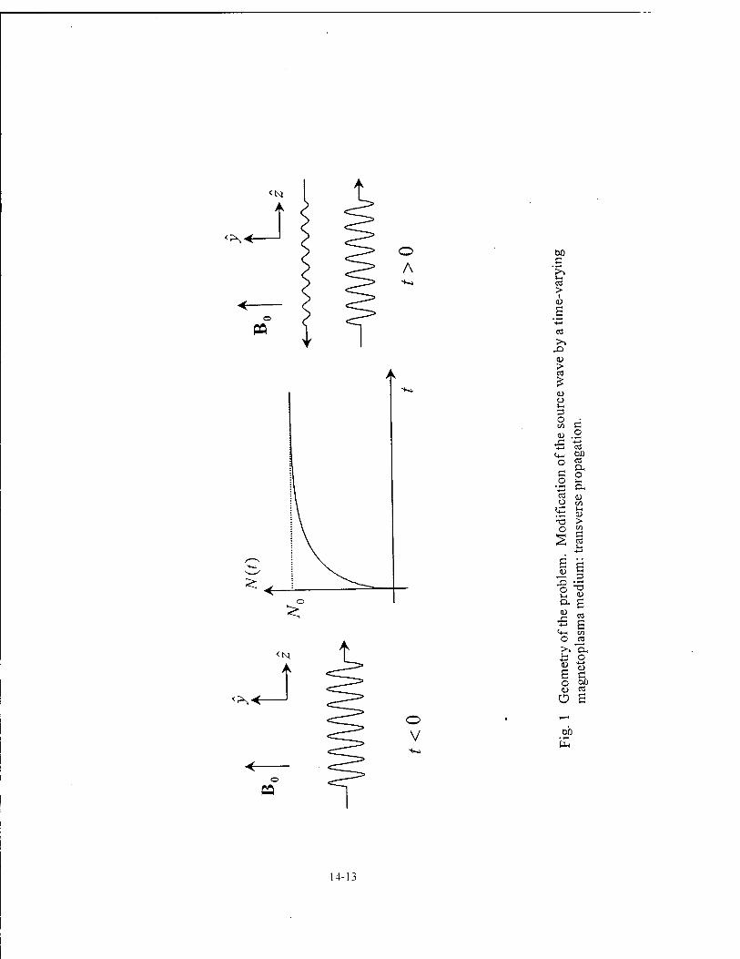
<>><- o A
«
A
<?s<-
o V
M c >. l-l cS > <u a -*-» CO
(1) > CO
£ <u o lH
3 O c/i 1-1 <L> o
■*-» CO Cl—1 ÖÜ o CO
ti. Ul O o t-<
"■+-» u, CO (1) o en C *r) > O CO
S l-l OS
-*-»
s 3
O T3 4)
OH s 4->
co
<+-! <*> o CO >* fX VH o
o DU <1> CO
Ü s *-< oil
UH
o
14-13
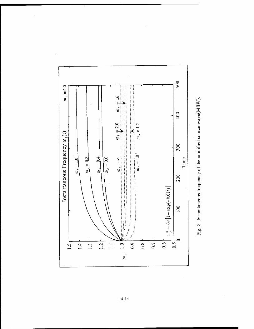
00
> CO
o l-H
o CO
T3 CD
'S -3 o g (D
o C <u cr 0)
CO
o c
C C3
ob
14-14
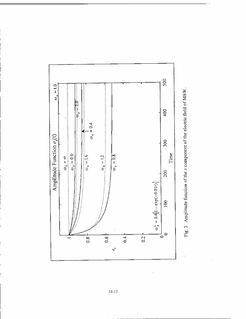
t/3
o
o
o
(D
C C o
o o
J3
c .2 o ,3 -t—I
ID X)
S <
E
14-15
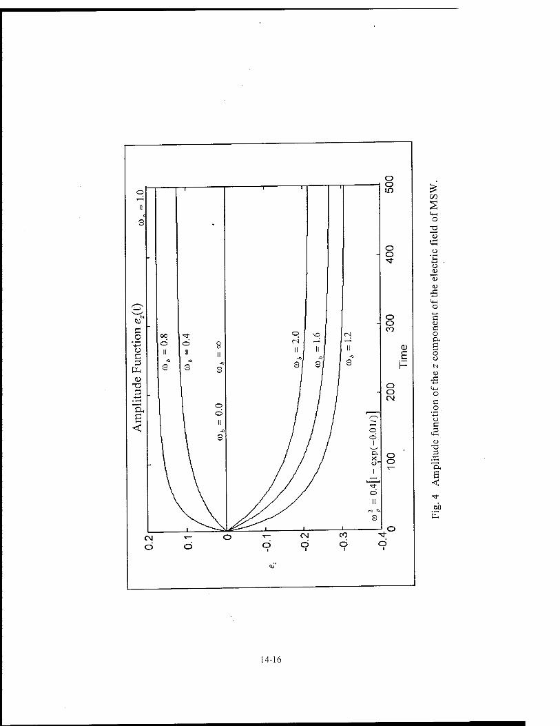
00
o
ml o
o
«-«—I
o e
o
£ o o N
Ö o o e
<L) •o
"a, S
ob tu
14-16
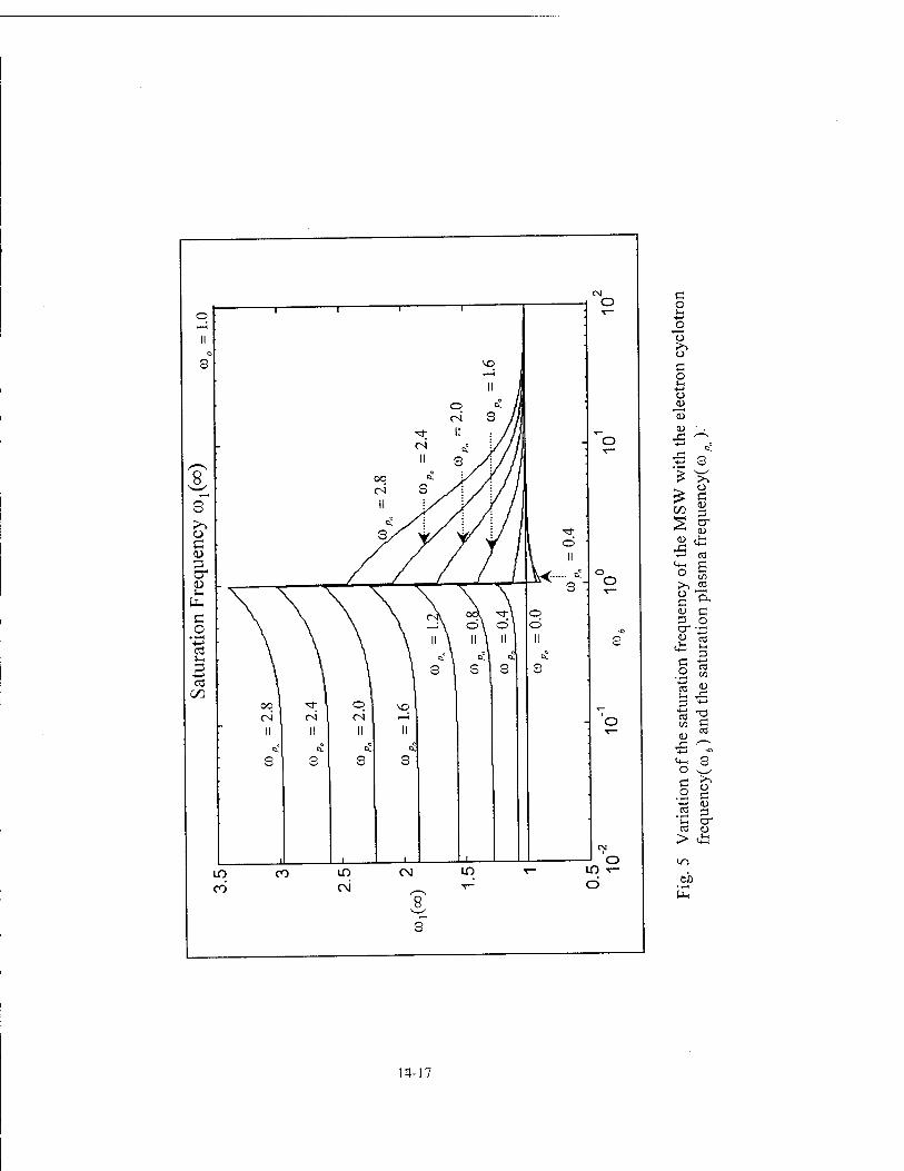
c o i-*
+-> o o >% o c o t-l
■*-»
o (!) <u 0)
XI ^"^ -4—» - = X R £ >-.
00 1
2 <1>
X! »'-' <+-<
•+-» 03 tu o B o c ex <u c 3 o cr (L) rrt
'M S-H 3
C o CO
(D I-i
3 4-J
T3 t/1 Ü
m <1) X '^^ -4-»
<+H S Ü
o >> o c -*-» l\>
CO 3 i-. rr 03 (1)
> l/~)
M
U-.
14-17
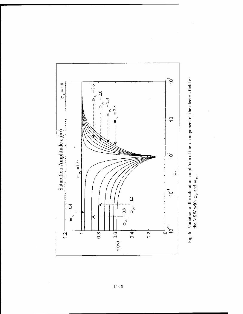
CM
o o 1 i i 1
,"H
II II o
s s ii
1 3 CN
II 00 cj <N
3 « c£ _ "o
3 ^
IT X. w
(D <^y "Ö 3 -(->
. o o
s o : T—
< o
c II o - -c
• ^* CL s to 3 s- 3 +J cö
oo 'o T—
CN ^
■<*■ <••■•
II Ö oo ^
II ; ► © 3 . s£
<■■- .11
s
j
3
c Nl v- CO CD ^ CM O T-
Ö Ö Ö Ö
o
is
X
o c <u c o a, B o o K
<+-t o
3
o 3 -*-» m -a
!-i 3 ca
4—J
CO -c I/J 3 <1> r-; XI
-t—»
o £ a £
f/> CO s t- ai (LI
> X -4—»
\o OX)
PH
14-18

o
is o '£ Ü
c c o a, o
o
3
a, £ CO
C .2 |3
£ S <4-H
o .C
2 £ :«£ > S
.2?
14-19
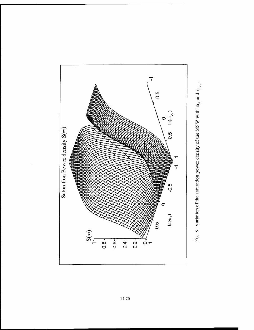
S3 es
S
C0
o
1/1 Ö
u
o a, Ö
1-1
en <D
J3
o
> oo ob
14-20
MEASUREMENT OF THE CUTTING PERFORMANCE OF A HIGH BEAM QUALITY CHEMICAL OXYGEN-IODINE LASER OF AEROSPACE AND
INDUSTRIAL MATERIALS
Aravinda Kar Associate Professor
Department of Mechanical and Aerospace Engineering
University of Central Florida P.O. Box 162700
Orlando, FL 32816-2700
Final Report for: Summer Research Program
Phillips Laboratory
Sponsored by: Air Force Office of Scientific Research
Boiling Air Force Base, Washington, DC
And
Phillips Laboratory
July, 1997
15-1
MEASUREMENT OF THE CUTTING PERFORMANCE OF A HIGH BEAM QUALITY CHEMICAL OXYGEN-IODINE LASER ON AEROSPACE AND INDUSTRIAL
MATERIALS
Aravinda Kar Assistant Professor
Department of Mechanical, Materials and Aerospace Engineering Center for Research and Education in Optics and Lasers
University of Central Florida
Abstract
Chemical Oxygen-Iodine Laser (COIL) technology has received considerable interest over
the last several years due to its short, fiber-deliverable wavelength (1.315 microns), scalability to
high powers (tens of kilowatts, cw), and potentially high beam quality. Unfortunately, materials
processing demonstrations to date have been performed with relatively small COILs producing
very poor quality beams (M2 > 100). This paper documents the cutting performance of a high
beam quality COIL. Cut depth and width on a variety of materials is documented as a function of
various process parameters. Also, the optical quality of the laser beam is evaluated in this study.
15-2
MEASUREMENT OF THE CUTTING PERFORMANCE OF A HIGH BEAM QUALITY CHEMICAL OXYGEN-IODINE LASER ON AEROSPACE AND INDUSTRIAL
MATERIALS
Aravinda Kar
1. Introduction
Lasers have been successfully used for commercial cutting applications. C02 and Nd:YAG
lasers are usually used for such applications. Chemical Oxygen-Iodine Laser (COIL) is a scalable
high power laser at wavelength 1.315 urn that can be used for various types of materials
processing. Kar et al.1 briefly discussed the basic principle of COIL and demonstrated the thick-
section cutting capability of COIL. Atsuta, et al.2 showed that the cutting capability of a 1 kW
COIL is equivalent to a 1 kW Nd:YAG laser and about 2.5 times better than a 1 kW C02 laser.
They presented a simple two-parameter model and empirically determined these two parameters
by fitting the model to their experimental data in order to predict the scaled cutting capability of
COIL2.
Tikhomirov3, Schuocker4, and Powell5 summarized earlier studies on laser cutting of various
types of materials. Chryssolouris and Choi6, Biermann et al.7, and Molian and Baldwin8 examined
the effects of cutting gas jet on laser cutting. Ohlsson et al.9 compared the effectiveness of laser
and abrasive water jet cutting processes. Laser cutting of highly reflective materials such as
copper and aluminum was investigated by Thompson10. Hack et al.11 used glass fibers to deliver
Nd: YAG laser to the workpiece in the power range up to 2.3 kW to cut materials.
The interactions of various process parameters during laser cutting have also been studied by
using mathematical models. Schuocker and Abel12, and Schuocker13 analyzed the material
removal process during laser cutting. Li and Mazumder14 presented a mathematical model for
laser cutting of wood. Modest and Abakians15, Bang and Modest16, and Roy and Modest17
carried out heat transfer analysis for evaporative cutting. Belie and Stanic , and Belie used
empirical parameters to develop a simple model for laser cutting.
The purpose of this work is to investigate the cutting capability of COIL for various types of
materials such as aluminum, copper, nickel and titanium. The experimental data are also
compared with a scaling law to evaluate the accuracy of the theoretical model.
15-3
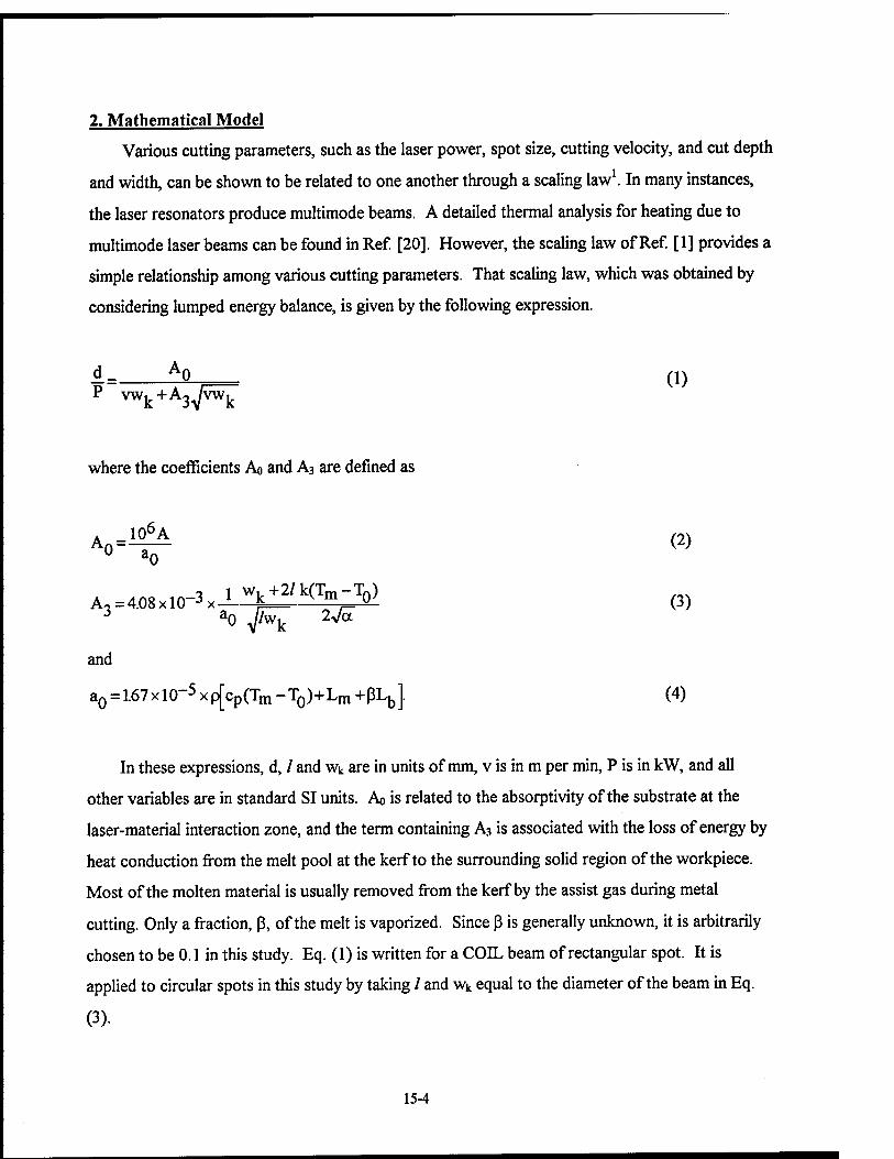
2. Mathematical Model
Various cutting parameters, such as the laser power, spot size, cutting velocity, and cut depth
and width, can be shown to be related to one another through a scaling law1. In many instances,
the laser resonators produce multimode beams. A detailed thermal analysis for heating due to
multimode laser beams can be found in Ref [20]. However, the scaling law of Ref. [1] provides a
simple relationship among various cutting parameters. That scaling law, which was obtained by
considering lumped energy balance, is given by the following expression.
AP_T= (1) P vwk+A3>/vw^
where the coefficients Ao and A3 are defined as
A0=1^A (2) 0 a0
o i w. +2/k(Tm-Tn) A, = 4.08xl0"3x-i * v m. °' (3)
a0 yjto^ 2>/a
and
aQ = 1.67xl0-5 xp[cp(Tm -T0)+Lm +ßLb]. (4)
In these expressions, d, / and wk are in units of mm, v is in m per min, P is in kW, and all
other variables are in standard SI units. Ao is related to the absorptivity of the substrate at the
laser-material interaction zone, and the term containing A3 is associated with the loss of energy by
heat conduction from the melt pool at the kerf to the surrounding solid region of the workpiece.
Most of the molten material is usually removed from the kerf by the assist gas during metal
cutting. Only a fraction, ß, of the melt is vaporized. Since ß is generally unknown, it is arbitrarily
chosen to be 0.1 in this study. Eq. (1) is written for a COIL beam of rectangular spot. It is
applied to circular spots in this study by taking / and wk equal to the diameter of the beam in Eq.
(3).
15-4
3. Experimental Procedure
A RADICL device (Research Assessment, Device Improvement »Chemical Laser) located at
the U.S. Air Force's Phillips Laboratory in Albuquerque, New Mexico, was used to carry out
cutting experiments. The laser was operated with a stable resonator to produce a circular COIL
beam with very few transverse modes. The multimode focal spot diameter was calculated to be
0.24 mm. Each cutting sample was mounted on a stepper motor-controlled, horizontal translation
stage, and scanned through the focal region at a constant speed. High pressure nitrogen gas was
used as the cutting gas that was delivered to the laser focal spot region with a rectangular nozzle.
A stainless steel tube of internal diameter 16 mm was flattened and shaped to form a rectangular
nozzle with dimensions approximately 1.5 mm wide by 27 mm long. The nozzle was oriented to
coincide its length with the laser focal spot in a horizontal plane, and was fixed at a 45° angle from
the normal to the workpiece.
4. Results and Discussion
The above scaling law is used to analyze the effects of various process parameters during
laser cutting. The values of thermophysical properties, that are reported in Table 1 from Ref.
[21], are used in this study for numerical calculations by using Eq. (1). These theoretical results
are compared with experimental data that are listed in Table 2. Some of these data are taken from
Ref. [22] as pointed out in Table 2. The absorptivity of the workpiece was chosen to be the
calculated values21 based on the Hagen-Ruben relation for the liquid phase at the melting
temperature. The absorptivities for Al, Cu, Ni and Ti are taken21 to be 0.18, 0.14, 0.29 and 0.39
respectively.
Figure 1 shows comparisons between the scaling law [Eq. (1)] and experimental data for
cutting aluminum. The theoretical curve passes through some of the data points, and exhibits
similar trend as the experimental data. Another curve is plotted in this figure by choosing Ao =
1.1 and A3 = 0.4 to show the effects of these two parameters on the cut depth per unit power
(d/P). It should be noted that extremely good kerf edge quality (very little dross) was obtained
when an aluminum workpiece of thickness 9.83 mm was cut at the speed, v = 16 mm/s with a
15-5
COIL beam of focal spot diameter 0.24 mm and power, P = 4.7 kW with nitrogen cutting gas of
gauge pressure about 75 psig. The kerf width for this case was found to be about 0.91 mm.
Figure 2 shows a comparison between the scaling law and experimental data, where the
theoretical prediction is very close to the experimental result. However, more data are needed to
correctly evaluate the model predictions. As in the case of aluminum, extremely good kerf edge
quality (very little dross) was also obtained for copper for the cutting parameters listed in Table 2.
Table 1. Typical values of thermophysical properties.
Thermophysical properties
Values of thermophysical properties
Aluminum Copper Nickel Titanium
Density, p [kg m"3] 2700 9600 8900 4510
Melting point, Tm [K] 933 1356 1728 1940
Boiling point, Tb [K] 2723 2833 3180 3558
Specific heat, Cp [J kg"1 K"1] 899 385 444 523
Thermal conductivity3, k [W m"1 K*1] 92 170 90.7 28
Thermal difrusivity", a [m2 s"1] 3.8 x 10"5 4.3 x 10"5 2.3 x 10"5 0.82 x 10"5
Latent heat of melting, L„, [J kg"1] 3.88 x 10⁵ 2.05 x 10⁵ 2.92 x 10⁵ 3.65 x 10⁵
Latent heat of boiling, Lb [J kg"1] 1.08 x 10⁷ 4.80 x 10⁶ 6.38 x 10⁶ 8.89 x 10⁶
"Values at the melting temperature in the liquid phase for Al, Cu and Ti, and values at the
melting temperature in the solid phase for Ni.
15-6
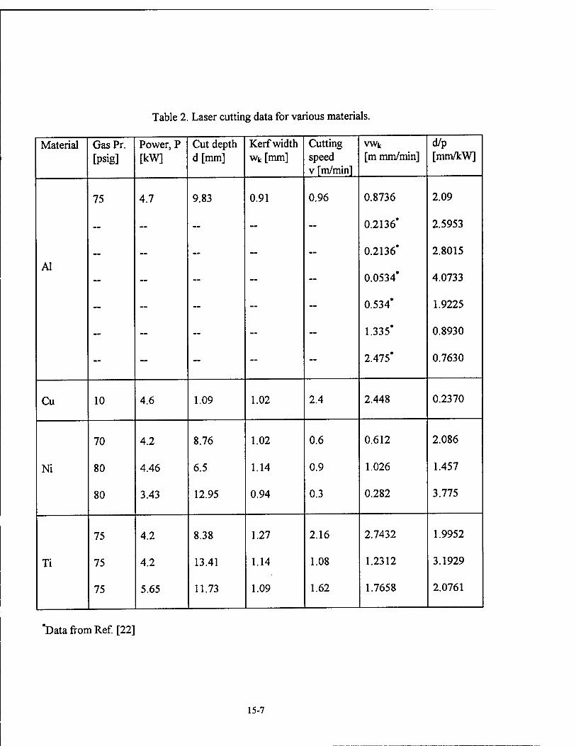
Table 2. Laser cutting data for various materials.
Material Gas Pr. [psig]
Power, P [kW]
Cut depth d [mm]
Kerf width wt [mm]
Cutting speed v [m/min]
VW|c
[m mm/min] d/p [mm/kW]
75 4.7 9.83 0.91 0.96 0.8736 2.09
— ~ — — — 0.2136* 2.5953
„ —m „ _ __ 0.2136* 2.8015
Al — — — — — 0.0534* 4.0733
— ~ — ~ — 0.534* 1.9225
— — — ~ — 1.335* 0.8930
— — — ~ — 2.475* 0.7630
Cu 10 4.6 1.09 1.02 2.4 2.448 0.2370
70 4.2 8.76 1.02 0.6 0.612 2.086
Ni 80 4.46 6.5 1.14 0.9 1.026 1.457
80 3.43 12.95 0.94 0.3 0.282 3.775
75 4.2 8.38 1.27 2.16 2.7432 1.9952
Ti 75 4.2 13.41 1.14 1.08 1.2312 3.1929
75 5.65 11.73 1.09 1.62 1.7658 2.0761
*Data from Ref. [22]
15-7
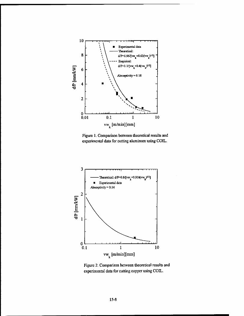
£ 6 -
vw [m/min] [mm]
Figure 1. Comparison between theoretical results and experimental data for cutting aluminum using COIL.
-i—i—i—i i i 11
Theoretical: dTMJ.S/fvw^O.QS^vw^W]
■ Experimental data Absorptivity =0.14
i
10
vw [m/min][mm]
Figure 2. Comparison between theoretical results and experimental data for cutting copper using COIL.
15-8
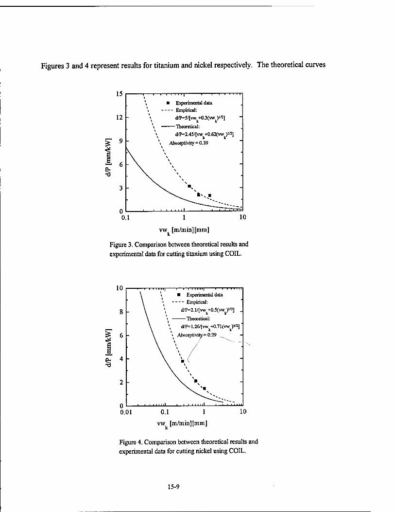
Figures 3 and 4 represent results for titanium and nickel respectively. The theoretical curves
15
12
*=■ 6
■ i i i i i i i i i i 1111 i \ ■ Experimental data
, Empirical:
\ d/P=5/[wv+0.3(vwk)i'3]
\ Theoretical: d/P=2.45/[vw +0.62(vwk)ifl]
Absorptivity = 0.39
vw [m/min][mm]
Figure 3. Comparison between theoretical results and experimental data for cutting titanium using COIL.
10
8 -
6 -
2 -
0.01
nrrrr —i—i i i i ii| i i—ill
Experimental data - Empirical:
d/P=2.1/[vw +0.5(vw )W]
Theoretical:
\ d/P=1.26/[vw +0.71(vwk)'«]
i Absorptivity*r(h29
• • "i i i i i i
10
vw [m/min][mm]
Figure 4. Comparison between theoretical results and experimental data for cutting nickel using COIL.
15-9

in these figures underestimate the cutting capability. Good agreement is achieved between the
theory and experiment by choosing Ao = 2.45 and A3 = 0.62 for titanium and Ao = 2.1 and A3 =
0.5 for nickel. Since the theory predicts the cutting data fairly well for aluminum and copper, it
suggests that the energy utilization mechanism during titanium and nickel cutting is different from
the cases of aluminum and copper.
Besides cutting experiments, the divergence angles and mode number for the COIL beam
are also evaluated in this study because the determine the optical quality of the laser. The
aluminum, copper and titanium cutting data in Table 2 except those taken from Ref. [22] were
obtained from a chemical oxygen-iodine laser (COIL) stable resonator with the z-pass
configuration in which the reflectors at the output coupler and diagonal pass were flat mirrors,
and the farthest reflector from the output coupler was a concave mirror. Circular laser beam was
produced by using a circular output aperture in the resonator. The divergence angles are
calculated at the output aperture based on the resonator and laser parameters given below. It
should be noted that the calculated divengence angles provide the theoretical minimum values that
are expected to be higher in practice due to the aberrations caused by the focusing lens.
Calculations of divergence angles for both circular and rectangular laser beams are presented
below for stable resonators.
4.1. Resonator parameters
Circular beam:
Radius of curvature of the output coupler, Ri = oo
Radius of curvature of the concave mirror, R2 = 2500 cm
Distance between the concave mirror and output coupler, L = 710 cm
Diameter of the output aperture, Da = 2.54 cm
Rectangular beam:
Radius of curvature of the output coupler, Ri = 00
Radius of curvature of the concave mirror, R2 = 2558 cm
Distance between the concave mirror and output coupler, L = 770 cm
15-10

Width of the output aperture in the x direction, Dx = 2.48 cm
Width of the output aperture in the y direction, Dy = 1.22 cm
4.2. Radius of the TEMnn mode at the output aperture. Wo for stable resonators
A/2
,23
0 7t glg20-8iS2)
[(gl+g2-2glg2)2J , gi = 1 - L/Ri, and g2 = 1 - L/R2
4.3. Beam parameters for the higher order Gaussian COIL beam of wavelength. \ = 1.315 urn
Circular beam of mode TEMp/:
wo = 0.217228 cm
Mode number, M = (2p+/+l)1/2 = Da/(2w0) = 5.846392
Divergence of the TEMoo mode, 0 = 2A/(7tw0) = 0.38538 mrad
Divergence of the TEMp/ mode, 9P/ = M0 = 2.253 mrad
Rectangular beam of mode TEMmn:
wo = 0.2216167 cm
Half-length of the waist in the x direction, w0x = 0.2216167 cm
Half-width of the waist in the y direction, w0y = 0.2216167 cm
Mode number in the x direction, Mx = (2m+l)1/2 = Dx/(2w0x) = 5.595
Mode number in the y direction, My = (2n+l)1/2 = Dy/(2w0y) = 2.753
Divergence of the TEMoo mode in the x direction, 0X = X/(7iw0x) = 0.18887 mrad
Divergence of the TEMoo mode in the y direction, 0y = X/(7CW0y) = 0.18887 mrad
Divergence of the TEMmn mode in the x direction, On™ = MX0X = 1.0567 mrad
Divergence of the TEMmn mode in the y direction, ©„„.y = My0y = 0.52 mrad
5. Conclusions
Experiments have been conducted to cut different types of materials, and the data are
compared with the results obtained from a scaling law. The scaling law for cut depth per unit
power, d/P, agrees well with the experimental data for aluminum and copper, and deviates
appreciably from the titanium and nickel cutting data. This suggests that the mechanism of the
15-11

laser and thermal energy utilization during aluminum and copper cutting is different from the cases
of titanium and nickel cutting. The COIL beams used in the cutting experiments had very few
higher order modes.
Nomenclature
A Absorptivity of the substrate at the laser-material interaction zone
a Thermal diffusivity of the substrate
ß "Boiling coefficient", the fraction of the kerf width above the boiling temperature
Cp Specific heat of the substrate at constant pressure
d Kerf depth
k Thermal conductivity
/ Length of the rectangular COIL beam spot
Lb Latent heat of boiling
Lm Latent heat of melting
P Laser power of the incident beam at the surface of the workpiece
Tm Melting temperature of the substrate
To Initial temperature of the substrate
v Velocity of the scanning laser beam
Wk Kerf width
References
1. A. Kar, J. E. Scott and W. P. Latham, "Theoretical and Experimental Studies of Thick-
Section Cutting with a Chemical Oxygen-Iodine Laser (COIL)," J. Laser Applications, Vol. 8,
1996, pp. 125-133.
2. T. Atsuta, K. Yasuda, T. Matsumoto, T. Sakurai and H. Okado, "COIL and the Material
Processing," in Conference on Lasers and Electro-Optics (CLEO)'94, Vol. 8, 1994, OSA
Technical Digest Series (Optical Society of America, Washington D. C), P. 351, 1994.
3. A. V. Tikhomirov, "State of Laser Cutting Technology and Prospects for its Development,"
Bull. Academy of Sciences of the USSR, Vol. 47. 1983, pp. 23-28.
15-12
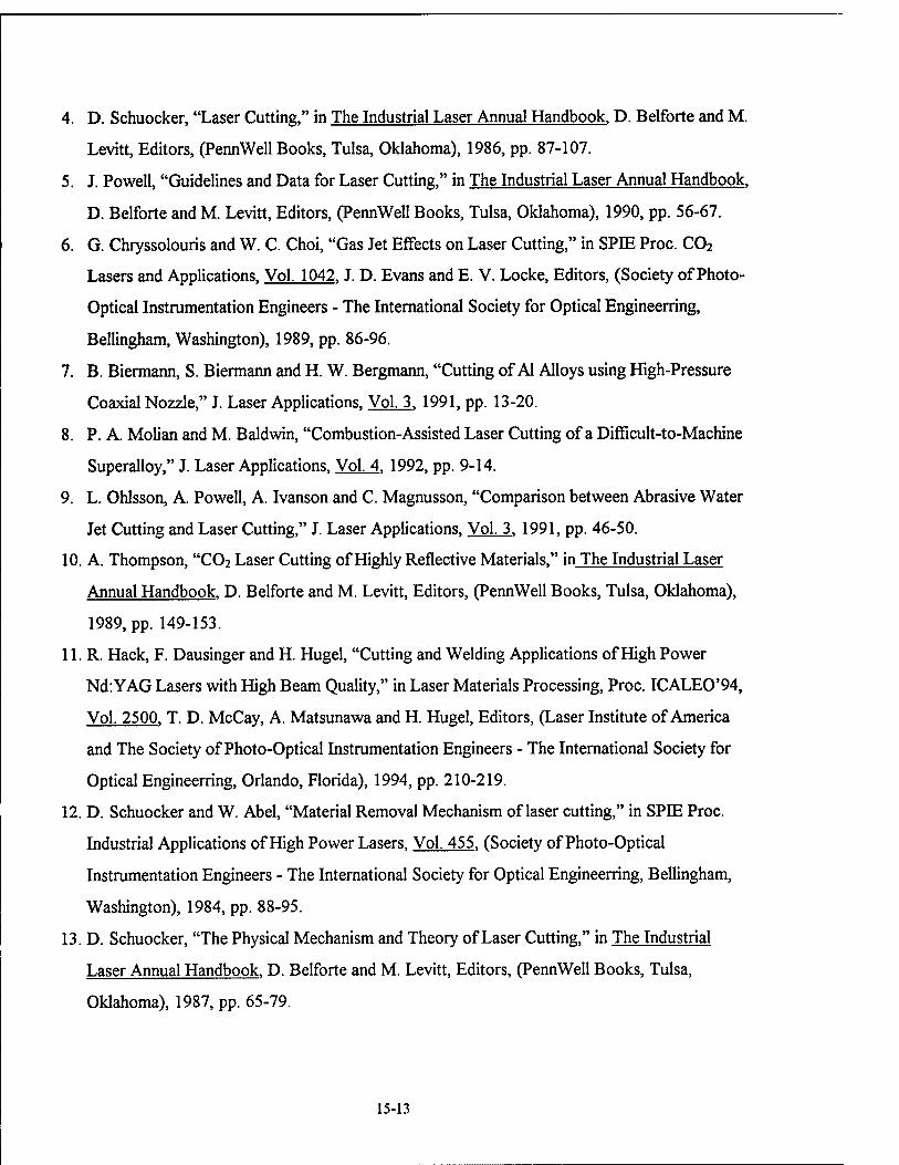
4. D. Schuocker, "Laser Cutting," in The Industrial Laser Annual Handbook, D. Belforte and M.
Levitt, Editors, (PennWell Books, Tulsa, Oklahoma), 1986, pp. 87-107.
5. J. Powell, "Guidelines and Data for Laser Cutting," in The Industrial Laser Annual Handbook.
D. Belforte and M. Levitt, Editors, (PennWell Books, Tulsa, Oklahoma), 1990, pp. 56-67.
6. G. Chryssolouris and W. C. Choi, "Gas Jet Effects on Laser Cutting," in SPIE Proc. C02
Lasers and Applications, Vol. 1042, J. D. Evans and E. V. Locke, Editors, (Society of Photo-
Optical Instrumentation Engineers - The International Society for Optical Engineerring,
Bellingham, Washington), 1989, pp. 86-96.
7. B. Biermann, S. Biermann and H. W. Bergmann, "Cutting of Al Alloys using High-Pressure
Coaxial Nozzle," J. Laser Applications, Vol. 3, 1991, pp. 13-20.
8. P. A. Molian and M. Baldwin, "Combustion-Assisted Laser Cutting of a Difflcult-to-Machine
Superalloy," J. Laser Applications, Vol. 4. 1992, pp. 9-14.
9. L. Ohlsson, A. Powell, A. Ivanson and C. Magnusson, "Comparison between Abrasive Water
Jet Cutting and Laser Cutting," J. Laser Applications, Vol. 3. 1991, pp. 46-50.
10. A. Thompson, "C02 Laser Cutting of Highly Reflective Materials," in The Industrial Laser
Annual Handbook, D. Belforte and M. Levitt, Editors, (PennWell Books, Tulsa, Oklahoma),
1989, pp. 149-153.
U.R. Hack, F. Dausinger and H. Hugel, "Cutting and Welding Applications of High Power
Nd: YAG Lasers with High Beam Quality," in Laser Materials Processing, Proc. ICALEO'94,
Vol. 2500, T. D. McCay, A. Matsunawa and H. Hugel, Editors, (Laser Institute of America
and The Society of Photo-Optical Instrumentation Engineers - The International Society for
Optical Engineerring, Orlando, Florida), 1994, pp. 210-219.
12. D. Schuocker and W. Abel, "Material Removal Mechanism of laser cutting," in SPIE Proc.
Industrial Applications of High Power Lasers, Vol. 455, (Society of Photo-Optical
Instrumentation Engineers - The International Society for Optical Engineerring, Bellingham,
Washington), 1984, pp. 88-95.
13. D. Schuocker, "The Physical Mechanism and Theory of Laser Cutting," in The Industrial
Laser Annual Handbook, D. Belforte and M. Levitt, Editors, (PennWell Books, Tulsa,
Oklahoma), 1987, pp. 65-79.
15-13
14. L. Li and J. Mazumder, "A Study of the Mechanism of Laser Cutting of Wood," Forest
Products Journal, Vol. 41. 1991, pp. 53-59.
15. M. F. Modest and H. Abakians, "Evaporative Cutting of a Semi-Infinite Body with a Moving
CW Laser," J. Heat Transfer, Vol. 108. 1986, pp. 602-607.
16. S. Y. Bang and M. F. Modest "Multiple Reflection Effects on Evaporative Cutting with a
Moving CW Laser," J. Heat Transfer, Vol. 113. 1991, pp. 663-669.
17. S. Roy and M. F. Modest "Evaporative Cutting with a Moving CW Laser - Part I: Effects of
Three-Dimensional Conduction and Variable Properties," Int. J. Heat Mass Transfer, Vol. 36.
1993, pp. 3515-3528.
18.1. Belie and J. Stanic, "A Method to Determine the Parameters of Laser Iron and Steel
Cutting," Optics and Laser Technology, Vol. 19. 1987, pp. 309-311.
19.1. Belie, "A Method to Determine the Parameters of Laser Cutting," Optics and Laser
Technology, Vol. 21. 1989, pp. 277-278.
20. A. Kar, J. E. Scott and W. P. Latham, Effects of mode structure on three-dimensional laser
heating due to single or multiple rectangular laser beams, J. Appl. Phys., Vol. 80. 1996, pp.
667-674.
21. J. Xie, A. Kar, J. A. Rothenflue and W. P. Latham, "Temperature-Dependent Absorptivity
and Cutting Capability of C02, Nd:YAG and Chemical Oxygen-Iodine Lasers," J. Laser
Applications, Vol. 9. 1997, pp. 77-85.
22. D. L. Carroll and J. A. Rothenflue, "Experimental Study of Cutting Thick Aluminum and
Steel with a Chemical Oxygen-Iodine Laser using N2 or 02 gas assist," In: Proc. XI Inter.
Symp. Gas Flow and Chemical lasers and High Power Laser (GCL/HPL'96), Edinburgh,
Scotland, UK.
23. A. E. Siegman, Lasers, University Science Books, New York, 1986, pp. 663-685.
15-14
QUANITUM CHEMICAL CHARACTERIZATION OF THE ELECTRONIC STRUCTURE AND REACTIONS OF SILICON DANGLING BONDS IN Si/ Si02
REACTIONS OF H2 AND H AT THE SILICON (111) INTERFACE
Bernard Kirtman Associate Professor
Department of Chemistry
University of California Santa Barbara, California 93106
Final Report for: Summer Research Program
Phillips Laboratory
Sponsored by: Air Force Office of Scientific Research
Boiling Air Force Base, Washington, DC
And
Phillips Laboratory
September 1997
16-1
QUANTUM CHEMICAL CHARACTERIZATION OF THE ELECTRONIC STRUCTURE AND REACTIONS OF SILICON DANGLING BONDS IN Si/SiOz.
REACTIONS OF H2 AND H AT THE SILICON (111) INTERFACE.
Bernard Kirtman Professor
Department of Chemistry University of California, Santa Barbara
Abstract
The finite cluster method is employed to calculate activation energies for the
passivation/depassivation reactions of hydrogen with the dangling bond center at
the (111) Si/SiOz interface. Initial results including only nearest neighbors do not
reproduce the experimental values. It is shown that an accurate and reliable
quantum chemical treatment is feasible for a large cluster model using a general
"model within a model" approach. Possible further simplifications are discussed
along with future applications and developments.
16-2

QUANTUM CHEMICAL CHARACTERIZATION OF THE ELECTRONIC STRUCTURE AND REACTIONS OF SILICON DANGLING BONDS IN Si/Si02.
REACTIONS OF H2 AND H AT THE SILICON (111) H^TERFACE.
Bernard Kirtman
Introduction
The creation of a silicon surface will leave unpaired electrons in dangling bonds
located at the silicon atoms where Si-Si bonds have been broken. In the production
of metal/oxide/silicon (MOS) devices most of these sites are passivated by the
thermal oxidation which is used to form the amorphous SiOz (a-Si02) layer.
However, the defect sites that remain at the Si/SiOz interface (known as Pb centers)
are electrically active and sufficient in number to seriously impede device performance. It has been found {1} that annealing at ~ 400° C in a hydrogen ambient leads to a dramatic decrease in their density, which tends to resolve this difficulty. On the other hand, the devices can be damaged by hot electrons or radiation which
causes depassivation due to (re-)generation of Pb centers. In either case the damage is
enhanced by the presence of hydrogen {2-5}. Thus, characterization of reactions
involving the interfacial Pb defects with hydrogenic species is crucial to understanding the passivation/depassivation of MOS devices.
The properties of a particular Pb center will depend upon its nearest neighbors
and, to a greater or lesser extent, on the non-local environment as well. From an experimental point of view the most potent tool for characterizing the local geometry has been ESR spectroscopy {6}. On the basis of ESR a single dangling bond
center, known simply as Pb , has been identified at the (111) interface and two
centers, known as Pb0 and PM , at the (100) interface. The g-tensors observed for Pb and Pb0 are almost identical. Both exhibit axial (or near axial) symmetry about the (111) direction with component values that are typical of silicon dangling bond centers
having three silicon atoms as nearest neighbors. The 29Si hyperfine satellite data for these two centers yields A-tensor parameters that are consistent with the above analysis and yield an estimated p-character substantially greater than sp3 for the dangling bond orbital. It is interesting that the Pbl g-tensor shows a deviation from axial symmetry in the (111) direction, although the component values are not very dissimilar from Pb0 and Pbv The one hyperfine measurement carried out for Pbl at a
16-3
single orientation shows that the separation of the satellite lines is comparable to that of Pb0.
The primary ESR signal can also be used to monitor the density of paramagnetic centers during the course of a reaction. In particular, this technique has been used to obtain rate constants for H2 passivation of Pb centers and for dissociation of hydrogen atoms from the (diamagnetic) passivated HPb defect. For
the (111) interface Brower {7} found that the rate of passivation by H2 is proportional
to the density of Pb centers at the interface and to the H2 concentration. From this
one may infer the reaction:
Pfc+H2 -> HPb + H (1)
The observed rate constant, measured as a function of temperature in the range
230°-260° C, is accurately described by the Arrhenius equation with an activation energy Ea
f= 1.66 ± .06 eV. Subsequent vacuum thermal annealing of the passivated HPb centers in the temperature range 500°-600° C leads to recovery of paramagnetic Pb. Since the dissociation rate is proportional to the HPfc density, and there is a large deuterium isotope effect, it was concluded {8,9} that the pertinent reaction is:
HPb—>Pb + H; Ed = 2.56eV (2)
Again, the rate constant data is well fit {8,9} by the Arrhenius expression giving an
activation energy for dissociation of Ed = 2.56 ± 0.06 eV. In addition to the passivation reaction of Eq.(l) it is useful to consider the
reverse abstraction reaction. Thus, if TS refers to the common transition state, then -
Pb+ H2 —> TS; Eaf=1.66eV (3a)
and HP, + H — > TS Ea
r. (3b)
Evidently, the combination Eq.(3a) - Eq.(3b) + Eq.(2) corresponds to the overall reaction -
H2 — > 2H.
This means that Eaf - Ea
r + Ed = 4.22 eV - Ear should equal {10} the dissociation energy
of H2 in Si02. It has been argued {8,9} that the latter cannot be very different from the
dissociation energy of H2 in vacuo, which is 4.52 eV. That being the case, Ear should
16-4
be close to 0.0 eV since any greater value will increase the discrepancy beyond 0.30
eV. Passivation kinetics corresponding to Eq.(3a) have been investigated {11} for
the Pb0 and Pbl centers at the (100) interface over the temperature range 213°-234° C.
Although the results were similar to those obtained at the (111) surface, it was found
that the data could not be fit by a single-valued Eaf. Thus, the activation energies
were determined as a mean value plus a Gaussian spread. For the Pb0 and Pbl centers
Eaf = 1.51 ± 0.30 eV and 1.57 ± 0.30 eV respectively. As far as the activation energies
are concerned Pbl is somewhat closer to Pb than is Pb0. Indeed, on the basis of several
different passivation experiments, Stathis and co-workers {12-14} have argued that
Pb0 is certainly different from Pb and that the latter behaves more like PM. Very
recently, Vanheusden, et ah {15} have made analogous observations in the course of examining Si/Si02/Si structures. In this regard, then, there is an inconsistency between ESR and hydrogen passivation studies that remains to be resolved.
Quantum chemical calculations may be able to play a significant role in
characterizing the several Pb centers. In principle, such calculations can be used to test atomic scale models based on the interpretation of experimental data. Different models can be compared and new experiments suggested to verify predicted structures. In order to succeed, however, it must be demonstrated that the
computational methods employed are of sufficient accuracy and reliability. Thus, we
focused our attention initially on determining activation energies for hydrogen
passivation/depassivation at the (111) Pb center. This is the center that is best characterized experimentally and stationary points on the reactive potential energy
surface (equilibrium geometries and energies; TS geometries and energies) are the
most straightforward properties to obtain. Once a satisfactory approach has been developed, then the stage will be set for
branching out in several directions. Thus, we will be able to investigate the technologically dominant Pb0 and Pbl centers at the (100) interface. Also of interest are
the radiation-induced (as well as intrinsic) E' silicon dangling bond centers in the a-
Si02 layer that are thought {16} to play a key role in the transport of hydrogenic
species to the Si/Si02 interface. This is not to mention the occurrence of oxygen paramagnetic centers which, so far, have been of lesser concern.
Other key properties apart from activation energies will also become accessible. The electronic g-tensors and hyperfine coupling tensors fall into this
16-5

category. Measurements have also been made {17,18} which yield the population of Pb electronic energy levels within the silicon bandgap as a function of the position of the Fermi level. Computation of this property can provide yet another important handle on the microscopic characterization of the Pb center.
The use of quantum chemical computations as an interpretive tool of its own is worthy of mention here. From such calculations one can distinguish between
local contributions to physical properties and medium-long range effects.
Furthermore, it is possible to analyze results in terms of classical electrostatics,
exchange effects, electron correlation, ... and to investigate the role of through-bond
vs. through-space interactions, orbital hybridization, etc.
In the next section we discuss briefly three main approaches that may be
utilized to carry out quantum chemical modeling of large aperiodic systems. Of
these the finite cluster treatment has been chosen for our initial studies. In order to combine practicality with accuracy and reliability a variety of what may be called "model within a model" techniques are employed. Similar techniques have been used in the past to improve the accuracy for a given finite cluster and, recently, a general approach to extending the size of the cluster has been presented by Morokuma and co-workers {19-23}. Both modalities are employed here with systematic testing in so far as possible. In addition, it is shown that the treatment of Morokuma, et al. may be extended to give the local geometry at stationary points
directly rather than through an indirect energy optimization. The "model within a model" method for large clusters requires a high level
treatment of a small cluster followed by correction for the difference between the large cluster and the small one obtained at a lower level. The small cluster is defined in the third section where it is also demonstrated that calculations can be done at a sufficient accuracy for our purposes. Then we construct the large cluster, test various lower levels of treatment and consider further reductions of level. Finally, the major conclusions of this work are presented along with a discussion of proposed
future developments.
Methods There are three major approaches to the quantum chemical treatment of large aperiodic systems. The one that we shall utilize here is the most straightforward, namely the finite cluster method. It assumes that the property in question is
16-6
sufficiently local so that it can be well-represented by means of a relatively small finite cluster molecular model. In applying this method the dependence of the
property on cluster size should be carefully monitored for convergence. A variety of techniques are available for embedding a small cluster within a
larger system. All of these, either implicitly or explicitly, make some approximation
regarding the interaction terms. This leads to an "effective" Hamiltonian, or an "effective" projected Hamiltonian, which is used to represent the embedded cluster.
Although we do not employ an embedding technique in this investigation it is a
consideration for the future as noted in the final section.
The third general approach is the supercell method. It is the theoretical
analogue of biomolecular crystallography. That is to say, one defines a unit cell
containing a finite cluster model and reproduces that cell so as to form an infinite
periodic array. This makes it possible for band structure computational techniques to be applied. The supercell method does not appear to be advantageous for the current
investigation and will, therefore, not be considered further. If it were possible to determine accurate and reliable electronic structures
from semiempirical calculations, then it would be feasible to treat large finite
clusters directly. In order to test that proposition we carried out MNDO calculations on the first nearest neighbors (NN=1) cluster model. As shown in Fig. 1(b) the nearest neighbor silicons are terminated by hydrogen atoms. In the TS of Eqs.(3a) and (3b) the silicon Pb center and the original H2 molecule are linearly aligned as expected. The Pb-H distance, Rx, and the H-H distance, R2, are reported in Table I where it is clear that very different values are obtained by a high level ab initio
treatment (to be discussed later). Likewise large discrepancies (0.78,1.00 eV) can be seen for Ea
f and Ed. This confirms the lore that semiempirical methods are
inadequate for transition states. The same is true for molecular force fields, i.e.
molecular mechanics. We conclude that ab initio methods are required to give even reasonable TS
results for small model clusters. In fact, we will see that only a high level ab initio
treatment will provide Eaf, Ea
r and Ed to within the desired accuracy of 0.05 eV. This does not mean that lower level ab initio calculations, or even a semiempirical treatment, will be unsuitable for accomplishing the transition from small to large clusters. In fact, as mentioned in the Introduction, Morokuma and co-workers {19- 23} have presented a general framework for achieving high accuracy using lower
16-7
level methods. The general (approximate) relation that they exploit may be written as-
(large; high level) = (small; high level) + [(large; lower level) - (small; lower level)] (4)
It is presumed that the correction term in square brackets may be evaluated with
sufficient accuracy at a lower level of treatment. Of course, the definition of "high
level" and "lower level" must be specified and, for that matter, the same is true of
"small" and "large". In arriving at the definitions tests should be carried out to
verify that a justifiable claim of accuracy can be made. Eq.(4) is a one-step procedure.
Of course, it is also possible to make the transition from the small to large cluster
through any number of intermediate steps as Morokuma, et al. have noted. Morokuma's prescription has been used to determine energies and, thereby, stationary point geometries. We will see that it can also be employed directly to obtain values for local internal coordinates at the stationary points.
In ab initio calculations, the level is specified by the electronic structure method and the basis set indicated by (method/basis). For a given cluster a desired (accurate/large) result may be estimated from -
(accurate/large) = (less accurate/smaller) + [(accurate/smaller) - (less accurate/smaller)]
+ [(less accurate/large) - (less accurate/smaller)] (5) This relation presumes that the method and basis set corrections are additive. The validity of Eq.(5), like that of Eq.(4), must be established for each individual case. In this study we will see that it can be used to obtain a high level small cluster result to be used for the first term on the rhs of Eq.(4).
Small Model Clusters The first small cluster that we examined was the model without any nearest neighbors, i.e. NN=0 in Fig.l(a). It may be noted that the value of Ea
f for the (111) Pb
center is not very different from that of the (100) Pw and Pbl centers. Indeed all three values lie within the range 1.51-1.66 eV. Thus, an NN=0 cluster model is not
entirely absurd.
16-8
A UMP2/6-31G** calculation is generally sufficient for determining a good
geometry. So this is where we began. The key TS structural parameters, i.e. Rt and
R2, obtained at this level are reported in Table 11(A). By comparison with UMP2/6- 31 IG** we see that the basis set is adequate. On the other hand, upon going from
UMP2 to CCSD(T) Ra and R2 change by 0.02 Ä and 0.06 Ä respectively. We conclude
that CCSD(T) is required for an accurate TS geometry. If CCSD(T) is taken as the
standard, then the UHF bond lengths show substantially larger errors than the MP2
values. The commonly used B3LYP version of density functional theory will often
give equilibrium geometries that are closely comparable to MP2. Recently, Truong
{24} has pointed out that the same is not true for transition states. He has found,
however, that Becke's {25} Half and Half (BHH) treatment of electron exchange
along with the Lee, Yang and Parr {26} correlation potential (LYP) will give
satisfactory results. We have confirmed Truong's observations for the NN=0 cluster
model. The last column of Table 11(A) shows that, compared to CCSD(T), the error in
both Rj and R2 has about the same magnitude as for MP2, but is opposite in sign. What surprised us was the fact that the BHHLYP geometry optimization took much
longer than MP2 to execute using GAUSSIAN94. Although CCSD(T) is required for an accurate TS geometry, such a high
quality geometry is not necessary in order to obtain accurate activation energies. This is demonstrated in Table 11(B) where we show the results of CCSD(T) energy
calculations carried out at the MP2 and CCSD(T) geometries. In all circumstances a 6-
31G** basis set was employed. As we've already seen that this basis yields satisfactory geometries (its suitability for the calculation of activation energies will be discussed shortly). Evidently, the differences in Ea
f, Ear and Ed for the two geometries are on the
order of 0.01 eV, which means that the MP2/6-31G** geometry should be sufficient
for our purposes. The next step was to determine the effect of increasing the level of treatment
for the energies with the geometry calculations done always at the MP2/6-31G**
level. In Table 11(C) the first two rows yield a comparison of MP2 values for Eaf, Ea
r
and Ed obtained with either the 6-311G** or the 6-31G** basis set. The discrepancy between the two rows ranges from 0.043 eV for Ed to 0.111 eV for Ea
f. We conclude that the difference between a valence double zeta and a valence triple zeta basis is small but significant. Adding additional diffuse functions (for both hydrogen and
16-9
silicon), as in the last row of the table, leads to negligible changes ( <~ 0.005 eV ). By comparing the first and third rows we obtain the effect of using the CCSD(T) method rather than MP2 with the same 6-31G** basis in either case. It turns out that the effect varies from 0.006 eV for Ea
f to 0.107 eV for Ear to 0.103 for Ed. In this case our
conclusion is that the effect is, again, small but significant. On the basis of the calculations reported in Table II we judge that the desired
high level treatment for the small model cluster in Eq.(4) is CCSD(T)/6-
311G**//MP2/6-31G**. Is it satisfactory to reach this level using Eq.(5) with MP2/6-
31G*V/MP2/6-31G** as the starting point? A test of that notion for the NN=0
cluster is provided in Table III. The first row of the table gives the "exact" result and
the last row the predicted value. Rows 2 and 3 are the corrections due to the basis set and the method respectively. The total correction varies in magnitude from 0.117 to 0.160 eV while the error in the predicted value is less than 0.026 eV for each activation energy. It appears that the goal of 0.10 eV accuracy in the final result can be met by the approximate additive approach of Eq.(5).
It is straighforward to extend the approximate calculations of Table HI to the NN=1 cluster. A summary of the values obtained for NN=0, NN=1 and experiment is provided in Table IV. Note that including first nearest neighbors leads to substantial changes in the (non-observable) TS geometry. It is also true that, in each
case, the presence of the first neighbors leads to significantly improved agreement with experiment. However, the remaining discrepancy is still large. It is certainly
larger than one might expect {27} from corrections to the barrier height due to zero- point vibrations, tunneling, etc. Thus, one must conclude that it is critical to take account of more distant neighbors and/or non-bonding interactions with atoms in the a-Si02 layer. Alternatively, one may have to consider the possibility that the experimental interpretation is not completely correct.
Large Cluster Model The addition of second nearest neighbors to form the NN=2 cluster model includes
more silicons but introduces no new qualitative features. With third nearest neighbors (see Fig.2) oxygen atoms appear for the first time and closed silicon rings as well. Since the effect of these features would need to be investigated in any event it was decided to skip the NN=2 case and proceed immediately to the simplest model which has oxygen and closed silicon rings. Thus, we constructed a Si1906H27
16-10
cluster containing: (1) all second nearest neighbors, plus (2) all third nearest
neighbor oxygen atoms, plus (3) all third nearest neighbor silicon atoms that give
rise to ring closure. The resulting cluster model is presented in Fig.2. (not shown are the terminating hydrogen atoms). A similar model has been investigated by
Edwards {28,29} who included all third nearest neighbors and carried out an MNDO
electronic structure calculation. For the large Si1906H27 cluster we employ the general approach of Eq.(4). The
low level treatment considered initially was UHF/6-31G**. As a test we carried out
calculations in which the NN=0 model was taken to be the small cluster and the NN=1 model the large cluster. An argument can be made that this is a worst case
scenario. The results reported in Table IV were obtained using a 6-31G** basis throughout; thus only the method is listed. It is readily seen from the table that the
UHF//UHF energy corrections reproduce the CCSD(T)//MP2 values to within 0.015
eV for Eaf, Ea
r and Ed. The numbers in parentheses are the best high level estimates found by applying Eq. (5) to determine CCSD(T)/6-311G**//MP2/6-31G** values as described earlier. In comparison with the latter our conclusion given above (i.e.
agreement of UHF/ /UHF to within 0.015 eV) remains unchanged. Since geometry optimization is the most time-consuming step we have
undertaken some calculations to see if the UHF/3-21G geometry would be acceptable instead of UHF/6-31G**. Table V(A) shows that there is remarkably close agreement
(0.005 eV) between UHF activation energies obtained with the two different
geometries. Indeed, this close agreement prompted us to look at the possibility of
utilizing Eq.(4) directly to predict the geometry of large clusters. We focused specifically on the TS parameters Rt and R2 since they are, by far, the most sensitive to changes in the description of the electronic structure. The values reported in Table V(B) show that the difference in these bond lengths due to transition from the
NN=0 to the NN=1 cluster varies little, i.e. < 0.006 Ä, from a UHF/3-21G to a UHF/6-31G** calculation. The variation from UHF/6-31G** to MP2/6-31G** is a bit
larger, but still less than 0.036 Ä (out of 0.111 Ä for the difference between NN=0 and
NN=1) in the worst case. Accurate calculations for the large cluster are feasible at the UHF/6-31G**//
UHF/3-21G level of approximation. However, such a treatment requires extensive computational resources. Further simplifications will, therefore, be explored before proceeding along this path. As far as geometry optimization is concerned, it should
16-11
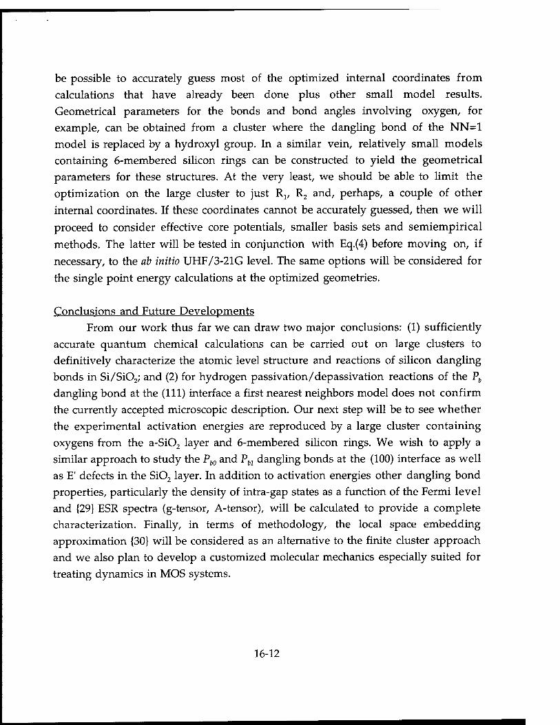
be possible to accurately guess most of the optimized internal coordinates from calculations that have already been done plus other small model results. Geometrical parameters for the bonds and bond angles involving oxygen, for example, can be obtained from a cluster where the dangling bond of the NN=1 model is replaced by a hydroxyl group. In a similar vein, relatively small models containing 6-membered silicon rings can be constructed to yield the geometrical parameters for these structures. At the very least, we should be able to limit the
optimization on the large cluster to just Ra, R2 and, perhaps, a couple of other
internal coordinates. If these coordinates cannot be accurately guessed, then we will
proceed to consider effective core potentials, smaller basis sets and semiempirical
methods. The latter will be tested in conjunction with Eq.(4) before moving on, if
necessary, to the ab initio UHF/3-21G level. The same options will be considered for
the single point energy calculations at the optimized geometries.
Conclusions and Future Developments From our work thus far we can draw two major conclusions: (1) sufficiently
accurate quantum chemical calculations can be carried out on large clusters to definitively characterize the atomic level structure and reactions of silicon dangling bonds in Si/Si02; and (2) for hydrogen passivation/depassivation reactions of the Pb
dangling bond at the (111) interface a first nearest neighbors model does not confirm the currently accepted microscopic description. Our next step will be to see whether the experimental activation energies are reproduced by a large cluster containing oxygens from the a-SiOz layer and 6-membered silicon rings. We wish to apply a similar approach to study the Pb0 and Pbl dangling bonds at the (100) interface as well as E' defects in the SiOz layer. In addition to activation energies other dangling bond properties, particularly the density of intra-gap states as a function of the Fermi level and {29} ESR spectra (g-tensor, A-tensor), will be calculated to provide a complete characterization. Finally, in terms of methodology, the local space embedding approximation {30} will be considered as an alternative to the finite cluster approach and we also plan to develop a customized molecular mechanics especially suited for
treating dynamics in MOS systems.
16-12
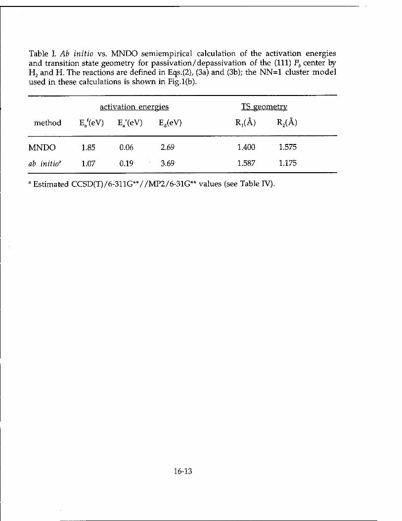
Table I. Ab initio vs. MNDO semiempirical calculation of the activation energies and transition state geometry for passivation/depassivation of the (111) Pb center by H2 and H. The reactions are defined in Eqs.(2), (3a) and (3b); the NN=1 cluster model used in these calculations is shown in Fig.1(b).
activation energies TS geometry
method Eaf(eV) E/(eV) Ed(eV) RX(Ä) R2(Ä)
MNDO 1.85 0.06 2.69 1.400 1.575
ab initio3 1.07 0.19 3.69 1.587 1.175
a Estimated CCSD(T)/6-311G*V/MP2/6-31G** values (see Table IV).
16-13
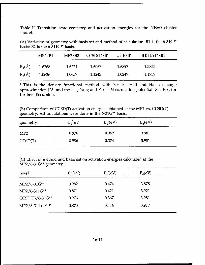
Table II. Transition state geometry and activation energies for the NN=0 cluster model.
(A) Variation of geometry with basis set and method of calculation. Bl is the 6-31G** basis; B2 is the 6-31 IG** basis.
MP2/B1 MP2/B2 CCSD(T)/B1 UHF/B1 BHHLYP7B1
R^A) 1.6268 1.6221 1.6067 1.6897 1.5835
R2(A) 1.0636 1.0657 1.1243 1.0249 1.1759
a This is the density functional method with Becke's Half and Half exchange approximation {25} and the Lee, Yang and Parr {26} correlation potential. See text for further discussion.
(B) Comparison of CCSD(T) activation energies obtained at the MP2 vs. CCSD(T) geometry. All calculations were done in the 6-31G** basis.
geometry E>V) E/(eV) Ed(eV)
MP2 0.976 0.367 3.981
CCSD(T) 0.986 0.374 3.981
(C) Effect of method and basis set on activation energies calculated at the MP2/6-31G** geometry.
level Eaf(eV) E/(eV) Ed(eV)
MP2/6-31G** 0.982 0.474 3.878
MP2/6-311G** 0.871 0.421 3.921
CCSD(T)/6-31G** 0.976 0.367 3.981
MP2/6-311++G** 0.870 0.416 3.917
16-14
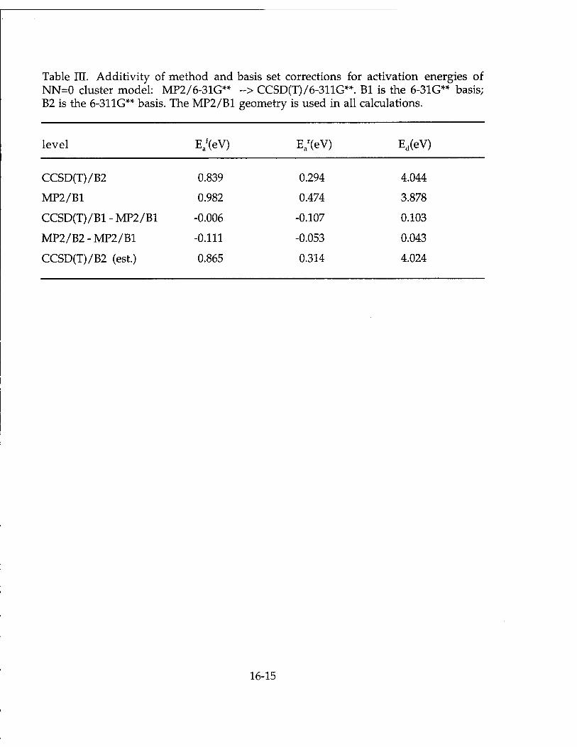
Table III. Additivity of method and basis set corrections for activation energies of NN=0 cluster model: MP2/6-31G** -> CCSD(T)/6-311G**. Bl is the 6-31G** basis; B2 is the 6-311G** basis. The MP2/B1 geometry is used in all calculations.
level E/(eV) E/(eV) Ed(eV)
CCSD(T)/B2 0.839 0.294 4.044
MP2/B1 0.982 0.474 3.878
CCSD(T)/B1-MP2/B1 -0.006 -0.107 0.103
MP2/B2 - MP2/B1 -0.111 -0.053 0.043
CCSD(T)/B2 (est.) 0.865 0.314 4.024
16-15
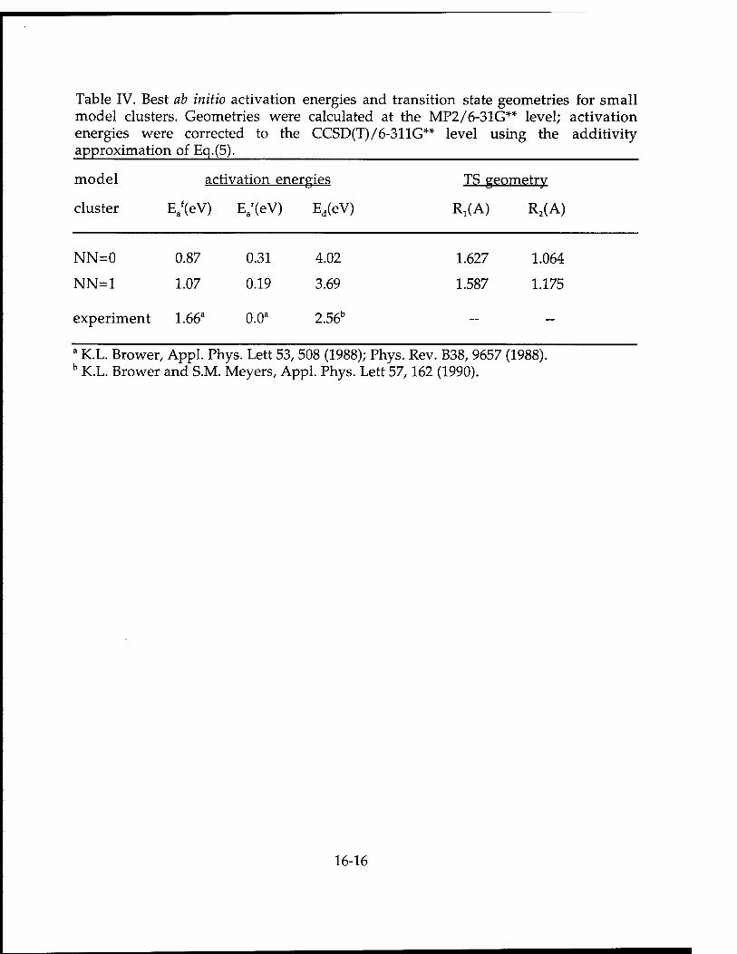
Table IV. Best ab initio activation energies and transition state geometries for small model clusters. Geometries were calculated at the MP2/6-31G** level; activation energies were corrected to the CCSD(T)/6-311G** level using the additivity approximation of Eq.(5).
model activation energies TS geometrv
cluster Eaf(eV) E/(eV) Ed(eV) Ri(A) R2(A)
NN=0 0.87 0.31 4.02 1.627 1.064
NN=1 1.07 0.19 3.69 1.587 1.175
experiment 1.66a 0.0a 2.56b —
a K.L. Brower, Appl. Phys. Lett 53,508 (1988); Phys. Rev. B38, 9657 (1988). b K.L. Brower and S.M. Meyers, Appl. Phys. Lett 57,162 (1990).
16-16
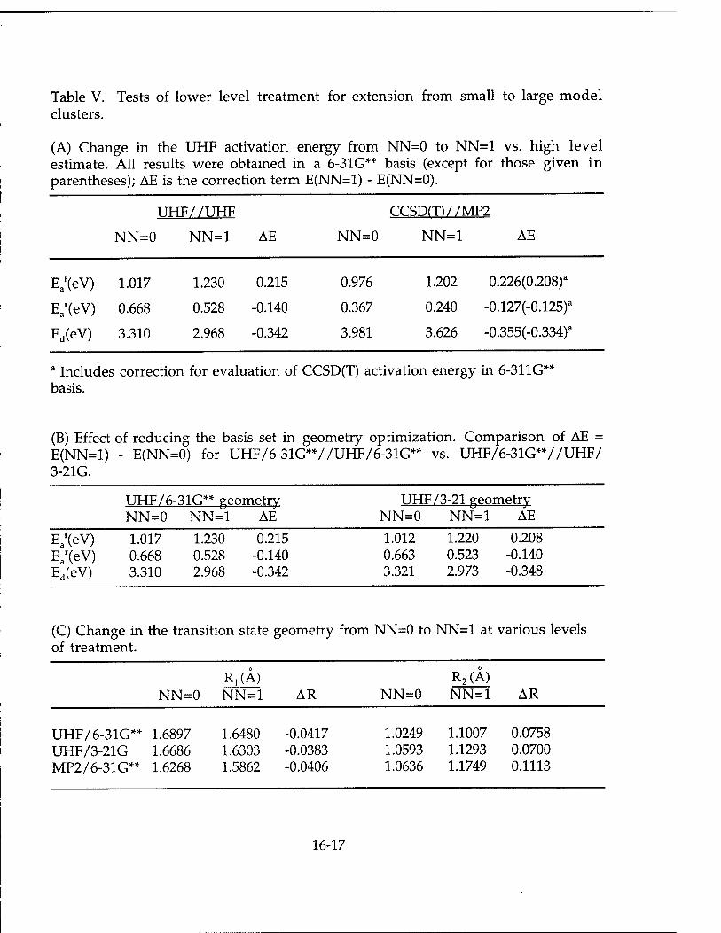
Table V. Tests of lower level treatment for extension from small to large model clusters.
(A) Change in the UHF activation energy from NN=0 to NN=1 vs. high level estimate. All results were obtained in a 6-31G** basis (except for those given in parentheses); AE is the correction term E(NN=1) - E(NN=0).
UHF/ /UHF CCSPm//MF2
NN=0 NN=1 AE NN=0 NN=1 AE
E>V) 1.017 1.230 0.215 0.976 1.202 0.226(0.208)a
E/(eV) 0.668 0.528 -0.140 0.367 0.240 -0.127(-0.125)a
Ed(eV) 3.310 2.968 -0.342 3.981 3.626 -0.355(-0.334)a
a Includes correction for evaluation of CCSD(T) activation energy in 6-31 IG** basis.
(B) Effect of reducing the basis set in geometry optimization. Comparison of AE = E(NN=1) - E(NN=0) for UHF/6-31G**//UHF/6-31G** vs. UHF/6-31G**//UHF/ 3-21G.
UHF/6-31G** geometry UHF/3-21 geometry NN=0 NN=1 AE NN=0 NN=1 AE
Eaf(eV) 1.017 L23Ö 0.215 L012 L220 0.208
Ear(eV) 0.668 0.528 -0.140 0.663 0.523 -0.140
Ed(eV) 3.310 2.968 -0.342 3.321 2.973 -0.348
(C) Change in the transition state geometry from NN=0 to NN=1 at various levels of treatment.
NN=0 R,(A) NN=1 AR NN=0
R2(A) NN=1 AR
UHF/6-31G** UHF/3-21G MP2/6-31G**
1.6897 1.6686 1.6268
1.6480 1.6303 1.5862
-0.0417 -0.0383 -0.0406
1.0249 1.0593 1.0636
1.1007 1.1293 1.1749
0.0758 0.0700 0.1113
16-17

References
1. P. Balk, Extended Abs., Electronics Div.; Electrochem. Soc. 14, 237 (1965). 2. D.J. DiMaria and J.W. Stasiak, J. Appl. Phys. 65, 2342 (1989). 3. N.S. Saks and R.W. Rendell, IEEE Trans. Nucl. Sei. NS-39, 2220 (1992). 4. R.E Stahlbush, A.H. Edwards, D.L. Griscom and B.J. Mrstik, J. Appl. Phys. 73, 658
(19930. 5. F.B. McLean, IEEE Trans. Nucl. Sei NS-27,1651 (1980). 6. For a recent review see J.F. Conley, Jr. and P.M. Lenahan in The Physics and
Chemistry of Si02 and the Si-SiOz Interface, H.Z. Massoud, E.H. Poindexter and C.R. Helms, eds., Vol. 96-1 (The Electrochemical Society, Pennington, New Jersey, 1996),p.214.
7. K.L. Brower, Phys. Rev. B 38, 9657 (1988). 8. K.L. Brower, Appl. Phys. Lett. 53, 508 (1988); Phys. Rev. B 42, 3444 (1990). 9. K.L. Brower and S.M. Myers, Appl. Phys. Lett. 57,162 (1990). 10. S.M. Myers and P.M. Richards, J. Appl. Phys. 67,4064 (1990). 11. A. Stesmans, Solid State Commun. 97, 255 (1996). 12. J.H. Stathis and L. Dori, Appl. Phys. Lett. 58,1641 (1991). 13. E. Cartier, J.H. Stathis and D.A. Buchanan, Appl. Phys. Lett. 63,1510 (1993). 14. J.H. Stathis and and E. Cartier, Phys. Rev. Lett. 72, 2745 (1994). 15. K. Vanheusden, private communication. 16. For a recent discussion including ab initio calculations see A.H. Edwards, J.A.
Pickard and R.E. Stahlbush, J. Non-Cryst. Solids 179,148 (1994). 17. P.M. Lenahan and P.V. Dressendorfer, J. Appl. Phys. 55, 3495 (1984). 18. N.M. Johnson, D.K. Biegelsen, M.D. Moyer, S.T. Chang, E.H. Poindexter, and P.J.
Caplan, Appl.Phys. Lett. 43, 563 (1983); E.H. Poindexter, G.J. Gerardi, M.E. Rueckel, P.J. Caplan, N.M. Johnson and D.K. Biegelsen, J. Appl. Phys. 56, 2844 (1984).
19. F. Maseras and K. Morokuma, J. Comp. Chem. 16,1170 (1995). 20. T. Matsubara, F. Maseras, N. Koga and K. Morokuma, J. Phys. Chem. 100, 2573
(1996). 21. S. Humbel, S. Sieber and K. Morokuma, J. Chem. Phys. 105,1959 (1996). 22. M. Svennson, S. Humbel and K. Morokuma, J. Chem. Phys. 105, 3654 (1996). 23. M. Svennson, S. Humbel, R.D.J. Froese, T. Matsubara, S. Sieber and K.
Morokuma, J. Phys. Chem. 100,19357 (1996). 24. T.N. Truong and W. Duncan, J. Chem. Phys. 101, 7408 (1994); T.N. Truong, J.
Phys. Chem. B 101, 2750 (1997). 25. A.D. Becke, J. Chem. Phys. 98,1372 (1993). 26. C. Lee, W. Yang and R.G. Parr, Phys. Rev. B 37, 785 (1988). 27. H.A. Kurtz, private communication. 28. A.H. Edwards, Phys. Rev. B 44,1832 (1991). 29. A.H. Edwards, Phys. Rev. B 36, 9638 (1987). 30. For a recent paper with references to earlier work see B. Kirtman and H. Sekino,
Chem. Phys. Lett. 263, 313 (1996).
16-18
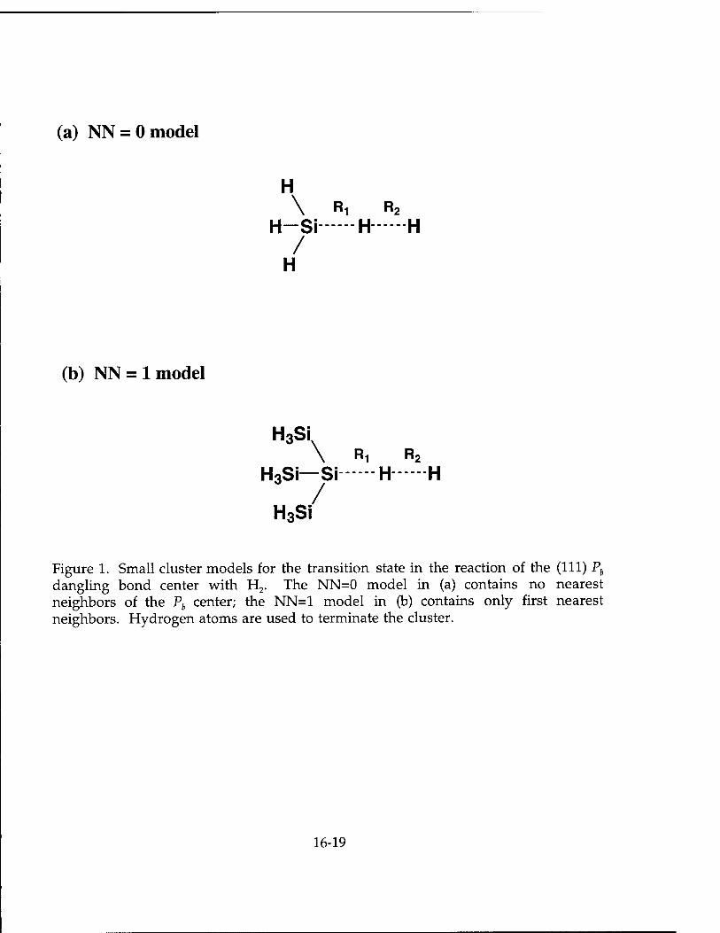
(a) NN = 0 model
H \ R, R2
H-Si H H /
H
(b) NN = 1 model
H3Si \ Rt R2
H3Si—Si H H
H3Si
Figure 1. Small cluster models for the transition state in the reaction of the (111) Pb
dangling bond center with H2. The NN=0 model in (a) contains no nearest neighbors of the Pb center; the NN=1 model in (b) contains only first nearest neighbors. Hydrogen atoms are used to terminate the cluster.
16-19
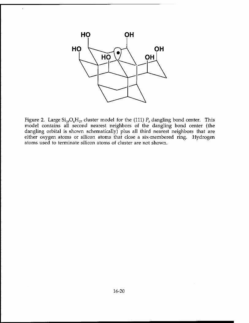
Figure 2. Large Si1906H27 cluster model for the (111) Pb dangling bond center. This model contains all second nearest neighbors of the dangling bond center (the dangling orbital is shown schematically) plus all third nearest neighbors that are either oxygen atoms or silicon atoms that close a six-membered ring. Hydrogen atoms used to terminate silicon atoms of cluster are not shown.
16-20
EXCITATION OF OSCILLATING TWO STREAM INSTABILITY BY UPPER HYBRID PUMP WAVES IN IONOSPHERIC HEATING EXPERIMENTS AT
TROMSO
S. P. Kuo Professor
Department of Electrical Engineering
Polytechnic University Route 110
Farmingdale, New York 11735
Final Report for: Summer Research Program
Phillips Laboratory
Sponsored by: Air Force Office of Scientific Research
Boiling Air Force Base, Washington, DC
And
Phillips Laboratory
August 1997
17-1
Excitation of Oscillating Two Stream Instability by Upper Hybrid Pump Waves in
Ionospheric Heating Experiments at Tromso
S. P. Kuo Professor
Department of Electrical Engineering Polytechnic University
Abstract
It is shown that upper hybrid waves generated by the HF heater wave in the
Tromso' heating experiments can excite oscillating two stream instability near the upper
hybrid resonance layer of the heater wave. The sidebands of the investigated parametric
instability are obliquely propagating Langmuir waves. These Langmuir waves can be
excited in milliseconds and have a broad angular distribution. Thus, those waves
propagating obliquely at small angles with respect to the geomagnetic field can contribute
to the zero off-set frequency component of the plasma line spectrum detected by a
backscatter radar. The analyses also show that the wavelengths of the Langmuir waves
have an upper bound and consequently, explain why the zero off-set frequency plasma line
has been detected by the EISCAT 933 MHz (UHF) radar, but not by the EISCAT 244
MHz (VHF) radar as reported in Stubbe et. al. [1992].
17-2
Excitation of Oscillating Two Stream Instability by Upper Hybrid Pump Waves in
Ionospheric Heating Experiments at Tromso
S. P. Kuo
I. Introduction
During the HF heating of the ionosphere, parametric instabilities can provide
effective channels to convert electromagnetic waves into electrostatic plasma waves with
high and low frequencies [Perkins et al, 1974; Fejer, 1979; Kuo, 1992]. In the midlatitude
region such as Arecibo, Puerto Rico, the instabilities are excited by the o-mode heater
wave near its reflection height [Carlson et al., 1972; Djuth et al., 1990], where the heater
wave electric field is polarized nearly parallel to the geomagnetic field. Thus, the sidebands
of the parametric decay instability (PDI) and oscillating two stream instability (OTSI) are
Langmuir waves, which propagate within a small cone around the geomagnetic field [Fejer
and Kuo, 1973]. By contrast, in the high-latitude region such as Tromso, Norway, the
heater wave can effectively interact with the ionosphere at its upper hybrid resonance
layer, where the o-mode heater wave is still characterized by the right-hand circular
polarization, before the heater wave reaches its reflection height [Stubbe et al., 1982; Lee
and Kuo, 1983; Leyser, 1991]. It has been shown that thermal parametric instabilities [Lee
and Kuo, 1983; Huang and Kuo, 1994] can be effectively excited in this region, and the
sidebands are upper hybrid waves propagating nearly perpendicular to the geomagnetic
field. The upper hybrid waves can also be generated by linear mode conversion of the HF
heater wave [Mjolhus, 1990]. The upper hybrid waves are found to play a key role in the
17-3
generation of" stimulated electromagnetic emissions ( SEEs ) ", observed in Tromso's
heating experiments [Stubbe et al., 1984; Stenflo, 1990; Leyser, 1994; Zhou et al., 1994].
Due to the field-aligned nature of the upper hybrid waves, they can not be detected
by EISCAT's VHF and UHF backscatter radars. However, Langmuir waves referred to as
" HFPLs ", have been detected by EISCAT's UHF and VHF radars during Tromso's
heating experiments [Hagfors et al., 1983; Stubbe et al., 1985; Isham et al., 1990; Stubbe
et al., 1992]. Similar to the Arecibo's situation, these Langmuir waves can be excited by
the o-mode heater wave near its reflection height via the PDI or OTSI processes.
However, these instabilities have to compete with those occuring in the upper hybrid
resonance region located at a lower height and depleting the heater wave power.
Experimental results show that the intensity ratio of the OTSI to decay lines, while
virtually independent of heater power, depends markedly on radar frequency. The OTSI
line is strong as monitored with the EISCAT UHF radar, but very weak or absent with the
EISCAT VHF radar [ Stubbe, et al., 1992].
The present work is aimed at understanding the afore-mentioned observations at
Tromso using the EISCAT's radar facilities. We show that the Langmuir waves at the
heater frequency (viz., OTSI lines) observed in the Tromso's heating experiments can, in
fact, be excited parametrically by the upper hybrid waves. These upper hybrid waves are
excited directly by the o-mode heater wave via either the thermal OTSI process [ Lee and
Kuo, 1983; Huang and Kuo, 1994] or the mode conversion process [Mjolhus, 1990]. In
section II, the theory of the proposed instability process is presented. The fo'rmulation
17-4
includes the derivation of coupled mode equations and the dispersion relation. The
dispersion relation is analyzed in section HI, in which the threshold fields and growth rates
of instabilities for two different decay modes are derived analytically and evaluated
numerically. A comparison of the two instability processes is made to show the dominant
one related to the observations at Tromso. The concluding remarks are finally drawn in
section IV.
17-5
II. Theory
Experiments and theories have shown that upper hybrid waves can be excited by
the HF heater wave near the upper hybrid resonance layer via thermal parametric
instabilities and/or mode conversion in the heating experiments conducted at Tromso,
Norway. After the excited upper hybrid waves grow and acquire sufficiently large
intensities, they become pump waves to excite various parametric instabilities, broadening
the spectral distribution of plasma waves.
In the following we analyze the decay of a field-aligened upper hybrid pump wave
(coi, ki=xki ) into two obliquely propagating Langmuir waves (©o, ko) and ( ©2, k2 ), and
an ion mode ( co9, k=zk ) which is either a purely growing mode or an ion acoustic mode.
The geomagnetic field is chosen to be in the z-direction, ie. Bo=zB0. The process under
consideration can be represented by the following matching relations:
©i = ©2 + oos = ©o - ffls, ki = k2 + k = ko - k
where the wave vector matching conditions are illustrated in Figure 1.
A. Coupled Mode Equations for Obliquely Propagating Langmuir Waves:
The coupled mode equations for Langmuir sidebands (©0, ko; ©2, k2) in terms of
the upper hybrid pump wave ( ©i, ki ) and the ion decay mode ( ©s, k ) can be derived
from the electron continuity equation and electron momentum equation together with
Poisson's equation, as
17-6
{(dt + ve f [ ö,( 5t + ve) + (okt2 ] + a [ 5, (5, + ve) + (k/k,r o)kt ]} <t>o,2
^-(öp^k./kO^Öt+Ve)2 [(|)i(n,o,2/no)] (1)
where <h, <j)o and <t>2 are electric potentials of the upper hybrid pump wave, up-shifted and
down-shifted Langmuir sidebands; n,0 = n, = ns2* is the density perturbation associated
with the ion decay mode and no is the unperturbed electron density; kt = ki + k , cokt =
Qp2 + 3kt2v,e2, vte = (Te/me)172 is the electron thermal speed and cop is the electron plasma
frequency; H« = eB0/mc and ve are the electron cyclotron and collision frequency
respectively.
Assuming that all the physical quantities of the waves involved have a time
harmonic function form, ie., s = sViMt, the coupled mode equations (1) are reduced to
'<Jo,2 = (k,/k,)2(üp2i1(fIso,2/no)/[(k^)2(a2CDkt2/ü)i2-3kt
2vte2)+(ö1(ive±2ü)s„,2)] (2)
where co,0 = cos = ü)S2*; O/W « 1 is assumed.
To complete the description of the considered instability process, a coupled mode
equation relating n, to <j)0,2 is derived as follows.
B. Coupled Mode Equation for the Low Frequency Decay Mode:
The low frequency decay mode is either a purely growing mode (ie. cos = iy) or an
ion acoustic wave (ie. CD, = kCs+ iy, where C, = [(Tc+3Ti)/mi]1/2 is the ion acoustic speed
17-7
). In either case, the wave vector of the decay mode is assumed to be along the
geomagnetic field (ie. k = zk ). The damping mechanisms of these two decay waves are ,
however, quite different. The damping rate of the purely growing mode is proportional to
Vin , the ion-neutral collision frequency, while the ion acoustic wave is heavily damped by
the ion Landau damping process. From ion continuity equation and momentum equation,
the coupled mode equation is derived to be
( <DS2 + ivioo. - k2Cs
2) (n/no) = (m/M) k2 (?„ -v,* + vVv2*) (3)
where v; is the ion-neutral collision frequency Vjn for the purely growing mode and is
twice the ion Landau damping rate 2ri=(7r;/2)1/2ü)s{(m/M)1/2+(Te/Ti)3/2exp[-(Te/2Ti+3/2)]}
for the ion acoustic wave; the coupling term on the right hand side of Eq.(3) is contributed
by the ponderomotive force of high frequency electrostatic waves on the plasma electrons.
Vi, Vo and v2 are the linear velocity responses of electrons to the high frequency
electrostatic wave fields 4>i,d>o and fa respectively. Using the electron continuity equation
and momentum equation, these velocity responses can be determined in terms of the
corresponding wave field. The results are then substituted into Eq.(3), leading to
(Qs2 + ivjco, -k2Cs
2 ) (ris/no) =
(mM){(ekk1(o1/mfflp)2/[fflp2-3k2vte2(l-a2/co,2)]}{(l+a2/(Oi2)($o^r+$ii2V
[(l+2ne2/(ö,2)((ös/(öO+i(l+a2/ü),2)(3kV/fflp
2)(vy(DO](?o?r-$i^)} " (4)
17-8
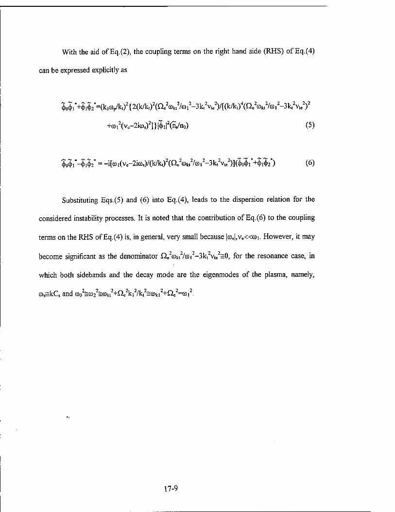
With the aid of Eq.(2), the coupling terms on the right hand side (RHS) of Eq.(4)
can be expressed explicitly as
tti*4i$2*=(k,oA)2{2(k/kt)Wa>ktV
+ö)12(ve-2i(ös)
2]}|^1|2(H5/no) (5)
• , "Y •* <t>o<t>i*—<t>i4>2* = -i[ffli(ve-2i(D5)/(k/kt)
2(n/ü)kt7co12-3kt'vte
Z)]((|)o(l)i +<t>i<t>2 ) (6)
Substituting Eqs.(5) and (6) into Eq.(4), leads to the dispersion relation for the
considered instability processes. It is noted that the contribution of Eq.(6) to the coupling
terms on the RHS of Eq.(4) is, in general, very small because |co,|,vc«a)i. However, it may
become significant as the denominator U.2©kt2/cDi2-3k,2vte2=0, for the resonance case, in
which both sidebands and the decay mode are the eigenmodes of the plasma, namely,
(D^kC, and ©02=co2
2^kt2+^2ki2/kt2=cOki2+ne2=ai2.
17-9
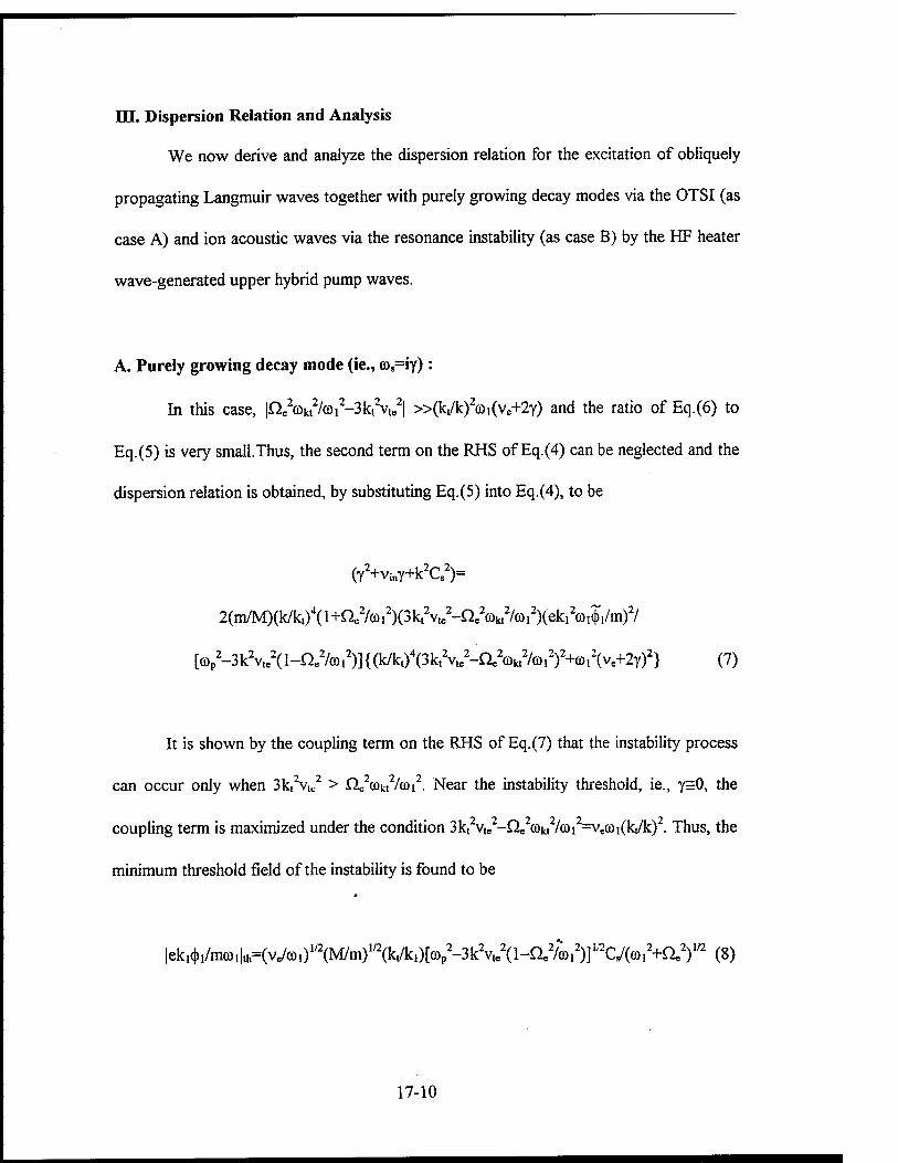
BDE. Dispersion Relation and Analysis
We now derive and analyze the dispersion relation for the excitation of obliquely
propagating Langmuir waves together with purely growing decay modes via the OTSI (as
case A) and ion acoustic waves via the resonance instability (as case B) by the HF heater
wave-generated upper hybrid pump waves.
A. Purely growing decay mode (ie., co,=iy):
In this case, |QeW/coi2-3kt2vte
2| »(k,/k)2a>i(ve+2y) and the ratio of Eq.(6) to
Eq.(5) is very small.Thus, the second term on the RHS of Eq.(4) can be neglected and the
dispersion relation is obtained, by substituting Eq.(5) into Eq.(4), to be
(Y2+VinY+k2C52)=
2(rn/M)(k/kt)4(l+a2/ö)i2)(3kt
2vle2-a2o)kt2/©i2)(ekI
2ü)^,/m)2/
[cDp2-3kV(l-ne
2/ö)i2)]{(k/kt)4(3ktV-a2(Dkt2/ü),2)2+(ö1
2(Ve+2y)2} (7)
It is shown by the coupling term on the RHS of Eq.(7) that the instability process
can occur only when 3kt2Vie
2 > ne2cükt2/ü>i2. Near the instability threshold, ie., y=0, the
ly A ry ry ry ry
coupling term is maximized under the condition 3kt vte -Qe (Akt /©i =vecoi(kt/k) . Thus, the
minimum threshold field of the instability is found to be
lek^/möilth^VcAöO"2^^ (8)
17-10
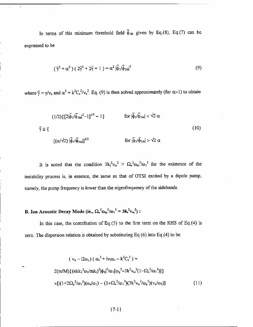
In terms of this minimum threshold field <j>iu, given by Eq.(8), Eq.(7) can be
expressed to be
(f + a2) (2y2 + 2y + 1) = a2 |<{>,A|>uhf (9)
where y = y/ve and a2 = k2C,2/ve2. Eq. (9) is then solved approximately (for a>l) to obtain
(l/2){[2|$,/^,h|2-l]1/2 - 1} for fii/iM < V2 a
y={ (10)
[(a/V2) |$,/^,th|]1/2 for |$,/<i>iih| > ^2 a
It is noted that the condition 3kt2v,e
2 > ne200kt2/©i2 for the existence of the
instability process is, in essence, the same as that of OTSI excited by a dipole pump,
namely, the pump frequency is lower than the eigenfrequency of the sidebands.
B. Ion Acoustic Decay Mode (ie., ne2<ökt2/a>i2 = 3k,2v,e
2):
In this case, the contribution of Eq.(5) to the first term on the RHS of Eq.(4) is
zero. The dispersion relation is obtained by substituting Eq.(6) into Eq.(4) to be
( ve - i2cos) (cos2 + iviOOs - k2Cs
2) =
2(m/M){(ekk,2ü),/rnkt)2|(|),|2/{Dl[cOp2-3k2vte
2(l-a2/coi2)]}
x[i(l+2a2/co,2)((ö5/ü)1) - (l+Oe2/coi2)(3k2vte2/©p
2)(Ve/ü),)] (11)
17-11
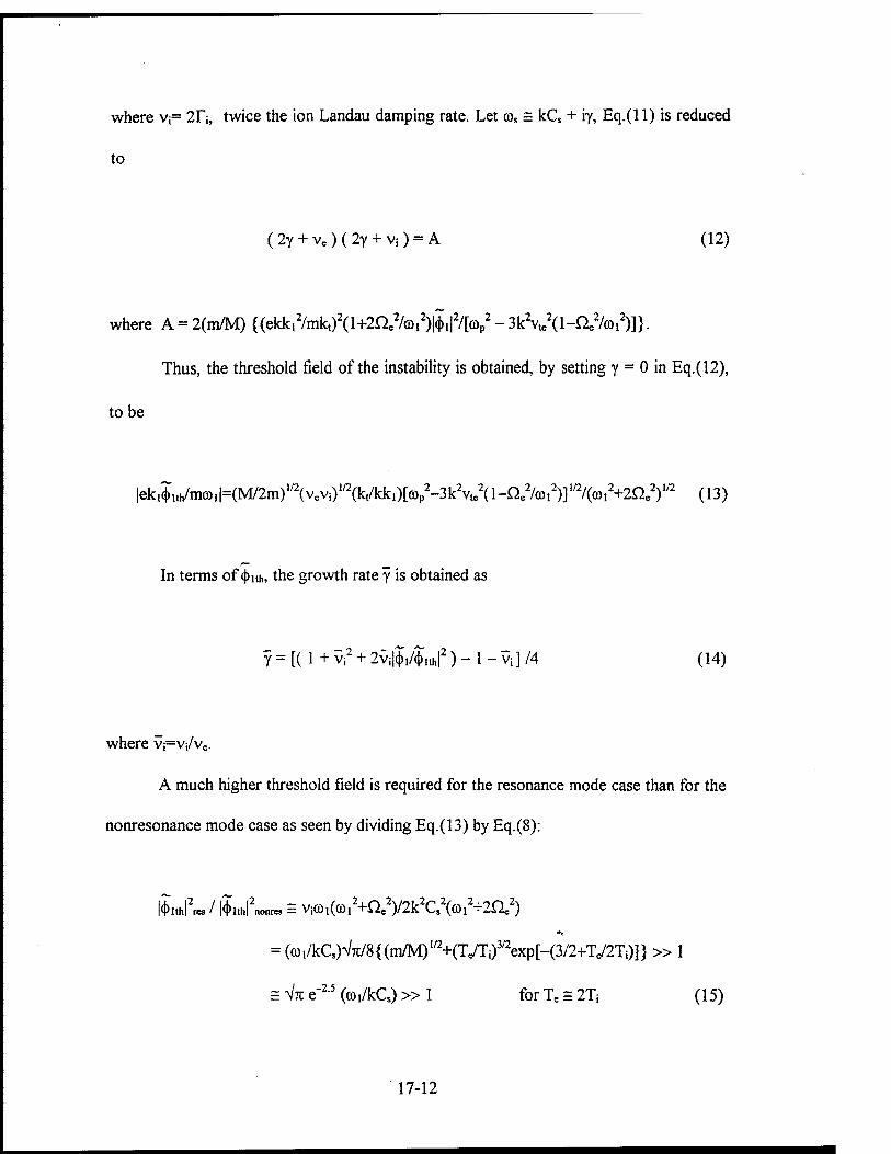
where Vi= 21"*;, twice the ion Landau damping rate. Let cos = kCs + iy, Eq.(H) is reduced
to
(2y + vc)(2Y + Vi) = A (12)
where A = 2(m/M) {(ekk12/mk,)2(l+2a2/©,2)|J,|2/[(Dp
2- 3kV(l-ne2/coi2)]}.
Thus, the threshold field of the instability is obtained, by setting y = 0 in Eq.(12),
tobe
|eki5,ü/m(ü1|=(M/2m)lß(vev01/2(k,/kki)[(Dp2-3kV(l-a2/oi2)]w/(öi2+2a2)1/2 (13)
In terms of (jhu,, the growth rate y is obtained as
y = [( 1 + Vi2 + 2vi|$,Ajlth|2 )-l-Vi]/4 (14)
where Vj=Vi/ve.
A much higher threshold field is required for the resonance mode case than for the
nonresonance mode case as seen by dividing Eq.(13) by Eq.(8):
IW» / iJlthfnonrc = ViO.^+a^k^W+Sfl.2)
= (ffl1/kC,)V7t/8{(m/M)1/2+(Te/Ti)3/2exp[-(3/2+Te/2Ti)]} » 1
= VTC e"2"5 (©,/kCs)» 1 for Te = 2Tj (15)
17-12
Therefore, the instability favorably excited by the upper hybrid pump generates a
nonpropagating purely growing mode as the decay mode. Considering the heating
experiments at Tromso, where the geomagnetic dip angle is about 78°, we adopt the
following parameters for evaluating the threshold field and the growth rate of the
instability: CöI/2TC=4MHZ, £Va>i=l/3, ve=500 s"1, Te=2T;=2000K, v,e=1.8xl05 m/s,
m/M=3.4xlO~5, and C,=1.66xl03 m/s.
The threshold field Eith=|ki<f»ith| calculated from Eq.(8) is found to be
Ellh = 0.15[l+(k/k,)2]1/2 (V/m) (16)
Thus, to convert the field-aligned upper hybrid wave ( propagating perpendicular
to the geomagnetic field) into up- or down-going Langmuir waves ( propagating at 12° to
the geomagnetic field ), it requires k/ki=cotl2°=4.7 and the threshold field obtained from
Eq.(16) is about 0.7 V/m. Assuming that Ei = |ki<j>i| = 1 V/m, the growth rate of the
Langmuir waves propagating vertically (ie., having k/ki = 4.7) is obtained from Eq.(10) to
be about 190 s"1, ie., y = 0.38. Those Langmuir waves with k/ki < 4.7 have lower
threshold fields and thus, higher growth rates. For example, Langmuir waves propagating
at 45° with respect to the geomagnetic field have k/ki=l and thus, Elth=0.212 V/m and
y=1.4xl03 s"1 (or Y=2.8). However, those Langmuir waves propagate obliquely to the
vertical direction and thus, are unable to be detected by the backscatter radars.
"Because case A is the dominant process, thus, the frequencies of the excited
Langmuir waves are the same as those of the upper hybrid pump waves, which are
17-13
identical to the heater wave frequency. As afore-mentioned, the case A process can only
occur when 3kt2vte
2 > £Se2o)kt2/coi2 = He2. Substituting the parametric values into this
inequality, it leads to Xi < 0.23 m. Since the wavelengths of the plasma lines detected by
EISCAT 933 MHz UHF and 224 MHz VHF radars are 0.161 m and 0.67 m respectively,
it explains why the EISCAT UHF radar has detected the ' OTSI line" ( ie. zero off-set
frequency line), while the EISCAT VHF radar has not [see Stubbe et al., 1992].
17-14
IV. Conclusion
A parametric instability process which renders the decay of an upper hybrid pump
wave into two obliquely propagating Langmuir sidebands and a purely growing mode is
studied. The results show that the Langmuir waves can be excited in milliseconds and have
a broad angular distribution. However, the wavelengths of the Langmuir waves are limited
to Xt < 0.23 m. Thus, the proposed process can be based on to understand why the
EISCAT 933 MHz backscatter radar ( half wavelength=0.161 m < 0.23 m) but not the
244 MHz radar ( half wavelength=0.67 m > 0.23 m) can detect the Langmuir waves which
have a zero off-set frequency [Stubbe et al., 1992].
The other outstanding feature observed at Tromso is that the intensity ratio of the
OTSI plasma lines to the PDI lines is virtually independent of the input heater power. The
OTSI lines are radar-detected Langmuir waves with zero off-set frequency from the heater
wave frequency, while the PDI lines are those with frequencies off-set from the heater
wave frequency by the ion acoustic wave frequency. This feature can be understood by
means of the following facts : (1) the upper hybrid pump waves producing the OTSI lines
can be generated by the HF heater wave via the mode conversion process [Mjolhus,
1990], which requires no threshold, and (2) the threshold of the PDI process can be easily
exceeded in Tromso experiments. In other words, both the OTSI plasma lines and the PDI
lines can be produced by rather low heater power. Consequently, the intensity ratio of the
OTSI to PDI lines is not sensitive to the variation of the heater power. In the present
work, the wave vectors of the excited purely growing (ie., zero-frequency) modes are
17-15
modes propagating at a small but finite angle with respect to the geomagnetic field can
also be excited by the upper hybrid waves. These obliquely propagating, namely, zero-
frequency modes can contribute to the zero-frequency component ( known as the central
line) of the ion line spectrum detected by the EISCAT UHF ( 933 MHz) radar [Stubbe et
al., 1992].
Acknowledgments
The author gratefully acknowledges useful discussions with M. C. Lee, Keith
Groves, Ed Weber, Paul Kossey, and John Heckscher. This work was completed at the
Air Force Phillips Laboratory, Hanscom AFB, Massachusetts, whose hospitality is
appreciated.
17-16
References
Carlson, H. C, W. E. Gordon, and R. L. Showen, High-frequency induced enhancements
of the incoherent scatter spectrum at Arecibo, J. Geophys. Res., 77, 1242, 1972.
Diuth, F. T., M. P. Sulzer, and J. H. Elder, High-resolution observations of the HF-
induced plasma waves in the ionosphere, Geophys. Res. Lett., 17, 1893, 1990.
Fejer, J. A., Ionospheric modification and parametric instabilities, Rev. Geophys., 17, 135,
1979.
Fejer, J. A. and Y. Y. Kuo, Structure in the nonlinear saturation spectrum of parametric
instabilities, Phys. Fluids, 16, 1490, 1973.
Hagfors, T., W. Kofman, H. Kopka, P. Stubbe, and T. Aijanen, Observations of enhanced
plasma lines by EISCAT during heating experiments, Radio Sei., 18, 861, 1983.
Huang, J. and S. P. Kuo, Cyclotron harmonic effect on the hermal oscillating two-stream
instability in the high latitude ionosphere, J. Geophys. Res., 99, 2173, 1994.
Isham, B., W. Kofman, T. Hagfors, J. Nordling, B. Thide, C. LaHoz, and P. Stubbe, New
phenomena observed by EISCAT during an RF ionospheric modification
experiment, Radio Sei., 25, 251, 1990.
Kuo, S. P.,Criteria for excitation of parametric instability in the ionosphere by an obliquely
incident high-frequency heater, Phys. Fluids B, 4, 1012, 1992.
Lee, M. C. and S. P. Kuo, Excitation of upper hybrid waves by a thermal parametric
instability, J. Plasma Phys., 30, 463, 1983.
Leyser;>T. B., Parametric interaction between upper hybrid and lower hybrid waves in
heating experiments, Geophys. Res. Lett., 18, 408, 1991.
17-17
Leyser, T. B., Electromagnetic radiation by parametric decay of upper hybrid waves in
ionospheric modification experiments, Phys. Plasmas,l, 2003, 1994.
Mjolhus, E.,On linear conversion in .a magnetized plasma, Radio Sei., 25, 3121, 1990.
Perkins, F. W., C. Oberman, and E. J. Valeo, Parametric instabilities and ionospheric
modification, J. Geophys. Res., 79, 1478, 1974.
Stenflo, L., Stimulated scattering of large amplitude wave in the ionosphere, Phys. Scr.,
T30, 166, 1990.
Stubbe, P., H. Kopka, T. B. Jones, and T. Robinson, Wideband attenuation of radio
wavescaused by powerful HF waves: saturation and dependence on ionospheric
variability, J. Geophys. Res., 87, 1151, 1982.
Stubbe, P., H. Kopka, B. Thide, and H. Derblom, Stimulated electromagnetic emission: a
new technique to study the parametric decay instability in the ionosphere, J.
Geophys. Res., 89, 7523, 1984.
Stubbe, P., et al., Ionospheric modification experiments with the Tromso heating facility,
J. Atmos. Terr. Phys., 47, 1151, 1985.
Stubbe, P., H. Kohl, and M. T. Rietveld, Langmuir turbulence and ionospheric
modification, J. Geophys. Res., 97, 6285, 1992.
Zhou, H. L., J. Huang, and S. P. Kuo, Cascading of the upper hybrid/electron Bernstein
wave in the ionospheric heating experiments, Phys. Plasmas, 1, 3044,1994.
17-18
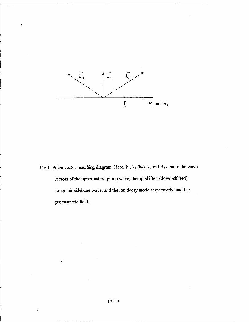
k B0 — zB0
Fig. 1 Wave vector matching diagram. Here, ki, ko (k2), k, and B0 denote the wave
vectors of the upper hybrid pump wave, the up-shifted (down-shifted)
Langmuir sideband wave, and the ion decay mode,respectively, and the
geomagnetic field.
17-19
H2 REACTIONS AT DANGLING BONDS IN SI02
Henry A. Kurtz Professor
Department of Chemistry
University of Memphis Memphis, TN 36152-6060
Final Report for: Summer Research Program
Phillips Laboratory
Sponsored by: Air Force Office of Scientific Research
Boiling Air Force Base, Washington, DC
And
Phillips Laboratory
September 1997
18-1
H2 REACTIONS AT DANGLING BONDS IN SI02
Henry A. Kurtz Professor
Department of Chemistry University of Memphis
Abstract
The hydrogen passivation reaction at the dangling bond on an E' center in Si02 is studied using the model reaction H2 +-Si(OH)3 -> -H + HSi(OH)3. A study of the energetics of this reaction at the Hartree-Fock and MP2 level is presented with a variety of basis sets. Direct dynamics calculations are also performed to evaluate rate constants and activation energies for the process, with and without the inclusion of quantum tunneling effects. The results are compared to an experimental value for the activation energy of H2 annealing of E' centers.
18-2
H2 REACTIONS AT DANGLING BONDS IN SI02
Henry A. Kurtz
I. INTRODUCTION
The passivation of reactive defects due to unfilled valences of Si atoms (called dangling bonds) in
amorphous silicon dioxide by H2 is thought to proceed via the reaction
H2 + -Si= -» -H + HSi=
where the symbol = represents the three satisfied valences (bonds).1 This is a very general reaction that may take
place both at the Si/Si02 interface and in bulk Si02. At the interface the three bonds are to other silicon atoms and
the defect is known as a Pb center. In the bulk Si02 the three bonds are to oxygen atoms and is part of an E'
center. It is the these latter defects that will be the focus of this work.
Hydrogen annealing of E* centers has been studied by Li et al.\ They used ESR measurements of E'
center concentrations to estimate rate constants and an activation energy for the annealing process. The activation
energy they obtained is 0.3 eV and was attributed to a process like the one shown above. However, the experiment
is not really able to identify the actual molecular processes for which the activation energy was measured. An
alternate explanation for this results could be the measured activation energy is due to H2 complexation or some
other physical process. The activation associated with diffusion of H2 in amorphous Si02 is 0.38 eV, about the
same size.3 Edwards4,1 performed Hartree-Fock calculations on model systems to estimate an activation energy for
this process of around 0.7 eV - much larger than the experimental value. Edwards further suggested that the
discrepancy may arise because quantum tunneling effects were not included. He estimated that the tunneling
corrections may lower the theoretical activation energy to about 0.1 eV - now much lower than Li et al 's
experiment. The goal of this Summer Faculty Research project is to re-examine the theoretical methods and models for
H2 reactions with Si dangling bonds in Si02 and to calculate rate constants for this process via direct dynamics,
with and without tunneling.
II. ENERGETICS
The first model studied in this work for the reactions is the small cluster reaction:
H2 + -Si(OH)3 -> -H + HSi(OH)3
18-3
which is one of the cluster models used by Edwards.4 The energetics of the model reaction is studied by calculating
the molecular structure and energies of the reactants and products. The reactants and products are characterized by
having all positive harmonic vibrational frequencies (i.e., all positive second derivatives of the energy with respect
to atomic motion). The energetic barrier to the reaction is found by calculating the molecular structure and energy
corresponding to the highest point on the minimum energy pathway connecting the reactants and products. This
oint is called the transition state or transition structure (TS). The transition structure corresponds to a saddle point
on the potential energy surface and is characterized by having one, and only one, imaginary vibrational frequency
(i.e., having one negative eigenvalue of the matrix of energy second derivatives).
This model is small enough that a good test of the methods for obtaining energies and structures can be
performed. Initially, for each of the reactants, products, and transition structure, the molecular structures were
optimized using the unrestricted Hartree-Fock method (UHF) for the radical, open-shell species and restricted
Hartree-Fock (RHF) for the closed shell species. The 6-3 IG** one-electron basis set was used.5 This is a standard
split-valence basis set augmented by polarization functions on all atoms (d-functions on the Si and O atoms and p-
functions on the H atoms). For this study, the 6-3 IG** basis set used for Si was the one developed by Gordon and
co-workers.6 The resulting structures for -Si(OH)3, HSi(OH)3, and H-H-Si(OH)3 are shown in Figure 1. This
model differs from the previous same sized model of Edwards3 in that no artificial symmetry was imposed. Each
of the species other than H and H2 are of Cl point group symmetry (i.e., no symmetry constraints). At this level of
theory, the energy of the reaction (EproducU - Ereactanu) is -0.017 eV (-0.402 kcal/mole) - slightly exothermic. The
activation energy for the reaction calculated as the energy difference ETS - ErcacUmU is 0.795 ev (18.341 kcal/mole).
This value is considerably larger than the value of 0.3 eV obtained for the experiment of Li, et al.2
The first goal of this research project was to explore reasonable improvements in the methods used. Table
1 shows the energy of reaction obtained using improved one-electron basis sets and/or adding electron correlation
effects via second-order Moller Plesset perturbation theory (MP2). In this table and the rest of this report, the
notation Method 1 (basis l)//Method2(basis2) refers to calculations done using method 1 (either Hartree-Fock or
MP2) with basis set 1 at an optimized geometry obtained from method 2 with basis set 2. For example, MP2(6-
31G**++)//UHF(6-31G**) uses energies obtained from an MP2 calculation using the 6-31G**++ basis set with
the molecular geometries from an UHF calculation using a 6-3 IG** basis set. The structure and energy results
presented in this report were obtained using the GAMESS7 and GAUSSIAN948 programs.
18-4
Si(OH),
H-H-Si(OH)3
HSi(OH),
Figure 1
18-5

Table 1: Reaction Energies for H2 + -Si(OH)3 ■» -H + HSi(OH)3
UHF(6-3 lG**)//UHF(6-3 IG**) UHF(6-31 lG**)//UHF(6-3 IG**) UHF(6-3 lG**++)/UHF(6-3 IG**)
UHF(6-3 lG**)//MP2(6-3 IG**) UHF(6-3 lG**++)/MP2(6-3 IG**)
MP2(6-3 lG**)//UHF(6-3 IG**) MP2(6-31 lG**)//UHF(6-3 IG**) MP2(6-3 lG**++)/UHF(6-3 IG**)
MP2(6-31G**)//MP2(6-31G**) MP2(6-31G**++)/MP2(6-31G*'t')
-0.0006405 a.u. -0.0024469 a.u. 0.0022961 a.u.
-0.0008755 a.u. 0.0020546 a.u.
0.0068737 a.u. 0.0036013 a.u. 0.0097772 a.u.
0.0070781 a.u. 0.0101345 a.u.
-0.017 eV -0.067 eV 0.062 eV
-0.024 eV 0.056 eV
0.187 eV 0.098 eV 0.266 eV
0.193 eV 0.276 eV
-0.402 kcal/mole -1.535 kcal/mole 1.441 kcal/mole
-0.549 kcal/mole 1.289 kcal/mole
4.313 kcal/mole 2.260 kcal/mole 6.135 kcal/mole
4.442 kcal/mole 6.360 kcal/mole
Basis set improvements, as illustrated by the first three rows of Table 1, have contradictory effects but the
magnitudes are very small. In the 6-31 IG** basis set, the size of the one-electron basis used to describe the
valence shell is increased and, in the 6-31G**++ basis set, extra diffuse functions were added to each atom.
Calculations on the combined basis set (6-311G**++) are underway currently. The inclusion of electron
correlation at the MP2 level has a larger effect on the results - changing the essentially energy neutral reaction into
definitely being endothermic. However, the resulting reaction energy is still quite small. Table 1 also illustrates
that the overall energetics of this reaction are not particularly sensitive to geometry - results based on UHF
structures agree quite well with results based on MP2 structures. Allendorf el al.9 obtained an MP4/6-31G*
estimate of AH°(298K) of 3.30 kcal/mole, close to the MP2 estimate here. Further improvements in the theory
maybe be needed to refine the reaction energy but no significant change is expected.
The main quantities of interest in this study are the activation energies for the reaction of H2 + 'Si(OH)3
and these results are shown in Table 2. The important tiling to note is that there is very little variation in the
computed activation energy with improvements in the basis sets or with the inclusion of electron correlation. It
seems very unlikely that making further improvements of this type will change the activation barrier out of the
0.7-0.8 eV range - still quite far from the experimental value of 0.3 eV.
Table 2. Activation Energy for H2 + -Si(OH)3 UHF(6-31G**)//UHF(6-31G**) UHF(6-31 lG**)//UHF(6-3 IG**) UHF(6-31G* *++)/UHF(6-31G**)
UHF(6-31G**)//MP2(6-31G**) UHF(6-31G**++)//MP2(6-31G**)
MP2(6-3 lG**)//UHF(6-3 IG**) MP2(6-31 lG**)//UHF(6-3 IG**) MP2(6-31G**++)/UHF(6-31G**)
MP2(6-3 lG**)//MP2(6-3 IG**) MP2(6-31G**++)//MP2(6-31G**)
0.0292279 a.u. 0.795 eV 18.341 kcal/mole 0.0277876 a.u. 0.756 eV 17.437 kcal/mole 0.0320129 a.u. 0.871 eV 20.089 kcal/mole
0.0288851 a.u. 0.786 eV 18.126 kcal/mole 0.0316718 a.u. 0.862 eV 19.874 kcal/mole
0.0272257 a.u. 0.741 eV 17.084 kcal/mole 0.0230080 a.u. 0.626 eV 14.438 kcal/mole 0.0294786 a.u. 0.802 eV 18.498 kcal/mole
0.0274339 a.u. 0.747 eV 17.215 kcal/mole 0.0292858 a.u. 0.797 eV 18.377 kcal/mole
18-6
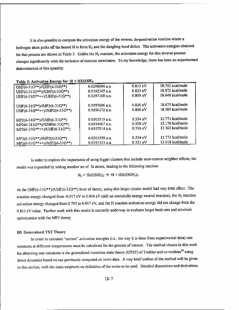
It is also possible to compute the activation energy of the reverse, de-passivation reaction where a
hydrogen atom picks off the bound H to form H2 and the dangling bond defect. The activation energies obtained
for this process are shown in Table 3. Unlike the H2 reaction, the activation energy for this reverse process
changes significantly with the inclusion of electron correlation. To my knowledge, there has been no experimental
determination of this quantity.
Table 3: Activation Energv for -H + HSi(OH)3
UHF(6-3 lG**)//UHF(6-3 IG**) UHF(6-31 lG**)//UHF(6-3 IG**) UHF(6-31G**++)/UHF(6-31G**)
0.0298684 a.u. 0.0302345 a.u. 0.0297168 a.u.
0.813 eV 0.823 eV 0.809 eV
18.742 kcal/mole 18.972 kcal/mole 18.648 kcal/mole
UHF(6-31G**)//MP2(6-31G**) UHF(6-31G* *++)//MP2(6-31G* *)
0.0297606 a.u. 0.0296172 a.u.
0.810 eV 0.806 eV
18.675 kcal/mole 18.585 kcal/mole
MP2(6-31G* *)//UHF(6-31G**) MP2(6-31 lG**)//UHF(6-3 IG**) MP2(6-3 lG**++)/UHF(6-3 IG**)
0.0203519 a.u. 0.0194067 a.u. 0.0197014 a.u.
0.554 eV 0.528 eV 0.536 eV
12.771 kcal/mole 12.178 kcal/mole 12.363 kcal/mole
MP2(6-31G**)//MP2(6-31G**) MP2(6-3 lG**++)//MP2(6-3 IG**)
0.0203558 a.u. 0.0191513 a.u.
0.554 eV 0.521 eV
12.773 kcal/mole 12.018 kcal/mole
In order to explore the importance of using bigger clusters that include next-nearest neighbor effects, the
model was expanded by adding another set of Si atoms, leading to the following reaction
H2 + -Si(OSiH3)3 ■> -H + HSi(OSiH3)3
At the UHF(6-3 lG**)//UHF(6-3 IG**) level of theory, using this larger cluster model had very little effect. The
reaction energy changed from -0.017 eV to 0.004 eV (still an essentially energy neutral reaction), the H2 reaction
activation energy changed from 0.795 to 0.817 eV, and the H reaction activation energy did not change from the
0.813 eV value. Further work with this model is currently underway to evaluate larger basis sets and structure
optimization with the MP2 theory.
III. Generalized TST Theory
In order to calculate "correct" activation energies (i.e., the way it is done from experimental data) rate
constants at different temperatures must be calculated for the process of interest. The method chosen in this work
for obtaining rate constants is the generalized transition state theory (GTST) of Truhlar and co-workers10 using
direct dynamics based on our previously computed ab initio data. A very brief outline of the method will be given
in this section, with the main emphasis on definition of the terms to be used. Detailed discussions and derivations
18-7
of GTST can be found elsewhere.10 All dyanmics (rate contant) calculations presented here were done with the
POLYRATE program.11
Conventional transition state theory (TST) calculates the thermal rate constants by assuming that all
transition state species came directly from reactants and will be converted into products. The rate is then the flux
across a surface in phase space in the product direction. This rate is given by
km_^Q(I)e-ßv k(1)-ßh<D(T)e
where ß is (kaT)"1, h is Planck's constant, Q(T) is the conventional transition state classical partition function with
its zero of energy at the saddle point, <D(T) is the reactants classical partition function with its zero of energy at the
overall zero of energy, and V is the energy of the saddle point relative to the overall zero of energy.
The generalized transition state theory rate constant is obtained by varying the position of the dividing
surface along the minimum energy path to minimize the value of the computed rate constant.
kGT(T) = minkGT(T,s) = kGT(T,sCVT(T))
where
k (r'S)_ßh O(T) C
Results from this generalized treatment will be referred to as canonical variational theory (CVT). CVT
corresponds to a maximum free energy of activation and includes both "entropic" and energetic effects and has
been demonstrated to be more accurate than TST.
To obtain TST and CVT rate constants all that is needed are the partition functions Q and <t>. In this
work, the separable, harmonic approximation is used which neglects that couplings between the electronic,
vibrational, and rotational energies. The partition function can then be written as
Q(T,s) = Qei(T,s)Qvib(T,s)Qrot(T,s).
The formulas for each of these partition functions are discussed in detail in reference 10. Using only one electronic
surface, Qei depends on the degeneracy of the electronic state, Qvib depends on the harmonic vibrational
frequencies, and Qrot depends on the moments of inertia. All these quantities are easily calculated from the
structural and energetic data discussed previously.
The above two methods give a hybrid treatment of the rate constant in that motion in the degrees of
freedom orthogonal to the reaction path are treated quantum mechanically and motion along the reaction path is
treated classically - neglecting quantum tunneling effects. This means that kCVT often underestimates the rate,
particularly at low temperatures. One way to include quantum reaction path effects is via a multiplicative
transmission coefficient as kCTOY(T) = KCVT/Y(T)kCVT(T)
18-8

For the reactions studied in this work, the method chosen for obtaining the K factors is the small reaction-
path curvature method.10,12 In this method the K factor is calculated via
rP(E)e-E/kBTdE ,rr^ Jo
K(T) = — | e_E/kBTdE JE.(T)
where E*(T) is the quasiclassical ground-state threshold energy. The approximation for P(E) used in this work is
the centrifugal-dominant small-curvature adiabatic ground-state approximation (SCT), which gives
where 0(E) is the imaginary action integral evaluated along the tunneling path,
6(E) = vf V2^ff(s)|E-Va(s)|ds
where Si and Sr are the reaction coordinate turning points.
A detailed description of this procedure is given by references 10 and 12. The essential feature is that
centrifugal effect is included by replacing the reduced mass by an effective reduced mass, ^s) in the action
integral. A special case of the SCT approximation is call the zero-curvature tunneling approximation (ZCT) and is
obtained by setting n*n(s) equal to u. The effect of this is to include tunneling only along the minimum energy
path.
IV. Dynamics Results
In order to perform the direct dynamics calculations including tunneling as discussed above, many points
along the internist reaction coordinate (IRC) [also know as the minimum energy path (MEP)] are needed."
Examples of direct dynamics calculations are given for the reaction OH + HC1 -> Cl + H214 and the similar
reaction CH4 + H -> CH3 + H2". The large computational effort for direct dynamics comes from the fact that at
each point along the IRC, the geometry, potential energy, energy gradient vector and the hessian (energy second-
derivative) matrix is needed. In the present study 83 points were used along the IRC - the reactants, the products,
the TS, and 40 points on each side of the TS. The calculated potential energy along the IRC is shown in Figure 2.
The reaction coordinate is a mass-weighted cartesian coordinate and is arbitrarily set to + toward the reactants and
- toward the products.
18-9
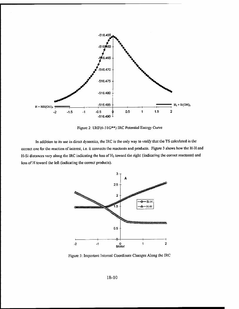
-516.455
H + HSi(OH): H2 + Si(OH)3
Figure 2: UHF(6-31G**) IRC Potential Energy Curve
In addition to its use in direct dynamics, the IRC is the only way to verify that the TS calculated is the
correct one for the reaction of interest, i.e. it connects the reactants and products. Figure 3 shows how the H-H and
H-Si distances vary along the IRC indicating the loss of H2 toward the right {indicating the correct reactants) and
loss of H toward the left (indicating the correct products).
3-
2.5-
2 -
0.5 -
9-
A
—e— Si-H
—A—H-H
I 1 1 1
0 Stotal
Figure 3: Important Internal Coordinate Changes Along the IRC
18-10
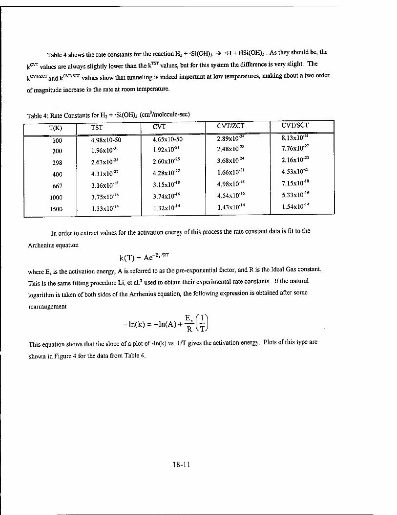
Table 4 shows the rate constants for the reaction H2 + -Si(OH)3 -* -H + HSi(OH)3. As they should be, the
kCVT values are always slightly lower than the kTST values, but for this system the difference is very slight. The
kcvT/zcr and kcvT/scr values ghow ^ tunneling js indeed important at low temperatures, making about a two order
of magnitude increase in the rate at room temperature.
Table 4: Rate Constants for H2 + -Si(OH)3 (cm3/molecule-sec)
T(K) TST CVT CVT/ZCT CVT/SCT
100 4.98x10-50 4.65x10-50 2.89xl0'34 8.13xl0-31
200 1.96xl031 1.92xl0-31 2.48xl0-28 7.76xl0-27
298 2.63xl0-25 2.60xl0-25 3.68xl02" 2.16X10⁻²³
400 4.31xl0"22 4.28xl0"22 1.66xl0-21 4.53xl0"21
667 3.16xl0-'8 3.15X10"18 4.98xl0"18 7.15X10"18
1000 3.75xl0-16 3.74xl0"16 4.54xl0"16 5.33xl0"16
1500 1.33xlOM 1.32xl0'M 1.43xl0-M 1.54xl0"14
In order to extract values for the activation energy of this process the rate constant data is fit to the
Arrhenius equation
k(T)=Ae-E'/RT
where Ea is the activation energy, A is referred to as the pre-exponential factor, and R is the Ideal Gas constant.
This is the same fitting procedure Li, et al.2 used to obtain their experimental rate constants. If the natural
logarithm is taken of both sides of the Arrhenius equation, the following expression is obtained after some
rearrangement
-ln(k) = -ln(A) + ^(^
This equation shows that the slope of a plot of -ln(k) vs. 1/T gives the activation energy. Plots of this type are
shown in Figure 4 for the data from Table 4.
18-11
80
70-
60
£• 50
40
30 -
20
1000/T
Figure 4: Plot of-ln(k) vs. 1000/T
The value of the activation energy obtained from plots like these in Figure 4 clearly depend on the
temperature range used to fit to the -ln(k) vs. 1/T equation. It is most obvious in the CVT/ZCT and CVT/SCT
plots that the slope of the line increases with increasing T (decreasing 1/T) and, therefore, the activation energy
increases as a function of temperature. The experiments of Li et al.2 used data over the temperature range of 23 C
to 299 °C (296 K -473 K), so for comparison the range 298 K - 400 K will be used to extract activation energy
estimates. A summary of activation energy results for the reaction of H2 + *Si(OH)3 are shown in Table 5.
Table 5: Activation Energies for H2 reaction
Method Ea(eV) E„ (kcal/mole)
X^TS " -Lreactants 0.80 18.34
ETS " Ereactanu + ZPE 0.75 17.25
TST 0.75 17.19
CVT 0.75 17.20
CVT/ZCT 0.62 14.21
CVT/SCT 0.54 12.41
Experiment 0.3 6.9
18-12
The best direct dynamics estimate of 0.54 eV is indeed smaller than the .75 eV value obtained only from
the energetics of the stationary points on the potential energy surface but is still larger than the 0.3 eV
experimental quantity.
The rate and activation energy data is also obtained for the reverse reaction of -H + HSi(OH)3 and this
data is shown in Tables 6 and 7. These results indicate that, at the UHF(6-31G**) level, the reverse reaction is of
parable rate to the H2 + -Si(OH)3 reaction and that the activation energy for this process is also similar. comi
Table 6: Rate Constants for -H + HSi(OH)3 (cm3/molecule-sec)
T(K)
100
200
298
400
667
1000
1500
TST
5.55xl0"50
2.04xl0"30
6.80xl024
1.89xl0"20
2.62xl0"16
3.97xl0-14
1.44xl0-12
CVT
5.18xl0'50
2.00xl0-30
6.73xl0'24
1.88xl0-20
2.61xl0'16
3.96xlO-M
1.44xl0-12
Table 7: Activation Energies H Reaction
CVT/ZCT
3.23xl0-34
2.59xl0'27
9.51x10 23
7.32xl0"20
4.13xl0'16
4.81xl0'14
1.56xl0"12
CVT/SCT
9.08xl0"31
8.12xl0"26
5.59xl0"22
1.99X10"19
5.93xl0-16
5.65xl0"14
1.58X10"12
Method Ea(eV) Ea (kcal/mole)
■C-TS " ^reactants 0.81 18.74
ETS - Ereactanü + ZPE 0.77 17.85
TST 0.80 18.42
CVT 0.80 18.43
CVT/ZCT 0.67 15.43
CVT/SCT 0.59 13.64
Since structural and energetic information has been calculated for the reactants, products, and transition
structure at the MP2(6-31G**) level, correlation effects on the rate constant and activation energy at the TST level
have been computed and are shown in Table 8. The MP2 rates are much faster than the corresponding UHF rates
but the activation energy for the H2 + -Si(OH)3 process only slightly lowered. The activation energy for the reverse
•H + HSi(OH)3 process, however shows a significant lowering at the TST level. Clearly, the tunneling calculations
are needed. However, based on the fact that the imaginary frequency of the MP2 transition structure is of smaller
18-13
magnitude than the imaginary frequency of the UHF transition structure, the reaction barrier is wider (smaller
curvature) at the top and the tunneling effects should be smaller, at least at higher temperatures.
Table 8: TST data from MP2(6-31G**) Calculations
H2 + -Si(OH)3 •H + HSi(OH)3
Temperature (K) Rate Constant (cm3/molecule-sec) Rate Constant (cm3/molecule-sec)
100 1.03X10"46 2.29xl036
298 1.18xl0-23 8.25xl0"19
400 1.18xl020 1.82xl0-16
667 4.84xl0-17 1.29xl0"13
1000 4.31xl0-15 4.43xl0-12
1500 1.26xl0"13 5.95x10""
Activation Energy (eV) 0.70 0.54
Table 9 shows some preliminary results at the TST level for the model reaction with a larger cluster. The
results are nearly the same as the smaller cluster which indicates that simply increasing the size of the cluster by
adding next-nearest neighbors has little effect on the chemistry.
Table 9: TST data from UHF(6-3 IG**) Calculations
H2 + -Si(OSiH3)3 •H + HSi(0 SiH3)3
Temperature (K) Rate Constant (cm3/molecule-sec) Rate Constant (cm3/molecule-sec)
100 5.22xl0"51 2.75X10-50
200 6.86xl032 1.16xl030
298 1.38xl0"25 4.02xl0"24
400 2.80xl022 1.14xl0"20
667 2.63xl0'18 1.62xl0-16
1000 3.54xl0-16 2.49xlO"M
1500 1.36xlO-M 9.12xl0"13
Activation Energy (eV) 0.77 0.80
V. Conclusions
This study presented a method for obtaining activation energies that can be used to examine model
reactions which are used to interpret experimental data. With respect to the model reaction
18-14
H2 + -Si(OH)3 -> -H + HSi(OH)3
the inclusion of tunneling effects at the UHF(6-31G**) level of calculation lowered the activation energy toward
the experimental value but a sizable discrepancy still exists.
Current work is underway to continue this study and future work is planned. For the model reaction
above, the direct dynamics including tunneling based on an IRC from a method with electron correlation (at least
at the MP2 level) needs to be done. In addition, further benchmark calculations at a higher level of theory need to
be done to firmly establish the relative energies of the reactants, products, and transition structure. The next steps
in modeling the reaction of H2 at E' centers is to develop better model system that include important interaction in
bulk Si02 that are missing in the current cluster picture - such as nearby non-bonded oxygen atoms and the
positive charged part of the E' center. The thermodynamics and kinetics of reactions at other sites (such as the
positively charged centers) are also planned.
VI. Acknowledgments
RDL and AFOSR are gratefully acknowledged for supporting this work. I would also like to thank all the
people at Phillips lab for making this a very productive period. The Maui HPCC is also acknowledged for
computer support - without which most of these calculations could not have been performed.
V. References
1. A. H. Edwards, J. A. Pickard, and R E. Stahlbush, J. Non-Cryst. Solids 179, 148 (1994).
2. Z. Li, S. J. Fonash, E. H. Poindexter, M. Harmatz, F. Rong and W. R Buchwald, J. Non-Cryst. Solids 126, 173
(1990).
3. J. E. Shelby, J. Appl. Phys. 48, 3387 (1977).
4. A. H. Edwards, J. Non-Cryst. Solids 187, 232 (1995).
5. R. Ditchfield, W. J. Hehre, J. A. Pople, J. Chem. Phys. 54, 724 (1971); W. J. Hehre, R Ditchfield, J. A. Pople,
J. Chem. Phys. 56, 2257 (1972).
6. M. S. Gordon Chem. Phys. Lett. 76, 163 (1980).
7. M. W. Schmidt, K. K. Baldridge, J. A. Boatz, S. T. Elbert, M. S. Gordon, J. H. Jensen, S. Koseki, N.
Matsunaga, K. A. Nguyen, S. J. Su, T. L. Windus, M. Dupuis, J. A. Montgomery, J. Comput. Chem. 14,
1347(1993)
8. Gaussian 94, Revision E.2, M. J. Frisch, G. W. Trucks, H. B. Schlegel, P. M. W. Gill, B. G. Johnson, M. A.
Robb, J. R. Cheeseman, T. Keith, G. A. Petersson, J. A. Montgomery, K. Raghavachari, M. A. Al-Laham, V.
G. Zakrzewski, J. V. Ortiz, J. B. Foresman, J. Cioslowski, B. B. Stefanov, A. Nanayakkara, M. Challacombe,
C. Y. Peng, P. Y. Ayala, W. Chen, M. W. Wong, J. L. Andres, E. S. Replogle, R. Gomperts, R. L. Martin, D.
18-15
J. Fox, J. S. Binkley, D. J. Defrees, J. Baker, J. P. Stewart, M. Head-Gordon, C. Gonzalez, and J. A. Pople,
Gaussian, Inc., Pittsburgh PA, 1995.
9. M D. Allendorf, C. F. Melius, P. Ho, and M. R. Zachariah, J. Phys. Chem. 99, 15285 (1995).
10. D. G. Truhlar, A. D. Isaacson, and B. C. Garrett, "Generalized Transition State Theory", in The Theory of
Chemical Reaction Dynamics, edited by M. Baer (CRC Press, Boca Raton, FL, 1985), Vol. 4, pp. 65-137.
U.R. Steckler, Y.-Y. Chuang, P. L. Fast, E. L. Coitino, J. C. Corchado, W.-P. Hu, Y.-P. Liu, G. C. Lynch, K. A.
Nguyen, C. F. Jackels, M. Z. Gu, I. Rossi, S. Clayton, V. S. Melissas, B. C. Garrett, A. D. Isaacson, and D. G.
Truhlar, POLYRATE-version 7.3.1, University of Minnesota, Minneapolis, 1997.
12. T. H. Truong, J. Chem. Phys. 100, 8014 (1994)
13. K. K. Baldridge, M. S. Gordon, R. Stechkler, and D. G. Truhlar, J. Phys. Chem 93, 5107 (1989).
14. R Steckler, G. M. Thruman, J. D. Watts, and R J. Bartlett, J. Chem. Phys. 106, 3926 (1997).
18-16


