Embed Size (px)
Citation preview

1
Fingerprinting metals in urban street dust
of Beijing, Shanghai and Hong Kong
Peter A. Tanner†,*, Hoi-Ling Ma† and Peter K.N. Yu‡
†Department of Biology and Chemistry and ‡Department of Physics and Materials
Science, City University of Hong Kong, Tat Chee Avenue, Kowloon, Hong Kong
S.A.R., P.R. China;
AUTHOR EMAIL ADDRESS: [email protected]
Supplementary Information (35 pp.)

2
Contents PageTable S1. Description of Shanghai, Beijing and Hong Kong sampling locations 3
Experimental descriptions 4Table S2. Instrumental operating conditions 8Table S3. Recovery studies of Cr in 20 mg of SRM 1648 by microwave digestion assisted with different acid combinations
9
Table S4.Recovery study of elements in SRM 1648, 2583 and 2584 9
Table S5. Instrumental and method detection limits of the elemental species analyzed
10
XRF analysis of road dust 11Fig. S3. Images of street dust particles collected from Beijing (a); Shanghai (b) and Hong Kong (c), obtained by ESEM
24
Fig. S4. Measurement of particle mean diameter 25
Table S11. Cr concentrations in street dust sample collected at different locations in Beijing, Shanghai and Hong Kong, measured using 52Cr or 53Cr
26
Fig. S5. Cr concentrations in street dust at different locations in HK 27
Table S12. Road type and A.A.D.T. data of different sampling sites in HK 27
Fig. S6. Correlation of Cr concentrations in street dust with the A.A.D.T. in HK 27
Fig. S7. Correlation of Cr concentration in street dust collected from different locations in Beijing (N = 6) and Shanghai (N = 5) and their corresponding percentage of fraction of particles with mean diameter < 45 µm.
28
Fig. S8. Correlation coefficients of Cr concentrations against these of other elements in Beijing, Shanghai and Hong Kong
29
Table S13. Correlation coefficients between different elemental species in street dust.
30
Table S14. Average concentration (mg kg-1) of Cr in various dusts reported from different countries.
33
Fig. S9. Comparison of street dust compositions for different temporal samplings at CityU.
35
Fig. S10. Comparison of the variation in street dust composition at CityU using vacuum cleaner and dust pan and brush sampling methods
35
3
Table S1a. Description of Beijing sampling locations.
Site no. Date Time Location Sites feature
BJ1 25-Jul-05 0900 Fucheng Lu Roadside; moderate trafficBJ2 25-Jul-05 1415 Tiananmen square Very little dustBJ3 25-Jul-05 1554 Tiananmen square Beside road railingsBJ4 25-Jul-05 1741 Xidawang Lu/ Jiangguo Lu Industrial settings at southBJ5 26-Jul-05 2030 Tiantannanmen Close to roadside; medium dustyBJ6 26-Jul-05 2102 Tiantannanmen Adjacent to 4-lane roadBJ7 28-Jul-05 1601 Gulouwai Dajie/ Ande Lu Adjacent to 6-lane roadBJ8 28-Jul-05 1700 Gulou Dajie/ Gulor Qiao Adjacent to 2-lane road
Table S1b. Description of Shanghai sampling locations.
Site no. Date Time Location Sites featureSH1 31-Jul-05 0500 Pudong A newly developed area, near gardenSH3 31-Jul-05 1810 Dongfang Road/ Liujiazui Adjacent to 4-lane road; quite busySH4 1-Aug-05 1840 Kaixuan Road Adjacent to highway; very busy urban;
commercial/ residential areaSH5 2-Aug-05 1930 Central Tibet Road Adjacent to 4-lane highwaySH6 3-Aug-05 1218 Lianhua Road Adjacent to 4-lane highway; newly
developed area; spacious and clean; less people
SH7 3-Aug-05 1400 Caobao Road/ Humin Road Adjacent to 4-lane road; newly developed area
SH8 3-Aug-05 1530 Zhongshan No. 1 Road/ Chifeng Lu Very dusty; many buses stoppingSH9 3-Aug-05 1600 Zhongshan No. 1 Road Adjacent to 2-lane road; Not so dustySH10 3-Aug-05 1645 Handan Road Massive construction projects around
Table S1c. Description of Hong Kong sampling locations.
Site no. Date Time Location Sites featureHK1 15-Dec-05 1345 Tung Chung (Tat Tung Road) Low traffic density (mainly buses);
spaciousHK2 14-Dec-05 1500 Yuen Long (Long Wo Road) Low traffic density; adjacent to
railway; new urbanHK3 12-Dec-05 2030 Central (Hollywood Road) Along a mid-level of hill; residential
area; sheet canyon; busy trafficHK4 13-Oct-05 1730 Kowloon (Lung Cheung Road) Very busy highwayHK5 14-Dec-05 1045 Kwun Tong (Tung Yan Street) A mixture of industrial/ commercial/
residential area; High traffic density nearby
HK6 04-Oct-05 1700 Kowloon Tong (Tat Chee Avenue) Moderate traffic density; a mixture of commercial/ residential area
HK7 14-Dec-05 0930 Mongkok (Argyle Street & Nathan Road)
High traffic density; crowds of people
HK8 12-Dec-05 1930 Mid-levels (Caine Road) Commercial/ residential area

4
Experimental
Reagents. Standard solutions used for ICP-MS measurement were purchased from
the following sources: Al, K, V, Mn, Fe, Co, Cd, Zn and Pb were from High-Purity
Standards Inc., Charleston; Ti, Cr, In and Hg were from PerkinElmer, Inc., USA; Na
and Mg were from Aldrich, Germany; Ce and Cu were obtained from Spex, Metuchen
and Fisons, England, respectively. 18.2 Mዊ� Milli-Q water (Millipore, Billerica, MA,
USA), nitric acid (65% (w/w) Suprapur, Merck, Germany), hydrofluoric acid (48%
(w/w), AR, RDH, Germany), boric acid (99.99%, Sigma, Germany), hydrogen peroxide
(35% (w/w), RDH, Germany), ethylenediaminetetraacetic acid (EDTA) (Leco U.S.A
Corporation) were used throughout this study.
Instrumentation. An Elan 6100 DRC-ICP-MS system (Perkin-Elmer SCIEX
Instruments, USA) equipped with a peristaltic pump, Meinhard quartz nebulizer,
cyclonic spray chamber, nickel skimmer and sample cones was employed. The
instrument was optimized daily with consideration of background count, sensitivity, as
well as doubly charged ions and oxides formation in the standard mode. The operating
conditions are summarized in Table S2. The concentrations of 23Na, 24Mg, 27Al, 39K,
47Ti, 51V, 55Mn, 57Fe, 59Co, 63Cu, 66Zn, 111Cd, 140Ce, 202Hg and 208Pb were determined
under the standard mode measurement, while 52Cr and 53Cr were determined by the
DRC mode with the optimized conditions: low-pass rejection filter (Rpq) at 0.45, high-

5
pass rejection filter (Rpa) at 0, and ammonia (99.999%, Hong Kong Special Gas) cell
gas with the flow rate of 0.5 ml min-1. The polyatomic isobaric interferences of Cr such
as 34S16O+, 40Ar12C+, 1H35Cl16O+, 40Ar13C+, 37Cl16O+, etc. were suppressed under these
conditions.
An EDAX International EAGLE II EDXRF spectrometer was employed with Rh as
X-ray tube anode, equipped with a liquid-nitrogen-cooled Si(Li) detector. Sixteen
elements: namely, Mg, Al, Si, S, K, Ca, Ti, Cr, Mn, Fe, Ni, Cu, Zn, Pb, Rb, Sr were
measured and quantified by the method of Lucas-Tooth and Pyne, namely the
constructed “Delta-I” model (13). The measurement parameters of the voltage and
current were set at 25 kV and 120 µA, respectively.
A PE-2400 Series II CHNS/O analyzer (Perkin-Elmer SCIEX Instruments, USA) was
employed for total carbon determination. A Philips XL30 Environmental scanning
electron microscope-field emission gun (ESEM-FEG) and the image analysis software
(AnalySIS®) were used for the study of particle size distributions.
Sample digestion for ICP-DRC-MS measurement. Caution: HF is one of the
strongest and most corrosive acids known and special safety precautions are required in
handling this acid. About 20 mg of the dust sample was digested by 4 ml HNO3, 2 ml
H2O2 and 1 ml HF in a pre-cleaned Teflon vessel, using a microwave digester (CEM,
Corporation, USA) at 85 psi for 10 min. After cooling in an ice bath, an extra 1 ml of

6
HF was added and the sample was mineralized again for 20 min. Finally, 10 ml of
12.5% H3BO3 was added after cooling, and further microwave heating was undergone
for 5 min. The digested sample was then filtered and diluted to 50 ml with milli-Q water.
The sample was then analyzed by the Elan 6100 ICP-MS. To validate the “modified 3-
stage digestion method” developed, 20 mg each of SRM 1648, SRM 2583 and SRM
2584 were analyzed. The recoveries and limits of detection of Cr, Na, Mg, Al, K, Ti, Cr,
V, Mn, Fe, Co, Cu, Zn, As, Cd, Ce, Hg and Pb were determined and are listed in Tables
S3-S5. For chromium analysis, paired t-tests were also carried out to compare the
results achieved by 52Cr and 53Cr measurements. No significant differences (P > 0.05)
were observed between the two isotope measurements of each sample (Table S11).
Pellet preparation and XRF measurement. About 0.6 g of the dust sample was
homogenized in an agate mortar and pressed by an evacuable pellet die, under 5 tons of
pressure for 1 min., using a hydraulic press. 225 analysis locations (a matrix of 15×15
equidistant arrays), with 1 second analysis time for each point, were set for each pellet
measurement by the EDXRF spectrometer. The net intensity spectrum was collected
and the concentrations were quantified by the constructed Delta-I model. The detailed
model description and validation is described in pages 11-23. The agreement between
XRF and ICP-MS analyses was good for major elements but over-estimations were
observed for trace species using XRF.

7
Analysis of carbon content. Dust samples were weighed accurately in the range of
2.000±0.200 mg in tin capsules by the Leco-450 microbalance. The samples were
shaped and sealed with a pair of tweezers into a ball, in order to prevent blockage of the
inlet of the PE-2400 Series II CHNS/O analyzer. EDTA was the calibration standard.
Analysis of particle size distribution. Dust samples mounted on a standard SEM
stub using double-sided carbon tape were examined with a Philips XL30 ESEM
operating at an accelerating voltage of 10 kV. Particles were imaged, with magnification
of ×100, at five locations across the specimen. Image analysis software was used to
calculate the particle size distributions.
Reference
(13) Russ, J. C.; Shen, R. B.; Jenkins, R. Elemental x-ray analysis of materials:
Principles and experiments. EDAX International, Inc., 1978.

8
Table S2. Instrumental ICP-DRC-MS operating conditions.
Parameters Values
Nebulizer Gas Flow [NEB] (dm3 min-1) 0.95-1.02
Auxiliary Gas Flow (dm3 min-1) 1.00
Plasma Gas Flow (dm3 min-1) 15.00
Lens Voltage (V) 8-15
ICP RF Power (W) 1175-1250
Analog Stage Voltage (V) -1800
Pulse Stage Voltage (V) 1200
Quadrupole Rod Offset Std [QRO] 0.00
Cell Rod Offset Std [CRO] -18.00
Discriminator Threshold 75.00
Cell Path Voltage Std [CPV] (V) -17.00
Rpa 0.00
RPq *
DRC Mode NEB (dm3 min-1) 0.95-0.99
DRC Mode QRO -8.00
DRC Mode CRO -2.00
DRC Mode CPV (V) -33.00
Cell Gas A (cm3 min-1) *
*Need to be optimized; Analog Stage Voltage is the voltage applied to the analog stage of the detector to achieve the desired sensitivity; Pulse Stage Voltage is the voltage applied to the pulse stage of the detector to achieve the desired sensitivity; QRO is the dc voltage applied to mass analyzer quadrupole; CRO is the dc voltage applied to reaction cell quadrupole; CPV is the voltage applied to reaction cell lens

9
Table S3. Recovery studies of Cr in 20 mg of SRM 1648 by microwave digestion assisted with different acid combinations. The modified 3-stage method was employed.
Mean recovery (s.d), %
Microwave digestionAnalyte
HNO3 HNO3 / H2O22-stage:
HNO3 / H2O2 / HF3-stage:
HNO3 / H2O2 / HFModified 3-stage:HNO3 / H2O2 / HF
52Cr 30.0 (1.6) 37.5 (7.2) 70.0 (8.6) 77.9 (13.9) 97.8 (0.8)
53Cr 30.2 (1.6) 37.7 (7.0) 70.5 (9.1) 78.5 (14.4) 97.8 (0.3)
s.d. = standard deviation.
Table S4. Recovery study of elements in SRM 1648, 2583 and 2584 by ICP-MS
analysis.
*Certificate values, mg kg-1 Mean recovery (s.d.), %
Analyte Mass SRM1648 SRM2583 SRM2584 SRM1648 SRM2583 SRM2584
Standard mode
Na 23 c4250 - r27700 - - 93.9 (3.2)
Mg 24 8000 - r15900 94.2 (4.4) - 91.1 (2.4)
Al 27 c34200 - r23200 94.9 (1.9) - 91.0 (8.2)
K 39 c10500 - r9500 - - 93.0 (6.3)
Ti 47 4000 - r4200 89.7 (11.4) - 80.4 (3.7)
V 51 c127 - 34 96.3 (1.5) - 81.8 (2.9)
Mn 55 c786 - 370 99.2 (1.3) - 91.3 (4.5)
Fe 57 c39100 - r16400 92.4 (1.4) - 65.8 (0.4)
Co 59 18 - 10 85.7 (14) - 87.9 (5.5)
Cu 63 c609 - 320 75.9 (8.9) - 81.4 (7.1)
Zn 66 c4760 - r2580 98.8 (7.9) - 94.4 (1.3)
As 75 c115 c7.0 c17.4 107.9 (7.3) 106.0 (2.6) 108.5 (1.2)
Cd 111 c75 c7.3 c10 87.3 (6.8) 89.6 (2.1) 79.9 (4.7)
Ce 140 55 - 35 - - 94.8 (1.7)
Hg 202 - c1.56 c5.2 - 59.8 (4.3) 66.0 (1.1)
Pb 208 c6550 c85.9 c9761 99.1 (2.2) 96.8 (3) 99.8 (1.9)
DRC mode
Cr 52 c403 c80 c135 97.8 (0.8) 79.5 (1.6) 90.2 (5.2)
Cr 53 c403 c80 c135 97.8 (0.3) 79.2 (1.7) 92.4 (2.4)
s.d. = standard deviation (n=2)
*Certificate values included ccertified, rreference and information concentration values illustrated in the relevant
certificate. Certified values based on a 95% prediction interval for the true value; Reference values based on a 95%
interval for the true value.

10
Table S5. ICP- MS Instrumental and method detection limits of the elemental
species analyzed.
Analyte Mass Range of calibration, ppb R2 IDL, ng ml-1 *MDL, ng ml-1
Na 23 10-50 0.994 0.433 1.145
Mg 24 0.1-50 0.999 0.052 0.040
Al 27 10-50 0.999 1.592 2.433
K 39 10-50 0.999 0.477 0.294
Ti 47 0.1-50 0.999 0.186 0.032
V 51 0.1-50 0.999 0.009 8.718
Mn 55 0.1-50 0.999 0.003 9.889
Fe 57 10-50 0.999 0.290 0.040
Co 59 0.1-50 0.999 0.011 0.129
Cu 63 0.1-50 0.999 0.018 0.634
Zn 66 0.1-50 0.999 0.017 5.462
As 75 0.1-50 0.999 0.190 1.042
Cd 111 0.1-50 0.999 0.012 0.219
Ce 140 0.1-20 0.999 0.002 5.477
Hg 202 0.1-50 0.993 0.029 0.034
Pb 208 10-50 0.998 0.129 5.471
*All units of MDL are in ng ml-1 except Na, Mg, Al, K, Ti and Fe which are in µg ml-1

11
XRF analysis of road dust.
Delta-I model.
This model is able to convert the measured intensities into their equivalent
concentrations by the following expression (eq. S1),
1 1i i i ij j ij jj j i
Conc K I S I C B I S≠
= + + +
∑ ∑ LLLLL
where Conci is concentration of analyte element i in sample; Ki is uncorrected slope of
concentration vs. intensity; Ii is measured intensity of analyte i from sample; Sij is the
slope correction of element j on analyte i; Ij is measured intensity of matrix element j
from the sample; C is uncorrected constant of concentration vs. intensity; Bij is the
background correction of element j on analyte i which reflects the change in background
intensity that lies under the analyte peak. Since this calculation is a function of
elemental intensities, the concentration of the analyte can be quantified without
knowing the exact concentrations of other elements present in the samples.
The Delta-I model was well constructed and a calibration line with good linear
regression was obtained for most of the elements of interest. Omission of some
calibration data points was taken under justifiable reasons, and the relevant slope
correction elements were selected under certain criteria: if it is a major element in the
matrix; if it is an adjacent element with absorption edge close to the analyte; or if the

12
analyte itself is dominant in the sample. Further consideration was made on the terms K
and S in eq. (S1). From the equation, the slope K ought to have a positive value if the
analyte concentration increases with its intensity. The sign of S correction factor reflects
the kind of matrix effects suffered. A negative correction factor implies the reduction of
the enhancement effect on the analyte, whereas a positive value compensates the
absorption effect. By considering the certain criteria specified and with a logical
agreement on the terms K and S as described, appropriate slope correction elements
were selected and the Delta-I algorithms were shown in Table S6. As the net intensity
was used throughout, no background correction was needed and thus the B term was
neglected.
According to the algorithms developed, Ca, Fe and Si were commonly selected
for the slope correction since they are the major elements that exist in the matrix. These
elements caused a significant change in the matrix absorption of the incident radiation
or the emitted x-rays. This can be reflected by the presence of numerous positive S
correction factors corresponding to these elements. Although absorption is the main
matrix effect suffered, the negative sign indicated that the enhancement effect is
possible when the elements lie at a higher energy side adjacent to the analyte line, such
as the Al(Kα) line enhanced by Si(Kα).

Table S6. Summary of the matrix correction equation using Delta-I model
Analyte (Emission Line)
Delta-I model for each elementsRegression coefficients
Mg (Kα) ( ){ } ( )2544 1087.71078.41075.71016.111004.6 3 −−−− ×−+××+××+××−+××= −
FeKSiMgMg IIIIConc 0.9831
Al (Kα) ( ){ } ( )16551 1025.11022.21091.11045.411032.1 −−−−− ×−+××+××+××−+××= FeCaSiAlAl IIIIConc 0.9952
Si (Kα) ( ){ } ( )1454 1027.11040.31089.71066.111077.5 2 −−−− ×−+××−××−××+××= −
PbKAlSiSi IIIIConc 0.9922
S (Kα) ( ){ } ( )16642 1073.11054.31092.71010.111048.1 −−−−− ×−+××+××+××+××= FeCaSiSS IIIIConc 0.9723
K (Kα) ( ){ } ( )15662 1094.11091.11020.21061.911004.3 −−−−− ×−+××+××−××+××= ZnCaSiKK IIIIConc 0.9724
Ca (Kα) ( ){ } ( )242 1083.11027.111090.1 −−− ×−+××−+××= BaCaCa IIConc 0.9977
Ba (Lα) ( ){ } ( )232 1018.11031.111057.2 −−− ×−+××+××= TiBaBa IIConc 0.8238
Ti (Kα) ( ){ } ( )27562 1084.31070.31096.31050.311006.1 −−−−− ×−+××−××−××+××= FeVCaTiTi IIIIConc 0.9932
V (Kα) ( ){ } ( )274 1056.21074.611049.3 −−− ×+××−+××= FeVV IIConc 0.1645
Cr (Kα) ( ){ } ( )34663 1046.51027.11024.71069.311041.2 −−−−− ×+××+××+××+××= PbTiCaCrCr IIIIConc 0.8939

Table S6. (cont.) Summary of the matrix correction equation using Delta-I model
Analyte (Emission Line)
Delta-I model for each elementsRegression coefficients
Mn (Kα) ( ){ } ( )363 1020.21050.211004.8 −−− ×+××+××= CaMnMn IIConc 0.9755
Fe (Kα) ( ){ } ( )27653 1030.21067.61099.11016.111059.5 −−−−− ×+××+××+××+××= FeCaSFeFe IIIIConc 0.9994
Ni (Kα) ( ){ } ( )4663 1047.31058.31015.211026.5 −−−− ×−+××+××+××= FeCaNiNi IIIConc 0.9358
Cu (Kα) ( ){ } ( )26663 1073.21084.81024.31050.311089.7 −−−−− ×+××−××+××+××= ZnFeCaCuCu IIIIConc 0.9644
Zn (Kα) ( ){ } ( )14673 1001.11040.11007.21051.211032.9 −−−−− ×+××−××+××+××= RbFeCaZnZn IIIIConc 0.9373
Pb (Lα) ( ){ } ( )2552 1048.11068.11029.111099.2 −−−− ×+××+××+××= FeCaPbPb IIIConc 0.9699
Rb (Kα) ( ){ } ( )36662 1018.21099.21075.31095.411021.1 −−−−− ×+××+××+××+××= ZnFeCaRbRb IIIIConc 0.9746
Sr (Kα) ( ){ } ( )2662 1000.21047.81008.611048.1 −−−− ×−+××+××+××= FeCaSrSr IIIConc 0.9844
Zr (Kα) ( ){ } ( )362 1095.21028.111031.1 −−− ×−+××+××= CaZrZr IIConc 0.5336

15
After cautious selection, good regression coefficients were obtained for most of the
elemental calibration lines, except for Ba, V and Zr. The unsatisfactory coefficients
obtained are probably due to the inaccurate measurements on these trace species. These
elements especially V and Zr were studied in trace amount levels with concentrations
ranging from 0-0.05 wt%. Thus, these trace species produced insignificant analyte
signals similar to the background intensity. The poor signal to noise ratio led to an
inaccurate determination of net intensity among the calibration standards. Thus,
improper calibration lines were achieved.
In addition, the emission line of Ba(Kα) located at the energy range 4.300-4.633
keV coincided with the Ti(Kα) line at 4.342-4.677 keV. The peak overlapping suffered
affected the intensity resolution, accordingly influencing the calculation of the
respective concentrations. Although the SPS method was activated to resolve the peak
overlapping between Ba and Ti, the unsatisfactory results reflected the correction made
was not actually improving the situation, especially when resolving a trace element Ba
from a major element Ti. Besides, V(Kα) at the energy range 4.780-5.123 keV was
closely located with the Ti(Kα) line, where the strong Ti(Kα) line intensity may
contribute to the adjacent weak V(Kα) line. The peak fusing confused the analyte
intensity and thus inaccurate results were obtained.

16
Quality control in XRF analysis.
Method validation.
Synthetic standard pellets, namely STD21, STD22 and STD23, together with a SRM
2584 pellet were analyzed to demonstrate the accuracy of the model, by comparing the
elemental concentrations calculated from the model with the given concentrations in the
standard pellets. From the results shown in Table S7, acceptable deviations were found
between the specified and the calculated concentrations. Therefore, the current set of
calibration data is mathematically applicable to compute the elemental concentrations in
samples with a similar matrix.
Certain random errors reduce the precision of the measurement. Regarding the
instrumental stability, the SRM 2584 pellet was analyzed at the beginning, in the middle
and at the end of time during the period of measurement at three different locations on
the stage. A high precision was obtained among the three measurements. This indicated
that the instrument can maintain a high stability of measurement throughout, which was
not affected by the analysis duration and the position where the sample was placed.
Besides, STD23 was prepared twice to check for homogeneity, weighing errors and
grinding losses. The results in Table S8 show that no significant difference in
concentration was obtained between the two replicates,

Table S7. Table comparing the elemental concentrations calculated from the model with the given concentrations of the standard pellets.
STD21 STD22 aSTD23 bSRM2584Element
[Given] [Calc.] Error Rel. er. [Given] [Calc.] Error Rel. er. [Given] [Calc.] Error Rel. er. [Given] [Calc.] Error Rel. err.
Mg 3.92 2.98 0.94 0.24 1.51 0.58 0.93 0.62 0.30 0.36 0.06 0.20 1.59 2.02 0.43 0.27
Al 3.53 3.92 0.39 0.11 5.29 6.00 0.71 0.13 0.05 0.07 0.02 0.40 2.32 2.31 0.01 0.00
Si 27.79 26.90 0.89 0.03 20.10 22.34 2.24 0.11 2.34 2.15 0.19 0.08 10.60 6.39 4.21 0.40
S 2.00 2.21 0.21 0.11 4.75 6.51 1.76 0.37 3.52 3.21 0.31 0.09 na 4.57 na na
K 2.59 2.28 0.31 0.12 0.14 0.00 0.14 1.00 1.44 1.14 0.30 0.21 0.95 1.71 0.76 0.80
Ca 1.07 0.93 0.14 0.13 15.01 13.44 1.57 0.10 45.38 44.17 1.21 0.03 6.33 10.19 3.86 0.61
Ti 1.50 1.64 0.14 0.09 1.66 1.81 0.15 0.09 0.78 0.83 0.05 0.06 0.42 0.60 0.18 0.43
Cr 0.02 0.02 0.00 0.00 0.05 0.04 0.01 0.20 0.10 0.09 0.01 0.10 0.01 0.04 0.03 3.00
Mn 0.47 0.44 0.03 0.06 0.19 0.14 0.05 0.26 0.13 0.14 0.01 0.08 0.04 0.07 0.03 0.75
Fe 3.50 3.49 0.01 0.00 6.99 7.37 0.38 0.05 9.79 8.06 1.73 0.18 1.64 2.79 1.15 0.70
Ni 0.20 0.21 0.01 0.05 0.08 0.08 0.00 0.00 0.39 0.46 0.07 0.18 0.01 0.01 0.00 0.00
Cu 0.56 0.42 0.14 0.25 0.72 0.71 0.01 0.01 0.52 0.51 0.01 0.02 0.03 0.11 0.08 2.67
Zn 1.81 1.75 0.06 0.03 1.69 1.65 0.04 0.02 1.53 1.00 0.53 0.35 0.26 0.69 0.43 1.65
Pb 0.84 0.79 0.05 0.06 0.56 0.51 0.05 0.09 0.97 0.83 0.14 0.14 0.98 1.79 0.81 0.83
Rb 0.38 0.37 0.01 0.03 0.35 0.30 0.05 0.14 0.46 0.42 0.04 0.09 0.00 0.02 0.02 na
Sr 0.84 0.83 0.01 0.01 0.35 0.36 0.01 0.03 0.92 0.89 0.03 0.03 0.02 0.03 0.01 0.50
[Given] is the given elemental concentration in the synthetic standard pellet, wt%; [Calc.] is the elemental concentration calculated by the Delt-I model developed, wt%;Error is the concentration difference between the given and the calculated elemental concentrations, wt%; Rel. er. (relative error) is the error divided by the given concentration.aThe average value of calculated concentrations from the two replicates are shown; bThe average value of calculated concentrations from the three measurements are shown.

18
therefore high reproducibility and good data quality can be achieved by the proposed
preparation method.
Table S8. Deviation of the concentration on two individual STD23 pellets measured
and SRM 2584 with three separate measurements
Calculated concentration, wt%Element
STD23a STD23b s.d. (n=2) SRM25841st SRM25842nd SRM25843rd s.d. (n=3)
Mg 0.38 0.33 0.04 2.05 2.09 1.92 0.08
Al 0.06 0.08 0.01 2.33 2.36 2.25 0.06
Si 2.14 2.17 0.02 6.51 6.41 6.25 0.13
S 3.15 3.26 0.08 4.62 4.69 4.42 0.14
K 1.19 1.09 0.07 1.71 1.73 1.69 0.02
Ca 43.67 44.67 0.71 10.17 10.48 9.92 0.28
Ti 0.82 0.84 0.01 0.62 0.60 0.58 0.02
Cr 0.09 0.10 0.00 0.05 0.04 0.04 0.01
Mn 0.12 0.15 0.02 0.07 0.07 0.07 0.00
Fe 8.84 7.29 1.10 2.88 2.75 2.73 0.08
Ni 0.47 0.45 0.01 0.02 0.02 0.01 0.00
Cu 0.54 0.48 0.04 0.11 0.11 0.10 0.01
Zn 0.98 1.02 0.03 0.67 0.70 0.70 0.02
Pb 0.88 0.78 0.07 1.77 1.82 1.77 0.03
Rb 0.41 0.42 0.00 0.02 0.01 0.01 0.00
Sr 0.88 0.90 0.01 0.02 0.02 0.04 0.01
LineScan acquisition in XRF.
LineScan gave us an insight into the homogeneity of each element analyzed in the
pellets prepared. The linescan plots of the calibration standard and of a dust sample are
shown in Figs. S1 and S2 respectively. In each plot, the intensities of different elements
analyzed at 64 locations with 0.17 mm distance in-between were investigated. The plots
were illustrated as waveform shapes, which exhibited the intensities varying about an
approximate average value and moving along the analyzing route. Unexpected peaks
were likely to occur simultaneously with the troughs of other species at the same

19
location. This may be due to the imperfect mixing or grinding practice which leads to an
uneven distribution of analytes. To compare the degree of variation of the intensity at
different locations between the standard, SRM and sample pellets, the coefficients of
variation (CV), defined as the standard deviation divided by the mean value, were
calculated (Table S10). Smaller degrees of variation were found for the major elements
Al, Si, Ca and Fe, and similar results were obtained for all pellets. However, relatively
larger variations were observed for the minor elements, and the variations occurred
randomly, according to the quality of mixing. Regarding the unexpected intensity
varying along the analysis pathway, 225 analyzing locations were measured in the
analyses of this study to compensate the uncertainties, and yield a representative and
precise average result.

20
-2-1012345
Mg
0
15
30
45 Al
60
80
100 Si
0
250
500S
Inte
nsity
, cps
0
100
200
300 K
0
500
1000
1500
2000 Ca
0
200
400
600 Ti
0
12 Cr
0
50
100 Mn
0
800
1600
2400 Fe
0
20
40
60 Ni
0
200
400 Cu
0
200
400 Zn
0
10
20
30 Pb
05
101520
Rb
Locations
0 5 10 15 20 25 30 35 40 45 50 55 60 6510152025303540 Sr
Fig 2.6 A Linescan plot of the synthetic calibration standard. The intensities of different elements are plotted for 64 analysis locations with 0.17 mm distance in-between
Fig. S1.

21
02468
10Mg
20
30
40
50 Al
200
300
400
500 Si
0
4
8
12S
Inte
nsity
, cps
0
40
80
120 K
0
400
800
1200Ca
0
50
100
150
200
Ti
020406080
Cr
0
10
20
30
Mn
0
400
800
1200
Fe
-4
0
4
8 Ni
0
4
8
12 Cu
0
10
20Zn
0
5
10
15 Pb
0
5
10Rb
Locations
0 5 10 15 20 25 30 35 40 45 50 55 60 65
0
5
10Sr
Fig 2.8 A Linescan plot of the Dust sample pellet. The intensities of different elements are plotted for 64 analysis locations with 0.17 mm distance in-between
Fig. S2

22
Table S9. Coefficient of variation of the intensity measured at different locations of
the standard, SRM and sample pellets.
Mg Al Si S K Ca Ti CrCalibration standard 0.69 0.31 0.07 0.65 0.53 0.10 0.07 0.54SRM 2584 0.47 0.17 0.15 0.28 0.22 0.14 0.52 0.44Dust sample 0.22 0.12 0.09 0.27 0.23 0.21 0.83 1.35
Mn Fe Ni Cu Zn Pb Rb SrCalibration standard 0.89 0.19 0.48 1.07 0.89 0.33 0.43 0.09SRM 2584 0.25 0.30 1.02 0.63 0.24 0.31 0.56 0.41Dust sample 0.38 0.31 0.58 0.43 0.42 0.49 0.48 0.37
Detection limits in XRF.
The sensitivity of XRF analysis can be defined in terms of the minimum detectable
amount of analyte. The amount of analyte that gives a net line intensity equal to three
times the square root of the background intensity for a specified counting time is called
LLD (ref. S1). The expression is:
( %)
32in wt
BLLD S
M T= × LLLLLLLL
where B is the background count rate (cps); T is the counting time (s); M is the net
analyte-line count rate per the concentration of analyte (cps / wt%). The values were
calculated by using a synthetic standard and are presented in Table S10. The LLD
values of the species lie in the range 0.005 – 0.076 wt %.
Reference
(S1) Bertin E. P. Principles and practice of x-ray spectrometric analysis, 2nd edition.
Plenum Press, New York. 1988.

23
Table S10. Lower limit detection of the different species analyzed by XRF.
Element LLD, wt % Element LLD, wt %
Mg 0.076 Mn 0.008
Al 0.013 Fe 0.007
Si 0.031 Ni 0.006
S 0.026 Cu 0.008
K 0.026 Zn 0.008
Ca 0.017 Pb 0.037
Ti 0.005 Rb 0.013
Cr 0.006 Sr 0.014

Fig. S3. Images of street dust particles collected from Beijing (a); Shanghai (b) and Hong
Kong (c), obtained by ESEM.
(a)
(b)
(c)

25
Fig. S4. Measurement of particle mean diameter.

26
Table S11. Cr concentrations in street dust samples collected at different locations in
Beijing, Shanghai and Hong Kong, measured using 52Cr or 53Cr.
aCr concentration in street dust, mg kg-1 cPaired t-testSite no.
52Cr 53Cr N P
BJ1 80.1 ± 3.4 79.9 ± 3.4 2 0.165
BJ2 111.7 ± 1.3 112.0 ± 1.2 2 0.330
BJ3 122.2 ± 4.4 122.2 ± 4.2 2 0.876
BJ4 65.4 ± 4.1 65.9 ± 4.2 2 0.074
BJ5 79.7 ± 3.3 80.3 ± 3.2 2 0.057
BJ6 71.0 ± 1.1 71.3 ± 0.9 2 0.149
BJ7 84.3 ± 2.6 83.5 ± 1.2 2 0.574
BJ8 82.2 ± 2.4 82.7 ± 2.7 2 0.252
Average ± bs.d. (Beijing) 87.1 ± 19.7 87.2 ± 19.6
SH1 118.2 ± 7.8 120.3 ± 5 2 0.485
SH3 311.6 ± 4.2 314.0 ± 2.8 2 0.265
SH4 283.3 ± 7.1 284.8 ± 8.4 2 0.343
SH5 398.6 ± 1 401.5 ± 1.4 2 0.06
SH6 192.7 ± 12.8 189.8 ± 11.2 2 0.236
SH7 220.9 ± 6.1 224.0 ±4.5 2 0.224
SH8 227.2 ± 11.3 229.7 ± 11.7 2 0.087
SH9 418.7 ± 3.4 424.7 ± 4.6 2 0.089
SH10 78.0 ± 3.4 78.4 ± 4.8 2 0.735
Average ± bs.d. (Shanghai) 249.9 ± 115.7 251.9 ± 117.1
HK1 190.8 ± 12.6 194.3 ± 7.3 2 0.514
HK2 187.6 ± 8 188.1 ± 8 2 0.057
HK3 267.8 ± 16.6 270.8 ± 13.2 2 0.437
HK4 305.4 ± 14.8 304.0 ± 12.8 2 0.509
HK5 413.9 ± 17.8 416.8 ± 20.1 2 0.326
HK6 283.1 ± 21.9 284.5 ± 19.1 2 0.613
HK7 338.9 ± 11.2 342.3 ± 10.9 2 0.140
HK8 604.0 ± 14.8 606.1 ± 11.8 2 0.516
Average ± bs.d. (Hong Kong) 323.9 ± 135.3 325.9 ± 135.5
s.d. = standard deviation; N = sample sizeaMean ± s.d. (N = 2);bThe s.d. of the results obtained on different sampling sites in Beijing (N=8), Shanghai (N=9) and Hong Kong (N=8). cP value is the probability of being wrong with the level of confidence 95%. It is concluded that there is a significant difference between the treatments when P < 0.05.

27
Fig. S5. Cr concentrations in street dust at different locations in Hong Kong.
Table S12. Road type and A.A.D.T. data of different sampling sites in Hong Kong.
Site no. Location A.A.D.T. Road type Cr concentration in street dust, mg kg-1
HK1 Tung Chung (Tat Tung Road) 7930 LD 190.8
HK2 Yuen Long (Long Wo Road) - - 187.6
HK3 Central (Hollywood Road) 11270 LD 267.8HK4 Kowloon (Lung Cheung Road) 81210 UT 305.4HK5 Kwun Tong (Tung Yan Street)
16890 DD 413.9
HK6 Kowloon Tong (Tat Chee Avenue) 13350 LD 283.1
HK7 Mongkok (Argyle Street & Nathan Road) 33130 PD 338.9
HK8 Mid-levels (Caine Road) 12670 DD 604.0
- No data; DD District distributor; PD Primary distributor; LD Local distributor; UT Urban trunk road
Fig. S6. Correlation of Cr concentrations in street dust with the A.A.D.T. in Hong Kong.
Sampling locations
HK1 HK2 HK3 HK4 HK5 HK6 HK7 HK8
Cr
conc
. in
stre
et d
ust,
mg
kg-1
0
100
200
300
400
500
600
700
Cr conc. in street dust, mg kg-1
100 200 300 400 500 600 700
A.A
.D.T
.
0
2e+4
4e+4
6e+4
8e+4
1e+5
P > 0.05

28
Fig. S7. Correlation of Cr concentration in street dust collected from different locations
in Beijing (N = 6) and Shanghai (N = 5) and their corresponding percentage of fraction
of particles with mean diameter < 45 µm.
Cr conc. in street dust, mg kg-1
0 100 200 300 400 500
Fra
ctio
n of
par
ticle
s w
ith m
ean
diam
eter
< 4
5 µm
, %
50
60
70
80
90
100
BeijingShanghai
P > 0.05
P > 0.05

29
Fig. S8. Correlation coefficients of Cr concentrations against these of other elements in
Beijing, Shanghai and Hong Kong.
-1
-0.8
-0.6
-0.4
-0.2
0
0.2
0.4
0.6
0.8
1
1.2
C Na Mg Al Si S K Ca Ti V Mn Fe Co Cu Zn Cd Ce Hg Pb
elemental species
Co
rre
latio
n c
oeffi
cien
ts
Hong Kong Shanghai Beijing
0.001 < P < 0.01
0.01 < P < 0.05
P > 0.5 No sign
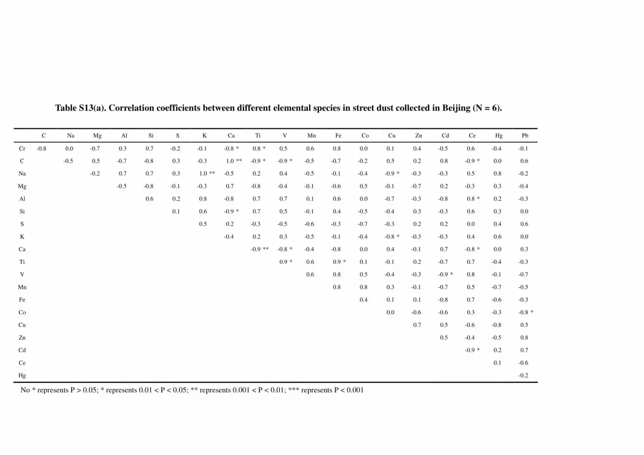
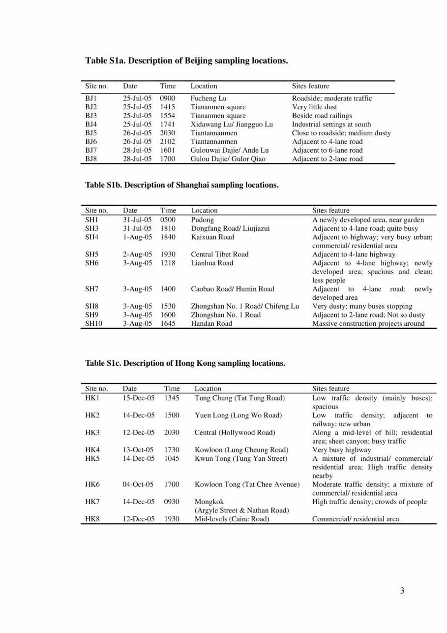
Table S13(a). Correlation coefficients between different elemental species in street dust collected in Beijing (N = 6).
C Na Mg Al Si S K Ca Ti V Mn Fe Co Cu Zn Cd Ce Hg Pb
Cr -0.8 0.0 -0.7 0.3 0.7 -0.2 -0.1 -0.8 * 0.8 * 0.5 0.6 0.8 0.0 0.1 0.4 -0.5 0.6 -0.4 -0.1
C -0.5 0.5 -0.7 -0.8 0.3 -0.3 1.0 ** -0.9 * -0.9 * -0.5 -0.7 -0.2 0.5 0.2 0.8 -0.9 * 0.0 0.6
Na -0.2 0.7 0.7 0.3 1.0 ** -0.5 0.2 0.4 -0.5 -0.1 -0.4 -0.9 * -0.3 -0.3 0.5 0.8 -0.2
Mg -0.5 -0.8 -0.1 -0.3 0.7 -0.8 -0.4 -0.1 -0.6 0.5 -0.1 -0.7 0.2 -0.3 0.3 -0.4
Al 0.6 0.2 0.8 -0.8 0.7 0.7 0.1 0.6 0.0 -0.7 -0.3 -0.8 0.8 * 0.2 -0.3
Si 0.1 0.6 -0.9 * 0.7 0.5 -0.1 0.4 -0.5 -0.4 0.3 -0.3 0.6 0.3 0.0
S 0.5 0.2 -0.3 -0.5 -0.6 -0.3 -0.7 -0.3 0.2 0.2 0.0 0.4 0.6
K -0.4 0.2 0.3 -0.5 -0.1 -0.4 -0.8 * -0.3 -0.3 0.4 0.6 0.0
Ca -0.9 ** -0.8 * -0.4 -0.8 0.0 0.4 -0.1 0.7 -0.8 * 0.0 0.3
Ti 0.9 * 0.6 0.9 * 0.1 -0.1 0.2 -0.7 0.7 -0.4 -0.3
V 0.6 0.8 0.5 -0.4 -0.3 -0.9 * 0.8 -0.1 -0.7
Mn 0.8 0.8 0.3 -0.1 -0.7 0.5 -0.7 -0.5
Fe 0.4 0.1 0.1 -0.8 0.7 -0.6 -0.3
Co 0.0 -0.6 -0.6 0.3 -0.3 -0.8 *
Cu 0.7 0.5 -0.6 -0.8 0.5
Zn 0.5 -0.4 -0.5 0.8
Cd -0.9 * 0.2 0.7
Ce 0.1 -0.6
Hg -0.2
No * represents P > 0.05; * represents 0.01 < P < 0.05; ** represents 0.001 < P < 0.01; *** represents P < 0.001

Table S13(b). Correlation coefficients between different elemental species in street dust collected in Shanghai (N = 8).
C Na Mg Al Si S K Ca Ti V Mn Fe Co Cu Zn Cd Ce Hg Pb
Cr 0.6 -0.6 0.5 -0.4 -0.5 0.8 * -0.5 0.4 0.2 0.4 0.9 ** 0.7 0.8 * 0.7 0.8 * 0.7 * 0.0 0.1 0.9 **
C -0.8 * 0.4 -0.3 -1.0 *** 0.8 * -0.2 0.9 *** -0.5 -0.3 0.6 0.5 0.4 0.2 0.6 0.9 ** 0.6 0.2 0.7 *
Na -0.2 0.8 * 0.7 -0.6 0.6 -0.7 * 0.1 -0.3 -0.7 * -0.4 -0.7 * -0.3 -0.6 -0.9 ** -0.1 0.2 -0.7 *
Mg 0.1 -0.3 0.4 0.3 0.1 0.3 0.0 0.5 0.9 ** 0.3 0.5 0.8 * 0.5 0.4 0.8 * 0.6Al 0.2 -0.2 0.8 * -0.3 -0.1 -0.6 -0.5 -0.1 -0.7 -0.3 -0.3 -0.5 0.3 0.6 -0.4
Si -0.9 ** 0.2 -0.9 ** 0.6 0.3 -0.5 -0.4 -0.4 -0.2 -0.5 -0.8 * -0.6 -0.1 -0.7
S -0.3 0.7 -0.3 0.0 0.6 0.5 0.6 0.4 0.6 0.7 * 0.3 0.1 0.8 *
K -0.2 -0.1 -0.7 -0.5 0.0 -0.8 * -0.5 -0.2 -0.4 0.5 0.7 * -0.4Ca -0.7 * -0.4 0.4 0.2 0.2 0.0 0.3 0.7 0.7 0.0 0.5
Ti 0.8 * 0.3 0.3 0.4 0.4 0.4 0.0 -0.6 0.2 0.1
V 0.4 0.1 0.7 * 0.5 0.3 0.2 -0.8 * -0.4 0.3
Mn 0.7 * 0.8 * 0.7 * 0.9 ** 0.8 * 0.0 0.1 0.9 **
Fe 0.4 0.7 * 1.0 *** 0.7 * 0.4 0.7 0.8 **
Co 0.7 0.7 0.7 * -0.3 -0.2 0.8 *Cu 0.8 * 0.5 -0.1 0.2 0.8 *
Zn 0.8 ** 0.2 0.5 0.9 ***
Cd 0.3 0.2 0.9 ***
Ce 0.6 0.3Hg 0.3
No * represents P > 0.05; * represents 0.01 < P < 0.05; ** represents 0.001 < P < 0.01; *** represents P < 0.001

Table S13(c). Correlation coefficients between different elemental species in street dust collected in Hong Kong (N = 8).
C Na Mg Al Si S K Ca Ti V Mn Fe Co Cu Zn Cd Ce Hg Pb
Cr 0.1 0.0 0.4 -0.3 -0.4 0.2 0.0 0.5 0.4 0.4 0.5 0.7 0.8 * 0.3 0.8 * 0.4 0.1 0.4 0.5
C 0.5 0.7 -0.5 -0.7 * 0.8 ** 0.1 0.6 0.3 -0.6 -0.1 -0.6 -0.2 -0.7 * 0.4 0.9 ** -0.5 -0.1 0.5
Na 0.4 -0.4 -0.6 0.5 -0.3 0.3 -0.1 -0.7 * -0.1 -0.2 0.0 -0.8 * 0.2 0.5 0.0 -0.2 0.7
Mg -0.2 -0.9 ** 0.8 ** 0.0 0.9 ** 0.7 -0.2 0.1 -0.2 0.4 -0.2 0.8 * 0.8 ** 0.2 0.5 0.4
Al 0.5 -0.6 0.6 -0.6 0.2 0.4 0.5 0.1 0.1 0.4 0.0 -0.4 0.7 * 0.3 -0.4 Si -0.9 ** 0.2 -0.9 ** -0.4 0.3 0.0 0.1 -0.3 0.4 -0.7 -0.8 * 0.0 -0.3 -0.6
S -0.3 0.9 ** 0.4 -0.5 -0.2 -0.4 0.1 -0.5 0.4 0.8 * -0.3 0.2 0.4
K -0.4 0.4 0.4 0.8 * -0.1 -0.1 0.0 0.3 0.1 0.3 0.0 0.1
Ca 0.6 -0.2 -0.2 -0.1 0.5 -0.1 0.6 0.8 * -0.1 0.4 0.3 Ti 0.3 0.3 -0.1 0.5 0.2 0.7 * 0.6 0.3 0.4 0.0
V 0.5 0.6 0.4 0.9 ** 0.3 -0.4 0.5 0.3 -0.2
Mn 0.5 0.4 0.2 0.7 0.1 0.5 0.4 0.4
Fe 0.8 * 0.7 0.3 -0.4 0.4 0.5 0.2 Co 0.5 0.7 * 0.2 0.5 0.7 * 0.3 *
Cu 0.1 -0.5 0.5 0.5 -0.4
Zn 0.7 0.4 0.6 0.6
Cd -0.2 0.1 0.5 Ce 0.5 0.0
Hg -0.1
No * represents P > 0.05; * represents 0.01 < P < 0.05; ** represents 0.001 < P < 0.01; *** represents P < 0.001

Table S14. Average concentration (mg kg-1) of Cr in various dusts reported from different countries.
City, country Period Sample typeParticle size, µm
Total Cr Pretreatment Techniquea Ref.
Ottawa, Canada 1993 Road dust 100-250 43 HNO3/HF assisted microwave digestion ICP-MS (27)
Taiwan, China 1995 Road dust <297 130-200High-pressure digestion with HNO3/HClO4
ICP-MS (35)
Yozgat, Turkey 1999 Street dust <30 12-39 Block digestion with aqua regia AAS (36)
Palermo, Italy 2000 Roadway dust 250-500 103 - INAA (37)
125-250 118
63-125 212
40-63 240
<40 203
Luanda, Angola 2002 Street dust <100 26 Heating with HCl/HNO3/H2O ICP-MS (3)
Dhaka, Bangladesh 2003 Street dust <1000 88-136 - XRF (38)
Karak, Jordan 2004 Street dust <2000 4-25 Block digestion with HNO3/HClO3 AAS (39)
Hong Kong, China 2000-2001 Playground dust <250 263HNO3/H2SO4 assisted microwave digestion
AAS (23)
Hong Kong, China 2001-2002 Street dust <86 124 - XRF (12)
Road dust 206 -
aICP-MS inductively-coupled plasma mass spectrometry; AAS atomic absorption spectrometry; INAA instrumental neutron activation analysis;
XRF X-ray fluorescence.
34
References
(3) Baptista, L. F.; Miguel. E. D. Geochemistry and risk assessment of street dust in
Luanda, Angola: A tropical urban environment. Atmos. Environ. 2005, 39, 4501–
4512.
(12) Yeung, Z. L. L.; Kwok, R. C. W.; Yu, K. N. Determination of multi-element profiles
of street dust using energy dispersive X-ray fluorescence. Appl. Rad. Isotopes 2003,
58, 339-346.
(23) Ng, S. L.; Chan, L. S.; Lam, K. C.; Chan, W. K. Heavy metal contents and magnetic
properties of playground dust in Hong Kong. Environ. Monit. Assess. 2003, 89,
221-232.
(27) Rasmussen, P. E.; Subramanian, K. S.; Jessiman, B. J. A multi-element profile of
housedust in relation to exterior dust and soil in the city of Ottawa. Canada. Sci. Tot.
Environ. 2001, 267, 125-140.
(35) Wang, C. F.; Chang, C. Y.; Tsai, S. F. Characteristics of road dust from different
sampling sites in Northern Taiwan. J. Air Waste Man. Assoc. 2005, 55, 1236–1244.
(36) Divrikli, U.; Soylak, M.; Elci, L.; Dogan, M. Trace heavy metal levels in street dust
samples from Yozgat City Center, Turkey. J. Trace Microprobe Techn. 2003, 21,
351–361.
(37) Varrica, D.; Dongarra, G.; Sabatino, G.; Monna, F. Inorganic geochemistry of
roadway dust from the metropolitan area of Palermo, Italy. Environ. Geol. 2003, 44,
222–230.
(38) Ahmed, F.; Ishiga, H. Trace metal concentrations in street dusts of Dhaka city,
Bangladesh. Atmos. Environ. 2006, 40, 3835–3844.
(39) Hasan, T. E.; Batarseh, M.; Omari, H. A.; Ziadat, A.; Alali, Z. A.; Naser, F. A.;
Berdanier, B. W.; Jiries, A. The Distribution of Heavy Metals in Urban Street Dusts
of Karak City, Jordan. Soil Sed. Contamin. 2006, 15, 357–365.

35
Fig. S9. Comparison of street dust compositions for different temporal samplings at CityU.
ዊ�ዊ�ዊ�ዊ�
ዊ�ዊ�ዊ�ዊ�
ዊ�ዊ�ዊ�ዊ�
ዊ�ዊ�ዊ�
ዊ�ዊ�ዊ�
ዊ�ዊ�ዊ�
ዊ�ዊ�ዊ�
ዊ�ዊ�ዊ�
ዊ�ዊ�ዊ�
ዊ�ዊ�ዊ�
ዊ�ዊ� ዊ�ዊ� ዊ�ዊ� ዊ� ዊ�ዊ� ዊ� ዊ�ዊ� ዊ�ዊ� ዊ�ዊ� ዊ�ዊ� ዊ�ዊ� ዊ�ዊ� ዊ�ዊ� ዊ�ዊ� ዊ�ዊ� ዊ�ዊ� ዊ�ዊ�
Elemental species
Con
cent
ratio
n of
the
spec
ies
in d
ust s
ampl
es, l
og10
ዊ�ዊ�ዊ�ዊ�ዊ�ዊ�ዊ�ዊ�ዊ�
ዊ�ዊ�ዊ�ዊ�ዊ�ዊ�ዊ�ዊ�ዊ�
ዊ�ዊ�ዊ�ዊ�ዊ�ዊ�ዊ�ዊ�ዊ�
Fig. S10. Comparison of the variation in street dust composition at CityU using vacuum cleaner and dust pan and brush sampling methods (red: brush/pan; green: vacuum cleaner).
ዊ�ዊ�ዊ�ዊ�
ዊ�ዊ�ዊ�ዊ�
ዊ�ዊ�ዊ�ዊ�
ዊ�ዊ�ዊ�
ዊ�ዊ�ዊ�
ዊ�ዊ�ዊ�
ዊ�ዊ�ዊ�
ዊ�ዊ�ዊ�
ዊ�ዊ�ዊ�
ዊ�ዊ�ዊ�
ዊ�ዊ� ዊ�ዊ� ዊ�ዊ� ዊ� ዊ�ዊ� ዊ� ዊ�ዊ� ዊ�ዊ� ዊ�ዊ� ዊ�ዊ� ዊ�ዊ� ዊ�ዊ� ዊ�ዊ� ዊ�ዊ� ዊ�ዊ� ዊ�ዊ� ዊ�ዊ�
Elemental species
Con
cent
ratio
n of
the
spec
ies
in d
ust s
ampl
es, l
og10
ዊ�ዊ�ዊ�ዊ�ዊ�ዊ�ዊ�ዊ�ዊ�ዊ�ዊ�ዊ�ዊ�ዊ�ዊ�ዊ�ዊ�
ዊ�ዊ�ዊ�ዊ�ዊ�ዊ�ዊ�ዊ�ዊ�ዊ�ዊ�ዊ�ዊ�ዊ�ዊ�ዊ�ዊ�ዊ�ዊ�ዊ�ዊ�ዊ�ዊ�ዊ�ዊ�ዊ�