Embed Size (px)
Citation preview

ARTICLE IN PRESS
Pattern Recognition 43 (2010) 1476–1490
Contents lists available at ScienceDirect
Pattern Recognition
0031-32
doi:10.1
� Corr
E-m
journal homepage: www.elsevier.com/locate/pr
3-D object segmentation using ant colonies
Piergiorgio Cerello a,� , Sorin Christian Cheran a, Stefano Bagnasco a, Roberto Bellotti b,Lourdes Bolanos a,c, Ezio Catanzariti d, Giorgio De Nunzio e, Maria Evelina Fantacci f,Elisa Fiorina g, Gianfranco Gargano b, Gianluca Gemme h, Ernesto Lopez Torres c,Gian Luca Masala i, Cristiana Peroni g, Matteo Santoro j
a I.N.F.N., Sezione di Torino, V. Giuria 1, Torino, 10125 Italyb Dipartimento di Fisica, Universita’ di Bari and I.N.F.N., Sez. di Bari, Italyc CEADEN, Habana, Cubad Dipartimento di Scienze Fisiche, Universita’ di Napoli and I.N.F.N., Sez. di Napoli, Italye Dipartimento di Scienza dei Materiali, Universita’ del Salento and I.N.F.N., Sez. di Lecce, Italyf Dipartimento di Fisica, Universita’ di Pisa and I.N.F.N., Sez. di Pisa, Italyg Dipartimento di Fisica Sperimentale, Universita’ di Torino and I.N.F.N., Sez. di Torino, Italyh I.N.F.N.—Sez. di Genova, Italyi Struttura Dipartimentale di Matematica e Fisica, Universita’ di Sassari and I.N.F.N., Sez. di Cagliari, Italyj Dipartimento di Informatica e Scienze Informatiche, Universita’ di Genova and I.N.F.N., Sez. di Napoli, Italy
a r t i c l e i n f o
Article history:
Received 7 May 2008
Received in revised form
22 August 2009
Accepted 14 October 2009
Keywords:
Artificial life
Ant colony
Image processing
3-D object segmentation
03/$ - see front matter & 2009 Elsevier Ltd. A
016/j.patcog.2009.10.007
esponding author. Tel.: +390116707416; fax
ail address: [email protected] (P. Cerello).
a b s t r a c t
3-D object segmentation is an important and challenging topic in computer vision that could be tackled
with artificial life models.
A Channeler Ant Model (CAM), based on the natural ant capabilities of dealing with 3-D
environments through self-organization and emergent behaviours, is proposed.
Ant colonies, defined in terms of moving, pheromone laying, reproduction, death and deviating
behaviours rules, is able to segment artificially generated objects of different shape, intensity,
background.
The model depends on few parameters and provides an elegant solution for the segmentation of 3-D
structures in noisy environments with unknown range of image intensities: even when there is a partial
overlap between the intensity and noise range, it provides a complete segmentation with negligible
contamination (i.e., fraction of segmented voxels that do not belong to the object). The CAM is already
in use for the automated detection of nodules in lung Computed Tomographies.
& 2009 Elsevier Ltd. All rights reserved.
1. Introduction
Ant Colony Models are computational simulations of antcolonies that use the behaviour rules observed in nature todesign cooperation/competition strategies to be put in place byvirtual agents: the emergence of a global smart behaviour and apurposive self-organization can then be exploited to solve difficultproblems.
Successful applications of Ant Colony Models range from opti-mization techniques [1,2] to swarm robotics [3]. The use of Ant-Colonies in image processing, pattern recognition and objectsegmentation (usually tackled with classical algorithms such asregion growing, active contour and shapes models, watershed tra-nsformations, genetic algorithms, etc.) started in the nineties [4].
ll rights reserved.
: +390116699579.
Many solutions for 2-D image segmentation, thresholding andprocessing were developed but few of them were used in a3-D environment [5–8]. Ant Colony Models are intrinsically 3-D,since all the activities performed by an ant super-organism, likeforging, larvae feeding, nest building, etc. take place in a 3-Denvironment [9].
The approach we propose, called Channeler Ant Model, is astable and elegant solution that requires little tuning (parameter-wise), provides an excellent performance on images with differentdynamic ranges and noise levels and opens a multitude ofpossibilities for further research. The present work was carriedon within the MAGIC-5 Project [10], focused on the developmentof algorithms for the automated detection of anomalies in medicalimages. The Channeler Ant Model discussed here is being adoptedas a tool for the analysis of lung CT scans [11–13], as a way tosegment and remove the background coming from the bronchialand vascular trees in the lungs, which is the biggest source of falsepositive findings in the automated search for nodules.

ARTICLE IN PRESS
P. Cerello et al. / Pattern Recognition 43 (2010) 1476–1490 1477
2. Methods and literature
2.1. Modelling ants
In [1] Bonabeau et al. clearly define the difference betweenmodelling and designing a biological model, i.e., between a trueunderstanding of the ant social behaviour and a mere implemen-tation of some aspects of the natural systems. According to theauthors, when thinking about modelling one tries to uncover andunderstand what happens in an ant colony and how its emergentbehaviour really appears. Every aspect of the model must besupported by biological reasoning. Many aspects of the colonyemerging behaviour like path optimization when forging for food[14,2], raiding patterns formation [15], labour and task division[16], cemetery organization [17], etc. can be modelled.
2.2. Ants in a 3-D environment
Social insects form a decentralized super-organism composedof many cooperative, independent, sensory-motor equippedcomponents that are spread in the environment and respond toexternal stimuli based on local information that can come eitherfrom the environment itself or from other nest mates. Theperception of the colony is the sum of perceptions of all itsmembers, while the colony behaviour is the sum of all theinteractions between the ants and the environment and betweenthemselves. All the activities like forging, cemetery building,larvae feeding and brood sorting take place in the 3-D worldperceived by the individuals [9].
One of the most complex tasks performed by social insects isnest building. Ants were initially thought to be anthropomorphic,1
as if each individual had a 3-D blue print of the global structureembedded into its memory: based on that hypothesis, ants shouldbe able to optimize their decisions and thus the nest complexitywould be the result of the complexity of the insect behaviour. Theobservation of colonies showed that ants are not anthropo-morphic and the amazing nest complexity is the consequence ofthe variety of stimuli to which the individual ants are subjectedand respond. At the beginning of nest building, the behaviour andthe type of response to the stimuli is very simple and unique: anant carrying a pebble that finds a rock on its path will drop its loadand start searching for similar items, so that piles grow bigger,attract more ants and the construction evolves. In a followingphase, the types of stimuli diversify and so does the type ofpossible responses, leading to job diversification and to anincreased nest complexity.
However, even though ants are not anthropomorphic, the nestblue-print does exist: not at the level of each individual but as atemplate found in the environment in the form of physical andchemical heterogeneity that helps organizing the buildingactivities. The process, called stigmergy2 and introduced byGrasse in [18], alongside self-organization helps ants deal with3-D structures.
2.3. Ants in images
Chialvo and Millonas [4] introduced one of the simplest andmost efficient models of trail forming when the ants are notmoving in a closed boundary and are not suppressed by otherbehaviour rules. They compared the trail leaving technique with
1 Having human characteristics.2 Method of communication in emergent systems in which the individual
parts of the system communicate with one another by modifying their local
environment.
the cognitive map patterns from brain science, with the differencethat ants leave their trails in the environment while the‘‘mammalian cognitive maps lie inside the brain’’.
Based on the above paper, Ramos and Almeida [19] developedan extended model where a constant population of ants isdeployed in a digital habitat (i.e., an image) that the insectsperceive and in which they move: they showed that ants are ableto react to different types of digital habitat, achieving in the end aglobal perception of the image as the sum of the local perceptionsof the single colony members.
In the model evolution [20,21] a mechanism that self-regulatesthe population by using the concepts of ageing, death andreproduction in the ant colony is described. The work of Ramosand Almeida is at the root of the model we present in this paper.
Bocchi et al. [6] proposed an image segmentation method thatmakes use of an evolutionary swarm-based algorithm in whichdifferent populations of individuals compete to occupy the 2-Dimage to be analysed. The comparison to other techniquesshowed an improvement in the segmentation of noisy images.Zhuang et al. proposed in [5] a swarm intelligence technique forfeature extraction in image processing, based on Dorigo’s ant
colony system [1] and the perceptual graphs [22] that representthe relationship between adjacent points in the image. The ant
colony system is used to extract just the perceptual graph thatafterwards becomes the basis for a layered model of a machinevision system used for the feature extraction. A method forhierarchical image segmentation, represented by a binary tree, isintroduced in [23], while in [7] Malisia et al. used ant colonyoptimization for image thresholding. Another method for imagesegmentation using behaviour agents that breed and diffuseaccording to the image intensity is found in [8]. George andWolfer [24] presented a swarm intelligence based method for thecounting stacked symmetric objects in digital images.
As seen from the above papers, the literature provides manyexamples of ant colonies implementation in 2-D images based ondifferent algorithms: ant colony systems, perceptual graphs andbinary trees. Unfortunately none of them were scalable or couldbe applied in 3-D imaging with unknown image intensity range.
3. The Channeler Ant Model
The deployment of ant colonies in 3-D images could inprinciple be very effective whenever complex connected struc-tures, with several ramifications of different size and intensity,must be identified and reconstructed, as long as a general modelwith few requirements on parameter tuning is designed andvalidated on images with known properties (different signal tobackground ratio and intensity range).
The development of the Channeler Ant Model (CAM) wastriggered by the idea of using it for the automated search ofsuspect nodules in lung computed tomographies: the CT analysismakes use of the CAM to segment the bronchial and vascular treeand remove it from the CT before the search for nodular structuresin the image with a dedicated filter or with the CAM itself [11,12].
In a way the CAM could be considered an extension of existingmodels [4,19,20], but it also introduces important new features.
Chialvo and Millonas [4] make use of the concept ofprobabilistic directional bias. The probability of a voxel to becomethe ants destination is increased when the ant keeps its directionand such effect is convoluted with the pheromone density in thedefinition of a new ant location. Moreover, the ant population isstatic (there is no evolution driven by birth and death of ants) andthe initial positions are selected randomly. The model describedin [4] was adopted as a starting point by Ramos and Almeida [19],who introduce a correlation between the quantity of pheromone

ARTICLE IN PRESS
P. Cerello et al. / Pattern Recognition 43 (2010) 1476–14901478
that is released and the pixel intensity, a feature that is alsoexploited by the CAM and allows the search for different imagefeatures depending on the choice of the pheromone releasefunction. Ramos et al. [20] improve the model presented in [19]by adding a self-regulation mechanism to the ant population.However, the probability to produce an offspring is related to thenumber of neighbour ants, a feature that does not optimizethe environment exploration: by definition, ants that lead theexploration do not have the highest number of neighbours. Theprobability of dying increases with the lifetime, but unless it doesit rapidly enough it can cause an overcrowding in certain imagevolumes, since no pheromone saturation mechanism that forbidsdestinations is implemented. In the CAM, the energy parameterthat regulates the lifetime of ants changes according to the localproperties of the environment and defines a range within whichants live: above the higher threshold they reproduce, below thelower one they die. With that approach, the forward leading ants
probability of reproducing can be high and the environmentexploration is faster.
Existing models, although extendable to a 3D environment, didnot provide a satisfactory set of rules for the use of ant colonies inimages as complex as lung computed tomography. The Channeler
Ant Model makes use of basic concepts introduced by othermodels [4,19,20] but it changes their implementation in arelevant way:
�
the ants are not set at random positions but start theexploration from an anthill; � the moving rules only depend on the pheromone content atdestination, i.e., there is no directional bias;
� the lifetime is regulated by a double threshold in energy todefine reproduction and death and the number of antsgenerated at each offspring depends on the pheromoneconfiguration in the surroundings;
� the ant colony behaviour is related to the original imagefeatures only via its influence on the pheromone release rules;
� the exploration is guaranteed by a pheromone saturationmechanism, that also provides an intrinsic normalization. Themaximum pheromone content of a voxel is set by a user-defined threshold and does not depend, in the well-exploredvolume, on the original image range of intensity. Moreover,whenever the pheromone content of a voxel is above threshold,it becomes a forbidden destination.
3.1. The colony members
The behaviour of ants, partially derived from [4,19], isdescribed in terms of four modules: the moving rules, thepheromone laying rules, the reproduction/death rules and thedescription of the ant response to anomalies (deviating behaviour).
Ants explore (i.e., ‘‘live in’’) a 3-D spatial environmentdescribed in terms of the properties (position, intensity) ofdiscretized VOlume ELements (voxels) and their life cycle isdefined in terms of atomic time steps, during which ants movefrom one voxel to a neighbour.
So, at time t an ant k is in voxel vi; after one life cycle(time tþ1) it will move to voxel vj. In a 3-D environment, a voxel
has 26 first order neighbours according to Moore’s neighbouringlaw [25].
Two types of individuals live in a colony: the queen and theworker ant.
The queen acts as an observer, performing tasks related to thecolony coordination such as deciding when an ant dies or newants are born.
The workers carry out the nest building (i.e., the objectssegmentation): they move in the habitat and lay pheromoneaccording to its properties and the model rules. Therefore, thefollowing perspectives are possible:
(1)
the Designer’s (Planner)—it envisages the final purpose of thealgorithm, which by means of the ant colony tries to achievethe reconstruction of 3-D objects by defining a set of rules thatdrive the colony evolution: it therefore plans the biggerpicture, specifically by means of choosing the laying rule thatcorrelates the released pheromone amounts to the intrinsicenvironment properties (i.e., the voxel intensities);
(2)
the Queen’s (Observer)—from its point of view the finalpurpose of the algorithm is not interesting nor foreseen; theimportant point is the supervision of the colony evolution.The queen has a global view of the entire habitat but it cannotinterfere, change it in any way nor directly tell the workingunits what they are supposed to do, which direction tochoose, etc. In other words, the queen can see the bigger picturebut is not allowed to set specific aspects or change the colonyrules. The queen implements the pheromone map analysis(see the following sections) and therefore makes use of theglobal knowledge to decide whether voxels are part of thesegmented structure or not.
(3)
the Ant’s (Executor)—it is local, as the single ant only perceivesthe local environment properties at a given time unit andfollows the behaviour rules. The ant has no idea of the globalcolony status, evolution or goal: it focuses on completing itsgiven tasks with no regard to the emergent behaviours thatmight appear in the overall colony.3.2. The ant colony rules
The behaviour of worker ants is defined by a set of rules thatspecify how they move in the environment, how much pher-omone they release before moving to another location, when theyreproduce or die, how they react to anomalies (e.g., when theyreach the environment boundaries): the modelling of each ofthese rules is discussed in the following subsections.
The environment is essentially defined by the voxel imageintensities, which can be thought of as related to the amount ofavailable food for the colony, which should be progressivelyconsumed when the number of visits increases. This mechanism,required to make the colony evolve and explore the environment,is implemented in a complementary way: whenever the limit tothe maximum number of visits (NV ) in a voxel is reached, the voxel
is no more available as a destination.
3.2.1. The moving rules
Randomness is an important factor in self-organization as itcan assure a good balance between following a well establishedpath and the probability of finding new and better paths,triggering the exploration of new regions of the environment.
Like in nature, in the CAM the random component associatedto the way an ant walks is taken into account for the choice of thefuture destination.
However, the choice of the direction for a step must also takeinto account the colony global knowledge of the environment,which is provided by the amount of pheromone already releasedis a given position (sj). The pheromone laying rules are analysedin the following, but the meaning of a pheromone message is thesame as in nature: a large amount of pheromone in a candidatedestination must correspond to a high probability of becomingthe actual destination.

ARTICLE IN PRESS
P. Cerello et al. / Pattern Recognition 43 (2010) 1476–1490 1479
Ants make one step per life cycle: therefore an ant k located invoxel vi at time t must select its destination. The choice is madeaccording to the following rules:
�
only the n¼ 26 first order neighbours are destination candi-dates; � for each voxel neighbour vj, a probability Pij for it to be chosenas destination is computed;
� if an ant is detected in vj, Pij is set to zero; �Cycle Number0 50 100 150 200 250 300 350
<Δph
>
0
200
400
600
800
1000
1200Object: HighwayAverage Pheromone Release
in current cycleglobal
Fig. 1. The average pheromone release as a function of the cycle number: per cycle
(full) and integrated (dashed). The integrated average release becomes more and
more stable as the colony evolves and is therefore suitable for use as a normali-
zation factor.
once a probability of becoming the future destination isassigned to each candidate, one of them is selected by aroulette wheel algorithm.
The probability Pij that a candidate destination is chosen isdefined as follows:
Pijðvi-vjÞ ¼WðsjÞP
n ¼ 1;26WðsnÞð1Þ
where WðsjÞ depends on the amount of pheromone in voxel vj andthe denominator is a normalization factor.
The pheromone-related term WðsjÞ, taken from [4], dependson the osmotro-potaxic sensitivity b (the larger it is, the larger theinfluence of the pheromone trail in deciding the ant’s futuredestination) and on the sensory capacity 1=d (if the pheromoneconcentration is too high, it will determine the decrease of theant’s capability of sensing it):
WðsjÞ ¼ 1þsj
1þd � sj
� �b
ð2Þ
A random number selected in the (0,1] interval determines whichvoxel is actually selected as destination.
3.2.2. Pheromone laying rules
According to the biological laws of ant colonies, before movingto the future destination an ant k deposits in the voxel it is aboutto leave a quantity of pheromone T, defined as [19]
T ¼ ZþDph ð3Þ
where Z is a small quantity of pheromone that an ant would leaveanyway and Dph, the differential quantity of the pheromone, linksthe image properties to the pheromone habitat in which the antslive. Its value is a voxel-intensity dependent function:
Dph ¼CðIÞ ð4Þ
The choice of the depositing rule, made at the Planner level, is veryimportant as it is related to the type of segmentation the ants aregoing to perform. Some possible choices of Dph for an ant thatmoves from voxel vi to vj with intensities IðviÞ and IðvjÞ are shownbelow:
Dph ¼ const � IðviÞ ðRuleIÞ
Dph ¼ const � jIðviÞ � IðvjÞj ðRuleIIÞ
Dph ¼ const �
Pn0
l ¼ 1 IðvlÞ
n0ðRuleIIIÞ
where n0 is the total number of neighbours including the startingvoxel: n0 ¼ nþ1¼ 27 since only first order neighbours areconsidered.
Rule I, in which the ant lays a quantity of pheromone directlyproportional to the intensity of its starting voxel, is used for thesegmentation of objects on a background (e.g., the case of lungcomputed tomographies); Rule II, with a pheromone releaseproportional to the intensity derivative, can be used for borderdetection (e.g., the search for the pleura in lung CTs); Rule III
smooths the effect of the intensity fluctuations and can therefore
be used for segmenting objects in a noisy environment wheneverthe noise fluctuates more than the signal. In the results section,only Rule I is addressed: however, it is important to remark that,just by changing the pheromone deposition rule, it is possible toenhance different image features.
After depositing the pheromone according to the implementedrule, the ant moves to the selected destination voxel.
3.2.3. The life cycle—reproduction and death
Ants, like all the living creatures, live for a finite amount oftime. The life cycle is regulated by a parameter called energy [21],which is assigned at birth with a default value:
e0 ¼ 1þa ð5Þ
The energy variation for ant k must take into account theproperties of the environment, which are defined by the depositedamount of pheromone Dk
ph for the current cycle and by theaverage amount of pheromone per step the colony has depositedsince the beginning of its evolution, used as a normalization factor(/DphS): Fig. 1 shows that the integrated average, used for thenormalization, converges to a constant factor and is far morestable than the average per cycle. Therefore, the energy variationfor ant k is defined as follows:
ektþ1 � e
kt ¼ � a � 1�
Dkph
/DphS
!ð6Þ
The energy range is defined by a lower limit, the death energy eD
and an upper limit, the reproduction energy eR: an ant withenergy ek
t will die whenever ekt oeD and give birth whenever
et 4eR. In that case, the ant energy is reset to the default startingvalue e0. The ant life cycle duration is therefore a function of theratio between the rate of the energy variation (a) and theamplitude of the allowed energy range (eR � eD), all of itmodulated by the properties of the environment.
The number of ants that are generated when a reproductiontakes place (Noffspring) must be related to the local properties of theenvironment, known through the pheromone map generated bythe colony, and take into account the number of free destinationvoxels (nf ).
The local properties of the environment are evaluated bysmoothing the pheromone map at v0 ¼ vðx0; y0; z0Þ and replacing T
with T5, the pheromone release evaluated according to theselected deposition rule when the voxel intensity I is replacedby I5, defined as the average intensity in the voxel’s 125 second

ARTICLE IN PRESS
P. Cerello et al. / Pattern Recognition 43 (2010) 1476–14901480
order neighbours:
I5ðv0Þ ¼1
125
Xxi ;yi ;zi ¼ �2;2
Iðx0þxi; y0þyi; z0þziÞ ð7Þ
For each image, T5;min and T5;max are defined as the smallest andlargest values of T5, respectively. The number of generated antscan be an integer in the ½0;26� interval, since only first orderneighbours are allowed as positions for the generated ants. Theactual number Noffspring is determined assuming that it linearlydepends on T5, with Noffspring ¼ 0ð26Þ corresponding to theminimum (T5;min) and maximum (T5;max) taken by T5, respectively:
Noffspring ¼ 26 �T5ðviÞ � T5;min
T5;max � T5;minð8Þ
In case Noffspring is larger than the number of free neighbours nf , itis set to nf .
3.2.4. The deviating behaviours
Some conditions, not compatible with the above-describedrules, require the definition of the allowed deviating behaviours. Inparticular:
�
when an ant is fully surrounded by fellow mates and anypossible destination voxel is unreachable, the ant is killed; � when an ant reaches the border of the habitat it is killed.3.3. Deploying the model
The Channeler Ant Model, discussed in the previous section,can be easily translated into an algorithm for 3-D imagesegmentation, which hereafter is referred to as the CAM algorithm.It is worth pointing out that the CAM algorithm output is not asegmented image but rather a pheromone map, which can beconsidered an effective preprocessing of the 3-D volume for theactual segmentation, which is discussed in the following and it isactually provided by the analysis of the pheromone map. The CAM
algorithm input–output interface is the following:
Input:
(1) InputImage [A 3-D image, i.e., a collection of N 3-D voxelsvi] (2) Nv [Maximum number of visits for each voxel] (3) NA [(Initial) number of Ants in the colony] (4) vAH [Anthill position, i.e., the voxel where the colony startsbuilding the nest]Output:
(1) PheromoneMap: a 3-D volume that stores the amount ofpheromone released by the ants in each voxel vi of theoriginal image.Some auxiliary data structures are to be defined in order tounderstand the pseudo-code, shown in Fig. 2:
Auxiliary data structures:
(1) NumVisits: an array that stores the number of times an anthas visited a specific voxel.
(2) Ant: a dynamic data structure used to convenientlymanage ants births and deaths in the colony.
Each ant is described by its position AntðviÞ and energyEnergyðAntðviÞÞ.Auxiliary functions:
(1)Fig. 2. The Channeler Ant Model segmentation algorithm Pseudo-code.
EvaluateCandidateDestination ðvi; vjÞ: implements Eqs. (1)
and (2).
DifferentialPheromone ðInputImage; viÞ: implements Eq. (4)on the basis of the selected laying rule of Section 3.2.2.
(2)
(3)
SelectDestination ðPijÞ: selects the actual destination fromthe probability map Pij.
(4)
Move ðAntðviÞ; vjÞ: moves the ant from voxel vi to vj.(5)
UpdateEnergy ðAntðviÞ;DphÞ: implements Eq. (6), requiringthe differential amount of pheromone deposited in thecurrent cycle.
According to the pseudo-code (Fig. 2), the model deployment goesas follows:
�
initially, at t¼ 0, all the voxels are pheromone free: noinformation is available to the ants for their evolution; � an initial ant-hill is chosen in a voxel that belongs to thestructure to be segmented and N0 ¼ 26 ants are released in alldirections (i.e., in all the anthill neighbours) with defaultenergy;
� the ants start moving around in the environment accordingto the above described CAM rules and deposit pheromone;
� the selected rule for depositing pheromone is defined with thegoal of segmenting high intensity regions: Dph ¼ const � IðviÞ,where IðviÞ is the intensity of the voxel on which the ant stands;
� a cycle is finished when all the ants in the population havemade one move;
� after a cycle is completed, the ants energies are updated andcompared to eD and eR;

ARTICLE IN PRESS
Fig. 3. The artificial objects shapes used for the model validation: (a) the toroid, (b) the knot, (c) the highway, (d) the yo-yo, (e) the scale, (f) the 1-Arm bridge, (g) the 2-Arm
bridge.
250
P. Cerello et al. / Pattern Recognition 43 (2010) 1476–1490 1481
�
if a death is triggered then the ant is killed and the number ofmembers in the population updated; �200
if an offspring takes place, the newborn ants are placedrandomly in free neighbouring voxels with default energy andthe colony population is updated;150
� Ythe colony lives and moves until no more ants are alive or untilthe user-predefined number of cycles has been completed;
�X0 50 100 150 200 250
0
50
100
Fig. 4. The 2-D artificial snake used for the model validation.
Table 1Artificial objects properties: the 3-D (2-D) image size in the X, Y, Z directions
(NX ;NY ;NZ ), the number of voxels in the image (NTot) and the number of voxels
belonging to the generated objects (NObject).
once the colony evolution stops the 3-D pheromone map isstored and analysed.
4. Testing the model
4.1. The artificial images
The task of a CAM colony is to provide 3-D pheromone maps ofthe explored volume, to be used as a starting point for thesegmentation of structures. In order to assess the modelperformance, it is important to study its results on a set ofartificially generated 3-D objects with different shape, knownproperties (intensity distribution, background level), in threegroups of increasing complexity:
Object NX NY NZ NTot NObject
�Highway 80 80 80 512000 6800
Class-A set: homogeneous intensity (I¼ I0) objects with zerobackground;
Scale 80 80 80 512000 10824
� Knot 80 80 80 512000 16659Toroid 80 80 80 512000 30332
Yoyo 80 80 80 512000 45116
Class-B set: objects with heterogeneous intensity extractedfrom a Gaussian with mI average and sI standard deviation andzero background;
1-Arm-Bridge 240 80 80 1536 000 56677
� 2-Arm-Bridge 240 80 80 1536 000 57522Snake (2-D) 256 256 1 65536 5292
Class-C set: objects with heterogeneous intensity extracted asfor the Class-B set and a background noise extracted from aGaussian with mnoise average and snoise standard deviation.
The implemented shapes, some of them shown in Fig. 3, wereselected to test the model behaviour in different conditions: thehighway tests that ants truly channel in 3-D; the scale, knot, toroid
and yoyo test the channelling through an object that constantlychanges orientation; the bridges define the colony reaction to thinmulti-branch structures. Moreover, an example of a 2-D object(the snake, shown in Fig. 4) was also selected to demonstrate thatthe model performance in 2-D and 3-D is comparable, as it isexpected according to the model design.
Each object was simulated in three versions, according to thespecifications of classes A;B and C. Table 1 summarizes the sizeand the total number of voxels of the different generated 3-D (2-D)images as well as the number of voxels that are actually part of theartificial object.
4.2. The lung CT images
As quickly addressed in the Introduction, the model wasdeveloped having in mind its use as a module of a lung ComputerAssisted Detection tool, aiming at the identification of nodules inlung computed tomographies. In particular, the CAM is respon-sible of the segmentation of the bronchial and vascular trees inthe lung, so as to be able to remove them from the original imagesand search for nodules in conditions that reduce the number offalse positive candidates.
Although it is beyond the goal of this paper to discuss in detailthe performance on real lung CTs, which requires a carefuldefinition of the radiological truth according to medical protocols,

ARTICLE IN PRESS
P. Cerello et al. / Pattern Recognition 43 (2010) 1476–14901482
an example of pheromone map obtained on a real lung CT will beshown in the following. However, the definition of a metric toquantify the CAM performance in lung CTs is not addressed in thispaper, as it is strongly related to the radiologists’ diagnosis andthe far from obvious definition of a gold standard. A discussion ofthe problem, as well as a very detailed discussion of the CAM (andother algorithms) results on lung CTs as a function of the differenttypes of nodules, is found in [11,12].
4.3. Parameters optimization
The colony evolution is a function of several parameters thatdescribe:
�
the way an ant computes the perceived pheromone quantityfrom a voxel, based on Eq. (2) that contains two parameters:b and d. In [19] the authors discovered the emergence of welldefined networks of trails with b¼ 3:5, d¼ 0:2, the values wedecided to adopt. � the way an ant deposits pheromone in the voxel it is about toleave, set according to Eq. (3). The default quantity ofpheromone that an ant leaves behind (Z), which only certifiesa voxel was visited, must be small; it is defined in such a waythat it is always negligible if compared to pheromone releasesrelevant for the definition of a voxel as segmented:
Z¼ 0:01 ð9Þ
the way the ant energy is updated, according to Eqs. (5) and
�Table 2The properties of the simulated object sets.
Object set Class A Class B/C Class C
Intensity Average Std. dev. Baseline Noise
Set 1 1300 700 200 100 50
Set 2 1600 700 300 100 50
Set 2 1000 700 100 100 25, 50, 75, 100
Set 3 – 700, 1050, 1400 200 100 50
(6): a is a constant that ensures that each ant makes at least afew moves before dying, while the scale factor that determineshow quickly the energy of an ant will increase or decrease,thus deciding how fastly the reproduction and death takeplace, is defined in terms of the local habitat properties.The critical issue is related to the necessity to find asatisfactory equilibrium between two different effects: thecapability to explore new, pheromone free volumes and theminimization of the so-called tunnelling, which causes antsreach unconnected structures. For example, in the case of theToroid-B, the coils of the object are so close to one another that,unless the model parameters are properly tuned, they can bereached by ants that tunnel from a neighbouring coil throughan empty (i.e., low intensity) volume.The maximum number of steps travelled by an ant in apheromone free region is given by
Nsteps ¼ ðeR � eDÞ=a ð10Þ
In order to minimize tunnelling, Nsteps must be small. In thepresent work, the eD, eR and a parameters were set to 1.0, 1.3,0.2, respectively: therefore, in pheromone free areas, no morethan two steps can be travelled.
The limitation to the number of visits a voxel can receive (NV ),introduced in order to make the colony evolve in time along thestructures to be segmented, is not to be considered a modelparameter. Its upper limit defines the speed with whichstructures are segmented, not the capability of ants to segmentthem.
The lower limit must take into account that the number ofvisits a voxel receives is also related to the exploration of itssurroundings: since the definition of the ants future destination isprobability-based, NV must be large enough to allow a statisticallysignificant number of moves to all the neighbours of any visitedlocation.
In other words, NV should be voxel-dependent and its valuemust be inversely related to the pheromone release in that voxel,which in turn depends on the selected laying rule, so that in areas
with small depositions a larger number of visits is allowed,increasing the statistical significance of the results. With NV
ranging in the 40–120 interval, a generic vi to vj step takes placeabout 1.5 (4.5) times in high (low) deposition regions, whichproves to be enough for a satisfactory segmentation. For any givenimage, the pheromone deposition in each voxel can be easilydetermined: assuming it ranges in the whole image from Tmin
to Tmax, the maximum number of visits for a voxel is normalized
as follows:
NV ¼ 40þ80T � Tmax
Tmin � Tmaxð11Þ
In case the pheromone laying rule also depends on the antdestination, T is meant to be the release averaged over all thepossible destinations.
5. Results
Once the model parameters were optimized, the CAM wasdeployed on 3-D artificial objects belonging to classes A;B;C.
The choice of the simulated object properties (intensity andbackground) was driven by the goal of testing the CAMperformance as a function of the object intensity (average andstandard deviation) and background dispersion (i.e., noise).Therefore, different object sets were generated, as summarizedin Table 2.
Each time an ant colony life cycle is completed, a pheromonemap of the original image is available for the analysis, aswell as a map of the number of visits each voxel received:Fig. 5 shows some samples of 2-D slices for the different objectshapes (the full object for the 2-D snake), taken from Set 1/Class-C
objects.The analysis of pheromone maps for the definition of the
segmentation performance will be described in detail later on.
5.1. Colony evolution
The colony population evolution is an interesting marker of thedynamical behaviour during the exploration process: Fig. 6 showsthe evolution for the Set 1/Class C 1-Arm-Bridge and toroid. Theevolution pattern is usually simple, with a triangular-like shape.However, when the anthill is placed along a thin long structure, asit is for the 1-Arm-Bridge, the peak structure appears later, sincethe population growth is prevented until the ants reach thethicker parts of the object.
The number of cycles before the colony extinction and theaverage population are summarized in Table 3 for the differentobject classes of Set 1. The colony life duration depends on theobject complexity and size as well as on the anthill position (forexample, the 1-Arm-Bridge is the last to be completed because theanthill is placed on the thin arm structure). However, an averagetrend can be observed if the same objects of class A, B and C arecompared: the extinction is slightly quicker for objects with

ARTICLE IN PRESS
Original X0 10 20 30 40 50 60 70 80
Y
0
10
20
30
40
50
60
70
80
0
200
400
600
800
1000
1200
Highway
Counts X0 10 20 30 40 50 60 70 80
Y
0
10
20
30
40
50
60
70
80
0
10
20
30
40
50
60
70
Pheromone X0 10 20 30 40 50 60 70 80
Y
0
10
20
30
40
50
60
70
80
0
20
40
60
80
100
120
140
160
310×
Original X
0 10 20 30 40 50 60 70
Y
0
10
20
30
40
50
60
70
0
200
400
600
800
1000
1200
Toroid
Counts X
0 10 20 30 40 50 60 70
Y
0
10
20
30
40
50
60
70
0
10
20
30
40
50
60
70
Pheromone X
0 10 20 30 40 50 60 70
Y
0
10
20
30
40
50
60
70
0
20
40
60
80
100
120
140
160
310×
Original X
0 10 20 30 40 50 60 70 80
Y
0
10
20
30
40
50
60
70
80
0
200
400
600
800
1000
1200
1400
Yoyo
Counts X
0 10 20 30 40 50 60 70 80
Y
0
10
20
30
40
50
60
70
80
0
10
20
30
40
50
60
70
Pheromone X
0 10 20 30 40 50 60 70 80
Y
0
10
20
30
40
50
60
70
80
0
20
40
60
80
100
120
140
160
310×
Original X
0 20 40 60 80 100 120140 160 180 200 220240
Y
0
10
20
30
40
50
60
70
80
0
200
400
600
800
1000
1200
1400
2-Arm-Bridge
Counts X
0 20 40 60 80 100 120 140 160180 200 220 240
Y
0
10
20
30
40
50
60
70
80
0
10
20
30
40
50
60
70
80
Pheromone X
0 20 40 60 80 100120 140 160 180 200220 240
Y
0
10
20
30
40
50
60
70
80
0
50
100
150
200
310×
Original X0 50 100 150 200 250
Y
0
50
100
150
200
250
-400
-200
0
200
400
600
800
1000
1200
Snake (2-D)×
Pheromone X0 50 100 150 200 250
Y
0
50
100
150
200
250
-40
-200
204060
80100
120140160
310
Counts X0 50 100 150 200 250
Y
0
50
100
150
200
250
0
10
20
30
40
50
60
70
Fig. 5. Channeler Ant Model results on some Set 1/Class-C objects: (a) 2-D slice of the original image, (b) 2-D map of voxels visits, (c) 2-D section of the pheromone map.
Row 1: the highway, row 2: toroid, row 3: yoyo, row 4: 2-Arm-Bridge, row 5: 2-D snake.
P. Cerello et al. / Pattern Recognition 43 (2010) 1476–1490 1483

ARTICLE IN PRESS
Cycle Number0 50 100 150 200 250 300 350 400 450 500
Num
ber o
f Ant
s
0
20
40
60
80
100
103
one-Arm-Bridgetoroid
Fig. 6. The colony evolution: the population variation for the segmentation of the
Set 1/Class C 1-Arm-Bridge and toroid as a function of the cycle number. The
standard pattern is triangular-like, with the exception of the 1-Arm-Bridge, where
the location of the anthill along the thin bridge limits the population increase until
the thicker part of the object is reached.
Table 3The number of cycles the colony lives (NCyc) and the average number of ants per
cycle (/NAS) for class A, B and C objects.
Object Class A Class B Class C
NCyc /NAS NCyc /NAS NCyc /NAS
Highway 141 8043 156 7867 162 8863
Scale 206 9365 224 9279 245 10061
Knot 143 20338 148 19394 147 22440
Toroid 139 34242 152 34347 142 40463
Yoyo 241 27050 254 27497 269 29039
1-Arm-Bridge 357 24338 367 25406 418 25683
2-Arm-Bridge 240 37051 251 37870 294 37090
Cycle Number
0 50 100 150 200 250 300 350 400
Num
ber o
f Ant
s
0
20
40
60
80
100
120103
Fig. 7. Number of ants as a function of the cycle number for the segmentation of
the 2-Arm-Bridge starting from different anthill positions. The ant colony evolution
pattern is different, as expected, but the sensitivity and the exploration level are
compatible and show that the CAM performance does not depend on the anthill
location.
P. Cerello et al. / Pattern Recognition 43 (2010) 1476–14901484
uniform intensity (class A), while it takes a little longer (about 10%more cycles) when the intensity is not uniform (class B) andanother 5–10% more when a Gaussian noise is added (class C).Also, the average number of ants in the colony increases by10–15% when adding the noise.
These results are no different than what expected, given themodel rules. The colony average population essentially dependson the pheromone levels, which in turn depend on the imagevoxel intensities: the change from uniform to variable (and lower,on average) intensity causes a slower population increase, andtherefore requires a larger number of cycles to complete thesegmentation.
The addition of a noisy background increases the average lifeof ants, since small pheromone quantities can be released outsidethe object and therefore the ant energy decrease outsidethe object is slower, turning into a larger average number ofliving ants.
The colony evolution is also a function of the anthill location:depending on the local object properties (i.e., the topology in thesurroundings of the anthill), the number of ants in the colonyshows different patterns, as seen in Fig. 7. The peak in the antpopulation is always reached when the thick arm structures arebeing explored. When the anthill is located on (or close to) thethin bridge connecting the two arms, the population reaches aplateau corresponding to the bridge exploration, and increasesagain when the ants reach the arms.
5.2. Object segmentation
As already remarked, the ant colony is deployed and evolvesuntil its extinction, generating a pheromone map which repre-sents the global knowledge of the environment. In order toevaluate the CAM performance with respect to the objectsegmentation, a definition of when voxels are to be consideredas part of the object must be provided. We chose to use aninclusion condition that, applied to the pheromone map, generatesa binary image: whenever a voxel contains more pheromone thana predefined threshold value (Phth), it is classified as segmented.
Therefore, the results are threshold dependent and, inprinciple, shape and set/class dependent.
The following analysis will show that the CAM providesuniform results as well as the possibility of defining a commonthreshold for the pheromone map analysis, which makes itsuitable for the analysis of complex structures with a priori
unknown intensities.In order to quantify the model performance in the segmenta-
tion the following quantities were defined:
�
Sensitivity: S¼NR=NO, i.e., the ratio between the number ofsegmented voxels, evaluated with the pheromone map analy-sis, that actually are part of the object and the number of voxelsin the original object;
� Exploration level: E¼NV=NO, i.e., the ratio between the numberof segmented voxels and the number of voxels in the originalobject;
� Contamination: C ¼NC=NO, i.e., the ratio between the numberof segmented voxels that do not belong to the original objectand the number of voxels in the original object, after thepheromone map analysis.
According to the definitions:
C ¼ ðNV � NRÞ=NO ¼ E� S ð12Þ
S; E and C are function of the threshold value: however, if the mo-del in general enough, they shall not be object shape dependent.
Fig. 8 shows the exploration level (E) and sensitivity (S) for theSet 1/Class A, B and C highway as a function of the selectedpheromone threshold. For class A and B objects, the exploration
level and the sensitivity are coincident, since the pheromone

ARTICLE IN PRESS
Pheromone Threshold
0 20 40 60 80 100 120 140 160 180 200103
E (S
)
0.00.51.01.52.02.53.03.54.04.55.0
Object: highway
Exploration Level (E)
Sensitivity (S), class A/B
Sensitivity (S), class C
Fig. 8. Set 1/Class A, B and C highway: exploration level (E, only for Class C) and
sensitivity (S) as a function of the selected pheromone threshold. The exploration
level for the A, B classes is equal to the sensitivity, since there is no background; for
the C class, it merges with the sensitivity as the pheromone threshold increases.
Table 4
Pheromone threshold Phth and contamination C corresponding to S¼ 0:999 (left
side); pheromone threshold Phth and sensitivity (S) corresponding to C ¼ 0:01
(central part); pheromone threshold Phth and contamination C corresponding to
S¼ 0:99 (right side).
Object S¼ 0:999 C ¼ 0:01 S¼ 0:99
PhTh C PhTh S PhTh C
Highway 16900 0.52 30700 0.996 37200 0.0004
Scale 16700 0.64 31300 0.995 37400 0.0007
Knot 18200 0.41 31500 0.995 36700 0.0011
Toroid 17500 0.42 30100 0.995 36000 0.0007
Yoyo 16300 0.48 30700 0.995 36500 0.0007
1-Arm-Bridge 17100 0.48 31300 0.994 37300 0.0007
2-Arm-Bridge 17900 0.41 30900 0.995 37000 0.0009
Snake 2D 13900 0.34 28300 0.995 35300 0.0013
Contamination0.00 0.02 0.04 0.06 0.08 0.10 0.12 0.14
Sen
sitiv
ity
0.990
0.992
0.994
0.996
0.998
1.000
HighwayScaleKnotToroidYoyo1-Arm-Bridge2-Arm-BridgeSnake
Fig. 9. Set 1/Class C objects: the correlation between the sensitivity and the
contamination (S) shows that the CAM performance is independent of the shape
within a sensitivity range of 0.001.
Contamination0.0 0.2 0.4 0.6 0.8 1.0
Sen
sitiv
ity
0.86
0.88
0.90
0.92
0.94
0.96
0.98
1.00
Highway
Noise Units: 25
Noise Units: 50
Noise Units: 75
Noise Units: 100
Fig. 10. Correlation between the sensitivity and the contamination for the Set 1/
Class C highway (average intensity 700, standard deviation 200) as a function of
the selected pheromone threshold for different noise values.
P. Cerello et al. / Pattern Recognition 43 (2010) 1476–1490 1485
release that takes place when the voxel intensity is zero is so smallthat falls below the smallest threshold value. It is interesting toobserve that adding the noise does not affect the segmentationcapability (the class B, C sensitivity curves are almost the same)while, as expected, it introduces a contamination, caused by thepheromone release in voxels that do not belong to the object.
Given the trend shown in Fig. 8 and the correlation betweenPhth, S and C, three points, defined by the conditions S¼ 0:999,C ¼ 0:01 and S¼ 0:99, were selected as representative of the CAMperformance. Table 4 shows, for the different artificial objects ofSet 1/Class C, the values of Phth and C corresponding at S¼ 0:99 onthe left side, Phth and S at C ¼ 0:01 in the central part and Phth andC at S¼ 0:99 on the right side. The threshold interval between thevalues at C ¼ 0:01 and S¼ 0:99 defines the range corresponding toa satisfactory performance.
Since the sensitivity and contamination are evaluated at eachpheromone threshold value, it is also possible to study theircorrelation with a more general approach. The curves obtained byvarying the pheromone threshold and plotting the sensitivity as afunction of the contamination for the different shapes on the Set
1/Class C objects (Fig. 9) show that the CAM performance isindependent of the shape within a sensitivity range of 0.001 andtherefore the model is general enough to segment differentobjects with similar sensitivity and contamination levels.
It is then essential to study the model behaviour as afunction of the intensity range and the noise level. The correlation
between the sensitivity and the contamination for the Set 2/Class C
highway at different noise levels, shown in Fig. 10, shows—asexpected—that the performance improves as the noise leveldecreases.
The noise level is the most important parameter in discriminat-ing the CAM performance with respect to other algorithms. Sincethe CAM output (i.e., the pheromone map) is analysed with a simplethresholding, a comparison to a simple thresholding on imageintensity provides a measurement of the improvement introducedby the CAM. Fig. 11 shows the results for the two approaches on ahighway with different noise levels: the larger the noise, the betteris the CAM result with respect to the simple thresholding.
That is somehow expected, since in the CAM the channellingfeatures allow the rejection of high intensity voxels that are farfrom the structure being segmented.
In order to compare the CAM results to a more sophisticatedand performing algorithm, a region growing-based (RG) approach[26] was selected, because of its similarities with the CAM inexploring connected structures in a 3-D environment.
Basically, the RG algorithm segments structures starting from aseed point (equivalent to the CAM anthill) and providing inclusion
rules that allow to deterministically decide whether a voxel shouldbe considered as part of the analysed structure or not. Fig. 12 shows

ARTICLE IN PRESS
Sen
sitiv
ity
0.86
0.88
0.90
0.92
0.94
0.96
0.98
1.00
Object: Highway
Thresholding
CAM
Noise: 25 units Sen
sitiv
ity
0.86
0.88
0.90
0.92
0.94
0.96
0.98
1.00
Object: Highway
Thresholding
CAM
Noise: 50 units
Contamination0.0 0.2 0.4 0.6 0.8 1.0
Sen
sitiv
ity
0.86
0.88
0.90
0.92
0.94
0.96
0.98
1.00
Object: Highway
Thresholding
CAM
Noise: 75 units
Contamination0.0 0.2 0.4 0.6 0.8 1.0
Contamination0.0 0.2 0.4 0.6 0.8 1.0
Contamination0.0 0.2 0.4 0.6 0.8 1.0
Sen
sitiv
ity
0.86
0.88
0.90
0.92
0.94
0.96
0.98
1.00
Object: Highway
Thresholding
CAM
Noise: 100 units
Fig. 11. Correlation between the sensitivity and the contamination for the Set 1/Class C highway (average intensity 700, standard deviation 200) at different noise levels, for
the CAM with simple threshold analysis of the pheromone map and a simple thresholding algorithm on the image intensity.
Contamination0.00 0.05 0.10 0.15 0.20 0.25 0.30
Sen
sitiv
ity
0.95
0.96
0.97
0.98
0.99
1.00
Object: Highway
Region GrowingCAM
Noise: 25 units
Contamination0.00 0.05 0.10 0.15 0.20 0.25 0.30
Contamination0.00 0.05 0.10 0.15 0.20 0.25 0.30
Contamination0.00 0.05 0.10 0.15 0.20 0.25 0.30
Object: Highway
Region GrowingCAM
Noise: 50 units
Sen
sitiv
ity
0.95
0.96
0.97
0.98
0.99
1.00
Sen
sitiv
ity
0.95
0.96
0.97
0.98
0.99
1.00
Sen
sitiv
ity
0.95
0.96
0.97
0.98
0.99
1.00
Object: Highway
Region GrowingCAM
Noise: 75 unitsObject: Highway
Region GrowingCAM
Noise: 100 units
Fig. 12. Correlation between the sensitivity and the contamination for the Set 1/Class C highway (average intensity 700, standard deviation 200) at different noise levels, for
the CAM with simple threshold analysis of the pheromone map and a double thresholding (on intensity) Region Growing algorithm.
P. Cerello et al. / Pattern Recognition 43 (2010) 1476–14901486

ARTICLE IN PRESS
Pheromone Threshold
0 50 100 150 200 250 300
103
E (S
)0.0
0.5
1.0
1.5
2.0
2.5
3.0
3.5
4.0
4.5
5.0Object: 2-Arm-Bridge
Max. Intensity: 1400
Max. Intensity: 1050
Max. Intensity: 700
Fig. 14. Exploration level (E) and sensitivity (S) as a function of the selected
pheromone threshold for the Set 3/Class C 2-Arm-Bridge with increasing average
intensity, at constant standard deviation, noise and baseline (i.e., increasing signal
to noise ratio).
P. Cerello et al. / Pattern Recognition 43 (2010) 1476–1490 1487
the comparison for the different noise levels: it is interesting toobserve that, while the performance of the CAM decreases (i.e., thecontamination increases) with the noise, the RG result is verystable. Such a behaviour is strictly related to the fact that the RGdecision is made once and for all while exploring the original image,while the CAM progressively stores information in the pheromonemap which is analysed after the colony extinction. The RG does notsuffer such from a noise increase, since its exploration in a givendirection abruptly stops when just one voxel is below threshold. Onthe other hand, the CAM behaviour is regulated by the ant energy,which allows exploration ranges outside the object that increasewith the noise level. Overall, the CAM performance is better whenthe noise is lower (since the RG anyhow misses a fraction of theobject voxels) while the RG is better at higher noise values.
Such differences can be overcome by introducing a slightlymore sophisticated analysis that takes into account for the CAM(RG) the voxel pheromone amount (intensity) and its average in a3� 3� 3 box around it. The results (Fig. 13) show theperformance of the CAM when only the average pheromonequantity is taken into account and of the RG when both the voxel
intensity and its average with first order neighbours are used forthresholding. The improvement is remarkable, to the extent ofbeing extremely close to a 100% sensitivity for all the noise valuesin a much lower range of contamination values (note that also thex-axis scale differ in Figs. 11–13).
Both the RG and the CAM, therefore, prove to be veryperformant. However, there is an interesting CAM feature thatcould make it preferable to RG. While the RG analysis parameters(i.e., the lower and upper thresholds that are used by the voxel
inclusion rules) operate on the image intensity and thereforemust be tuned whenever the original intensity range changes, theCAM analysis parameter (i.e., the pheromone threshold) does notdepend on the intensity range, as seen in Fig. 14, that shows the
Contamination0.00 0.05 0.10 0.15 0.20
Sen
sitiv
ity
0.990
0.992
0.994
0.996
0.998
1.000
Region GrowingCAM
Noise: 25 units
Contamination0.00 0.05 0.10 0.15 0.20
Sen
sitiv
ity
0.990
0.992
0.994
0.996
0.998
1.000
Region GrowingCAM
Noise: 75 units
Fig. 13. Correlation between the sensitivity and the contamination for the Set 1/Class C h
the CAM with simple threshold analysis of the averaged pheromone map and a double
averaged it is meant that both the pheromone quantities and the image intensities
neighbours).
effect of an increasing signal values at constant noise on theexploration level and sensitivity for the Set 3/Class C 2-Arm-Bridge.The distribution shows that there is no effect on E and S at lowpheromone thresholds, while the plateau with negligiblecontamination and full segmentation progressively extends: inother words, as long as the pheromone threshold is selected forthe worst signal to noise ratio, the segmentation capability is notaffected by increasing the signal range. The CAM behaviour as afunction of the noise at a given average intensity (or, in otherwords, as a function of the average intensity to noise ratio) showsthat, unless the noise levels are very high, it is possible to define a
Contamination0.00 0.05 0.10 0.15 0.20
Contamination0.00 0.05 0.10 0.15 0.20
Sen
sitiv
ity
0.990
0.992
0.994
0.996
0.998
1.000
Region GrowingCAM
Noise: 50 units
Sen
sitiv
ity
0.990
0.992
0.994
0.996
0.998
1.000
Region GrowingCAM
Noise: 100 units
ighway (average intensity 700, standard deviation 200) at different noise levels, for
thresholding (on intensity and averaged intensity) Region Growing algorithm. By
are replaced by the average of a 3� 3� 3 cell (i.e., the voxel and its first order
ARTICLE IN PRESS
Intensity-1000 -500 0 500 1000
Phe
rom
one
0
2000
4000
6000
8000
10000
Intensity300 400 500 600 700 800 900 1000
Cou
nts
0
50
100
150
200
250 Original Image
After Pheromone Analysis
Fig. 15. Pheromone level as a function of the intensity for a lung computed tomography of 512� 512� 313 size (left). Intensity distribution of the set of voxels with
Intensity4300 units and pheromone level o1000 (right).
Original Image Pheromone Map Subtracted Image
Nodule
Fig. 16. An example of the CAM results on a 2-D slice of a lung CT: original image (a), pheromone map (b) and subtracted image (c).
P. Cerello et al. / Pattern Recognition 43 (2010) 1476–14901488
range of pheromone threshold values for which the segmentationis fully satisfactory.
5.3. Lung CT analysis
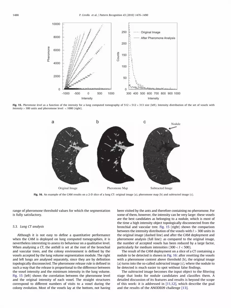
Although it is not easy to define a quantitative performancewhen the CAM is deployed on lung computed tomographies, it isnevertheless interesting to assess its behaviour on a qualitative level.When analysing a CT, the anthill is set at the root of the bronchialand vascular trees, and the colony environment is defined by thevoxels accepted by the lung volume segmentation module. The rightand left lungs are analysed separately, since they are by definitiontopologically disconnected. The pheromone release rule is defined insuch a way that the release is proportional to the difference betweenthe voxel intensity and the minimum intensity in the lung volume.Fig. 15 (left) shows the correlation between the pheromone leveland the original intensity of each voxel. The straight structurescorrespond to different numbers of visits to a voxel during thecolony evolution. Most of the voxels lay at the bottom, not having
been visited by the ants and therefore containing no pheromone. Forsome of them, however, the intensity can be very large: these voxelsare the best candidates as belonging to a nodule, which is most ofthe time a high intensity object topologically disconnected from thebronchial and vascular tree. Fig. 15 (right) shows the comparisonbetween the intensity distribution of the voxels with I4300 units inthe original image (dashed line) and after the CAM deployment andpheromone analysis (full line): as compared to the original image,the number of accepted voxels has been reduced by a large factor,particularly for medium intensities (300o Io500).
The result of the CAM deployment on a slice of a CT containing anodule to be detected is shown in Fig. 16: after resetting the voxelswith a pheromone content above threshold (b), the original image(a) turns into the so-called subtracted image (c), where the nodule tobe detected is much easier to spot without false findings.
The subtracted image becomes the input object to the filteringstage that looks for nodule candidates and classifies them. Adetailed discussion of its features and results is beyond the scopeof this work: it is addressed in [11,12], which describe the goaland the results of the ANODE09 challenge [13].

ARTICLE IN PRESS
P. Cerello et al. / Pattern Recognition 43 (2010) 1476–1490 1489
6. Conclusions and prospects
Artificial ant-colonies have been used in image processing forover a decade, but most of the existing algorithms and modelsdeal with 2-D image segmentation, thresholding or processingproblems. Some approaches treating and using the full capabil-ities of self-organization, trail forging and nest building in an antcolony in 3 dimensions do exist. However, to our knowledge,none of these try to model these capabilities in 3-D imageprocessing.
Since real-ants in nature perform unknown, uncharted objectrecognition every day and they carry on 3-D object constructionin the activity of nest building, artificial ant colonies should beable to do the same.
The Channeler Ants Model describes ants in terms or rules thatdefine their moving capabilities, the pheromone release, the lifecycle (birth, reproduction, death) and the deviating behaviours. Itproves to be suitable for a full segmentation of objects of differentshape, intensity range in a noisy background.
The property of channelling appears as an emergent behaviourof the entire colony, which propagates in the 3-D image, itspopulation being controlled by the energy depletion, until the fullstructure is explored and the colony extinguishes.
The Channeler Ant Model performance was successfullyvalidated on artificial images, without any parameter tuningwhen the image or the environment properties changed.
Moreover, a preliminary analysis of lung computed tomogra-phies shows that the CAM is suitable for use as part of a ComputerAssisted Detection tool for the automated detection of nodules inthe lung.
Acknowledgement
The authors wish to thank the Associazione per lo Sviluppo
Scientifico e Tecnologico del Piemonte for contributing to the workwith a grant.
References
[1] E. Bonabeau, M. Dorigo, G. Theraulz, Swarm Intelligence, from Natural toArtificial Systems, Oxford University Press, Oxford, 1999.
[2] M. Dorigo, V. Maniezzo, A. Colorni, The ant system: optimization by a colonyof cooperating agents, IEEE Transactions on Systems, Man and Cybernetics B26 (1996) 29–41.
[3] /http://www.swarm-bots.org.S.[4] D. Chialvo, M. Millonas, How swarms build cognitive maps, The Biology and
Technology of Intelligent Autonomous Agents 144 (1995) 439–450.
[5] X. Zhuang, N.E. Mastorakis, Image processing with the artificial swarmintelligence, WSEAS Transactions on Computers 4 (2005) 333–341.
[6] L. Bocchi, L. Ballerini, S. Hassler, A new evolutionary algorithm for imagesegmentation, in: EuroGP 2005—EvoWorkshops 2005, Lecture Notes inComputer Science, Springer, Berlin, 2005, pp. 39–43.
[7] A. Malisia, H. Tizhoosh, Image thresholding using ant colony optimization,in: The 3rd Canadian Conference on Computer and Robot Vision, vol. 3, 2006,p. 26.
[8] J. Liu, Y. Tang, Adaptive image segmentation with distributed behaviour-based agents, IEEE Transaction on Pattern Analysis and Machine Intelligence21 (1999) 544–551.
[9] E.O. Wilson, B. Holldobler, The Ants, Harvard University Press, Cambridge,MA, 1990.
[10] R. Bellotti, et al., Distributed medical images analysis on a grid infrastructure,Future Generation Computer Systems 23 (2007) 475–484.
[11] B. Van Ginneken, Automatic NOduleDEtection, in: SPIE2009 Conference, LakeBuena Vista (Orlando Area), FL, USA, 7–12 February 2009.
[12] B. Van Ginneken, et al., Comparing and combining algorithms for computer-aided detection of pulmonary nodules in computed tomography scans: theANODE09 study, Medical Image Analysis, submitted for publication.
[13] /http://anode09.isi.uu.nl/S.[14] J.-L. Deneubourg, S. Aron, S. Goss, J.-M. Pasteels, The self-organizing
exploratory pattern of the argentine ant, Journal of Insect Behavior 3(1990) 159–168.
[15] J.-L. Deneubourg, N.R. Franks, S. Goss, J.-M. Pasteels, The blind leading theblind: modelling chemically mediated army ant raid patterns, Journal ofInsect Behavior 2 (1989) 719–725.
[16] E. Bonabeau, G. Theraulz, J.-L. Deneubourg, Quantitative study of the fixedthreshold model for the regulation of division of labor in insect societies,Proceedings of the Royal Society London B 323 (1996) 1565–1569.
[17] J.-L. Deneubourg, S. Goss, A. Sendova-Franks, C. Detrain, L. Chretien, Thedynamics of collective sorting: robot-like ant and ant-like robot, ProceedingsFirst Conference on Simulation of Adaptive Behavior, vol. 1, MIT Press,Cambridge, MA, 1991, pp. 356–365.
[18] P.-P. Grasse, Termitologia, Tome II. Fondation des Societes. Construction,Masson, Paris, 1959.
[19] V. Ramos, F. Almeida, Artificial ant colonies in digital image habitats—a massbehaviour effect study on pattern recognition, in: Proceedings of ANTS2000—2nd International Workshop on Ant Algorithms (From Ant Colonies toArtificial Ants), Belgium, 2000, pp. 39–43.
[20] V. Ramos, C. Fernandes, A.C. Rosa, Self-regulated artificial ant colonies ondigital image habitats, in: Proceedings of the ICANN’05: 15th InternationalConference, Lecture Notes in Computer Science, vol. 3696, Springer, Berlin,2005, pp. 311–316.
[21] V. Ramos, C. Fernandes, A.C. Rosa, Varying the population size of artificialforging swarms on time varying landscapes, in: Proceedings of the ICANN’05:15th International Conference, Lecture Notes in Computer Science, vol. 3696,Springer, Berlin, 2005, pp. 311–316.
[22] F. Meyer, Skeletons and perceptual graphs, Signal Processing 16 (1989)335–363.
[23] P. Khajehpour, C. Lucas, B. Araabi, Hierarchical image segmentation using antcolony and chemical computing approach, in: Advances in Natural Computa-tion, vol. 3611, Springer, Berlin, 2005, p. 1250.
[24] C. George, J. Wolfer, A swarm intelligence approach to counting stackedsymmetric objects, in: Artificial Intelligence and Applications, Acta Press,Austria, 2006.
[25] E.F. Moore, Gedanken experiments on sequential machines, AutomataStudies, 1956.
[26] R. Bellotti, et al., A CAD system for nodule detection in low-dose lung CTsbased on region growing and a new active contour model, Medical Physics 34(12) (2007) 4901–4910.
About the Author—PIERGIORGIO CERELLO graduated in Physics in 1989 at the Univ
ersity of Torino. After 2 years spent at CERN, he started a Ph.D. in Physics, completed in1995 at the University of Torino. He is a member of the CERN/ALICE Project, with contributions in the area of interfaces to Grid Services and software for the silicon driftdetectors. Since 2003 he is Project Coordinator of MAGIC-5, focused on the developments of software for the automated detection of anomalies in medical images, to beused in a distributed environment.About the Author—SORIN CRISTIAN CHERAN has graduated in 2003 in Computer Science Faculty from Politehnica University of Bucharest. Holds a Ph.D. in Computer Scienceobtained in 2007 from the Universita degli Studi di Torino. Presently he is working for Hewlett Packard EMEA as a High Performance Computing Engineer and Solution Architect.
About the Author—STEFANO BAGNASCO graduated in Physics in 1996 from University of Torino, Italy and, after one year at Fermilab, obtained his Ph.D. in 2001 fromUniversity of Genova, Italy, working on the BaBar experiment. He is currently working in the context of the ALICE experiment at CERN and of the European Grid initiativeEGEE. He has also worked on the development of an interface to Grid Service of a mammogram analysis station.
About the Author—ROBERTO BELLOTTI graduated in Physics at the University of Bari in 1988. He is presently Associate Professor of Experimental Physics at the University of Bari, Italy.His research takes place in the areas of Medical Physics, where he took part in the development of CAD systems for the breast and lung cancer detection, and Experimental Physics.
About the Author—LOURDES BOLANOS is a Researcher at the CEADEN, Habana, Cuba. She spent one year as University of Torino fellow at INFN, Torino and worked on themanuscript review as well as on the use of the Channeler Ant Model for the analysis of lung computed tomographies.

ARTICLE IN PRESS
P. Cerello et al. / Pattern Recognition 43 (2010) 1476–14901490
About the Author—EZIO CATANZARITI is Associate Professor of Computer Science at the Faculty of Sciences of Universit�a di Napoli Federico II. His research interests spanthe fields of computer vision, computational models of brain, remote sensing and pattern recognition with special focusing on medical image analysis, automated diagnosisand recognition and control of object-directed actions.
About the Author—GIORGIO DE NUNZIO received the Master’s degree in Physics from the University of Salento (Lecce, Italy) (1991), and a Ph.D. from the University ofMontpellier II (1995). Since 2001 he is with the University of Salento, where he is Researcher in Applied Physics. His research interests focus on physics, informatics, andimage processing, applied to medicine and cultural heritage.
About the Author—MARIA EVELINA FANTACCI is a Researcher of Medical Physics at the University of Pisa. Main interests in the development of algorithms for theComputer Assisted Detection of signatures in medical images.
About the Author—ELISA FIORINA graduated in Physics at the University of Torino in 2007 with a thesis on the Channeler Ant Model performance on artificial objects.
About the Author—GIANFRANCO GARGANO graduated in Physics in 2001 and got a Ph.D. in Physics in 2006 at the University of Bari. Since 2003 his research activityfocuses on the development of Computer Aided Detection Systems lung nodules in CT scans.
About the Author—GIANLUCA GEMME got his Master degree in Physics in 1989, at the University of Genoa. In 1993 he got a permanent position as Technical Scientist atINFN and since 2003 he has been Senior Researcher at INFN. Since 2005 he joined the research program Magic-5 (Medical Application on a Grid Infrastructure Connection)of INFN.
About the Author—ERNESTO LOPEZ TORRES graduated in Nuclear Physics at the Instituto Superior de Ciencias y Tecnologıa Nucleares, Cuba, in 1991. He is presentlyworking on the Monte Carlo Simulation and particle transport in the ALICE experiment at CERN and on the use of Ant Colonies for the object segmentation on artificialobjects and medical images.
About the Author—GIOVANNI LUCA MASALA graduated in Electronic Engineering in 2002; he completed a Ph.D. in Physics in 2006. His research activities are in the fieldof Physics Applied to Medicine and Pattern Recognition.
About the Author—CRISTIANA PERONI is a Professor of Medical Physics at the University of Torino. Research activity in medical physics, with main interests in thedevelopment of devices for the dosimetry and monitoring of therapeutical beams of photons, electrons and hadrons in collaboration with research centers and withindustry.
About the Author—MATTEO SANTORO obtained a Ph.D. in Computer Science and a Degree in Physics from the University of Naples (Italy). Currently, he is a post-doc atDISI, University of Genova (Italy), where his research work aims at building knowledge discovery and decision support systems based on the multi-modal integration ofbiomedical information. His main interests are: statistical inference, machine learning and inverse problems for biomedical data analysis.