Electronic copy available at: http://ssrn.com/abstract=2217772

University of Oslo

University of Oslo Faculty of Law Legal Studies Research Paper Series

No. 2013-10

Edward Anderson, University of East Anglia

Malcolm Langford, University of Oslo

A Distorted Metric: The MDGs and State Capacity

Electronic copy available at: http://ssrn.com/abstract=2217772Electronic copy available at: http://ssrn.com/abstract=2217772

1

A  Distorted  Metric:  The  MDGs  and  State  Capacity  

Edward Anderson * and Malcolm Langford**

Abstract. The Millennium Development Goals (MDGs) have been commonly understood as national targets. This interpretation has fostered the critique that the framework favours complacent middle-income countries, discriminates against low-income countries, provides a poor national planning tool and generally fails to conform to the more nuanced obligations of states under international human rights law, such as the duty to use the maximum available resources to realise socio-economic rights. The result is that the current MDGs framework (and its likely successor in 2015) may be an unreliable and misleading indicator of progress when used as a cluster of national benchmarks. This paper tests this potential bias in the framework by measuring performance on two MDG targets, water and sanitation, from the perspective of state capacity. A number of proxy indicators are used to capture the relevant resources: GDP per capita; the ratio of ‘disposable national income’ (DNI) to GDP; total population; land area; urbanisation and the dependency ratio. The relationship between this capacity and actual progress on access to water and sanitation is measured for both levels and changes in resources between 1990 and 2010. The resource-adjusted performance of states is then ranked according to two alternative methods and compared with the ranking generated by the standard MDG metric. The paper concludes by arguing that the post-2015 agenda needs to address the distortion and disincentives created by the MDG framework and suggests a number of practical means of doing so.

Comments on the paper welcome

Lecturer, School of International Development, University of East Anglia. Email: edward.Anderson@uea.ac.uk ** Research Fellow, Norwegian Centre for Human Rights, University of Oslo. Email: malcolm.langford@nchr.uio.no Acknowledgment: The initial research findings were first presented at the Third Annual Meeting of Human Rights Metrics, in collaboration with the Center for Economic and Social Rights,, Madrid, 22-23 March 2012. We would like to sincerely thank participants for their feedback.

Electronic copy available at: http://ssrn.com/abstract=2217772Electronic copy available at: http://ssrn.com/abstract=2217772

2

1.  Introduction  

Within a short period of time, the Millennium Development Goals (MDGs) were understood

and established as national benchmarks. Whether it was the halving income poverty, reducing

maternal mortality by two-thirds, or ensuring full access in universal primary education, each

country was given the same target. With the assistance of UNDP, States soon began

producing national reports on progress which were collated into comparative reports by the

UN, World Bank and others. They indicated which countries were ‘on-track’ or ‘off-track’.

This methodological nationalism was reinforced by efforts to use the targets as national

planning tool. A model of MDG-based planning and costing with 2015 set as the end date was

encouraged and piloted (see for a range of discussion Atkinson, 2006; Bourguignon et al.,

2008; Chakravarty and Majumber, 2008).

The approach has been subject to critique. One of the architects of the MDGs argued that it

was ‘denial’ of their very intention: “The quantitative targets were set in line with global

trends, not on the basis of historical trends for any particular region or specific country”

(Vandemoortele, 2007: 1).1 Easterly (2009) complains that Africa was set up for failure: the

goals had the “unfortunate effect” of making the “successes” of this region “look like

failures”. The problem with the MDGs metric becomes clear once the magnitude of a

proportional reduction is compared across countries. The baseline proportion of people living

in poverty in South Africa was 24.3 per cent: for Tanzania it was 72.6 per cent.2 In other

words, South Africa was required to reach a quarter of its population; Tanzania three-quarters.

Moreover, the baseline was set in the year 1990 (with most baseline data coming from

surveys in the early 1990s). This favoured countries which made significant progress before

the new millennium commenced. It led to the rather odd situation where upon the adoption of

the MDGs, China was announce that it had already met the MDG income poverty target, in

1999 (Pogge, 2004). It was not alone in trumpeting its rapid achievements. A number of other

middle and high-income States soon announced they reached the target or were ‘on-track’

(OHCHR, 2010).

1 See also Vandemoortele (2011) for an expanded argument. 2 See data at: http://www.cgdev.org/section/topics/poverty/mdg_scorecards

3

Tabatabai (2007) has responded to this criticism by noting that conflating the basis of

measurement with the intention of the MDGs would be rather meaningless: meeting historical

trends would make a weak case for adopting the framework in the first place. Rather, the

function of the MDGs was to “accelerate trends” which would “encourage weak performers to

lift themselves up to the average level”. However, Tabatabai conceded that it would be a

mistake to use the MDGs yardstick to classify some countries as failures, as such an

assessment can only be made by assessing the circumstances for the country. Tabatai also

notes that some countries had adopted more ambitious targets at the national level, in order to

compensate for “a conservative interpretation of the MDGs”. 3 However, Sumner and

Melamed (2010) find that only 24 states had adopted some form of ‘MDG-Plus’ model

although the extent of these adaptions varies considerably – and to that could be added the

reporting on them.

The MDGs thus contained an internal contradiction. The discourse and intentions were

forward-looking, as Tabatabai rightly states. But once the targets were applied as a singular

template to all counties the monitoring framework there was a risk that they would become

biased towards past achievements: rewarding previous performance.

The MDGs monitoring framework also faced criticism from the perspective of human rights.

The targets over-shadowed the more nuanced and national-sensitive human rights framework

(Amnesty, 2010; Langford, 2010; UN-OHCHR, 2008). 4 For instance, widely ratified

international treaties such as the International Covenant on Economic, Social and Cultural

Rights (ICESCR) and the Convention on the Rights of the Child instead require states to use

their “maximum available resources” to “progressively achieve” economic, social and cultural

rights.5 Thus the pace of expected achievement is dependent on capacity. This is not to

3 See for example, UNDP, MDG-Plus: a case study of Thailand, (New York: UNDP, undated). Similarly, in Latin America and the Caribbean, the region went beyond the MDG target of universal primary education to set a secondary education target of 75 per cent of children by 2010. See Inter-American Development Bank, The Millennium Development Goals in Latin America and the Caribbean: Progress, Priorities and IDB Support for Their Implementation (Washington: IADB, 2005), p. 24. 4 Thus, the human rights critique was not simply about whether the global goals were under-ambitious or not (cf. Alston, 2005; Pogge, 2004) or excluded key human rights or issues (Antrobus, 2003; UNIFEM, 2004), but about whether they reflected the more qualitative and heavily-negotiated gradation in international law. 5 Article 2(1) of ICESCR reads: “Each State Party to the present Covenant undertakes to take steps, individually and through international assistance and co-operation, especially economic and technical, to the maximum of its available resources, with a view to achieving progressively the full realization of the rights recognized in the present Covenant by all appropriate means, including particularly the adoption of legislative measures.” Article 4 of the Convention on the Rights of the Child reads: “States Parties shall undertake all appropriate legislative,

4

overshadow the fact that these treaties have been interpreted to contain a minimal standard of

achievement which might correspond to some of the MDGs (Alston, 2005). In General

Comment No. 3, the UN Committee on Economic, Social and Cultural Rights (CESCR)

stated: “a State party in which any significant number of individuals is deprived of essential

foodstuffs, of essential primary health care, of basic shelter and housing, or of the most basic

forms of education is, prima facie, failing to discharge its obligations under the Covenant”. 6

However, the Committee noted that poorer or fragile countries could plead insufficient

resources if they could establish that “every effort has been made”.7 Further, and more

importantly, countries with greater capacity were required to make brisker progress in terms

of achieving satisfactory level of the rights for all.8

Given that the national-based approach to monitoring remains dominant, it is important to

examine to what extent does the MDGs metric distort the picture of progress.

In this paper, we set out an approach to assessing state performance with regard to MDG

outcomes which takes into account differences in state capacity. This issue has been at the

core of the concerns over the MDGs framework and also fits with the duty of states to use

their maximum available resources to realise the relevant rights under international treaty law.

We apply this approach to access to water and sanitation, which feature both as MDG targets

and as universally accepted human rights. In Millennium Development Goal 7, states

committed to halve the proportion of those without access to an improved source water and

sanitation by 2015. Since 1977, water and sanitation have been recognised as human rights in

a range of international instruments9 and authoritatively so by the UN General Assembly and

UN Human Rights Council in 2010.10 The CESCR has affirmed that these rights attract the

administrative, and other measures for the implementation of the rights recognized in the present Convention. With regard to economic, social and cultural rights, States Parties shall undertake such measures to the maximum extent of their available resources and, where needed, within the framework of international co-operation.” 6 General Comment 3, The nature of States parties' obligations, (Fifth session, 1990), U.N. Doc. E/1991/23, annex III at 86 (1991), para. 10. For legal commentary, see Alston (1992); Langford and King (2008). 7 “In order for a State party to be able to attribute its failure to meet at least its minimum core obligations to a lack of available resources it must demonstrate that every effort has been made to use all resources that are at its disposition in an effort to satisfy, as a matter of priority, those minimum obligations.” Ibid. para. 3. 8 The Committee stated that progressive realisation “imposes an obligation to move as expeditiously and effectively as possible”. Ibid. para. 9. 9 For an overview, see Langford and Russell (2013). 10 In July 2010, the UN General Assembly recognised “the right to safe and clean drinking water and sanitation as a human right that is essential for the full enjoyment of life and all human rights”. U.N. General Assembly, The human right to water and sanitation (Sixty-fourth session, 2010) U.N. Doc A/64/L.63/Rev.1, para. 1.

5

duty of progressive realisation within maximum available resources in accordance with

Article 2(1) of the ICESCR.11 By focusing on water and sanitation only, we are able to go

beyond the use of GDP as a single indicator of state capacity and build a more fine-grained set

of indicators that reflect the relevant state capacity for realising particular targets.12

The paper proceeds as follows. In section 2 we set out our approach to assessing state

performance, taking state capacity into account, and present the indicators we use to measure

state capacity in relation to access to water and sanitation. In section 3 we apply this approach

to comparisons of performance across countries, using data for 2010 or 2005, and compare

the rankings generated by our approach with those generated by the SERF Index.13 In section

4 we apply our approach to comparisons of trends in performance between 1990 and 2010 (or

2005, and compare the rankings generated by our approach with the rankings generated by a

traditional MDG metric. In section 6, we conclude by arguing that the post-2015 agenda

needs to address the distortion and disincentives created by the MDG framework and suggest

a number of practical means of doing so.

However, a high number of States abstained from voting for this resolution: 122 voted in favour to none against, with 41 abstentions (including a number of EU member states). The majority of abstaining States noted that their vote was based on procedural grounds: the matter was also being handled by the UN Human Rights Council. Three months later in September 2010, the UN Human Rights Council affirmed the recognition of the right to water and sanitation, and its legal etymology, without the need to hold a vote: “(The Council) Affirms that the human right to safe drinking water and sanitation is derived from the right to an adequate standard of living and inextricably related to the right to the highest attainable standard of physical and mental health, as well as the right to life and human dignity.” U.N. Human Rights Council, Human rights and access to safe drinking water and sanitation (Fifteenth session, 2010) U.N. Doc. A/HRC/15/L.14. 11 See Committee on Economic, Social and Cultural Rights, General Comment 15, The right to water (Twenty-ninth session, 2002), U.N. Doc. E/C.12/2002/11 (2003); UN Committee on Economic, Social and Cultural Rights, Statement on the Right to Sanitation, (Forty-fifth session, 2010), UN Doc. E/C.12/2010/ 1. 12 The paper builds on earlier work in Dugard, Langford and Anderson (2013) where we compared performance of municipalities across South Africa based on their respective capacities. 13 See Randolph, Fukuda-Parr and Lawson-Remer (2010) for a discussion of the SERF Index.

6

2.  Assessing  water  and  sanitation  performance:  methodology  

2.1   Overall  approach  

Our aim is to assess the performance of national governments in raising access to water and

sanitation, taking into account their ‘capacity’: i.e., their ability to raise access through policy

interventions and spending programmes financed by internal and/or external resources. We

assume that access is determined partly by government capacity, but also by government

performance, defined broadly to cover both the degree of priority attached by the government

to water and sanitation, relative to other goals, and the efficiency with which the government

makes use of resources.

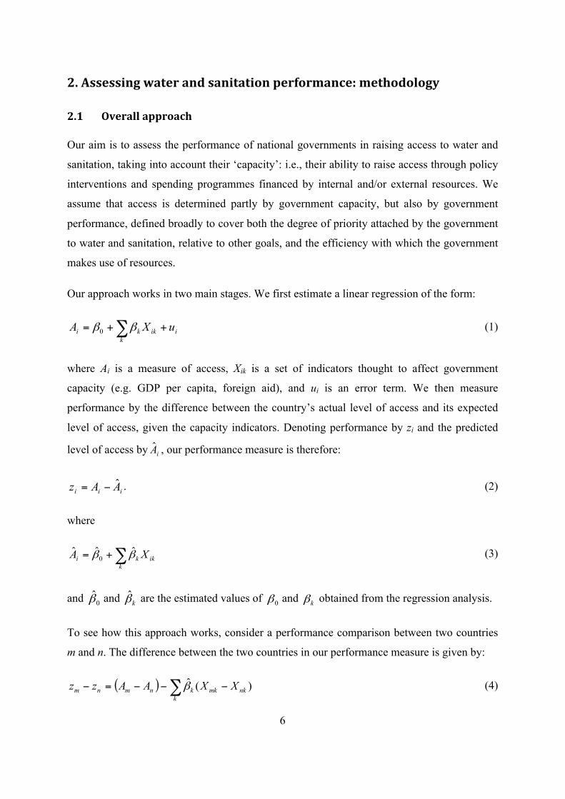
Our approach works in two main stages. We first estimate a linear regression of the form:

ik

ikki uXA ++= ∑ββ0 (1)

where Ai is a measure of access, Xik is a set of indicators thought to affect government

capacity (e.g. GDP per capita, foreign aid), and ui is an error term. We then measure

performance by the difference between the country’s actual level of access and its expected

level of access, given the capacity indicators. Denoting performance by zi and the predicted

level of access by iA , our performance measure is therefore:

iii AAz ˆ−= . (2)

where

∑+=k

ikki XA ββ ˆˆˆ0 (3)

and 0β and kβ are the estimated values of 0β and kβ obtained from the regression analysis.

To see how this approach works, consider a performance comparison between two countries

m and n. The difference between the two countries in our performance measure is given by:

( ) ∑ −−−=−k

nkmkknmnm XXAAzz )(β (4)

7

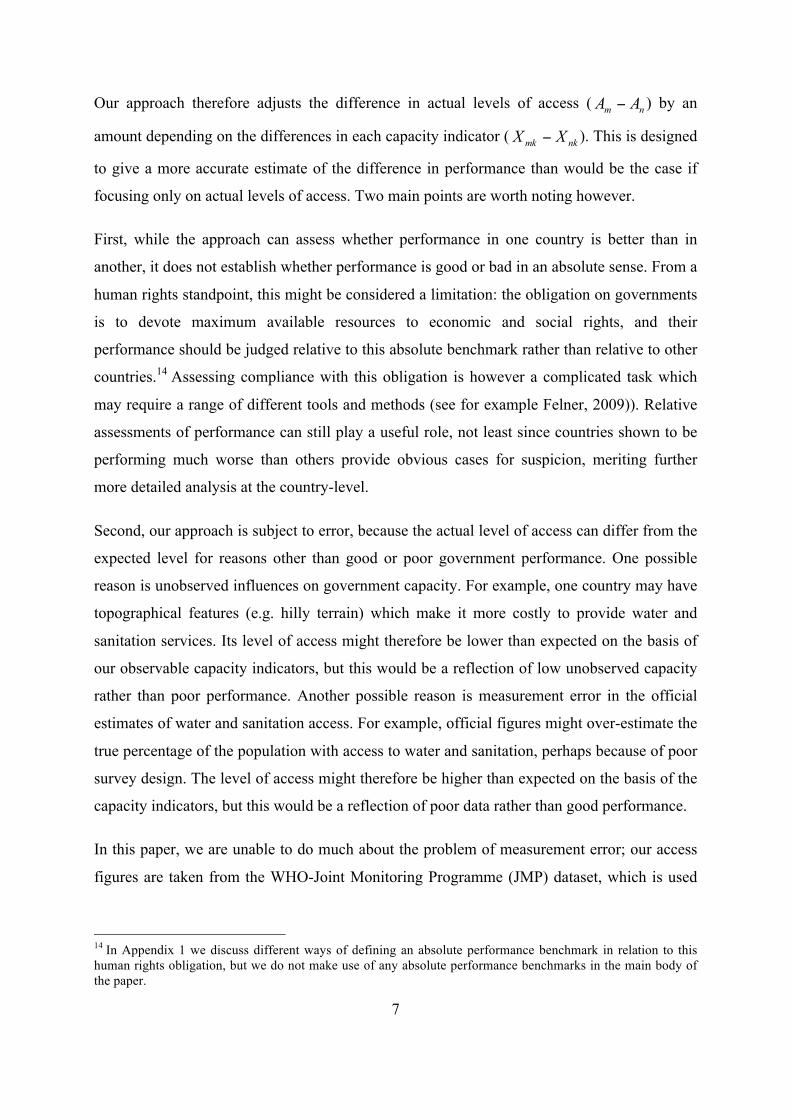
Our approach therefore adjusts the difference in actual levels of access ( nm AA − ) by an

amount depending on the differences in each capacity indicator ( nkmk XX − ). This is designed

to give a more accurate estimate of the difference in performance than would be the case if

focusing only on actual levels of access. Two main points are worth noting however.

First, while the approach can assess whether performance in one country is better than in

another, it does not establish whether performance is good or bad in an absolute sense. From a

human rights standpoint, this might be considered a limitation: the obligation on governments

is to devote maximum available resources to economic and social rights, and their

performance should be judged relative to this absolute benchmark rather than relative to other

countries.14 Assessing compliance with this obligation is however a complicated task which

may require a range of different tools and methods (see for example Felner, 2009)). Relative

assessments of performance can still play a useful role, not least since countries shown to be

performing much worse than others provide obvious cases for suspicion, meriting further

more detailed analysis at the country-level.

Second, our approach is subject to error, because the actual level of access can differ from the

expected level for reasons other than good or poor government performance. One possible

reason is unobserved influences on government capacity. For example, one country may have

topographical features (e.g. hilly terrain) which make it more costly to provide water and

sanitation services. Its level of access might therefore be lower than expected on the basis of

our observable capacity indicators, but this would be a reflection of low unobserved capacity

rather than poor performance. Another possible reason is measurement error in the official

estimates of water and sanitation access. For example, official figures might over-estimate the

true percentage of the population with access to water and sanitation, perhaps because of poor

survey design. The level of access might therefore be higher than expected on the basis of the

capacity indicators, but this would be a reflection of poor data rather than good performance.

In this paper, we are unable to do much about the problem of measurement error; our access

figures are taken from the WHO-Joint Monitoring Programme (JMP) dataset, which is used

14 In Appendix 1 we discuss different ways of defining an absolute performance benchmark in relation to this human rights obligation, but we do not make use of any absolute performance benchmarks in the main body of the paper.

8

for current MDG monitoring and is arguably the most reliable source available – although it

faces some clear construct and statistical validity limitations.15 We do however seek to limit

errors caused by unobserved influences on government capacity, by including a larger set of

capacity indicators is than has been the case in previous work. This is discussed further in the

next sub-section.

2.2   Data  and  indicators  

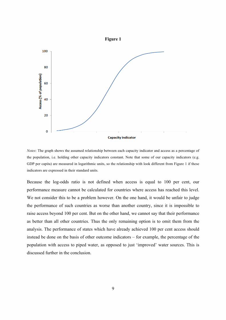
In implementing our approach, we measure access by the ‘log-odds ratio’, i.e. the ratio of the

percentage of the population with access to the percentage of the population without access,

expressed in logarithmic units. This tended to yield the best fit when estimating equation (1);

it implies that the relationship between access as a percentage of the population and any one

capacity indicator takes the form of an S-shaped curve (see Figure 1). This shape is consistent

with the argument that it becomes increasingly difficult to raise access to water and sanitation

as the percentage with access approaches 100, since this requires providing services to areas

with less favourable geographical and economic conditions and therefore higher costs (e.g.

Krause 2009). Countries with moderate historical levels of access should therefore find it

easier to raise access by a certain amount (in percentage points). It is also consistent with the

finding that countries with historically low levels find it harder to get moving (Anand 2006),

suggesting that economies of scale might be a challenge for countries at very low levels of

access.16 It is also possible that the flattening out effect as access approaches 100 per cent may

have something to do with political will – not providing access to an ethnic minority like the

Roma for example; we need to be careful that lack of political will is not turned into a

capacity constraint.

15 Former UN officials have noted that the definition for access to water is too permissive and sanitation too strict (Bartram, 2008: 283) while others have demonstrated that the water supply may be irregular or not potable (Mboup, 2005), not affordable (Smets, 2009) or culturally unacceptable (Singh, 2013). 16 Anand does not offer a hypothesis as to why this might be the case. He states: “There is strong evidence to suggest that legacy in terms of the starting point matters and as such there is a bigger mountain to climb for those countries which are starting with a lower base.” (p. 19). However, he also notes that a significant number of countries are able to break with that legacy suggesting it is not a hard constraint. However, one possible reason might be economies of scale. In countries with dated infrastructure and high population growth, significant infrastructural and water management investment is needed to reach the majority of the population. It is not a case of just extending networks or water supply projects.

9

Figure 1

Notes: The graph shows the assumed relationship between each capacity indicator and access as a percentage of

the population, i.e. holding other capacity indicators constant. Note that some of our capacity indicators (e.g.

GDP per capita) are measured in logarithmic units, so the relationship with look different from Figure 1 if these

indicators are expressed in their standard units.

Because the log-odds ratio is not defined when access is equal to 100 per cent, our

performance measure cannot be calculated for countries where access has reached this level.

We not consider this to be a problem however. On the one hand, it would be unfair to judge

the performance of such countries as worse than another country, since it is impossible to

raise access beyond 100 per cent. But on the other hand, we cannot say that their performance

as better than all other countries. Thus the only remaining option is to omit them from the

analysis. The performance of states which have already achieved 100 per cent access should

instead be done on the basis of other outcome indicators – for example, the percentage of the

population with access to piped water, as opposed to just ‘improved’ water sources. This is

discussed further in the conclusion.

10

We assume that government capacity is determined by six main indicators, each of which is

beyond government control and influence, at least in the short to medium-term over which

performance is being assessed. The indicators are:

• GDP per capita (constant prices, at PPP exchange rates);

• the ratio of ‘disposable national income’ (DNI) to GDP;

• total population (millions)

• land area (km2)

• urbanisation (% of total population)

• the dependency ratio (the share of population aged 15-64 to the sum of the shares aged

0-14 and 65+).

GDP per capita serves as a proxy indicator for the domestic resources which are available to

the government: ceteris paribus, higher GDP per capita means that the government can raise

more in terms of fiscal revenue which can in turn be used to fund policy interventions and

spending programmes. GDP per capita is of course affected by other circumstances beyond a

state’s control, such as natural disasters or armed conflict, and thus also offers a proxy for the

effects of these types of events, at least partly. The ratio of DNI to GDP is a proxy for the

extent to which additional external resources are available to the government.17 Values greater

than one indicate that additional external resources are available (e.g. migrants’ remittances,

foreign aid), while values less than one indicate that (on balance) some domestic resources are

transferred abroad and therefore not available to the government (e.g. interest payments on

foreign debt, repatriated profits by foreign-owned firms). The two resource variables are

included separately since their effect on capacity may differ. In particular, external resources

may be more easily translated into government resources than domestic resources: for

example, foreign aid is often paid directly into the government’s budget, while payments on

official foreign debt come directly out of government’s budget.

Population and land area are included as potential determinants of the costs of delivering

water and sanitation services. Ceteris paribus, a larger population relative to land area implies

higher population density; this is expected to lower average costs of delivery, thereby raising

17 DNI adjusts GDP to take account of external income flows into and out of a country; in particular, it adds so-called “net factor payments” and “net transfers” to GDP. It differs from GNI, which only adds net factor payments to GDP.

11

governments’ ability to raise access to water and sanitation. Population size may also affect

costs because of diseconomies of scale: ceteris paribus, it may be more difficult to reach an

access level of (say) 90% in a country of 100 million people than one of 1 million, because

the absolute number of people that must be connected to the network is much greater (JMP

2012).18 Urbanisation is expected to have a similar effect to population density, lowering

average costs of service delivery.

The dependency ratio is included for two reasons. On the one hand, higher dependency ratios

mean a smaller working age population, which can make it harder for the government to raise

revenue – since most taxes are drawn from people of working age. On the other hand, higher

dependency ratios can imply higher demands on other areas of government responsibility (e.g.

health, education, social pensions), which reduces the availability of domestic and/or external

resources for water and sanitation. Both reasons indicate that higher dependency ratios reduce

government capacity to raise access to water and sanitation, ceteris paribus.

All of our six main capacity indicators are available from the World Bank’s World

Development Indicators database for a large number of countries and time periods. We also

considered four other potential indicators. The first is average years of schooling in the adult

population. This is a proxy for the availability of human resources in the population, which

would be expected to raise capacity. The drawback with this indicator is that is not as widely

available as the others, and reduces quite substantially the number of countries and years for

which our performance measures can be calculated. The second is availability of domestic

freshwater resources, which would also be expected to raise capacity. The drawback in this

case is that, similar to other authors (e.g. Anand 2006, Krause 2009), we found little evidence

of a positive relationship between this variable and observed levels of access. The other two

indicators are the ratio of tax revenue to GDP, and a measure of government effectiveness

taken from the Kaufmann et al (2012) database. These indicators are positively correlated

with access, but are problematic as capacity indicators since they would normally be

considered firmly within the control of the government. However, one might argue that in

some cases it is quite difficult for governments to raise their effectiveness or the tax revenue

18 The 2012 JMP report argues that countries with rapid population growth have to work harder to meet the MDG target of halving the proportion of the population lacking access to water and sanitation, since the absolute number of people with access to water and sanitation facilities must increase more rapidly.

12

share, or at least in the short run. We therefore carry out sensitivity analysis to test the extent

to which our results change when these indicators are included among the capacity indicators.

It might be objected that our capacity indicators ignore other important causal determinants of

access to water, such as governance, participation, the nature of delivery (public, private,

public-private), general social sector spending, and corruption. For example, Krause (2009)

finds that specific water governance (including user participation and presence of civil society

groups) is highly significant (and more important than GDP), although the presence of

private-public partnerships was insignificant. Wolf (2007) finds that a number of variables not

connected with resource capacity were significant such as press freedom although the overall

effect was limited. Health expenditure per capita (as a proxy for social sector spending) in

Anand (2006) was highly significant in some models, although the general correlation

between rising GDP and health expenditure suggests that the variable needs to be adjusted to

distinguish political will from redistributive capacity.19

We do not consider this a problem for two reasons. The first is that our analysis is normative

rather than explanatory in orientation – seeking to establish a metric for compliance.

Beginning from the standpoint of both economics and human rights law, it is reasonable to

graduate expectations for states according to their resource capacity; more generally,

according to factors which are beyond their control. By contrast, it is less reasonable to

graduate expectations on factors such as water sector governance or press freedom, which are

more clearly within a state’s control and under its policy-making function. The second is that

explanatory-based analyses of the determinants of access to water and sanitation generally do

still find a strong relationship between measures of resource capacity (e.g. GDP per capita)

and water and sanitation outcomes (Anand, 2006); thus ‘providence’ and ‘policy’ are both

important. The task at hand is to try and separate the two factors in order that we can evaluate

states on the basis of factors under their control rather than their mere capacity.

A final possible objection is that some our capacity indicators are themselves partially under

government control – in particular, GDP per capita. There is a criticism not just our approach

but of other similar exercises which use GDP per capita as a proxy for state capacity (see

19 Wolf (2007) excludes GDP from her analysis since it is highly correlated with variables of interest to her: health sector spending per capita and corruption. Interestingly, in their analysis of health and education outcomes, Rajkumar and Swaroop (2002) find that relevant sectoral expenditure only has an effect as governance improves. This suggests that the interaction of various policy-related variables is important.

13

Section 2.2 below). This problem is hard to resolve because the extent to which GDP is under

government control is context specific: clearly, a government which has been in power for

five years cannot be held responsible for the prevailing level of GDP to such an extent that a

government in power for twenty five years can. For this reason, it is clearly important to

combine the results of cross-country performance rankings with more detailed country-level

analysis – a point we return to in Section 6. The best that can be said here is that the problem

is less severe in our approach compared to others, since we do not rely only on GDP per

capita, and our other capacity indicators are more clearly beyond the control of government.

2.3   Comparison  with  existing  approaches    

We apply our approach in two main ways. First, we rank countries on the basis of the level of

their performance in a recent year. Applied in this way, our approach is similar to the Socio

Economic Rights Fulfilment (SERF) index set out by Fukuda-Parr et al (2009) and Randolph

et al (2012). This also ranks states on the basis of their performance at a particular point in

time, adjusting for state capacity; it considers 13 different outcome indicators, of which access

to water and access to sanitation are two. There are however two key differences between our

approach and the SERF index.

First, while the SERF index measures state capacity by a single indicator – GDP per capita –

our approach uses multiple indicators of state capacity, including but not limited to GDP per

capita. Our reasoning is that while GDP per capita may be a good proxy for the domestic

resources potentially available to a state, it does not reflect differences in the external

resources that states have access to – captured in our analysis by the ratio of DNI to GDP. In

addition, capacity also depends on other factors beyond direct government control – e.g.

population density, or urbanisation – via their effects on the costs of service delivery.

Although we find that GDP per capita is the single most important capacity indicator, adding

these other indicators does nonetheless make a difference to the rankings (see Section 3

below).

Second, the performance benchmarks used by the SERF index are designed to reflect the

highest level of access achieved at any given level of GDP per capita. They are calculated by

first identifying the ‘outer envelope’ of observations in a scatter plot between GDP per capita

and levels of access, and then estimating the relationship between GDP per capita and access

14

among these observations alone. By contrast, our benchmarks are designed to reflect the

average level of access for any combination of the outcome indicators, and are estimated

using regression analysis of the entire sample. If the shape of the relationship between the

highest level of access and GDP per capita was the same as that between the average level of

access, this difference would not matter much. Performance measured by the SERF index

would then be equal to performance measured by our approach, plus some constant, and the

country rankings (if not the performance scores themselves) would be identical. However, the

shapes of these relationships do differ, causing different rankings.

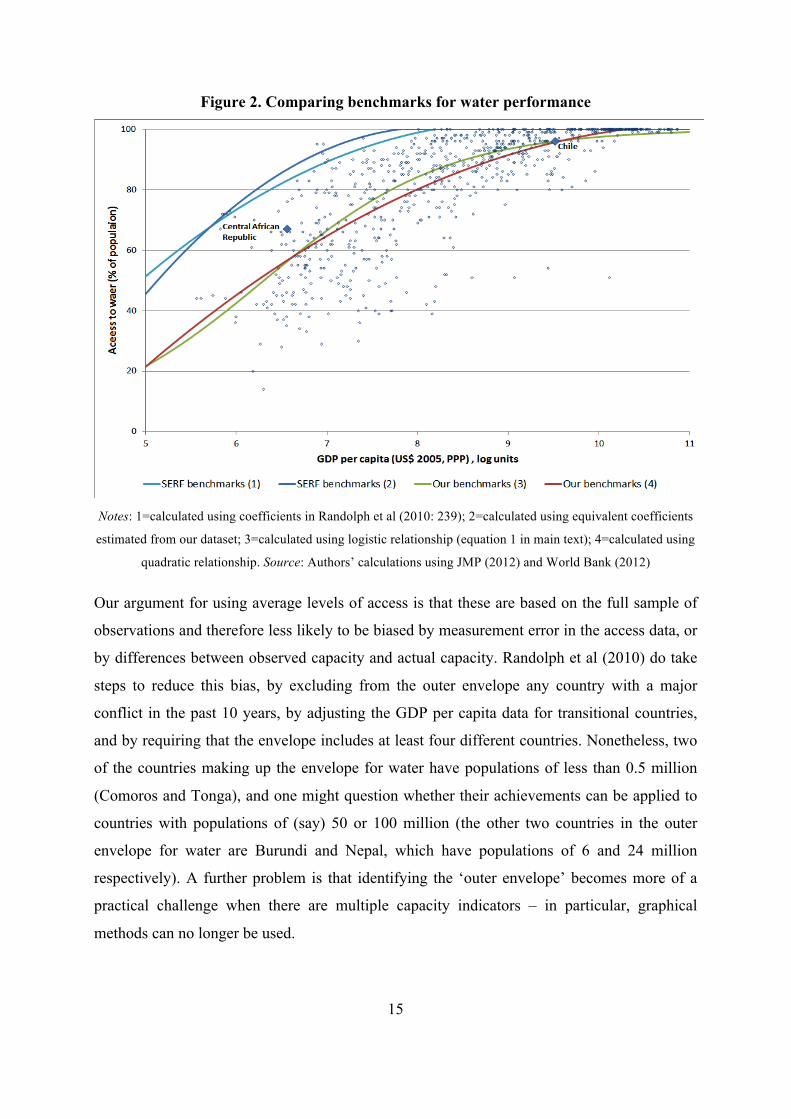
To illustrate, consider Figure 2 which compares the SERF benchmarks with those generated

by a partial version of our approach which for comparative purposes uses GDP per capita as

the only capacity indicator. As expected, the SERF benchmarks are higher than our

benchmarks at all levels of GDP per capita; however, the extent of the difference is much

larger at lower levels of GDP per capita than at higher levels.20 This difference in slope in turn

leads to different rankings. For example, access to water in the Central African Republic in

2010 was (at 67 per cent) above average for its level of GDP per capita, but in Chile it was (at

96 per cent) roughly equal to the average. Thus by our approach, the Central African Republic

is performing better than Chile, controlling for capacity (in this case, just GDP per capita).

However, Chile is closer to its estimated highest achievable level of access than the Central

African Republic. Thus according to the SERF index, Chile is performing better than the

Central African Republic.

20 Note that the SERF bencharks assume a quadratic relationship between the highest level of access and GDP per capita, in contrast to our assumption of a logistic relationship between average levels of access and GDP per capita. However, if we also assume a quadratic relationship, our benchmarks are very similar to those derived under the assumption of a logistic relationship (see Figure 2). Note also that since our dataset differs somewhat from that used by Randolph et al (2010), we re-estimated the relationship between GDP per capita and the highest achievable level of access, using an otherwise identical methodology; the results are again very similar (see Figure 2).

15

Figure 2. Comparing benchmarks for water performance

Notes: 1=calculated using coefficients in Randolph et al (2010: 239); 2=calculated using equivalent coefficients

estimated from our dataset; 3=calculated using logistic relationship (equation 1 in main text); 4=calculated using

quadratic relationship. Source: Authors’ calculations using JMP (2012) and World Bank (2012)

Our argument for using average levels of access is that these are based on the full sample of

observations and therefore less likely to be biased by measurement error in the access data, or

by differences between observed capacity and actual capacity. Randolph et al (2010) do take

steps to reduce this bias, by excluding from the outer envelope any country with a major

conflict in the past 10 years, by adjusting the GDP per capita data for transitional countries,

and by requiring that the envelope includes at least four different countries. Nonetheless, two

of the countries making up the envelope for water have populations of less than 0.5 million

(Comoros and Tonga), and one might question whether their achievements can be applied to

countries with populations of (say) 50 or 100 million (the other two countries in the outer

envelope for water are Burundi and Nepal, which have populations of 6 and 24 million

respectively). A further problem is that identifying the ‘outer envelope’ becomes more of a

practical challenge when there are multiple capacity indicators – in particular, graphical

methods can no longer be used.

16

Of course, the average level of performance could be below the level of access that a country

could achieve if it took its commitments seriously. However, the same also applies to states

making up the outer envelope. While they are obviously doing better than other countries,

given their capacity, we cannot necessarily assume that they are doing as well as they could

be: if, for instance, they are using their ‘maximum available resources’ in order to achieve the

highest possible level of access to water and sanitation, given their capacity.

The second way in which we apply our approach is to rank countries on the basis of their

trends in performance since 1990, the starting date for the MDG targets. The trend in

performance is given by:

∑−

−−

=−

k

ikTikk

iTiiTi

nXX

nAA

nzz )(ˆ 90,,90,,90,, β (5)

where T is the latest available year of data and n is the length of the period in years. The trend

in performance is therefore the sum of two parts: the actual change in access over the period

minus an adjustment for changes in each capacity indicator over the period.

Applied in this way, our approach has parallels with MDG performance assessments which

compare countries in terms of whether and to what extent they are ‘on-track’ or ‘off-track’

towards the goal of halving the proportion of the population lacking access to water and

sanitation between 1990 and 2015. This target translates into a required rate of reduction of

2.8 per cent per year; thus countries with higher actual rates of reduction since 1990 are

considered to be good performers while countries with lower rates of reduction are considered

poor performers – in each case, increasingly so as rates of reduction lie above or below this

threshold. The implicit performance measure is therefore:

⎟⎟⎠

⎞⎜⎜⎝

⎛=

Ti

iMDGi s

sn

z,

90,ln1 (6)

where si is the percentage of the population without access.

There are however two key differences between this second application of our approach and

MDG performance assessments. First, our approach adjusts for trends in state capacity,

whereas MDG performance assessments do not. Thus countries in which the capacity

17

indicators have grown strongly since 1990 will tend to be ranked lower by our measure than

by an MDG assessment, ceteris paribus. Second, unlike MDG assessments, our approach is

not limited to rates of reduction in the proportion of the population lacking access to water

and sanitation; we also consider rates of increase in the proportion with access. To see this,

note that the annualised change in access measured as a log-odds ratio can be re-written as:

⎟⎟⎠

⎞⎜⎜⎝

⎛+⎟⎟⎠

⎞⎜⎜⎝

⎛=

−

Ti

i

i

TiiTi

ss

naa

nnAA

,

90,

90,

,90,, ln1ln1 (7)

where ai is the percentage of the population with access. Thus if capacity remains constant,

performance is equal to the proportional increase in the proportion with access plus the

proportional decrease in the proportion without access. This is of relevance since the MDG

target for water and sanitation has been criticised for focusing only on the proportional

reduction in the proportion without access, since this disadvantages regions (e.g. Sub Saharan

Africa) where the proportion without access is higher. For example, according to Easterly

(2008: 32), “percentage changes are higher when one starts from a lower base, which gives

the advantage to other regions on WITHOUT [access] and the advantage to Africa on WITH

[access].”

18

3.  Comparing  performance  across  countries    

3.1  Regression  results:  access  and  capacity  

We first report estimates of the effects of the six capacity indicators discussed in Section 2 on

access to water and sanitation. Sample information and descriptive statistics for each variable

are shown in Table 1. Our sample includes data for 138 countries, with data at 5-year intervals

between 1990 and 2010 (maximum of five observations per country). Observations where

access is equal to 100 per cent are excluded since the log-odds ratio is not defined in these

cases. The estimation method is ordinary least squares.

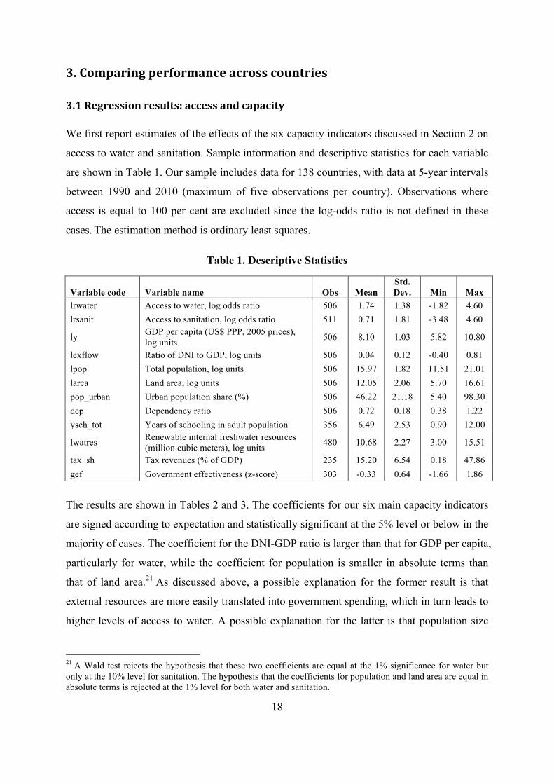
Table 1. Descriptive Statistics

Variable code Variable name Obs Mean Std. Dev. Min Max

lrwater Access to water, log odds ratio 506 1.74 1.38 -1.82 4.60 lrsanit Access to sanitation, log odds ratio 511 0.71 1.81 -3.48 4.60

ly GDP per capita (US$ PPP, 2005 prices), log units 506 8.10 1.03 5.82 10.80

lexflow Ratio of DNI to GDP, log units 506 0.04 0.12 -0.40 0.81 lpop Total population, log units 506 15.97 1.82 11.51 21.01 larea Land area, log units 506 12.05 2.06 5.70 16.61 pop_urban Urban population share (%) 506 46.22 21.18 5.40 98.30 dep Dependency ratio 506 0.72 0.18 0.38 1.22 ysch_tot Years of schooling in adult population 356 6.49 2.53 0.90 12.00

lwatres Renewable internal freshwater resources (million cubic meters), log units 480 10.68 2.27 3.00 15.51

tax_sh Tax revenues (% of GDP) 235 15.20 6.54 0.18 47.86 gef Government effectiveness (z-score) 303 -0.33 0.64 -1.66 1.86

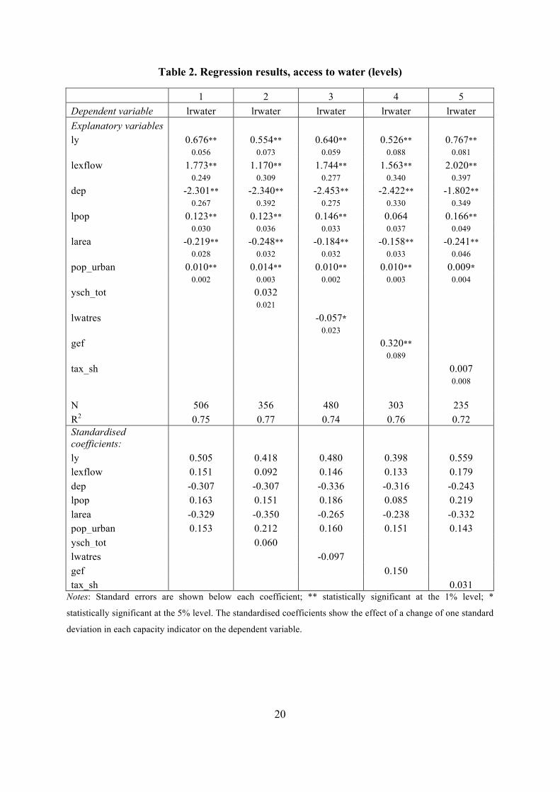
The results are shown in Tables 2 and 3. The coefficients for our six main capacity indicators

are signed according to expectation and statistically significant at the 5% level or below in the

majority of cases. The coefficient for the DNI-GDP ratio is larger than that for GDP per capita,

particularly for water, while the coefficient for population is smaller in absolute terms than

that of land area.21 As discussed above, a possible explanation for the former result is that

external resources are more easily translated into government spending, which in turn leads to

higher levels of access to water. A possible explanation for the latter is that population size

21 A Wald test rejects the hypothesis that these two coefficients are equal at the 1% significance for water but only at the 10% level for sanitation. The hypothesis that the coefficients for population and land area are equal in absolute terms is rejected at the 1% level for both water and sanitation.

19

has an additional negative effect on access, above and beyond its positive effect via

population density, due to diseconomies of scale. However, the standardised (beta)

coefficients show that GDP per capita has the largest effect on access by far, followed by the

dependency ratio and land area.22

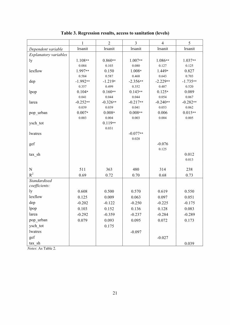
In terms of the other potential capacity indicators, the coefficient for educational attainment is

positive and statistically significant for sanitation, but smaller in size and not statistically

significant for water. The coefficient for domestic resources is negative and statistically

significant for both water and sanitation, which is contrary to expectation. The coefficient for

government effectiveness is positive and statistically significant for access to water, as

expected, but not statistically significant for sanitation. The coefficient for tax revenues is

positive but not statistically significant for water or sanitation. Of these additional indicators,

government effectiveness has the largest impact in standardised terms (at least for water),

although even in this case the effect is smaller than that of GDP per capita, the dependency

ratio or land area. For this reason, including these additional capacity indicators do not

substantially affect our performance rankings (see Section 3.2 below).

22 The standardised (beta) coefficients show the change in access in standard deviations when each capacity indicator changes by one standard deviation.

20

Table 2. Regression results, access to water (levels)

1 2 3 4 5 Dependent variable lrwater lrwater lrwater lrwater lrwater Explanatory variables ly 0.676** 0.554** 0.640** 0.526** 0.767**

0.056 0.073 0.059 0.088 0.081

lexflow 1.773** 1.170** 1.744** 1.563** 2.020**

0.249 0.309 0.277 0.340 0.397

dep -2.301** -2.340** -2.453** -2.422** -1.802**

0.267 0.392 0.275 0.330 0.349

lpop 0.123** 0.123** 0.146** 0.064 0.166**

0.030 0.036 0.033 0.037 0.049

larea -0.219** -0.248** -0.184** -0.158** -0.241**

0.028 0.032 0.032 0.033 0.046

pop_urban 0.010** 0.014** 0.010** 0.010** 0.009*

0.002 0.003 0.002 0.003 0.004

ysch_tot

0.032

0.021

lwatres

-0.057*

0.023

gef

0.320**

0.089

tax_sh

0.007

0.008

N 506 356 480 303 235 R2 0.75 0.77 0.74 0.76 0.72 Standardised coefficients: ly 0.505 0.418 0.480 0.398 0.559 lexflow 0.151 0.092 0.146 0.133 0.179 dep -0.307 -0.307 -0.336 -0.316 -0.243 lpop 0.163 0.151 0.186 0.085 0.219 larea -0.329 -0.350 -0.265 -0.238 -0.332 pop_urban 0.153 0.212 0.160 0.151 0.143 ysch_tot 0.060 lwatres -0.097 gef 0.150 tax_sh 0.031

Notes: Standard errors are shown below each coefficient; ** statistically significant at the 1% level; *

statistically significant at the 5% level. The standardised coefficients show the effect of a change of one standard

deviation in each capacity indicator on the dependent variable.

21

Table 3. Regression results, access to sanitation (levels)

1 2 3 4 5 Dependent variable lrsanit lrsanit lrsanit lrsanit lrsanit Explanatory variables ly 1.108** 0.860** 1.007** 1.086** 1.037**

0.084 0.103 0.080 0.127 0.125 lexflow 1.997** 0.150 1.008* 1.449* 0.827

0.584 0.587 0.468 0.643 0.703 dep -1.992** -1.219* -2.356** -2.229** -1.735**

0.357 0.499 0.352 0.487 0.520 lpop 0.104* 0.160** 0.143** 0.125* 0.089

0.041 0.044 0.044 0.054 0.067 larea -0.252** -0.326** -0.217** -0.240** -0.282**

0.039 0.039 0.041 0.053 0.062 pop_urban 0.007* 0.008* 0.008** 0.006 0.015**

0.003 0.004 0.003 0.004 0.005 ysch_tot 0.119** 0.031 lwatres -0.077** 0.028 gef -0.076 0.125 tax_sh 0.012

0.013

N 511 363 480 314 238 R2 0.69 0.72 0.70 0.68 0.73 Standardised coefficients: ly 0.608 0.500 0.570 0.619 0.550 lexflow 0.125 0.009 0.063 0.097 0.051 dep -0.202 -0.122 -0.250 -0.225 -0.175 lpop 0.103 0.152 0.136 0.128 0.083 larea -0.292 -0.359 -0.237 -0.284 -0.289 pop_urban 0.079 0.093 0.095 0.072 0.173 ysch_tot 0.175 lwatres -0.097 gef -0.027 tax_sh 0.039

Notes: As Table 2.

22

3.2  Country  rankings  

In this section we present our country rankings in terms of levels of performance in the most

available year of data: either 2010 or 2005. Our performance measure is given by the

difference between the actual level of access and the predicted level of access on the basis of

the observable capacity indicators (equation 2 in Section 2). As discussed in Section 2, we

exclude from the calculations any countries in which access is equal to 100 per cent; some

countries are also excluded due to missing data. Overall we are able to calculate our

performance measure for 114 countries for water and 121 countries for sanitation, of which 81

and 84 have data for 2010.23

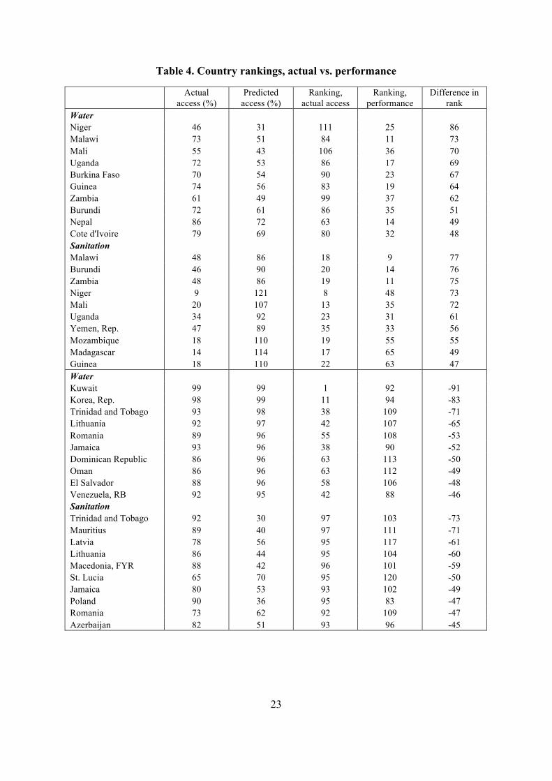
The full set of results for each country is shown in Appendix 2; here we focus on the key

overall findings. First, our performance rankings have only a moderate correlation with

rankings based on observed levels of access: the Spearman rank correlation coefficients are

0.49 for water and 0.56 for sanitation. The absence of a strong correlation is due to two

factors. On the one hand, there are countries, predominantly in sub-Saharan Africa, in which

access is relatively low but predicted access is also low if not lower. These countries rank

much higher by our measure than they do by access alone; examples include Niger, Malawi,

Mali, and Uganda (see Table 4). On the other hand, there are countries, predominantly

middle-income, in which access is relatively high but predicted access si even higher. These

countries rank much lower by our measure than by their unadjusted level of access; examples

include Kuwait, South Korea, Trinidad and Tobago, and Lithuania (see again Table 4).

Overall, controlling for capacity clearly makes a significant difference to how we judge

‘good’ performance.

23 We found no tendency for levels of access to be higher in 2010 than in 2005, controlling for the capacity indicators. This suggests that there is no bias in our rankings against the countries in our samples which do not yet have data for 2010.

23

Table 4. Country rankings, actual vs. performance

Actual access (%)

Predicted access (%)

Ranking, actual access

Ranking, performance

Difference in rank

Water Niger 46 31 111 25 86

Malawi 73 51 84 11 73 Mali 55 43 106 36 70 Uganda 72 53 86 17 69 Burkina Faso 70 54 90 23 67 Guinea 74 56 83 19 64 Zambia 61 49 99 37 62 Burundi 72 61 86 35 51 Nepal 86 72 63 14 49 Cote d'Ivoire 79 69 80 32 48 Sanitation

Malawi 48 86 18 9 77 Burundi 46 90 20 14 76 Zambia 48 86 19 11 75 Niger 9 121 8 48 73 Mali 20 107 13 35 72 Uganda 34 92 23 31 61 Yemen, Rep. 47 89 35 33 56 Mozambique 18 110 19 55 55 Madagascar 14 114 17 65 49 Guinea 18 110 22 63 47 Water

Kuwait 99 99 1 92 -91 Korea, Rep. 98 99 11 94 -83 Trinidad and Tobago 93 98 38 109 -71 Lithuania 92 97 42 107 -65 Romania 89 96 55 108 -53 Jamaica 93 96 38 90 -52 Dominican Republic 86 96 63 113 -50 Oman 86 96 63 112 -49 El Salvador 88 96 58 106 -48 Venezuela, RB 92 95 42 88 -46 Sanitation

Trinidad and Tobago 92 30 97 103 -73 Mauritius 89 40 97 111 -71 Latvia 78 56 95 117 -61 Lithuania 86 44 95 104 -60 Macedonia, FYR 88 42 96 101 -59 St. Lucia 65 70 95 120 -50 Jamaica 80 53 93 102 -49 Poland 90 36 95 83 -47 Romania 73 62 92 109 -47 Azerbaijan 82 51 93 96 -45

24

Second, our performance rankings show no significant correlation with any of the six main

capacity indicators. There is for example no tendency for countries with higher levels of GDP

per capita to receive higher performance scores: the rank correlation is less than 0.10 in all

cases, and is never statistically significant. Relatedly, we find no evidence that rankings differ

significantly between low-income, middle-income and high-income countries: an F-test of the

equality of the average ranks across income groups cannot be rejected at the 10% level for

both water and sanitation. Put more simply, state performance and state capacity are in our

approach unrelated: there is no tendency for states with greater capacity to perform better than

states with lesser capacity.

Third, our use of multiple capacity indicators does make a difference. The correlation between

our rankings and those generated by an identical approach with GDP as the only capacity

indicator is high – 0.78 for water and 0.85 for sanitation – but clearly not perfect. For example,

Zambia is ranked 89th out of 114 countries in terms of its water performance when including

only GDP per capita, but it is ranked 37th when adding the other five capacity indicators. One

of the reasons for this difference is that disposable national income (DNI) in Zambia is quite a

bit below its GDP, because of repatriated earnings on foreign direct investment. Similarly, the

Republic of Congo rises from 103rd to 44th place, again mainly because of its low level of DNI

relative to GDP.

Finally, we re-estimated our rankings including each of the other possible capacity indicators

discussed in Section 2: education attainments, domestic water resources, tax revenues, and

government effectiveness. In each case, the rankings are very similar to those based on our six

main capacity indicators: the Spearman rank correlation coefficients are all above 0.97. This

reflects the finding of the regression analysis in Section 3.1, namely that the effect of these

other indicators on average levels of access is smaller, in standardised terms, than our main

capacity indicators. Thus while state capacity can never be measured exactly, our rankings do

at least appear to be robust to the particular indicators of capacity chosen from the set of

potential indicators available in standard international datasets.

3.3  Comparison  with  SERF  index  

We now compare our rankings with those generated by the SERF index (Randolph, Fukuda-

Parr and Lawson-Remer, 2010). As noted in Section 2, this index also ranks states on the

25

basis of levels of performance, adjusting for state capacity, but differs from our approach in

certain key ways: it uses a single capacity indicator, GDP per capita, and estimates

benchmarks on the basis of highest observed level of access at any given level of GDP per

capita, rather than the average level. We confine our comparison to the SERF performance

indices for water and sanitation, which are just two of the 13 outcome indicators considered

by the overall SERF index.

The benchmarks for water and sanitation used by the SERF index are estimated by regression

analysis applied to the outer envelope of observations. This method yields the following

formulae:

2

210 lnln ⎥⎦

⎤⎢⎣

⎡⎟⎠

⎞⎜⎝

⎛+⎟⎠

⎞⎜⎝

⎛+=POPGDP

POPGDPAi χχχ (water)

1

0

δ

δ ⎟⎠

⎞⎜⎝

⎛=POPGDPAi (sanitation)

with coefficients 88.1510 −=χ , 14.561 =χ , 10.32 −=χ and 04.90 =δ and 29.01 =δ (Randolph et al 2010: 239). The benchmarks are capped at 100 per cent in each case. Since

our dataset differs somewhat from that used by Randolph et al (2010), we re-estimated the

coefficients using our dataset and an otherwise identical methodology, yielding coefficients

49.2,13.47,0.116 210 −==−= χχχ and 381.0,824.4 10 == δδ . In what follows we report

the comparison using the original coefficients reported by Randolph et al, but the results are

very similar using our re-estimated coefficients.

The rank correlation between our measure and the SERF index is 0.59 for water and 0.71 for

sanitation. Part of the reason for the difference is our use of multiple capacity indicators: if we

compare the partial version of our measure, which includes GDP per capita as the single

capacity indicator, the rank correlations rise to 0.81 for water and 0.83 for sanitation. Given

the uncertainties of any performance exercise, some differences in rankings between

alternative approaches are of course to be expected. Nevertheless, the differences between our

approach and the SERF index are systematic: countries with lower GDP per capita tend to be

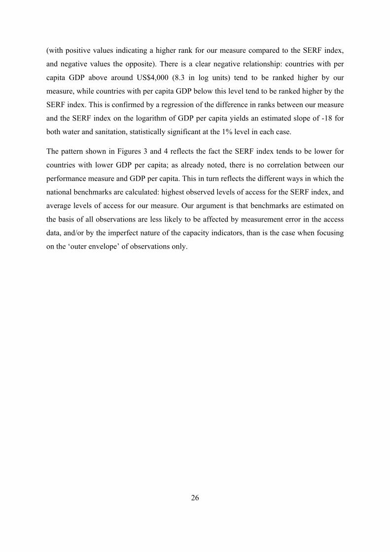
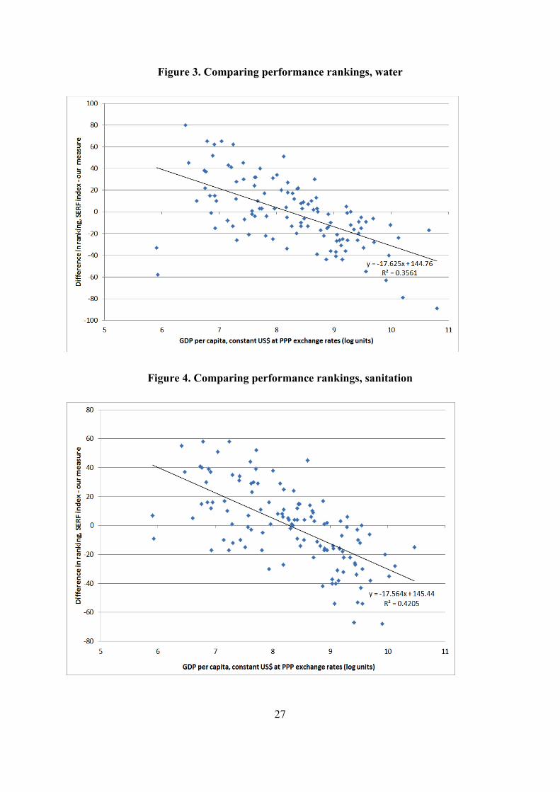
ranked substantially higher by our measure compared with the SERF index. This is shown by

Figures 3 and 4, which plot the difference in country rankings between the two measures

26

(with positive values indicating a higher rank for our measure compared to the SERF index,

and negative values the opposite). There is a clear negative relationship: countries with per

capita GDP above around US$4,000 (8.3 in log units) tend to be ranked higher by our

measure, while countries with per capita GDP below this level tend to be ranked higher by the

SERF index. This is confirmed by a regression of the difference in ranks between our measure

and the SERF index on the logarithm of GDP per capita yields an estimated slope of -18 for

both water and sanitation, statistically significant at the 1% level in each case.

The pattern shown in Figures 3 and 4 reflects the fact the SERF index tends to be lower for

countries with lower GDP per capita; as already noted, there is no correlation between our

performance measure and GDP per capita. This in turn reflects the different ways in which the

national benchmarks are calculated: highest observed levels of access for the SERF index, and

average levels of access for our measure. Our argument is that benchmarks are estimated on

the basis of all observations are less likely to be affected by measurement error in the access

data, and/or by the imperfect nature of the capacity indicators, than is the case when focusing

on the ‘outer envelope’ of observations only.

27

Figure 3. Comparing performance rankings, water

 

Figure 4. Comparing performance rankings, sanitation

28

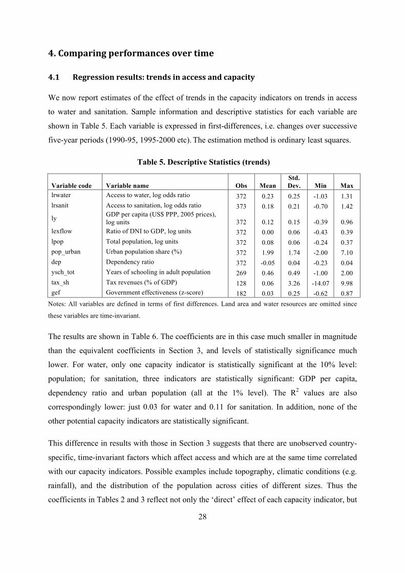
4.  Comparing  performances  over  time  

4.1   Regression  results:  trends  in  access  and  capacity    

We now report estimates of the effect of trends in the capacity indicators on trends in access

to water and sanitation. Sample information and descriptive statistics for each variable are

shown in Table 5. Each variable is expressed in first-differences, i.e. changes over successive

five-year periods (1990-95, 1995-2000 etc). The estimation method is ordinary least squares.

Table 5. Descriptive Statistics (trends)

Variable code Variable name Obs Mean Std. Dev. Min Max

lrwater Access to water, log odds ratio 372 0.23 0.25 -1.03 1.31 lrsanit Access to sanitation, log odds ratio 373 0.18 0.21 -0.70 1.42

ly GDP per capita (US$ PPP, 2005 prices), log units 372 0.12 0.15 -0.39 0.96

lexflow Ratio of DNI to GDP, log units 372 0.00 0.06 -0.43 0.39 lpop Total population, log units 372 0.08 0.06 -0.24 0.37 pop_urban Urban population share (%) 372 1.99 1.74 -2.00 7.10 dep Dependency ratio 372 -0.05 0.04 -0.23 0.04 ysch_tot Years of schooling in adult population 269 0.46 0.49 -1.00 2.00 tax_sh Tax revenues (% of GDP) 128 0.06 3.26 -14.07 9.98 gef Government effectiveness (z-score) 182 0.03 0.25 -0.62 0.87

Notes: All variables are defined in terms of first differences. Land area and water resources are omitted since

these variables are time-invariant.

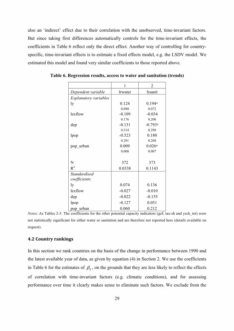
The results are shown in Table 6. The coefficients are in this case much smaller in magnitude

than the equivalent coefficients in Section 3, and levels of statistically significance much

lower. For water, only one capacity indicator is statistically significant at the 10% level:

population; for sanitation, three indicators are statistically significant: GDP per capita,

dependency ratio and urban population (all at the 1% level). The R2 values are also

correspondingly lower: just 0.03 for water and 0.11 for sanitation. In addition, none of the

other potential capacity indicators are statistically significant.

This difference in results with those in Section 3 suggests that there are unobserved country-

specific, time-invariant factors which affect access and which are at the same time correlated

with our capacity indicators. Possible examples include topography, climatic conditions (e.g.

rainfall), and the distribution of the population across cities of different sizes. Thus the

coefficients in Tables 2 and 3 reflect not only the ‘direct’ effect of each capacity indicator, but

29

also an ‘indirect’ effect due to their correlation with the unobserved, time-invariant factors.

But since taking first differences automatically controls for the time-invariant effects, the

coefficients in Table 6 reflect only the direct effect. Another way of controlling for country-

specific, time-invariant effects is to estimate a fixed effects model, e.g. the LSDV model. We

estimated this model and found very similar coefficients to those reported above.

Table 6. Regression results, access to water and sanitation (trends)

1 2 Dependent variable lrwater lrsanit Explanatory variables ly 0.124 0.194*

0.080 0.072 lexflow -0.109 -0.034

0.176 0.200 dep -0.131 -0.793*

0.314 0.298 lpop -0.523 0.180

0.291 0.208 pop_urban 0.009 0.026*

0.008 0.007 N 372 373 R2 0.0338 0.1143 Standardised coefficients: ly 0.074 0.136 lexflow -0.027 -0.010 dep -0.022 -0.155 lpop -0.127 0.051 pop_urban 0.060 0.212

Notes: As Tables 2-3. The coefficients for the other potential capacity indicators (gef, tax-sh and ysch_tot) were

not statistically significant for either water or sanitation and are therefore not reported here (details available on

request).

4.2  Country  rankings  

In this section we rank countries on the basis of the change in performance between 1990 and

the latest available year of data, as given by equation (4) in Section 2. We use the coefficients

in Table 6 for the estimates of kβ , on the grounds that they are less likely to reflect the effects

of correlation with time-invariant factors (e.g. climatic conditions), and for assessing

performance over time it clearly makes sense to eliminate such factors. We exclude from the

30

analysis any countries with levels of access equal to 100 per cent in the latest available year;

some countries are also excluded due to missing data. Overall, we are able to calculate

changes in performance for 80 countries for water and 79 for sanitation; the latest available

year is 2010 in 58 and 57 cases respectively; in all other cases it is 2005. The full rankings are

shown in Appendix 2; here we focus on the key overall findings.

The main result is that our rankings of countries on the basis of changes in performance are

much less affected by capacity than those in Section 3: our rankings are quite similar to those

yielded simply on the basis of the actual changes in access over time: 0.92 for sanitation and

0.98 for water. This reflects the more limited explanatory power that our capacity indicators

have in explaining changes in levels of access over time, as evidenced in the relatively low R2

figures for the regressions in first difference form in Table 6. Nevertheless, we still find some

significant differences between our rankings and those generated by MDG performance

assessments.

4.3  Comparison  with  MDG  performance  assessments  

As noted in Section 2, the implicit performance measure for water and sanitation in the

current MDG framework is the average annual rate of reduction in the proportion of the

population lacking access to water or sanitation between 1990 and the latest available year of

data. Our measure of the trend in performance differs for two reasons: first, it adjusts for

changes in capacity, and second it includes the proportional increase in the proportion of the

population with access as well as the proportional decrease in the proportion of the population

without access.

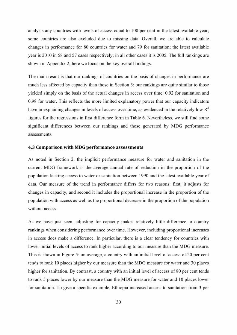
As we have just seen, adjusting for capacity makes relatively little difference to country

rankings when considering performance over time. However, including proportional increases

in access does make a difference. In particular, there is a clear tendency for countries with

lower initial levels of access to rank higher according to our measure than the MDG measure.

This is shown in Figure 5: on average, a country with an initial level of access of 20 per cent

tends to rank 10 places higher by our measure than the MDG measure for water and 30 places

higher for sanitation. By contrast, a country with an initial level of access of 80 per cent tends

to rank 5 places lower by our measure than the MDG measure for water and 10 places lower

for sanitation. To give a specific example, Ethiopia increased access to sanitation from 3 per

31

cent in 1990 to 21 per cent in 2010. This ranks in only 45th place (out of 79 countries)

according to the MDG measure of performance, the percentage reduction in the proportion of

the population without access (just 1 per cent per year between 1990 and 2010). But Ethiopia

ranks 2nd out of 79 countries by our approach, which factors in the percentage increase in the

proportion of the population with access (10 per cent year between 1990 and 2010). This

gives an indication of the amount of bias resulting from the apparently arbitrary focus by the

MDGs on rates of decrease in access shortfalls, and the exclusion of information on rates of

increase in access.

Figure 5. Comparing performance rankings, water and sanitation (trends)

There are also systematic differences between our rankings and MDG rankings when we

compare countries by income group and by region. Using the World Bank’s classification

system, low-income countries tend to be ranked higher by our measure than the MDG

measure; by contrast, lower and upper middle income countries tend to be ranked lower by

our measure than the MDG measure. These differences mainly reflect the fact that low-

income countries had (on average) lower levels of access in 1990; lower rates of economic

growth among low-income countries also play a role in explaining the differences, but only

for sanitation. The same conclusion applies if we group countries into quintiles based on the

32

level of GDP per capita; lower-income groups tend to be ranked higher by our measure than

the MDG measure, and vice versa for higher-income groups. For the results by region,

countries in Sub-Saharan Africa tend to be ranked higher according to our measure than the

MDG measure. This again mainly reflects the lower average level of access in Sub-Saharan

Africa in 1990, and partly (at least for sanitation) the slower average rate of economic growth

since 1990. In the last few years, economic growth has accelerated in sub-Saharan the Africa

and it will be interesting to reassess the resource-adjusted performance in the coming years.

33

5.  Conclusion:  Towards  the  Post-­‐2015  Agenda  

The MDG monitoring framework has been critiqued for penalising low-income countries and

favouring middle-income countries. The former are burdened with a more constrained

resource envelope and the task of halving or eliminating significantly higher shortfalls. Even

if unintended, this bias in the MDGs metric becomes clear once it is subjected to quantitative

analysis. As our analysis makes clear in the case of water and sanitation, an adjustment for

capacity reveals a partial bias against low-income countries. The ranking of countries shifts

with a number of low-income countries rising up the performance ladder and a number of

middle-income countries fall. When we focus on changes in performance, we reveal a bias

against countries with low levels of access – mainly low income countries. While we would

be cautious about replacing the existing MDGs rankings with our approach – one needs to be

careful about the use of global rankings - the results point to an underlying problem when the

MDGs framework is used as a cross-national monitoring measure.

In the emerging discussions on a new global development agenda, there is a recognition that

any post-2015 goals will need to fairer across countries. This will be crucial for their

legitimacy. In the 2012 Rio Declaration, States set parameters for establishing Sustainable

Development Goals, which can be read as applicable for the post-2015 agenda. One of the

criteria is that they must be “universally applicable to all countries while taking into account

different national realities, capacities and levels of development”. 24 There is thus a challenge

as to how national capacities are built into the universal benchmarks.

Potentially, one could design a target based on the alternative metrics presented above. If we

took the SERF approach, a country could be on target if it has closed by 50 or 100 per cent the

gap between its current level of access and the maximum level of access for its level of GDP.

However, if the target is ambitious (e.g., over 50 per cent) there will be strong scrutiny and

controversy as to whether its achievement possibility frontier is truly realistic for all countries.

Using an average-based approach as we do, countries could be required to at least achieve the

24 Para. 247. The full sentence reads that the framework should be “action-oriented, concise and easy to communicate, limited in number, global in nature and universally applicable to all countries while taking into account different national realities, capacities and levels of development and respecting national policies and priorities”. It should also “be consistent with international law”, incorporate all dimensions of sustainable development in a balanced and coordinated manner and be implemented “with the active involvement of all relevant stakeholders” (Paras. 246-7).

34

average performance at their level of GDP for the last two decades. But this risks being under-

ambitious. Therefore, a compromise may be to set a standard whereby States are expected to

achieve the average pace of progress for say the five top performers in their general income

bracket.

However, the problem with such proposals is that rely on coefficients generated by

multivariate regression analysis – and GDP is shifting constantly affecting the relevant target.

This complicates standard-setting and can generate different interpretations and disputes over

statistical methods. A better approach may be to take heed of these quantitative results for

resource-adjustment. A bias exists in the measurement framework that needs to be taken into

account. The task is to design simpler but nuanced targets that take resource constraints into

account. One approach might be to graduate targets according to regions or income-brackets.

For instance, we might expect a halving of the water and sanitation gap in low-income

countries or Sub-Saharan Africa by 2030, but a 75 per cent reduction in all other countries. In

other words, one globalises the MDG-plus approach for wealthier countries.

A second approach to differential capacity is to question whether all countries should be

aiming for the ‘improved’ water and sanitation supply standard set by WHO and UNICEF,

and which informs the basis of the MDG measurement. The water and sanitation indicators

used for the MDGs are fairly minimalistic and wealthier countries could have been pushed to

achieve a higher standard, for example piped access. It is clear that for Sub-Saharan Africa, a

clear challenge remains in simply elevating people from unimproved to the minimalist

‘improved’. However, in the Asian regions, there is at least an equal challenge in moving

from ‘improved’ to piped access.25 In Northern Africa and Latin America, there has been a

dramatic and positive change on piped access while in the former communist states of the CIS

there has been regression. Interestingly, in the MDGs framework, many of these poorly

performing wealthier States would be marked as ‘on target’ as the unimproved gap has been

reduced by 50 per cent. Even in developed countries, access to piped water is notably below

universal access. There is therefore a strong case for raising the threshold requirements for

25 For instance, in South-Eastern Asia, between 2000 and 2008, the unimproved number was halved and the number of piped doubled, but a slight majority of the population still sit with improved access. In Southern Asia and Western Asia, there has been no progress in piped access at all (with the number in the improved category remaining constant).

35

water and sanitation access, particular in middle-income countries.26 They might be expected

to halve or close the gap on lack of access to piped water.27

The capacity-based assessment may suggest that standards should be lowered in poor

countries. For example, WHO and UNICEF (2008: 284) demonstrate positive developments

for a range of poorer countries if one uses a ladder of progress instead of a binary cut-off.

Open defecation declines in all regions (24 per cent to 18 per cent) and in Sub-Saharan Africa

(36 to 28 per cent). Half of decline captured in rise of shared facilities, which is not covered

by the MDGs framework (Bartram, 2008).28 Thus, one could develop a target that tracks and

rewards progress over a ladder from below basic access through to adequate access. For

example, a target could be to ensure that 50 per cent of households move up one ladder rung

(except the top) within 5 to 10 years. However, it may be prudent not to shift the sanitation

standard. It may be more appropriate now given higher levels of growth, the recognition of

sanitation as a human right by the General Assembly in 2010, and the enormous health and

economic benefits generated by investments in sanitation.29

Moreover, it is questionable whether one should even consider lowering the standard for

water. There is a strong argument that the water standard should be raised in poor countries:

not to ensure piped access to homes but rather to increase quantity of water secured. The

current means of measurement presume that an individual is able to secure roughly 20 lcpd

given the distance from the home to a water point (Howard and Bartram, 2003). Both the

MDGs and current international human rights law assume that basic household uses will be

prioritised over other water uses. However, research in rural areas suggests that communities

rank uses quite differently: for example, water for key livestock and kitchen gardening is

prioritised over many household uses (Van Koppen, 2013). One possible approach could be to

26 As Bartram (2008: 284) notes: “The evidence base for the health gains from potential sanitation benchmarks remains appallingly weak. Public toilets may be considered a key intermediate step and a means to ensure at least some dignity and safety. But some speak of dangers, especially to women, of rape and assault; and poorly maintained facilities are themselves a danger to health.” He concedes that some wealthier countries may resist this movement, but points out that some of their policymakers have expressed frustration about the irrelevance of the current MDGs framework. 27 Such a target might also be instrumental in pushing progress on other rights and goals, particularly slum upgrading. The current MDG indicators hide the problems of moving to an adequate level of access. However, once data is introduced on access to piped water or toilets, the failure of many States to make (any) progress on securing urban land tenure and support slum-upgrading (Langford, Bartram and Roaf, 2013; Tissington, 2008) is glaringly revealed. 28 Although there is a question of sustainability with overloaded pits. 29 For every dollar invested in sanitation the resulting benefits are estimated to be between 9 and 34 dollars: Albuquerque (2009) and UNDP (2007).

36

set goals for piped water in middle-and high- income countries, but introduce a multiple-use

perspective into the “improved water” standard for lower-income countries, so that productive

uses are captured.

A further alternative or complementary approach is to pay greater attention to equality. In

middle and high-income countries, the core of social challenge is often not scaling up

programmes to generate broad access to basic levels of economic and social rights. Rather, it

is ensuring that the most marginalised members of society share in this distribution: i.e.,

equality. However, only one target in the MDGs framework pays attention to equal access

(Target 3A on gender equality in schooling) and only one target requires universal access

(primary education).30 The result is that these States can pick the ‘low-hanging fruit’ in

meeting the more relative and average-based targets without having to address the most

deeply excluded individuals and groups. Most disadvantaged groups are heavily

overrepresented in poverty statistics. Thus, a target that directs attention to low-income

groups will invariably require addressing individuals facing others forms of discrimination.

There are various ways in which this could be done. The most practical approach would be to

measure progress for lower income quintiles or deciles. One could replace the current

average-based target with an equality-based target that requires the gap for a lower-income

group (e.g., the bottom quintile) to be halved or eliminated. An alternative approach is to

maintain the current average-based targets, but require proportional improvement for lower-

income groups.

A final alternative metric could be the degree of post-2015 acceleration. If goals and targets

are primarily aimed at boosting performance (Langford, 2012), it might be a useful measure.

Fukuda-Parr and Greenstein (2010) test whether this occurred post-2000 and reveal the

(unfortunate) fact that the majority of countries decelerated but also demonstrate that many

poorer countries have made faster progress on water and sanitation than middle-income

countries. In a separate piece, the authors argues that such an approach not only coheres with

the underlying purpose of the MDGs but is consistent with the duty of progressive realisation

in economic, social and cultural rights (Fukuda-Parr and Greenstein, 2013). However, the

difficult with this approach is the time period. For instance a country that achieved very fast

progress between 2000 and 2015 would face a more demanding target than countries that

30 Although the measures for the latter often fail to pick up excluded children with disabilities

37

were more sluggish. Unlike the resource-based approach, it risks being too backward–looking

in determining the measure of performance. This could be overcome by using on the average

rate of performance for various bands of GDP.

In summary, frameworks like the MDGs function best when they blend ambition with realism:

set at standard high enough to inspire action but low enough to be achievable. This is the

baseline provided by international human rights law although failure to reach a bare minimum

for all still requires a particularly strong justification. This suggests that the standard for

access to water and sanitation should be raised in the future for middle-income countries. But

it does not necessarily mean it should be dropped for low-income countries.

38

References  

Albuquerque, Catarina de (2009), Report of the Independent Expert on the issue of human rights obligations related to access to safe drinking water and sanitation, UN Human Rights Council (Sixty-Fifth Session), U.N. Doc. A/12/24 (Sanitation Report).

Alston, Philip (1992), 'The Committee on Economic, Social and Cultural Rights', in Philip Alston (ed.), United Nations and Human Rights: A Critical Appraisal (Oxford: Oxford University Press).

--- (2005), 'Ships Passing in the Night: The Current State of the Human Rights and Development Debate Seen Through the Lens of the Millennium Development Goals', Human Rights Quarterly, 27(3), 755-829.

Amnesty (2010), From Promises to Delivery: Putting Human Rights at the Heart of the Millennium Development Goals, (London: Amnesty International).

Anand, P.B. (2006), Millennium Development Goal 7: An Assessment of Progress with Respect to Water and Sanitation: Legacy, Synergy, Complacency or Policy (UNU-Wider Research Paper No. 2006/01).

Antrobus, Peggy (2003), 'MDGs—The Most Distracting Gimmick', Seeking accountability on Women’s Human Rights: Women Debate the UN Millennium Development Goals. WICEJ. 2004. (WICEJ), 14-15.

Atkinson, A.B. (2006), 'Funding the Millennium Development Goals: A Challenge for Global Public Finance', European Review, 14(4), 555-64.

Bartram, Jamie (2008), 'Improving on haves and have-nots', Nature, 452, 283-84.

Bourguignon, François , Agnès Bénassy-Quéré, Stefan Dercon, Antonio Estache, Jan Willem Gunning, Ravi Kanbur, Stephan Klasen, Simon Maxwell, Jean-Philippe Platteau, and Amedeo Spadaro (2008), Millennium Development Goals at Midpoint: Where do we stand and where do we need to go?, Background paper for European Report on Development Avaialble at http://ec.europa.eu/development/icenter/repository/mdg_paper_final_20080916_en.pdf [Accessed 2 December 2010].

Chakravarty, Satya and Amita Majumber (2008), 'Millennium Development Goals: Measuring Progress Towards their Achievement', Journal of Humanitarian Development, 9(1), 109-29.

Dugard, Jackie, Malcolm Langford, and Edward Anderson (2013), 'Determining Progress on Access to Water and Sanitation: Law and Political Economy in South Africa', in Malcolm Langford and Anna Russell (eds.), The Right to Water: Theory, Practice and Prospects (Cambridge: Cambridge University Press).

Easterly, William (2009), 'How the Millennium Development Goals are Unfair to Africa', World Development, 37(1), 26-35.

Felner, Eitan (2009), 'Closing the ‘Escape Hatch’: A Toolkit to Monitor the Progressive Realization of Economic, Social, and Cultural Rights', Journal of Human Rights Practice, 1(3), 402-35.

Fukuda-Parr, Sakiko and Joshua Greenstein (2010), How Should MDG Implementation Be Measured: Faster Progress or Meeting Targets?,, ed. Working Paper ( Brasilia: International Policy Centre for Inclusive Growth).

39

--- (2013), 'Monitoring MDGs: A Human Rights Critique and Alternative', in Malcolm Langford, Andrew Sumner, and Alicia Ely Yamin (eds.), The MDGs and Human Rights: Past, Present and Future (Cambridge: Cambridge University Press).

Howard, Guy and Jamie Bartram (2003), Domestic Water Quantity, Service Level and Health (Geneva: WHO, WHO/SDE/WSH/03.02)).

Hutton, Guy and Laurence Haller (2004), Evaluation of the Costs and Benefits of Water and Sanitation Improvements at the Global Level (Geneva: WHO).

Krause, Matthias (2009), The Political Economy of Water and Sanitation (London: Routledge).

Langford, Malcolm (2010), 'A Poverty of Rights: Six Ways to Fix the MDGs', IDS Bulletin, 41(1), 83-91.

--- (2012), 'The Art of the Impossible: Measurement Choices and the Post-2015 Development Agenda', Background Paper for Governance and human rights: Criteria and measurement proposals for a post-2015 development agenda, OHCHR/UNDP Expert Consultation, New York, 13-14 November

Langford, Malcolm and Jeff A. King (2008), 'Committee on Economic, Social and Cultural Rights: Past, Present and Future', in Malcolm Langford (ed.), Social Rights Jurisprudence: Emerging Trends in International and Comparative Law (Cambridge: Cambridge University Press), 477-516.

Langford, Malcolm and Anna Russell (eds.) (2013), The Right to Water: Theory, Practice and Prospects (Cambridge: Cambridge University Press).

Mboup, G. (2005), Existing Indicators in the Water and Sanitation Sector: Indicators for Accessibility, Affordability and Non-Discrimination eds Virginia Roaf, Ashfaq Khalfan, and Malcolm Langford (Indicators for the Right to Water: Concept Paper No. 13).

OHCHR (2010), Human Rights and MDGs in Practice: A review of country strategies and reporting (Geneva: OHCHR).

Pogge, Thomas (2004), 'The First United Nations Millennium Development Goal: a cause for celebration?', Journal of Human Development, 5(5), 377-97.

Rajkumar, Andrew Sunil and Vinaya Swaroop (2002), 'Public spending and outcomes: Does governance matter?', Journal of Development Economics, 86(1), 96-111.

Randolph, Susan, Sakiko Fukuda-Parr, and Terra Lawson-Remer (2010), 'Economic and Social Rights Fulfillment Index: Country Scores and Rankings', Journal of Human Rights, 9(3), 230-61.

Singh, Nandita (2013), 'Socio-Cultural Norms, Human Rights and Access to Water and Sanitation', in Malcolm Langford and Anna Russell (eds.), The Right to Water: Theory, Practice and Prospects (Cambridge: Cambridge University Press).

Smets, Henri (2009), De l’eau potable à un prix abordable (Paris: Johanet).

Sumner, Andy and Claire Melamed (2010), 'Introduction - The MDGs and Beyond: Pro-Poor Policy in a Changing World', IDS Bulletin, 41(1), 1-6.

Tabatabai, Hamid (2007), 'MDG Targets: Misunderstood or Misconceived?', International Poverty Centre One-Pager, April.

UN-OHCHR (2008), Claiming the MDGS: A Human Rights Approach (Geneva: Office of the UN High Commissioner for Human Rights).

40

UNDP, WHO and (2007), Economic and health effects of increasing coverage of low cost household drinking-water supply and sanitation interventions to countries off-track to meet MDG target 1 (Geneva: WHO, UN doc. WHO/SDE/WSH/07/0).

UNIFEM (2004), Pathway to Gender Equality: CEDAW, Beijing and the MDGs (New York: UNIFEM).

Van Koppen, Barbara (2013), 'Water Allocation, Customary Practice and the Right to Water: Rethinking the Regulatory Model', in Malcolm Langford and Anna Russell (eds.), The Right to Water: Theory, Practice and Prospects (Cambridge: Cambridge University Press).

Vandemoortele, Jan (2007), 'MDGS: Misunderstood Targets', International Poverty Centre One-Pager, January.

--- (2011), 'The MDG Story: Intention Denied', Development and Change, 43(1), 1-21.

Wolf, Susanna (2007), 'Does Aid Improve Public Service Delivery?', Review of World Economics, 143(4), 650-72.

41

Appendix 1. Absolute vs. relative performance benchmarks

What might constitute an absolute performance benchmark? This section sets out two possible

options. One is the ‘maximum achievable’ level of access: an achievement ceiling beyond

which further achievements are not possible. At least in theory, this will be achieved if raising

access to water and sanitation is the government’s only objective. The other is the ‘minimum

reasonable’ level of access: an achievement floor which will be exceeded if raising access is

one of the government’s objectives, alongside a set of other legitimate objectives (e.g. better

health, education). This level of access will be higher, the greater are complementarities

between access to water and sanitation and other social goals – for example, the extent to

which better access to water and sanitation contributes to better health and higher economic

productivity. For instance, Hutton and Haller (2004) estimate that in developing regions, for

every dollar invested in safe drinking water and sanitation, there were economic and health

returns of $US5 to $US28, depending on the region, technology and cost assumptions.31

The maximum achievable and minimum reasonable levels of access can be illustrated

graphically using an adapted version of the production possibility frontier, a widely used

diagrammatic tool in economics (see Figure A1). The vertical axis shows access to water and

sanitation, while the horizontal axis shows achievements in terms of other legitimate social

goals. The frontier (i.e., the curved line) illustrates the highest possible level of access to

water and sanitation at any given level of achievement in the other goals. The maximum

achievable level of access (denoted maxA ) is given by the highest point of the frontier; the

minimum reasonable level of access (denoted minA ) is given by the level of access at which

the other social goals are maximised. Complementarity between water and sanitation and

other social goals is illustrated by the upward sloping sections of the frontier. In the extreme

case of perfect complementarity, the frontier is an upward sloping line (of fixed length), and minmax AA = ; if there is no complementarity, the possibility curve is always downward sloping

and 0min =A .The shape of the frontier in Figure A1 indicates substantial but not perfect

complementarity.

31 The lower figure is commonly quoted as a global figure. In his cross-country analysis, Anand (2006: 19) concluded that access to water and sanitation has a “highly significant impact on child mortality rate” and to a lesser degree on maternal mortality and incidence of malaria. Rajkumar and Swaroop find a similar but not significant relationship with infant mortality while Wolf (2007) strikingly finds the opposite relationship.

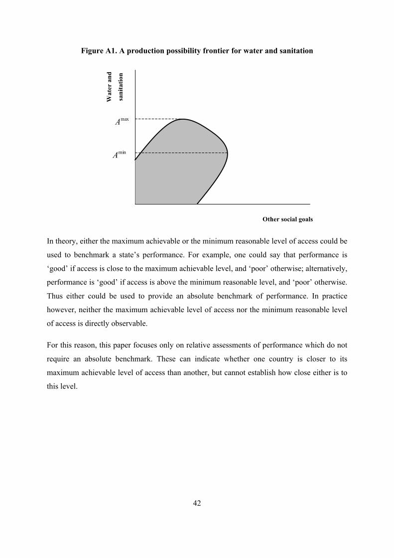
42

Figure A1. A production possibility frontier for water and sanitation

In theory, either the maximum achievable or the minimum reasonable level of access could be

used to benchmark a state’s performance. For example, one could say that performance is

‘good’ if access is close to the maximum achievable level, and ‘poor’ otherwise; alternatively,

performance is ‘good’ if access is above the minimum reasonable level, and ‘poor’ otherwise.

Thus either could be used to provide an absolute benchmark of performance. In practice

however, neither the maximum achievable level of access nor the minimum reasonable level

of access is directly observable.

For this reason, this paper focuses only on relative assessments of performance which do not

require an absolute benchmark. These can indicate whether one country is closer to its

maximum achievable level of access than another, but cannot establish how close either is to

this level.

Other social goals

maxA

minA

Wat

er a

nd

sani

tatio

n

d sa

nita

tion

sani

ot

sani

tatio

n

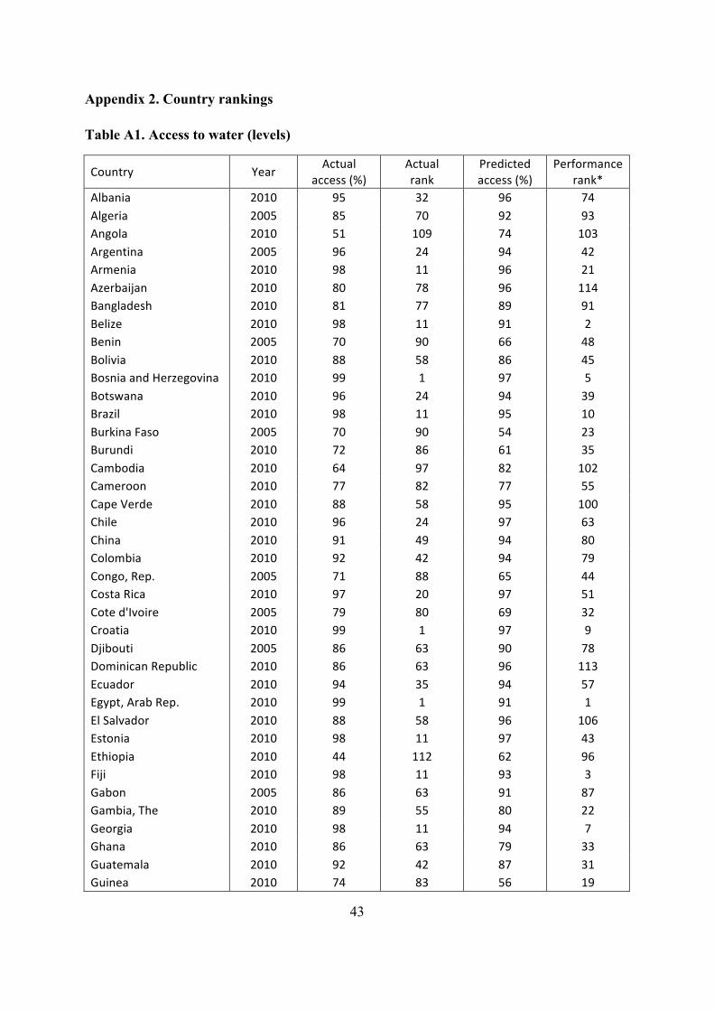
43

Appendix 2. Country rankings

Table A1. Access to water (levels)

Country   Year   Actual    access  (%)  

Actual    rank  

Predicted  access  (%)  

Performance  rank*  

Albania   2010   95   32   96   74  Algeria   2005   85   70   92   93  Angola   2010   51   109   74   103  Argentina   2005   96   24   94   42  Armenia   2010   98   11   96   21  Azerbaijan   2010   80   78   96   114  Bangladesh   2010   81   77   89   91  Belize   2010   98   11   91   2  Benin   2005   70   90   66   48  Bolivia   2010   88   58   86   45  Bosnia  and  Herzegovina   2010   99   1   97   5  Botswana   2010   96   24   94   39  Brazil   2010   98   11   95   10  Burkina  Faso   2005   70   90   54   23  Burundi   2010   72   86   61   35  Cambodia   2010   64   97   82   102  Cameroon   2010   77   82   77   55  Cape  Verde   2010   88   58   95   100  Chile   2010   96   24   97   63  China   2010   91   49   94   80  Colombia   2010   92   42   94   79  Congo,  Rep.   2005   71   88   65   44  Costa  Rica   2010   97   20   97   51  Cote  d'Ivoire   2005   79   80   69   32  Croatia   2010   99   1   97   9  Djibouti   2005   86   63   90   78  Dominican  Republic   2010   86   63   96   113  Ecuador   2010   94   35   94   57  Egypt,  Arab  Rep.   2010   99   1   91   1  El  Salvador   2010   88   58   96   106  Estonia   2010   98   11   97   43  Ethiopia   2010   44   112   62   96  Fiji   2010   98   11   93   3  Gabon   2005   86   63   91   87  Gambia,  The   2010   89   55   80   22  Georgia   2010   98   11   94   7  Ghana   2010   86   63   79   33  Guatemala   2010   92   42   87   31  Guinea   2010   74   83   56   19  

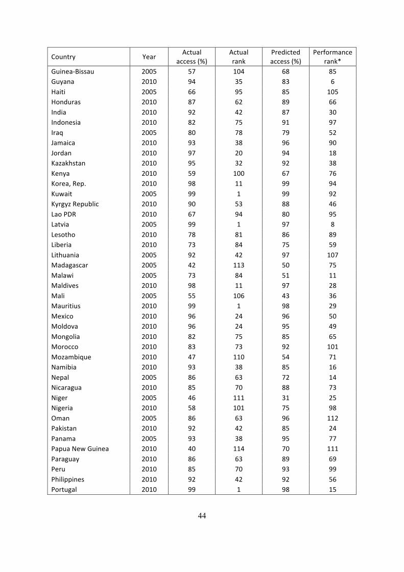
44

Country   Year   Actual    access  (%)  

Actual    rank  

Predicted  access  (%)  

Performance  rank*  

Guinea-­‐Bissau   2005   57   104   68   85  Guyana   2010   94   35   83   6  Haiti   2005   66   95   85   105  Honduras   2010   87   62   89   66  India   2010   92   42   87   30  Indonesia   2010   82   75   91   97  Iraq   2005   80   78   79   52  Jamaica   2010   93   38   96   90  Jordan   2010   97   20   94   18  Kazakhstan   2010   95   32   92   38  Kenya   2010   59   100   67   76  Korea,  Rep.   2010   98   11   99   94  Kuwait   2005   99   1   99   92  Kyrgyz  Republic   2010   90   53   88   46  Lao  PDR   2010   67   94   80   95  Latvia   2005   99   1   97   8  Lesotho   2010   78   81   86   89  Liberia   2010   73   84   75   59  Lithuania   2005   92   42   97   107  Madagascar   2005   42   113   50   75  Malawi   2005   73   84   51   11  Maldives   2010   98   11   97   28  Mali   2005   55   106   43   36  Mauritius   2010   99   1   98   29  Mexico   2010   96   24   96   50  Moldova   2010   96   24   95   49  Mongolia   2010   82   75   85   65  Morocco   2010   83   73   92   101  Mozambique   2010   47   110   54   71  Namibia   2010   93   38   85   16  Nepal   2005   86   63   72   14  Nicaragua   2010   85   70   88   73  Niger   2005   46   111   31   25  Nigeria   2010   58   101   75   98  Oman   2005   86   63   96   112  Pakistan   2010   92   42   85   24  Panama   2005   93   38   95   77  Papua  New  Guinea   2010   40   114   70   111  Paraguay   2010   86   63   89   69  Peru   2010   85   70   93   99  Philippines   2010   92   42   92   56  Portugal   2010   99   1   98   15  

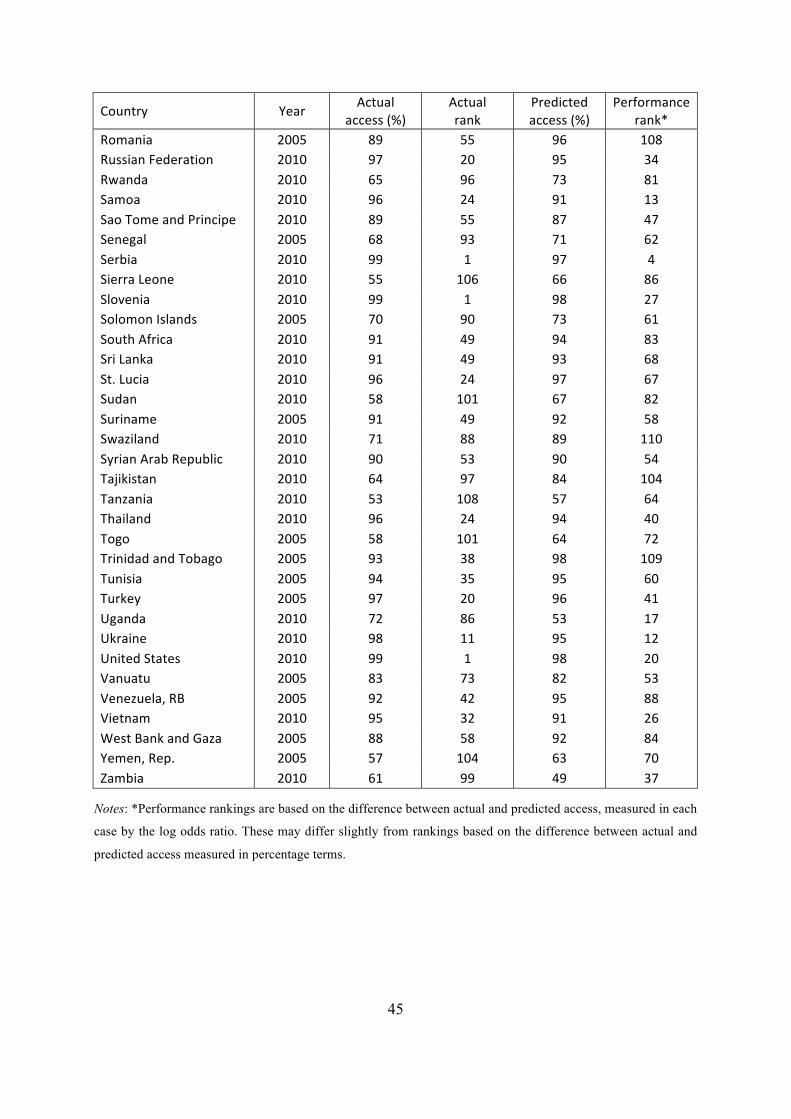
45

Country   Year   Actual    access  (%)  

Actual    rank  

Predicted  access  (%)  

Performance  rank*  

Romania   2005   89   55   96   108  Russian  Federation   2010   97   20   95   34  Rwanda   2010   65   96   73   81  Samoa   2010   96   24   91   13  Sao  Tome  and  Principe   2010   89   55   87   47  Senegal   2005   68   93   71   62  Serbia   2010   99   1   97   4  Sierra  Leone   2010   55   106   66   86  Slovenia   2010   99   1   98   27  Solomon  Islands   2005   70   90   73   61  South  Africa   2010   91   49   94   83  Sri  Lanka   2010   91   49   93   68  St.  Lucia   2010   96   24   97   67  Sudan   2010   58   101   67   82  Suriname   2005   91   49   92   58  Swaziland   2010   71   88   89   110  Syrian  Arab  Republic   2010   90   53   90   54  Tajikistan   2010   64   97   84   104  Tanzania   2010   53   108   57   64  Thailand   2010   96   24   94   40  Togo   2005   58   101   64   72  Trinidad  and  Tobago   2005   93   38   98   109  Tunisia   2005   94   35   95   60  Turkey   2005   97   20   96   41  Uganda   2010   72   86   53   17  Ukraine   2010   98   11   95   12  United  States   2010   99   1   98   20  Vanuatu   2005   83   73   82   53  Venezuela,  RB   2005   92   42   95   88  Vietnam   2010   95   32   91   26  West  Bank  and  Gaza   2005   88   58   92   84  Yemen,  Rep.   2005   57   104   63   70  Zambia   2010   61   99   49   37  

Notes: *Performance rankings are based on the difference between actual and predicted access, measured in each

case by the log odds ratio. These may differ slightly from rankings based on the difference between actual and

predicted access measured in percentage terms.

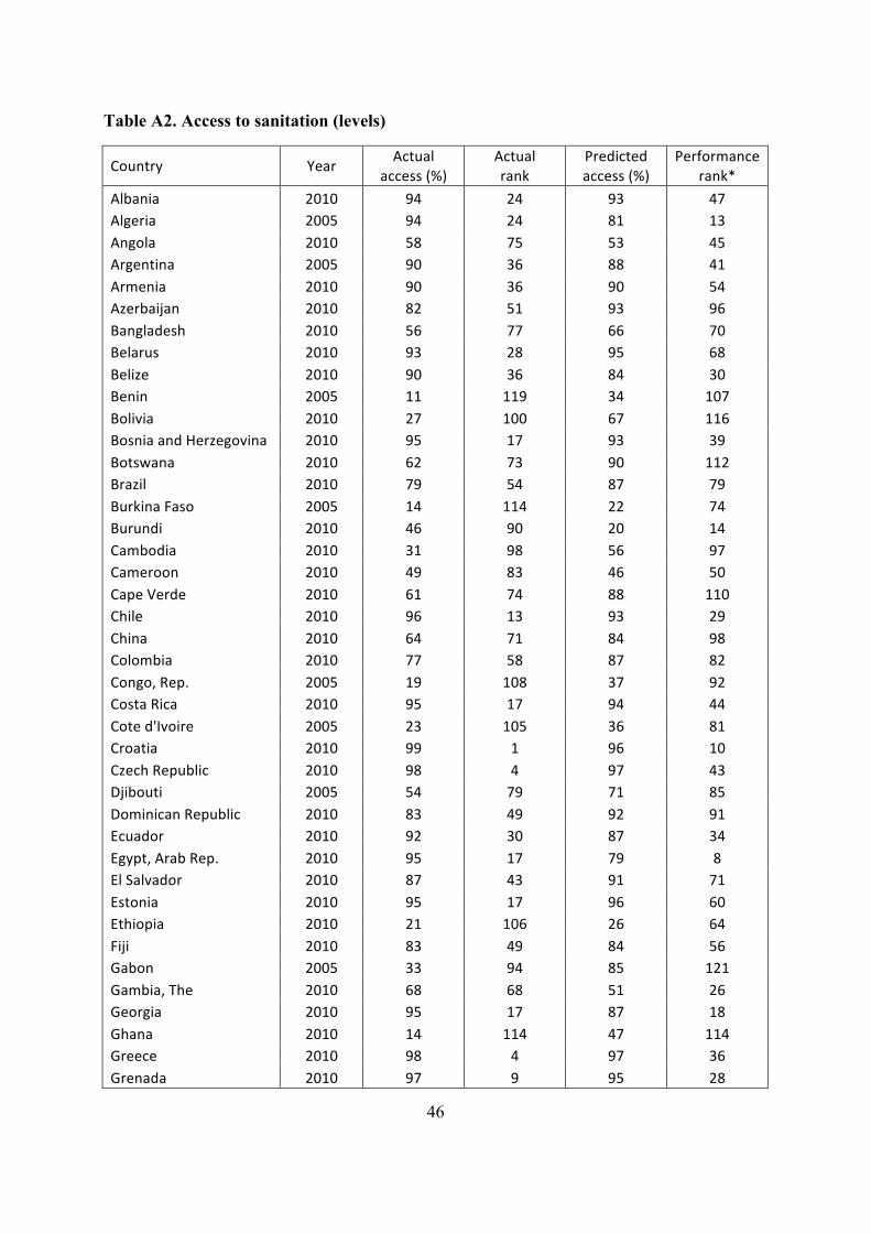
46

Table A2. Access to sanitation (levels)

Country   Year   Actual    access  (%)  

Actual    rank  

Predicted  access  (%)  

Performance  rank*  

Albania   2010   94   24   93   47  Algeria   2005   94   24   81   13  Angola   2010   58   75   53   45  Argentina   2005   90   36   88   41  Armenia   2010   90   36   90   54  Azerbaijan   2010   82   51   93   96  Bangladesh   2010   56   77   66   70  Belarus   2010   93   28   95   68  Belize   2010   90   36   84   30  Benin   2005   11   119   34   107  Bolivia   2010   27   100   67   116  Bosnia  and  Herzegovina   2010   95   17   93   39  Botswana   2010   62   73   90   112  Brazil   2010   79   54   87   79  Burkina  Faso   2005   14   114   22   74  Burundi   2010   46   90   20   14  Cambodia   2010   31   98   56   97  Cameroon   2010   49   83   46   50  Cape  Verde   2010   61   74   88   110  Chile   2010   96   13   93   29  China   2010   64   71   84   98  Colombia   2010   77   58   87   82  Congo,  Rep.   2005   19   108   37   92  Costa  Rica   2010   95   17   94   44  Cote  d'Ivoire   2005   23   105   36   81  Croatia   2010   99   1   96   10  Czech  Republic   2010   98   4   97   43  Djibouti   2005   54   79   71   85  Dominican  Republic   2010   83   49   92   91  Ecuador   2010   92   30   87   34  Egypt,  Arab  Rep.   2010   95   17   79   8  El  Salvador   2010   87   43   91   71  Estonia   2010   95   17   96   60  Ethiopia   2010   21   106   26   64  Fiji   2010   83   49   84   56  Gabon   2005   33   94   85   121  Gambia,  The   2010   68   68   51   26  Georgia   2010   95   17   87   18  Ghana   2010   14   114   47   114  Greece   2010   98   4   97   36  Grenada   2010   97   9   95   28  

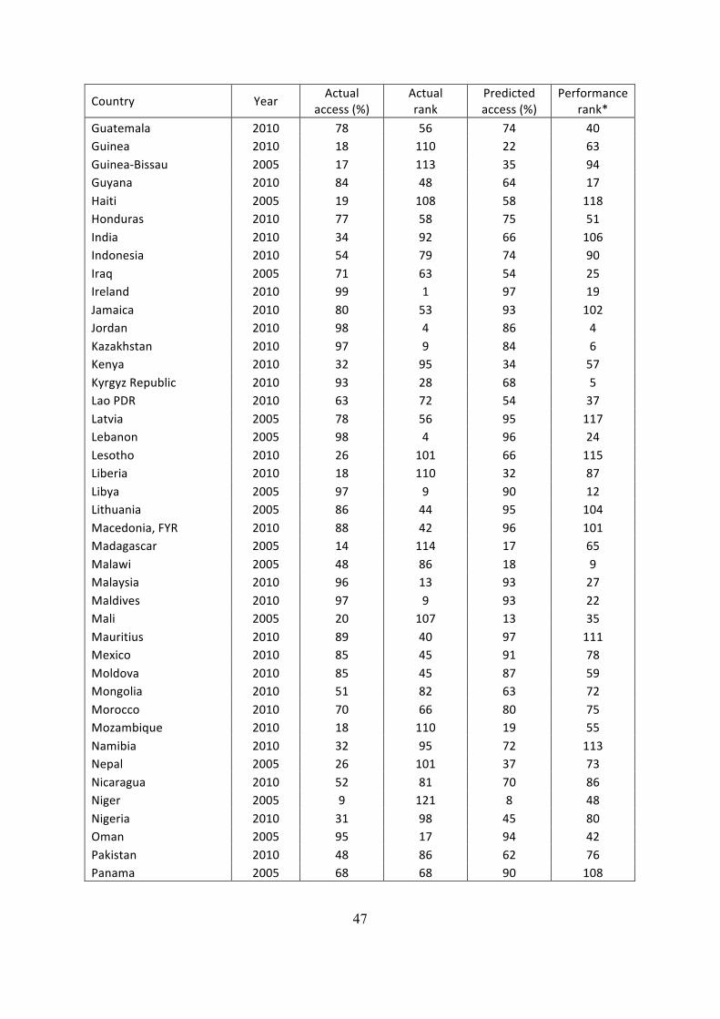
47

Country   Year   Actual    access  (%)  

Actual    rank  

Predicted  access  (%)  

Performance  rank*  

Guatemala   2010   78   56   74   40  Guinea   2010   18   110   22   63  Guinea-­‐Bissau   2005   17   113   35   94  Guyana   2010   84   48   64   17  Haiti   2005   19   108   58   118  Honduras   2010   77   58   75   51  India   2010   34   92   66   106  Indonesia   2010   54   79   74   90  Iraq   2005   71   63   54   25  Ireland   2010   99   1   97   19  Jamaica   2010   80   53   93   102  Jordan   2010   98   4   86   4  Kazakhstan   2010   97   9   84   6  Kenya   2010   32   95   34   57  Kyrgyz  Republic   2010   93   28   68   5  Lao  PDR   2010   63   72   54   37  Latvia   2005   78   56   95   117  Lebanon   2005   98   4   96   24  Lesotho   2010   26   101   66   115  Liberia   2010   18   110   32   87  Libya   2005   97   9   90   12  Lithuania   2005   86   44   95   104  Macedonia,  FYR   2010   88   42   96   101  Madagascar   2005   14   114   17   65  Malawi   2005   48   86   18   9  Malaysia   2010   96   13   93   27  Maldives   2010   97   9   93   22  Mali   2005   20   107   13   35  Mauritius   2010   89   40   97   111  Mexico   2010   85   45   91   78  Moldova   2010   85   45   87   59  Mongolia   2010   51   82   63   72  Morocco   2010   70   66   80   75  Mozambique   2010   18   110   19   55  Namibia   2010   32   95   72   113  Nepal   2005   26   101   37   73  Nicaragua   2010   52   81   70   86  Niger   2005   9   121   8   48  Nigeria   2010   31   98   45   80  Oman   2005   95   17   94   42  Pakistan   2010   48   86   62   76  Panama   2005   68   68   90   108  

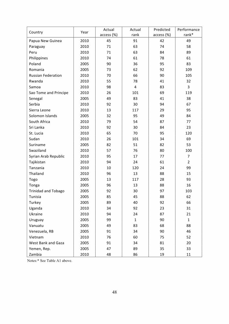
48

Country   Year   Actual    access  (%)  

Actual    rank  

Predicted  access  (%)  

Performance  rank*  

Papua  New  Guinea   2010   45   91   42   49  Paraguay   2010   71   63   74   58  Peru   2010   71   63   84   89  Philippines   2010   74   61   78   61  Poland   2005   90   36   95   83  Romania   2005   73   62   92   109  Russian  Federation   2010   70   66   90   105  Rwanda   2010   55   78   41   32  Samoa   2010   98   4   83   3  Sao  Tome  and  Principe   2010   26   101   69   119  Senegal   2005   49   83   41   38  Serbia   2010   92   30   94   67  Sierra  Leone   2010   13   117   29   95  Solomon  Islands   2005   32   95   49   84  South  Africa   2010   79   54   87   77  Sri  Lanka   2010   92   30   84   23  St.  Lucia   2010   65   70   95   120  Sudan   2010   26   101   34   69  Suriname   2005   82   51   82   53  Swaziland   2010   57   76   80   100  Syrian  Arab  Republic   2010   95   17   77   7  Tajikistan   2010   94   24   61   2  Tanzania   2010   10   120   24   99  Thailand   2010   96   13   88   15  Togo   2005   13   117   28   93  Tonga   2005   96   13   88   16  Trinidad  and  Tobago   2005   92   30   97   103  Tunisia   2005   85   45   88   62  Turkey   2005   89   40   92   66  Uganda   2010   34   92   23   31  Ukraine   2010   94   24   87   21  Uruguay   2005   99   1   90   1  Vanuatu   2005   49   83   68   88  Venezuela,  RB   2005   91   34   90   46  Vietnam   2010   76   60   75   52  West  Bank  and  Gaza   2005   91   34   81   20  Yemen,  Rep.   2005   47   89   35   33  Zambia   2010   48   86   19   11  

Notes:* See Table A1 above.

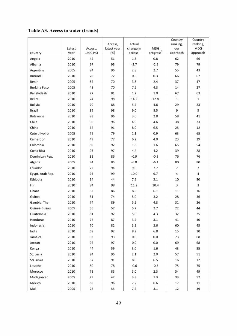
49

Table A3. Access to water (trends)

country  Latest  year  

Access,  1990  (%)  

Access,  latest  year  

(%)  

Actual  change  in  access1  

MDG  progress2  

Country  ranking,  our  

approach  

Country  ranking,  MDG  

approach  

Angola   2010   42   51   1.8   0.8   62   66  

Albania   2010   97   95   -­‐2.7   -­‐2.6   79   79  

Argentina   2005   94   96   2.8   2.7   55   43  

Burundi   2010   70   72   0.5   0.3   66   67  

Benin   2005   57   70   3.8   2.4   37   47  

Burkina  Faso   2005   43   70   7.5   4.3   14   27  

Bangladesh   2010   77   81   1.2   1.0   67   63  

Belize   2010   74   98   14.2   12.8   1   1  

Bolivia   2010   70   88   5.7   4.6   29   23  

Brazil   2010   89   98   9.0   8.5   9   5  

Botswana   2010   93   96   3.0   2.8   58   41  

Chile   2010   90   96   4.9   4.6   38   23  

China   2010   67   91   8.0   6.5   25   12  

Cote  d'Ivoire   2005   76   79   1.1   0.9   63   65  

Cameroon   2010   49   77   6.2   4.0   23   29  

Colombia   2010   89   92   1.8   1.6   65   54  

Costa  Rica   2010   93   97   4.4   4.2   39   28  

Dominican  Rep.   2010   88   86   -­‐0.9   -­‐0.8   76   76  

Algeria   2005   94   85   -­‐6.8   -­‐6.1   80   80  

Ecuador   2010   72   94   9.0   7.7   7   7  

Egypt,  Arab  Rep.   2010   93   99   10.0   9.7   4   4  

Ethiopia   2010   14   44   7.9   2.1   10   50  

Fiji   2010   84   98   11.2   10.4   3   3  

Ghana   2010   53   86   8.5   6.1   11   16  

Guinea   2010   51   74   5.0   3.2   28   36  

Gambia,  The   2010   74   89   5.2   4.3   31   26  

Guinea-­‐Bissau   2005   36   57   5.7   2.7   22   44  

Guatemala   2010   81   92   5.0   4.3   32   25  

Honduras   2010   76   87   3.7   3.1   41   40  

Indonesia   2010   70   82   3.3   2.6   60   45  

India   2010   69   92   8.2   6.8   15   10  

Jamaica   2010   93   93   0.0   0.0   73   68  

Jordan   2010   97   97   0.0   0.0   69   68  

Kenya   2010   44   59   3.0   1.6   43   55  

St.  Lucia   2010   94   96   2.1   2.0   57   51  

Sri  Lanka   2010   67   91   8.0   6.5   16   12  

Lesotho   2010   80   78   -­‐0.6   -­‐0.5   75   75  

Morocco   2010   73   83   3.0   2.3   54   49  

Madagascar   2005   29   42   3.8   1.3   33   57  

Mexico   2010   85   96   7.2   6.6   17   11  

Mali   2005   28   55   7.6   3.1   12   39  

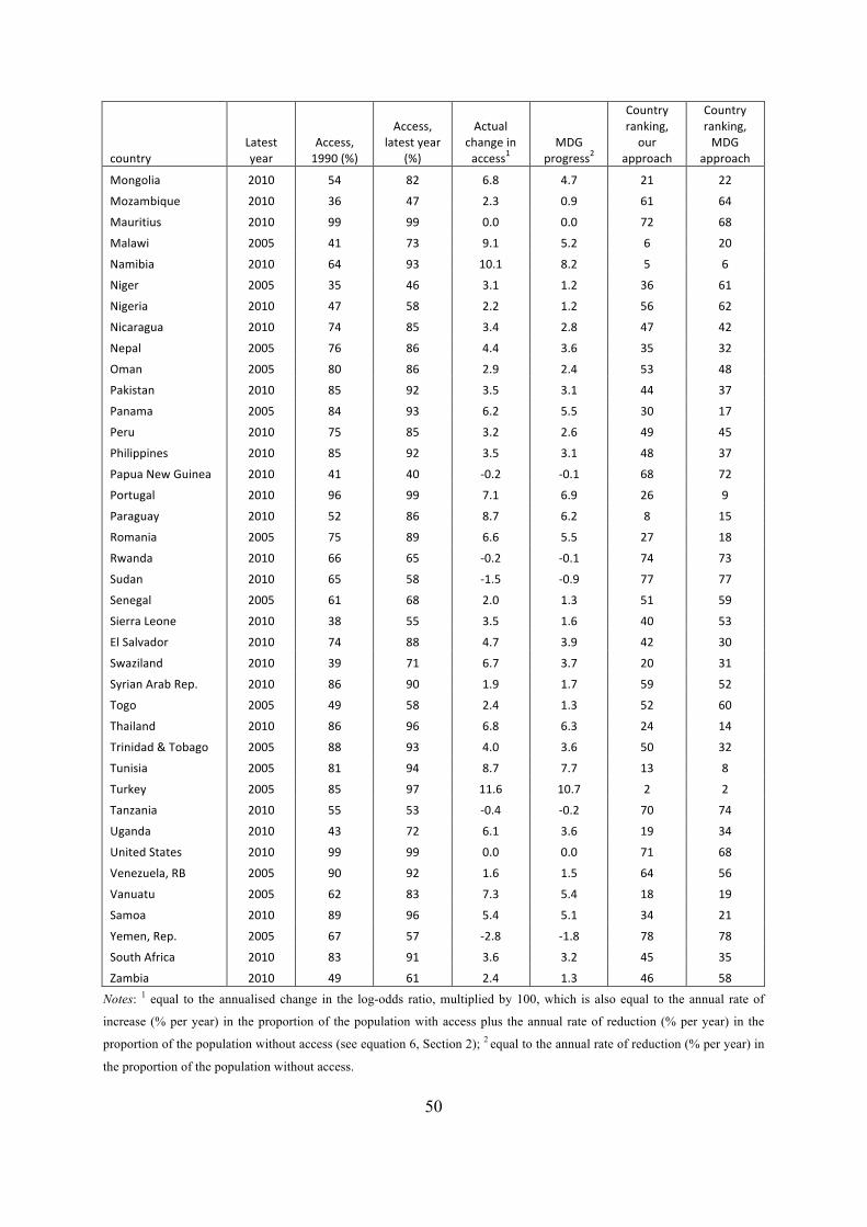
50

country  Latest  year  

Access,  1990  (%)  

Access,  latest  year  

(%)  

Actual  change  in  access1  

MDG  progress2  

Country  ranking,  our  

approach  

Country  ranking,  MDG  

approach  

Mongolia   2010   54   82   6.8   4.7   21   22  

Mozambique   2010   36   47   2.3   0.9   61   64  

Mauritius   2010   99   99   0.0   0.0   72   68  

Malawi   2005   41   73   9.1   5.2   6   20  

Namibia   2010   64   93   10.1   8.2   5   6  

Niger   2005   35   46   3.1   1.2   36   61  

Nigeria   2010   47   58   2.2   1.2   56   62  

Nicaragua   2010   74   85   3.4   2.8   47   42  

Nepal   2005   76   86   4.4   3.6   35   32  

Oman   2005   80   86   2.9   2.4   53   48  

Pakistan   2010   85   92   3.5   3.1   44   37  

Panama   2005   84   93   6.2   5.5   30   17  

Peru   2010   75   85   3.2   2.6   49   45  

Philippines   2010   85   92   3.5   3.1   48   37  

Papua  New  Guinea   2010   41   40   -­‐0.2   -­‐0.1   68   72  

Portugal   2010   96   99   7.1   6.9   26   9  

Paraguay   2010   52   86   8.7   6.2   8   15  

Romania   2005   75   89   6.6   5.5   27   18  

Rwanda   2010   66   65   -­‐0.2   -­‐0.1   74   73  

Sudan   2010   65   58   -­‐1.5   -­‐0.9   77   77  

Senegal   2005   61   68   2.0   1.3   51   59  

Sierra  Leone   2010   38   55   3.5   1.6   40   53  

El  Salvador   2010   74   88   4.7   3.9   42   30  

Swaziland   2010   39   71   6.7   3.7   20   31  

Syrian  Arab  Rep.   2010   86   90   1.9   1.7   59   52  

Togo   2005   49   58   2.4   1.3   52   60  

Thailand   2010   86   96   6.8   6.3   24   14  

Trinidad  &  Tobago   2005   88   93   4.0   3.6   50   32  

Tunisia   2005   81   94   8.7   7.7   13   8  

Turkey   2005   85   97   11.6   10.7   2   2  

Tanzania   2010   55   53   -­‐0.4   -­‐0.2   70   74  

Uganda   2010   43   72   6.1   3.6   19   34  

United  States   2010   99   99   0.0   0.0   71   68  

Venezuela,  RB   2005   90   92   1.6   1.5   64   56  

Vanuatu   2005   62   83   7.3   5.4   18   19  

Samoa   2010   89   96   5.4   5.1   34   21  

Yemen,  Rep.   2005   67   57   -­‐2.8   -­‐1.8   78   78  

South  Africa   2010   83   91   3.6   3.2   45   35  

Zambia   2010   49   61   2.4   1.3   46   58  

Notes: 1 equal to the annualised change in the log-odds ratio, multiplied by 100, which is also equal to the annual rate of

increase (% per year) in the proportion of the population with access plus the annual rate of reduction (% per year) in the

proportion of the population without access (see equation 6, Section 2); 2 equal to the annual rate of reduction (% per year) in

the proportion of the population without access.

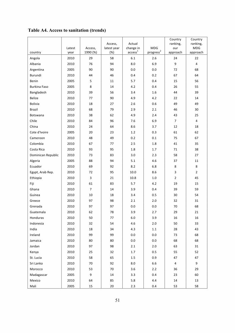
51

Table A4. Access to sanitation (trends)

country  Latest  year  

Access,  1990  (%)  

Access,  latest  year  

(%)  

Actual  change  in  access1  

MDG  progress2  

Country  ranking,  our  

approach  

Country  ranking,  MDG  

approach  

Angola   2010   29   58   6.1   2.6   24   22  

Albania   2010   76   94   8.0   6.9   9   4  

Argentina   2005   90   90   0.0   0.0   72   68  

Burundi   2010   44   46   0.4   0.2   67   64  

Benin   2005   5   11   5.7   0.4   15   56  

Burkina  Faso   2005   8   14   4.2   0.4   26   55  

Bangladesh   2010   39   56   3.4   1.6   44   39  

Belize   2010   77   90   4.9   4.2   22   14  

Bolivia   2010   18   27   2.6   0.6   49   49  

Brazil   2010   68   79   2.9   2.1   46   30  

Botswana   2010   38   62   4.9   2.4   43   25  

Chile   2010   84   96   7.6   6.9   7   4  

China   2010   24   64   8.6   3.7   12   18  

Cote  d'Ivoire   2005   20   23   1.2   0.3   61   62  

Cameroon   2010   48   49   0.2   0.1   75   67  

Colombia   2010   67   77   2.5   1.8   41   35  

Costa  Rica   2010   93   95   1.8   1.7   71   38  

Dominican  Republic   2010   73   83   3.0   2.3   58   27  

Algeria   2005   88   94   5.1   4.6   37   11  

Ecuador   2010   69   92   8.2   6.8   8   8  

Egypt,  Arab  Rep.   2010   72   95   10.0   8.6   3   2  

Ethiopia   2010   3   21   10.8   1.0   2   45  

Fiji   2010   61   83   5.7   4.2   19   15  

Ghana   2010   7   14   3.9   0.4   39   59  

Guinea   2010   10   18   3.4   0.5   30   54  

Greece   2010   97   98   2.1   2.0   32   31  

Grenada   2010   97   97   0.0   0.0   70   68  

Guatemala   2010   62   78   3.9   2.7   29   21  

Honduras   2010   50   77   6.0   3.9   16   16  

Indonesia   2010   32   54   4.6   2.0   50   33  

India   2010   18   34   4.3   1.1   28   43  

Ireland   2010   99   99   0.0   0.0   73   68  

Jamaica   2010   80   80   0.0   0.0   68   68  

Jordan   2010   97   98   2.1   2.0   63   31  

Kenya   2010   25   32   1.7   0.5   55   52  

St.  Lucia   2010   58   65   1.5   0.9   47   47  

Sri  Lanka   2010   70   92   8.0   6.6   4   9  

Morocco   2010   53   70   3.6   2.2   36   29  

Madagascar   2005   9   14   3.3   0.4   23   60  

Mexico   2010   64   85   5.8   4.4   14   13  

Mali   2005   15   20   2.3   0.4   53   58  

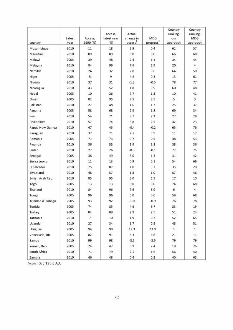
52

country  Latest  year  

Access,  1990  (%)  

Access,  latest  year  

(%)  

Actual  change  in  access1  

MDG  progress2  

Country  ranking,  our  

approach  

Country  ranking,  MDG  

approach  

Mozambique   2010   11   18   2.9   0.4   62   57  

Mauritius   2010   89   89   0.0   0.0   66   68  

Malawi   2005   39   48   2.4   1.1   34   44  

Malaysia   2010   84   96   7.6   6.9   20   4  

Namibia   2010   24   32   2.0   0.6   64   50  

Niger   2005   5   9   4.2   0.3   13   61  

Nigeria   2010   37   31   -­‐1.3   -­‐0.5   78   77  

Nicaragua   2010   43   52   1.8   0.9   60   48  

Nepal   2005   10   26   7.7   1.3   10   41  

Oman   2005   82   95   9.5   8.5   5   3  

Pakistan   2010   27   48   4.6   1.7   25   37  

Panama   2005   58   68   2.9   1.8   69   34  

Peru   2010   54   71   3.7   2.3   27   28  

Philippines   2010   57   74   3.8   2.5   42   23  

Papua  New  Guinea   2010   47   45   -­‐0.4   -­‐0.2   65   76  

Paraguay   2010   37   71   7.1   3.9   11   17  

Romania   2005   71   73   0.7   0.5   48   53  

Rwanda   2010   36   55   3.9   1.8   38   36  

Sudan   2010   27   26   -­‐0.3   -­‐0.1   77   75  

Senegal   2005   38   49   3.0   1.3   31   42  

Sierra  Leone   2010   11   13   0.9   0.1   54   66  

El  Salvador   2010   75   87   4.0   3.3   35   20  

Swaziland   2010   48   57   1.8   1.0   57   46  

Syrian  Arab  Rep.   2010   85   95   6.0   5.5   17   10  

Togo   2005   13   13   0.0   0.0   74   68  

Thailand   2010   84   96   7.6   6.9   6   4  

Tonga   2005   96   96   0.0   0.0   59   68  

Trinidad  &  Tobago   2005   93   92   -­‐1.0   -­‐0.9   76   78  

Tunisia   2005   74   85   4.6   3.7   33   19  

Turkey   2005   84   89   2.9   2.5   51   24  

Tanzania   2010   7   10   1.9   0.2   52   65  

Uganda   2010   27   34   1.7   0.5   45   51  

Uruguay   2005   94   99   12.3   11.9   1   1  

Venezuela,  RB   2005   82   91   5.3   4.6   21   11  

Samoa   2010   99   98   -­‐3.5   -­‐3.5   79   79  

Yemen,  Rep.   2005   24   47   6.9   2.4   18   26  

South  Africa   2010   71   79   2.1   1.6   56   40  

Zambia   2010   46   48   0.4   0.2   40   63  

Notes: See Table A3.