A DYNAMIC MODEL OF FOOD AND CLEAN ENERGY

by

Ujjayant Chakravorty1, Bertrand Magné2 and Michel Moreaux3

Abstract

In the midwestern United States, ethanol produced from corn is mixed with gasoline to meet

clean air standards. Allocating land to produce clean fuel means taking away land from farming.

We examine a model in which a scarce fossil fuel (e.g., oil) causes pollution but may be

substituted by a clean fuel produced from land. Methodologically, we extend the Hotelling model

to consider a substitute produced in the agricultural sector. We discover a range of prices within

which the land-based fuel may substitute for the fossil fuel. When land is abundant, the supply of

the clean fuel may exhibit multiple discontinuities. Environmental regulation may cause food

production and farm prices to remain constant for a period of time.

JEL classification: Q41, Q42, Q15

Keywords: Agriculture, Environmental regulation, Hotelling theory, Land use, Pollution

1 Corresponding Author: Department of Economics, University of Central Florida, Orlando, FL 32816,USA and University of Toulouse, phone: 407 823 4728, fax 407 823 3269, uchakravorty@bus.ucf.edu. 2 University of Toulouse I (CEA, LERNA), 21 Allée de Brienne, 31000 Toulouse, France; 3 University of Toulouse I (IUF, IDEI and LERNA), 21 Allée de Brienne, 31000 Toulouse, France.

2

1. Introduction

The Ford Motor Company has introduced several types of Flexible Fuel Vehicles (FFVs) that run

on E85, a mixture of 85% ethanol (made from corn) and 15% gasoline. There are 3.5 million

FFVs already plying on US highways but only 400 fuelling stations that supply E85. A bill

passed by the US Senate provides tax credits for building E85 fueling stations. After the bill’s

passage, United States Sen. Barrack Obama said: “a fuel made of 85 percent Midwestern corn is

a lot more desirable than one made from 100 percent Middle Eastern Oil.”

The US Environmental Protection Agency is considering regulating a renewable energy standard,

by which a designated fraction of all gasoline must come from renewable energy sources such as

ethanol. These trends towards meeting clean energy goals through fuels produced from land

imply an increased competition for scarce land resources, especially in agriculture. Policy makers

in the US Midwest, for example are already worried about the effect of rising ethanol

consumption for energy on food prices (The New York Times, 2006).4

In this paper, we develop a dynamic model that examines this trade-off between producing clean

energy and using land for food production. The clean energy substitutes for a polluting non-

renewable resource such as oil. We derive an equivalence between Ricardian land rent and the

Hotelling rent for the nonrenewable resource. We show that the price of the clean fuel produced

from land must lie within precise bounds dictated by the amount of available land and the

demands for food and energy. These bounds determine the trigger price at which the land fuel is

used for energy and the price at which the nonrenewable resource is completely exhausted.

Supply of the land based fuel may occur in a discontinuous fashion when land is relatively

abundant. Ricardian rents to land as well as Hotelling rents to oil may increase over time.

We examine how environmental regulation imposed in the form of a limit on the stock of

pollution may affect the substitution to a land-based fuel. Unlike abatement technologies which

4 “High oil prices are dragging corn prices up with them, as the value of ethanol is pushed up by the value of the fuel it replaces,” The New York Times (2006).

3

may be used only when regulation is binding, the land-based fuel may be deployed before the

pollution stock is binding or later in time when pollution is no longer an issue.

There is a large literature on nonrenewable resources and pollution, including Forster (1980),

Sinclair (1994), Ulph and Ulph (1994), Farzin (1996), Hoel and Kverndokk (1996), Tahvonen

(1997) and Toman and Withagen (2000). The focus of these studies has largely been on the time

path of pollution and carbon taxes. Hoel (1984) examines a model in which a nonrenewable

resource has a perfect substitute in some of its uses but no substitute in others. He notes that

resource prices may jump at the time when the substitute production comes into play. The focus

of his paper is on market structure and price discrimination, not on the relationship between land

and energy use. Chakravorty, Magne and Moreaux (2006) extend a Hotelling model to explore

the allocation of a polluting nonrenewable resource and a clean backstop. This paper is an

extension of their approach, in which we explicitly model land allocation in an agricultural sector

that may produce both food and clean energy. The land endowment and magnitude of demands

for food and energy affect substitution between the fossil fuel and the land fuel. On the other

hand, pollution regulation in the energy sector affects the allocation of land in food production. In

general, the main contribution of this paper in the literature following Hotelling (1931) is in

explicitly linking the use of a nonrenewable resource over time to the allocation of land.

Section 2 outlines the basic dynamic model with land. In section 3 we develop intuition by

examining polar cases of the model in which land is allocated for food alone, for both food and

fuel after oil is completely depleted, and finally when both food and both sources of energy are

produced. In section 4, we integrate this land market equilibrium with the dynamic equilibrium in

the oil market. In section 5, we impose environmental regulation and consider when costly

pollution control technologies may be deployed. Section 6 concludes the paper.

2. The Model

We consider an economy in which utility U at any given time t is produced from food and

energy, denoted respectively byfq and eq .5 Utility is additive and given by the sub-utility

5 In order to prevent notational clutter, we avoid writing the time argument explicitly wherever possible.

4

functions ef uuU += . We further assume that { } RR:e,fi,ui →∈ + is of class 2C , strictly

increasing and strictly concave, satisfying the Inada conditions +∞=′+∞↓ )( lim iiq

qui

, where

i

iii dq

du)q(u =′ . Under these assumptions, the second derivative

2i

i2

ii dq

ud)q(u ≡′′ is negative. Denote

by pi the marginal surplus function and by di its inverse, i.e., )p(u)q(p)p(d i'1

i1

iii−− ≡≡ .

There are two primary factors, land and a fossil fuel which we call oil. Land is assumed to be

homogenous in quality, and its endowment is denoted byL . It can be used to produce food or an

energy crop such as corn that when converted to ethanol, serves as a clean substitute for oil.6

Let { }y,fi,Li ∈ , be the portion of land dedicated to producing food and energy, respectively.

Then the residual land 0LLL yf ≥−− is fallow. Denote byf andy the yield of food and the

land-based fuel per unit land which is assumed fixed. Their production at any instant of time is

given by fLf)t(f = and yLy)t(y = . The cost of inputs per unit land area is denoted

by { }y,fi,ci ∈ . These costs may include the cost of conversion of grain to ethanol. We assume

that they do not vary with the volume of food or land fuel produced. The average cost per unit

output is then given by fc f / and ycy / respectively. These commodities are not storable,

except at a prohibitive cost.

Energy can also be produced by using oil. Let )0(X be its initial stock, )t(X the residual stock at

time t and )t(x its rate of consumption so that )t(x)t(X −=•. Let xc be its average cost7 assumed

to be constant and lower than the unit cost of the land fuel, ycc yx /< . The land fuel and fossil

fuel are assumed to be perfect substitutes in final demand so that the total consumption of energy

at time t is equal to the sum of their extraction rates: )t(x)t(y)t(qe += .8 The land fuel is costly

6 The model may need to be significantly modified to consider energy sources such as wood from tree production because harvests tend to be discrete in time. 7 including the cost of extraction, processing and delivery. 8 Strictly speaking, this is not an accurate depiction of E85. That would imply strict complementarity of both fuels in clean energy production, so that ethanol and oil will be produced in fixed proportions. That is, oil will be directly used in the production both fossil and clean energy. As will be clear later, such an extension will make the model complicated but may not yield many fresh insights. Both oil and ethanol production must go down over time at

5

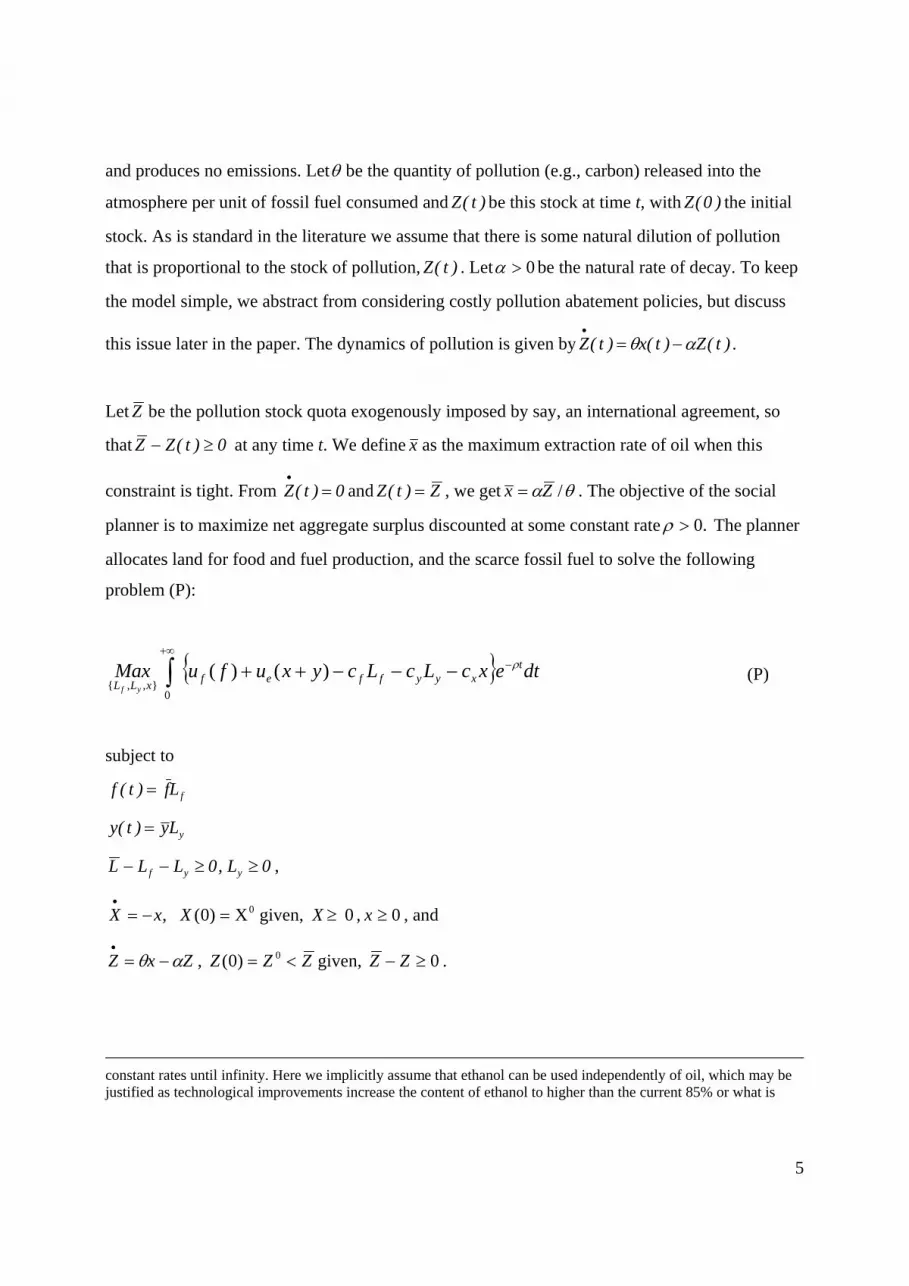
and produces no emissions. Letθ be the quantity of pollution (e.g., carbon) released into the

atmosphere per unit of fossil fuel consumed and)t(Z be this stock at time t, with )0(Z the initial

stock. As is standard in the literature we assume that there is some natural dilution of pollution

that is proportional to the stock of pollution, )t(Z . Let 0>α be the natural rate of decay. To keep

the model simple, we abstract from considering costly pollution abatement policies, but discuss

this issue later in the paper. The dynamics of pollution is given by )t(Z)t(x)t(Z αθ −=•.

LetZ be the pollution stock quota exogenously imposed by say, an international agreement, so

that 0)t(ZZ ≥− at any time t. We definex as the maximum extraction rate of oil when this

constraint is tight. From 0)t(Z =•and Z)t(Z = , we get θα /Zx = . The objective of the social

planner is to maximize net aggregate surplus discounted at some constant rate.0>ρ The planner

allocates land for food and fuel production, and the scarce fossil fuel to solve the following

problem (P):

{ } dtexcLcLcyxufuMax txyyffef

xLL yf

ρ−+∞ −−−++∫ )()(0

},,{ (P)

subject to

fLf)t(f =

yLy)t(y =

,0LLL yf ≥−− 0Ly ≥ ,

0 given, X)0( , 0 ≥=−=•XXxX , 0≥x , and

0 given, )0( , 0 ≥−<=−=•ZZZZZZxZ αθ .

constant rates until infinity. Here we implicitly assume that ethanol can be used independently of oil, which may be justified as technological improvements increase the content of ethanol to higher than the current 85% or what is

6

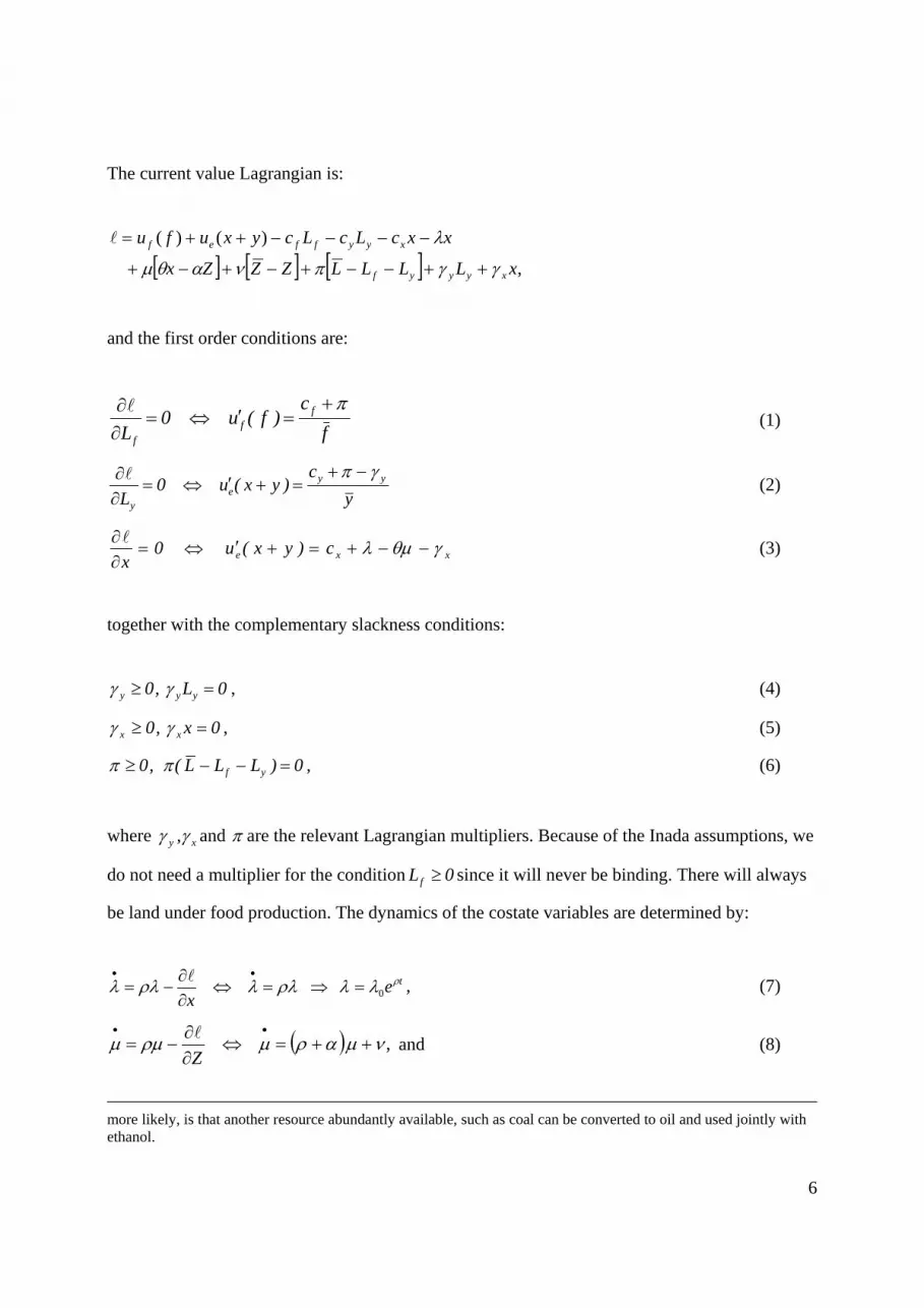
The current value Lagrangian is:

[ ] [ ] [ ] ,

)()(

xLLLLZZZx

xxcLcLcyxufu

xyyyf

xyyffef

γγπναθµλ

++−−+−+−+−−−−++=l

and the first order conditions are:

f

c)f(u 0

Lf

ff

π+=′⇔=∂∂l

(1)

y

c)yx(u 0

Lyy

ey

γπ −+=+′⇔=∂∂l

(2)

xxe c)yx(u 0x

γθµλ −−+=+′⇔=∂∂l

(3)

together with the complementary slackness conditions:

0L ,0 yyy =≥ γγ , (4)

0x ,0 xx =≥ γγ , (5)

0)LLL(,0 yf =−−≥ ππ , (6)

where xy ,γγ and π are the relevant Lagrangian multipliers. Because of the Inada assumptions, we

do not need a multiplier for the condition 0L f ≥ since it will never be binding. There will always

be land under food production. The dynamics of the costate variables are determined by:

tex

ρλλρλλρλλ 0 =⇒=⇔∂∂−= •• l

, (7)

( ) , νµαρµρµµ ++=⇔∂∂−= ••Z

l and (8)

more likely, is that another resource abundantly available, such as coal can be converted to oil and used jointly with ethanol.

7

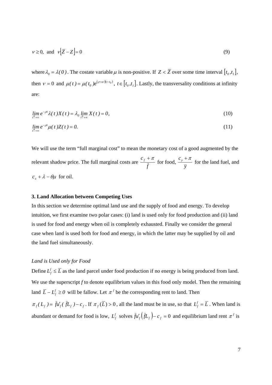
[ ] 0 and ,0 =−≥ ZZνν (9)

where )0(0 λλ = . The costate variableµ is non-positive. If ZZ < over some time interval [ ]10 t,t ,

then 0=ν and ( )( )0tt0 e)t()t( −+= αρµµ , [ ]10 t,tt∈ . Lastly, the transversality conditions at infinity

are:

,0)t(Xlim)t(X)t(elimt

0t

t== +∞↑

−+∞↑ λλρ (10)

.0)t(Z)t(elim t

t=−

+∞↑ µρ (11)

We will use the term “full marginal cost” to mean the monetary cost of a good augmented by the

relevant shadow price. The full marginal costs are f

c f π+ for food,

y

cy π+ for the land fuel, and

θµλ −+xc for oil.

3. Land Allocation between Competing Uses

In this section we determine optimal land use and the supply of food and energy. To develop

intuition, we first examine two polar cases: (i) land is used only for food production and (ii) land

is used for food and energy when oil is completely exhausted. Finally we consider the general

case when land is used both for food and energy, in which the latter may be supplied by oil and

the land fuel simultaneously.

Land is Used only for Food

Define LLff ≤ as the land parcel under food production if no energy is being produced from land.

We use the superscript f to denote equilibrium values in this food only model. Then the remaining

land 0LL ff ≥− will be fallow. Let fπ be the corresponding rent to land. Then

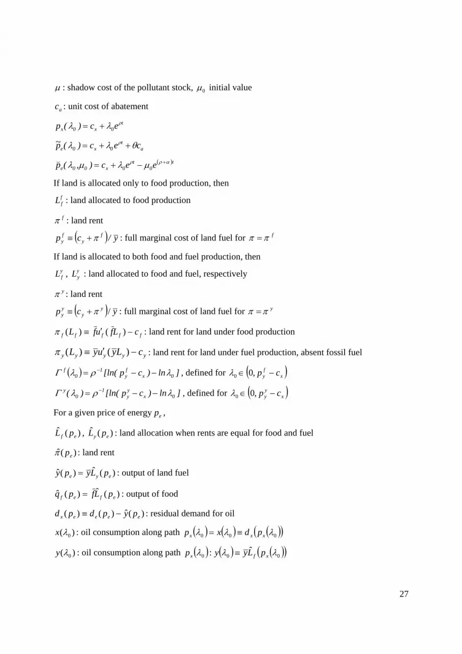
fffff c)Lf(uf)L( −′=π . If 0)( >Lfπ , all the land must be in use, so that LLff = . When land is

abundant or demand for food is low, ffL solves ( ) 0=−′ fff cLfuf and equilibrium land rent fπ is

8

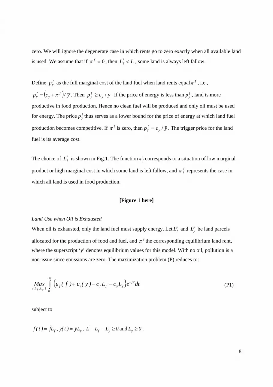
zero. We will ignore the degenerate case in which rents go to zero exactly when all available land

is used. We assume that if 0=fπ , then LLff < , some land is always left fallow.

Define fyp as the full marginal cost of the land fuel when land rents equalfπ , i.e.,

( ) y/cp fy

fy π+≡ . Then ycp y

fy /≥ . If the price of energy is less thanfyp , land is more

productive in food production. Hence no clean fuel will be produced and only oil must be used

for energy. The price fyp thus serves as a lower bound for the price of energy at which land fuel

production becomes competitive. If fπ is zero, then ycp yfy /= . The trigger price for the land

fuel is its average cost.

The choice of ffL is shown in Fig.1. The function1

fπ corresponds to a situation of low marginal

product or high marginal cost in which some land is left fallow, and 2fπ represents the case in

which all land is used in food production.

[Figure 1 here]

Land Use when Oil is Exhausted

When oil is exhausted, only the land fuel must supply energy. LetyfL and y

yL be land parcels

allocated for the production of food and fuel, and yπ the corresponding equilibrium land rent,

where the superscript ‘y’ denotes equilibrium values for this model. With no oil, pollution is a

non-issue since emissions are zero. The maximization problem (P) reduces to:

{ } dteLcLc)y(u)f(uMax tyyffef

0}L,L{ yf

ρ−+∞ −−+∫ (P1)

subject to

fLf)t(f = , yLy)t(y = , 0LLL yf ≥−− and 0Ly ≥ .

9

The necessary and the complementary slackness conditions are:

π+=′ ff c)f(uf ,

yye cyu γπ −+=′ )(y ,

0≥π and ,0)LLL( yf =−−π 0≥yγ and 0=yyLγ .

With no stock dynamics, (P1) is a static problem. Under the Inada conditions, 0Lyf > and when

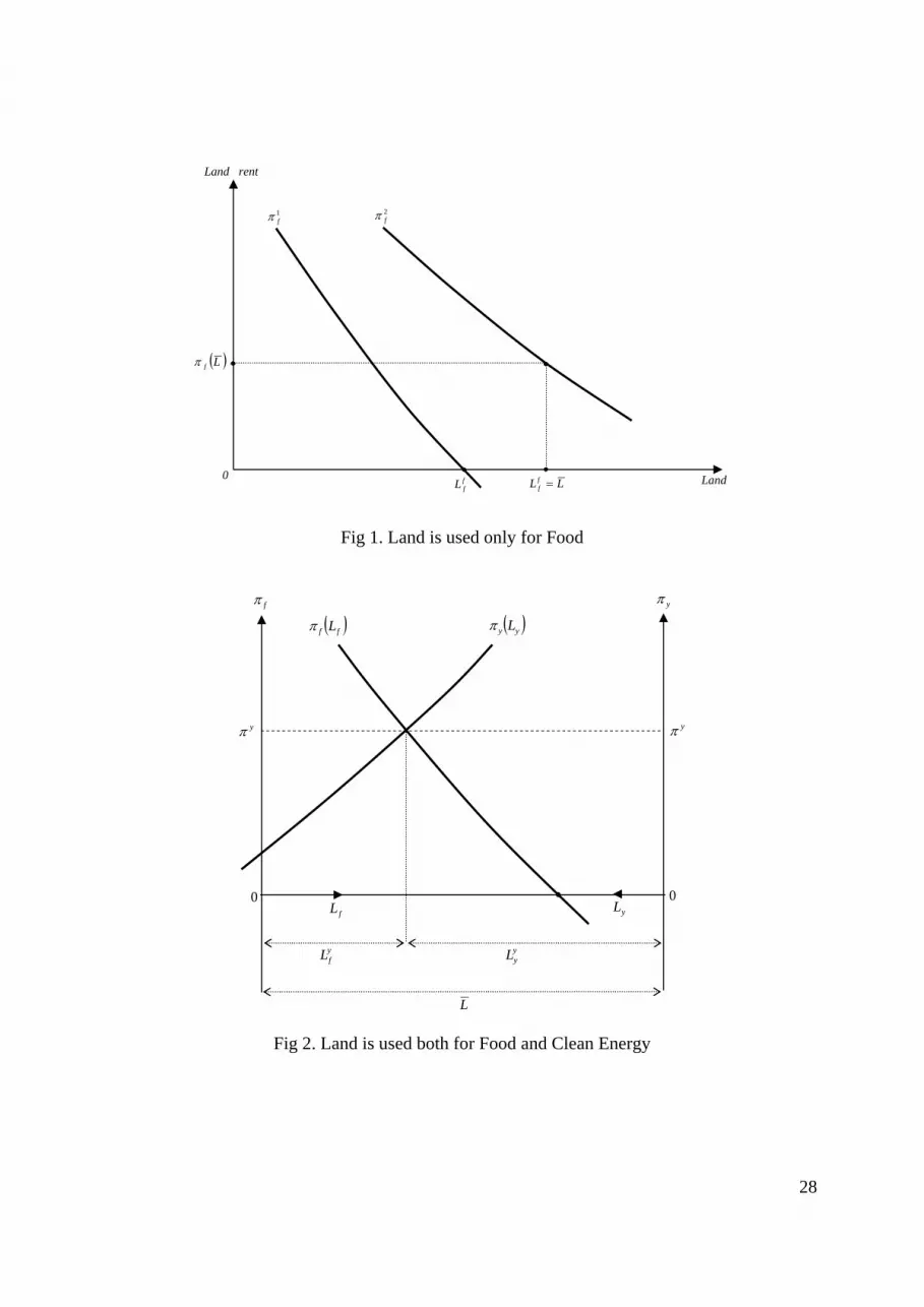
oil is exhausted, the land fuel must supply energy so that0Lyy > and 0=yγ . Let )( yy Lπ be the

rent to land allocated for land fuel production, i.e. yyyyy cLyuyL −′= )()(π . All the available

land will be used for food and energy production if equilibrium land rents are equal and strictly

positive, i.e., ( ) ( ) 0LLL fyff >−= ππ . This is shown in Fig. 2, in which the equilibrium rentyπ is

strictly positive. When land is abundant or demands are small, each marginal product may be

zero, i.e., yfL solves 0)L( ff =π and f

fyf LL = . In this case land allocated for food is exactly the

same as in the previous model with no energy production, andyyL solves 0)( =yy Lπ , with

LLL yy

yf <+ and the common land rent 0y =π . Some land is left fallow. If equilibrium land rents

are zero in the model with the land fuel, it can not be strictly positive in the food only case when

there is no competition for land. That is, we can not have 0y =π and 0>fπ .

[Figure 2 here]

Land Use for Food and Energy when Oil is Available

We now consider land allocation when oil is still available. Define yyp as the full marginal cost of

the clean fuel when the land rent is equal toyπ , i.e., y

cp

yyy

y

π+≡ . Rents must be higher in the

presence of competing uses, hence fy ππ ≥ . This implies that y

cpp yf

yyy ≥≥ . We then have

10

y

cp yf

y > if 0>fπ and fy

yy pp > if fy ππ > . We will see below that the price of energy is at

most equal to yyp , the highest price reached once oil is exhausted. If rents are zero both in the

food only and food and land fuel only models, 0fy == ππ , then some land must be fallow, i.e.,

LLL yf

yy <+ .9 In the food only model, there is no competition for land, hence rents will achieve

some lower bound, while in the model with no oil, all energy must come from the land fuel,

hence rents achieve some upper bound.

Consider energy supply for given energy prices yye pp ≤ . Define )(ˆ epπ as the land rent for which

the full marginal cost of the land fuel is equal to the price of energyep . This price must be at

least equal to the unit cost of the land fuel, ycy :

⎪⎩⎪⎨⎧ ≤<−

≤= yyeyye

ye

e ppyccpy

ycpp

,

,0)(π

Below we examine three possible cases: 0>fπ ; 0=fπ and 0>yπ and finally, 0== yf ππ .

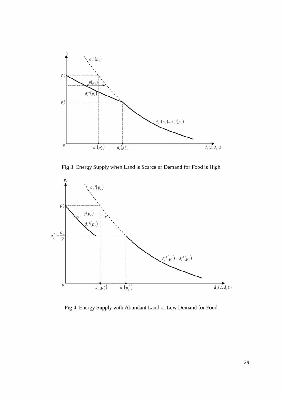
(a) All Available Land is Used under Food Production, 0>fπ :

When 0>fπ , the demand for food is high or the endowment of land is low. Then

yy

fyy ppyc ≤< . For energy prices f

ye pp < , we have fep ππ <)(ˆ . Since the rent under food

production is higher than in fuel production, all the available land must be used to grow food and

there will be no land fuel supplied to augment the use of oil. For higher energy

prices [ ]yy

fye ppp ,∈ , we have f

ep ππ >)(ˆ . The land fuel is competitive in the allocation of land,

hence 0>y and 0=yγ . Equalisation of land rents implies

yeffp cpycLfufe

−=−′ )( (12)

9 We neglect the degenerate case when 0fy == ππ and LLL y

fyy =+ .

11

so that

0)(²<′′=

fe

f

Lfuf

y

dp

dL. (13)

A higher price of energy induces a decrease in the land allocated to food and because

fy LLL −= , an increase in the land allocated to fuel. Let )(ˆef pL be the solution to (12) for [ ]y

yfye ppp ,∈ and equal zero for f

ye pp ≤ . Then the supply of landfuel as a function of ep given

by )(ˆ epy , is

[ ])p(LLy)p(y efe −= . (14)

Let the portion of energy supplied by oil be denoted by )( ex pd . It must equal the aggregate

demand for energy net the quantity supplied by the land fuel, )(ˆ)( eee pypd − . To see that

0)( ≥ex pd , note that because 0>fπ , when fye pp = , we have 0)( >f

yx pd and 0)(ˆ =fypy and

when yye pp = , )(ˆ)( y

yyye pypd = . Since )( ee pd is decreasing while )(ˆ epy is increasing we

conclude that 0)( ≥ex pd and )( ex pd must be decreasing from )( fye pd at f

ye pp = down to zero

at yye pp = . Furthermore )( ex pd is continuous at f

ye pp = although nondifferentiable. The

derived demand function for oil, )( ex pd is illustrated in Fig. 3

[Figure 3 here]

(b) Land is Fallow under Food Production but not for both Food and Energy, 0=fπ , 0>yπ :

This case may arise if there is enough land for food production but not for producing both food

and energy. Or if the demand for food is low relative to the demand for energy. The land rent

under food production is zero, but not when both food and energy are being produced after the

exhaustion of oil. Then ycp yfy = and xy

fy

yy cycpp >=> . This case was illustrated in Fig. 2

12

where the trigger price for land fuel is the unit cost of productionycy . At prices

ycpp yfye => a strictly positive quantity of land fuel is supplied because f

ey p ππ >)(ˆ . The

value of Lf that solves (12) is strictly positive and bounded from above by LL fy < , so that

( ) 0)p(LLlim efycp ye>−↓ implies )p(d)p(ylim f

yeeycp ye<↓ . When f

ye pp < , 0)(ˆ =epy . Thus at

ycp ye = , 0)( =epy jumps from 0 to ( ) ( ) 0)(ˆlim >−=−↓ffefycp

LLypLLye

. The case is

illustrated in Fig. 4 below.

[Figure 4 here]

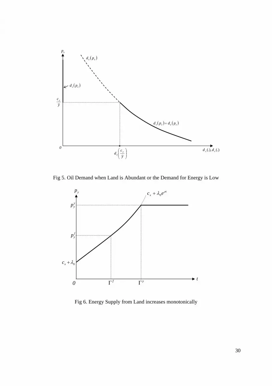
(c) Land is Abundant both for Food and Energy, 0yf == ππ :

Finally suppose land is abundant or the demand for food and energy is small. Then

ycpp yyy

fy == . For any price of energyep that is higher than the trigger price ycy , all energy

has to be supplied by land and the demand for oil decreases from )( ycd ye to a value that is

indeterminate within the interval [ ])(,0 ycd ye . This is the case in which the land fuel acts as a

pure backstop at the price ycy , as shown in Fig. 5.

[Figure 5 here]

4. The Land Fuel in a Hotelling Model

In this section we impose dynamics on the above Ricardian framework. First we consider the

Hotelling model without any environmental regulation. This is problem (P) without the

constraint 0≥− ZZ . The modified condition (3) now becomes ( ) xxcyxu γλ −+=+′ and

conditions (8), (9) and (11) no longer hold.

Since yy

fyyx ppycc ≤≤< , the interval[ )y

yx p,c is nondegenerate. For any ( )xyy0 cp,0 −∈λ let

( )0xp λ be the Hotelling price of oil which must equal the marginal extraction cost augmented by

the scarcity rent of the resource, i.e., t0x0x ec)(p ρλλ += . Let ( )0

y λΓ be the time at which this

13

price is equal to yyp , i.e., ]ln)cp[ln()( 0x

yy

10

y λρλΓ −−= − . Then we must have 0d

d

0

y >λΓ

,

0lim y

cp xyy0

=−↑ Γλ and +∞=↓y

00

lim Γλ . A higher initial Hotelling rent will shorten the date of

exhaustion of oil.

Let ( )0X λ be the cumulative consumption of oil over the time interval )](,0[ 0y λΓ along this

Hotelling price path. The aggregate supply of oil is ( ) ( )∫= 0y

0

0xx0 dt))(p(dXλΓ λλ . We have 0

d

dX

0

<λ ,

0Xlimx

yy0 cp

=−↑λ and +∞=↓ Xlim00λ which suggests that the equation ( ) 0

0 XX =λ has a unique

solution given by the optimal value of the Hotelling rent of oil, absent environmental regulation.

As a function of 0X , the equilibrium rent is decreasing with 0lim 0X0

=∞↑ λ and xyy0

0Xcplim

0−=↓ λ .

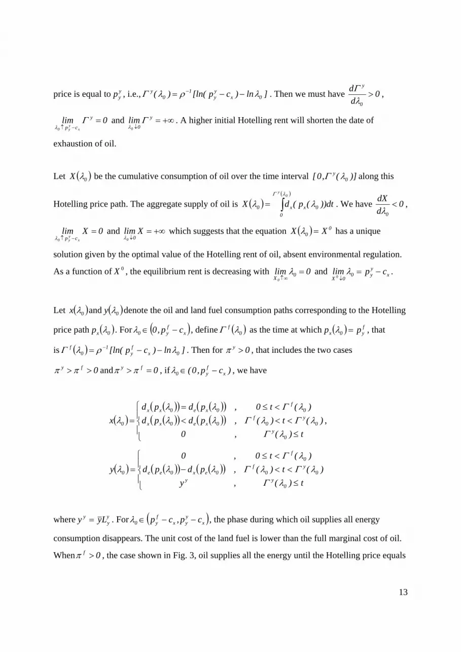
Let ( )0x λ and ( )0y λ denote the oil and land fuel consumption paths corresponding to the Hotelling

price path ( )0xp λ . For ( )xfy0 cp,0 −∈λ , define ( )0

f λΓ as the time at which ( ) fy0x pp =λ , that

is ( ) ]ln)cp[ln( 0xfy

10

f λρλΓ −−= − . Then for 0y >π , that includes the two cases

0fy >> ππ and 0fy => ππ , if )cp,0( xfy0 −∈λ , we have

( ) ( )( ) ( )( )( )( ) ( )( )⎪⎩⎪⎨⎧

≤<<<

<≤==

t)(,0

)(t)(,pdpd

)(t0,pdpd

x

0y

0y

0f

0xe0xx

0f

0xe0xx

0 λΓλΓλΓλλ

λΓλλλ ,

( ) ( )( ) ( )( )⎪⎩⎪⎨⎧

≤<<−

<≤=

t)(,y

)(t)(,pdpd

)(t0,0

y

0yy

0y

0f

0ex0ee

0f

0 λΓλΓλΓλλ

λΓλ

where yy

y Lyy = . For ( )xyyx

fy0 cp,cp −−∈λ , the phase during which oil supplies all energy

consumption disappears. The unit cost of the land fuel is lower than the full marginal cost of oil.

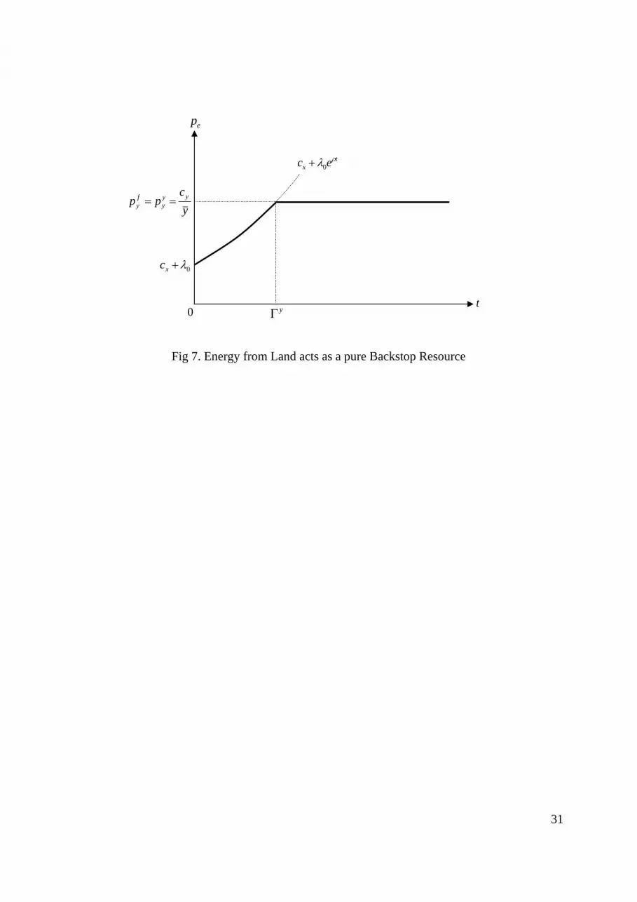
When 0f >π , the case shown in Fig. 3, oil supplies all the energy until the Hotelling price equals

14

the trigger price fyp . Above this price, the supply of oil is augmented by fuel from land. The

supply of the land fuel increases until oil is completely exhausted at priceyyp , as shown in Fig. 6.

When 0f =π but 0y >π , the supply of the land fuel is as shown in Fig.4. Oil supply is positive

in the entire price range( )yy

fy pp , . Oil is exhausted when the price reachesy

yp . Finally, when

0y =π , then ycpp yfy

yy == , the land fuel acts as a pure backstop resource. Only oil is supplied

until time yf ΓΓ = , shown in Fig. 7. The intermediate phase of simultaneous extraction that

occurred previously disappears.

[Figures 6 and 7 here]

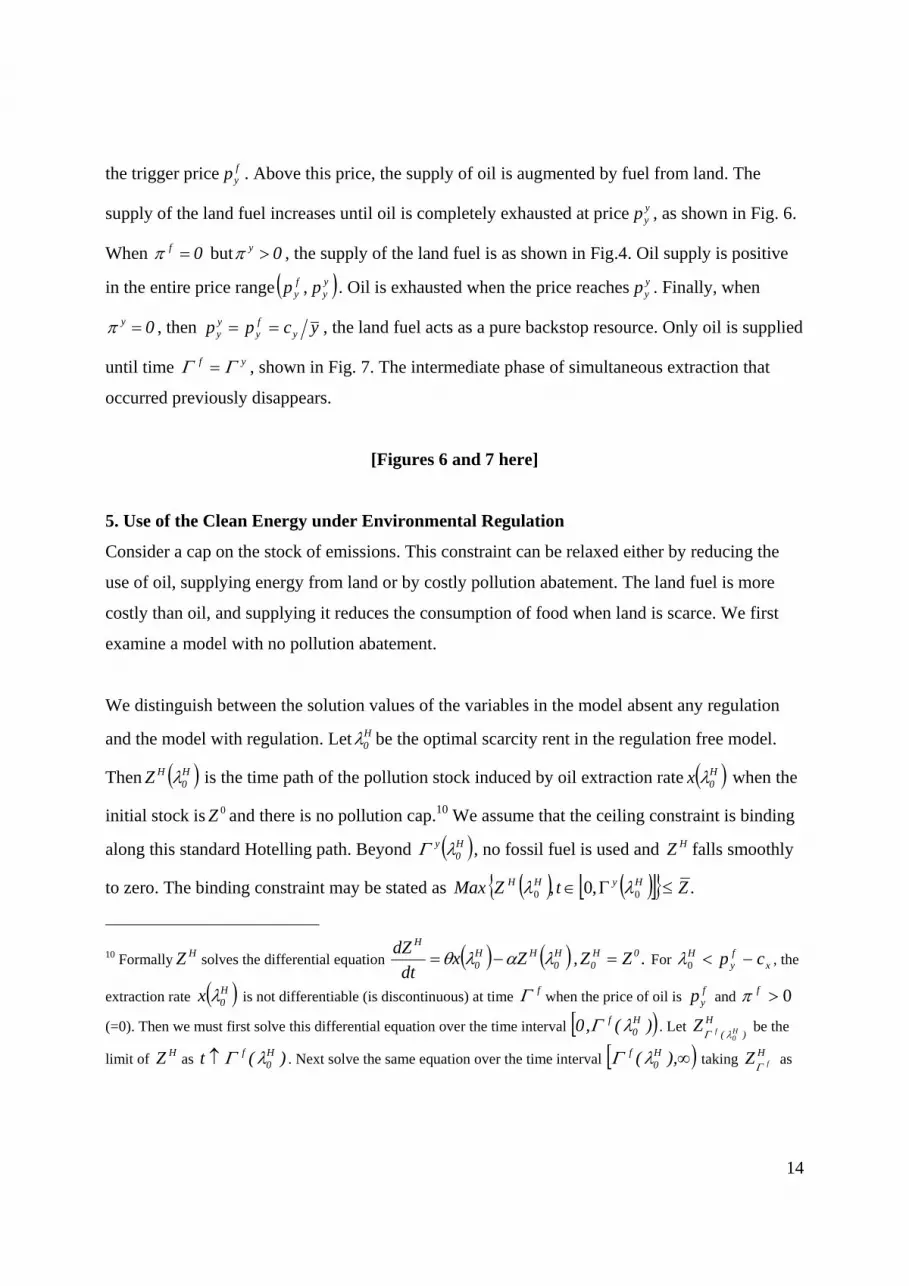
5. Use of the Clean Energy under Environmental Regulation

Consider a cap on the stock of emissions. This constraint can be relaxed either by reducing the

use of oil, supplying energy from land or by costly pollution abatement. The land fuel is more

costly than oil, and supplying it reduces the consumption of food when land is scarce. We first

examine a model with no pollution abatement.

We distinguish between the solution values of the variables in the model absent any regulation

and the model with regulation. LetH0λ be the optimal scarcity rent in the regulation free model.

Then ( )H0

HZ λ is the time path of the pollution stock induced by oil extraction rate( )H0x λ when the

initial stock is 0Z and there is no pollution cap.10 We assume that the ceiling constraint is binding

along this standard Hotelling path. Beyond ( )H0

y λΓ , no fossil fuel is used and HZ falls smoothly

to zero. The binding constraint may be stated as ( ) ( )[ ]{ } .,0, 00 ZtZMax HyHH ≤Γ∈ λλ

10 Formally HZ solves the differential equation ( ) ( ) .ZZ , Z xdt

dZ 0H0

H0

HH0

H =−= λαλθ For xfy

H cp −<0λ , the

extraction rate ( )H0x λ is not differentiable (is discontinuous) at time fΓ when the price of oil is f

yp and 0>fπ

(=0). Then we must first solve this differential equation over the time interval [ ))(,0 H0

f λΓ . Let H

)( H0

fZ λΓ be the

limit of HZ as )(t H0

f λΓ↑ . Next solve the same equation over the time interval [ )∞),( H0

f λΓ taking HfZΓ as

15

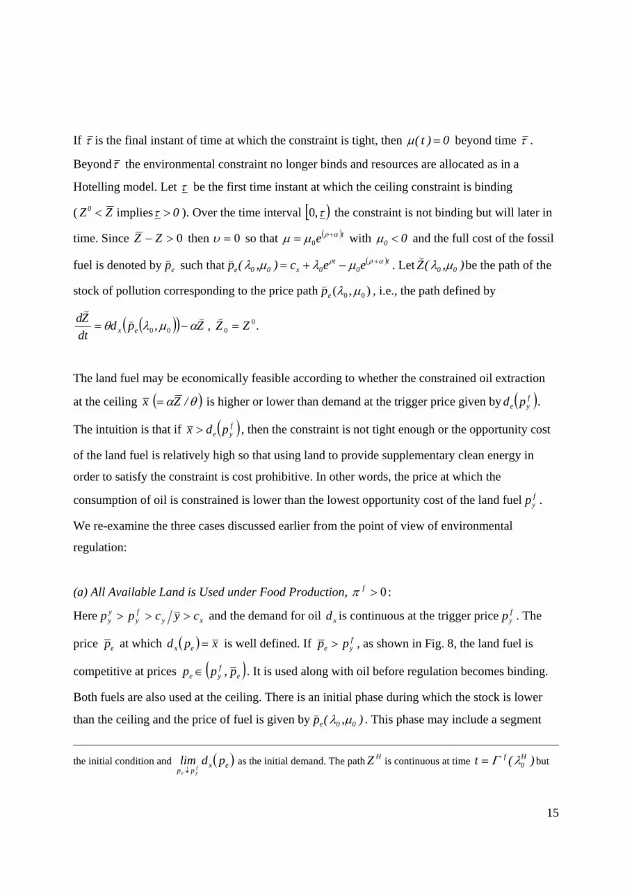
If τ is the final instant of time at which the constraint is tight, then 0)t( =µ beyond time τ .

Beyondτ the environmental constraint no longer binds and resources are allocated as in a

Hotelling model. Let τ be the first time instant at which the ceiling constraint is binding

( ZZ0 < implies 0>τ ). Over the time interval [ )τ,0 the constraint is not binding but will later in

time. Since 0>− ZZ then 0=υ so that ( )te αρµµ += 0 with 00 <µ and the full cost of the fossil

fuel is denoted byep(

such that ( )t0

t0x00e eec),(p αρρ µλµλ +−+=(

. Let ),(Z 00 µλ(be the path of the

stock of pollution corresponding to the price path ),( 00 µλep(

, i.e., the path defined by

( )( ) . , , 0000 ZZZpd

dt

Zdex =−= (((

(

αµλθ

The land fuel may be economically feasible according to whether the constrained oil extraction

at the ceiling x ( )θα /Z= is higher or lower than demand at the trigger price given by( )fye pd .

The intuition is that if ( )fye pdx > , then the constraint is not tight enough or the opportunity cost

of the land fuel is relatively high so that using land to provide supplementary clean energy in

order to satisfy the constraint is cost prohibitive. In other words, the price at which the

consumption of oil is constrained is lower than the lowest opportunity cost of the land fuel fyp .

We re-examine the three cases discussed earlier from the point of view of environmental

regulation:

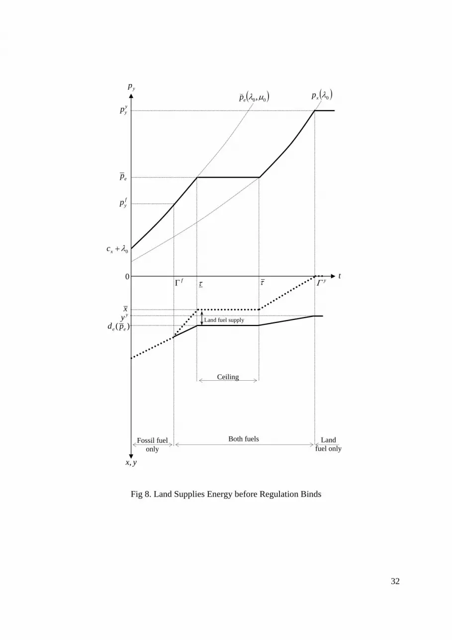
(a) All Available Land is Used under Food Production, 0>fπ :

Here xyfy

yy cycpp >>> and the demand for oil xd is continuous at the trigger pricefyp . The

price ep at which ( ) xpd ex = is well defined. If fye pp > , as shown in Fig. 8, the land fuel is

competitive at prices ( )efye ppp ,∈ . It is used along with oil before regulation becomes binding.

Both fuels are also used at the ceiling. There is an initial phase during which the stock is lower

than the ceiling and the price of fuel is given by ),(p 00e µλ(. This phase may include a segment

the initial condition and ( )ex

pppdlim

fye↓

as the initial demand. The pathHZ is continuous at time )(t H0

f λΓ= but

16

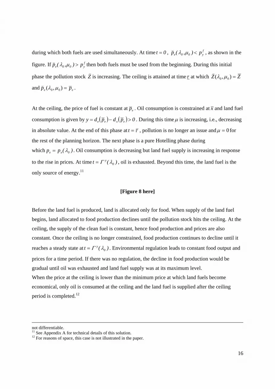
during which both fuels are used simultaneously. At time0t = , fy00e p),(p <µλ(

, as shown in the

figure. If fy00e p),(p >µλ(

then both fuels must be used from the beginning. During this initial

phase the pollution stock Z(

is increasing. The ceiling is attained at timeτ at which ZZ =),( 00 µλ(

and ee pp =),( 00 µλ(.

At the ceiling, the price of fuel is constant atep . Oil consumption is constrained atx and land fuel

consumption is given by ( ) ( ) 0pdpdy exee >−= . During this timeµ is increasing, i.e., decreasing

in absolute value. At the end of this phase atτ=t , pollution is no longer an issue and 0=µ for

the rest of the planning horizon. The next phase is a pure Hotelling phase during

which )(pp 0xe λ= . Oil consumption is decreasing but land fuel supply is increasing in response

to the rise in prices. At time )(t 0y λΓ= , oil is exhausted. Beyond this time, the land fuel is the

only source of energy.11

[Figure 8 here]

Before the land fuel is produced, land is allocated only for food. When supply of the land fuel

begins, land allocated to food production declines until the pollution stock hits the ceiling. At the

ceiling, the supply of the clean fuel is constant, hence food production and prices are also

constant. Once the ceiling is no longer constrained, food production continues to decline until it

reaches a steady state at )(t 0y λΓ= . Environmental regulation leads to constant food output and

prices for a time period. If there was no regulation, the decline in food production would be

gradual until oil was exhausted and land fuel supply was at its maximum level.

When the price at the ceiling is lower than the minimum price at which land fuels become

economical, only oil is consumed at the ceiling and the land fuel is supplied after the ceiling

period is completed.12

not differentiable. 11 See Appendix A for technical details of this solution. 12 For reasons of space, this case is not illustrated in the paper.

17

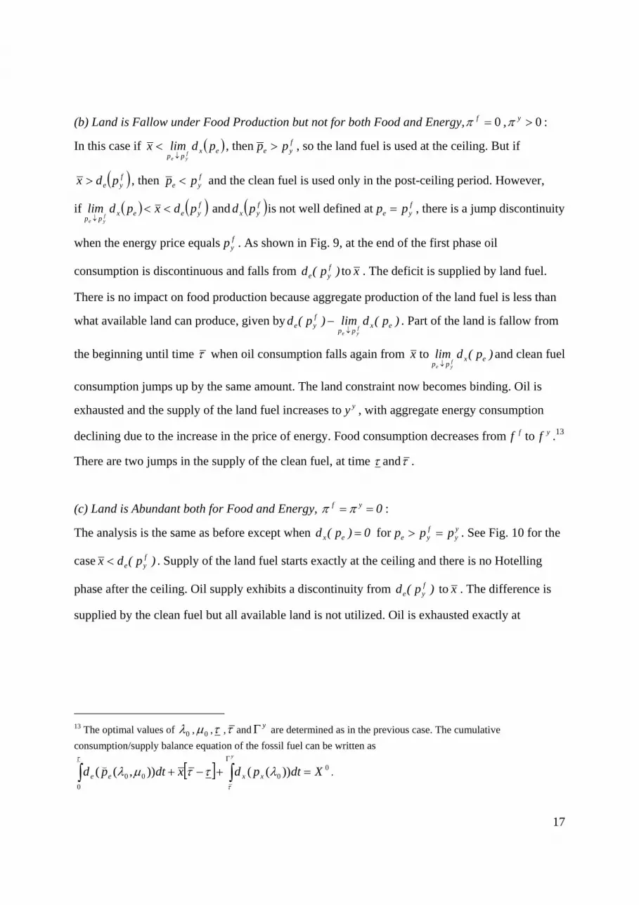
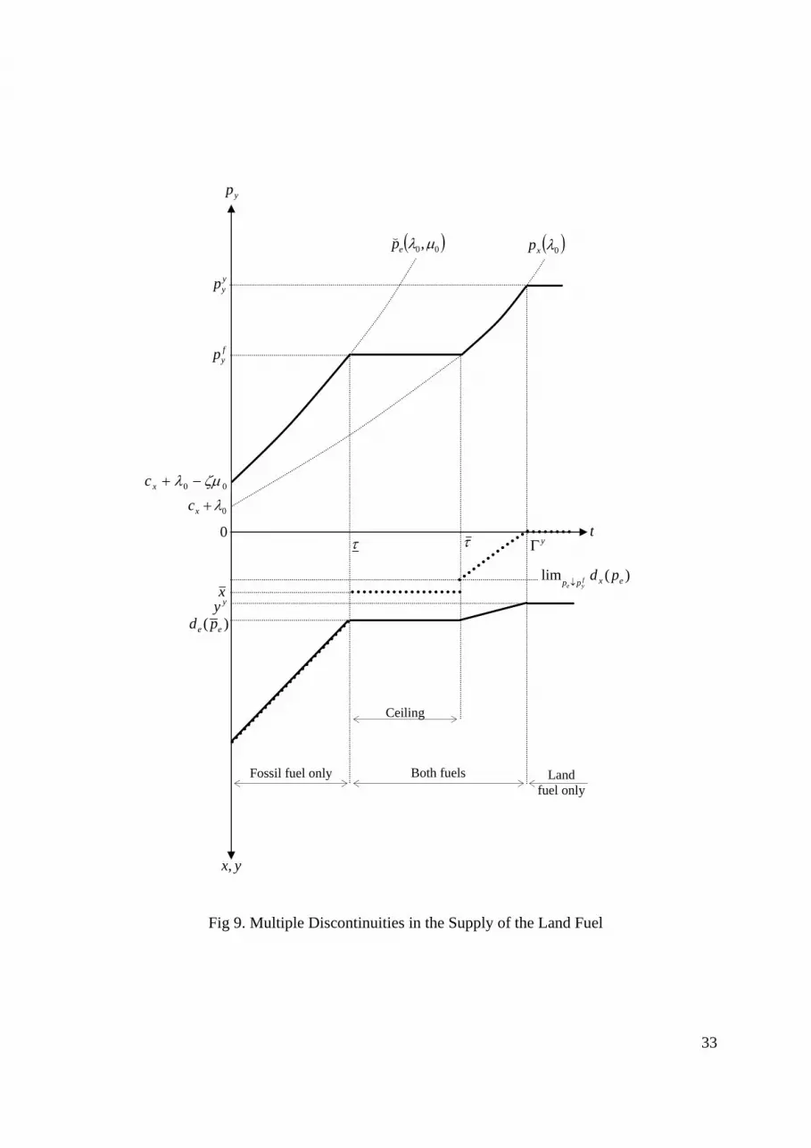
(b) Land is Fallow under Food Production but not for both Food and Energy,0=fπ , 0>yπ :

In this case if ( )expp

pdlimxfye↓

< , then fye pp > , so the land fuel is used at the ceiling. But if

( )fye pdx > , then f

ye pp < and the clean fuel is used only in the post-ceiling period. However,

if ( ) ( )fyeex

pppdxpdlim

fye

<<↓ and ( )fyx pd is not well defined at f

ye pp = , there is a jump discontinuity

when the energy price equalsfyp . As shown in Fig. 9, at the end of the first phase oil

consumption is discontinuous and falls from )p(d fye to x . The deficit is supplied by land fuel.

There is no impact on food production because aggregate production of the land fuel is less than

what available land can produce, given by )p(dlim)p(d expp

fye f

ye↓− . Part of the land is fallow from

the beginning until time τ when oil consumption falls again from x to )p(dlim expp f

ye↓and clean fuel

consumption jumps up by the same amount. The land constraint now becomes binding. Oil is

exhausted and the supply of the land fuel increases toyy , with aggregate energy consumption

declining due to the increase in the price of energy. Food consumption decreases fromff to yf .13

There are two jumps in the supply of the clean fuel, at time τ andτ .

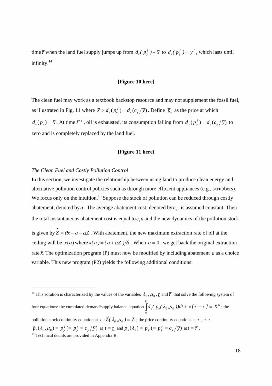
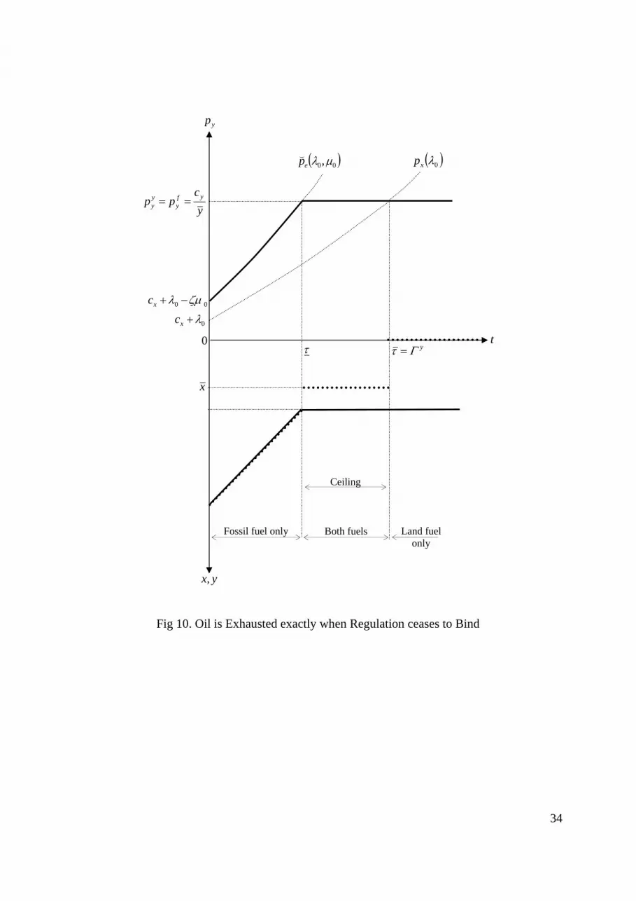
(c) Land is Abundant both for Food and Energy, 0yf == ππ :

The analysis is the same as before except when 0)p(d ex = for yy

fye ppp => . See Fig. 10 for the

case )p(dx fye< . Supply of the land fuel starts exactly at the ceiling and there is no Hotelling

phase after the ceiling. Oil supply exhibits a discontinuity from )p(d fye tox . The difference is

supplied by the clean fuel but all available land is not utilized. Oil is exhausted exactly at

13 The optimal values of 0λ , 0µ ,τ ,τ and yΓ are determined as in the previous case. The cumulative

consumption/supply balance equation of the fossil fuel can be written as

[ ] 00

0

00 ))(()),(( Xdtpdxdtpd

y

xxee =+−+ ∫∫ Γ

τ

τ λττµλ(.

18

timeτ when the land fuel supply jumps up from x)p(d fye − to ff

ye y)p(d = , which lasts until

infinity.14

[Figure 10 here]

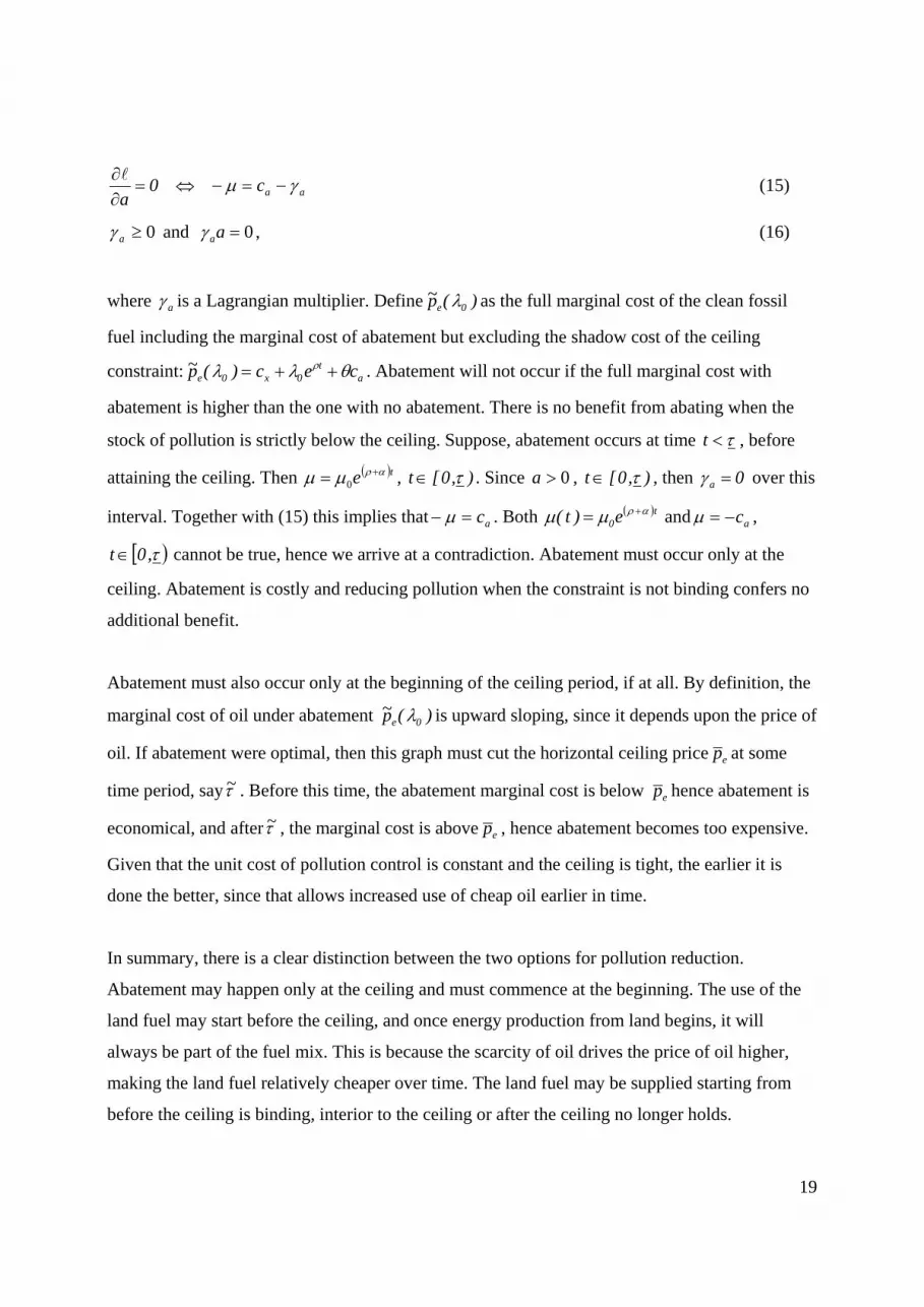
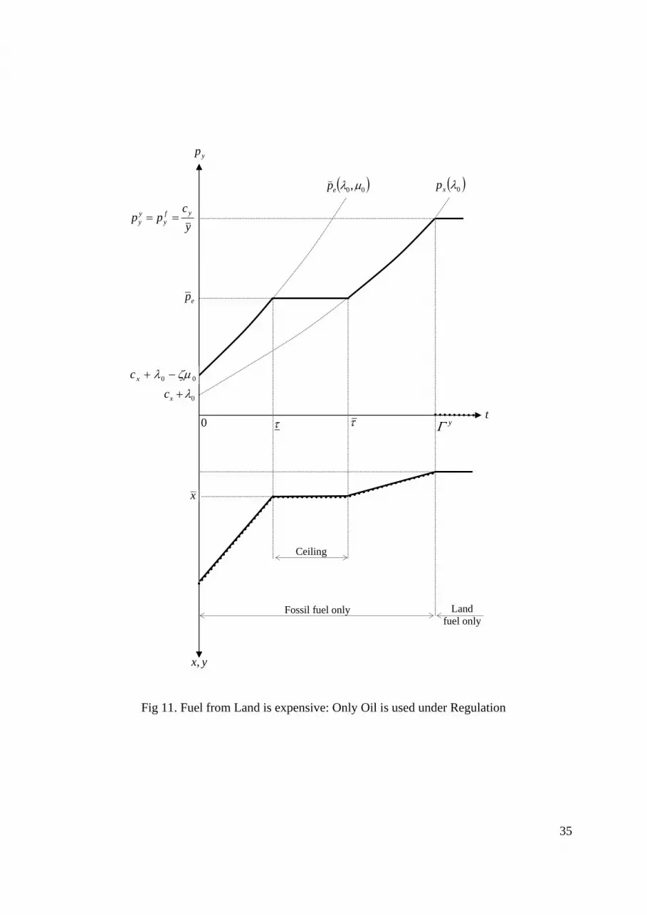
The clean fuel may work as a textbook backstop resource and may not supplement the fossil fuel,

as illustrated in Fig. 11 where )()( ycdpdx yef

ee => . Define ep as the price at which

xpd ee =)( . At time yΓ , oil is exhausted, its consumption falling from )()( ycdpd yefyx = to

zero and is completely replaced by the land fuel.

[Figure 11 here]

The Clean Fuel and Costly Pollution Control

In this section, we investigate the relationship between using land to produce clean energy and

alternative pollution control policies such as through more efficient appliances (e.g., scrubbers).

We focus only on the intuition.15 Suppose the stock of pollution can be reduced through costly

abatement, denoted bya . The average abatement cost, denoted byac , is assumed constant. Then

the total instantaneous abatement cost is equal toaca and the new dynamics of the pollution stock

is given by ZaxZ αθ −−=•. With abatement, the new maximum extraction rate of oil at the

ceiling will be )(ax where θα )Za()a(x += . When 0=a , we get back the original extraction

rate .x The optimization program (P) must now be modified by including abatement aas a choice

variable. This new program (P2) yields the following additional conditions:

14 This solution is characterized by the values of the variables 0λ , 0µ ,τ andτ that solve the following system of

four equations: the cumulated demand/supply balance equation 0

0

00ee X][xdt)),(p(d =−+∫ ττµλτ(

; the

pollution stock continuity equation at τ : Z),(Z 00 =µλ(; the price continuity equations at τ , τ :

)(),( 00 ycppp yyy

fye ===µλ(

at τ=t and )()( 0 ycppp yyy

fyx ===λ at τ=t .

15 Technical details are provided in Appendix B.

19

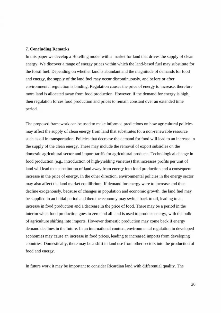
aac 0a

γµ −=−⇔=∂∂l

(15)

0≥aγ and 0 =aaγ , (16)

where aγ is a Lagrangian multiplier. Define )(p~ 0e λ as the full marginal cost of the clean fossil

fuel including the marginal cost of abatement but excluding the shadow cost of the ceiling

constraint: at

0x0e cec)(p~ θλλ ρ ++= . Abatement will not occur if the full marginal cost with

abatement is higher than the one with no abatement. There is no benefit from abating when the

stock of pollution is strictly below the ceiling. Suppose, abatement occurs at time τ<t , before

attaining the ceiling. Then ( )te αρµµ += 0 , ),0[t τ∈ . Since 0>a , ),0[t τ∈ , then 0a =γ over this

interval. Together with (15) this implies that ac=− µ . Both ( )t0e)t( αρµµ += and ac−=µ ,

[ )τ,0t∈ cannot be true, hence we arrive at a contradiction. Abatement must occur only at the

ceiling. Abatement is costly and reducing pollution when the constraint is not binding confers no

additional benefit.

Abatement must also occur only at the beginning of the ceiling period, if at all. By definition, the

marginal cost of oil under abatement )(p~ 0e λ is upward sloping, since it depends upon the price of

oil. If abatement were optimal, then this graph must cut the horizontal ceiling priceep at some

time period, sayτ~ . Before this time, the abatement marginal cost is below ep hence abatement is

economical, and afterτ~ , the marginal cost is aboveep , hence abatement becomes too expensive.

Given that the unit cost of pollution control is constant and the ceiling is tight, the earlier it is

done the better, since that allows increased use of cheap oil earlier in time.

In summary, there is a clear distinction between the two options for pollution reduction.

Abatement may happen only at the ceiling and must commence at the beginning. The use of the

land fuel may start before the ceiling, and once energy production from land begins, it will

always be part of the fuel mix. This is because the scarcity of oil drives the price of oil higher,

making the land fuel relatively cheaper over time. The land fuel may be supplied starting from

before the ceiling is binding, interior to the ceiling or after the ceiling no longer holds.

20

7. Concluding Remarks

In this paper we develop a Hotelling model with a market for land that drives the supply of clean

energy. We discover a range of energy prices within which the land-based fuel may substitute for

the fossil fuel. Depending on whether land is abundant and the magnitude of demands for food

and energy, the supply of the land fuel may occur discontinuously, and before or after

environmental regulation is binding. Regulation causes the price of energy to increase, therefore

more land is allocated away from food production. However, if the demand for energy is high,

then regulation forces food production and prices to remain constant over an extended time

period.

The proposed framework can be used to make informed predictions on how agricultural policies

may affect the supply of clean energy from land that substitutes for a non-renewable resource

such as oil in transportation. Policies that decrease the demand for food will lead to an increase in

the supply of the clean energy. These may include the removal of export subsidies on the

domestic agricultural sector and import tariffs for agricultural products. Technological change in

food production (e.g., introduction of high-yielding varieties) that increases profits per unit of

land will lead to a substitution of land away from energy into food production and a consequent

increase in the price of energy. In the other direction, environmental policies in the energy sector

may also affect the land market equilibrium. If demand for energy were to increase and then

decline exogenously, because of changes in population and economic growth, the land fuel may

be supplied in an initial period and then the economy may switch back to oil, leading to an

increase in food production and a decrease in the price of food. There may be a period in the

interim when food production goes to zero and all land is used to produce energy, with the bulk

of agriculture shifting into imports. However domestic production may come back if energy

demand declines in the future. In an international context, environmental regulation in developed

economies may cause an increase in food prices, leading to increased imports from developing

countries. Domestically, there may be a shift in land use from other sectors into the production of

food and energy.

In future work it may be important to consider Ricardian land with differential quality. The

21

scarcity of land may drive up food and energy prices, which in turn may determine equilibrium

land qualities in each sector as well as technological progress in these sectors, assumed constant

in this model. In a global economy, differential land qualities and demands may dictate the

optimal allocation of food production as well as land-based pollution control activities such as

sequestration through forestry.

22

References Chakravorty, U., B. Magne and M. Moreaux (2006), “A Hotelling Model with a Ceiling on the Stock of Pollution,” forthcoming, Journal of Economic Dynamics and Control. Farzin, Y.H. (1996), “Optimal Pricing of Environmental and Natural Resource Use with Stock Externalities,” Journal of Public Economics (62), 31-57. Forster, B.A., (1980), Optimal Energy Use in a Polluted Environment, Journal of Environmental Economics and Management (7), 321-33. Hoel, M., (1984), “Extraction of a Resource with a Substitute for Some of its Uses,” Canadian Journal of Economics (17), 593-602. Hoel, M., and S. Kverndokk (1996), Depletion of Fossil Fuels and the Impacts of Global Warming,” Resource and Energy Economics (18), 115-36. Hotelling, H., (1931), “The Economics of Exhaustible Resources,” Journal of Political Economy 39(2), 137-75. Ricardo, D., (1917), Principles of Political Economy and Taxation, Prometheus Books. Sinclair, P., (1994), “On the Optimal Trend of Fossil Fuel Taxation,” Oxford Economic Papers (46), 857-68. Tahvonen, O., (1997), “Fossil Fuels, Stock Externalities and Backstop Technologies,” Canadian Journal of Economics (30), 855-74. The New York Times (2006), “Corn Farmers Smile as Ethanol Prices Rise, but Experts on Food Supplies Worry,” by Matthew L. Wald, January 16. Toman, M.A., and C. Withagen (2000), “Accumulative Pollution, Clean Technology and Policy Design,” Resource and Energy Economics, (22), 367-84. Ulph, A., and D. Ulph (1994), “The Optimal Time Path of a Carbon Tax,” Oxford Economic Papers (46), 857-68.

23

Appendix A

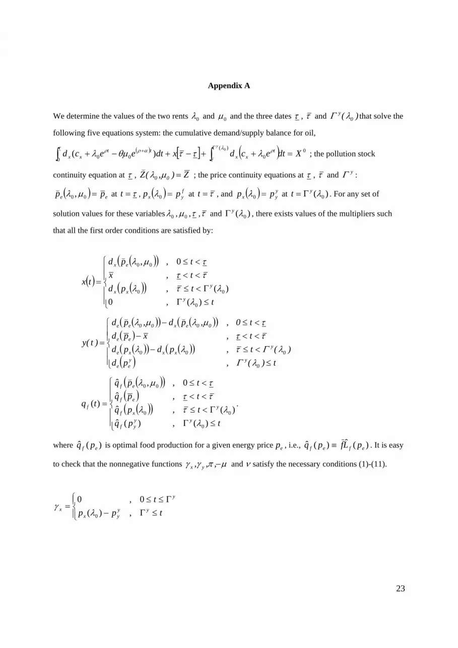
We determine the values of the two rents 0λ and 0µ and the three dates τ , τ and )( 0y λΓ that solve the

following five equations system: the cumulative demand/supply balance for oil,

( ) [ ] ( ) 0)(

00 00

0

)( Xdtecdxdteecdy

txx

ttxx =++−+−+ ∫∫ Γ+ λ

τραρτ ρ λττθµλ ; the pollution stock

continuity equation at τ , Z),(Z 00 =µλ( ; the price continuity equations at τ , τ and yΓ :

( ) ee pp =00,µλ( at τ=t , ( ) f

yx pp =0λ at τ=t , and ( ) yyx pp =0λ at )( 0λyt Γ= . For any set of

solution values for these variables0λ , 0µ ,τ ,τ and )( 0λyΓ , there exists values of the multipliers such

that all the first order conditions are satisfied by:

( )( )( )( )( )

⎪⎪⎩

⎪⎪⎨⎧

≤ΓΓ<≤

<<<≤

=t

tpd

tx

tpd

tx

y

yxx

ex

)(,0

)(,

,

0,,

0

00

00

λλτλ

τττµλ(

( )( ) ( )( )( )( )( ) ( )( )( )⎪⎪⎩⎪⎪⎨⎧

≤<≤−<<−<≤−

=t)(,pd

)(t,pdpd

t,xpd

t0,,pd,pd

)t(y

0yy

ee

0y

0xx0xe

ee

00ex00ee

λΓλΓτλλ

τττµλµλ ((

( )( )( )( )( )⎪⎪⎩

⎪⎪⎨⎧

≤ΓΓ<≤

<<<≤

=tpq

tpq

tpq

tpq

tq

yyyf

yxf

ef

ef

f

)(,)(ˆ

)(,ˆ

,ˆ

0,,ˆ

)(

0

00

00

λλτλ

τττµλ(

.

where )(ˆ ef pq is optimal food production for a given energy priceep , i.e., )(ˆ)(ˆ efef pLfpq ≡ . It is easy

to check that the nonnegative functions µπγγ −,,, yx and ν satisfy the necessary conditions (1)-(11).

⎪⎩⎪⎨⎧ ≤Γ−

Γ≤≤=tpp

tyy

yx

y

x ,)(

0,0

0λγ

24

⎪⎩⎪⎨⎧ ≤Γ

Γ≤≤−−=t

tcypf

ffye

y)(,0

)(0,),(

0

000 λλπµλγ (

⎪⎩⎪⎨⎧

≤ΓΓ≤≤Γ

Γ≤≤=

t

tp

t

yy

yfe

ff

)(,

)()(,)(ˆ

)(0,

0

00

0

λπλλπ

λππ

⎪⎩⎪⎨⎧

≤≤≤−−≤≤

=+

t

tpp

te

xe

t

τττθτµ

µαρ

,0

,/)(

0,)(0

, and

⎪⎩⎪⎨⎧

≤≤≤+−+−≤≤

= •

t

tppp

t

xxe τττθαρτ

υ,0

,/]))([(

0,0

.

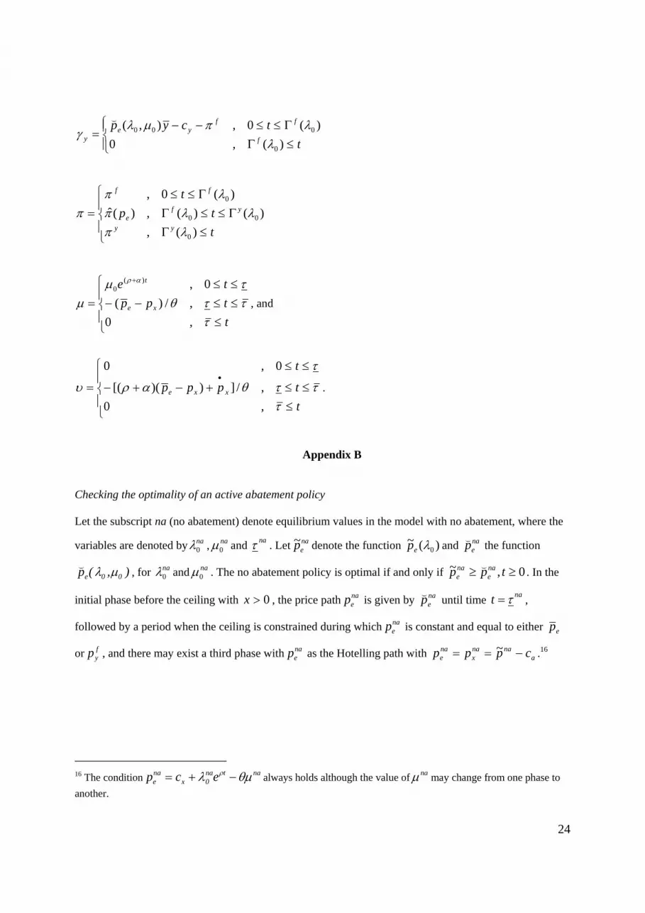
Appendix B

Checking the optimality of an active abatement policy Let the subscript na (no abatement) denote equilibrium values in the model with no abatement, where the

variables are denoted byna0λ , na

0µ and naτ . Let na

ep~ denote the function )(~0λep and na

ep(

the function

),(p 00e µλ(, for na

0λ and na0µ . The no abatement policy is optimal if and only if 0,~ ≥≥ tpp na

enae

(. In the

initial phase before the ceiling with 0>x , the price path naep is given by na

ep(

until time nat τ= ,

followed by a period when the ceiling is constrained during whichnaep is constant and equal to either ep

or fyp , and there may exist a third phase withna

ep as the Hotelling path with anana

xnae cppp −== ~ .16

16 The condition natna

0xnae ecp θµλ ρ −+= always holds although the value ofnaµ may change from one phase to

another.

25

Let nae

nae pp

(<~ over some time interval that includes τ , say ),( 21 ετετ +− nana, 2,1,0 => iiε . Assume

it is optimal not to abate and consider the interval during which nanae pp

(= . Since 0>x , then by (15),

and 0a ≥γ , we have µ−≥ac so that nae

nae pp

(≥~ , which is a contradiction. Thus it is optimal to abate.

However, consider the case when .0,~ ≥≥ tpp nae

nae

( At any time t such that 0>x , 0=aγ , na

enae pp~ >

which implies tac µ−> . By (15), aac γµ +−= and the preceding inequalities hold if and only if

0a >γ , i.e., if and only if 0=a . Thus it is optimal not to abate. The constrained solution with no

abatement is indeed the first best solution. In this case, the graph of naep~ shifts up and cuts the graph of

naep

( beyond time

naτ .

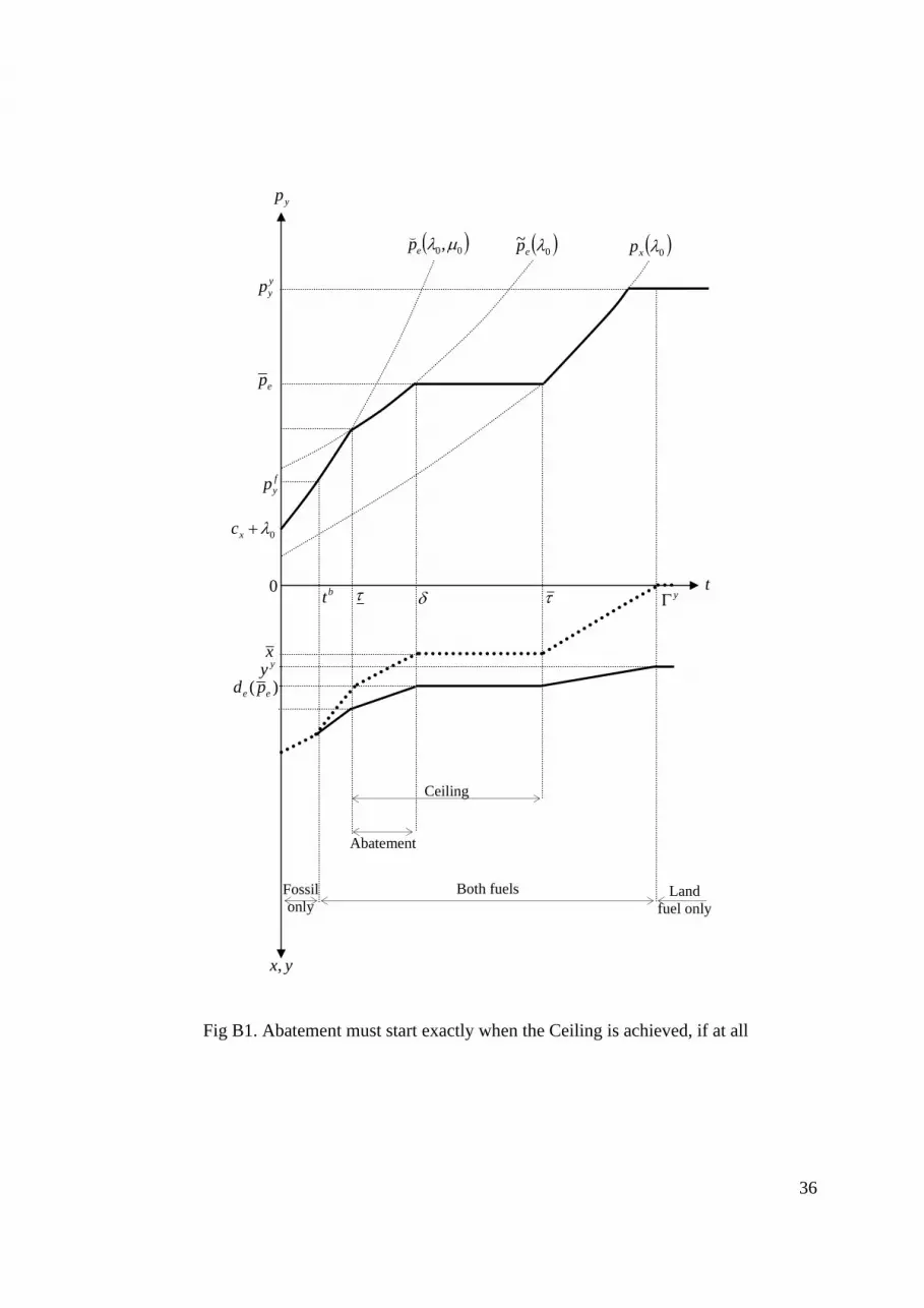
Determining the characteristics of the optimal path

Assume it is optimal to abate. We may have different scenarios according to the values of fyp , y

yp and

ep , one of which is illustrated in Fig B1. τ is the time at which the ceiling begins to be active and

abatement begins, δ the time at which the abatement must end andτ the time at which the ceiling

constraint ceases to be active.

[Figure B1 here]

We need to solve for0λ , 0µ , τ , δ , τ and yΓ from the following system of six equations: the

cumulative demand/supply balance equation for oil given by

( )( ) [ ] ( )( ) 000 00, Xdtpdxdtpd

y

xxex =+−+ ∫∫ Γτ

δ λδτµλ(; the pollution stock continuity equation at τ , the

time at which the ceiling is attained, ZZ =),( 00 µλ(; the price continuity equations - at time τ :

( ) ( )000~, λµλ ee pp =(

; time δ : ( ) ee pp =0~ λ ; time τ : ( ) ex pp =0λ and time yΓ : ( ) y

yx pp =0λ .

In Fig. B1 we assume that efy pp < and that f

yp is lower than ( )00,µλp(

at time τ . We denote by bt the

time at which ( ) fypp =00,µλ(

. Hence the ceiling constraint is first relaxed by both pollution abatement

26

and use of the land fuel followed only by the latter. But for a higher trigger pricefyp , still lower than ep ,

we could have three phases at the ceiling: first abatement, next abatement and use of land fuel and finally

use of the land fuel only. For efy pp > , the only option is to abate.

List of Symbols

U: utility function or gross surplus, ef uuU +≡

)( ii qu , { }efi ,∈ : gross surplus generated by good i

)q(u ii′ denoted by pi , { }efi ,∈

L : land endowment

{ }y,fi,Li ∈ : land allocated to good i, 0LLL yf ≥−−

y : quantity of land fuel

f , y : yields per unit of land, ff Lfq = , yLyy =

fc , yc : cost per unit of land

fc f / , ycy / : cost per unit output

X : stock of fossil fuel, 0X initial stock

)t(x : extraction rate of fossil fuel

xyqe +=

π : land rent

λ : scarcity rent of oil, 0λ : initial value, teρλλ 0=

Z : stock of pollutant

Z : pollution cap: 0)t(ZZ ≥−

θ : pollution per unit of fossil fuel

a : abatement

α : natural regeneration rate of pollution

0 given, )0( , 0 ≥−<=−=•ZZZZZZxZ αθ

θα )Za()a(x += : constrained oil consumption when ZZ = , )0(xx ≡

27

µ : shadow cost of the pollutant stock, 0µ initial value

ac : unit cost of abatement

t0x0x ec)(p ρλλ +=

at

0x0e cec)(p~ θλλ ρ ++=

( )t0

t0x00e eec),(p αρρ µλµλ +−+=(

If land is allocated only to food production, then

ffL : land allocated to food production

fπ : land rent ( ) y/cp fy

fy π+≡ : full marginal cost of land fuel for fππ =

If land is allocated to both food and fuel production, then

yfL , y

yL : land allocated to food and fuel, respectively

yπ : land rent ( ) ycp yy

yy /π+≡ : full marginal cost of land fuel for yππ =

fffff cLfufL −′≡ )()(π : land rent for land under food production

yyyyy cLyuyL −′≡ )()(π : land rent for land under fuel production, absent fossil fuel

( ) ]ln)cp[ln( 0xfy

10

f λρλΓ −−= − , defined for ( )xfy cp −∈ ,00λ

]ln)cp[ln()( 0xyy

10

y λρλΓ −−= − , defined for ( )xyy cp −∈ ,00λ

For a given price of energyep ,

)(ˆef pL , )(ˆ

ey pL : land allocation when rents are equal for food and fuel

)(ˆ epπ : land rent

)(ˆ)(ˆ eye pLypy = : output of land fuel

)(ˆ)(ˆ efef pLfpq = : output of food

)(ˆ)()( eeeex pypdpd −≡ : residual demand for oil

)( 0λx : oil consumption along path ( ) ( ) ( )( )000 λλλ xxx pdxp ≡=

)( 0λy : oil consumption along path ( ) ( ) ( )( )000ˆ: λλλ xfx pLyyp ≡

28

Fig 1. Land is used only for Food

Fig 2. Land is used both for Food and Clean Energy

0 Land

( )Lfπ

1fπ 2

fπ

LL ff =f

fL

rentLand

0

( )ff Lπfπ

yfL y

yL

( )yy Lπ

fL yL

yπ

L

0

yπ yπ

29

Fig 3. Energy Supply when Land is Scarce or Demand for Food is High

Fig 4. Energy Supply with Abundant Land or Low Demand for Food

0 (.)(.), ex dd( )fye pd( )y

ye pd

( )ee pd 1−

fyp

( )epy

( )ex pd 1−

( ) ( )eeex pdpd 11 −− =

yyp

yp

0 (.)(.), ex dd( )fye pd( )y

ye pd

( )ee pd 1−

y

cp yf

y =

( )epy

( )ex pd 1−

( ) ( )eeex pdpd 11 −− =

yyp

yp

30

Fig 5. Oil Demand when Land is Abundant or the Demand for Energy is Low

Fig 6. Energy Supply from Land increases monotonically

( )ex pd

( ) ( )eeex pdpd =

( )ee pd

0(.)(.), ex dd

⎟⎟⎠⎞⎜⎜⎝

⎛y

cd y

e

ep

y

cy

yΓ0 fΓ

0λ+xc

tx ec ρλ0+

yyp

fyp

yp

t

31

Fig 7. Energy from Land acts as a pure Backstop Resource

yΓ

0λ+xc

y

cpp yy

yfy ==

ep

t0

tx ec ρλ0+

32

Fig 8. Land Supplies Energy before Regulation Binds

Land fuel supply

Ceiling

Fossil fuel only

Both fuels Land fuel only

( )0λxp( )00,µλep(

yx,

0λ+xc

yyp

fyp

t

ep

yp

0 τ τxyy)( ee pd

yΓfΓ

33

Fig 9. Multiple Discontinuities in the Supply of the Land Fuel

Ceiling

Fossil fuel only Both fuels Land fuel only

( )00,µλep(

yx,

0λ+xc

yyp

fyp

tτ τ

00 ζµλ −+xc

yp

0yΓ

( )0λxp

xyy)( ee pd

)(lim expppdf

ye↓

34

Fig 10. Oil is Exhausted exactly when Regulation ceases to Bind

Ceiling

Fossil fuel only Both fuels Land fuel only

( )0λxp( )00,µλep(

yx,

0λ+xc

y

cpp yf

yyy ==

tτ yΓτ =x

00 ζµλ −+xc

yp

0

35

Fig 11. Fuel from Land is expensive: Only Oil is used under Regulation

Ceiling

Fossil fuel only Land fuel only

( )0λxp( )00,µλep(

yx,

0λ+xc

ep

tτ τ

x

00 ζµλ −+xc

yp

0

y

cpp yf

yyy ==

yΓ

36

Fig B1. Abatement must start exactly when the Ceiling is achieved, if at all

Ceiling

Fossil only

Both fuels Land fuel only

( )0λxp( )00,µλep(

yx,

0λ+xc

yyp

fyp

t

ep

yp

0 τ τxyy)( ee pd

( )0~ λep

yΓδbt

Abatement