3-D seismic stratigraphic inversion applied toan oilfield offshore of Angola

Francisco da Cunha, Sonogol Fernando Moraes, Uenf Paul Johann, Petrobras

Abstract

The integration of well log data, poststack 3-D seismic data and conceptual geological knowledge (structural and stratigraphic) provides accurate information for reservoir modeling and improve the implementation of efficient well developments planning.

Stratigraphic deconvolution aims at improving the resolution which is here of paramount importance (Brac et al, 1988). Seismic data gives indirect three-dimensional information about the reservoir properties that can be integrated with well log derived information.

For seismic inversion approach the key wells from the area of study, were sonic and neutron-density log, were edited and processed through careful petrophysical analysis. Geological markers near and at the reservoir levels for these wells were also interpreted to calibrate the regional seismic interpretation.

The stratigraphic seismic inversion consists of calibrating to tie key geological intervals from the wells with the seismic horizons to build a 3-D initial model, and finally going through the inversion procedure to match seismic amplitudes by updating the acoustic impedance model.

The initial model, an 3-D acoustic impedance model, is buiding from the interpolation of well log information. The inversion methodology is carried out in an time window. We use the trace amplitudes as the constraints. The initial acoustic impedance model is modified through an iterative procedure until the seismic synthetics volume generated from the updated model match the real seismic data. The end product of the inversion procedure is a 3-D inverted acoustic impedance and associated reflectivity volumes.

Introduction This methodology will be illustrated on an field discovered in a water depth of approximately 600m, within the Lower Congo Basin, offshore of Angola, encompassing a Tertiary clastics of the Malembo Formation setting. The field lies in elongate trending regional growth fault. The hydrocarbon bearing occur on the hanging wall flank of this growth faulting, The wells have tested Upper to Middle Miocene, encountering biodegraded oil and shows gas. The sand reservoir sequences consisting of relatively thin layers are very porous and permeable. The main reservoirs objectives are the deltaic sands of the Middle and Upper Miocene turbiditic. The seal is supported by major rollover growth faulting, by dip and an thick marine clay (Top Miocene regional overlying the RS3T horizon). The structure of the field in study complex model is fairly typical of marine passive margin successions, which tectonic and sedimentary evolution is closely linked to the Neocomian breakup of Gondwana and subsequent opening of the South Atlantic Ocean. The stratigraphic column is a classical rift/drift sequence. The field in study is located in one series of late Tertiary depot throughs within the Miocene thick, and is controlled by rollover into a westerly hading growth faulting, which defines the eastern limit of the field.

The complex depositional system represent fully marine environment, probably in a distal shelf to upper bathyal setting a base of slope comprising a series of sand having been deposited during turbiditic discharges from the shelf generating different reservoir sand levels in the depth This project is largely based on the 3-D seismic data, covering about 231 Km², with emphasis placed on the preservation of true amplitudes. Data quality shows some amplitude distorsion and poor quality where occur a conjuction of pull-down and absorption effects. Structural control from seismic interpretation is good along the field. For this instance, decided to pick the fault pattern after inversion the data. Vertical and lateral sand distribution vary widely in the eastern and northern flanks of the field. Seismic resolution is low due presence of extremely high amplitudes in the gas cap zone The wells used for calibration are posted on the map, the southern PG-1 well and the northern PG-2 deviated well with two side-track. Despite the sand/shale impedance contrast, the amplitude map obtained by extracting amplitudes along the determined layering, image clearly seismic facies separation between PG-1 and PG-2. The main sources of uncertainty come from the net/gross ratio, the variability of petrophysical properties and the OWC and GOC location.

The objective of the study presented here is to show a particular methodology for using integrated tools in cases where the amount of well information is sparse in order

- to identify the internal reservoir architecture of the field

- better to characterize fluid contacts locations - to evaluate the possible existence of

communication or not at reservoir levels between the wells PG-1 and PG-2

- to create numerical model to allow the comparison of alternative field development scenarios and revise the reserves estimate for to remove the risk associated at the field development.

Principles of the methodology In order to achieve the proposed objectives, the project was approached in four part effort. First, a partial data inventory was made for the area of study. The purpose of the inventory was to determine all subsurface data available including log, core, core analysis data, VSP, checkshot survey, for the wells and 3D seismic data. Secondly, well logs were formatted in software SAS, and then loaded in Easytrace for editing, processing and modeling 1D. Synthetic seismograms were generated for each well in order to correlate well to seismic. For the synthetic seismogram generation in Easytrace, the wirelines logs were transformed from depth to time domain, followed the extraction of an precise source wavelet at each well which, when convolved with the reflectivity series, generates synthetic trace. By average of the all wavelets generated, have produced a single best wavelet representative. Four seismic horizons were roughly conducted to provide the time window (top & base of the reservoir, more two internal control horizons), structural architecture of the field and to serve as initial model for the process of the inversion. Thirdly, by accounting for seismic amplitudes, seismic interpretation, petrophysical data and geologic knowledge we were able to generate inverted volume of acoustic impedance. And finally, the inverted volume were integrated, and the horizon and fault interpretation were refined based on the inversion results. Based on local petrophysical relationships and geostatistical approaches, porosity variations could be estimated from acoustic impedance layers, and porosity maps produced for each reservoir interval. A geologic modeling was generated as input for the location of the new well planning.

Conclusions Acoustic impedance interpretation provides better indication of reservoir distribution than conventional seismic data, even thin reservoir sands. The seismic stratigraphic inversion adds substantial information to the original seismic data and to refine the drilling planning of the new wells. The results demonstrate a clear potential for use of the integrated system, coupled with a wireline well, seismic, core. Major advantages of this methodology are that it is conclusive and it provides detailed image of trhe reservoir. Recommendations Further study should be cconducted to explore the full capabilities of this methodology it may be accepted for use by several utilities in reservoir modeling. Possible limitations include application for poor reservoir conditions. Acknowledgements The authors wish to thank the Sonangol, Petrobras and Uenf for permission to publish this work Bibliography Johann, P., 1997, “ Inversion sismostratigraphique et

simulations stochastiques en 3-D” . Ph.D Thesis, Paris VI (Pierre et Marie Curie).

Johann, P., 1999, “Seismic Geoinversion as a Horizontal Well Positioning Tool: Applications in the Marlim and Barracuda Fields, Deep-Water Campos Basin” .

Figure 1 – Angola offshore blocks localization map. Figure 2 – Amplitude section with structural and stratigraphic framework of Angola offshore

reservoir

Figure 3 – 3-D stratigraphic inversion methodology. Figura 4 – Acoustic impedance after stratigraphic inversion.

ABSTRACT

The extrapolation of sonic profiles in oil industry is a routine for the geophysicists. A good

correlation between geological data in wells and seismic reflectors in a seismic line is necessary to reach good results in oil prospection. If a VSP(Vertical Seismic Profile) is available nearby an exploratory or development well, this routine becomes easy. Commonly the only available information is the sonic log, which in general doesn’t starts at the surface. So, the geophysicist begins compiling and integrating technical data from different sources: seismic velocities, geological information, velocity surveys, regional velocity pattern, sonic profiles, etc. Even after a good job, the definition of a velocity to extrapolate sonic data to surface is not an easy task. One usual decision is to use the interval velocity at the beginning of the sonic profile as the interval velocity up to the surface.

In this paper is proposed a simple and effective method to extrapolate sonic profiles: basically it is an interactive computer based application where the user may decide which velocity is good to do this extrapolation. The application creates and integrates velocities starting from the surface that rise exponentially and reach the beginning of sonic profile, then starts integrating the sonic profile. Visually the user may decide: the velocity used to extrapolate is too high, too low or good enough. If this velocity is not good, a visual inspection makes clear that the velocity gradient of the extrapolation doesn’t fit the velocity gradient at the beginning of the integrated sonic profile.

INTRODUCTION

One way to compute TxD (time x depth) curves is to use the data from the sonic profile. The sonic

time integration and extrapolation gives a complete relation of time with depth, and it may be written as: S-1 F

T(Z) = Σ 1/Ve + Σ 1/Vs , (1)

Z=1 Z=S where T(Z) = time as a function of depth Ve = extrapolation velocity Vs = sonic velocity S = initial depth of sonic F = final depth of sonic

The key to solve equation (1) is to decide a good value to be used as Ve. Approximated values may

be obtained mainly after some interpretation of technical information found in velocity surveys, seismic data, geology and regional velocity pattern of sedimentary layers. Sometimes the definition of Ve is not easy and a bad definition may imply a complete failure of a petroleum industry project. Also, a project can be discarded as no economic when in reality it is economic. Recently, in our company we had an example of this type of situation. An old standby project became attractive due to changes in gas/oil demand and we

A simple and effective method to extrapolate sonic profiles to the surface

José Adauto de Souza

Petrobras SA

JOSÉ ADAUTO DE SOUZA

2

start a new evaluation. The planning was to drill a wildcat in a new structure nearby an oil/gas field, based on seismic lines. There are no seismic lines over the oil/gas field, due to geographical and environmental constraints. So, the conversion of depths of field wells to time is basic to estimate gas/oil and oil/water contacts in the planned wildcat. At the end we concluded that the project was not attractive due to changes in net-pay, total area and fluid percentage: the project became an oil project and not a gas project, as anticipated in the old evaluation. Mainly those changes were due to a new interpretation of sonic extrapolation velocity of wells from the oil/gas field.

THE METHOD

The velocity gradient of geological layers has an exponential decay with depth: velocities change

more rapidly at shallower depths. The use of a constant velocity (Ve) to extrapolate the sonic log disagrees with this property. This disagreement doesn’t imply in failures, if Ve is good enough and considering that the target zones as a general rule are below the beginning depth of the sonic profile. Why not to use this property (gradient with a exponential decay) to solve for Ve? The method presented here use this property and give us a nice chance to compute the extrapolation velocity. Basically, it builds a velocity curve starting from a user given value at the surface and an ending value at the beginning depth of sonic survey, rising exponentially. After this, the velocity sonic values are integrated to complete the TxD curve. The complete integration may be written as: S-1 F

T(Z) = Σ 1/Vi + Σ 1/Vs, (2)

Z=1 Z=S Vi(Z) = V0*EXP(cZ), (3) S-1

Vf(S) = { Σ Vi(Z) } / (S-1), (4) Z=1 where T(Z) = time as a function of depth Vi(Z) = interval velocity in the extrapolation zone (computed by application) Vf(S) = average extrapolation velocity at depth S-1(user defined) V0 = velocity at surface (user defined) c = constant value (computed by application) Z = actual depth Vs = sonic interval velocity S = initial depth of sonic F = final depth of sonic EXP = exponential with neper constant e

The constant c is computed by doing computer iterations. The definition of an initial value to be V0

is not important, only it must be lower than the average velocity Vf at the end of the extrapolation zone. It is common to use 1500 m/s for Tertiary basins and 2000 m/s for Lower Cretaceous basins as V0 value. Vf must be higher than V0 and this value is obtained after some interactive actions between the user and a Pc (personal computer) graphic application based on equations (2), (3) and (4). The user defines Vf visually, when the extrapolated velocity gradient is similar to the integrated velocity gradient at the beginning of the sonic profile. This will not work very well if the lithology in the extrapolated zone has a velocity gradient completely different compared with the velocity gradient present at the beginning of the zone covered by the sonic. One example of this occurs when the well has clastic sediments in the extrapolated zone and limestones immediately below. Figure 1 presents an output graphic image of an integrated and extrapolated sonic profile. The green curve was computed extrapolating a velocity function from V0 = 1800 m/s to Vf = 2000 m/s, till the magenta rectangle close to 200 ms and 200 m (x,y). The magenta rectangle gives the position where the sonic profile starts. Nearby this position there is a blue straight line that represents the velocity gradient at the beginning of the sonic profile. Clearly this blue line is moving away from the green line, which means that the velocity

A simple and effective method to extrapolate sonic profiles to surface

3

gradient defined by the velocity Vf at the end of the extrapolation is different if compared with the gradient of the sonic. Similarly, figure 2 shows that the blue line is parallel to the green line: the extrapolated gradient is close to the sonic gradient (Vf=2440 m/s). Figure 3 shows another curve with Vf=3000 m/s and is easy to interpret that the blue straight line is crossing the green curve: in this case the velocity gradient in the extrapolated zone is smaller than that of the sonic profile.

So, we may summarize: a) A Vf lower than the average velocity at the beginning of the sonic produces an image where the

blue curve moves away from the green curve(figure 1). Vf may be interpreted as lower than the good one.

b) A Vf higher than the average velocity at the beginning of the sonic produces an image where the blue curve crosses the green curve(figure 3). Vf may be interpreted as higher than the good one.

c) A Vf close to the average velocity at the beginning of the sonic produces an image where the blue curve is quite parallel to the green curve(figure 2). Vf may be interpreted as being a good velocity to extrapolate the sonic curve.

It is important to mention that the visual selection to define Vf is sensible to changes of 10 m/s,

meaning this definition is quite precise. Figure 4 presents a final interactive result (complete well) where the interpreter has defined an extrapolation average velocity Vf. In the right hand part of the figure a red curve represents the sonic readings and a colored column represents the lithologies. In the left two curves can be seen: the magenta (average velocities) and the red (interval velocities). In the same figure the green line (TxD extrapolated and integrated) has good fit with some blue boxes, that are data from a VSP survey. An additional output of the computer application is a columnar ASCII file including depths, two-way times, average velocities and interval velocities of the well.

Figure 1 – Extrapolation with Vf = 2000 m/s

Figure 2 – Extrapolation with Vf = 2440 m/s

JOSÉ ADAUTO DE SOUZA

4

CONCLUSIONS A simple and effective method to extrapolate sonic curves to surface has been presented. Basically, it solves the problem using the velocity gradient of the geological layers. An exponential decay curve is used to compute and integrate a complete set of interval velocities along the extrapolation zone, where the sonic has no readings. The method is sensitive to variations of 10 m/s in the computation of the extrapolation velocity, what means that it is very precise. A velocity mistake of 10 m/s in a extrapolated zone of 300 m using 2000 m/s as Vf introduces one error of 1.5 ms or 1.5 m. In the example showed in the figures, the average velocity in the first 15 m covered by the sonic is 2959 m/s (depths 224 to 238 m). If the interpreter decides to use this velocity as the one to extrapolate the sonic (Vf), an error of 27 ms will be introduced, assuming that the velocity 2440 m/s is the correct one. You may do some immediate guesses if the length of the extrapolation zone is higher ant the velocities are lower: the error introduced rises rapidly to values higher than 50 ms.

The interpreter must be careful when lithologies in the extrapolation zone are quite different compared with the lithologies in the beginning of the sonic survey: this may result in velocity gradients quite different and the method may not work very well. Anyway, in this case, the method still gives a chance to compute the extrapolation velocity by using additional geological and geophysical information. REFERENCES - Duarte, O. O.,1997, Dicionário Enciclopédico Inglês-Português de Geofísica e Geologia, Sociedade Brasileira de Geofísica, 304 p. ACKNOWLEDGMENTS I would like to thank Petrobras for permission to present and publish this work.

Figure 3 – extrapolation with Vf = 3000 m/s m/s Figure 4 – final graphic output

Aplicação da Coerência Sísmica à Detecção de Feições Estratigráficas e EstruturaisRaul Dias Damasceno, PETROBRAS S.A., Brasil; Adelson Santos de Oliveira, PETROBRAS S.A., Brasil,André Gerhard, Brasil; Amin Bassrei, IF-CPGG-UFBA

Abstract

Seismic coherence, defined as the phase relationshipmaintenance through a set of reflectors, can be usedas an auxiliary tool in order to map stratigraphic andstructural seismic features. In this paper, the results ofsome coherence methods based on semblance, eig-genstructure, and shaping filters are showed. Eachmethod was applied to real and synthetic data in orderto compare their results in presence of different pa-rameters. An image processing method, namedmathematical morphology, was applied on the ob-tained coherence images in order to improve the con-tinuity of the seismic coherence features. In the con-clusion the results are discussed as well as the limita-tions and recommendations for each method.

IntroduçãoO conceito de volume de coerência sísmica, introdu-zido por Bahorich e Farmer (1995), vem despertandocada vez mais interesse, sendo utilizado no mapea-mento de feições estratigráficas e estruturais.

No trabalho original de Bahorich e Farmer (1995) acoerência é obtida através da correlação cruzada entretraços vizinhos. Gersztenkorn e Marfurt (1996) apre-sentam, como evolução de Bahorich e Farmer (1995),métodos baseados em semblance e autoestrutura.Nestes, toma-se como base a matriz de covariânciados dados sobre a qual os respectivos algoritmos sãoaplicados.

Luo et al. (1996) apresentou um método no qual acoerência é estimada através da diferença entre traçosadjacentes. Mais recentemente, Oliveira (1999), apre-sentou um método onde a coerência é obtida atravésda diferença quadrática entre filtros conformadorescalculados entre traços sísmicos adjacentes. Nestetrabalho, apresentamos o resultado parcial de experi-mentos realizados envolvendo os métodos citados,onde foram avaliadas as respostas destes frente àvariação de diversos atributos, como deslocamentovertical, variação de freqüência e conteúdo de ruídoaleatório dos dados.

Análise e comparação dos métodosA coerência é uma medida matemática da similarida-de. Quando aplicada aos dados sísmicos fornece umindicador da continuidade entre dois ou mais traçospreviamente janelados. Idealmente, o grau da conti-

nuidade sísmica é um indicador direto da continuida-de geológica. Quando aplicada ao delineamento defeições estratigráficas e estruturais, a coerência temobtido melhores resultados em dados tridimensionaismigrados em tempo ou profundidade, embora possater aplicação em qualquer etapa do processamento.

A análise e comparação entre os métodos foram reali-zadas a partir da aplicação a dados sintéticos e reais,frente a diversos atributos, como variação de freqüên-cia, fase, amplitude, bem como em situações geológi-cas distintas, como diferentes ângulos de mergulho erejeito de falhas.

Dois tipos de traços foram utilizados na geração dosdados sintéticos, um pulso tipo Gabor e cossenóides.Esta escolha foi feita em razão dos métodos não se-rem lineares, portanto o que acontece com um pulsonão é a soma do que acontece com suas componentesde Fourier. Como o dado real não é nem um pulso,nem uma cossenóide, procurou-se ter uma visão glo-bal do comportamento dos métodos baseada em seusextremos. Como unidade de medida padrão utiliza-ram-se os períodos dominantes, permitindo assim aextensão dos resultados obtidos aos dados reais apartir do conhecimento das freqüências contidas nes-tes. Os testes numéricos, bem como resultados analí-ticos, mostraram que os resultados obtidos são depen-dentes de diversas variáveis como o tamanho da ja-nela em relação ao período, nível de ruído, fase entrea janela e os dados, variação de amplitude, desloca-mento vertical (rejeito) e do relacionamento entreestas.

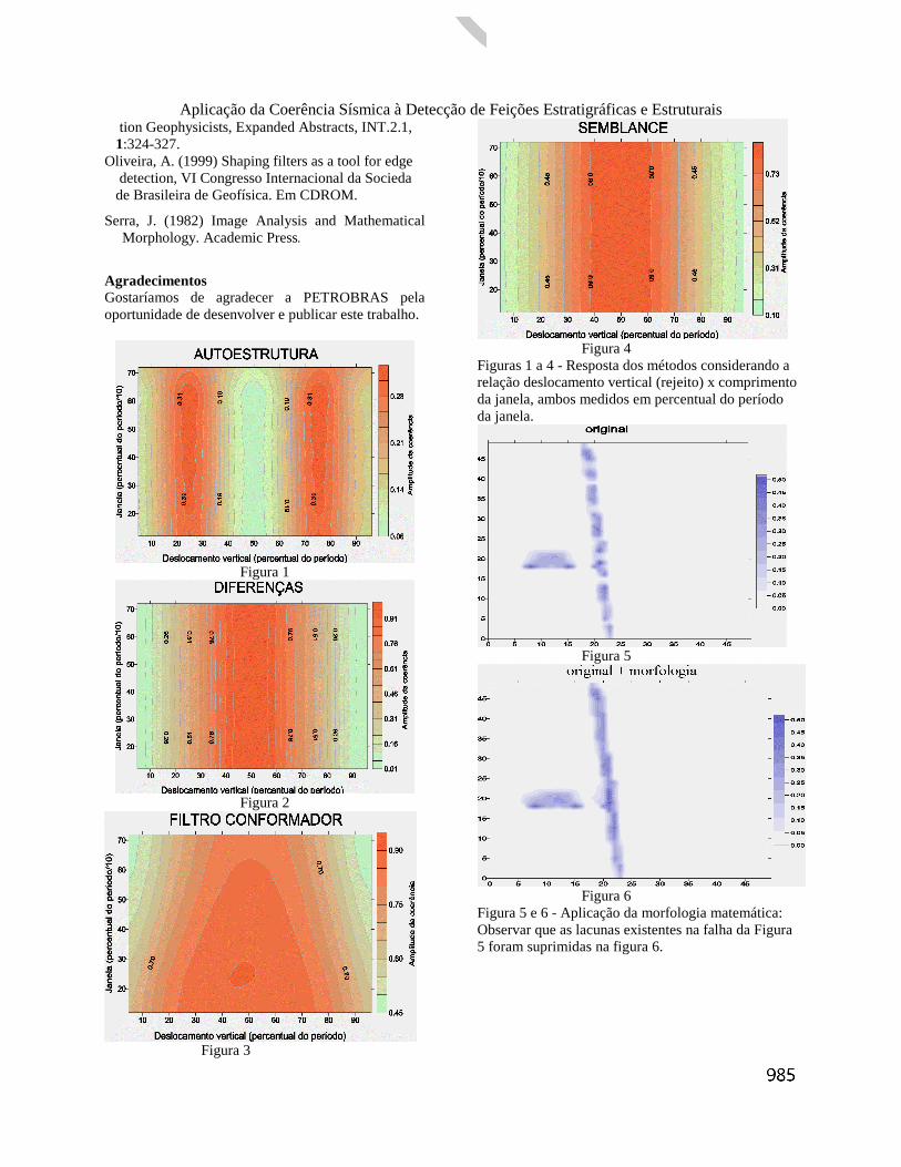
Deslocamentos verticais entre sinais de traços sísmi-cos vizinhos são descontinuidades comuns, sendoindicativas principalmente de falhamentos. Se imagi-narmos o deslocamento vertical como sendo dado poruma mudança de fase, outras estruturas podem serenglobadas nesta análise como canais, recifes, etc.Estas diferenças de fase entre traços vizinhos mostra-ram-se como o principal fator de sensibilização dosmétodos. Considerando a relação entre o desloca-mento vertical e o tamanho da janela, sendo ambas asgrandezas dadas em percentual do período, a pesquisamostrou que para os métodos de diferenças, filtroconformador e semblance a melhor resposta ocorrequando o deslocamento é máximo, ou seja, para umadiferença de fase de π. Já o método autoestruturaapresenta seu maior desempenho para deslocamentosde π/2, apresentando um mínimo em π (vide Figuras

Aplicação da Coerência Sísmica à Detecção de Feições Estratigráficas e Estruturais1 a 4). Este resultado é vantajoso em relação aosdemais métodos, visto que a faixa de melhor desem-penho é atingida mais rapidamente. A resolução ver-tical da resposta a ser obtida está diretamente relacio-nada ao tamanho da janela utilizada. O tamanho idealde janela é de um período dominante, embora so-mente o método autoestrutura tenha se mostradorestritivo a valores menores, de modo que a menorfreqüência dominante balizará o tamanho da janela aser utilizada.Os métodos são bastante sensíveis, sendo possívelmapearem-se pequenas descontinuidades da ordem dedécimos do período. Fatores limitantes ao desempe-nho são os níveis de ruído aleatório e o mergulho.

O nível de ruído mostrou -se o ponto de maior sensi-bilidade, principalmente em relação ao método dofiltro conformador. Nesta situação, o método de auto-estruturas apresenta o melhor desempenho, fato quepode explicar os ótimos resultados registrados pelaliteratura. Tal fato recomenda um tratamento acuradodos dados de modo a torná-los os mais livres possí-veis de ruídos principalmente no caso do conforma-dor. As Figuras 7 e 8 comparam a aplicação do méto-do do filtro conformador a dados com e sem umafiltragem FX respectivamente. A Figura 9 mostra amesma imagem obtida com o método semblancesobre dados com filtragem FX.

As limitações impostas pelo mergulho devem-se aofato da busca de coerência ocorrer no sentido hori-zontal de modo que as mudanças amostra a amostra,passam a ser vistas como descontinuidades. Para osmétodos de autoestrutura, diferenças e semblance énecessário uma busca do valor e direção de mergulhopreviamente à aplicação dos métodos. Esta buscaimplica em um maior esforço computacional, além daintrodução de imprecisões surgidas do processo deinterpolação. No caso do filtro conformador um in-cremento de mergulho constante traço a traço implicaem filtros formados por pulsos com deslocamentosiguais em relação ao lag zero, ou seja, já incorporan-do o efeito de mergulho. Os testes mostraram que apresença de mergulho exerce uma forte influênciasobre os métodos de diferenças e autoestruturas, e emmenor escala sobre o método semblance. O métododo filtro conformador, devido a sua metodologia, épraticamente imune ao mergulho.

Outros parâmetros que influenciam o desempenhodos métodos são a variação de amplitude e a fase dosdados em relação à janela. A fase em relação à janelaé um parâmetro que mostrou pouca importância po-dendo ser negligenciado. Já a variação de amplitudeinflui de forma direta no caso dos métodos autoes-

trutura, conformador e diferenças e inversa no casodo semblance.Tratamento das imagensO caráter policromático dos dados sísmicos faz comque a resposta dos métodos não seja uniforme emtoda a seção fazendo com que as estruturas mapeadasapresentem lacunas na imagem gerada. Visando obteruma imagem de melhor qualidade, através do preen-chimento de tais lacunas, aplicou-se um método cujoprincípio se baseia na teoria da morfologia matemáti-ca (Serra, 1975), cujo princípio é a descrição da ima-gem como regiões ou conjuntos. Os operadores sãoconstruídos pela combinação de operações elementa-res como união, intersecção e operações de composi-ção. Estes operadores e as operações da Morfologiamatemática são ferramentas para extração de infor-mações das imagens. As Figuras 5 e 6 ilustram aaplicação da morfologia matemática, mais especifi-camente do operador de fechamento.

ConclusõesEm razão dos resultados obtidos utilizando-se traçosgerados por um pulso Gabor e por cossenóides teremsido compatíveis, podemos estender o comportamentoobservado nos testes aos dados reais. Todos os méto-dos mostraram bons resultados e grande capacidadede detecção. Os métodos diferença vetorial e filtroconformador são mais sensíveis a pequenas variaçõessendo, portanto também mais susceptíveis ao ruídoaleatório. O método autoestrutura apresentou os me-lhores resultados, sendo mais eficiente em presençade ruídos. Em termos de procedimentos de rotina, osmétodos semblance e diferenças vetoriais são maisrápidos, podendo ser utilizados em uma abordagemmais expedita que exija menor precisão. Já o métodobaseado em filtros conformadores, embora apresentea vantagem de não depender dos mergulhos, nãoapresentou imagens tão nítidas quanto os demais, fatoque pode ser atribuído a utilização de um menor nú-mero de traços. A aplicação da morfologia matemáti-ca mostrou-se como uma ferramenta eficaz, permitin-do a recomposição de estruturas apenas parcialmentemapeadas pelos métodos de detecção.

ReferênciasBahorich, M. e Farmer, S. (1995) 3-d seismic discon tinuity for faults and stratigraphic features: The Coherence cube, The Leading Edge, 10:1053-1058Gesztenkorn, A. e Marfurt, K. J. (1996) 3-d seismic discontinuity for faults and stratigraphic, 66th Ann. Internat. Mtg., Society of Exploration Geophysi- cists, Expanded Abstracts, INT.2.2, 1:328-331.Luo, Y.; Higgs, W. e Kowalik, W. (1996) Edge detec tion and stratigraphic analysis using 3d seismic data, 66th Ann. Internat. Mtg., Society of Explora

Aplicação da Coerência Sísmica à Detecção de Feições Estratigráficas e Estruturais tion Geophysicists, Expanded Abstracts, INT.2.1, 1:324-327.Oliveira, A. (1999) Shaping filters as a tool for edge detection, VI Congresso Internacional da Socieda de Brasileira de Geofísica. Em CDROM.

Serra, J. (1982) Image Analysis and MathematicalMorphology. Academic Press.

AgradecimentosGostaríamos de agradecer a PETROBRAS pelaoportunidade de desenvolver e publicar este trabalho.

Figura 1

Figura 2

Figura 3

Figura 4Figuras 1 a 4 - Resposta dos métodos considerando arelação deslocamento vertical (rejeito) x comprimentoda janela, ambos medidos em percentual do períododa janela.

Figura 5

Figura 6Figura 5 e 6 - Aplicação da morfologia matemática:Observar que as lacunas existentes na falha da Figura5 foram suprimidas na figura 6.

Figura 7 - Aplicação do método do filtro conformador.

Figura 8 - Idem da Figura 7, mas sobre dados onde foi aplicada previamente uma filtragem FX.

Figura 9 - Aplicação do método Semblance sobre os dados utilizados na Figura 8.

Borehole Seismic for imaging below surface basalt in Volcán Auca Mahuida Field, Neuquénbasin, Argentina.

Luis Pianelli, Repsol-YPF, ArgentinaEmilio Sanchez Repsol-YPF, ArgentinaAndres Vottero Repsol-YPF, ArgentinaEduardo Corti, Schlumberger, ArgentinaFlavia Croce, Schlumberger, Argentina

AbstractSurface seismic response in volcanic areas covered bybasaltic layers usually shows a very poor seismicimage. This fact makes it difficult to find new welllocations based on surface seismic information.In Neuquén province, in the west of Argentina, aborehole seismic solution was tested: Offsets VSPwere run to get seismic images below the basalt onsurface.The project was established in two steps. The first onewas to run a VSP to verify, with quick processing atthe well site, that there was actually enough energyreflecting on target layers, and coming back asupgoing reflections to the receivers in the well. If thisis verified then the different offsets will be acquired.This case history shows a successful example of howborehole seismic can help in providing seismicimages due to its differences in source and receiverssetups compared with surface seismic.The survey was designed to get images in threedifferent azimuths. Acquisition parameters weredefined after performing the raytracing modeling.This modeling allowed us to define receiver andsource positions in order to verify the lateralcoverage. Due to the complexity of the surface somesources locations had to be relocated according of theraytracing modeling.The processing was done for each set of datagenerating images through GRT migration. Thevelocity model used by the migration was updated bythe first arrival travel times from the VSP data.Images have shown very good quality reflectors incontrast with the results of surface seismic. Thisallowed us to perform a seismic interpretation on aworkstation and create a final map.

Introduction

The oil reservoir Volcán Auca Mahuida is located inthe north side of the homonym volcano, in theprovince of Neuquén, República Argentina (Fig1).The sedimentary column, in this sector of theNeuquina basin can reach 5000 m of thickness, witha remarkable wedge out in northeast direction, towardthe basin border. At regional level is defined a greatstructure, coincident with the Volcán Auca Mahuida,possibly generated starting from the intrusion of

igneous bodies (vein, layer and domes) in Quintucoformation, Vaca Muerta.

Figure 1 – Area Location

The reservoir levels are represented by Centenarioand Mulichinco Fm., to a variable depth according tothe topographical conditions among the 2500 and2900 mbbp and for the same intrusive bodies, todepths up to 3500 mbbp.The biggest perspectives are centered in MulichincoFm (150 m of thickness) whose sandy packages, ofpossible fluvial ephemeral distal genesis, possessexcellent reservoir conditions (porosity: 18-20%,permeability: 50-500 md). Sandy-calcareous levelsinterpreted as transgressive events, that would act asseals controlling the vertical diffusion of thehydrocarbons, limit these sandy bodies.A basaltic cover between 200 and 400 m of thicknessit covers the area almost for complete, hindering thesurface operations.The seismic lines registered in different times andwith different technologies have not been able to savethis inconvenience. The quality goes falling as thebasalt thickness is increased until the total loss ofinformation in the location area. The little reliabilityof the seismic isocronic maps manage to therealization of structural maps using the informationoffered by the dips of the well logs and the mostreliable data of the extreme of seismic lines.The log data and their correlation suggest very softdips, of the order of 1-2 deg. On the other hand, thecorrelation between levels and the contained fluids in

Borehole Seismic for imagging below surface basalt.

the same ones, in different drillings, indicate untiespresence, surely associated to fault systems.In this way, the maps making with the necessarydetail and precision for the development of the area itbecomes very complicated, so it was necessary to usea method to obtain a reliable data near the wells area.After analyzing the different technologicalalternatives available at the present time, with arelationship cost-benefit, it was concluded that thedata acquisition with Offset-VSP could be the mosteffective technique.

Acquisition

The multi-offset VSP requires a thorough preparationto guarantee a practical solution. The terrainconditions may be one of the most importantlimitations to acquire the data: on one side the lavalayer on the surface is a strong reflector, and on theother side the complex topography may make verydifficult to locate the source (a vibro) at the idealpositions.The raytracing modeling provides a valuableinformation to evaluate the survey, like the lateralcoverage and the geometry of the ray-paths (Fig.2).

Figure 2 - Ray-tracing Modeling

Sweep parameters were decided based on some testsperformed in the area for a surface seismic survey.Large sweep length with large sweep taper windowswas selected for this survey.The interval between levels was selected in order toavoid aliasing of frequencies belonging to the databand with.The parameters were as follows:-Acquisition interval: from TD (2350 m) to 1050 m-Interval between levels: 15mSource positions (Fig. 3):-S1= Offset 1928 m, Azimuth 146 deg.-S2= Offset 1600 m, Azimuth 325 deg.-S3= Offset 1912 m, Azimuth 108 deg.Sweep parameters:

-Sweep type: Vibroseis-Sweep frequencies: 6-50 Hz (lineal)-Sweep length: 16 sec-Sweep taper: 1 sec.Vibro: mertz M18/617, with P.Adv.IITool: CSI-A

Figure 3 – Well position for each offset

OVSP Processing

A triaxial processing is mandatory in this type ofsurveys because of the raypath geometry. The threecomponents X,Y,Z, were use to deal with thedifferent angles of incidence and to sparate Pwavefields from the total wavefield (P and convertedS waves).

Figure 4 - Processing flow chart

Borehole Seismic for imagging below surface basalt.

The processing sequence for each source position was(Fig 4):

- Model velocities adjusted by inversion to theVSP first arrival transit times, for each azimuth.

- Triaxial processing: horizontal components HMX(on the incidence plane) and HMN (normal to theincidence plane) were generated from the X, Yand Z components for each offset.

- P and S Wavefield separation.- Up going and Down going P-waves separation.- Deconvolution.- Image generation by migration of Up going P-

waves after Dcon., in depth [m] (shown in figure5) and in time [sec].

Figure 5 – Migration Image. Offset 2-1 & 2-3.

Well Tie and Interpretation

In figure 6 is shown the tie between the surfaceseismic image and the OVSP images. It is possible toobserve a better quality image in the well seismicresults and this was used to improve theinterpretation.Based on this success, many new OVSP surveys wereplanned and executed, and field development is nowbeing improved by tying the interest horizons. Inaddition, the geometry of the fault system has beingresolved more accurately.At present the oil reservoir Volcán Auca Mahuidaproduce 200 cubic meters of oil per day. There aretwelve wells drilled, and they were recorded Multi-offset VSP in four of them.

Figure 6 – Offset Image vs. Surface Seismic Image

Conclusions

Multi Offset VSP techniques have been used toimprove the seismic image successfully and thereforeto improve the interpretation. All these mentionedtechniques can be used as a strong aid in locating thebest sites for development wells and therefore toreach a better field development.

References

-Cramer, P.W., Reservoir Development Using OffsetVSP Techniques in the Denver-Julesburg Basin,Reservoir Geophysics, Edited by R. Sheriff,Investigations in Geophysics N°7, SEG, 1992-Noble, M.D., Lambert, R.A., Ahmed, H. and Lyons,J., Application of three-Component VSP Data on theInterpretation of the Vulcan Gas Field and Its Impacton Field Development, Reservoir Geophysics, Editedby R. Sheriff, Investigations in Geophysics N°7,SEG, 1992-Zencich, S., Oil Discovery in the Volcán AucaMahuida Zone, BIP N°62, June 2000

Acknowledgments

The authors would like to thank Bernardo Moyanoand Omar Curetti (Schlumberger, Argentina), LeonardoRodriguez (Repsol-YPF, Argentina) and Rocky Roden(Repsol-YPF, U.S.A.) for their help, and Repsol YPF fortheir permission to publish this work.

Determinação do Limite Crustal na Margem Centro-Leste Brasileira Integração de um Novo Método com Modelagens Crustais e Mapeamento Sísmico Joao Bosco Monteiro Rodarte, PETROBRAS S/A, Brasil, jrodarte@petrobras.com.br Resumo

Nesse trabalho apresenta-se o método Anaccor, um novo método de análise e determinação do limite entre as crostas continental e oceânica, cuja técnica se baseia na utilização combinada da gravimetria e da magnetometria. Esse método foi desenvolvido durante a realização de uma análise regional da Margem Centro-Leste Brasileira, quando se fez uma interpretação integrada de dados geológicos e geofísicos, definindo-se o arcabouço estrutural do embasamento, a compartimentação das bacias, e a geometria da faixa rifte.

Como as principais rochas geradoras são da seqüência rifte, o limite exploratório das bacias está diretamente relacionado à largura da faixa rifte, estendendo-se para leste até o limite entre as crostas continental e oceânica. A determinação desse limite tem sido assunto polêmico, estando ainda sujeito a diferentes interpretações, devido principalmente à falta de uma metodologia mais objetiva. Para minimizar esse problema procurou-se obter o limite crustal através de três métodos.

Os dois primeiros métodos já são usualmente consagrados, sendo que no primeiro define-se o limite crustal através de modelagens crustais, ajustando-se as anomalias gravimétricas e magnéticas observadas, às anomalias calculadas pelo método de Talwani; no segundo utiliza-se o método sísmico, reconhecendo-se a crosta oceânica como um conjunto de reflexões com padrão incoerente, descontínuo, e de altas amplitudes.

Apesar do caráter empírico, o método Anaccor tem a vantagem de ser menos ambíguo e subjetivo do que os dois métodos citados anteriormente, já que o domínio de crosta oceânica pode ser detectado através do reconhecimento de um padrão de correlação negativa entre os perfis gravimétrico e magnético.

Introdução

A Margem Centro-Leste Brasileira compreende as bacias de Campos, Espírito Santo, Cumuruxatiba, Jequitinhonha, Almada e Camamu (Fig. 1). O avanço da fronteira exploratória para o domínio de águas profundas, torna indispensável os estudos regionais de análise de bacias, com enfoque no arcabouço estrutural do embasamento, e na caracterização de possíveis sistemas petrolíferos. A determinação do limite entre as crostas continental e oceânica tem importância na definição do limite exploratório das bacias, marcando o limite leste da faixa rifte e consequentemente a área de ocorrência

das principais rochas geradoras, geralmente associadas à seqüência rifte.

Metodologia

A interpretação sísmica regional da Margem Centro-Leste Brasileira foi precedida de uma análise comparativa entre as feições estruturais observadas nos mapas residuais gravimétricos e nas linhas sísmicas.

Inicialmente escolheu-se um conjunto de linhas-guias regionais representativas de cada bacia, cuja interpretação foi inicialmente utilizada nas modelagens crustais, e extrapolada posteriormente para a malha sísmica completa. De modo geral ficou evidente a boa correlação entre as estruturas imageadas pela sísmica com os trends estruturais dos mapas residuais gravimétricos.

O embasamento em tempo das linhas-guias foi então convertido para profundidade, obtendo-se os modelos geológicos iniciais para as modelagens gravimétricas e magnéticas. Nessas modelagens, o cálculo da resposta gravimétrica regional do manto, foi ajustado à componente regional das anomalias observadas, definindo-se a profundidade e a forma da interface crosta/manto em cada bacia. Na maioria dos perfis, as anomalias residuais calculadas se ajustaram às anomalias residuais observadas, provavelmente devido ao ajuste prévio entre os arcabouços estruturais obtidos a partir da gravimetria e da sísmica. Quando necessário, devido a alguma dificuldade de imageamento do embasamento e da seção rifte, a profundidade do embasamento foi modificada no modelo geológico de entrada, procurando-se o melhor ajuste entre as anomalias residuais observadas e calculadas. De posse dos modelos crustais ajustados em todas as linhas-guias, o modelo do embasamento em profundidade de cada uma dessas linhas foi então reconvertido em tempo e amarrado à malha sísmica restante, completando-se a interpretação regional.

O limite crustal determinado inicialmente através de modelagens crustais, foi corroborado posteriormente pelo mapeamento sísmico regional, quando observou-se que os dados gravimétricos e magnéticos apresentavam padrões de resposta visivelmente defasados no domínio de crosta oceânica. A partir dessas observações, desenvolveu-se o método Anaccor, que determina a posição do limite crustal a partir de uma análise da correlação dos dados gravimétrico e magnético ao longo de um mesmo perfil.

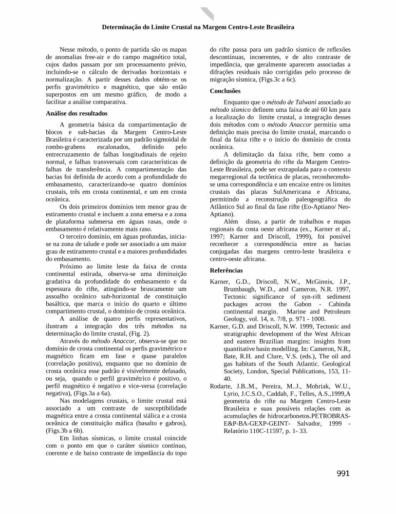
Determinação do Limite Crustal na Margem Centro-Leste Brasileira

Nesse método, o ponto de partida são os mapas de anomalias free-air e do campo magnético total, cujos dados passam por um processamento prévio, incluindo-se o cálculo de derivadas horizontais e normalização. A partir desses dados obtém-se os perfis gravimétrico e magnético, que são então superpostos em um mesmo gráfico, de modo a facilitar a análise comparativa.

Análise dos resultados

A geometria básica da compartimentação de blocos e sub-bacias da Margem Centro-Leste Brasileira é caracterizada por um padrão sigmoidal de rombo-grabens escalonados, definido pelo entrecruzamento de falhas longitudinais de rejeito normal, e falhas transversais com características de falhas de transferência. A compartimentação das bacias foi definida de acordo com a profundidade do embasamento, caracterizando-se quatro domínios crustais, três em crosta continental, e um em crosta oceânica.

Os dois primeiros domínios tem menor grau de estiramento crustal e incluem a zona emersa e a zona de plataforma submersa em águas rasas, onde o embasamento é relativamente mais raso.

O terceiro domínio, em águas profundas, inicia-se na zona de talude e pode ser associado a um maior grau de estiramento crustal e a maiores profundidades do embasamento.

Próximo ao limite leste da faixa de crosta continental estirada, observa-se uma diminuição gradativa da profundidade do embasamento e da espessura do rifte, atingindo-se bruscamente um assoalho oceânico sub-horizontal de constituição basáltica, que marca o início do quarto e último compartimento crustal, o domínio de crosta oceânica.

A análise de quatro perfis representativos, ilustram a integração dos três métodos na determinação do limite crustal, (Fig. 2).

Através do método Anaccor, observa-se que no domínio de crosta continental os perfis gravimétrico e magnético ficam em fase e quase paralelos (correlação positiva), enquanto que no domínio de crosta oceânica esse padrão é visivelmente defasado, ou seja, quando o perfil gravimétrico é positivo, o perfil magnético é negativo e vice-versa (correlação negativa), (Figs.3a a 6a).

Nas modelagens crustais, o limite crustal está associado a um contraste de susceptibilidade magnética entre a crosta continental siálica e a crosta oceânica de constituição máfica (basalto e gabros), (Figs.3b a 6b).

Em linhas sísmicas, o limite crustal coincide com o ponto em que o caráter sísmico contínuo, coerente e de baixo contraste de impedância do topo

do rifte passa para um padrão sísmico de reflexões descontínuas, incoerentes, e de alto contraste de impedância, que geralmente aparecem associadas a difrações residuais não corrigidas pelo processo de migração sísmica, (Figs.3c a 6c).

Conclusões

Enquanto que o método de Talwani associado ao método sísmico definem uma faixa de até 60 km para a localização do limite crustal, a integração desses dois métodos com o método Anaccor permitiu uma definição mais precisa do limite crustal, marcando o final da faixa rifte e o início do domínio de crosta oceânica.

A delimitação da faixa rifte, bem como a definição da geometria do rifte da Margem Centro-Leste Brasileira, pode ser extrapolada para o contexto megarregional da tectônica de placas, reconhecendo-se uma correspondência e um encaixe entre os limites crustais das placas SulAmericana e Africana, permitindo a reconstrução paleogeográfica do Atlântico Sul ao final da fase rifte (Eo-Aptiano/ Neo-Aptiano).

Além disso, a partir de trabalhos e mapas regionais da costa oeste africana (ex., Karner et al., 1997; Karner and Driscoll, 1999), foi possível reconhecer a correspondência entre as bacias conjugadas das margens centro-leste brasileira e centro-oeste africana.

Referências

Karner, G.D., Driscoll, N.W., McGinnis, J.P., Brumbaugh, W.D., and Cameron, N.R. 1997, Tectonic significance of syn-rift sediment packages across the Gabon - Cabinda continental margin. Marine and Petroleum Geology, vol. 14, n. 7/8, p. 971 - 1000.

Karner, G.D. and Driscoll, N.W. 1999, Tectonic and stratigraphic development of the West African and eastern Brazilian margins: insights from quantitative basin modelling. In: Cameron, N.R., Bate, R.H. and Clure, V.S. (eds.), The oil and gas habitats of the South Atlantic. Geological Society, London, Special Publications, 153, 11-40.

Rodarte, J.B..M., Pereira, M..J., Mohriak, W.U., Lyrio, J.C.S.O., Caddah, F., Telles, A.S.,1999,A geometria do rifte na Margem Centro-Leste Brasileira e suas possíveis relações com as acumulações de hidrocarbonetos.PETROBRAS-E&P-BA-GEXP-GEINT- Salvador, 1999 - Relatório 110C-11597, p. 1- 33.

Determinação do Limite Crustal na Margem Centro-Leste Brasileira

Determinação do Limite Crustal na Margem Centro-Leste Brasileira

EL “HOYO DE OROCUAL” … UNACURIOSIDAD GEOLOGICA, IMPACTODE METEORITO o ESTRUCTURA DECOLAPSO.Gilberto Parra, PDVSA, parragi@pdvsa.comPedro Villarroel, PDVSA, villarroelp@pdvsa.comJuan Guevara, PDVSA, guevarajq@pdvsa.comGustavo Carvajal, PDVSA, carvajalge@pdvsa.com

RESUMEN:

El “hoyo de Orocual” es una curiosa estructurageológica, la cual ha sido objeto de numerosasinterpretaciones a lo largo de la historia del campo, seencuentra ubicado al norte del edo. Monagas, al estede Venezuela, figura N° 1.En este trabajo presentaremos todas las teorías quehan tratado de explicar el origen de “Hoyo”, lamayoría se refiere a una estructura de colapsoasociado a los corrimientos del frente de deformacióny al diapirismo de lodo característico del norte demonagas, figura N° 2,sin embargo existe un buennúmero de geólogos que piensan que puede tratarsedel impacto de un meteorito, y considerando queexisten unos quince campos petroleros asociados aimpactos de meteoritos la idea no es ilógica. PDVSAExploración y Producción, por medio de la Unidad deExplotación Norte asumió a finales de 1997, lagerencia del viejo campo Orocual somero, el mismoestá localizado en el norte del estado Monagas, al surdel cinturón plegado conocido como la Serranía delInterior, con la finalidad de buscar nuevasoportunidades que permitan incrementar laproducción, se conformó un equipomultidisciplinario, combinando la geociencia, elconocimiento de la ingeniería de reservorio y deproducción, utilizando nuevas tecnologías deperforación y rehabilitación, basado en la revisión dela poca información dinámica y estática disponible.Como parte de estas actividades, y para hacer a unmodelo sísmico estructural del área, se llevó a cabo lainterpretación sísmica 3D, con 200 Km2 deinformación sísmica del proyecto OROCUAL-93,diseñado para objetivos profundos. El levantamientode OROCUAL-93 cubre el 100% del área de estudioy los pozos perforados se ubican dentro de suslímites. Para la interpretación se utilizó una versiónreprocesada a fase cero y amplitud preservada porconsiderarse que es de mejor calidad que la versiónoriginal. El levantamiento OROCUAL-93, conformado por1300 líneas orientadas NW-SE y 700 trazasorientadas SW-NE, cubre un área de 200 Km2

interpretados totalmente en cuanto a pozos se refiere,

se utilizaron los datos de 110 pozos. En el áreaexisten 14 pozos con datos de velocidad quepermitieron calibrar la sísmica con los pozos, serealizaron los sismogramas sintéticos de estos 14pozos. DESCRIPCIÓN:

Se interpretaron cinco marcadores sísmicos regionalespara un mejor control de la estructura, en la cual cabedestacar la presencia de una depresión de casi 3 Kmsde diámetro y 4000 pies (1200 metros) de calidad,dentro de esta estructura la acumulación está encompartimientos estructurales, cuya prospectividadradica en que dentro de la misma se acumulanhidrocarburos livianos, medianos, fuera de este“hoyo” la acumulación es de crudo pesado, al lado deesta estructura se encuentra un anticlinal el cual estágenéticamente relacionado con el “hoyo”, ver figuraN° 3.Las fallas se comenzaron a interpretar en formaparalela a la sedimentación al este de la zona deestudio en virtud de que la mayoría de las fallas sonde tipo normal y buzan al sur con dirección SW-NE,al oeste del área de estudio la dirección del sistema defallas se orienta NW-SE, son normales y buzan aloeste, razón por la cual las líneas se interpretaronperpendicular a la dirección de la sedimentación. Enla zona de la estructura de colapso se interpretó tantoen las “inlines” como en las “crosslines”, además delíneas arbitrarias para la definición de las fallas, en sumayoría normales. La generación de seccioneshorizontales constituyeron una herramientafundamental en la comprensión del sistema de fallas,pero muy en particular en la zona del colapso. Lainterpretación y animación sísmica con el módulo deSeiscube fue muy útil familiarizarse con el sistema delas fallas. Casi simultáneamente con la interpretaciónse triangularon e interpolaron los segmentos de lasfallas de interés, para la posterior generación de lospolígonos de fallas y validación de los planos conrespecto a pozos fallados.En el área de Orocual existen 14 pozos profundos ydos someros con datos de velocidad. Estos datosfueron cargados en la aplicación SEISWORKTM de lacompañía LANDMARK GRAPHICS Co. en laelaboración de sismogramas sintéticos y el modelo develocidad, se calcularon los pares tiempo-profundidad, valores de velocidad promedio yvelocidad interválica calculadas a partir de losmismos así como sus respectivos gráficos.Para realizar la calibración pozo-sísmica se generaron14 sismogramas sintéticos. La calibración sísmica-pozo es en general de buena calidad. Se debe

EL “HOYO DE OROCUAL”mencionar que en ciertos casos se aplicó undesplazamiento “shift” a las curvas de velocidad amanera de asegurar una correlación adecuada con lasísmica.

RESULTADOS:

La calidad de los datos para la Formación LasPiedras puede ser subdividida en tres áreasprincipales:En el Área del diapiro, la calidad de la sísmica es deregular a buena los reflectores son relativamentefuertes y muestran buena continuidad lateral,facilitando la cartografía y delineado del diapiro. Eldiapirismo fracturó completamente los estratossuperiores, y ocasionó un extenso fallamiento en sutope, aunque lateralmente las reflexiones muestrancontinuidad y son cartografiables.El Área Norte, presenta una calidad de datos deregular resolución lateral en la zona productora. En el Área de la Estructura de Colapso, por la propianaturaleza la masa homogénea prácticamente noofrece contraste de impedancia acústica, enconsecuencia no hay reflexiones, en gran parte de laestructura de colapso no es posible seguir reflectoralguno, ya que la señal sísmica está altamenteperturbada, ningún reprocesamiento podría mejoraresta situación. El área del hoyo va disminuyendo conla profundidad, mejorando ligeramente la resoluciónlateral. Se interpretó la estructura la cual correspondea un monoclinal con buzamiento promedio 10° alsureste, alterado por un hoyo y un anticlinalorientados en sentido SSW-NNE, figura N° 4. En la línea de trabajo que hemos seguido, seanalizaron varios modelos estructurales que podríanexplicar la formación de la estructura de colapso y elanticlinal como consecuencia del diapirismo de lodo,el modelo propuesto – sin pretender tener la últimapalabra - consiste en un sistema de fallas tipo “cola decaballo” sensu lato, estos sistemas fueron muy biendescritos por Chinnery, 1966, ver figura N° 5.Los segmentos de fallas en colores ocre, amarillo,fucsia, naranja, verde, amarillo y marrón claro,corresponden al sistema principal de transcurrencia,la respuesta sísmica de forma elipsoidal indica lapresencia del anticlinal producto del diapiro de lodo.Las fallas representadas en color amarillo se insinúanen las secciones horizontales, en las seccionesverticales es prácticamente imposible observarlas,este patrón es característico de las fallas asociadas lafalla transcurrente principal, las orientadas en sentidoNO-SE, corresponderían al patrón tipo riedel (Rshears), las fallas orientadas en sentido NE-SOpodrían corresponder a los patrones R’ shear y/o Pshear.

En la zona oeste del área de estudio se aprecia unpatrón de fallas con orientación preferencial norte-sur, las mismas son de carácter normal, conevidencia de rotación entre los bloques a amboslados de las fallas, las mismas presentan unaseparación vertical estimada de 50 a 80 pies. Esterasgo estructural tiene similitud con el modelo deChinnery, 1966, correspondiente al Tipo B.La estructura de colapso de Orocual corresponde auna depresión de forma elipsoidal, su eje más largode 1500 m aprox., en sentido SO-NE, es decir, con lamisma dirección del diapiro, su eje corto seencuentra en dirección casi perpendicular al ejeprincipal., El diámetro promedio es de 3 kms, con undesnivel de 4200 pies(1280 m). La parte másprofunda del hoyo está ubicada al norte, el pozoORS-21 penetró el tope de la Fm. Carapita @ 7631’.

Su peculiar fallamiento puede subdividirse endos patrones, un patrón de fallas concéntricassubverticales de carácter normal, con saltos verticalesque van desde 100 pies y hacia el norte del hoyopueden superar los 2000 pies. El otro sistema de fallases pseudoradial, también fallas subverticales,normales, generandose una gran cantidad decompartimientos estructurales, donde prácticamentecada pozo está en un bloque. De este segundo patrónde fallas destaca la falla color morado la cual reflejaun movimiento de transcurrencia dextral. El rango debuzamiento de las capas se encuentra en el orden delos 14°-54°, hacia el borde del hoyo se presentan losbuzamientos más elevados, y sísmicamente todavía seobserva buena señal. La cartografía dentro del hoyose apalancó en el número de pozos concentrados en elhoyo, datos de buzamientos, datos de producción,secciones sísmicas horizontales y verticales.El trabajo siguiente será la restauración y balanceo desecciones a fin de descartar inconsistencias en lainterpretación.Sin embargo existen rasgos morfológicos del “hoyo”que se insinúan como un cráter producto del impactode meteorito teoría que aún no ha sido losuficientemente defendida.(Figura N° 6).

CATEGORÍA TÉCNICA:

INTERPRETACIÓN SÍSMICA.

EL “HOYO DE OROCUAL” FIGURA N° 1 Mapa de ubicación.

FIGURA N° 2 Corte esquemático del campo.

FIGURA N° 3 Time slice mostrando el hoyo y el diapiro.

FIGURA N° 4 Modelo estructural interpretado.

FIGURA N° 5 Modelo básico de Chinnery, 1966.

OROCUAL

2

4 Kms

6

PPIIRRIITTAALL TTHHRRUUSSTT

OORROOCCUUAALL TTHHRRUUSSTT

V=HOriginal by Flinch, J., 1997

HOYO OROCUALLLAASS PPIIEEDDRRAASS FFMM..

“HOYO”

DIAPIRO

MONOCLINAL

HOYO

DIAPIRO

SINCLINAL

Z.P.

Zona elevadapor compresión

Zona deprimida

Zona Principal deDesplazamiento

EL “HOYO DE OROCUAL”FIGURA N° 6 Teoría del impacto y su posible

Trayectoria

DIRECCION DEL IMPACTO

Growth Folding in Gravitational Fold-and-Thrust Belts in the Deep Waters of the Equatorial Atlantic, Northeastern Brazil Pedro Victor Zalán, PETROBRAS S/A, Brazil Introduction As the continental margins build outward into deep and ultra-deep waters via continuous denudation of the adjoining shields and sedimentation of the debris forming the continental shelves and slopes, the rifted/thinned edge of the continental plates cool exponentially as they move away from the heat source that created the rupture and breaking of the former larger continental plate. These create a very unstable situation since large volumes of sediments pile up at the margin of the continental shelves, in the upper slope, at the same time the whole area is gradually tilting oceanward due to thermal flexural bending. Gravity failure occurs and allochtonous masses of sediments slide down the slope, over a plastic lithology that acts as a lubricant and detaches the traveling rocks above from the autochtonous rocks below. When the frontal parts of the allochton diminish their velocity due either to a decrease in the gradient of such detachment zone or to a physical barrier (commonly a volcanic edifice) the incoming allochtons collide and strong contraction/compression occurs.

The failure occurs when vertical stresses due to overburden are weakened in relation to sub-horizontal stresses due to several possibilities, including overpressure in shales (due to petroleum generation or any other classical overpressure mechanism) or ductile flow in salt. Shear stresses develop parallel to the slightly dipping bedding and overcome the vertical stresses These deformed masses of allochtonous rocks are nowadays referred to as linked extensional-compressional systems and have been found in the deep/ultra-deep water regions of most continental margins around the world. It is easily understood, and very well displayed in modern seismic sections, that these systems are composed of three major tectonic domains, each one presenting different and peculiar deformation (Figure 1). The extensional domain comprises highly strained subsided terrains at the upper continental slope, dominated by arcuated listric normal faults that sole out at the detachment level. Major listric faults present significant associated rollover anticlines and growth depositional wedges that thicken from the crest of the anticline towards the listric fault. Subsidiary listric normal faults, antithetic to the major downdip listric faults, are also abundant, as well as crestal fracturing/faulting in the rollover anticlines.

The translational domain is a predominantly non-deformed region, that passively traveled over the detachment zone. Weak arching may affect the rocks present in this area. The compressional domain may present spectacular deformation, with all kinds of reverse and thrust faults and fault-related folding (detachment, fault-propagation and fault-bend folding). When detached on shales, the structural styles and dimensions may resemble those found in truly orogenic belts (Zalán 1998). When salt is the lubricant, deformation is more complex and salt canopies develop. The specific name gravitational fold-and-thrust belts (GFTB’s) have been applied to such entities. Zalán (1999) studied some brazilian GFTB’s in detail and devised a tripartite structural model that predicts an orderly succession, from the internides to the foreland, of detachment folding, followed by high-angle reverse faults and associated fault-propagation folds, ending in low angle, ramp-flat thrusts with associated fault-bend folding. Important oil discoveries have been achieved in these compressional provinces in deep waters off Nigeria Angola, GOM and Brazil. The dimensions of these three domains may vary greatly. Usually the extensional and compressional domains are the widest but it is very difficult to exactly balance the amount of extension updip with the amount of contraction downdip, because of the details of the severe deformation that is usually non-resolvable by the volumes of seismic data available. Since they cover huge areas, in the order of several thousand square kilometers, it is difficult to have them all covered by 3D seismic, and it is not unusual that extension and compression be divided into two or three belts of deformation. GFTB’s with Growth Folding When the process of gravity sliding/contraction is long-lasting (10-40 m.y.) and takes place in areas with low rates of sedimentation the peculiar mechanism of growth folding comes into scene. Since GFTB’s develop in exclusively submarine environments, they are never subaerially exposed, sedimentation takes place concomitantly with the compressional deformation leading to the deposition of syntectonic growth strata that thin up onto the upper parts of the foldbelt, in the same way the growth wedges develop in the downthrown sides of the normal faults in the extensional domains.

Medwedeff (1989) unraveled complex growth stratigraphic relationships between coeval sediments deposited in the forelimb and back-limb of a single fault-bend fold in California. Numerous wells and seismic data allowed the author to deduce that syntectonic sedimentary strata onlap a time-transgressive unconformity on the forelimb but have uniform dip and constant thickness, and are folded below the unconformity on the back-limb (Figure 2).

Same age sediments are deposited over the positive topographic expression of the fold (forelimb) in onlap pattern, as well as conformably over the horizontal strata that is traveling towards the deformation locus (back-limb). These horizontal strata have constant thickness and are rolled through an active axial surface forming the back-limb of the fold that will continuously grow towards the internal part of the deformation, while the forelimb will be passively transported in the other direction towards the foreland. A time-transgressive unconformity continuously develops in the same direction as the fold grows, toward the internides, and erodes/covers the sediments that are folded and uplifted in the back-limb.

The same mechanism seems to be applicable to GFTB’s in the Brazilian equatorial atlantic margin, such as the Pará-Maranhão, Barreirinhas and Touros GFTB’s. Figure 3 shows an interpreted depth seismic section from the Pará-Maranhão Basin, where three reflectors can be correlated across four time-transgressive unconformities (dark yellow). These reflectors (dark green, purple and blue) are interpreted to encompass the growth strata associated to this GFTB. The geometry of the deformation in this GFTB suggests that the folding and uplift of the thrust strata was a long-lived process. Since there is a major long-lasting time-transgressive unconformity (as well as three minor ones) that separates the non-deformed strata above from the deformed strata below it is plausible to deduce that the rates of sedimentation were low, the uplifted/folded/thrust strata was left exposed at the sea bottom and submarine erosion (currents) could take place. The same pattern of a series of younging- and stepping-upward time-transgressive unconformities separating non-deformed onlapping strata above from thrust and folded strata below can be seen in several other GFTB’s in Brazil (Barreirinhas and Touros) and elsewhere in the world (for instance, in the Krishna-Godavari Basin, in India) and are here interpreted as being diagnostic of gravity sliding/contraction accompanied by growth folding in areas dominated by low rates of deformation and sedimentation.

GFTB’s without Growth Folding Some GFTB’s do not display the complicated pattern of time-transgressive unconformities as described above. They involve thick packages of sediments that are folded and thrust harmonically. Syntectonic sedimentation seems to follow a simpler and more easily understood pattern of being confined to intervening synclines between anticlines. In this case, the syncline packages typically thicken downward towards the depocenter and thin upward towards the anticlines. Such is the case in the Foz do Amazonas (Figure 4), Cone do Rio Grande and Niger delta GFTB’s, where all allochtonous sediments are harmonically folded and thrust up into the sea bottom. They are situated in front of young deltas (Miocene) where huge piles of sediments accumulated very quickly in a very short time, while gravity sliding was taking place, also during the same short time. The pattern of harmonically folded and thrust sediments, with thick syntectonic packages in the synclines and thinner correlative packages on the anticlines, and more importantly, the absence of time-transgressive unconformities, are here interpreted as being diagnostic of gravity sliding/contraction in areas dominated by high rates of deformation and sedimentation. The major implications for such differences in the depositional/structural styles of the growth strata are in the location of the turbidite beds and the related hydrocarbon traps. References Medwedeff, D.A., 1989, Growth fault-bend folding at

southeast Lost Hills, San Joaquin Valley, California: AAPG Bulletin, v.73, p. 54-67.

Zalán, P. V., 1998, Gravity-driven compressional structural closures in Brazilian deep-waters: a new frontier play: AAPG Annual Meeting Extended Abstracts vol. 2, Salt Lake City, Utah, p. A723.

Zalán, P.V., 1999, Seismic expression and internal order of gravitational fold-and-thrust belts in Brazilian Deep Waters (expanded abstract): Sixth International Congress of the Brazilian Geophysical Society, CD-ROM with Extended abstracts, Rio de Janeiro, August, 4 p.

Zalán, P.V., 2001, Growth Folding in Gravitational Fold-and-Thrust Belts in the Deep Waters of the Equatorial Atlantic, Northeastern Brazil: AAPG Annual Convention Official Program Book and CD-ROM, Denver, June, p. A223.

Figure 1 – Linked extensional-compressional systems (linkage via detachment surface) consist of three major tectonic domains: extensional, translational and compressional, each with their own specific structural style. The compressional domain is usually called gravitational fold-and-thrust belts (GFTB’s) and the style here illustrated depicts the situation of a non-mobile shale-cored detachment zone. When the GFTB is cored in mobile plastic lithologies such as salt, or even shale, more complex deformation is created (diapirs, salt canopies, disharmonic folding)

Figure 2 – Growth folding mechanism devised by Medwedeff (1989) for a fault-bend fold in California.

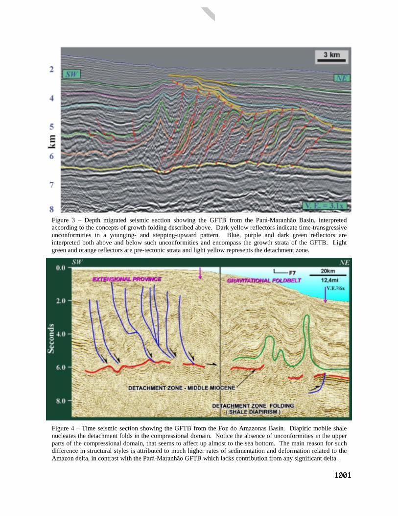
Figure 3 – Depth migrated seismic section showing the GFTB from the Pará-Maranhão Basin, interpreted according to the concepts of growth folding described above. Dark yellow reflectors indicate time-transgressive unconformities in a younging- and stepping-upward pattern. Blue, purple and dark green reflectors are interpreted both above and below such unconformities and encompass the growth strata of the GFTB. Light green and orange reflectors are pre-tectonic strata and light yellow represents the detachment zone.

Figure 4 – Time seismic section showing the GFTB from the Foz do Amazonas Basin. Diapiric mobile shale nucleates the detachment folds in the compressional domain. Notice the absence of unconformities in the upper parts of the compressional domain, that seems to affect up almost to the sea bottom. The main reason for such difference in structural styles is attributed to much higher rates of sedimentation and deformation related to the Amazon delta, in contrast with the Pará-Maranhão GFTB which lacks contribution from any significant delta.

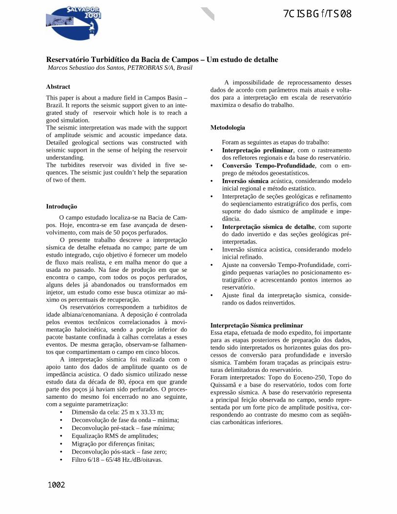
Reservatório Turbidítico da Bacia de Campos – Um estudo de detalhe Marcos Sebastiao dos Santos, PETROBRAS S/A, Brasil

Abstract

This paper is about a madure field in Campos Basin –Brazil. It reports the seismic support given to an inte-grated study of reservoir which hole is to reach agood simulation.The seismic interpretation was made with the supportof amplitude seismic and acoustic impedance data.Detailed geological sections was constructed withseismic support in the sense of helping the reservoirunderstanding.The turbidites reservoir was divided in five se-quences. The seismic just couldn’t help the separationof two of them.

Introdução

O campo estudado localiza-se na Bacia de Cam-pos. Hoje, encontra-se em fase avançada de desen-volvimento, com mais de 50 poços perfurados.

O presente trabalho descreve a interpretaçãosísmica de detalhe efetuada no campo; parte de umestudo integrado, cujo objetivo é fornecer um modelode fluxo mais realista, e em malha menor do que ausada no passado. Na fase de produção em que seencontra o campo, com todos os poços perfurados,alguns deles já abandonados ou transformados eminjetor, um estudo como esse busca otimizar ao má-ximo os percentuais de recuperação.

Os reservatórios correspondem a turbiditos deidade albiana/cenomaniana. A deposição é controladapelos eventos tectônicos correlacionados à movi-mentação halocinética, sendo a porção inferior dopacote bastante confinada à calhas correlatas a esseseventos. De mesma geração, observam-se falhamen-tos que compartimentam o campo em cinco blocos.

A interpretação sísmica foi realizada com oapoio tanto dos dados de amplitude quanto os deimpedância acústica. O dado sísmico utilizado nesseestudo data da década de 80, época em que grandeparte dos poços já haviam sido perfurados. O proces-samento do mesmo foi encerrado no ano seguinte,com a seguinte parametrização:

• Dimensão da cela: 25 m x 33.33 m;• Deconvolução de fase da onda – mínima;• Deconvolução pré-stack – fase mínima;• Equalização RMS de amplitudes;• Migração por diferenças finitas;• Deconvolução pós-stack – fase zero;• Filtro 6/18 – 65/48 Hz./dB/oitavas.

A impossibilidade de reprocessamento dessesdados de acordo com parâmetros mais atuais e volta-dos para a interpretação em escala de reservatóriomaximiza o desafio do trabalho.

Metodologia

Foram as seguintes as etapas do trabalho:• Interpretação preliminar, com o rastreamento

dos refletores regionais e da base do reservatório.• Conversão Tempo-Profundidade, com o em-

prego de métodos geoestatísticos.• Inversão sísmica acústica, considerando modelo

inicial regional e método estatístico.• Interpretação de seções geológicas e refinamento

do seqüenciamento estratigráfico dos perfis, comsuporte do dado sísmico de amplitude e impe-dância.

• Interpretação sísmica de detalhe, com suportedo dado invertido e das seções geológicas pré-interpretadas.

• Inversão sísmica acústica, considerando modeloinicial refinado.

• Ajuste na conversão Tempo-Profundidade, corri-gindo pequenas variações no posicionamento es-tratigráfico e acrescentando pontos internos aoreservatório.

• Ajuste final da interpretação sísmica, conside-rando os dados reinvertidos.

Interpretação Sísmica preliminarEssa etapa, efetuada de modo expedito, foi importantepara as etapas posteriores de preparação dos dados,tendo sido interpretados os horizontes guias dos pro-cessos de conversão para profundidade e inversãosísmica. Também foram traçadas as principais estru-turas delimitadoras do reservatório.Foram interpretados: Topo do Eoceno-250, Topo doQuissamã e a base do reservatório, todos com forteexpressão sísmica. A base do reservatório representaa principal feição observada no campo, sendo repre-sentada por um forte pico de amplitude positiva, cor-respondendo ao contraste do mesmo com as seqüên-cias carbonáticas inferiores.

Reservatório Turbidítico da Bacia de Campos – Um estudo de detalhe

Figura 1 – Seção sísmica em tempo. Notar refleto-res regionais e falhas delimitadoras. Reservatóriorepresentado por anomalia branca na seção.

Conversão Tempo-Profundidade

O modelo de velocidade empregado na conversão foicalculado com o emprego de métodos geoestatísticos,consistindo em uma Krigagem com deriva externaentre os pontos de amarração sísmica (em tempo) eperfis (em profundidade).A deriva externa foi definida a partir dos dados deperfis sônicos, devido à inexistência dos arquivos deanálise de velocidade. Foram utilizados os horizontesregionais para guiar a interpolação.

Inversão Sísmica

A obtenção do modelo ótimo de impedancia acústicadeu-se com o emprego de procedimento com formu-lação baysiana, no qual os dados de amplitude sãoajustados a um modelo de impedância acústica inicial,gerado a partir de informações derivadas de poços edo conhecimento geológico prévio.

As etapas desse procedimento podem ser agrupadasem:• Determinação da wavelet (integração perfil-

sísmica).Foi considerado como o melhor ajuste, uma wa-velet de fase zero, de comprimento igual a 204ms, correspondendo a um filtro de Hanning, comfreqüência de corte 0-8/40-60 Hz.

• Geração do modelo a priori (condicionamentoinicial da inversão).Foram utilizados 18 poços, representando todosaqueles com perfil sônico na área de estudo.O modelo da primeira inversão efetuada conside-rou como condicionantes a Base das areias e o

topo do Eoceno-250. Já para a segunda inversão,a esses dois horizontes somaram-se o topo da Se-qüência 1 e o topo do Cenomaniano-150 (Figura2).

• Inversão propriamente dita.

Figura 2 – Modelo geológico da Inversão II

Estratigrafia/ Modelo Deposicional e Interpreta-ção Sísmica de Detalhe

No modelo estratigráfico estabelecido para o reser-vatório foram definidas duas seqüências de terceiraordem, sendo a inferior dividida em três subseqüên-cias de quarta ordem (seqüências 0, 1 e 2) e a superiorem duas ( seqüências 3 e 4).Os eventos de terceira ordem são controlados pormovimentação tectônica, principalmente halocinese eeustasia. O primeiro evento, com cerca de 4 ma edatado do Albiano superior, está depositado sobreseqüência carbonática, em calhas criadas, principal-mente, pela a ação da tectônica do sal.O segundo evento, de idade Cenomaniano médio, foidepositado em um periodo pouco maior que 4 ma deanos, após um hiato de 2.4 ma, reconhecido em se-ções sísmicas, análises bioestratigráficas e perfis depoços. Comparativamente ao evento sotoposto, possuicaráter menos confinado.Do ponto de vista deposicional, as cinco seqüênciasde quarta ordem podem ser agrupadas em três siste-mas turbidíticos distintos.O primeiro envolve a Seqüência 0, que representa aporção mais basal do reservatório. A deposição dessaé relevante apenas na porção S/SE do campo, possu-indo forte controle tectônico. Os sedimentos dessasão constituídos, em sua maior parte, por depósitos deescorregamento e fluxo de detritos, além de isoladosdepósitos turbidíticos confinados.Como pode ser visto nos histogramas da figura 3,comparativamente às seqüências superiores, a Se-qüência 0 possui valores de impedância mais eleva-

Reservatório Turbidítico da Bacia de Campos – Um estudo de detalhedos, correlatos às fácies não reservatório. No dadosísmico esse contraste é bem pronunciado, o quefacilitou o mapeamento do topo dessa seqüência. Afigura 4 apresenta o mapa de espessura sísmica dessaunidade,.

Figura 3 – Histograma de impedâncias das se-qüências 0, 1 e 2. Notar a boa discriminação daSeqüência 0, em relação às superiores.

Figura 4 – Mapa de espessura sísmica da Seqüên-cia 0. Notar forte controle estrutural.

O segundo sistema turbidítico engloba as seqüências1 e 2. O controle tectônico continua a ser preponde-rante na geração de espaços para a deposição, princi-palmente na criação de uma calha contínua, onde sedeposita a Seqüência 1 (Figura 5). A Seqüência 2 édepositada em duas calhas menores (Figura 6). Aseparação entre essas duas seqüências é possíveldevido ao comportamento sísmico da zona de con-densação do topo da Seqüência 1, posicionada empico de amplitude positiva.

No dado sísmico de amplitude não existem feiçõesque possibilitem o rastreamento do topo da Seqüência2. No entanto, apesar da pequena diferença entre osvalores de impedância dessa seqüência e os da Se-qüência 3 (Figura 7), foi possível a interpretaçãonesse tipo de dado, uma vez que as feições geométri-cas observadas mostram coerência com os marcosestratigráficos observados em perfil.

Figura 5 – Mapa de espessura sísmicada Seqüên-cia 1. Notar deposição confinada à calha principal.

Figura 6 – Mapa de espessura sísmica da Seqüên-cia 2.

O terceiro sistema turbidítico engloba as seqüências 3e 4. O hiato erosivo entre esse sistema e o sotoposto,de pequena expressão no dado de amplitude sísmica,é corretamente identificado no dado invertido paraimpedância acústica, onde são observadas as estrutu-ras se interrompendo na discordância entre os doissistemas (Figura 8).

Reservatório Turbidítico da Bacia de Campos – Um estudo de detalhe

Figura 7 - Histograma de impedâncias das seqüên-cias 2, 3 e 4.

Figura 8 – Seção em impedância acústica. Notar asfeições geométricas contra o refletor assinalado –Topo da Seqüência 2).

As seqüências desse terceiro sistema são depositadasde maneira mais espraiada. A inexistência de umazona de condensação pronunciada no topo da Se-qüência 3, além do posicionamento das impedânciasdas duas seqüências na mesma faixa de valores,impede a compartimentação desse sistema com basedo dado sísmico (Figura 9).O pacote é recoberto por um espesso pacote de lami-tos radioativos, identificados na sísmica, e que repre-sentam o topo do reservatório.

Conclusões

A base de dados sísmicos utilizados, adquirida há 15anos e impossibilitada de ser reprocessada, pode servista com um fator limitante de qualidade no presentetrabalho. Algoritmos mais recentes de processamento,que buscam uma maior acurácia na preservação dasamplitudes sísmicas, certamente gerariam uma maiorconfiança nestes como dado de entrada para os apli-cativos de inversão estratigráfica. Do mesmo modo,uma maior resolução na aquisição dos dados ocasio-

naria uma maior definição das feições internas aocampo.

Figura 9 – Mapa de espessura sísmica das seqüên-cias 3 e 4. Notar o maior espraiamento do reserva-tório.

A metodologia aplicada na conversão tempo–profun-didade foi idealizada durante a realização do projeto,visando contornar a inexistência de dados de análisede velocidade de empilhamento nos bancos de dadosda companhia e, pelos resultados apresentados, pode-rá ser aplicada em situações similares.A interpretação dos limites do reservatório foi efe-tuada, de maneira satisfatória, tendo como base odado de amplitude sísmica, no entanto, algumas dasseqüências internas desse, que tiveram seu posi-cionamento balizado pelos dados de bioestratigrafia,só puderam ser definidas na sísmica baseadas naimpedância.

Referências Bibliográficas-

Johann, P., 1997, Inversion Sismostratigraphique etSimulations Stochastiques em 3D: Réservoir Tur-biditique, offshore du Brésil. Intègration Geólogi-que, Géophysique et Géostatistique. Tese de dou-torado, 351 pp.

Schwedersky, G., Mundim, E.C. e Johann, P, 1999,Inversão Sísmica na Caracterização de Reservató-rio. Relatório Interno, Petrobras, 65 pp.

Mundim, E.C., 2000, Conversão Tempo- Profundida-de. Relatório interno – Petrobras, 49 pp.

Agradecimentos

Agradeço à Petrobras por permitir a publicação dessetrabalho e também aos geólogos Rosane Trajano,Eduardo Rodrigues, Viviane Santos e OscarStrohschoen pela definição de todo o arcabouço geo-lógico, base para esse trabalho. Agradeço também aosgeofísicos Paulo Johann, e Evaldo Mundim pelopioneirismo e apoio nos procedimentos aqui relata-dos.

Sedimentary facies mapping based on bottom surface backscattering strengthMaria Gilda P. Esteves LAGEMAR-UFF, Brazil (gilda@igeo.uff.br); Alberto G. Figueiredo Jr. LAGEMAR-UFF,Brazil (alberto@igeo.uff.br) and Letícia R. de Carvalho FURG, Brazil (doclrc@super.furg.br)

Abstract

Bottom surface backscattering strength (BSBS) datafrom southern Brazilian shelf and slope, betweenCape São Tomé and Arroio Chuí were used to char-acterize bottom sediment from 50 to 1,500 m waterdepths as part of the Brazilian national program enti-tled "Sustainable Potential of Living Resources of theEconomic Exclusive Zone" (REVIZEE). The BSBSdata is compared to 3,036 bottom samples and resultsallowed bottom sediment classification accordinglyacoustic characteristics and grain-size.

IntroductionMapping of sedimentary facies and depositional pro-cesses at the ocean bottom based on response to echosounders (echo character) have been applied by Da-muth (1975), Mullins et al. (1979), Flood (1980),Costa (1997) and Costa & Figueiredo Jr. (1998). Andsince development of digital technique for storingecho sounder data, it has been possible to associatelevel of acoustic impedance to sediment facies. Thistechnique was applied to an area of the Braziliancontinental shelf and slope between Cape São Toméand Arroio Chuí in an extension of 2,400 km in waterdepths ranging from 50 to 1500m. This mapping wasdeveloped as part of a Brazilian national programentitled "Sustainable Potential of Living Resources ofthe Economic Exclusive Zone" (REVIZEE) on boardof RV Atlântico Sul from Fundação UniversidadeFederal do Rio Grande (FURG).The authors are aware of software packages able toused BSBS to classify ocean bottom sediment, how-ever due to high commercial costs of packages andpossibility of development of the technique inhouse,we decide to write this paper.

The Data Set

The acoustic data were collected with a Simrad EK500 echosounder operating in a frequency of 38 kHz.The data used is one of the acoustic measurementsprovided by the echosounder telegram called "bottomsurface backscattering strength (BSBS). The valuesare furnished in decibel and were collected in a rate of9 to 12 values per minute with ship sailing at 10knots.Bottom sample data are from 3,036 samples from theBrazilian Program in Marine Geology and Geophys-ics (PGGM) Data Bank, from the Brazilian Margin

Reconnaissance Program (REMAC) and REVIZEEProgram.

Bottom Classification ProcedureIn order to proceed with sediment classification, ini-tially the sediment samples have to be classified ac-cordingly to Shepard (1954) triangular diagram ofproportional mixing of sediment types (Fig. 1).Next, sample class is compared to BSBS values hav-ing as common data the geographical coordinates.For sediments in the extreme of the classificationdiagram, BSBS values are well defined, but in manycases of sediment mix, BSBS values could corre-spond to more than one sediment class. In these cases,decision has to be taken, based on statistical occur-rence and better fitting of the data.Results can be used as bulk values of decibel X sedi-ment class or transformed into maps were areas ofsame BSBS values are contoured.

Figure 1 –triangular diagram of mix proportion ofsediment. (After Shepard, 1954)

Results

Correlation of sediment class to BSBS values haveshown that BSBS values can belong to more than onesedimentary class, depending on the mixing of sedi-ment percentiles. Taking into account this considera-tion, sediment classes can be grouped in four BSBSlevels as indicated in table 1.

Sedimentary Facies Mapping Based on Bottom Surface Backscattering Strength

Table 1. Classification of sediment mix accordinglytheir response to backscattering strength.

Backsatter-ing StrengthLevel (dB)

Sediment Mix Classification Ac-cordingly to Shepard's Diagram

-05 to -10 gravel; muddier gravel; sandiergravel; gravel/sand/mud; gravellysand and sand.

- 10 to -15 Gravelly mud; sandier mud; mud-dier sand and sand

- 15 to - 20 muddier sand and mud< - 20 mud

Application of the technique to a cross-section ofcontinental shelf and slope has shown that there is agood correlation between sediment class and BSBSand that BSBS is independent of water depth (Fig. 2).A detailed description of procedures and results canbe found in a REVIZEE internal report by FigueiredoJr. et al. (1999).Once established a correlation pattern for a specificarea, sediment class can be also inferred based onBSBS values. Application of the technique to an areaof continental shelf and slope of Rio de Janeiro andSão Paulo State have identified that sandier sedimentscovers larger extension the outer shelf with someisolated coarser sands and gravel (Fig. 3). Close toCabo Frio and southwest of Rio de Janeiro, the per-cent of muddier sediment increases with BSBS valuesvarying between -15 to -20 dB. The same situationcan be seen on the slope were BSBS values are infe-rior to -15 dB.

Conclusions

Correlation BSBS values with sediment classes hasproved to be an inexpensive and expedite tool formapping transects and large areas as first approachprior to further investigation.

Because several variables can influence the BSBSvalues the more samples available; the better are theresults.

AcknowledgmentsThe authors are thankful to Prof. Lauro Saint PastousMadureira and his assistant Rafael Agrello Dias fromFURG for their valuable help during execution of thiswork. We are also grateful to REVIZEE coordinatorsfor supporting our research. The Brazilian NationalResearch Council (CNPq) sponsors Alberto G.Figueiredo Jr. in his research.

References

Costa, E.A., 1997, Caracterização de ecofácies eprocessos sedimentares da plataforma continentalamazônica: MSc. Thesis, Fluminense FederalUniversity, 138pp.

Costa, E.A. and Figueiredo Jr., A.G., 1998, Echo-character and sedimentary processes on theAmazon continental shelf, Anais da AcademiaBrasileira de Ciências, 70, (2), 187-200.

Damuth, J.E., 1975, Echo character of the WesternEquatorial Atlantic floor and its relationship to thedispersal and distribution of terrigenous sedi-ments. Marine Geology, 18, 17-45.

Figueiredo Jr, A.G. and Madureira, L.S.P., 1999,Programa de Avaliação do Potencial Sustentávelde Recursos Vivos na Zona Econômica Exclusiva– REVIZZE. Relatório Final dos dadosGeológicos, 58 pp.

Flood, R.D., 1980, Deep sea sedimentary morphol-ogy: modeling and interpretation of echo-soundingprofiles. Marine Geology, 38, 77-92.

Mullins, H.T., Boardman, M.P. and Newman, A.C.,1979, Echo character of off-platform carbonates.Marine Geology, 32, 251-268.

Shepard, F.P. (1954). Nomenclature based on sand-silt-clay ratios. Jour. Sed. Petrology 24, p. 151-158.

Sedimentary Facies Mapping Based on Bottom Surface Backscattering Strength

Mud Sand, sandier Mud Mud No bottom samples

Figure 2 - Continental shelf and slope cross-section showing bottom topography, BSBS values with mobile mean(center line) and sediment class.

Legend- BSBS Values (dB) - 5 to -10 ~ - 10 - 10 to -15 ~ -15

- 15 to - 20 ~ - 20 ≤ - 20

Quebra da Plataforma Continental

TR40/R2 - Backscattering (dB) X Distance (km)

-45-40-35-30-25-20-15-10

-505

10

2050 2070 2090 2110 2130 2150 2170 2190Distance (km)

Bac

ksca

tterin

g (d

B)

TR40/R2 - Depth (m) X Distance (km)

-1350

-1150

-950

-750

-550

-350

-150

2050 2070 2090 2110 2130 2150 2170 2190

Distance (Km)

Dep

ht (m

)

Start: 01:11 - 07/05/97 (-28°53'52";-48°27'56") , -100mEnd: 09:07 - 07/05/97 (-28°58'30";-47°11'56") , -1298 m

Sedimentary Facies Mapping Based on Bottom Surface Backscattering Strength

Figure 3 – BSBS map based on dada from a Simrad EK 500 echo sounder (data source REVIZEE Program).

Seismic Data @ccess: Managing the Propagation of Pervasive Volumes Jess B. Kozman, Schlumberger Oil & Gas Information Solutions, Houston, TX; Ken Hauser, GeoQuest, Lagos, Nigeria

Abstract

Successful seismic data management solutions are combinations of hardware, software, and onsite services to provide integrated, vendor-neutral, open-systems solutions. They are implemented to add value to the interpretation environment and designed by geoscientists for use by oil industry professionals. The solutions are scalable to enable automatic data management and immediate/transparent data access, which optimizes the seismic data management environment. The goal is to provide a collection of tools and processes that efficiently deliver exploration data to the desktop. The solution should enable the management of seismic data from design of a survey through the divestiture of the project.

Why a seismic data management solution?

Among the fundamental problems that occur when a comprehensive seismic data management solution is not in place are the inability to identify, locate, and access data, and insufficient disk space for data storage. In many organizations, interpreters are unable to fulfill the basic operational need of generating a map that shows all the seismic data that is available online. Value can be lost when a company purchases the same data multiple times or is unable to identify overlapping ownership during a merger, acquisition, or joint ventures. When data is not delivered quickly and efficiently the time spent looking for data increases and directly competes with the core business of exploration. These inefficiencies can be measured in longer times to payout, increased project cycle times and decreased barrels of oil produced per geoscientist. The second problem that occurs without a seismic data management solution is the lack of disk space for data storage. There has been a tremendous increase in the number of versions of a seismic volume that geoscientists are able to generate using workstation tools in the interpretation process. This increase is driven by technologies such as visualization, attribute analysis, and iterative migration. Production requirements can demand reshoots of existing seismic data to utilize seismic timelapse monitoring techniques, leading to multiple chronological versions of the same survey geometry being interpreted simultaneously. In the prestack domain, Amplitude

Vs. Offset (AVO) format data, prestack depth-migration data, and three-component seismic data already are in use and are likely to become more standard. Other interpreter created volumes include depth ,variance, flattened, time-slice and surface-slice. Case histories indicate an exponential growth of seismic volumes in the interpretation environment. This leads to pressure on disk storage and backup infrastructure. New interpretation tools will continue to develop and will generate additional seismic trace data or new volumes as output. In turn, this will require that significant disk space be available or will require significant changes to current practices of seismic data management. Oil and gas exploration company’s core competency is finding oil and gas, and more and more they are turning to data storage solution providers to insulate them from the step-changes in technology required to maintain efficient seismic data access. What is a seismic data management solution? A seismic data management solution has two distinct elements—a Geographic Information System (GIS) based data catalog and a disk/tape management system. There is an expectation in most organization that a geotechnical professional should be able to view a map, drag and drop a spatial area of interest and be presented with a searchable listing of all of the seismic volumes that are available. This interface provides views of the data, access to project metadata, and automatic loading of industry-standard delivery formats to target applications. The disk/tape management system enables hierarchical storage management (HSM) techniques and tape robotic storage of aged data nearline and enable organizations to manage the explosive growth of seismic data volumes that are required in the interpretation environment. As new and beneficial interpretation techniques are implemented, these data management tools will seamlessly administer the movement of resulting seismic volumes between online, nearline, offline and offsite environments. Together, these technologies suggest a new paradigm in seismic data management—real-time access to data, state-of-the-art management of all seismic data volumes generated during the interpretation processes, and the treatment of seismic data as a corporate asset that must be protected and managed.

Seismic @ccess User Inter face The GIS interface to a seismic data management system creates a working, up-to-date catalog of an organization’s seismic data by creating a link via a spatial catalog between project metadata and the related seismic trace data either in native format or in a variety of interpretation formats. Physical copies of the bulk trace data are not duplicated in this catalog, but stored online in file systems using Network Attached Storage (NAS) or Storage Area Networks (SAN) to leverage high-speed delivery to applications. Scanning tools are provided to continually update and verify the data storage environment as new volumes are added, and the catalog must be HSM aware so that a catalog can be maintained whether data is online, nearline, offline, or offsite. The best way to see accessible data is via a map and a logical hierarchy implicit in the tables generated by the interface. This structure would be: project table – names of projects in applications or directory structures navigations table – master grids of 3d data or shot-to-trace relationships for 2d section table – listing of multiple versions of the same trace file Users are able to point and click to select items in any table or on the map view and see the many-to-many relationships between projects, navigations and multiple trace files that are maintained in the database (Figure 1).

Figure 1. The GIS interface shows a map with pro-ject table, line table and section table.

Additional modules give complete control over the seismic data management environment with reports, quality control routines and updating procedures. A seismic data loader cleans, conditions and loads seismic data into a corporate seismic database, with the ability to examine and edit line and trace headers, analyze amplitude and spectral characteristics, apply scaling and clipping, merge with navigation files, and subset, filter, or phase rotate the data when loading to applications (Figure 2).

Figure 2. The seismic data loader shows navigation plot, amplitude histogram and trace header plot for selected line. A seismic trace viewer is provided to QC trace data prior to loading the selected data from the corporate SEG-Y datastore into the project environment. Standard file format templates are available—or new templates can be created—to establish and maintain corporate standards for line and trace header information, survey data and associations to external files. Finally, the catalog should allow the association of other user-defined data types—such as text, pictures, project archive information—with a line or section. Disk Tape Management Behind the scenes, a suite of software and hardware products enables the implementation of the HSM element of the seismic data management solution. HSM allows seismic data volumes that meet client-specified business rules to be transferred from the online disk environment and stored on tape in the robotic tape library. This frees up space for continuing interpretation activity. File usage is tracked by access dates and modify dates as registered in the inode. Data is available on demand, but the

Seismic @ccess system administrator no longer is required to continually add new online disk capacity. As seismic data volumes age in an interpretation project they are accessed with less frequency (Figure 3).

0

100

200

300

400

500

600

700

800

GB's

1 2 3 4 5 6 7 8 9 10 11 12 13 14 15 16 17 18 19 20 21 22 23 24 25 26 27 28 29 30 31

Days

Figure 3: Graph showing the amount of data in a typical interpretation environment which can be released after a number of days of non-access. When these volumes have not been accessed for a specified period, they can be moved to nearline tape storage. This frees up valuable online disk space and expedites backup procedures; because the seismic data volumes are on tape they no longer require nightly backups. Backup processes that once took hours, but now take entire weekends, can be reduced back to hours. While there is an assortment of commercially available hardware/software combinations that facilitate such a solution, the model generally is the same. Standard HSM technologies support the automatic movement of seismic data volumes from costly online disk locations to less expensive nearline tape storage media as the data ages within client-specified business rules. These same technologies automatically migrate the data back online at user or application request. When a new seismic volume is created or loaded on the file system, HSM identifies the volume as a new addition and a copy immediately is made to the nearline tape library. The HSM can be configured to make one copy nearline and one to be removed for disaster recovery. After a specified period of time during which the online file has not been accessed (an example would be a business rule set at 90 days), the file becomes a candidate for release from the online disk system. Once the online disk environment reaches a client-specified capacity, there is competition for online disk space among user groups. Candidate files

meeting the age or size criteria or weighted by combinations of attributes are released from online disk and resides only nearline. A pointer to the tape address replaces their location. If a data file is requested after it has been released from the online environment, an automatic retrieval process is invoked and the data are transferred from nearline back to online disk for immediate access. In this scenario, online disk space automatically is managed between client-specified high and low thresholds without the need to continually add new disk space. Tape copies of all files are made automatically and are available for disaster recovery scenarios. Innovative hardware installations are required to store, track, deliver and archive enormous seismic volumes during a project’s life. Massively expandable robotic mass-storage tape repositories that store terabytes or petabytes of data are available commercially. These hold multiple tape cassettes, each capable of storing 200 gigabytes of uncompressed data. The robots contain tape drives that support sustained throughput of 24 megabytes/sec, and accelerate the delivery of tapes to tape drives and nearline information to the desktop. Daily project backups are simplified by ignoring the large seismic data volumes because they are on tape; the timeframe for completion is compressed. Third-party project archiving makes final archiving simple and retrieval of archived information robust and efficient (Figure 4).

Figure 4: A fully functional disk/tape management system, showing the most efficient handling of different data types in an interpretation environment

Seismic @ccess Summary A seismic data management solution is a combination of hardware and software that can be integrated into the workflow of any exploration company. The solution can be configured for existing architecture or hardware recommendations can be made for new installations. A flexible and powerful data management tool is a proven solution to meet expanding seismic data management needs.

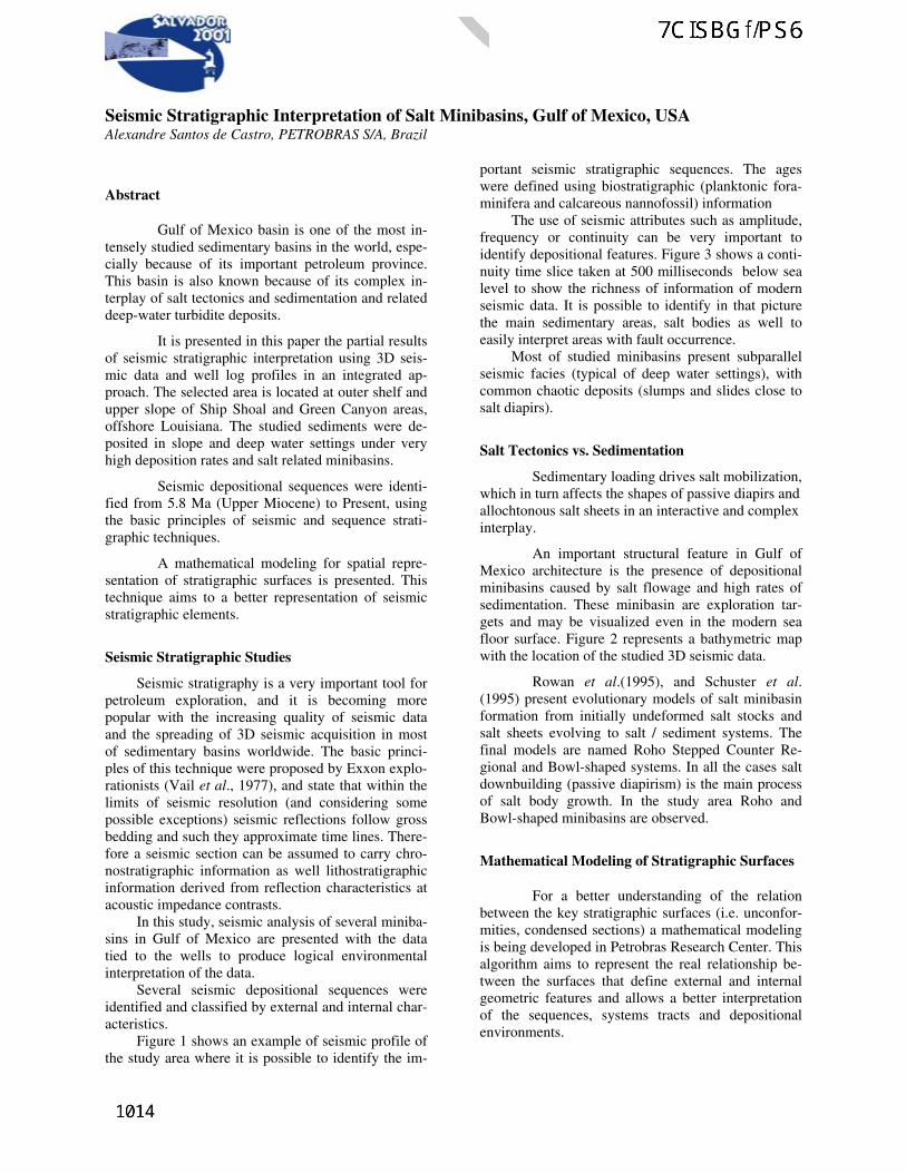
Seismic Stratigraphic Interpretation of Salt Minibasins, Gulf of Mexico, USAAlexandre Santos de Castro, PETROBRAS S/A, Brazil

Abstract

Gulf of Mexico basin is one of the most in-tensely studied sedimentary basins in the world, espe-cially because of its important petroleum province.This basin is also known because of its complex in-terplay of salt tectonics and sedimentation and relateddeep-water turbidite deposits.

It is presented in this paper the partial resultsof seismic stratigraphic interpretation using 3D seis-mic data and well log profiles in an integrated ap-proach. The selected area is located at outer shelf andupper slope of Ship Shoal and Green Canyon areas,offshore Louisiana. The studied sediments were de-posited in slope and deep water settings under veryhigh deposition rates and salt related minibasins.

Seismic depositional sequences were identi-fied from 5.8 Ma (Upper Miocene) to Present, usingthe basic principles of seismic and sequence strati-graphic techniques.

A mathematical modeling for spatial repre-sentation of stratigraphic surfaces is presented. Thistechnique aims to a better representation of seismicstratigraphic elements.

Seismic Stratigraphic Studies

Seismic stratigraphy is a very important tool forpetroleum exploration, and it is becoming morepopular with the increasing quality of seismic dataand the spreading of 3D seismic acquisition in mostof sedimentary basins worldwide. The basic princi-ples of this technique were proposed by Exxon explo-rationists (Vail et al., 1977), and state that within thelimits of seismic resolution (and considering somepossible exceptions) seismic reflections follow grossbedding and such they approximate time lines. There-fore a seismic section can be assumed to carry chro-nostratigraphic information as well lithostratigraphicinformation derived from reflection characteristics atacoustic impedance contrasts.

In this study, seismic analysis of several miniba-sins in Gulf of Mexico are presented with the datatied to the wells to produce logical environmentalinterpretation of the data.

Several seismic depositional sequences wereidentified and classified by external and internal char-acteristics.

Figure 1 shows an example of seismic profile ofthe study area where it is possible to identify the im-

portant seismic stratigraphic sequences. The ageswere defined using biostratigraphic (planktonic fora-minifera and calcareous nannofossil) information

The use of seismic attributes such as amplitude,frequency or continuity can be very important toidentify depositional features. Figure 3 shows a conti-nuity time slice taken at 500 milliseconds below sealevel to show the richness of information of modernseismic data. It is possible to identify in that picturethe main sedimentary areas, salt bodies as well toeasily interpret areas with fault occurrence.

Most of studied minibasins present subparallelseismic facies (typical of deep water settings), withcommon chaotic deposits (slumps and slides close tosalt diapirs).

Salt Tectonics vs. Sedimentation

Sedimentary loading drives salt mobilization,which in turn affects the shapes of passive diapirs andallochtonous salt sheets in an interactive and complexinterplay.

An important structural feature in Gulf ofMexico architecture is the presence of depositionalminibasins caused by salt flowage and high rates ofsedimentation. These minibasin are exploration tar-gets and may be visualized even in the modern seafloor surface. Figure 2 represents a bathymetric mapwith the location of the studied 3D seismic data.

Rowan et al.(1995), and Schuster et al.(1995) present evolutionary models of salt minibasinformation from initially undeformed salt stocks andsalt sheets evolving to salt / sediment systems. Thefinal models are named Roho Stepped Counter Re-gional and Bowl-shaped systems. In all the cases saltdownbuilding (passive diapirism) is the main processof salt body growth. In the study area Roho andBowl-shaped minibasins are observed.

Mathematical Modeling of Stratigraphic Surfaces

For a better understanding of the relationbetween the key stratigraphic surfaces (i.e. unconfor-mities, condensed sections) a mathematical modelingis being developed in Petrobras Research Center. Thisalgorithm aims to represent the real relationship be-tween the surfaces that define external and internalgeometric features and allows a better interpretationof the sequences, systems tracts and depositionalenvironments.

Seismic Interpretation - Gulf of Mexico

Conclusions

It is reviewed in this work the fundamentalsof seismic stratigraphy and its applications of reser-voir exploration in areas of salt tectonics, and thedepositional geometries present in slope minibasins ofoffshore Gulf of Mexico.

The study was based on the integration of 3Dseismic data and well log profiles and biostratigraphy,and a detailed seismic facies analyses is presented.

Modern salt/sedimentation models are dis-cussed, with application in the study area.

References

Diegel, F.A., J.F. Karlo, D.C. Schuster, R.C. Shoupand P.R. Tauvers, 1995. Cenozoic structural evo-lution and tectono-stratigraphic framework of thenorthern Gulf Coast continental margin. In: M.P.AJackson. D.G.Robertson and S.Snelson, eds., SaltTectonics: a global perspective, AAPG Memoir65, p.109-151.

Rowan, M.G., 1995. Structural styles and evolution ofallochtonous salt, central Louisiana outer shelf andupper slope, In: M.P.A Jackson. D.G.Robertsonand S.Snelson, eds., Salt Tectonics: a global per-spective, AAPG Memoir 65, p.199-228

Rowan, M.G. and Weimer, P., 1998. Salt-sedimentinteraction, northern Green Canyon and EwingBank (offshore Louisiana), northern Gulf of Mex-ico. AAPG Bull., V.82, No.5B, p 1055-1082.

Schuster, D.C., 1995. Deformation of allochtonoussalt structural systems, Eastern Louisiana GulfCoast. In: M.P.A Jackson. D.G.Robertson andS.Snelson, eds., Salt Tectonics: a global perspec-tive, AAPG Memoir 65, p.177-198.

Vail, P.R., Mitchum, R.M.Jr., Todd, R.G., Widmier,J.M., Thompson,.S.III,Sangree, J.B. Bubb, J.N.and Hatfeild, W.G., 1977. Seismic stratigraphy andglobal changes in sea level. In: Seismic stratigra-phy – Applications to hydrocarbon exploration.C.E. Payton (ed.), AAPG Memoir 26, p.49-62.

Acknowledgments

The author would like to acknowledge Petro-bras, University of Colorado at Boulder and Uni-versidade Federal do Rio de Janeiro(UFRJ/COPPE) for allowing the opportunity ofthis doctorate research.

Seismic Interpretation - Gulf of Mexico

Figure 1 – Northeast–southwest seismic profile showing the interpreted seismic depositional sequences of abowl-shaped minibasin. The actual configuration of salt diapirs are not clear in this image.

Figure 2 – Bathymetric map of Gulf of Mexico basin with the location of study area (from Diegelet al, 1995). It is possible to notice the existence of the salt-driven minibasins at the sea floor surface allover the continental slope.

Seismic Interpretation - Gulf of Mexico

Figure 3 – Seismic time-slice of continuity data of the study area taken at 560 milliseconds. Lighterareas represent depositional minibasins and darker areas are salt bodies. Faults related to salt tectonics arealso easier to identify in this kind of display.

Tectonics and Stratigraphy of East Java Sea North of Madura Island, IndonesiaWisley de Oliveira Martins and Roberto Fainstein Schlumberger, Rio de Janeiro

Abstract

The purpose of this paper is to provide a modernregional geological and geophysical interpretation ofthe East Java Sea Basin. The basis for this seismicinterpretation are 798 kilometers of recently acquirednon-exclusive 2D seismic data and ties to well data.

The East Java Sea displays excellent examplesof Miocene to present-day structural inversion of aback-arc Paleogene basin system. The structuralgeometry of these inversions has been analysed by aseries of non-exclusive seismic surveys thatdemonstrate significant lateral variation in structuralstyle.

Driving mechanisms of structural inversion havebeen assessed by modelling motions of the Eurasian,Indian Ocean, Australian and Pacific plates during theNeogene. The evolution of such inversion within theEast Java Sea is interpreted as a function of thecollision of the Australian Plate with the Sunda Arc.Moreover, the relative convergence rate and directionof the subducting Indian Ocean Plate and the S.E.Eurasian Plate affect inversion.

Two tectonic phases have been identified, onecontrolling the Paleogene rift and the othercontrolling the Neogene faulting

Structures formed during the Late Miocene wereidentified in seismic data. They represent prospectiveexploration features. On the shelf areas, patch reefsand shallow marine sandstone ranging from Oligo-cene to Middle Miocene are the targets for explora-tion. Reef limestones from the Pliocene age wheresealed by Recent mudstones are also of interest.

Introduction – Non-Exclusive Survey

The East Java Sea Basin is part of back-arc ba-sins that developed peripheral to the Sunda Shield,these extend from North Sumatra to Central Sulawesi.Onshore East Java is well explored and has beenproducing oil since the late 19th century. Explorationof the East Java Sea began in the early 1970´s and is asignificant gas province. It is also have to currentlysub-economic oil and gas finds.

Non-Exclusive Seismic Surveys have been con-ducted by Schlumberger WesternGeco since 1993 inall of the Souteast Asia Offshore Basins (Figure 1)with the aim of improving the petroleum geologyknowledge of this area.

Modern data are now available on most of theoffshore Tertiary Basins such as Palawan Basin off-shore Philippines, Natuna Sea off Indonesia, Anda-man Sea offshore Myanmar and North Sumatra, off

Madura Island (Figure 2) and off North Bali in theEast Java Sea Basin and in the MahakamDelta/Makasar Strait region. In the Pre-Terciary Ba-sins of the Eastern Indonesia and northwest shelf ofAustralia modern deep-water seismic data were alsoacquired and interpreted.

Figure 1: Location of non-exclusive 2D surveys un-dertaken in the Southeast Asia Archipelago by Wes t-ernGeco.

Figure 2: Location Map – Offshore North MaduraIsland Non-Exclusive Seismic Survey, East Java Sea.

Tectonic Setting

The sub-basins of East Java Sea are part of anextensive, complex, basin system that has developedaround the margins of the SE EurasianPlate (Figure3). The orientation of major fault zones defining thesesub-basins boundaries varies around this margin.Three distinct trends are recognised. In the area of theMakassar Basin the main fault systems are orientatedapproximately NE-SW, parellel to the coastlines ofEast Kalimantan and West Sulawesi which form theflanks of the basin. Faults of this orientation continueSW into the East Java Sea where they define sub-basins such as the Masalima Trough, Central Deepand Muriah Trough. NW-SE trending faults are pres-ent within the Makassar Basin, notably north of the

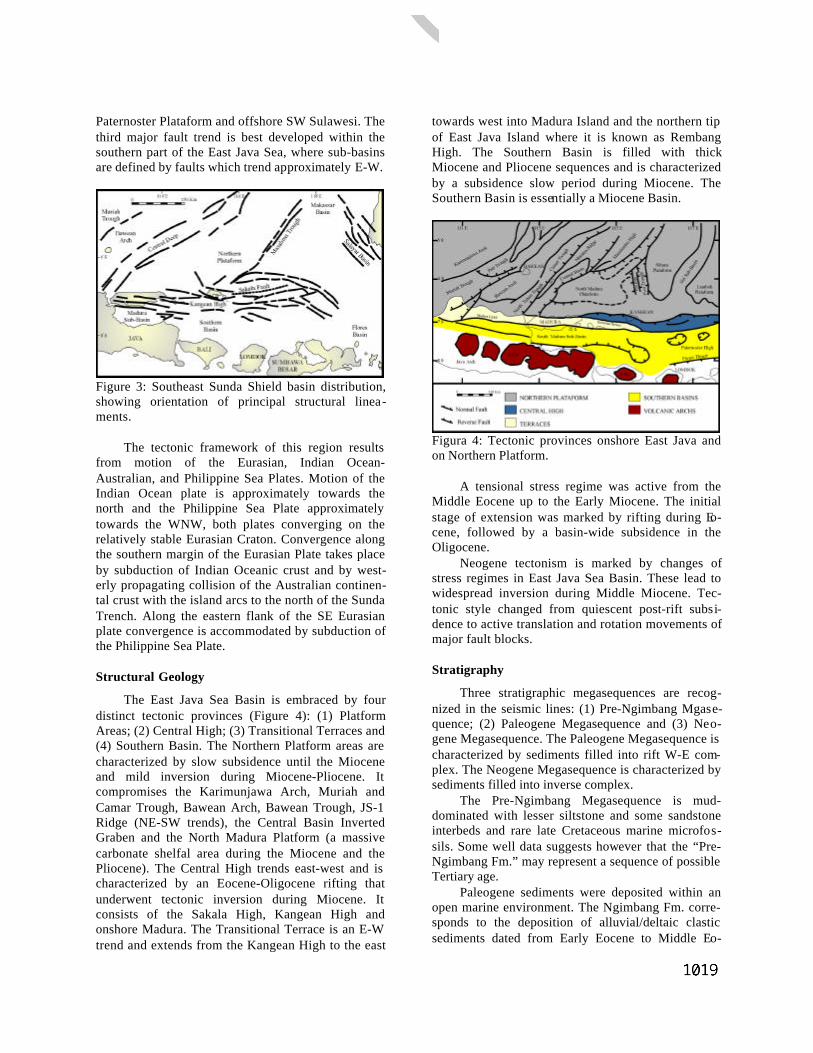
Paternoster Plataform and offshore SW Sulawesi. Thethird major fault trend is best developed within thesouthern part of the East Java Sea, where sub-basinsare defined by faults which trend approximately E-W.

Figure 3: Southeast Sunda Shield basin distribution,showing orientation of principal structural linea-ments.

The tectonic framework of this region resultsfrom motion of the Eurasian, Indian Ocean-Australian, and Philippine Sea Plates. Motion of theIndian Ocean plate is approximately towards thenorth and the Philippine Sea Plate approximatelytowards the WNW, both plates converging on therelatively stable Eurasian Craton. Convergence alongthe southern margin of the Eurasian Plate takes placeby subduction of Indian Oceanic crust and by west-erly propagating collision of the Australian continen-tal crust with the island arcs to the north of the SundaTrench. Along the eastern flank of the SE Eurasianplate convergence is accommodated by subduction ofthe Philippine Sea Plate.

Structural Geology

The East Java Sea Basin is embraced by fourdistinct tectonic provinces (Figure 4): (1) PlatformAreas; (2) Central High; (3) Transitional Terraces and(4) Southern Basin. The Northern Platform areas arecharacterized by slow subsidence until the Mioceneand mild inversion during Miocene-Pliocene. Itcompromises the Karimunjawa Arch, Muriah andCamar Trough, Bawean Arch, Bawean Trough, JS-1Ridge (NE-SW trends), the Central Basin InvertedGraben and the North Madura Platform (a massivecarbonate shelfal area during the Miocene and thePliocene). The Central High trends east-west and ischaracterized by an Eocene-Oligocene rifting thatunderwent tectonic inversion during Miocene. Itconsists of the Sakala High, Kangean High andonshore Madura. The Transitional Terrace is an E-Wtrend and extends from the Kangean High to the east

towards west into Madura Island and the northern tipof East Java Island where it is known as RembangHigh. The Southern Basin is filled with thickMiocene and Pliocene sequences and is characterizedby a subsidence slow period during Miocene. TheSouthern Basin is essentially a Miocene Basin.

Figura 4: Tectonic provinces onshore East Java andon Northern Platform.

A tensional stress regime was active from theMiddle Eocene up to the Early Miocene. The initialstage of extension was marked by rifting during Eo-cene, followed by a basin-wide subsidence in theOligocene.

Neogene tectonism is marked by changes ofstress regimes in East Java Sea Basin. These lead towidespread inversion during Middle Miocene. Tec-tonic style changed from quiescent post-rift subsi-dence to active translation and rotation movements ofmajor fault blocks.

Stratigraphy

Three stratigraphic megasequences are recog-nized in the seismic lines: (1) Pre-Ngimbang Mgase-quence; (2) Paleogene Megasequence and (3) Neo-gene Megasequence. The Paleogene Megasequence ischaracterized by sediments filled into rift W-E com-plex. The Neogene Megasequence is characterized bysediments filled into inverse complex.

The Pre-Ngimbang Megasequence is mud-dominated with lesser siltstone and some sandstoneinterbeds and rare late Cretaceous marine microfos-sils. Some well data suggests however that the “Pre-Ngimbang Fm.” may represent a sequence of possibleTertiary age.

Paleogene sediments were deposited within anopen marine environment. The Ngimbang Fm. corre-sponds to the deposition of alluvial/deltaic clasticsediments dated from Early Eocene to Middle Eo-

cene. During Middle Eocene, a wide area was stillemergent which provided good source for clasticsdeposition. The Late Eocene corresponds to the depo-sition of marine shales and marine carbonate, withpossible reef development over previous basementhighs on the edges of grabens. Eocene Ngimbangshales are source rocks yielding hydrocarbon ocur-rences.

As transgression continued troughout Early Oli-gocene time, the relief of land masses was greatlyreduced. Reef development continued in some areas,although regionally these carbonate sequences gradu-ally become more marly platform deposition. TheseLate Eocene-Early Oligocene sediments are known asthe CD Formation.

During Late Early Oligocene time, the northernpart of the Java Sea was uplifted concurrently with aworldwide eustatic sea level fall and the area wasflooded by the marine clastics of the Kujung Unit III.In some restricted areas, shallow water limestonescontinued to be deposited throughout this regressiveperiod. Shales of the Kujung III are within the oilwindow in many instances.

During Late Oligocene time the area again un-derwent a transgressive event. Kujung unit II clasticsand shalow water limestones were deposited at thistime. The Kujung II carbonates are oil and gas reser-voirs accumulations northwest of Madura. DuringLate Oligocene and Early Miocene time, massivelimestones of the Kujung Unit I (gas reservoir) devel-oped reefs in areas favourable for their growth.

The Neogene Megasequence during Early Mio-cene time uplift in Kalimantan led to an influx of fineclastics of the OK Formation. These overlies theKujung I and provides regional seal. This influx ofclastics terminated the Kujung reef growth, except ina few areas (e.g. Rancak Limestone). Transgressiveshallow marine deposition resumed during late Mid-dle Miocene through Pliocene time, where it is re-corded by fine clastics and carbonates of the KarrenFm. Pliocene and Recent clays complete the overbur-den (Figure 5).

Seismic Interpretation

Eight seismic horizons representative of struc-turing were interpreted: (1) Basement; (2) Pre-Ngimbang Fm; (3) Ngimbang Fm; (4) Kujung III Fm;(5) Kujung II Fm; (6) Kujung I Fm; (7) OK Fm and(8) Early Pliocene.

Basement consists essentially of NE-SW trend-ing platform area further north, and an inverted half-graben known as Central Depression towards south.Near the Madura coastline the central trough is bor-dered by another basement high (Figure 6).

Figure 5: Generalized Stratigraphy of East Java andcorrespondent tectonic episodes.

Figure 6: Basament Map.

The main area of inversion trends along a NE-SW direction. All the tectonic provinces of East Javaare recognised in the 2D seismic lines. Paleohigh andpaleolow structures are distinguished by lithologicalthinning and thickening over the older Eocene units.Seismic interpretration also revealed the platformareas unaffected by tectonic inversion and the local-ized half-grabens which were subsequently inverted(Figure 7 and 8).

The Kujung I Fm. marks the seismic boundarybetween the Paleogene extension and the Neogeneinversion. Early Miocene and younger uplifts haveaffected a large area of the East Java Sea. These up-lifts have evolved by reversal movement on normalfaults which had previously accomodated Paleogenesubsidence. The grabens and half-grabens whichexisted until early Miocene were inverted and thelargest anticlines were generated (Figure 7 and 8).

Three distinct Neogene units are recognized inseismic lines: 1) Early to mid Miocene highstandprogradation; 2) Transgressive Late Miocene termi-

nated by Early Pliocene lowstand and 3) Plio-Pleistocene sedimentation.

Figure 7: Seismic record gpmi96-103.

Figure 8: Seismic record gpmi96-104.

Conclusions

The East Java Sea Basin have all tectonic re-queriments for hydrocarbon entrapment: source rockkitchens; development of good reservoir and sealfacies; and a clear structural distinction between earlybasement highs and inverted graben structures.

Paleogene tensional stresses led to the develop-ment of NE-SW trending tilted horst blocks and gra-bens. Neogene tectonism related to strike-slip move-ment led to development of inversion structures andis the major structural control in the region.

The newly acquired non-exclusive seismic sur-vey enabled imaging of deeper beds beneath the car-bonates. Seismic interpretation unraveled new ex-ploratory plays: 1) Broad young anticlines of thezones of inversion are attractive Kujung I and II tar-gets (Figure 9); 2) Deeper Eocene Ngimbang playsare yet to be drilled. These consist of structural clo-sures and of stratigraphic wedges onlapping base-ment.

Figure 9: Structural map of Kujung Fm. Carbonates.Several Kujung I and Kujung II prospects areattractive.

References

Ardhana, W. 1993. A Depositional Model For TheEarly Middle Miocene Ngrayong Formation andImplications For Exploration In The East JavaBasin. Proceedings Of The IndonesianPetroleum Association, 22nd Annual Convention:395-443.

Beddoes, L. R. 1981. Hydrocarbon Plays In TertiaryBasins Of Southeast Asia. Energy, 6 (11): 1141-1163.

Bransden, P. J. E. & Mattews, S. J. 1992. StructuralAnd Stratigraphic Evolution Of The East JavaSea, Indonesia. Proceedings Of The IndonesianPetroleum Association, 21st Annual Convention:417-453.

Fainstein, R. 1997. Seismic Interpretation OffshoreMadura, East Java Sea, Society ExplorationGeophysicists, Annual International Meeting,Dallas.

Fainstein, R. & Raharja, M. 1989. PagerunganSeismic Interpretation. Atlantic Richfield BaliNorth Publication, 1 (text), 2 (maps) and 3(seismics).

Hamilton, W. 1979. Tectonics Of The IndonesianRegion. US Geological Survey ProfessionalPaper, 1078.

Acknowledgments

We would like to thank Schlumberger West-ernGeco for permission to publish this work andSchlumberger GeoQuest for the seismic interpretationsoftwares.

Volume Interpretation TechniquesMárcio Spínola, Landmark Graphics, BrasilCarlos Eduardo Abreu, PETROBRAS S/A Brasil

Abstract

Digital Volumetric Images play important role inmedical imaging as well in geology and geophysics.In the past recent 6 years advances in computer hard-ware and software have brought this technology thatbegan to be applied for medical purposes and now iswidely available for geoscientists.

This work attempts to discuss volume interpretationtechniques of 3D seismic data. The techniques arepresented with emphasis on definitions and function-ality. Fist we present the volume visualization andinterpretation techniques, including color maps, his-tograms, opacity, attribute analysis, horizon, faultsand Voxbody1 interpretation. Further we presentAdvanced Volume Interpretation techniques1, in-cluding image processing covering automated volumerecognition (Body Labeling), morphology operations(Morphology), and copy of seismic data using pre-defined masks (Shape Cutter). Together all thesetools can be combined to create structural or strati-graphic interpretation workflows. Insights using realdata as examples are given.

1. Introduction

Digital Volumetric Images are 3D image arrays cor-responding to a stack of two-dimensional slices pro-duced by some scanning technology (Lohmann,1998). Volumetric images can be generated frommany different methods, for instance in computertomography (based on X-ray beans), magnetic reso-nance tomography, ultrasound, microscopy, andseismic acquisition and processing. Such images playimportant role in medical imaging as well as inter-pretation of geological bodies from 3D seismic vol-ume.

3D seismic volumes are time or depth sequences of2D images obtained from seismic acquisition andprocessing. The building blocks of three-dimensionalimages are volume elements or voxels2. A voxel, orvolume pixel, is the smallest distinguishable box-shaped part of a three-dimensional image. Voxels areused to render seismic attributes like amplitude,

1Some definitions follow the Landmark’s volumevisualization and interpretation tool EarthCube2 http://www.pcwebopedia.com/TERM/v/voxel.html

acoustic impedance, coherence, etc. For a true 3Dimage, voxels must undergo opacity transformation.Opacity transformation gives voxels different opacityvalues. This is important when it is crucial to exposeinterior details of an image that would otherwise behidden by darker more opaque outside-layer voxels.This work attempts to discuss volume visualizationand interpretation techniques of 3D seismic data. Firstwe discuss some of most the frequent visualizationand volume interpretation techniques including colormaps, histograms, opacity, attribute analysis, horizon,faults and Voxbody2 interpretation. Further we presentAdvanced Volume Interpretation techniques, includ-ing image processing derived from medical industry.

2. 3D Visualization Techniques

2.1. Working with synthetics (Tie well to seismic)

One of the essential jobs in volume interpretation is totie available well information to seismic. This proce-dure allows geoscientists to make correlation betweenformation tops interpreted from well logs to the ob-served seismic, being critical to the quality of inter-pretation.Henry (1997) pointed out that without the under-standing of wavelet as the filter through which geol-ogy is viewed when interpreting image provided byseismic data, there are many equally valid geologicalinterpretations of the actual subsurface geologyThe benefits about identify high frequency well in-formation (lithology, markers) on low frequencyseismic information (high area coverage) is to provideinterpreter key links to identify reservoir facies. Alsoto it is part of workflow to generate time depth tablesthat can be used to display well logs in time, build 3Dvelocity models for posterior conversion of seismictraces from time to depth.

2.2. Color maps and histograms

Once seismic volume is loaded from disk to the com-puter RAM memory for visualization purposes, inter-preters can highlight events on seismic data by simplyaddressing a color table to a range of attribute values.The objective is to emphasize seismic features thatreflect changes in the acoustic property of the rocks(impedance) and may be closely related to lithologychanges, facies variation, presence of fluid or gassaturation. Doing so the contrast and visibility of suchfeatures are increased.

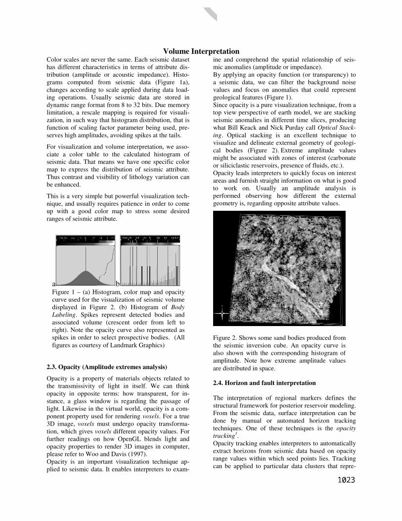
Volume Interpretation

a bFigure 1 – (a) Histogram, color map and opacitycurve used for the visualization of seismic volumedisplayed in Figure 2. (b) Histogram of BodyLabeling. Spikes represent detected bodies andassociated volume (crescent order from left toright). Note the opacity curve also represented asspikes in order to select prospective bodies. (Allfigures as courtesy of Landmark Graphics)

Figure 2. Shows some sand bodies produced fromthe seismic inversion cube. An opacity curve isalso shown with the corresponding histogram ofamplitude. Note how extreme amplitude valuesare distributed in space.

Color scales are never the same. Each seismic datasethas different characteristics in terms of attribute dis-tribution (amplitude or acoustic impedance). Histo-grams computed from seismic data (Figure 1a),changes according to scale applied during data load-ing operations. Usually seismic data are stored indynamic range format from 8 to 32 bits. Due memorylimitation, a rescale mapping is required for visuali-zation, in such way that histogram distribution, that isfunction of scaling factor parameter being used, pre-serves high amplitudes, avoiding spikes at the tails.

For visualization and volume interpretation, we asso-ciate a color table to the calculated histogram ofseismic data. That means we have one specific colormap to express the distribution of seismic attribute.Thus contrast and visibility of lithology variation canbe enhanced.

This is a very simple but powerful visualization tech-nique, and usually requires patience in order to comeup with a good color map to stress some desiredranges of seismic attribute.

2.3. Opacity (Amplitude extremes analysis)

Opacity is a property of materials objects related tothe transmissivity of light in itself. We can thinkopacity in opposite terms: how transparent, for in-stance, a glass window is regarding the passage oflight. Likewise in the virtual world, opacity is a com-ponent property used for rendering voxels. For a true3D image, voxels must undergo opacity transforma-tion, which gives voxels different opacity values. Forfurther readings on how OpenGL blends light andopacity properties to render 3D images in computer,please refer to Woo and Davis (1997).Opacity is an important visualization technique ap-plied to seismic data. It enables interpreters to exam-

ine and comprehend the spatial relationship of seis-mic anomalies (amplitude or impedance).By applying an opacity function (or transparency) toa seismic data, we can filter the background noisevalues and focus on anomalies that could representgeological features (Figure 1).Since opacity is a pure visualization technique, from atop view perspective of earth model, we are stackingseismic anomalies in different time slices, producingwhat Bill Keack and Nick Purday call Optical Stack-ing. Optical stacking is an excellent technique tovisualize and delineate external geometry of geologi-cal bodies (Figure 2). Extreme amplitude valuesmight be associated with zones of interest (carbonateor siliciclastic reservoirs, presence of fluids, etc.).Opacity leads interpreters to quickly focus on interestareas and furnish straight information on what is goodto work on. Usually an amplitude analysis isperformed observing how different the externalgeometry is, regarding opposite attribute values.

2.4. Horizon and fault interpretation

The interpretation of regional markers defines thestructural framework for posterior reservoir modeling.From the seismic data, surface interpretation can bedone by manual or automated horizon trackingtechniques. One of these techniques is the opacitytracking1.Opacity tracking enables interpreters to automaticallyextract horizons from seismic data based on opacityrange values within which seed points lies. Trackingcan be applied to particular data clusters that repre-

Volume Interpretationsent extreme continuous coherent reflectors and might(or not) be associated to the reservoir.

Although some problems may occur when no con-tinuous or coherent reflectors associated for instancewith erosional unconformities or salt structures arepresent, generally some regional markers with highimpedance contrast can produce extensive horizonpicking. They may represent sequence boundaries, forinstance, maximum flooding surfaces (MSF). In suchcases opacity tracking furnishes enormous advantageover the traditional interpretative workflow done lineby line and trace by trace. Even more complex casescan be worked on dividing large areas into small onesand performing a re-tracking when necessary. Hereinterpreter acts more like a supervisor, worried aboutQC of the automated interpretation.

Regarding Fault interpretation, Seismic plane anima-tion is a suitable visualization technique to detect andidentify faulted zones and how it evolves throughvolume, appearing or disappearing in differentline/traces. Also it is a good method to detect thepresence of individual subtle faults.

Fault interpretation task is better accomplished bymeans of using seismic attributes like coherence cube.When mapped on horizon slices, coherence cubeinformation can provide good insights to correctlyposition faults. Also coherence volumes can be visu-alized and interpreted on time slices, seismic planesor horizon slices.

2.5. Attribute analysis

Seismic attributes can be calculated in a time windowaround interpreted horizon. The result is a map thatthat can summarize aspects of seismic data within astratigraphic sequence.

These maps displayed in 3D as overlays on a givenhorizon, stresses structure and can be combined withdifferent types of information on its real spatial loca-tion. It helps interpreter to identify potential areaswhere better net to gross, gross porosity, presence ofchannels, lobes, faults, tunning effects are located,acting as guiders for prospect delineation and wellpath planning.

There is no rule in order to select a particular attrib-ute. It depends on the prospect and the particularinterest in study. Some frequent attributes are: RMSamplitude, instantaneous phase, half time energy,total energy, maximum amplitude, etc.

Instantaneous phase can enhance weak coherenceevents that may be helpful to identify pinchouts, in-

ternal depositional geometries, faults pinchouts, oiland gas contact changes, etc (Landmark, 1999). Thecalculated root mean square attribute (RMS) is sensi-tive to extreme amplitude values.

2.6. Voxbody and Volumetrics

Once reservoir targets where identified in particularzones, one can isolate different geologic intervals andcompute volumetrics through Voxbody Interpreta-tion1. Voxbody consists of a set of connected voxels,and can be generated by tracking or sculpting seismicvolume.Tracking consists in selecting parameters like ampli-tude range, neighborhood criteria and picking a validseed point (or multiple seed points) from the 3Dseismic. Sculpting consists in defining an upper andlower surface (actually could be the same surfaceshifted in time/depth) and removing the seismic dataabove and below the bounding intervals. The result isa slab of seismic data that can contain for instance aparasequence.Formation isolation via sculpting consists in a valu-able technique when combined with other visualiza-tion techniques like opacity. An optical stacking fur-nishes much information about geometry and stratig-raphy.

3. Advanced Volume Interpretation

Advanced volume interpretation tool include image-processing techniques (from Foster Findley Associ-ates) allowing voxel manipulation, automated featurerecognition (Body Labeling), morphology operations(Morphology), seismic volume math (useful for 4Dseismic) and copy of seismic data using pre-definedmasks (Shape Cutter). Together all these tools can becombined to create structural or stratigraphic inter-pretation workflows.These tools enhance structural or stratigraphic inter-pretation workflows, enabling manipulation of multi-ple seismic attributes that combined with other typesof information can be user to infer lithology, stratig-raphy and other properties.

3.1. Automated feature recognition (body labeling)

Body labeling1 allows interpreters to automated ex-tract geological features without seed picking. It con-sists in defining volumetric criteria for isolating 3Dfeatures.Four parameters are taken into account by the algo-rithm for accepting or rejecting geological bodies:amplitude range, minimum and maximum number ofvoxels and connectivity. The output produces a set of

Volume Interpretation

Figure 7. Captured seismic ampli tudes of isolatedreservoir bodies. Note the presence of channels andassociated crevasse splays facies.

Figure 6. Masks produced by body labeling algo-rithm. Only prospective bodies are shown.

bodies sorted according to volume size. Each bodycontains information about seismic continuity.Figure 6 shows the results of body labeling run in thesame volume as Figure 2. Note that it produces amuch clear image. Each detected body produces aspike and an opacity curve can be applied to isolatepossible sand bodies (Figure 5). Each continuousindividual body receives a label and an associatedcolor (that explains the word labeling). Volumetricsthen can straight be calculated.

3.2. Shape cutter

Next step after isolating reservoir bodies would bepopulating these regions with seismic data (Figure 7).One of the benefits of isolating seismic is workingwith seismic attributes of the interest zones, forvolumetrics computation, horizon interpretation(voxbody wrapping) or body labeling. Later we aregoing to use this information to guide us in the defi-nition of the planned well targets.

3.3. Morphology

Morphology is frequently used after sub-volumedetection. Processing algorithms like Opening orclosing can be applied in order to fill out holes orextend volumes beyond detected regions. Furtherreading about morphology operations can be found inStoyan at all (1995{ 1985} ).

4. Conclusions

We review a set volume visualization and interpreta-tion techniques. All these tools can be used in struc-tural and stratigraphic interpretation workflows to

enhance prospect evaluation and characterization. Weview volumetric interpretation and visualization as anew form of communication. Also new developmentsin the hardware and software from universities andindustry will greatly impact the reservoir modelli ngworkflow. New virtual reali ty (VR) application de-velopments will bring new perspectives for the recentfuture, and the use of gloves for hand picking (insteadof mouse picking) and voice recognition are some ofthe innovative approaches expected for the next years.

References

Keach B, & Purday, N. 2000, Immersive TrainingClass. September 18-23. Houston – EUA.

Henry S., 2000, Pitfalls in Synthetics. The LeadingEdge, June, 604-606.

Lohmann, G., 1998, Volumetric Image Analysis:Wiley & Teubner, 243p.

Landmark, OpenBooks. Postack Family ReferenceManual. Marck 1999. Landmark Graphics Corp.

Stoyan, D., Kendall , W. S., Mecke, J.. StochasticGeometry and its Applications. West Sussex,England: Wiley, 1995{ 1985} . 436p.

Woo M., Neider, J., Davis T., 1997. OpenGL Pro-gramming Guide. Addison-Wesley DevelopersPress. 2nd Ed. Massachusetts. 650p.

Acknowledgments

We would like to thank PETROBRAS and LAND-MARK GRAPHICS for the courtesy to publish thiswork. We are also grateful to the professionals, NickPurday, Bill Keach and Yerko Guerra for the usefullessons on volume interpretation.