21st International Conference on Parallel Computational Fluid Dynamics – Moffett Field, CA – May 2009

Accelerating Clean Coal Gasifier Designswith Hybrid MPI/OpenMP High Performance Computing

A. Gel, S. Pannala, R. SankaranC. Guenther, M. Syamlal, T. O’Brien

=0.3 m

H=1

5.3

m .

Spiral

2

Team Members

•Aytekin Gel, ALPEMI Consulting, LLC •Chris Guenther, National EnergyTechnologyLaboratory•Madhava Syamlal, National EnergyTechnologyLaboratory•Thomas O’Brien, National EnergyTechnologyLaboratory•Ramanan Sankaran Oak Ridge National Laboratory (ORNL)•Sreekanth Pannala Oak Ridge National Laboratory (ORNL)and• Industrial Partners

3

Outline

• Motivation for Simulation Based Gasifier Design

• MFIX code• Performance Improvements for

MFIX• Preliminary results on hybrid

mode operation of MFIX on Cray XT5 and XT4 at NCCS

• Conclusions

4

Can we use the world’s most abundant and widely distributed fossil fuel source in a

different way?

An artist’s rendition depicts the goal of the FutureGen initiative, which aims to build the world’s first integrated sequestration and hydrogen production research power plant based on coal gasification.

Source: DOE Office of Fossil Energy

A coal-fired power plant in Conesville, Ohio

Source: Morgue File

Developing advanced coal technologies (as part of Clean Coal Initiative) to achieve zero emission of pollutants (e.g. CO2) while still remaining economically competitive

5

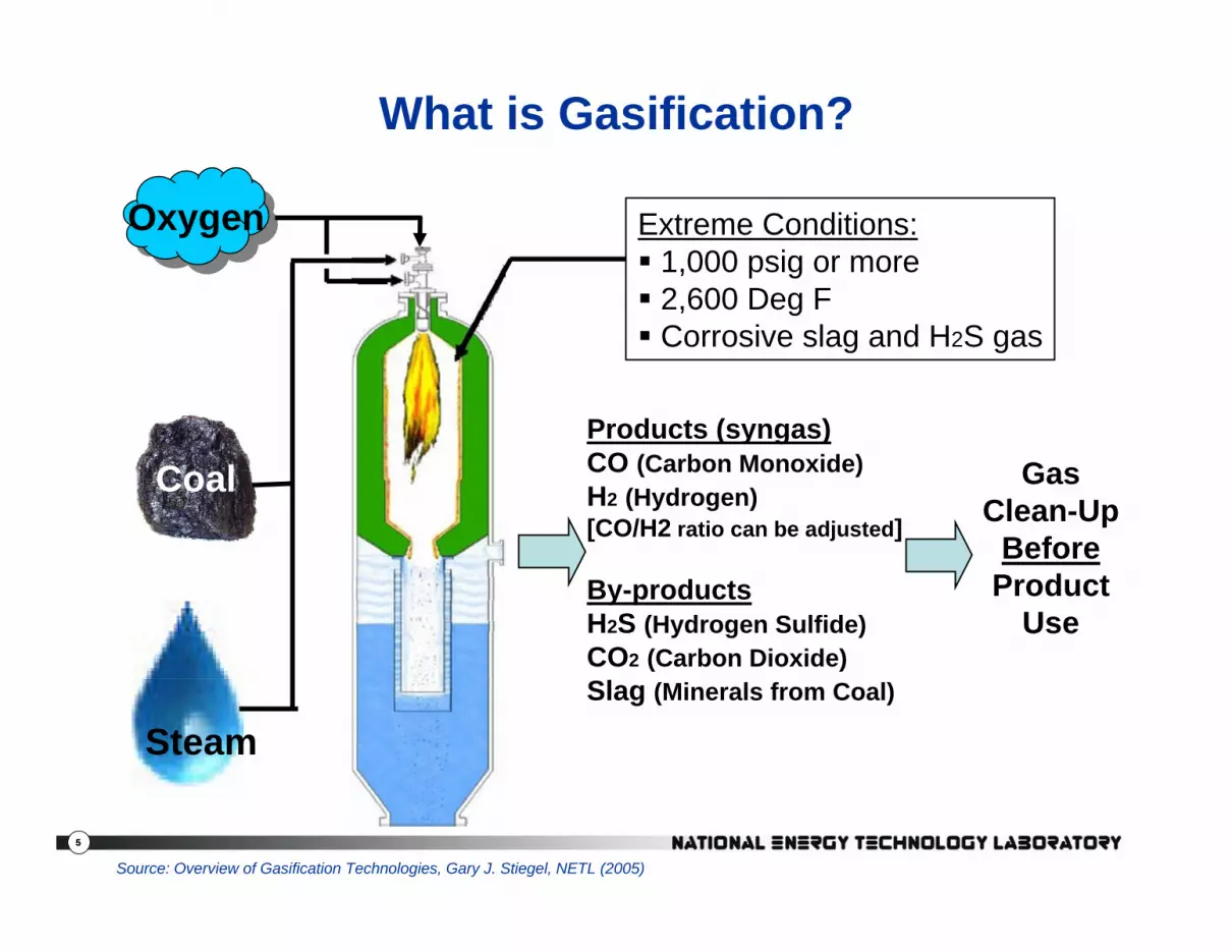
What is Gasification?

Coal

Steam

Oxygen Extreme Conditions: 1,000 psig or more 2,600 Deg F Corrosive slag and H2S gas

Products (syngas)CO (Carbon Monoxide)H2 (Hydrogen)[CO/H2 ratio can be adjusted]

By-productsH2S (Hydrogen Sulfide)CO2 (Carbon Dioxide)Slag (Minerals from Coal)

GasClean-Up

BeforeProduct

Use

Source: Overview of Gasification Technologies, Gary J. Stiegel, NETL (2005)

6

So what can you do with CO and H2 ?

Syngas

Transportation Fuels(Hydrogen)

Building Blocks forChemical Industry

CleanElectricity

Source: Overview of Gasification Technologies, Gary J. Stiegel, NETL (2005)

7

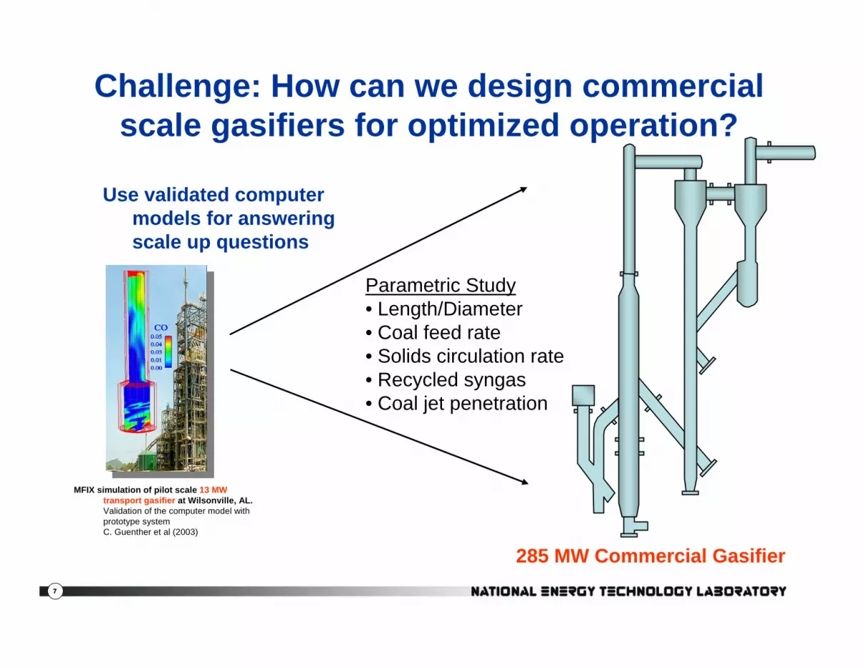
Challenge: How can we design commercial scale gasifiers for optimized operation?

285 MW Commercial Gasifier

Parametric Study• Length/Diameter• Coal feed rate• Solids circulation rate• Recycled syngas• Coal jet penetration

Use validated computer models for answering scale up questions

MFIX simulation of pilot scale 13 MW transport gasifier at Wilsonville, AL.Validation of the computer model with prototype system C. Guenther et al (2003)

8

Why Gasifier Simulations Are Computationally Intensive?

• Transient nature of gas-solid flows in industrial scale gasifier requires long computational times – Typical simulated time duration 10 to 15 sec

• Adaptive and small time-steps are required to resolve the physics, which is bounded by time-scales like particle relaxation time and collision time.– Average timestep ranging from 10-5 to 10-4 sec

• Strong non-linearity stems from the complex interactions between the gas and solid phases, the chemical species reactions, and heat transfer:– Several non-linear iterations required per timestep

9

Why Gasifier Simulations Are Computationally Intensive?

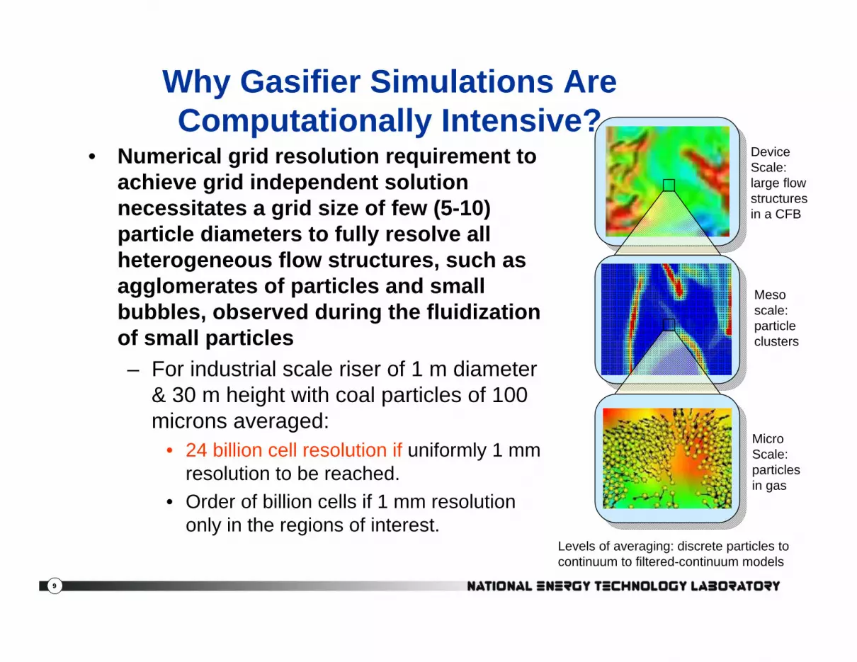
• Numerical grid resolution requirement to achieve grid independent solution necessitates a grid size of few (5-10) particle diameters to fully resolve all heterogeneous flow structures, such as agglomerates of particles and small bubbles, observed during the fluidization of small particles– For industrial scale riser of 1 m diameter

& 30 m height with coal particles of 100 microns averaged:

• 24 billion cell resolution if uniformly 1 mm resolution to be reached.

• Order of billion cells if 1 mm resolution only in the regions of interest.

Device Scale: large flow structures in a CFB

Mesoscale: particleclusters

Micro Scale: particles in gas

Levels of averaging: discrete particles to continuum to filtered-continuum models

10

• Multiphase computational fluid dynamics software that couples multi-phase hydrodynamics, heat transfer and chemical reactions

• Eulerian-Eulerian and Eulerian-Lagrangianapproach available.

• 3D Finite volume with Cartesian or cylindrical structured grid with recent addition of cut-cell

• Second order accurate in space and temporal discretization

• SMP (OpenMP), DMP (MPI) and Hybrid Parallel mode of execution options that runs on many HPC platforms including Linux clusters

• Open-source code and collaborative environment (http://www.mfix.org)

Tech-Transfer Award 2006

2007 R&D100 Award

11

Carbonaceous Chemistry for Continuum Modeling (C3M)

AshMoisture

Volatile Matter

Fixed Carbon

CaO

CaMg(CO3)2

MgO

CaCO3

coal sorbent

H2O CO + H2O CO2 + H2

CO2

1. Syamlal & Bissett 1992; 2. Wen et al. 1981 3. Peters 1979; 4. Westbrook & Dryer 1981

CO2 + H2O + CO

+ CH4 + H2 +Tar

[1]

O2

CO2

[2]

H2O H2 + CO

[2]

CO2

CO[2]

H2

CH4

[2]

CO2 + H2O + CO +

CH4 + H2 + Fixed Carbon

[1]

O2 [3,4]

CO2 + H2OO2

[3,4]

Excellence in Technology Transfer Award 2008

12

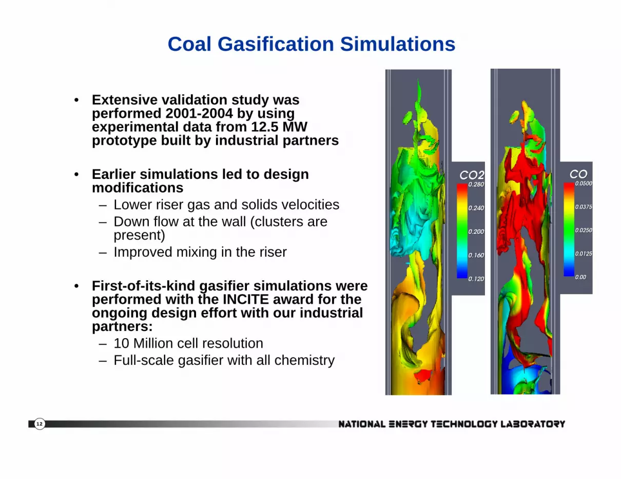
Coal Gasification Simulations

• Extensive validation study was performed 2001-2004 by using experimental data from 12.5 MW prototype built by industrial partners

• Earlier simulations led to design modifications– Lower riser gas and solids velocities– Down flow at the wall (clusters are

present)– Improved mixing in the riser

• First-of-its-kind gasifier simulations were performed with the INCITE award for the ongoing design effort with our industrial partners:– 10 Million cell resolution– Full-scale gasifier with all chemistry

13

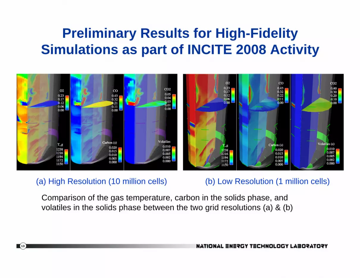
Preliminary Results for High-Fidelity Simulations as part of INCITE 2008 Activity

(a) High Resolution (10 million cells) (b) Low Resolution (1 million cells)

Comparison of the gas temperature, carbon in the solids phase, and volatiles in the solids phase between the two grid resolutions (a) & (b)

14

(a) High Resolution (10 million cells) (b) Low Resolution (1 million cells)

Comparison of the coal jet penetration between the two grid resolutions (a) and (b)

Preliminary Results for High-Fidelity Simulations as part of INCITE 2008 Activity

15

Performance Metric: Simulated time per wall-clock time

• Inherently transient nature of the process requires long duration of simulation before any useful insight can be gained – For 10M cell resolution, approximately 3M hrs on

jaguar(XT4)@NCCS used to generate 15 sec duration simulation in 2008.

• Target: Overnight turnaround (i.e., ~ 10 – 12 hrs)

16

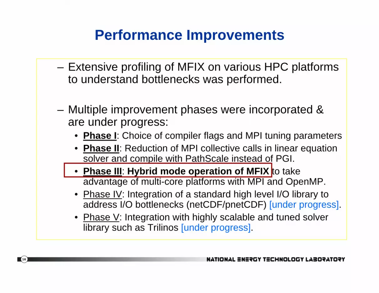
Performance Improvements

– Extensive profiling of MFIX on various HPC platforms to understand bottlenecks was performed.

– Multiple improvement phases were incorporated & are under progress:

• Phase I: Choice of compiler flags and MPI tuning parameters• Phase II: Reduction of MPI collective calls in linear equation

solver and compile with PathScale instead of PGI.• Phase III: Hybrid mode operation of MFIX to take

advantage of multi-core platforms with MPI and OpenMP.• Phase IV: Integration of a standard high level I/O library to

address I/O bottlenecks (netCDF/pnetCDF) [under progress].• Phase V: Integration with highly scalable and tuned solver

library such as Trilinos [under progress].

17

• Benchmarking problem with 10M cell grid resolution• Platform: Cray XT5@NCCS• MPI only and using all 8 cores on a node.• Time to solution measured for integrating over 100 steps of 2.5e-4 sec

– Initialization and I/O times are ignored and no replication of timings• Above 1032, more MPI ranks makes it slower for the current problem size

Preliminary Benchmarking Results on XT5 Execution Mode: MPI only and on 8 cores/node

18

Preliminary Benchmarking Results on XT5 Execution Mode: MPI only & using fewer cores/node

This is good, but can it get better if we put the remaining cores to use?

• As wall-clock time is valuable, used more nodes although not all cores were utilized.

• Having fewer MPI ranks per node gives solution faster

– Memory bandwidth limited portions of the code are sped

19

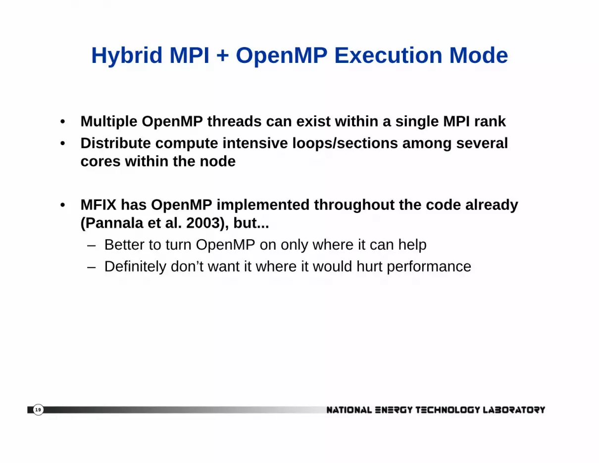
Hybrid MPI + OpenMP Execution Mode

• Multiple OpenMP threads can exist within a single MPI rank• Distribute compute intensive loops/sections among several

cores within the node

• MFIX has OpenMP implemented throughout the code already (Pannala et al. 2003), but...– Better to turn OpenMP on only where it can help– Definitely don’t want it where it would hurt performance

20

Where was the best MPI-only run spending time?

• Performance Profiling Tool: CrayPAT• Performance profiling of the 1032-rank MPI only job

gave the 25 % of time spent in two routines• leq_msolve and bc_phi have the most potential for

improvement through OpenMP threading

leq_msolvebc_phi

21

• First OpenMP enabled in the linear solver routines alone (leq_msolve).• And then also in the BC routine.• OpenMP brought the time down by 25% (457 sec to 335 sec)• But OpenMP in BC did not seem to help as much as the linear solver.

Why?

Preliminary Benchmarking Results on XT5 Execution Mode: MPI & OpenMP

22

Linear Solver vs. BC routine• A significant fraction of the time was spent in these two routines.

– ~16% in linear solver and ~8% in the BC– But, they were not doing the same thing

• The BC routine was dominated by memory access with very few compute operations

23

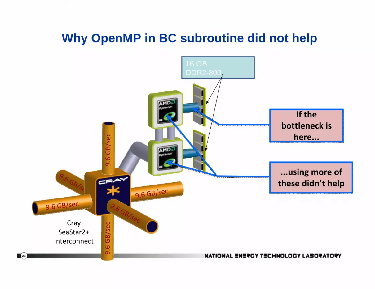
Why OpenMP in BC subroutine did not help

9.6 GB/sec

9.6  GB/s ec

9.6 GB/sec

9.6 GB/sec 9.6 GB/sec

9.6  GB/s ec

16 GB DDR2-800 memory

CraySeaStar2+

Interconnect

If the bottleneck is 

here...

If the bottleneck is 

here...

...using more of these didn’t help...using more of these didn’t help

24

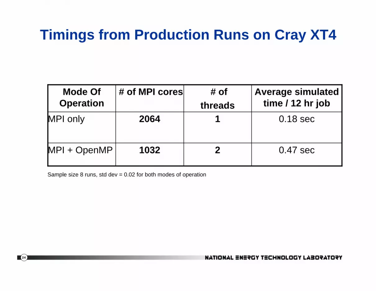
Timings from Production Runs on Cray XT4

0.47 sec21032MPI + OpenMP

0.18 sec12064MPI only

Average simulated time / 12 hr job

# of threads

# of MPI coresMode Of Operation

Sample size 8 runs, std dev = 0.02 for both modes of operation

25

Run Matrix Needed for Understanding Impact of Various Factors at Commercial Scale for a Given Gasifier Configuration

Estimated total HPC time resource requirement = 68 M hrs per gasifier configuration

26

Conclusions

• Parametric study using simulation based engineering is critical in understanding design factors and operational efficiencies for various configurations.

• Time-to-solution is key in the success of design and optimization of commercial scale gasifiers.

• Using hybrid MPI+OpenMP enabled a better performance to be achieved – better than attainable with MPI alone.

• MPI+OpenMP is not always best mode of execution, especially when memory bandwidth is the bottleneck

27

Questions?

AcknowledgmentsThe authors would like to acknowledge the support of the U.S. Department of Energy, Fossil Energy Advanced Research Program. The submitted manuscript has been authored by several contractors for the U.S. Government under Contract Numbers DE-AM26-04NT41817.670.01.03 and DE-AC05-00OR22725. This technical effort was performed in support of the National Energy Technology Laboratory's on-going research in multiphase flows under the RDS contract DE-AC26-04NT41817. Accordingly, the U.S. Government retains a non-exclusive, royalty-free license to publish or reproduce the published form of this contribution, or allow others to do so, for U.S. Government purposes. This research used resources of the National Center for Computational Sciences at Oak Ridge National Laboratory, which is supported by the Office of Science of the U.S. Department of Energy under Contract No. DE-AC05-00OR22725. Also this research used resources of the National Energy Research Scientific Computing Center, which is supported by the Office of Science of the U.S. Department of Energy under Contract No. DE-AC02-05CH11231. Continuous assistance of Dr. Sameer Shende from University of Oregon for performance profiling is also acknowledged.

28

Additional Slides

29

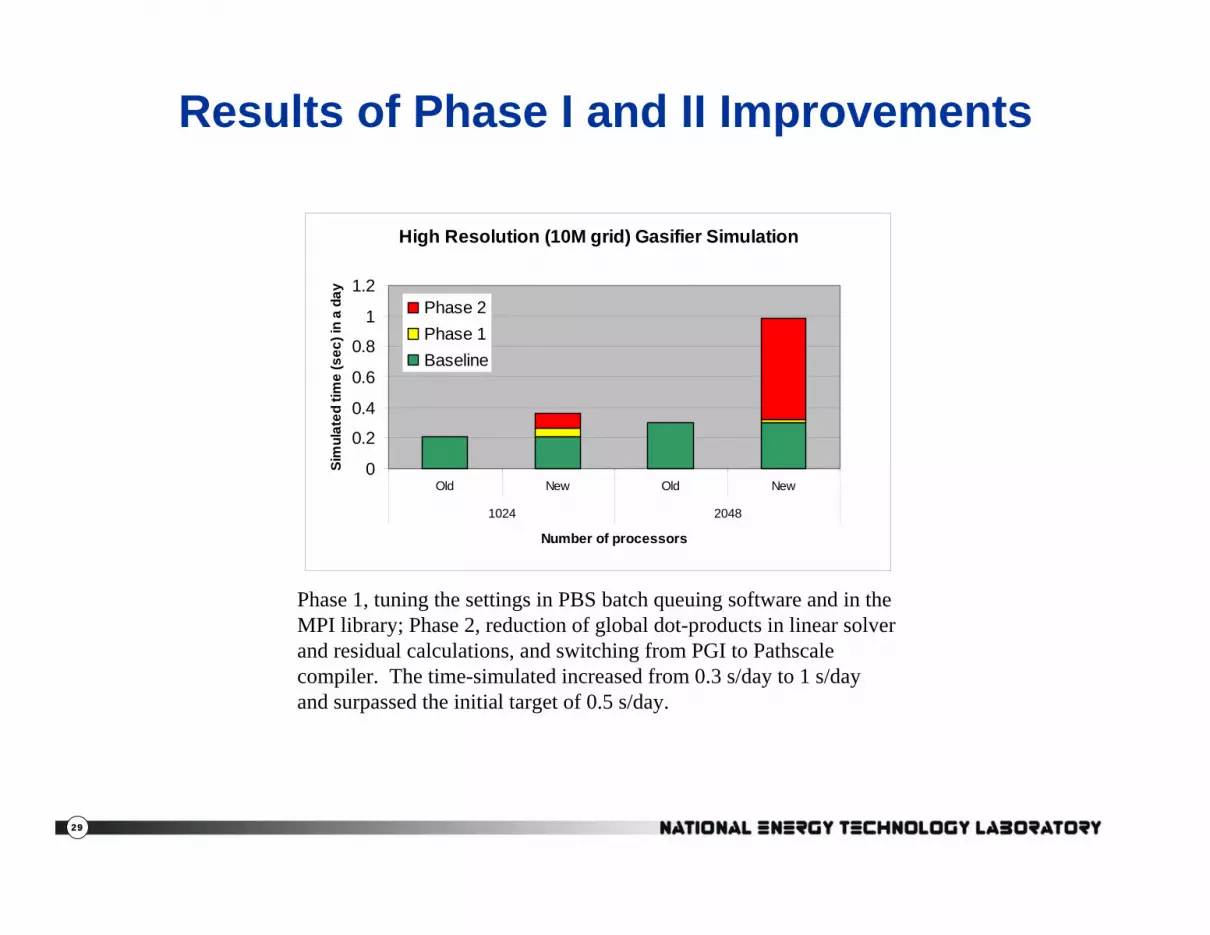
Results of Phase I and II Improvements

Phase 1, tuning the settings in PBS batch queuing software and in the MPI library; Phase 2, reduction of global dot-products in linear solver and residual calculations, and switching from PGI to Pathscalecompiler. The time-simulated increased from 0.3 s/day to 1 s/day and surpassed the initial target of 0.5 s/day.

High Resolution (10M grid) Gasifier Simulation

0

0.2

0.4

0.6

0.8

1

1.2

Old New Old New

1024 2048

Number of processors

Sim

ulat

ed ti

me

(sec

) in

a da

y

Phase 2Phase 1Baseline

30

CrayPAT report on time spent for MPI

• …..• | 22.0% | 136.579381 | -- | -- | 96745.0 |MPI_SYNC• ||-----------------------------------------------------------------• || 8.9% | 55.230971 | 28.237006 | 33.9% | 96319.0 |mpi_allreduce_(sync)• || 6.1% | 37.847392 | 2.383306 | 5.9% | 37.0 |mpi_scatterv_(sync)• || 6.0% | 37.142502 | 4.099108 | 9.9% | 66.0 |mpi_gatherv_(sync)• ||========================================================

• | 8.7% | 53.941060 | -- | -- | 834159.9 |MPI• ||-----------------------------------------------------------------• || 3.1% | 19.234665 | 1.928393 | 9.1% | 96319.0 |mpi_allreduce_• || 2.7% | 16.654918 | 59.893473 | 78.3% | 360682.0 |mpi_waitall_• || 1.7% | 10.544340 | 1.269582 | 10.8% | 356668.0 |mpi_startall_• |========================================================

31

Points about OpenMP to ponder

!$omp do parallel around loops are the easiest to implement, but not the best for performanceOne global !$omp parallel along with !$omp master and !$omp do perform better, but are not easy to code and maintain

On a XT5 node, memory has affinity to the process where it is first referenced. If all memory has affinity to thread 0, then both sockets are accessing the same memory.

32

Coal Combustion/Gasification

• Devolatilization

• Cracking• Drying• Water-gas shift reaction• Gasification Combustion

HF: Volatile Matter d Tar + dCOCO + d

CO2CO2 + dCH4CH4 + d

H2H2 + dH2OH2O

IF: Tar cC + cCOCO + c

CO2CO2 + cCH4CH4 + c

H2H2 + cH2OH2O

GF: Moisture (coal) H2O

EF: CO + H2O CO2 + H2

BF: C + H2O CO + H2

CF: C + CO2 2CO

DF: ½C + H2 ½CH4

AF: 2C + O2 2CO

2F: CO + ½O2 CO2

1F: CH4 + 2O2 CO2 + 2H2O

0F: H2 + 2O2 H2O

33