Adaptive Bolus Chasing Computed Tomography Angiography:Control Scheme and Experimental Results

Zhijun Cai1, Colbin Erdahl1, Kai Zeng2, Tom Potts1, Melhem Sharafuddin3, Osama Saba4,Ge Wang5, and Er-Wei Bai11Department of Electrical and Computer Engineering, University of Iowa, Iowa City, IA, 522422Department of Biomedical Engineering, University of Iowa, Iowa City, IA, 522423University of Iowa Hospital and Clinic, University of Iowa, Iowa City, IA, 522424Siemens Medical Solutions, Iowa City, IA, 522425VT-WFU School of Biomedical Engineering & Sciences, Virginia Polytechnic Institute & StateUniversity, Blacksburg, VA 24061, USA

AbstractIn this paper, a new adaptive bolus-chasing control scheme is proposed to synchronize the bolus peakin a patient’s vascular system and the imaging aperture of a computed tomography (CT) scanner.The proposed control scheme is theoretically evaluated and experimentally tested on a modifiedSiemens SOMATOM Volume Zoom CT scanner. The first set of experimental results are reportedon bolus-chasing CT angiography using realistic bolus dynamics, real-time CT imaging and adaptivetable control with physical vasculature phantoms. The data demonstrate that the proposed controlapproach tracks the bolus propagation well, and clearly outperforms the constant-speed scheme thatis the current clinical standard.

KeywordsAdaptive bolus chasing; Computed Tomography Angiography

I. IntroductionWith the advent of the multi-slice CT scanner, CT Angiography (CTA) has become animportant investigative tool for vascular diseases such as aneurysms and atherosclerosis[1-4]. It produces cross-sectional images of arteries throughout the body in a fast and minimallyinvasive way. To better define the vasculature from its surrounding soft tissue, a dose of contrastmedium (a bolus) is usually injected into a vein through an IV (intravenous) tube. During thescanning, the patient lies on the CT table. The table is translated into the CT gantry, and thepart of the patient’s body which is under the x-ray aperture is scanned at that time. In themeantime, the contrast bolus propagates along the blood vessel. Consequently, synchronizationof the CT imaging aperture and the contrast bolus peak would result in CT images with a higherContrast to Noise Ratio (CNR).

© 2008 Elsevier Ltd. All rights reserved.Publisher's Disclaimer: This is a PDF file of an unedited manuscript that has been accepted for publication. As a service to our customerswe are providing this early version of the manuscript. The manuscript will undergo copyediting, typesetting, and review of the resultingproof before it is published in its final citable form. Please note that during the production process errors may be discovered which couldaffect the content, and all legal disclaimers that apply to the journal pertain.

NIH Public AccessAuthor ManuscriptBiomed Signal Process Control. Author manuscript; available in PMC 2009 October 1.

Published in final edited form as:Biomed Signal Process Control. 2008 October ; 3(4): 319–326. doi:10.1016/j.bspc.2008.04.005.

NIH

-PA Author Manuscript

NIH

-PA Author Manuscript

NIH

-PA Author Manuscript

The problem, however, is that the contrast bolus dynamics are highly nonlinear, complicated,and influenced by many factors, e.g., patient weight, vasculature diseases, and injectionpatterns. In current practice, the CT table moves at a preset constant speed, and is very likelyto miss the bolus peak. To compensate for this problem, a large amount of contrast medium isinjected, which is harmful to the patient’s kidney.

To overcome the above problem, the timing bolus [5-7] and ROI (Region Of Interest) thresholdtriggering [8] methods have been proposed for a long time. Both methods endeavor to providea “correct” time to start the CT table. The former method uses a small amount of the test contrastbolus to obtain the bolus arrival time at the ROI, which is then used to start the CT table forthe normal scan. However, the arrival time for the test bolus and the main bolus may not beconsistent because of different injection volumes and complicated bolus dynamics. The lattermethod presets a threshold for a selected ROI, and starts to move the CT table when the bolusdensity inside the ROI reaches this threshold. This is also questionable because the optimalthreshold is not known a priori. When the threshold is set too low, the CT table starts too early,and when it is set too high, the CT table does not start at all. A fundamental problem for bothmethods is that they move the CT table at a constant velocity which does not match the varyingbolus velocity during the propagation.

Another class of approaches to obtain the high-CNR CT images tries to optimize the bolusgeometry by means of varying the injection rate and duration [8-15]. It is expected that if abolus keeps its maximum density for a longer time at a position, then it is easier to synchronizethe CT imaging aperture and the bolus peak. As a result, many injection protocols werereported. The multiple-injection method [15] injects the bolus at varying rates; the inversemethod [16] obtains the injection protocol (input) from the desired output (the optimized bolusgeometry) by taking the system as a LTI (Linear Time-Invariant) system. These approachesneed a test bolus and/or a LTI system assumption, which is far away from the reality. Inaddition, the geometry optimization method may end up with a larger amount of contrast dose,which is not good for patients.

To make it clear, in the following texts “bolus chasing” means to track the bolus throughoutthe scan by means of varying the table speed, not just to chase the bolus arrival. The boluschasing techniques were studied in Digital Subtraction Angiography (DSA) [17,18] andMagnetic Resonance Angiography (MRA) [19-22]. Preferable results have been reported inthese studies. However, there are few studies on bolus chasing CTA [23]. The reason for thisis that CTA has a much smaller field of view (z direction) compared to DSA or MRA, and theCT image reconstruction algorithm for varying pitch is complicated.

Recently, we have developed the CT image reconstruction algorithms for varying pitch [24]and investigated the bolus characteristic from hundreds of clinical bolus datasets [26]. We havealso developed an adaptive bolus chasing control schemes and numerically tested it on clinicalbolus datasets [25]. To the best of our knowledge, no experimental result has ever been reportedin the literature on bolus chasing CTA. In this paper, we report the experimental results of thecontrol schemes on a Siemens SOMATOM Volume Zoom CT scanner. Although theexperiments are conducted on phantoms, results have successfully shown that the proposedcontrol scheme works very well.

The layout of the paper is as follows. Bolus propagation model and problem statement areintroduced in Section II. Section III describes the experimental setup. Section IV presents theapproach to the problem. Then in Section V, the experimental results are given. Conclusionsare provided in Section VI.

Cai et al. Page 2

Biomed Signal Process Control. Author manuscript; available in PMC 2009 October 1.

NIH

-PA Author Manuscript

NIH

-PA Author Manuscript

NIH

-PA Author Manuscript

II. Bolus propagation model and problem statementIn this section, we discuss the bolus propagation model and formally state the bolus chasingproblem.

Bolus propagation modelAfter the injection, the contrast bolus propagates and disperses in the blood vessel. Its densityvaries with time and distance (z direction). Due to the limited FOV (Field Of View) of CTA,it is not practical to obtain the bolus density information over a long distance. Many researchershave described the bolus using temporal profiles at several positions, such as the aorta and theliver [9,10,27]. Blomley and Dawson [28] suggested a Gamma function to depict the bolustime-attenuation profile at the aorta, and earlier, Stow and Hetzel [29] proposed an empiricalformula for the bolus temporal curve. Probably the most well known temporal profile is thelagged normal density model reported by Bassingthwaighte in [30]. This model is able to fitthe bolus curve for a wide range of cases. In our previous work [25], we fitted the bolus datato the lagged normal density model for a wide range of cases in the aorta, and as a result andwe were able to obtain the bolus velocity in the aorta according to those profiles.

Although there are many models to describe the bolus temporal behavior at a position, acommon property is that the bolus time-density curve is more or less like a bell for a singleinjection [9,10,25]. In other words, the bolus density is monotonically increasing anddecreasing before and after reaching its maximum density, respectively. Based on this feature,we have designed an optimal adaptive control scheme for bolus chasing CTA [26]. Thenumerical simulation results based on the clinical data have shown that the adaptive boluschasing control scheme outperforms the constant speed method substantially.

Problem statementThe control objective is to keep the peak of the moving bolus right under the x-ray aperture.This is achieved by instantaneously processing the bolus CT image on the monitor, dynamicallypredicting the bolus peak position at the next sampling time, and adaptively moving the CTtable in the opposite direction to follow the bolus peak.

III. Experimental setupIn this section, the experimental setup is introduced, and some key parts are elaborated. Figure1 is a photo of the experimental setup. The pump system, plastic tube filled with water andreservoirs are all placed on the CT table and used to simulate the blood system. When the pumpis turned on, it drives the bolus inside the tube. The bolus velocity can be changed by varyingthe pump speed. During the scan, the bolus cross-sectional image is shown on the monitor byreal time image reconstruction algorithms. A frame grabber is used to capture the CT imagesand feed the bolus information to the controller. The controller predicts the bolus peak positionat the next sampling time, and sends a command to move the table accordingly. Thus, the boluspeak is kept right under the CT imaging aperture.

CT scannerThe CT scanner is a Siemens SOMATOM Volume Zoom four-slice CT scanner with softwareversion A40A. Table 1 shows some critical technical parameters:

Siemens has also provided us with the CANbus access and command format in order to controlthe CT table.

Cai et al. Page 3

Biomed Signal Process Control. Author manuscript; available in PMC 2009 October 1.

NIH

-PA Author Manuscript

NIH

-PA Author Manuscript

NIH

-PA Author Manuscript

Frame grabberAlthough we have the CT reconstruction algorithm for varying pitch, we are not able toreconstruct the CT images due to the unavailability of the proprietary raw data. Therefore, theonly possible feedback of the bolus density is the real time CT image on the monitor. To thatend, we split the CT VGA signal, feed it to the controller, and capture it using a frame grabber.The frame grabber, manufactured by the NCast Corporation(http://www.ncast.com/DigiCaptureCard.html), is a Digitizer 3.0 Capture Card. It supportsstandard VGA input modes with a frequency of up to 85Hz and a maximum resolution of 1280×1024, and is able to capture the image signal at a speed of 30 frames per second.

Pump systemThe blood vascular system is physically simulated by a programmable MasterFlex pumpsystem (HV-07523-60 L/S Brushless Digital Drives, made by the Cole Parmer Company,http://www.masterflex.com) connected to a plastic tube filled with water. By changing thepump head size and speed, the water flow rate can be varied between 0.6 and 3400 mL/min.During the experiment, we adjust the pump speed to achieve the desirable bolus dynamics.Roughly speaking, the bolus speed is proportional to the pump flow rate, though in reality itis not exactly proportional because of the irregularity of the tube and discontinuity of the flow.

Delay issuesAs mentioned before, we have limited access to the CT scanner, which gives us two delays:an image display delay and a control delay. The image display delay is caused by the imagereconstruction and display on the monitor. In this experiment, we used the CAREVision mode,and the image display delay is about 0.79 seconds. That is to say that when a target is sent intothe CT gantry right under the x-ray aperture, its CT image will be shown on the monitor 0.79seconds later. The other delay is the control delay, which is actually a combination of twodelays caused by CANbus communication and table movement execution. In the CT CANbussystem provided by Siemens, the CANbus decodes and encodes at rate of 100Kbps and takesa minimum of 100ms for transmitting or receiving a command. The table movement executiondelay is the time needed to move the CT table from one position to another, and that dependson the length and speed of the movement. The combined delay is variable depending on theCANbus activity, the speed at which the controller can process the data, and the number ofdata bits in the message. To that end, we must wait for a certain time (CANbus command delayplus table moving time) between two consecutive CANbus commands, or the CT scannerwould abandon the current scan and jump out of CAREVison mode. We have measured thatthe CANbus command delay is about 0.15 seconds on this CANbus system. The combineddelay can be as high as 1.3-2 seconds. The translation is that once a control command is fed tothe CANbus, the next control command can only be sent out after 1.3-2 seconds. This poses avery serious challenge for controller design. It is important to comment that the combinedcontrol delay is caused by the CANbus. If the full proprietary control commands are availableto us, the control delay problem is nonexistent. We are currently working with Siemens to tryto have those full proprietary control commands in the near future. All the results reported inthis paper are under the control delay constraint.

IV. ApproachIdeally, we would like to be able to send CT table control commands continuously so that theCT table can follow the bolus peak continuously. Because of the delays, especially thesignificant control delay, the ability to follow a bolus with arbitrary dynamics is severelylimited. Therefore, in the presence of a control delay, the bolus dynamics, including themaximum speed and the maximum acceleration, have to be scaled down to within theconstraints imposed by the delays. Scaling down the bolus speed and acceleration can be done

Cai et al. Page 4

Biomed Signal Process Control. Author manuscript; available in PMC 2009 October 1.

NIH

-PA Author Manuscript

NIH

-PA Author Manuscript

NIH

-PA Author Manuscript

easily by simply changing the pump flow. However, scaling down the bolus dispersion is notpossible. To this end, in our experiments, we use a solid aluminum bolus immersed in the waterinstead of the actual liquid bolus. The temporal profile of the solid bolus is made to resemblethe actual bell-shaped bolus. The dispersed bolus density is represented by the solid boluscross-sectional area, and the bolus peak position is the center of the solid bolus. The basic ideaof bolus chasing is to combine image feedback and control. The feedback information of thebolus dynamics is obtained from imaging reconstruction algorithms and is then used to guidethe control. The experiment using a solid bolus should serve its purpose, i.e., it should be ableto tell whether the idea of combining imaging and control is feasible. In fact, tracking a solidbolus with the length of about 40mm can actually be tougher than tracking a liquid bolus. Abolus about 40mm long is easily missed by the x-ray aperture if the CT table does not followthe bolus peak closely. Once missed, it is very hard to re-capture it because no feedbackinformation on the bolus is available. On the other hand, because of dispersion, a liquid bolusis much longer and relatively easy to follow.

We now design a simple yet effective algorithm to track the bolus peak with the presence ofthe delays. The following notations will be used throughout the paper.

Tk Tk = kΔT, where ΔT is the time interval between two consecutive control commands.

Z(k) Table position at time Tk.

B(k) Bolus peak position at timeTk.

E(k) Error between table position and bolus peak at time Tk, E(k) = B(k) - Z(k).

α Control gain.

Den(k) Observed bolus density at time Tk.

l Number of steps in the length of the display delay.

Assuming that the display delay is lΔT which means that at time Tk=kΔT, the controller onlyhas the bolus peak information up to time (k-l)ΔT. The next CT table position Z(k+1) ispredicted as the combination of three components: 1) the current position of the CT table Z(k), which is available; 2) the difference between the two consecutive bolus peak positions attimes (k-l)ΔT and (k-l-1)ΔT; and 3) the calculated error between the bolus peak position andthe CT table position at time (k-l)ΔT. Theorem 1 states the control law for the case when thebolus moves linearly.

Theorem 1If the bolus is bell shaped as discussed above and moves at a constant speed, i.e., B(k)=B(k-1)+Δ, for some constant Δ>0, consider the following control law for some integer l>0,

(1)

where E(k)=B(k)-Z(k). Then, there exists αmax(l)>0, such that for all 0<α<αmax(l), the closedloop system is exponentially stable, or equivalently, the error E(k) goes to zero asymptotically.

ProofThe error dynamics are given as

Cai et al. Page 5

Biomed Signal Process Control. Author manuscript; available in PMC 2009 October 1.

NIH

-PA Author Manuscript

NIH

-PA Author Manuscript

NIH

-PA Author Manuscript

The characteristic equation is

Then for each integer l, there exists αmax(l)>0 so that for all 0<α<αmax(l) the closed loop system

is exponentially stable, which implies .■

Theorem 2 characterizes the performance of the control law when the bolus moves in anonlinear fashion. The proof is similar and is omitted.

Theorem 2Suppose the bolus is bell shaped as discussed and B(k)=B(k-1)+Δk, and |Δi-Δi-l|≤ ε, for ∀1≤i≤l. Then, considering the control law (1) with the same control gainα, the tracking error ofthe closed loop system is bounded by

Since the image display delay is much smaller than ΔT, which is determined by the controldelay, l=1 in all our experiments. The results, however, apply equally to any integer l.

Bolus profile and tracking errorTo determine the tracking error in control law (1), we first obtain the bolus density profilebefore the experiment, and then approximate it by a 2nd order polynomial. The tracking erroris obtained through the approximated polynomial and the online scanned density. To determinethe bolus profile, we scan the bolus under the CAREVision mode (the same mode to implementthe controller), and set the CT window center and width as 1500 Hounsfield Units (HU) and500 HU, respectively. Thus, only the bolus is shown on the screen, because the aluminum hasa CT number greater than 2000 HU, and the background is black. The bolus inside the plastictube is fed into the gantry with water driven by the pump at a speed of 1mm/sec, and at thesame time, the bolus CT images are captured by the frame grabber every 0.15 seconds. Thus,we can extract the bolus density from the VGA signal, which has a range of 0∼255. Recall thatour settings of the CT window center and width make the bolus almost white with a blackbackground. Therefore, the bolus cross-sectional area is white on the screen. Further, we denotethe bolus density by the number of pixels that are greater than a threshold. The threshold valueis set to be 50 in order to account for all the pixels of the bolus. Figure 2 shows the bolus densityprofile. Let Zmax and Zmin be the bolus maximum and minimum positions in the z direction,and Zc denote the bolus center or peak position. The bolus density at any position z can beapproximated by

where A and C are constants.

Cai et al. Page 6

Biomed Signal Process Control. Author manuscript; available in PMC 2009 October 1.

NIH

-PA Author Manuscript

NIH

-PA Author Manuscript

NIH

-PA Author Manuscript

At time Tk, the table position is Z(k), and the measured bolus density is Den (k )>0. Assumethat the bolus center is B(k) at that time. By substituting B(k) for Zc and Z(k) for z, we have

(2)

Consequently, we are able to obtain the magnitude of the tracking error E(k) by

(3)

The next step is to determine the sign of the tracking error, because the observed density doesnot tell us whether the bolus center is ahead of or behind the x-ray aperture. A simple conceptis shown in Figure 3. When the CT table is stopped, the bolus will be moving forward throughthe aperture. Thus, we will measure an increasing bolus density (Measurements 1 and 2) if thex-ray is scanning the head of the bolus (negative error). On the other hand, the decreasingmeasurement readings (Measurements 3 and 4) indicate that the bolus tail is being scanned(positive error). In practice, we take nine measurements, and determine the error sign by theslope of these densities to reduce the noise effect.

Remarks—

1. The table must be stopped while taking the measurements; otherwise the aboveargument is not valid. If the table moves faster in the opposite direction of the bolus,the error sign will be positive for measurements 1 and 2, and negative formeasurements 3 and 4. Besides this, the table has to be stopped after a move to ensurethat the CANbus command has been completely executed.

2. At the peak of the bolus, the error sign can easily be determined erroneously in thepresence of noise, because the bolus density is more or less flat there, and a smallchange affects the determination of the sign. Fortunately, in this scenario, themagnitude of the error is small, which results in little movement, and does not havea noticeable impact.

Control procedureFigure 4 is the flow chart of the bolus chasing CTA control procedure. The controller startswhen the observed bolus density exceeds some preset threshold. Unlike the constant speedmethod, in the bolus chasing method, the controller being activated does not mean that the CTtable moves forward right away. The speed and length of the next table movement depend onthe measured bolus density. The tracking procedure is over when the CT has scanned theprescribed length. This is consistent with current clinical practice, where a length is pre-definedbefore a CT examination [4].

Because of the delay issues, it is critical to guarantee that we measure the bolus density duringthe time that the table is temporally stopped, and there is enough waiting time between twoconsecutive commands. Figure 5 shows the time arrangement for table moving, waiting, andimage delay in one step. In Figure 5, the table moving time in one step is 0.7 seconds, and theimage capturing time is about 0.35 seconds. It is easy to see that image capturing commandsare sent while the table is stopped.

Cai et al. Page 7

Biomed Signal Process Control. Author manuscript; available in PMC 2009 October 1.

NIH

-PA Author Manuscript

NIH

-PA Author Manuscript

NIH

-PA Author Manuscript

Dealing with the stopped bolusIn reality, when the bolus meets an aneurysm, or in certain other situations, it may stay therefor a while before it moves again. To that end, the control law has to be modified, because thestatic bolus produces almost the same measurements and could result in a wrong trackingdirection. Fortunately, we know that when the bolus is stopped, the variance of densitymeasurements is small (we take nine measurements for each step), while the moving bolusgives a very big variance. Therefore, we say that if the density variance is small and the averagedensity is in some range, then the bolus is stopped, and we move the table to its peak.

Remarks—

1. It is not suggested to move a big step while the bolus has been detected to be stopped,because the table may move the bolus across its peak and give a wrong error sign.

2. To detect whether or not the bolus is stopped, we need to check if the average densityis close to the maximum, because when we are tracking on the bolus peak, the varianceis also very small.

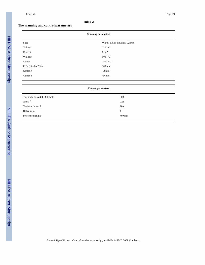
V. Experimental resultsThe experimental parameters are in Table 2.

In order to show the controller’s ability to track the bolus with different dynamics, weprogrammed the pump for three kinds of patterns: constant bolus speed, exponentiallydecreasing bolus speed, and piecewise constant bolus speed. It is important to emphasize thatthe pump speed only roughly represents the bolus velocity, which is not known exactlythroughout the experiment.

Constant bolus speedFor this experiment, the pump is running at 150 rpm all the time. The tracking results are shownin Figure 6, where the top plot shows the CT table movement trajectory, and the bottom plotshows the observed density at each time. We can see that the CT table starts before the 10th

second, when the observed density exceeds the threshold. Most of the measured densities aregreater than 2000, which is very close to the maximum. The reason that there are a couple ofpoints that have a value less than 1500 is that the bolus does not move constantly in the plastictube due to the irregularity of the tube and the discontinuous pump output flow. Although wementioned that the bolus velocity is not available throughout the experiment, we can tell thebolus trajectory roughly from Figure. 6. If the scanned bolus density is very close to themaximum, it means that we are tracking the bolus center well.

Exponentially decreasing bolus speedThe actual bolus in a human body does not flow constantly inside the blood vessel. It is reportedthat the blood flows slower in the artery when it is further away from the heart. For a normalmale adult, the average blood velocity in the aorta is about 27cm/sec, while it is around 10cm/sec in the common femoral artery. To this end, we reduce the pump speed while the bolus ismoving. The pump speed obeys the equation Vp(t)=(125-90)e-0.01t+110, where Vp(t) is thepump speed with unit rpm.

Figure 7 shows the experimental results for tracking the bolus driven by exponentiallydecreasing speed. In Figure 7, the top plot is the table movement and the bottom plot gives thescanned bolus density at each time step. Again, most of the measured densities are greater than1500. It is noted that the scanned bolus density is jiggling all the time. The reason for this isthat the pump speed is decreasing all the time, and the bolus does not flow constantly at all.

Cai et al. Page 8

Biomed Signal Process Control. Author manuscript; available in PMC 2009 October 1.

NIH

-PA Author Manuscript

NIH

-PA Author Manuscript

NIH

-PA Author Manuscript

However, the controller is able to track the bolus well even if the bolus flows nonlinearly,provided that the bolus speed does not change too much.

Variable bolus speedThe bolus may stay in the same place for a while and then move again in some cases, such asan aneurysm. To simulate that, we reduce the pump speed to stop/slow the bolus for some time.Figure 8 is the pump speed profile, which shows that the pump runs at 90 rpm between 35 and60 seconds, and 150 rpm before and after that period. The tracking results are shown in Figure9, where the top plot shows the CT table movement trajectory, and the bottom plot shows theobserved density. It is noticeable that the controller tracks the bolus well even when it is almoststatic between 35 and 60 seconds.

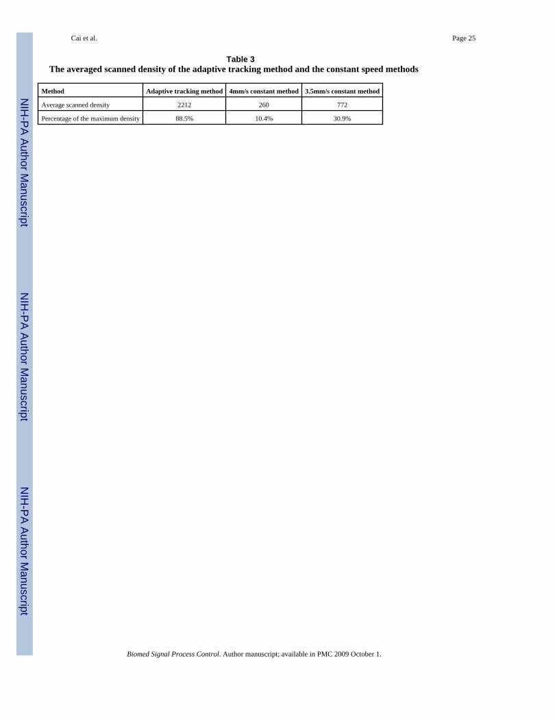
To compare the adaptive chasing method with the current constant CT table speed method, wescan the bolus with two different constant table speeds: 4mm/s and 3.5 mm/s. As we expect,results are unsatisfactory (see the bottom plot of Figure 10). The CT table that moves at aconstant speed of 4mm/s only catches the bolus at the very beginning, and loses the bolus after40 seconds, while the table moving at 3.5mm/s catches the bolus thrice and only scans thebolus peak for a few seconds. To make a quantitative comparison, we compute the averagescanned densities over the scanning duration for both the adaptive chasing method and theconstant CT table speed method, along with their percentages of the maximum density (2500)as shown in Table 3. It is clear that the adaptive chasing method follows close to the bolus peak(88.5%), while the constant CT table methods have poor performances, 10.4% and 30.9% for4mm/s and 3.5mm/s, respectively.

Based on the normalized scanned bolus density, we reconstruct the 3D plastic tubes, whichrepresent blood vessels, and are shown in Figure 11, where the left, middle and right “bloodvessels” are reconstructed using the data for the adaptive tracking method, the 4mm/s constantCT table method, and the 3.5 mm/s method, respectively. Obviously, the 3D “blood vessel”based on the adaptive tracking method is fully reconstructed, while the constant CT table speedmethods do not show the whole “blood vessel”. The reason for this is that the adaptive chasingmethod scanned the “blood vessel” from the beginning to the end with the peak of the bolusof contrast, while the constant speed methods did not.

VI. Concluding remarksIn this paper, we proposed a control scheme to track the contrast bolus using the feedback fromreal time CT images. Although the experiments were conducted on phantoms, the experimentalresults have shown that 1) the proposed scheme tracks the bolus center well (88.5% of the peakdensity), despite the delays in the system; 2) the adaptive tracking method outperforms theconstant table speed method by a factor of 2.8 or more.

It is the first experiment result reported as we are aware of for adaptive bolus chasing CTA. Inthe near future, we will replace the tube with more realistic vasculature phantom, and programthe pump to have an output of the real human heart. Eventually, we will apply this adaptivetracking method on the patient in clinic who needs an exam of the Computed TomographyAngiography.

Reference1. Fleischmann D, Hallett RL, Rubin GD. CT angiography of peripheral arterial disease. J Vasc Interv

Radiol 2006;17(1):3–26. [PubMed: 16415129]

Cai et al. Page 9

Biomed Signal Process Control. Author manuscript; available in PMC 2009 October 1.

NIH

-PA Author Manuscript

NIH

-PA Author Manuscript

NIH

-PA Author Manuscript

2. Ofer A, Nitecki SS, et al. Multidetector CT angiography of peripheral vascular disease: a prospectivecomparison with intraarterial digital subtraction angiography. AJR Am J Roentgenol 2003;180(3):719–24. [PubMed: 12591682]

3. Chow LC, Rubin GD. CT angiography of the arterial system. Radiol Clin North Am 2002;40(4):729–49. [PubMed: 12171182]

4. Van Hoe L, Gryspeerdt S, et al. Spiral CT angiography. J Belge Radiol 1995;78(2):114–7. [PubMed:7601813]

5. van Hoe L, Marchal G, et al. Determination of scan delay time in spiral CT-angiography: utility of atest bolus injection. J Comput Assist Tomogr 1995;19(2):216–20. [PubMed: 7890844]

6. Puls R, Knollmann F, et al. Multi-slice spiral CT: 3D CT angiography for evaluating therapeuticallyrelevant stenosis in peripheral arterial occlusive disease. Rontgenpraxis 2001;54(4):141–7. [PubMed:11883117]

7. Bae KT. Test-bolus versus bolus-tracking techniques for CT angiographic timing. Radiology 2005;236(1):369–70. [PubMed: 15987987]author reply 370

8. Schweiger GD, Chang PJ, Brown BP. Optimizing contrast enhancement during helical CT of the liver:a comparison of two bolus tracking techniques. AJR Am J Roentgenol 1998;171(6):1551–8. [PubMed:9843287]

9. Bae KT, Heiken JP, Brink JA. Aortic and hepatic peak enhancement at CT: effect of contrast mediuminjection rate--pharmacokinetic analysis and experimental porcine model. Radiology 1998;206(2):455–64. [PubMed: 9457200]

10. Cademartiri F, van der Lugt A, et al. Parameters affecting bolus geometry in CTA: a review. J ComputAssist Tomogr 2002;26(4):598–607. [PubMed: 12218827]

11. Claussen CD, Banzer D, et al. Bolus geometry and dynamics after intravenous contrast mediuminjection. Radiology 1984;153(2):365–8. [PubMed: 6484168]

12. Kirchner J, Kickuth R, et al. Optimized enhancement in helical CT: experiences with a real-time bolustracking system in 628 patients. Clin Radiol 2000;55(5):368–73. [PubMed: 10816403]

13. Kopka L, Rodenwaldt J, et al. Dual-phase helical CT of the liver: effects of bolus tracking and differentvolumes of contrast material. Radiology 1996;201(2):321–6. [PubMed: 8888218]

14. Rist C, Nikolaou K, et al. Contrast bolus optimization for cardiac 16-slice computed tomography:comparison of contrast medium formulations containing 300 and 400 milligrams of iodine permilliliter. Invest Radiol 2006;41(5):460–7. [PubMed: 16625109]

15. Rossi P, Baert A, et al. Multiple bolus technique vs. single bolus or infusion of contrast medium toobtain prolonged contrast enhancement of the pancreas. Radiology 1982;144(4):929–31. [PubMed:7111749]

16. Fleischmann D, Hittmair K. Mathematical analysis of arterial enhancement and optimization of bolusgeometry for CT angiography using the discrete fourier transform. J Comput Assist Tomogr 1999;23(3):474–84. [PubMed: 10348458]

17. Fritschy P, Terrier F. Intravenous digital subtraction angiography of the lower extremities combinedwith step translation (2-field DSA). Rofo 1988;148(3):279–84. [PubMed: 2832892]

18. Wu, Z.; Qian, J. IEEE Workshop on Biomedical Image Analysis. Santa Barbara, CA: 1988. Real-time tracking of contrast bolus propagation in X-ray peripheral angiography.

19. Wang Y, Lee HM, et al. Bolus-chase MR digital subtraction angiography in the lower extremity.Radiology 1998;207(1):263–9. [PubMed: 9530326]

20. Kruger DG, Riederer SJ, et al. Dual-velocity continuously moving table acquisition for contrast-enhanced peripheral magnetic resonance angiography. Magn Reson Med 2005;53(1):110–7.[PubMed: 15690509]

21. Ho VB, Choyke PL, et al. Automated bolus chase peripheral MR angiography: initial practicalexperiences and future directions of this work-in-progress. J Magn Reson Imaging 1999;10(3):376–88. [PubMed: 10508299]

22. Hany TF, Carroll TJ, et al. Aorta and runoff vessels: single-injection MR angiography with automatedtable movement compared with multiinjection time-resolved MR angiography--initial results.Radiology 2001;221(1):266–72. [PubMed: 11568351]

23. Bennett J, Bai E, et al. A Preliminary Study on Adaptive Field-of-View Tracking in Peripheral DigitalSubtraction Angiograph. J. of X-ray Science and Technology 2003;11:149–159.

Cai et al. Page 10

Biomed Signal Process Control. Author manuscript; available in PMC 2009 October 1.

NIH

-PA Author Manuscript

NIH

-PA Author Manuscript

NIH

-PA Author Manuscript

24. Yu H, Ye Y, et al. A backprojection-filtration algorithm for nonstandard spiral cone-beam CT withan n-PI-window. Phys Med Biol 2005;50(9):2099–111. [PubMed: 15843739]

25. Cai Z, Stolpen A, et al. Bolus characteristics based on Magnetic Resonance Angiography. BiomedEng Online 2006;5:53. [PubMed: 17044929]

26. Bai E-W, Cai Z, et al. An Adaptive Optimal Control Design for a Bolus Chasing ComputedTomography Angiography. IEEE Transction on Control System Technology. 2006

27. Qanadli SD, Mesurolle B, et al. Abdominal aortic aneurysm: pretherapy assessment with dual-slicehelical CT angiography. AJR Am J Roentgenol 2000;174(1):181–7. [PubMed: 10628476]

28. Blomley MJ, Dawson P. Bolus dynamics: theoretical and experimental aspects. Br J Radiol 1997;70(832):351–9. [PubMed: 9166070]

29. Stow RW, Hetzel PS. An empirical formula for indicator-dilution curves as obtained in human beings.J Appl Physiol 1954;7(2):161–7. [PubMed: 13211491]

30. Bassingthwaighte JB, Ackerman FH, Wood EH. Applications of the lagged normal density curve asa model for arterial dilution curves. Circ Res 1966;18(4):398–415. [PubMed: 4952948]

Cai et al. Page 11

Biomed Signal Process Control. Author manuscript; available in PMC 2009 October 1.

NIH

-PA Author Manuscript

NIH

-PA Author Manuscript

NIH

-PA Author Manuscript

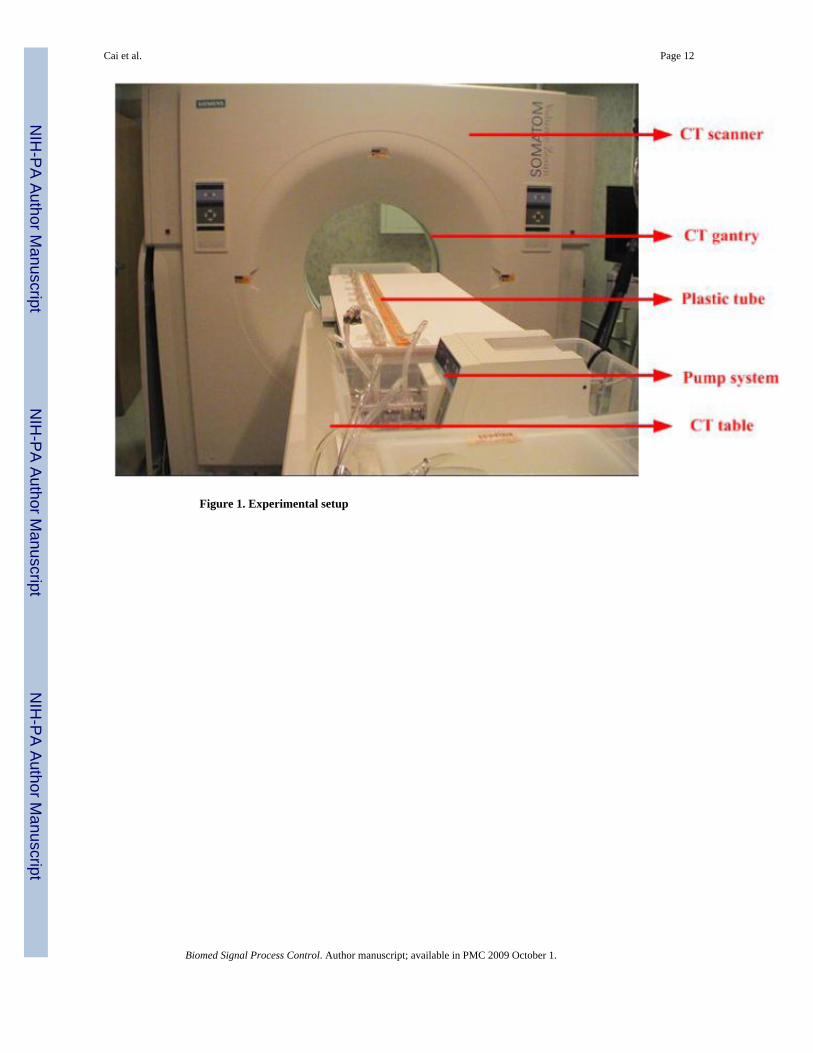
Figure 1. Experimental setup

Cai et al. Page 12

Biomed Signal Process Control. Author manuscript; available in PMC 2009 October 1.

NIH

-PA Author Manuscript

NIH

-PA Author Manuscript

NIH

-PA Author Manuscript

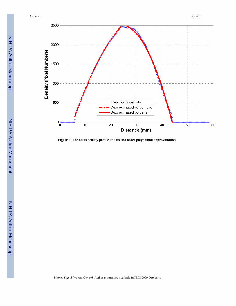
Figure 2. The bolus density profile and its 2nd order polynomial approximation

Cai et al. Page 13

Biomed Signal Process Control. Author manuscript; available in PMC 2009 October 1.

NIH

-PA Author Manuscript

NIH

-PA Author Manuscript

NIH

-PA Author Manuscript

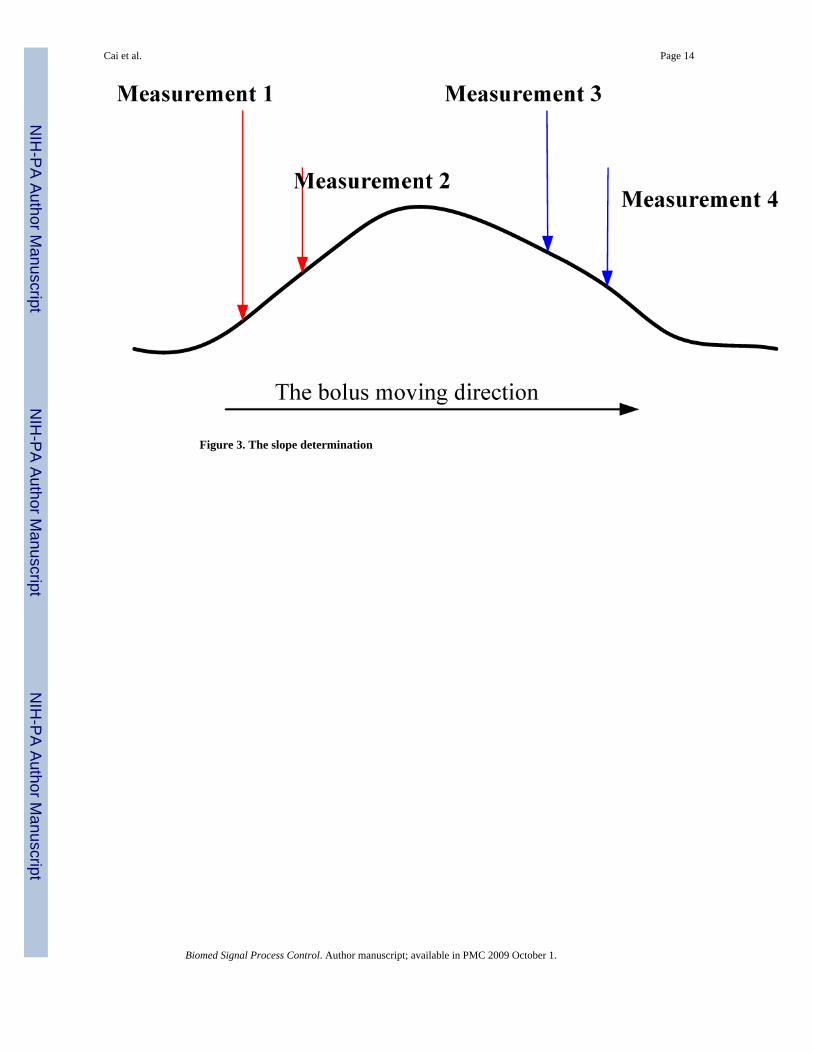
Figure 3. The slope determination

Cai et al. Page 14

Biomed Signal Process Control. Author manuscript; available in PMC 2009 October 1.

NIH

-PA Author Manuscript

NIH

-PA Author Manuscript

NIH

-PA Author Manuscript

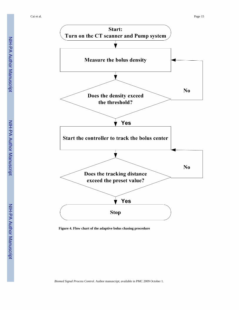
Figure 4. Flow chart of the adaptive bolus chasing procedure

Cai et al. Page 15

Biomed Signal Process Control. Author manuscript; available in PMC 2009 October 1.

NIH

-PA Author Manuscript

NIH

-PA Author Manuscript

NIH

-PA Author Manuscript

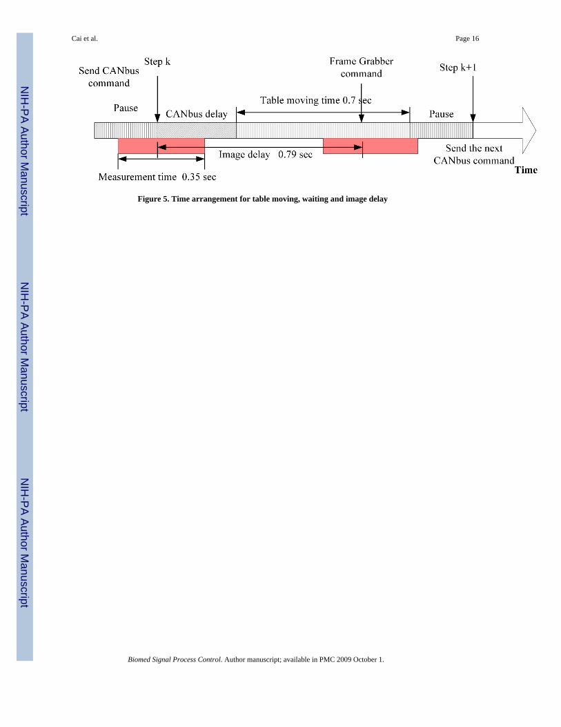
Figure 5. Time arrangement for table moving, waiting and image delay

Cai et al. Page 16

Biomed Signal Process Control. Author manuscript; available in PMC 2009 October 1.

NIH

-PA Author Manuscript

NIH

-PA Author Manuscript

NIH

-PA Author Manuscript

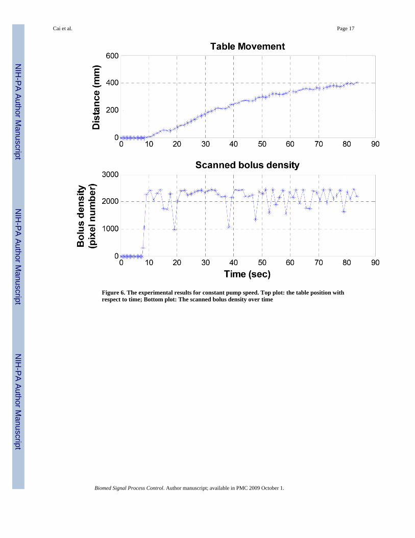
Figure 6. The experimental results for constant pump speed. Top plot: the table position withrespect to time; Bottom plot: The scanned bolus density over time

Cai et al. Page 17

Biomed Signal Process Control. Author manuscript; available in PMC 2009 October 1.

NIH

-PA Author Manuscript

NIH

-PA Author Manuscript

NIH

-PA Author Manuscript

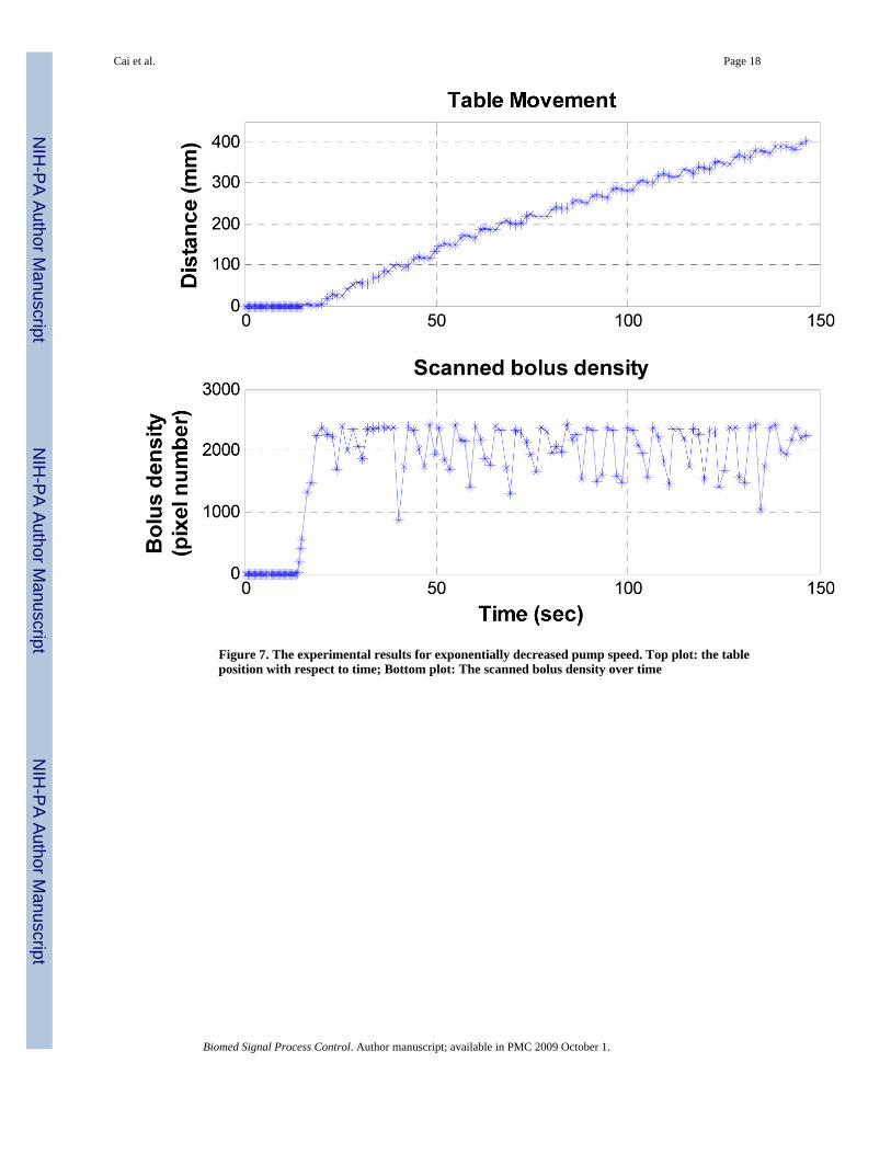
Figure 7. The experimental results for exponentially decreased pump speed. Top plot: the tableposition with respect to time; Bottom plot: The scanned bolus density over time

Cai et al. Page 18

Biomed Signal Process Control. Author manuscript; available in PMC 2009 October 1.

NIH

-PA Author Manuscript

NIH

-PA Author Manuscript

NIH

-PA Author Manuscript

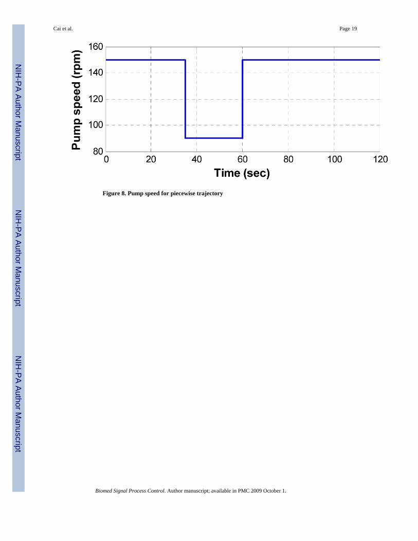
Figure 8. Pump speed for piecewise trajectory

Cai et al. Page 19

Biomed Signal Process Control. Author manuscript; available in PMC 2009 October 1.

NIH

-PA Author Manuscript

NIH

-PA Author Manuscript

NIH

-PA Author Manuscript

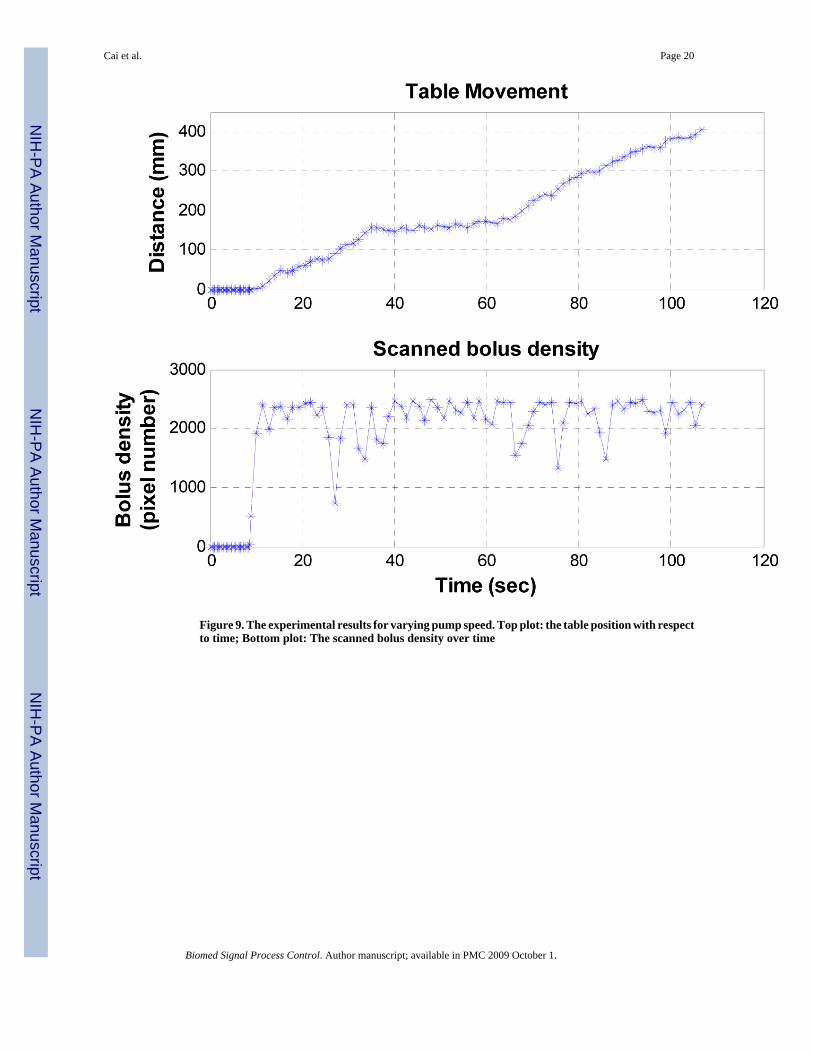
Figure 9. The experimental results for varying pump speed. Top plot: the table position with respectto time; Bottom plot: The scanned bolus density over time

Cai et al. Page 20

Biomed Signal Process Control. Author manuscript; available in PMC 2009 October 1.

NIH

-PA Author Manuscript

NIH

-PA Author Manuscript

NIH

-PA Author Manuscript

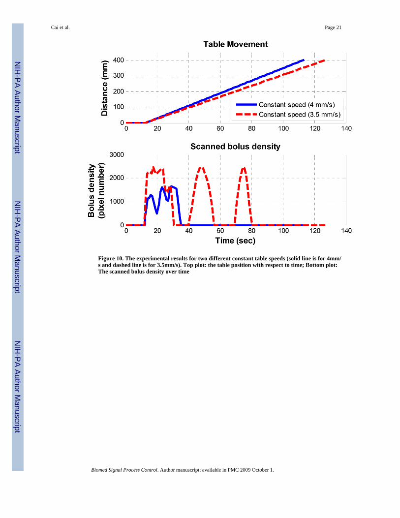
Figure 10. The experimental results for two different constant table speeds (solid line is for 4mm/s and dashed line is for 3.5mm/s). Top plot: the table position with respect to time; Bottom plot:The scanned bolus density over time

Cai et al. Page 21

Biomed Signal Process Control. Author manuscript; available in PMC 2009 October 1.

NIH

-PA Author Manuscript

NIH

-PA Author Manuscript

NIH

-PA Author Manuscript

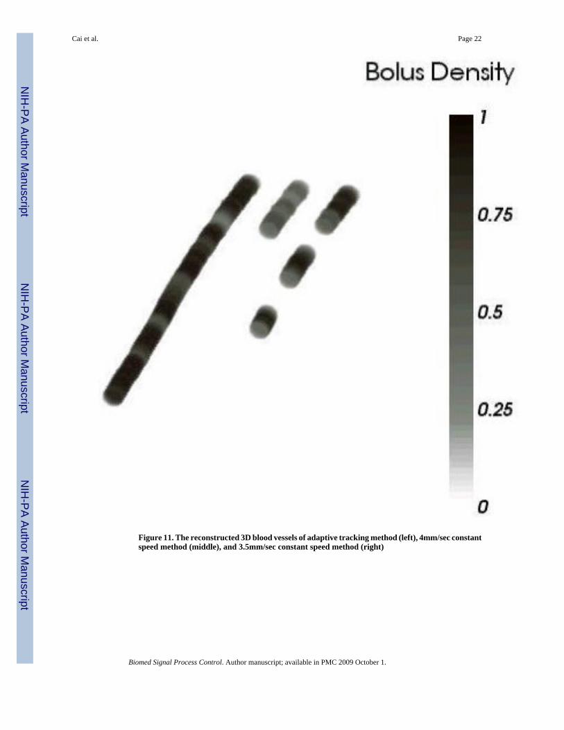
Figure 11. The reconstructed 3D blood vessels of adaptive tracking method (left), 4mm/sec constantspeed method (middle), and 3.5mm/sec constant speed method (right)

Cai et al. Page 22

Biomed Signal Process Control. Author manuscript; available in PMC 2009 October 1.

NIH

-PA Author Manuscript

NIH

-PA Author Manuscript

NIH

-PA Author Manuscript

NIH

-PA Author Manuscript

NIH

-PA Author Manuscript

NIH

-PA Author Manuscript

Cai et al. Page 23

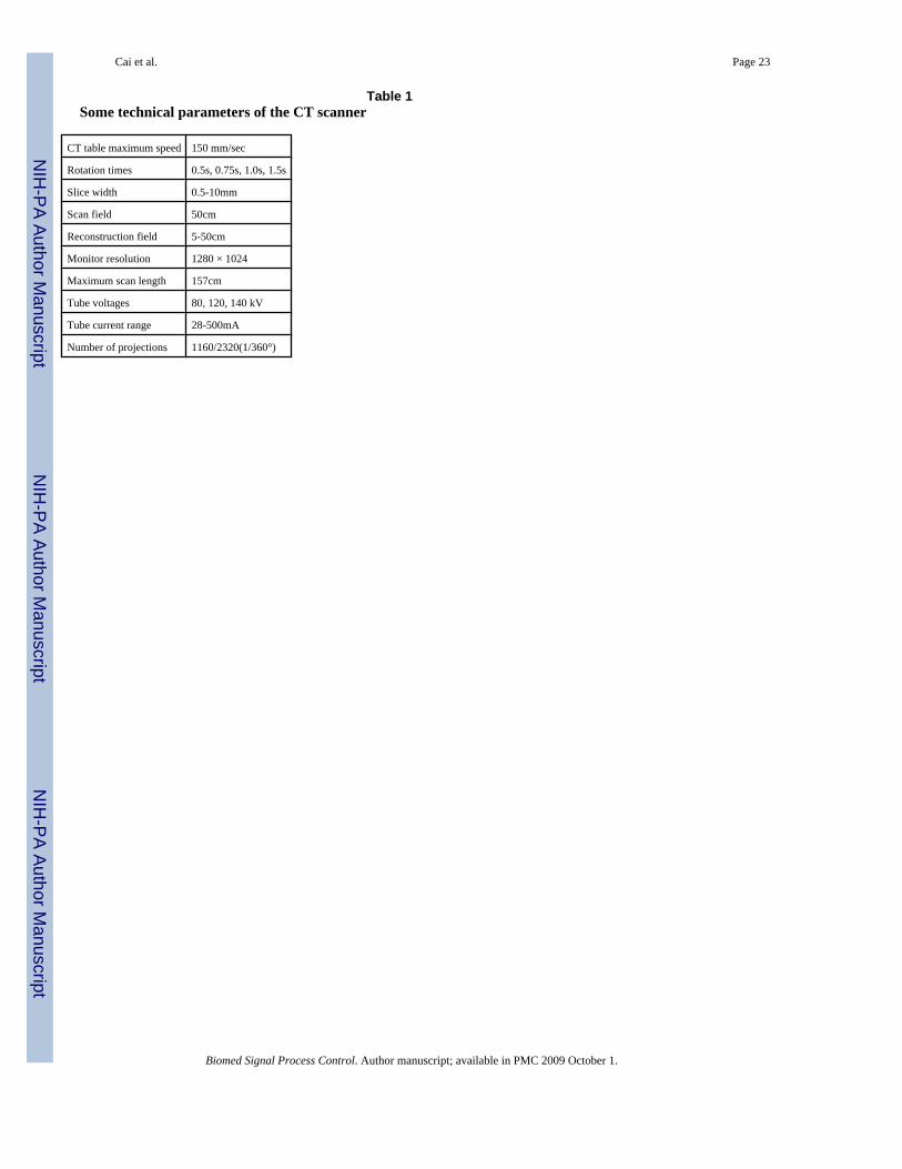
Table 1Some technical parameters of the CT scanner

CT table maximum speed 150 mm/sec

Rotation times 0.5s, 0.75s, 1.0s, 1.5s

Slice width 0.5-10mm

Scan field 50cm

Reconstruction field 5-50cm

Monitor resolution 1280 × 1024

Maximum scan length 157cm

Tube voltages 80, 120, 140 kV

Tube current range 28-500mA

Number of projections 1160/2320(1/360°)

Biomed Signal Process Control. Author manuscript; available in PMC 2009 October 1.

NIH

-PA Author Manuscript

NIH

-PA Author Manuscript

NIH

-PA Author Manuscript

Cai et al. Page 24

Table 2The scanning and control parameters

Scanning parameters

Slice Width: 1.0, collimation: 0.5mm

Voltage 120 kV

Current 81mA

Window 500 HU

Center 1500 HU

FOV (Field of View) 100mm

Center X -50mm

Center Y -60mm

Control parameters

Threshold to start the CT table 500

Alpha α 0.25

Variance threshold 200

Delay step l 1

Prescribed length 400 mm

Biomed Signal Process Control. Author manuscript; available in PMC 2009 October 1.

NIH

-PA Author Manuscript

NIH

-PA Author Manuscript

NIH

-PA Author Manuscript

Cai et al. Page 25

Table 3The averaged scanned density of the adaptive tracking method and the constant speed methods

Method Adaptive tracking method 4mm/s constant method 3.5mm/s constant method

Average scanned density 2212 260 772

Percentage of the maximum density 88.5% 10.4% 30.9%

Biomed Signal Process Control. Author manuscript; available in PMC 2009 October 1.