IEEE TRANSACTIONS ON BIOMEDICAL ENGINEERING, VOL. 59, NO. 7, JULY 2012 2019

Precise Segmentation of 3-D MagneticResonance Angiography

Ayman El-Baz*, Member, IEEE, Ahmed Elnakib, Member, IEEE, Fahmi Khalifa, Member, IEEE,Mohamed Abou El-Ghar, Patrick McClure, Ahmed Soliman, Member, IEEE, and Georgy Gimel’farb

Abstract—Accurate automatic extraction of a 3-D cerebrovas-cular system from images obtained by time-of-flight (TOF) orphase contrast (PC) magnetic resonance angiography (MRA) isa challenging segmentation problem due to the small size objectsof interest (blood vessels) in each 2-D MRA slice and complexsurrounding anatomical structures (e.g., fat, bones, or gray andwhite brain matter). We show that due to the multimodal natureof MRA data, blood vessels can be accurately separated from thebackground in each slice using a voxel-wise classification based onprecisely identified probability models of voxel intensities. To iden-tify the models, an empirical marginal probability distribution ofintensities is closely approximated with a linear combination of dis-crete Gaussians (LCDG) with alternate signs, using our previousEM-based techniques for precise linear combination of Gaussian-approximation adapted to deal with the LCDGs. The high accu-racy of the proposed approach is experimentally validated on 85real MRA datasets (50 TOF and 35 PC) as well as on syntheticMRA data for special 3-D geometrical phantoms of known shapes.

Index Terms—Cerebrovascular system, linear combination ofdiscrete Gaussians (LCDG), magnetic resonance angiography(MRA), segmentation.

I. INTRODUCTION

ACCURATE 3-D cerebrovascular system segmentationfrom magnetic resonance angiography (MRA) images

is one of the most important problems in practical computer-assisted medical diagnostics. Phase contrast (PC)-MRA pro-vides good suppression of background signals and quanti-fies blood flow velocity vectors for each voxel. Time-of-flight(TOF)-MRA is less quantitative, but it is fast and provides im-ages with high contrast. The most popular techniques for ex-tracting blood vessels from MRA data are scale-space filtering,

Manuscript received December 9, 2011; revised March 8, 2012 and April2, 2012; accepted April 10, 2012. Date of publication April 25, 2012; date ofcurrent version June 20, 2012. Asterisk indicates corresponding author.

*A. El-Baz is with the BioImaging Laboratory, Bioengineering De-partment, University of Louisville, Louisville, KY 40292 USA (e-mail:aselba01@louisville.edu).

A. Elnakib, F. Khalifa, P. McClure, and A. Soliman are with the BioImag-ing Laboratory, Bioengineering Department, University of Louisville,Louisville, KY 40292 USA (e-mail: aaelna02@louisville.edu; fahmi.khalifa@louisville.edu; psmccl01@louisville.edu; ahmed.soliman@louisville.edu).

M. A. El-Ghar is with the Radiology Department, Urology and NephrologyCenter, University of Mansoura, Mansoura 35516, Egypt (e-mail: maboel-ghar@yahoo.com).

G. Gimel’farb is with the Department of Computer Science,University of Auckland, Auckland 1142, New Zealand (e-mail:g.gimelfarb@auckland.ac.nz).

Color versions of one or more of the figures in this paper are available onlineat http://ieeexplore.ieee.org.

Digital Object Identifier 10.1109/TBME.2012.2196434

centerline-based methods, deformable models, statistical mod-els, and hybrid methods.

Multiscale filtering enhances curvilinear structures in 3-Dmedical images by convolving an image with Gaussian filtersat multiple scales [1]–[4]. Eigenvalues of the Hessian at eachvoxel are analyzed to determine the local shapes of 3-D struc-tures (by the eigenvalues, voxels from a linear structure, like ablood vessel, differ from those for a planar structure, specklenoise, or unstructured components). The multiscale filter outputforms a new enhanced image such that the curvilinear struc-tures become brighter whereas other components (e.g., specklenoise and planar structures such as skin) become darker [1].Such an image can be directly visualized, thresholded, or seg-mented using a deformable model. Alternatively, the obtainedeigenvalues define a candidate set of voxels corresponding to thecenterlines of the vessels [2]. Multiscale filter responses at eachof the candidates determine the likelihood that a voxel belongsto a vessel of each particular diameter. The maximal responseover all the diameters (scales) is assigned to each voxel, and asurface model of the entire vascular structure is reconstructedfrom the estimated centerlines and diameters. After segmentingthe filtered MRA image using thresholding, anisotropic diffu-sion techniques are used to remove noise, but preserve smallvessels [3]. Lacoste et al. [4] proposed a multiscale techniquebased on the Markov marked point processes to extract coronaryarteries from 2-D X-ray angiograms. Coronary vessels are mod-eled locally as piece-wise linear segments of varying locations,lengths, widths, and orientations. The vessels’ centerlines areextracted using a Markov object process specified by a uniformPoisson process. Process optimization was achieved via simu-lated annealing using a reversible Markov chain Monto Carloalgorithm.

Centerline minimal path-based techniques [5]–[7] formulatethe two-point centerline extraction as the minimum cost in-tegrated along the centerline path. Gulsun and Tek [5] usedmultiscale medialness filters to compute the cost of graph edgesin a graph-based minimal path detection method to extract thevessels’ centerlines. A post processing step, based on the lengthand scale of vessel centerlines, was performed to extract thefull vessel centerline tree. Pechaud et al. [6] presented an auto-matic framework to extract tubular structures from 2-D imagesby the use of shortest paths. Their framework combined mul-tiscale and orientation optimization to propagate 4-D (space +scale + orientation) paths on the 2-D images. Li and Yezzi [7]represented the 3-D vessel surface as a 4-D curve, with an addi-tional nonspatial dimension that described the radius (thickness)of the vessel. They applied a minimal path approach to find the

0018-9294/$31.00 © 2012 IEEE

2020 IEEE TRANSACTIONS ON BIOMEDICAL ENGINEERING, VOL. 59, NO. 7, JULY 2012

minimum path between user defined end points in the 4-D space.The detected path simultaneously described the vessel center-line as well as its surface. To overcome the possible shortcutproblem of minimal path techniques (i.e., track a false straightshortcut path instead of following the true curved path of thevessel), Zhu and Chung [8] used a minimum average-cost pathmodel to segment the 3-D coronary arteries from CT images.In their approach, the average edge cost is minimized alongpaths in the discrete 4-D graph constructed by image voxels andassociated radii.

Deformable model approaches to 3-D vascular segmentationattempt to approximate the boundary surface of the blood ves-sels [9]–[14]. An initial boundary, called a snake [15], evolvesin order to optimize a surface energy that depends on image gra-dients and surface smoothness. To increase the capture range ofthe evolving boundary, Xu and Prince [16] used a gradient vec-tor flow (GVF) field as an additional force to drive snakes intoobject concavities, which was latter used to segment the bloodvessels from 3-D MRA [9]. Geodesic active contours [17] im-plemented with level set techniques offer flexible topologicaladaptability to segment the MRA images [10] including moreefficient adaptation to local geometric structures represented.Fast segmentation of blood vessel surfaces is obtained by inflat-ing a 3-D balloon with fast marching methods [11].

Holtzman-Gazit et al. [12] extracted blood vessels in CTAimages based on variational principles. Their framework com-bined the Chan–Vese minimal variance model with a geometricedge alignment measure and the geodesic active surface model.Manniesing et al. [13] proposed a level set-based vascular seg-mentation method for finding vessel boundaries in CTA images.The level set function is attracted to the vessel boundaries basedon a dual object (vessels) and background intensity distribu-tions, which are estimated from the intensity histogram. Re-cently, Forkert et al. [14] used a vesselness filter to guide thedirection of a level set to extract vessels from TOF-MRA data.Compared to scale-space filtering, deformable models producemuch better experimental results, but have a common drawback,namely, a manual initialization. Also, both group approaches areslow when compared to statistical approaches.

Statistical extraction of a vascular tree is completely auto-matic, but its accuracy depends on the underlying probabil-ity models. The MRA images are multimodal in that the sig-nals (intensities, or gray levels) in each region of interest (e.g.,blood vessels, brain tissues, etc.) are associated with a particulardominant mode of the total marginal probability distribution ofsignals. To the best of our knowledge, adaptive statistical ap-proaches for extracting blood vessels from the MRA imageshave been proposed so far only by Wilson and Noble [18]for the TOF-MRA data and Chung and Noble [19] for thePC-MRA data. The former approach represents the marginaldata distribution with a mixture of two Gaussians and one uni-form component for the stationary cerebrospinal fluid (CSF),brain tissues, and arteries, respectively, whereas the latter ap-proach replaces the Gaussians with the more adequate Riciandistributions. To identify the mixture (i.e., estimate all its pa-rameters) a conventional EM algorithm is used in both cases. Itwas called a “modified EM” in [18], after replacing gray levels

in individual pixels considered by their initial EM scheme witha marginal gray level distribution. Actually, such a modificationsimply returns to what has been in common use for decadesfor density estimation (see e.g., [20]), while the individual pix-els appeared in their initial scheme only as an unduly verbatimreplica of a general EM framework.

Different hybrid approaches have attempted to combine theaforementioned approaches. For instance, a region-based de-formable contour for segmenting tubular structures is derivedin [21] by combining signal statistics and shape information.Law and Chung [22] guided a deformable surface model withthe second order intensity statistics and surface geometry tosegment blood vessels from TOF- and PC-MRA images. Acombination of a Gaussian statistical model with the maximumintensity projection (MIP) images acquired at three orthogonaldirections [23] allows for extracting blood vessels iterativelyfrom images acquired by rotational angiography. Alternatively,Hu and Hoffman [24] extracted the object boundaries by com-bining an iterative thresholding approach with region growingand component label analysis.

Mille et al. [25] used a generalized cylinder (GC) region-based deformable model for the segmentation of the angiogram.The GC is modeled as a central planar curve, acting as a me-dial axis, and a variable thickness. The GC is deformed bycoupling the evolution of the curve and thickness using narrowband energy minimization. This energy was transformed andderived in order to allow implementation on a polygonal linedeformed with gradient descent. Tyrrell et al. [26] proposed asuperelliposoid geometric model to extract the vessel bound-aries from in vivo optical slice data. Their approach predictedthe direction of the centerline utilizing a statistical estimator.Chen and Metaxas [27] combined a prior Gibbs random fieldmodel, marching cubes, and deformable models. First, the Gibbsmodel is used to estimate object boundaries using region infor-mation from 2-D slices. Then, the estimated boundaries and themarching cubes technique are used to construct a 3-D meshspecifying the initial geometry of a deformable model. Finally,the deformable model fits the data under the 3-D image gradientforces.

Recently, Shang et al. [28] developed an active contour frame-work to segment coronary artery and lung vessel trees from CTimages. A region, competition-based active contour model isused to segment thick vessels based on a Gaussian mixturemodel of the gray-level distribution of the vessel region. Then,a multiscale vector field, derived from the Hessian matrix ofthe image intensity, is used to guide the active contour throughthin vessels. Finally, the surface of the vessel is smoothed usinga vesselness function that selects between a minimal principalcurvature and a mean curvature criterion. Gao et al. [29] useda statistical model to find the main cerebrovascular structurefrom TOF-MRA. Then, an edge-strength function that incorpo-rates statistical region distribution and gradient information isused to guide a 3-D geometric deformable model to deal withthe undersegmentation. Dufour et al. [30] proposed an inter-active segmentation method that incorporates component-treesand example-based segmentation to extract the cerebrovasculartree from TOF-MRA data. Liao et al. [31] used a parametric

EL-BAZ et al.: PRECISE SEGMENTATION OF 3-D MAGNETIC RESONANCE ANGIOGRAPHY 2021

intensity model to extract thick and most thin vessels from 7-TMRA images. To fill the remaining gaps, a generative Markovrandom field method was applied.

The aforementioned overview shows the following limita-tions of the existing approaches.

1) Most of them presume only a single image type (e.g.,TOF- or PC-MRA).

2) Most of them require user interaction to initialize a vesselof interest.

3) Some deformable models assume circular vessel crosssections; this holds for healthy people, but not for patientswith a stenosis or an aneurysm.

4) All but statistical approaches are computationallyexpensive.

5) Known statistical approaches use only predefined proba-bility models that cannot fit all the cases because actualintensity distributions for blood vessels depend on the pa-tient, scanner, and scanning parameters.

Below we show the fast and highly accurate statistical ap-proach to extract blood vessels obtained when the probabilitymodels of each region of interest in TOF- or PC-MRA imagesare precisely identified rather than predefined as in [18] and [19].In our approach, the empirical gray level distribution for eachMRA slice is closely approximated with an LCDG. Then, thelatter is split into three individual LCDGs, one per region of in-terest. These regions are associated with three dominant modes:darker bones and fat, gray brain tissues, and bright blood ves-sels, respectively. The identified models specify an intensitythreshold for extracting blood vessels in that slice. Finally, a3-D connectivity filter is applied to the extracted voxels to se-lect the desired vascular tree. As our experiments show, moreprecise region models result in significantly better segmentationaccuracy compared to other methods.

II. SLICE-WISE SEGMENTATION WITH THE LCDG MODELS

We use the expected log-likelihood as a model identifica-tion criterion. Let X = (Xs : s = 1, . . . , S) denote a 3-D MRAimage containing S coregistered 2-D slices Xs = (Xs(i, j):(i, j) ∈ R;Xs(i, j) ∈ Q). Here, R and Q = {0, 1, . . . , Q − 1}are a rectangular arithmetic lattice supporting the 3-D imageand a finite set of Q-ary intensities (gray levels), respectively.Let Fs = (fs(q): q ∈ Q;

∑q∈Q fs(q) = 1, where q denotes the

gray level, be an empirical marginal probability distribution ofgray levels for the MRA slice Xs .

In accordance with [32], each such slice is considered asa K-modal image with a known number K of the dominantmodes related to the regions of interest (in our particular case,K = 3). To segment the slice by separating the modes, we haveto estimate the individual probability distributions of the signalsassociated with each mode fromFs . In contrast to a conventionalmixture of Gaussians, one per region [20], or slightly moreflexible mixtures involving other simple distributions, one perregion, as e.g., in [18] and [19], we closely approximate Fs

with LCDG. Then, the LCDG of the image is partitioned intosubmodels related to each dominant mode.

The discrete Gaussian (DG) is defined as the probability dis-tribution Ψθ = (ψ(q|θ): q ∈ Q) on Q of gray levels such thateach probability ψ(q|θ) relates to the cumulative Gaussian prob-ability function Φθ (q) as follows (here, θ is a shorthand notationθ = (μ, σ2) for the mean, μ, and variance, σ2):

ψ(q|θ) =

⎧⎪⎨

⎪⎩

Φθ (0.5) for q = 0

Φθ (q + 0.5) − Φθ (q − 0.5) for q = 1, . . . , Q−2

1 − Φθ (Q − 1.5) for q = Q − 1

The LCDG with Cp positive and Cn negative components suchthat Cp ≥ K

pw ,Θ (q) =Cp∑

r=1

wp,rψ(q|θp,r ) −Cn∑

l=1

wn,lψ(q|θn,l) (1)

has obvious restrictions on its weights w = [wp,. , wn,. ], namely,all the weights are nonnegative and

Cp∑

r=1

wp,r −Cn∑

l=1

wn,l = 1. (2)

Generally, the true probabilities are nonnegative: pw ,Θ (q) ≥ 0for all q ∈ Q. Therefore, the probability distributions compriseonly a proper subset of all the LCDGs in (1), which may havenegative components pw ,Θ (q) < 0 for some q ∈ Q.

Our goal is to find a K-modal probability model thatclosely approximates the unknown marginal gray level distri-bution. Given Fs , its Bayesian estimate F is as follows [20]:f(q) = (|R|fs(q) + 1)/(|R| + Q), and the desired model hasto maximize the expected log-likelihood of the statistically in-dependent empirical data by the model parameters:

L(w,Θ) =∑

q∈Q

f(q) log pw ,Θ (q). (3)

For simplicity, we do not restrict the identification procedureto only the true probability distributions, but instead checkthe validity of the restrictions during the procedure itself. TheBayesian probability estimate F with no zero or unit values in(3) ensures that a sufficiently large vicinity of each componentf(q) complies to the restrictions.

To precisely identify the LCDG-model including the numbersof its positive and negative components, we adapt to the LCDGsour EM-based techniques [32] for identification of a probabil-ity density with a continuous linear combination of Gaussian-model. For completeness, the adapted algorithms are outlinedin Appendix A.

The entire segmentation algorithm is as follows.1) For each successive MRA slice Xs , s = 1, . . . , S,

a) Collect the marginal empirical probability distribu-tion Fs = (fs(q): q ∈ Q) of gray levels.

b) Find an initial LCDG-model that closely approx-imates Fs by using the initializing algorithm inAppendix A to estimate the numbers Cp − K, Cn ,and parameters w, Θ (weights, means, and vari-ances) of the positive and negative DGs.

2022 IEEE TRANSACTIONS ON BIOMEDICAL ENGINEERING, VOL. 59, NO. 7, JULY 2012

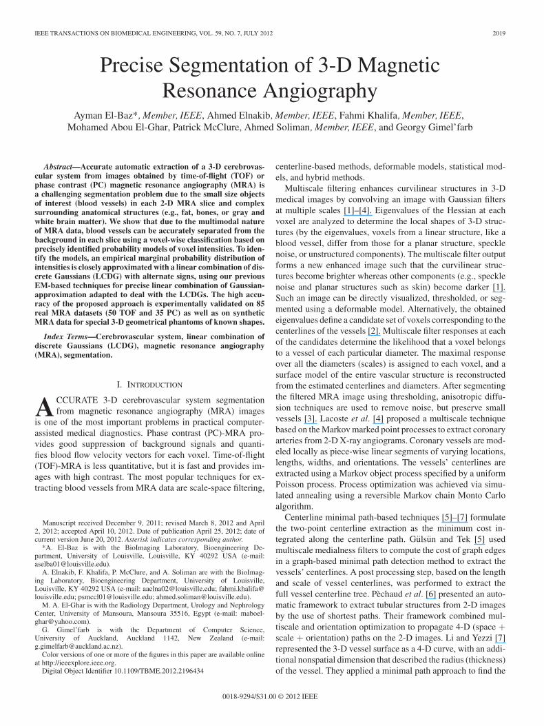
Fig. 1. 2-D schematic illustration of measuring segmentation errors betweenthe ground truth G and proposed automatic segmentation C.

c) Refine the LCDG-model with the fixed Cp and Cn

by adjusting all other parameters with the modifiedEM algorithm in Appendix B.

d) Split the final LCDG-model into K submodels,one per each dominant mode, by minimizing theexpected errors of misclassification and select theLCDG-submodel with the largest mean value (i.e.,the submodel corresponding to the brightest pixels)as the model of the desired blood vessels.

e) Extract the blood vessels’ voxels in this MRAslice using the intensity threshold t separating theirLCDG-submodel from the background ones.

2) Eliminate artifacts from the whole set of the extractedvoxels using a connectivity filter that selects the largestconnected tree structure built by a 3-D volume growingalgorithm [33].1

The main goal of the whole procedure is to find the thresholdfor each MRA slice that extracts the brighter blood vessels fromtheir darker background in such a way that the vessels’ bound-aries are accurately separated from the surrounding structuresthat may have similar brightness along these boundaries. Theinitialization at Step 1b produces the LCDG with the nonnega-tive starting probabilities pw ,Θ (q). While the refinement at Step1c increases the likelihood, the probabilities continue to be non-negative. In our experiments presented as follows, the oppositesituations have never been met.

III. SEGMENTATION ACCURACY

The proposed segmentation is evaluated based on calculatingthe percentage of the total error (false positive and false nega-tive) with respect to the “ground truth.” For the evaluation, wemeasured true positive (TP), true negative (TN), false positive(FP), and false negative (FN) segmentations (see Fig. 1). LetC, G, and R denote the segmented region, its “ground truth”counterpart, and the whole image lattice, respectively. Then,TP = |C ∩ G|; FP = |C − C ∩ G|; FN = |G − C ∩ G|; andTN = |R − C ∪ G|. The total error is defined in line with [34]as: ε = FN+FP

TP+FN = FN+FPG .

1Step 2 is necessary due to MRA sensitivity to tissues with short T1 responses(e.g., subcutaneous fat) that may obscure the blood vessels in the segmentedvolume.

(a)

(b)

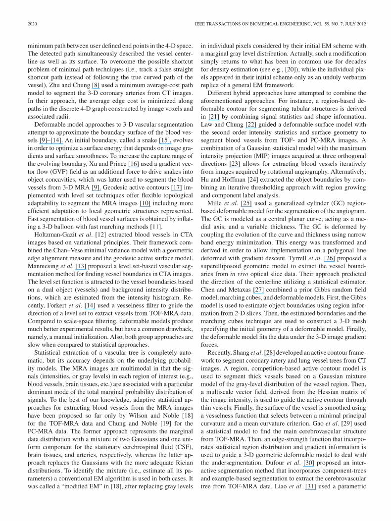
Fig. 2. Typical (a) TOF-MRA and (b) PC-MRA slices with the domi-nant Gaussian mixtures P3 = (p3 (q) : q ∈ Q) laid over the distributionsF = (f (q) : q ∈ Q).

IV. EXPERIMENTAL RESULTS

Experiments in extracting blood vessels have been conductedon 50 3-D TOF-MRA and 35 PC-MRA datasets, acquired withthe Picker 1.5-T Edge MRI scanner with the following spatialresolution and size:

Resolution, mm Size, voxelsTOF-MRA 0.43 × 0.43 × 1.0 512 × 512 × 93PC-MRA 0.86 × 0.86 × 1.0 256 × 256 × 123

Both the image types are three-modal (K = 3) with the afore-mentioned signal classes of dark gray bones and fat, gray braintissues, and light gray blood vessels. Typical 2-D TOF- andPC-MRA slices and their three-class dominant Gaussian mix-tures P3 approximating the estimated marginal distributions Fare shown in Fig. 2.

A. Segmentation of Natural TOF- and PC-MRA Images

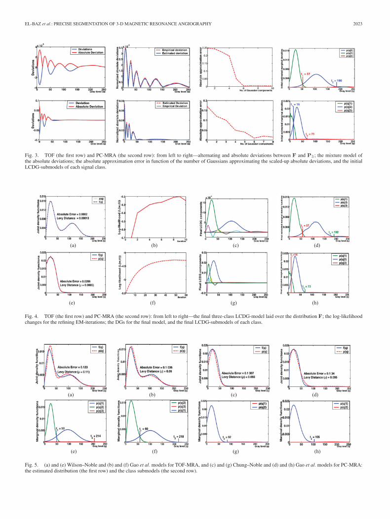
Fig. 3 illustrates how Step 1b of our algorithm builds an initialLCDG model for the TOF- and PC-MRA images in Fig. 2.Absolute deviations |f(q) − p3(q)| are scaled up to make theunit sums of the positive or absolute negative deviations for q =0, . . . , Q − 1. The minimum approximation errors are obtainedin both the cases with the six-component Gaussian mixtures.Each initial LCDG model can be split, if necessary, into thethree LCDG-submodels for each signal class.

Fig. 4 presents the final LCDG-models after Step 1c of ouralgorithm and shows successive changes of the log-likelihoodduring the refining EM-process. For the TOF- and PC-MRAimages, the first nine EM-iterations increase the log-likelihoodfrom −5.7 to −5.2 and −5.5 to −4.4, respectively. The finalLCDG-submodels of each class (Step 1d) suggest that thresholdst2 = 192 and t2 = 73 separate blood vessels from the TOF-and PC-MRA images, respectively, with the minimum expectedmisclassification error.

To highlight advantages of our approach, Fig. 5 shows theapproximation of the distributions F for the TOF- and PC-MRAimages in Fig. 2 with the three-component Wilson–Noble [18],

EL-BAZ et al.: PRECISE SEGMENTATION OF 3-D MAGNETIC RESONANCE ANGIOGRAPHY 2023

Fig. 3. TOF (the first row) and PC-MRA (the second row): from left to right—alternating and absolute deviations between F and P3 ; the mixture model ofthe absolute deviations; the absolute approximation error in function of the number of Gaussians approximating the scaled-up absolute deviations, and the initialLCDG-submodels of each signal class.

(a) (b) (c) (d)

(e) (f) (g) (h)

Fig. 4. TOF (the first row) and PC-MRA (the second row): from left to right—the final three-class LCDG-model laid over the distribution F; the log-likelihoodchanges for the refining EM-iterations; the DGs for the final model, and the final LCDG-submodels of each class.

(e) (f) (g) (h)

(a) (b) (c) (d)

Fig. 5. (a) and (e) Wilson–Noble and (b) and (f) Gao et al. models for TOF-MRA, and (c) and (g) Chung–Noble and (d) and (h) Gao et al. models for PC-MRA:the estimated distribution (the first row) and the class submodels (the second row).

2024 IEEE TRANSACTIONS ON BIOMEDICAL ENGINEERING, VOL. 59, NO. 7, JULY 2012

t2 = 192 t2 = 214 t2 = 218

t2 = 187 t2 = 209 t2 = 198

t2 = 168 t2 = 185 t2 = 201(a) (b) (c) (d) (e) (f)

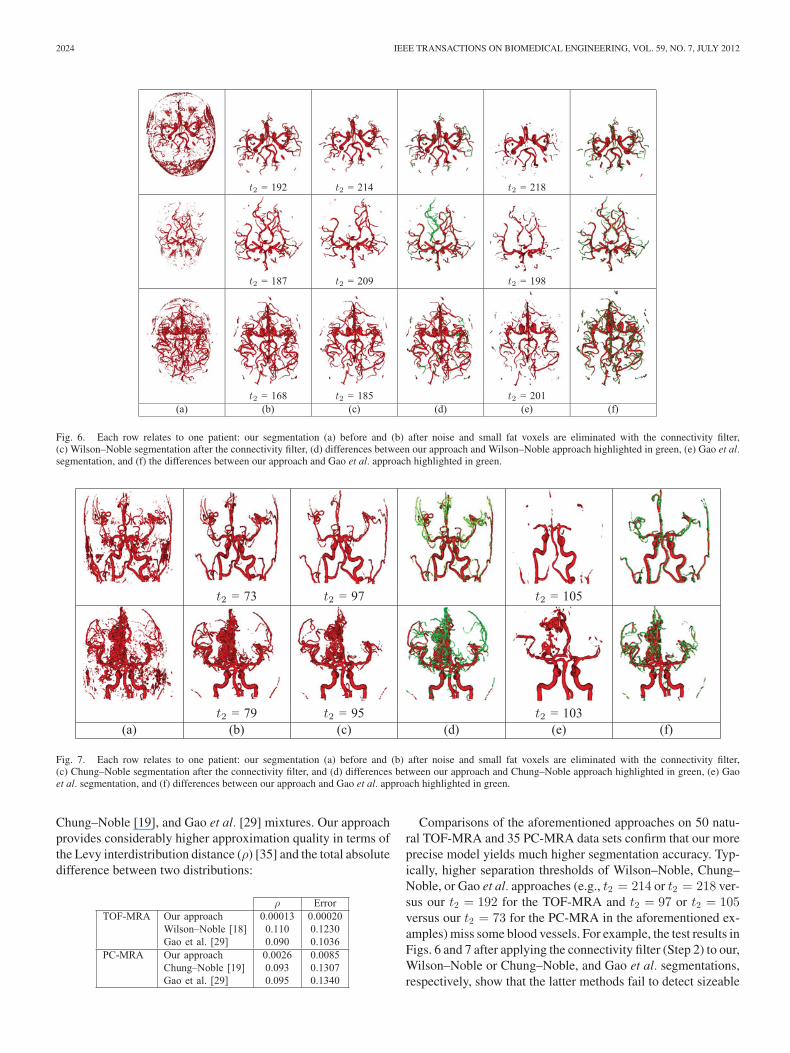
Fig. 6. Each row relates to one patient: our segmentation (a) before and (b) after noise and small fat voxels are eliminated with the connectivity filter,(c) Wilson–Noble segmentation after the connectivity filter, (d) differences between our approach and Wilson–Noble approach highlighted in green, (e) Gao et al.segmentation, and (f) the differences between our approach and Gao et al. approach highlighted in green.

t2 = 73 t2 = 97 t2 = 105

t2 = 79 t2 = 95 t2 = 103(a) (b) (c) (d) (e) (f)

Fig. 7. Each row relates to one patient: our segmentation (a) before and (b) after noise and small fat voxels are eliminated with the connectivity filter,(c) Chung–Noble segmentation after the connectivity filter, and (d) differences between our approach and Chung–Noble approach highlighted in green, (e) Gaoet al. segmentation, and (f) differences between our approach and Gao et al. approach highlighted in green.

Chung–Noble [19], and Gao et al. [29] mixtures. Our approachprovides considerably higher approximation quality in terms ofthe Levy interdistribution distance (ρ) [35] and the total absolutedifference between two distributions:

ρ ErrorTOF-MRA Our approach 0.00013 0.00020

Wilson–Noble [18] 0.110 0.1230Gao et al. [29] 0.090 0.1036

PC-MRA Our approach 0.0026 0.0085Chung–Noble [19] 0.093 0.1307Gao et al. [29] 0.095 0.1340

Comparisons of the aforementioned approaches on 50 natu-ral TOF-MRA and 35 PC-MRA data sets confirm that our moreprecise model yields much higher segmentation accuracy. Typ-ically, higher separation thresholds of Wilson–Noble, Chung–Noble, or Gao et al. approaches (e.g., t2 = 214 or t2 = 218 ver-sus our t2 = 192 for the TOF-MRA and t2 = 97 or t2 = 105versus our t2 = 73 for the PC-MRA in the aforementioned ex-amples) miss some blood vessels. For example, the test results inFigs. 6 and 7 after applying the connectivity filter (Step 2) to our,Wilson–Noble or Chung–Noble, and Gao et al. segmentations,respectively, show that the latter methods fail to detect sizeable

EL-BAZ et al.: PRECISE SEGMENTATION OF 3-D MAGNETIC RESONANCE ANGIOGRAPHY 2025

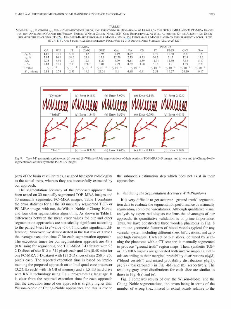
TABLE IMINIMUM εn , MAXIMUM εx , MEAN ε SEGMENTATION ERROR, AND THE STANDARD DEVIATION σ OF ERRORS ON THE 30 TOF-MRA AND 30 PC-MRA IMAGES

FOR OUR APPROACH (OA) AND THE WILSON–NOBLE (WN) OR CHUNG–NOBLE (CN) ONE, RESPECTIVELY, AS WELL AS FOR THE OTHER ALGORITHMS USING

ITERATIVE THRESHOLDING (IT) [24], GRADIENT-BASED DEFORMABLE MODEL (DMG) [15], DEFORMABLE MODEL BASED ON THE GRADIENT VECTOR FLOW

(GVF) [16], AND STATISTICAL SEGMENTATION FOLLOWED BY 3-D DEFORMABLE SURFACE (GAO et al. [29])

TOF-MRA PC-MRAOA WN IT DMG GVF Gao OA CN IT DMG GVF Gao

εn,% 1.05 0.17 5.71 11.5 3.95 0.19 0.07 1.01 4.72 10.60 2.37 1.23εx,% 3.95 14.6 34.3 23.9 15.1 12.79 2.33 9.75 30.2 21.5 12.9 13.3ε,% 0.73 6.91 17.1 12.1 6.29 8.79 0.41 3.59 11.01 11.50 3.53 5.17σ,% 0.83 6.10 7.03 2.99 3.01 5.79 0.52 3.80 5.13 1.9 1.99 2.77P-value ≤ 10−4 ≤ 10−4 ≤ 10−4 ≤ 10−4 ≤ 10−4 ≤ 10−4 ≤ 10−4 ≤ 10−4 ≤ 10−4 ≤ 10−4

T , minute 0.81 0.73 2.33 14.1 21.31 8.1 0.48 0.41 2.51 16.27 24.19 9.17

“Cylinder” (a) Error 0.18% (b) Error 3.97% (c) Error 0.14% (d) Error 2.12%

“Spiral” (a) Error 1.34% (b) Error 9.52% (c) Error 0.79% (d) Error 4.01%

“Tree” (a) Error 0.31% (b) Error 4.64% (c) Error 0.18% (d) Error 3.14%

Fig. 8. True 3-D geometrical phantoms: (a) our and (b) Wilson–Noble segmentations of their synthetic TOF-MRA 3-D images, and (c) our and (d) Chung–Noblesegmentations of their synthetic PC-MRA images.

parts of the brain vascular trees, assigned by expert radiologiststo the actual trees, whereas they are successfully extracted byour approach.

The segmentation accuracy of the proposed approach hasbeen tested on 30 manually segmented TOF–MRA images and30 manually segmented PC–MRA images. Table I combinesthe error statistics for all the 30 manually segmented TOF- orPC-MRA images with our, the Wilson–Noble or Chung–Noble,and four other segmentation algorithms. As shown in Table I,differences between the mean error values for our and othersegmentation approaches are statistically significant accordingto the paired t-test (a P-value < 0.05 indicates significant dif-ference). Moreover, we demonstrated in the last row of Table Ithe average execution time T for each segmentation approach.The execution times for our segmentation approach are 49 s(0.81 min) for segmenting one TOF-MRA 3-D dataset with 932-D slices of size 512 × 512 pixels each and 29 s (0.48 min) forone PC-MRA 3-D dataset with 123 2-D slices of size 256 × 256pixels each. The reported execution time is based on imple-menting the proposed approach on an Intel quad-core processor(3.2 GHz each) with 16 GB of memory and a 1.5 TB hard drivewith RAID technology using C++ programming language. Itis clear from the reported execution time for each approachthat the execution time of our approach is slightly higher thanWilson–Noble or Chung–Noble approaches and this is due to

the submodels estimation step which does not exist in theirapproaches.

B. Validating the Segmentation Accuracy With Phantoms

It is very difficult to get accurate “ground truth” segmenta-tion data to evaluate the segmentation performance by manuallysegmenting complete vasculatures. Although qualitative visualanalysis by expert radiologists confirms the advantages of ourapproach, its quantitative validation is of prime importance.Thus, we have constructed three wooden phantoms in Fig. 8to imitate geometric features of blood vessels typical for anyvascular system including different sizes, bifurcations, and zeroand high curvature. Each set of 2-D slices, obtained by scan-ning the phantoms with a CT scanner, is manually segmentedto produce “ground truth” region maps. Then, synthetic TOF-or PC-MRA signals are generated with inverse mapping meth-ods according to their marginal probability distributions p(q|3)(“blood vessels”) and mixed probability distributions p(q|1),p(q|2) (“background”) in Fig. 4(d) and (h), respectively. Theresulting gray level distributions for each slice are similar tothose in Fig. 4(a) and (e).

Fig. 8 compares results of our, the Wilson–Noble, and theChung–Noble segmentations, the errors being in terms of thenumber of wrong (i.e., missed or extra) voxels relative to the

2026 IEEE TRANSACTIONS ON BIOMEDICAL ENGINEERING, VOL. 59, NO. 7, JULY 2012

”eerT“”laripS“”rednilyC“

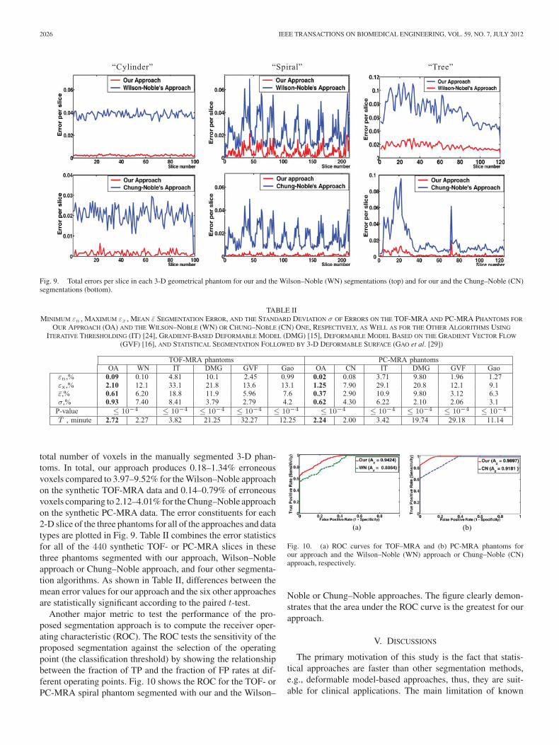
Fig. 9. Total errors per slice in each 3-D geometrical phantom for our and the Wilson–Noble (WN) segmentations (top) and for our and the Chung–Noble (CN)segmentations (bottom).

TABLE IIMINIMUM εn , MAXIMUM εx , MEAN ε SEGMENTATION ERROR, AND THE STANDARD DEVIATION σ OF ERRORS ON THE TOF-MRA AND PC-MRA PHANTOMS FOR

OUR APPROACH (OA) AND THE WILSON–NOBLE (WN) OR CHUNG–NOBLE (CN) ONE, RESPECTIVELY, AS WELL AS FOR THE OTHER ALGORITHMS USING

ITERATIVE THRESHOLDING (IT) [24], GRADIENT-BASED DEFORMABLE MODEL (DMG) [15], DEFORMABLE MODEL BASED ON THE GRADIENT VECTOR FLOW

(GVF) [16], AND STATISTICAL SEGMENTATION FOLLOWED BY 3-D DEFORMABLE SURFACE (GAO et al. [29])

TOF-MRA phantoms PC-MRA phantomsOA WN IT DMG GVF Gao OA CN IT DMG GVF Gao

εn,% 0.09 0.10 4.81 10.1 2.45 0.99 0.02 0.08 3.71 9.80 1.96 1.27εx,% 2.10 12.1 33.1 21.8 13.6 13.1 1.25 7.90 29.1 20.8 12.1 9.1ε,% 0.61 6.20 18.8 11.9 5.96 7.6 0.37 2.90 10.9 9.80 3.12 6.3σ,% 0.93 7.40 8.41 3.79 2.79 4.2 0.62 4.30 6.22 2.10 2.06 3.1P-value ≤ 10−4 ≤ 10−4 ≤ 10−4 ≤ 10−4 ≤ 10−4 ≤ 10−4 ≤ 10−4 ≤ 10−4 ≤ 10−4 ≤ 10−4

T , minute 2.72 2.27 3.82 21.25 32.27 12.25 2.24 2.00 3.42 19.74 29.18 11.14

total number of voxels in the manually segmented 3-D phan-toms. In total, our approach produces 0.18–1.34% erroneousvoxels compared to 3.97–9.52% for the Wilson–Noble approachon the synthetic TOF-MRA data and 0.14–0.79% of erroneousvoxels comparing to 2.12–4.01% for the Chung–Noble approachon the synthetic PC-MRA data. The error constituents for each2-D slice of the three phantoms for all of the approaches and datatypes are plotted in Fig. 9. Table II combines the error statisticsfor all of the 440 synthetic TOF- or PC-MRA slices in thesethree phantoms segmented with our approach, Wilson–Nobleapproach or Chung–Noble approach, and four other segmenta-tion algorithms. As shown in Table II, differences between themean error values for our approach and the six other approachesare statistically significant according to the paired t-test.

Another major metric to test the performance of the pro-posed segmentation approach is to compute the receiver oper-ating characteristic (ROC). The ROC tests the sensitivity of theproposed segmentation against the selection of the operatingpoint (the classification threshold) by showing the relationshipbetween the fraction of TP and the fraction of FP rates at dif-ferent operating points. Fig. 10 shows the ROC for the TOF- orPC-MRA spiral phantom segmented with our and the Wilson–

(a) (b)

Fig. 10. (a) ROC curves for TOF–MRA and (b) PC-MRA phantoms forour approach and the Wilson–Noble (WN) approach or Chung–Noble (CN)approach, respectively.

Noble or Chung–Noble approaches. The figure clearly demon-strates that the area under the ROC curve is the greatest for ourapproach.

V. DISCUSSIONS

The primary motivation of this study is the fact that statis-tical approaches are faster than other segmentation methods,e.g., deformable model-based approaches, thus, they are suit-able for clinical applications. The main limitation of known

EL-BAZ et al.: PRECISE SEGMENTATION OF 3-D MAGNETIC RESONANCE ANGIOGRAPHY 2027

statistical approaches is that they are based on predefined prob-ability models that cannot fit all possible cases due to the factthat actual intensity distributions for blood vessels depend onthe patient, scanner, and scanning parameters. In response tothis problem, we propose a fast and highly accurate adaptivestatistical approach to extract blood vessels from TOF- andPC-MRA images. In this approach, the probability models ofeach region of interest are precisely identified using an LCDG-based approximation, rather than predefined approximations asused in other statistical approaches [18], [19]. This makes theproposed approach suitable to work with any imaging modality,e.g., TOF- or PC-MRA images.

Comparisons between the proposed approach and the cur-rent state-of-the-art segmentation approaches on both real MRAdatasets (TOF and PC) and synthetic phantoms confirm thatour more precise model yields a much higher segmentation ac-curacy, as evidenced by the error analysis and statistical testsshown in Tables I and II. In addition, qualitative analysis inFig. 6 shows that other approaches fail to detect sizeable partsof the brain vascular trees, assigned by expert radiologists to theactual trees, whereas these sections are successfully extractedwhen using our approach. In terms of practicality of compu-tations, the execution time of our approach is faster than de-formable model-based approaches [15], [16], [29] and slightlyslower than current well-known statistical approaches [18], [19]due to the submodels estimation step which does not exist inthese approaches.

For the proposed LCDG probabilistic model, the only man-ually provided parameter is the number K of the dominantmodes in the empirical mixture (that is, the number of ob-jects to be separated by the segmentation). We have investi-gated a possibility to estimate this number by searching forthe global maximum of the conditional expected log-likelihoodL(K) =

∑q∈Q f(q)

∑Kk=1 π(k|q) log ψ(q|θk ) where π(k|q) is

the conditional probability of the kth component ψ(q|θk ) ofthe discrete Gaussian mixture having K dominant modes, giventhe gray level q. However, this approach meets with difficultieswhen adjacent dominant modes resembling a single expandedpeak need to be resolved, or when a dominant low-weightedmode need to be detected in the presence of higher-weightedmodes. We expect to overcome these difficulties in our futurework.

VI. CONCLUSION

This paper presents a generalized automated approach for theextraction of the 3-D cerebrovascular system that is suitablefor any imaging modality, e.g., CTA, TOF-MRA, and PC-MRAimages. Voxel intensity-based models for classification are em-ployed using a linear combination of discrete Gaussians (LCDG)to accurately identify the empirical distribution of the gray levelintensity in the images. A modified EM-based approach hasbeen used to identify the LCDG models. Accuracy and valid-ity of the method has been demonstrated on 85 in vivo MRAdatasets along with synthetic phantom data, confirming the highaccuracy and speed of the proposed LCDG-based extractionmethod.

APPENDIX

A. Sequential EM-Based Initialization

The initial LCDG model, closely approximating a givenmarginal gray level distribution F, is built using the conventionalEM-algorithm [20], [36] adapted to the DGs. The approximationinvolves the following steps.

1) The distribution F is approximated with a mixture PK ofK positive DGs relating each to a dominant mode.

2) Deviations between F and PK are approximated withthe alternating “subordinate” components of the LCDG asfollows.

a) The positive and the negative deviations are sepa-rated and scaled up to form two seemingly “proba-bility distributions” Dp and Dn .

b) The same conventional EM algorithm is used iter-atively to find a subordinate mixture of positive ornegative DGs that approximates best Dp or Dn ,respectively (i.e., the sizes Cp − K and Cn of themixtures are found by minimizing sequentially thetotal absolute error between each “distribution” Dp

or Dn and its mixture model by the number of thecomponents).

c) The obtained positive and negative subordinate mix-tures are scaled down and then added to the dominantmixture yielding the initial LCDG model of the sizeC = Cp + Cn .

The resulting initial LCDG has K dominant weightswp,1 , . . . , wp,K such that

∑Kr=1 wp,r = 1, and a number of sub-

ordinate weights of smaller values such that∑Cp

r=K +1 wp,r −∑Cn

l=1 wn,l = 0.

B. Modified EM Algorithm for Refining LCDGs

The initial LCDG is refined by approaching the local maxi-mum of the log-likelihood in (3) with the EM process adaptingthat in [32] to the DGs. The latter extends in turn the conventionalEM-process in [20] and [36] onto the alternating components.

Let p[m ]w ,Θ (q)=

∑Cp

r=1 w[m ]p,r ψ(q|θ[m ]

p,r ) −∑Cn

l=1 w[m ]n,l ψ(q|θ[m ]

n,l )denote the current LCDG at iteration m. Relative contributionsof each signal q ∈ Q to each positive and negative DG at itera-tion m are specified by the respective conditional weights

π[m ]p (r|q) =

w[m ]p,r ψ(q|θ[m ]

p,r )

p[m ]w ,Θ (q)

; π[m ]n (l|q) =

w[m ]n,l ψ(q|θ[m ]

n,l )

p[m ]w ,Θ (q)

(4)such that the following constraints hold:

Cp∑

r=1

π[m ]p (r|q) −

Cn∑

l=1

π[m ]n (l|q) = 1; q = 0, . . . , Q − 1. (5)

The following two steps iterate until the log-likelihood is in-creasing and its changes become small:

E-step[m ]: Find the weights of (4) under the fixed parametersw[m−1] , Θ[m−1] from the previous iteration m − 1, and

2028 IEEE TRANSACTIONS ON BIOMEDICAL ENGINEERING, VOL. 59, NO. 7, JULY 2012

M-step[m ]: Find conditional maximum likelihood estimates(MLEs) w[m ] , Θ[m ] by maximizing L(w,Θ) under thefixed weights of (4).

Considerations closely similar to those in [20] and [36] showthis process converges to a local log-likelihood maximum. Thefurther evidence in [32] demonstrates it is actually a block re-laxation minimization-maximization process (in a very generalway, this is also shown in [36]). Let the log-likelihood of (3) berewritten in the equivalent form with the constraints of (5) asunit factors:

L(w[m ],Θ[m ]) =Q∑

q=0

f(q)

[ Cp∑

r=1

π[m ]p (r|q) log p[m ](q)

−Cn∑

l=1

π[m ]n (l|q) log p[m ](q)

]

. (6)

Let the terms log p[m ](q) in the first and second bracketsbe replaced with the equal terms log w

[m ]p,r + log ψ(q|θ[m ]

p,r ) −log π

[m ]p (r|q) and log w

[m ]n,l + log ψ(q|θ[m ]

n,l ) − log π[m ]n (l|q), re-

spectively, which follow from (4). At the E-step, the con-ditional Lagrange maximization of the log-likelihood of (6)under the Q restrictions of (5) results just in the weightsπ

[m+1]p (r|q) and π

[m+1]n (l|q) of (4) for all r = 1, . . . , Cp ; l =

1, . . . , Cn and q ∈ Q. At the M-step, the DG weights w[m+1]p,r =

∑q∈Q f(q)π[m+1]

p (r|q) and w[m+1]n,l =

∑q∈Q f(q)π[m+1]

n (l|q)follow from the conditional Lagrange maximization of the log-likelihood in (6) under the restriction of (2) and the fixed condi-tional weights of (4). Under these latter, the conventional MLEsof the parameters of each DG stem from maximizing the log-likelihood after each difference of the cumulative Gaussians isreplaced with its close approximation with the Gaussian density(below “c” stands for “p” or “n,” respectively):

μ[m+1]c,r =

1

w[m+1]c,r

∑

q∈Q

q · f(q)π[m+1]c (r|q)

(σ[m+1]c,r )2 =

1

w[m+1]c,r

∑

q∈Q

(q − μ

[m+1]c,i

)2 · f(q)π[m+1]c (r|q).

This modified EM-algorithm is valid until the weights w arestrictly positive. The iterations should be terminated when thelog-likelihood of (3) almost does not change or begins to de-crease due to accumulation of rounding errors.

The final mixed LCDG-model pC (q) is partitioned into the KLCDG-submodels P[k ] = [p(q|k) : q ∈ Q], one per class k =1, . . . ,K, by associating the subordinate DGs with the dominantterms so that the misclassification rate is minimal.

REFERENCES

[1] Y. Sato, S. Nakajimaa, N. Shiragaa, H. Atsumia, S. Yoshidab, T. Kollerc,G. Gerigc, and R. Kikinisa, “Three-dimensional multi-scale line filterfor segmentation and visualization of curvilinear structures in medicalimages,” Med. Image Anal., vol. 2, no. 2, pp. 143–168, 1998.

[2] K. Krissian, G. Malandain, N. Ayache, R. Vaillant, and Y. Trousset, “Modelbased multiscale detection of 3D vessels,” in Proc. IEEE Conf. Comput.Vision Pattern Recognit., 1998, pp. 722–727.

[3] F. Catte, P-L. Lions, J.-M. Morel, and T. Coll, “Image selective smoothingand edge detection by nonlinear diffusion,” SIAM J. Numer. Anal., vol. 29,no. 1, pp. 182–193, 1992.

[4] C. Lacoste, G. Finet, and I. E. Magnin, “Coronary tree extraction fromX-ray angiograms using marked point processes,” in Proc. IEEE Int. Symp.Biomed. Imag., 2006, pp. 157–160.

[5] M. A. Gulsun and H. Tek, “Robust vessel tree modeling,” in Proc. Int.Conf. Med. Image Comput. Comput—Assist. Intervent., 2008, pp. 602–611.

[6] M. Pechaud, R. Keriven, and G. Peyre, “Extraction of tubular structuresover an orientation domain,” in Proc. IEEE Conf. Comput. Vis. PatternRecognit., 2009, pp. 336–342.

[7] H. Li and A. Yezzi, “Vessels as 4-D curves: Global minimal 4-D paths toextract 3-D tabular surfaces and centerlines,” IEEE Trans. Med. Imag.,vol. 26, no. 9, pp. 1213–1223, Sep. 2007.

[8] N. Zhu and A. C. Chung, “Minimum average-cost path for real time 3Dcoronary artery segmentation of CT images,” in Proc. Int. Conf. Med.Image Comput. Comput.—Assist. Intervent., 2011, pp. 436–444.

[9] A. C. Jalba, M. H. Wilkinson, and J. B. Roerdink, “CPM: A deformablemodel for shape recovery and segmentation based on charged particles,”IEEE Trans. Pattern Anal. Mach. Intell., vol. 26, no. 10, pp. 1320–1335,Oct. 2004.

[10] L. M. Lorigo, O. D. Faugeras, W. E. Grimson, R. Keriven, R. Kikinis,A. Nabavi, and C. F. Westin, “Curves: Curve evolution for vessel segmen-tation,” Med. Image Anal., vol. 5, no. 3, pp. 195–206, 2001.

[11] T. Deschamps and L. D. Cohen, “Fast extraction of tubular and tree 3D sur-faces with front propoagation methods,” in Proc. IEEE Int. Conf. PatternRecognit., 2002, pp. 731–734.

[12] M. Holtzman-Gazit, R. Kimmel, N. Peled, and D. Goldsher, “Segmenta-tion of thin structures in volumetric medial images,” IEEE Trans. Image.Process., vol. 15, no. 3, pp. 354–363, Feb. 2006.

[13] R. Manniesing, B. K. Velthuis, M. S. van Leeuwen, I. C. van der Schaaf,P. J. van Laar, and W. J. Niessen, “Level set based cerebral vasculature seg-mentation and diameter quantification in CT angiography,” Med. Image.Anal., vol. 10, no. 2, pp. 200–214, 2006.

[14] N. D. Forkert, D. Saring, T. Illies, J. Fiehler, J. Ehrhardt, H. Handels,and A. Schmidt-Richberg, “Direction-dependent level set segmentationof cerebrovascular structures,” Proc. SPIE, Image Process.: Med. Imag.,vol. 7962, pp. 1–8, 2011.

[15] M. Kass, A. Witkin, and D. Terzopoulos, “Snakes: Active contour models,”Int. J. Comput. Vision, vol. 1, pp. 321–331, 1988.

[16] C. Xu and J. L. Prince, “Snakes, shapes, and gradient vector flow,” IEEETrans. Image Process., vol. 7, no. 3, pp. 359–369, 1998.

[17] V. Caselles, R. Kimmel, and G. Sapiro, “Geodesic active contours,” Int.J. Comput. Vision, vol. 22, no. 1, pp. 61–79, 1997.

[18] D. L. Wilson and J. A. Noble, “An adaptive segmentation algorithm fortime-of-flight MRA data,” IEEE Trans. Med. Imag., vol. 18, no. 10,pp. 938–945, Oct. 1999.

[19] A. C. S. Chung and J. A. Noble,“Statistical 3D vessel segmentation usinga Rician distribution,” in Proc. Int. Conf. Med. Image Comput. Comput.—Assist. Intervent., 1999, pp. 82–89.

[20] A. Webb, Statistical Pattern Recognition. New York: Wiley, 2002.[21] D. Nain, A. Yezzi, and G. Turk, “Vessels segmentation using a shape

driven flow,” in Proc. Int. Conf. Med. Image Comput. Comput.—Assist.Intervent., 2004, pp. 51–59.

[22] M. W. Law and A. C. Chung, “A deformable surface model for vascularsegmentation,” in Proc. Int. Conf. Med. Image Comput. Comput.—Assist.Intervent., 2009, pp. 59–67.

[23] R. Gan, A. C. Chung, C. K. Wong, and S. C. Yu, “Vascular segmentationin three-dimensional rotational angiography based on maximum intensityprojections,” in Proc. IEEE Int. Symp. Biomed. Imag., 2004, pp. 133–136.

[24] S. Hu and E. A. Hoffman, “Automatic lung segmentation for accuratequantization of volumetric X-ray CT images,” IEEE Trans. Med. Imag.,vol. 20, no. 6, pp. 490–498, Jun. 2001.

[25] J. Mille, R. Bone, and L. D. Cohen, “Region-based 2D deformable gen-eralized cylinder for narrow structures segmentation,” in Proc. Eur. Conf.Comput. Vision, 2008, pp. 392–404.

[26] J. Tyrrell, E. di Tomaso, D. Fuja, R. Tong, K. Kozak, R. K. Jain, andB. Roysam, “Robust 3-D modeling of vascuature imagery using superel-lipsoids,” IEEE Trans. Med. Imag., vol. 26, no. 2, pp. 223–237, Feb.2007.

[27] T. Chen and D. N. Metaxas, “Gibbs prior models, marching cubes, anddeformable models: A hybrid framework for 3D medical image segmenta-tion,” in Proc. Int. Conf. Med. Image Comput. Comput.—Assist. Intervent.,2003, pp. 703–710.

EL-BAZ et al.: PRECISE SEGMENTATION OF 3-D MAGNETIC RESONANCE ANGIOGRAPHY 2029

[28] Y. Shang, R. Deklerck, E. Nyssen, A. Markova, J. de Mey, X. Yang, andK. Sun, “Vascular active contour for vessel tree segmentation,” IEEETrans. Biomed. Eng., vol. 58, no. 4, pp. 1023–1032, Apr. 2011.

[29] X. Gao, Y. Uchiyama, X. Zhou, T. Hara, T. Asano, and H. Fujita, “A fastand fully automatic method for cerebrovascular segmentation on time-of-flight (TOF) MRA image,” J. Digital Imag., vol. 24, no. 4, pp. 609–625,2011.

[30] A. Dufour, N. Passat, B. Naegel, and J. Baruthio, “Interactive 3D brainvessel segmentation from an example,” in Proc. IEEE Int. Symp. Biomed.Imag., 2011, pp. 1121–1124.

[31] W. Liao, K. Rohr, C.-K. Kang, Z.-H. Cho, and S. Worz, “A generativeMRF approach for automatic 3D segmentation of cerebral vasculaturefrom 7 Tesla MRA images,” in Proc. IEEE Int. Symp. Biomed. Imag.,2011, pp. 2041–2044.

[32] G. Gimel’farb, A. A. Farag, and A. El-Baz, “Expectation-maximizationfor a linear combination of Gaussians,” in Proc. IEEE Int. Conf. PatternRecognit., 2004, vol. 3, pp. 422–425.

[33] M. Sabry, C. B. Sites, A. A. Farag, S. Hushek, and T. Moriaty, “A fastautomatic method for 3D volume segmentation of the human cerebrovas-cular,” in Proc. Comput.—Assist. Radiol. Surg., 2002, pp. 382–387.

[34] K. Suzuki, “Computerized segmentation of organs by means of geodesicactive-contour level-set algorithm,” in Multi Modality State-of-the-ArtMedical Image Segmentation and Registration Methodologies, vol. 1,A. El-Baz, R. Acharya, M. Mirmedhdi, and J. Suri, eds., New York:Springer-Verlag, 2011, ch. 4, pp. 103–128.

[35] J. W. Lamperti, Probability. New York: Wiley, 1996.[36] T. Hastie, R. Tibshirani, and J. Friedman, The Elements of Statistical

Learning. New York: Springer-Verlag, 2001.

Author’ photographs and biographies not available at the time of publication.