CHAPTER 1

INTRODUCTION

CHAPTER 1 INTRODUCTION

Financial Management has long been recognized as an important tool in construction management. However,

the construction industry suffers the largest rate of insolvency of any sector of the economy. Many construction

companies fail because of poor financial management, especially inadequate attention to cash flow forecasting

.The major problem that construction managers encounter in making financial decisions involves both the

uncertainty and ambiguity surrounding expected cash flows. Cash flows are essential to solvency. They can be

presented as a record of something that has happened in the past, such as the sale of a particular product, or

forecasted into the future, representing what a business or a person expects to take in and to spend. Cash flow is

crucial to an entity's survival. Having ample cash on hand will ensure that creditors, employees and others can

be paid on time. If a business or person does not have enough cash to support its operations, it is said to be

insolvent, and a likely candidate for bankruptcy should the insolvency continue.

In the case of complex projects, the problem of uncertainty and ambiguity assumed even greater proportion

because of the difficulty in predicting the impact of unexpected changes on construction progress and

consequently, on cash flows. The uncertainty and ambiguity are caused not only by project-related problems but

also by the economic and technological factors.

1.1Problem Statement:

The serious importance of the cash-flow prediction for construction contractors it has been indicated. A reliable

cash flow prediction can help to accurately identify the expected project financial requirements. So that, decision

can be made at a suitable time regarding the potential sources of this finance. Unfortunately, construction project

cash-flow is mainly affected by many uncertain but predictable factors. Among these are accidents, thefts,

inflation rate, weather inclement, changes interest rate, strikes …… etc.

Through the literature survey, it was noticed that the majority cash-flow prediction models have been based on

standard deterministic cash flow S-Curves, developed using the traditional manual approach, mathematical and

statistical models. Many of these models failed to consider and analyses the risk factors such as changes in the

design or specifications, contract conditions pertaining to cash in flow, interim valuations and certificates and

construction programming issues such as inclement weather responsible for the considerable variations in the

1

CHAPTER 1

INTRODUCTION

modeled cash flow profiles. Hence, it is safe to say that a reliable cash-flow prediction should take into

consideration the effect of these risk factors. Consequently it is expected that a probabilistic rather than a

deterministic cash flow model can best typify the stochastic nature of the cash flow prediction.

1.2 Study objective and Scope

The objective of this study is twofold. First, is to identify the most important risk factors affecting the cash

flow prediction of construction projects in Egypt. Second, is the development of a probabilistic cash flow

prediction model that can take into consideration the serious effect of those risk factors. The scope of this

study will be only confined to building construction projects.

1.3 Study Methodology:

The study conducted through the following sequence:

1. A literature review have been carried out to cover the most important studies in this research area.

2. Based on this literature review, a questionnaire survey was conducted to identify the most important

risk factors affecting cash-flow prediction.

3. The development of a probabilistic cash flow model was also considered.

4. The validity of the proposed model have been tested based on a selected case study application.

1.4 Thesis Outline

This section outlines the various chapters of the thesis. After this introducing chapter, Chapter 2 presents

literature review. Such review presents the different methods used to maintain the cash flow profiles. It also

identifies the different risk factors that should be involved in the cash flow forecasting. Chapter 3 presents

the questionnaire design and the data collection process. The main goal of this survey is to identify the main risk

factors affecting the cash flow modeling. Chapter 4 discusses the development of the proposed probabilistic

cash flow prediction model. Chapter 5 illustrates testing the validity of the proposed cash-flow model. Finally,

Chapter 6 summarize the study and its major conclusions and recommendations.

2

CHAPTER 2

LITERATURE REVIEW

CHAPTER 2

LITERATURE REVIEW 2.1 Introduction

This chapter presents a brief description of the previously developed cash flow prediction methods,

attention will be also given to the effect of the budget with different scenarios of project schedule & budget,

identifying the risk factors involved in cash flow forecasting. So, two axis are available to work on , the first

one is the identifying of the main risk factors that affect the modeling of the cash flow forecasting models,

the second is the implementation of these risk factors into a net cash flow model to maintain a realistic cash

flow profile that can adequately consider these risk factors.

A proactive approach to project cash flow management relies heavily on the use of a forecasting model that

is, on the other hand, capable of generating reasonably accurate forecasts and, on the other hand, offers the

flexibility which enables the financial manager to challenge the outcome of the forecast in the direction of

corporate financial objectives of the organization.

The traditional approach to cash flow prediction usually involves the breakdown of the bill of quantities in

line with the contract programmer to produce an estimated expenditure profile. This could be expected to be

reasonably precise provided that the bill of quantities is accurate and the contract program is complied with

(Lowe, 1987). However, is likely to be slow and costly to produce; as such, several attempts have been made

to devise a ‘short cut’ method of estimation, which will be both quicker and cheaper to utilize. Attempts

have been made at the mathematical formulae and statistical based modeling of construction cash flow in

both the contractor and client’s organizations. This was demonstrated by the development of a series of

typical S-curves by many researchers (Kaka and Price, 1993). The models obtained by these researchers rest

on the assumption that reasonably accurate prediction is possible by means of a single formula utilizing two

or more parameters which may vary according to the type, nature, location, value and duration of the contract.

The main issue that all previous researches focused on maintaining a cash flow model or net cash flow model

to help the contractor on the planning phase and a few of them on the construction phase. The problem that

all these researches ignore the risks that affect the construction process and do not implement any risk factors

in the estimation of the cash flow which cause a non-reliable cash flow forecasting and so a more cash

problem to the contractor that makes him incapable to carry out his financial obligations.

The importance of carefully managing cash flow can hardly be overstated. It “cuts to the heart of the financial

viability of a construction company” (Kenley, 2003) and leads to long-term profitability or bankruptcy from

an inability to pay financing fees, debt reduction, and operations from inflows.

3

CHAPTER 2

LITERATURE REVIEW

(Lowe, 1987) argued that the main factors responsible for variation in project cash flow could be grouped

under five main headings of contractual, programming, pricing, valuation and economic factors. (Harris and

Mccaffer, 1995) identified the factors that affect capital lock-up which ultimately affect project cash flow

profile to include the margin (profit margin or contribution), retention, claims, tender unbalancing, delay in

receiving payments from clients and delay in paying labours, plant hirers, materials suppliers and

subcontractors. (Calvert, 1986) identified other factors to include seasonal effects on construction works,

variability in preliminary expenses, contract extensions of time for inclement weather and valuation of

variations. (Kaka, A.P. and Price, A.D.F, 1993) in developing a model for cash flow forecasting identified

other risk factors affecting cash flow profiles to include estimating error, tendering strategies, cost and

duration variances. The identified risk factors have been reported to affect cash flow profiles as well as

significantly impacting on the modeling of cash flow. However the perception of the contractors to the

likelihood of the risk factors occurring in different project types and of varying scope and duration is yet to

be investigated.

2.2 Net Cash Flow Models

The most essential terms used are described as follows (Odeyinka, H A and Lowe, J G, 2001)

Cash flow is essentially the movement of money into and out of your business; it's the cycle of cash inflows

and cash outflows that determine your business' solvency.

Cash flow = Receipts – Disbursements

Cash flow analysis is the study of the cycle of your business' cash inflows and outflows, with the purpose of

maintaining an adequate cash flow for your business, and to provide the basis for cash flow management.

Net cash flow is the balance between the cash out flow and the cash in flow

Net Cash flow = Positive cash flow (receipts) - Negative cash flow (disbursements)

In an early work (Nazem, 1968) proposed a net cash flow model based on historic data, with the aim of

discovering standard balance curves. He attempted to develop an 'ideal net cash flow reference curve' for use

in predicting future capital requirements. Contractors do not undertake only one project at a time; therefore

4

CHAPTER 2

LITERATURE REVIEW

Nazem emphasized the overall requirements of the firm, not the individual position for a project. He argued

that an overlay of all projects would yield the capital requirements for a company over time. Nazem's

proposal required that the ideal reference curve be derived as an average of a reasonable sample of projects.

This method has not been successfully followed up, possibly due to problems in deriving such an average;

however, there is evidence that some firms employ a similar technique as part of their management systems.

2.2.1 Ideal Curves and Previous Models

In the absence of an ideal net cash flow curve, previous researchers have used ideal value curves to produce

net cash flow profiles. The method defines the cash-in curve as the value curve minus any retention held,

with an allowance for time lag. Similarly, the cost curve is derived from the earnings curve using specified

lags and percentages of earnings.

The possibility of building an ideal value curve based on historic data has been the subject of a considerable

amount of research (Bromilow and Henderson, 1977); (Singh and Woon, 1984); (Drak, 1987); (Hudson,

1978). Although these approaches have gained general acceptance, they have not been without criticism.

(Hardy, 1970) Found that there was no close correlation between the figures given for 25 projects considered,

even when the projects were similar.

(Oliver, 1984) Analysed projects collected from three construction companies. He concluded that,

although the number of projects analysed was statistically small, construction projects are individually

unique and follow such diverse routes that value curves based on historical data are not capable of providing

the accuracy required for individual contract control.

These and other curves were used in computer packages to forecast the net cash flow for construction

projects. (Ashley and Teicholz, 1977)Developed a model based on the value curve to assist in the analysis

of cash flow over the life of a project. The model also calculates the cost of borrowing and the present value

of a given cash flow. (Mackay, 1971)Developed a computer program that estimated the shape of the value

curve defined by a series of up to 20 break points connected by a series of straight lines. From this model,

various cost categories with their associated time delays, contract value, profit, retentions, etc., were input

to compute the resultant cash flow throughout the project. Through test simulations of the program, he

determined that the shape made little difference in the cash flow pattern. This approach has been adopted in

commercial software packages for use by quantity surveyors and contractors. However, a library of typical

S-curves is installed to allow the user to select an S-curve that closely represents his project. In addition, the

user may input his own estimated curve if a suitable one cannot be found in the library.

5

CHAPTER 2

LITERATURE REVIEW

Other researchers thought that value curves were unique to single contracts, and therefore should be

estimated for each project. (Peterman, 1972) Developed a net cash flow model using value curves based on

bar charts of bill items. (Allsop, 1980) Linked a cash flow model to an estimating program which already

existed at Loughborough University of Technology. The program used the estimated cost and estimated

value with the contract schedules to calculate the cash flow of the project. The preparation of work schedules

involves complex and expensive analyses at a time when resources are least available, and therefore the use

of such models should be strongly justified. The justification lies in the importance of cash flow forecasts at

the tendering stage and the level of inaccuracy of simplified S-curve models.

Studies on the accuracy of models based on ideal value curves are in conflict. The feasibility of building

ideal value curves for different project types is questionable. There is evidence that single curves cannot be

fitted accurately through even one type of project. Mackay's sensitivity analysis of net cash flow profiles to

different value curves implies that either net cash flow curves conform to predictable patterns or they are

sensitive to the selection of systematic delays.

(Kenley, 1986) Studied the variability of net cash flow profiles by collecting the cash-out and cash-in data

from 26 commercial and industrial projects. The goodness of fit was reasonably accurate and 26 net cash

flow profiles were produced. Comparisons between the results indicated that there was a wide degree of

variation between the profiles of individual projects.

2.2.2 Weighted Mean Delays Method

From another point of view, some researches have concentrated on the method of 'weighted mean delays'

in order to develop a method for modelling individual construction project net cash flows. This method

involves applying systematic delays to a cash inflow profile, in order to reckon the outflow profile. The

balance between the two is the net cash flow.

(Peterman, 1972) Proposed an early model utilizing standard delays, and this was followed by (Ashley and

Teicholz, 1977) and (Mccaffer, 1979). McCaffer refined the approach using forecast income schedules based

on network analysis. These models did not use standard sigmoid (S) curves as their base, although both

(Ashley and Teicholz, 1977)and (Mccaffer, 1979)suggested that standard curves may adequately replace the

more complex and expensive derivation of project income schedules.

(Hardy, 1970) Utilized a system with gross cash flow curves derived from the application of built-up rates

to a network schedule (PERT analysis). He used this, together with an outgoings curve (inferred through

applied systematic delays), to derive the net cash flow forecast for a project.

Hardy's model would be difficult to test because of the shortage of available cash payment data. This

shortage made it difficult to test the model against historical data; thus the delay system was initiated. Hardy

6

CHAPTER 2

LITERATURE REVIEW

was able to perform some testing on hypothetical projects, obtaining an indication of the model's ability to

be consistent and accommodate change, but not of its accuracy. The model is therefore largely intuitive,

based on the results of estimated (and assumed constant) delays which could not be tested using empirical

data.

(Mackay, 1971) Used standard curves for the originating curves rather than curves derived from forecast

work schedules. Subsequently McCaffer produced a comprehensive computer program which forecast

construction project net cash flows using standard curves. Use was made of standard curves because the

preparation of work schedules (which were only as accurate as the schedule) involved complex and

expensive analyses at a time when resources would be least available.

The systematic delay method used by (Mccaffer, 1979) and reported by (Tucker and Rahilly, 1982), relied

on the hypothesis that the value curve can be modelled by the use of standard curves, and that the cash-in

curve and cash-out curve can be modelled by the application of delay factors to the value curve. The value

curve represents the certified value of the work, so the delay of payment from the client (due to contractual

or other causes) gives the cash-in curve. The outflow or cost curve is equivalent to the value curve for

outgoings, and represents the value of work done (as compared to that certified) and is calculated from the

value curve through applied factors. The cash-out curve is then found from the cost curve, as the outlay will

usually occur after a period of delay which varies according to the outlay and project conditions. McCaffer

used a method of weighted mean delays to derive the component curves from the standard value set at the

commencement of this procedure.

McCaffer's procedure is similar to that used by Ashley and Teicholz who defined the cash-in curve as the

earnings minus held retention, with allowance for lag. Similarly, the cost curve was derived from the earnings

curve using specified lags and percentages of earnings.

The results of the weighted mean delay method have not been directly compared with the actual historical

data for a project forecast. This is unfortunate because one observation by (Mackay, 1971)was that the

selection of an appropriate originating (standard) curve did not greatly affect the net cash flow model yielded.

This suggests that the accuracy of systematic delay models is dependent solely upon the selection of

appropriate delays, and not upon the selection of the originating curve. It may seem inherently more likely

that net cash flow would be more affected by the period between expenditure and income rather than the rate

of progress of the project, this approach ignores the possibility that the components may have differing rates

of progress (curve slopes) - and thus the weighted mean delay method would be insufficient to derive one

component curve from the other. A comparison with real data may have indicated that differing component

curve slopes yield widely different net cash flow curves in practice, as was found within the present project.

Both the ideal reference curve and weighted mean delay models have limitations, one being that they use

methods which yield consistent results regardless of the selection of originating curves. There is a large

7

CHAPTER 2

LITERATURE REVIEW

degree of variability between individual project net cash flows; therefore it is necessary to develop a model

capable of adjusting to a wide range of variable profiles. Such a model is unlikely to use polynomial

regression of net cash flow data, as 'the regression analysis has failed to produce a convincing explanation

of cash flow differences' ( (O'Keefe, 1971), cited in Kerr, 1973). Hence further research must return to the

work of (Jepson, 1969) who suggested that 'generating' or 'component' curves (the inflow and outflow

profiles) be used to derive individual project net cash flows.

(Peterman, 1972) Illustrated the large variation possible between the net cash flows for various projects, and

the derivation of the residual or working capital profile from component income and cost ogives. Similarly

(Nazem, 1968), (Mccaffer, 1979)and (Neo, 1978) illustrated the interaction between the component ogives

and the residual.

2.2.3 Idiographic Method vs. Nomothetic Method

Several approaches to the analysis have been used and they may all be characterized as nomothetic. They

attempted to discover general laws and principles across categorized or non-categorized groups of

construction projects, with the purpose of a-priori prediction of cash flows. In contrast an idiographic

methodology; the search for specific laws pertaining to individual projects.

The idiographic-nomothetic debate flourished within the social sciences, from the 1950s through to the early

1960s (Runyan, 1983). The contention arose, according to (De Groot, 1969), from the inability to classify

the social sciences as either cultural or natural sciences. The social sciences, to which construction

management must belong, have components of both cultural sciences (for example history) and natural

sciences (for example physics), and have aspects which are 'individual and unique; they are own - (character)

- describing: idiographic' (De Groot, 1969). De Groot claimed that 'if one seeks to conduct a scientific

investigation into an individual, unique phenomenon. The regular methodology of (natural) science provides

no help'. As construction projects are unique it would seem logical that their cash flows should be considered

as individual and unique.

The nomothetic approach assumes there are consistent similarities between projects hen produce what are

viewed as non-transient industry averages for groups of projects. This rationale ignores idiosyncratic

differences between projects, discounting their significance by treating such variation as random (hence

implying unimportant) error. While Idiographic method recognizes that variation between projects is a

product of their individuality rather than a random error about an established ideal.

Individual variation between projects is caused by a multiplicity of factors, the great majority of which can

neither be isolated in sample data, nor predicted in future projects. Some existing cash flow models hold that

generally two factors, date and project type, are sufficient to derive an ideal construction project cash flow

curve. Such convenient divisions ignore the complex interaction between such influences as economic and

8

CHAPTER 2

LITERATURE REVIEW

political climate, managerial structure and actions, union relations and personality conflicts. Many of these

factors have been perceived to be important in related studies such as cost, time and quality performance of

building projects (Ireland, 1983), and therefore models which ignore all these factors in cash flow research

must be questioned.

The majority of previous studies use historical data. Standard curve models, based on historic data, have

been extensively used in cash flow research[or example: (Balkau, 1975); (Bromilow, 1978); (Bromilow, and

Henderson, 1977); (Drak, 1987); (Hudson, 1978); (Hudson and Maunick, 1974); (Kerr, 1973); (Mccaffer,

1979); (Singh and Woon, 1984); (Tucker and Rahilly, 1982)] Although these approaches have gained general

acceptance, they have not been without criticism. (Hardy, 1970) Found that there was no close similarity

between the ogives for 25 projects considered, even when the projects were within one category. This

implicit support for an idiographic methodology was subsequently ignored, despite the problems which some

researchers found in supporting their models. Hudson observed that 'difficulties are to be expected when

trying to apply a simple mathematical equation to a real life situation, particularly one as complex as the

erection of a building' [(Hudson and Maunick, 1974); (Hudson, 1978)]. It is interesting to contrast the size

of Hardy's sample of 25 projects, with the relatively small samples used by many of the researchers finding

nomothetic, ideal curves. For example (Bromilow and Henderson, 1977) used four projects, while (Hardy,

1970) used three projects and (Peer, 1982) used four projects.

There has been an implied trend over time towards an idiographic construction project cash flow model. The

early models, which may be termed 'industry' models, searched for generally applicable patterns across the

entire industry. When it was recognized that this was unlikely to be achieved, greater flexibility was

introduced by searching for patterns within groups or categories of project (the division usually being made

according to project type and/or dollar value - e.g. (Hudson, and Maunick, 1974). This still wholly

nomothetic approach was modified by (Berny and Howes, 1982) who adapted the (Hudson and Maunick,

1974) category model to a form which could reflect the specific form of individual projects. Even within

categories, it had been found that there were occasional projects which did not fit the forecast expenditure

well (Hudson and Maunick, 1974); (Hudson, 1978).

(Berny and Howes, 1982) Designed methods for calculating the specific curve for a given project, based on

their general equation. In doing so they pointed the way for future research in this field. Their model made

a very important cognitive step. By proposing an equation for the general case of an individual project curve,

as distinct from the curve of the general (standard) function, it moved from a nomothetic to an idiographic

approach.

9

CHAPTER 2

LITERATURE REVIEW

(Kenley and Wilson, 1986) take Consideration of the idiographic-nomothetic debate led to that the natural

science methodology was inappropriate for unique phenomena such as construction projects due to a

multiplicity of factors and influences effect project cash flows, many of which are unquantifiable and have

differential impact.

It is therefore contended that an idiographic methodology is more appropriate to the study of construction

project cash flows, than is a nomothetic methodology, and a nomothetic methodology can only be supported

if a significant similarity can be shown to exist within groups. The experimental hypothesis is that there is

substantial variation between projects.

In Their models it was noticed that the projects examined have yielded individual profiles, which support

Hardy's (1970) contention that no close similarities exist between projects. It is their belief that group models

are both functionally as well as conceptually in error.

2.2.4 Probabilistic Cost and Duration Estimating

As with all variability in activity cost and duration due to expected and unexpected changes upon the

project various phases, Probabilistic estimation is needed. Recently, commercial computer programs have

been developed with the specific purpose of probabilistic estimating [e.g. Monte Carlo simulation (Monte

Carloe Version 2.0.) and @RISK for Project (2012)]. These simulation applications are capable of

developing integrated probabilistic cost and duration estimating performance CPM calculations in order to

find the early and late event times for each activity. If, in each iteration, values of cost are found for each

time increment, a possible S-curve can be generated. The final graph will have a representation similar to

that shown in Fig 2.1, where the envelope of completion cost and duration values includes the end point of

each simulated S-curve (Bent and Humphreys, 1996). From the simulation results, Probability Density

Functions (PDF) for final cost and project duration can be obtained, as well as their Cumulative Distribution

Functions (CDF), thus providing the required information to develop an integrated risk analysis. From the

CDF, cost and duration values can be obtained for different levels of certainty. Fig 2.1 shows probability

distributions for final cost and project duration. From these distributions, values of cost and duration, with

an acceptable probability of cost and schedule underrun, are independently chosen as the planned cost and

time budgets, respectively. For instance, cost and duration estimates corresponding to 80% of certainty for

cost underrun and finishing on time, are shown in Fig 2.1.

10

CHAPTER 2

LITERATURE REVIEW

Figure 2.1: Cost and Schedule Probabilistic Estimating (Barraza, Back and Mata, 2000)

2.2.4.1 Probabilistic Forecasting Of Project Performance Using Stochastic S-Curves

Progress-based S curves are defined as plots of cumulative budget and planned duration against project

progress (Barraza, 2000)Performance monitoring using PB-S curves is equivalent to the use of the EVS,

however it has the advantage of representing the three units required to follow integrated performance: cost,

time, and work (progress). Different criteria can be followed to evaluate the percentage of work performed

(project progress) required for obtaining the PB-S curves. If the contribution of an activity to the progress of

the entire project is evaluated as the percentage that the activity planned cost contributes to the total project

budget, the plot of time versus progress resembles the shape of an inverted S and the plot of cost versus

progress corresponds to a straight line. The use of PB-S curves is a technique that allows the graphical

representation of an integrated probabilistic performance forecast. Using a simulation approach and the PB-

S curves representation, different possible total cost and project durations may be evaluated. Thus, for each

simulation iteration, a possible PB-S curve can be plotted. (Barraza, 2000) Defined the resulting set of PB-

S curves as stochastic S curves (SS curves). By analyzing all possible values of cost and duration, probability

distributions can be obtained for cost and duration at any specific percentage of work completed (progress).

Fig2.2 Shows SS Curves and Distributions of Budgeted Cost and Project Duration at Each 10% Increment

of Project Progress.

11

CHAPTER 2

LITERATURE REVIEW

Figure 2.2: Stochastic S Curves Applying Progress-Based S Curves Representation (Barraza, Back and Mata,

2004)

2.3 Risk Factors Involved in Modeling Cash Flow Forecast

Many models have been developed to assist contractors and clients in their cash flow forecasting.

The majority of these have been based on standard cash flow S-curves, developed using the traditional

manual approach, mathematical and statistical models.

Many of these models failed to consider and analyses the factors responsible for the considerable variations

in the modeled cash flow profiles. More than 60 systematic and rational approaches have been proposed as

logical substitutes for the traditional, intuitive, unsystematic approach used by most contractors for assessing

and pricing risk (Laryea and Hughes, 2008).

12

CHAPTER 2

LITERATURE REVIEW

These factors can be grouped in some categories, these included size of construction firms, project types,

procurement options, client types, project duration and project value. In the next section the main risk factors

concerning project cash flow will be deeply discussed.

Consultant’s instructions

Any changes in design or specification the consultant do or suggest will have corresponding changes in the

expected quantity or nature of the different bill of quantity items.

Provision for interim certificate

The submission of the work at the required specification and after the consultant agreeing according to the

specification in the bill of quantity.

Receiving interim certificates

Receiving interim certificates is to receiving periodically cash in and increasing the inflow cash and it’s the

next step after Provision for interim certificates.

Agreeing interim valuations on site

Agreeing the temporary evaluation by the consultant organization to complete job, move on the next activity

or apply their notes on the work.

Retention

Retention, sometimes called retainage, refers to the amount of payment withheld from a contractor's contract.

The contractor should show the amount completed, and then request payment for only 90-95% of that amount. The

money held back is the retention, typically 5-10% of the total contract price. There are often two levels of retention

on a project. The owner, you, will withhold retention from the general contractor. The general contractor, in turn,

withholds retention from each of his subcontractors.

In other words, retention is a tool that allows a project owner to withhold some payment to contractors until

the entire project is complete and a certificate of completion or certificate of occupancy has been granted.

Once this completion has been granted, the owner typically has to release retention.

13

CHAPTER 2

LITERATURE REVIEW

Delay in agreeing variation

Delays in agreeing any changes in specification, quantity and materials were done by coordinating with the

consultant party. This affecting on the project duration and increase useless time (Stopping time) &

overheads and so on. By avoiding this type of delay will save a lot of time and cash as well.

Delay in settling claims

A construction Claim tend to have negative connotations on the Construction Industry, and claims scenarios

on projects usually result in strained relations between the Contracting parties.

Construction claims are usually submitted by contractors or sub-Contractors for recovering sums of money

or for expanding the original duration of the contracts ( to get relief from liquidated damages and extension

of time claims)owing to delay or disruption to their works caused by the acts of other contracting party.

Claims from the developers and consultant are also quite common.

Claims on construction projects generally relate to the following

1- Claim for extension of time to the contract duration

2- Claim for additional monies for delay and/or disruption to the project works.

3- Claim for acceleration of the project works.

Delays in settling these claims cause more time delays and money loss.

Settling these claims as soon as possible help to continue the work and avoid stuck in stopping stage.

Inclement weather

Unexpected action in weather that have a significant effect on the industry and cause project delays or any

project reworks due to rains, hurricanes etc.

Problems with the foundations

From the early start of the project at the excavation we can found problems that can make a significant effect

on the project duration and cost like unexpected sewer pipeline or electricity line or gas etc., that wasn’t on

the infrastructure drawings. That require conversion or removal of this line and that will require an extra cost

and time.

Extent of float in contract schedule

The float is allowance in the extension in time for each activity duration. The availability to activity to delay

without any delay in the project duration.

14

CHAPTER 2

LITERATURE REVIEW

Tender unbalancing

There are two types of unbalanced Bids—mathematical and material:

A mathematically unbalanced Bid is one that contains lump sum or unit bid items that does not appear to

reflect reasonable actual costs. Those reasonable actual costs would include a reasonable proportionate share

of the Bidder’s anticipated profit, Overhead costs, and other indirect costs that the Bidder anticipates for the

Performance of the items in question. While mathematically unbalanced bids are not prohibited per se,

evidence of a mathematically unbalanced bid is the first step in Proving a bid to be materially unbalanced.

A materially unbalanced Bid is one that produces a reasonable doubt that award to the low bidder, who

submitted the mathematically unbalanced bid, would result in the lowest ultimate cost to the agency. There

are numerous reasons why a bidder may want to unbalance a bid. One reason is to get more money at the

beginning of the project by overpricing the work done early in the project. This is called “front loading” the

contract. Another reason is to maximize profits. This is done by overpricing bid items the bidder believes

will be used in greater quantities than estimated and underpricing items that will be used in significantly

lesser quantities. (Oregon department of transportation construction manual-chapter 7).

Estimating error

Estimating is the process of looking into the future and trying to predict project costs and resource

requirements, It is one of the major process in the construction, all other stages depend on its accuracy.SO

any estimating error will affect all the successive stages where the cash flow analysis stage is one of these

stages. Any estimating error at any step of the estimating process will has its consequences on the cash-out

of the contractor and the cash-in as well the net cash flow.

Provisions for phased handover

It’s the final delivery of the project or one or more phase of it

Level of inflation

Inflation is defined as a sustained increase in the general level of prices for goods and services. It is

measured as an annual percentage increase. As inflation rises, every Currency you own buys a smaller

percentage of a good or service.

The value of any currency does not stay constant when there is inflation. The value of Currency is

observed in terms of purchasing power, which is the real, tangible goods that money can buy. When

inflation goes up, there is a decline in the purchasing power of money.

15

CHAPTER 2

LITERATURE REVIEW

There are several variations on inflation:

• Deflation is when the general level of prices is falling. This is the opposite of inflation.

• Hyperinflation is unusually rapid inflation. In extreme cases, this can lead to the breakdown of a nation's

monetary system. One of the most notable examples of hyperinflation occurred in Germany in 1923, when

prices rose 2,500% in one month!

• Stagflation is the combination of high unemployment and economic stagnation with inflation. This happened

in industrialized countries during the 1970s, when a bad economy was combined with OPEC raising oil

prices.

Changes in the level of inflation will change the value of money and goods that means that all prices and

costs comes from the estimating process are changeable so when it is not taken in in consideration it will

counter great losses and over costs.

Archaeological remains

Ancient man-made objects, structures, or ancient burials that have been preserved on the earth’s surface,

underground, or underwater and serve as the objects of archaeological study. Archaeological remains are the

material historical sources that make it possible to reconstruct the past history of human society, including

mankind’s prehistory. Basic archaeological remains include work tools, weapons, domestic utensils,

clothing, and ornaments; settlements including campsites, fortified and unfortified settlements, and separate

dwellings; ancient fortifications; the remains of ancient hydraulic structures; ancient agricultural fields;

roads; mining pits and workshops; ancient burial grounds and various burial and religious structures (stelae,

stone figurines, stone fish monoliths (vishaps), menhirs, cromlechs, dolmens, sanctuaries); drawings and

inscriptions carved into individual stones and cliffs; and architectural monuments. Archaeological remains

also include ancient ships and their cargoes that sank in rivers and seas and settlements that came to be

underwater as a result of shifts in the earth’s crust.

All what we care about in these types of remains is the structures, ancient structure can be categorized

under two main types:

1- Useless and abandoned structure remains of a regular building and the only problems that we

have with this type is destruction and the removal of the remains which takes time and cash.

2- Archaeological building and the issue of this type in its historical value that prevent from removal

and destruction and could cause of project site modification and in some cases the change of the

whole project place.

16

CHAPTER 2

LITERATURE REVIEW

Changes in interest rates

Interest rate is the amount charged, expressed as a percentage of principal, by a lender to a borrower for the

use of assets. Interest rates are typically noted on an annual basis, known as the annual percentage rate (APR).

The assets borrowed could include, cash, consumer goods, large assets, such as a vehicle or building. Interest

is essentially a rental, or leasing charge to the borrower, for the asset's use. In the case of a large asset, like

a vehicle or building, the interest rate is sometimes known as the “lease rate”.

When the borrower is a low risk party, they will usually be charged a low interest rate; if the borrower is

considered high risk, the interest rate that they are charged will be higher.

The changes in the interest rate affect the construction industry, when it increases the attraction to investment

decreases so the government try to hold it still.

The increase in the interest rate could affect the contractor by many ways

• If he depends on an external financing resource that mean that the interest on the loan will be higher

than expected and calculated then the increase in interest will cut off from the profit margin.

• Could affect the sub-contractor and cause a bankruptcy which causes the stopping of work then

increasing time and cost.

• Increasing the trade credit finance which increase cost so cash out flow, cash inflow and net cash

flow

Provision for fluctuation payments

The agreement of any sudden payment that was demanded in time was not agreed according to contract.

Delays in payments from client

Delays in payments from client are a major issue. It causes a shifting the cash inflow profile and as

consequences It will change the net cash profile which will differ from expected profile and surprise the

manger with a new one that he cannot handle or over the contractor capabilities.

17

CHAPTER 2

LITERATURE REVIEW

Listed buildings

A listed building is a building that has been placed on the Statutory List of Buildings of Special Architectural

or Historic Interest. It is a widely used status, applied to around half a million buildings. A listed building

may not be demolished, extended or altered without special permission from the local planning authority

(which typically consults the relevant central government agency, particularly for significant alterations to

the more notable listed buildings). Exemption from secular listed building control is provided for some

buildings in current use for worship but only in cases where the relevant religious organization operates its

own equivalent permissions procedure. Owners of listed buildings are, in some circumstances, compelled to

repair and maintain them and can face criminal prosecution if they fail to do so or if they perform

unauthorized alterations.

Penalty due to the violation of authority regulation and rules

Any fine or cash have been forced due to the violation of regulation rules and environmental regulation

Strikes

Any activity depends on human resources stop working due to strikes to ask for demands or more rights and

advantages like salary increase, more secure etc.

Material Delay

The delay of the construction material that affect the project and cause delay in the project duration and

sometimes it can cause a fine which will affect the cash flow.

Rework due to error in execution

Sometime a misunderstanding in drawings or specification can cause a false job or unqualified item so a

rework will take place with their extra cost and time.

Equipment breakdown

The breakdown of the equipment that affect the project and cause delay in the project duration and sometimes

it can cause a fine which will affect the cash flow.

Bankruptcy of subcontractor

The subcontractor is an important party in construction industry. When the subcontractor has a bankruptcy

that means he is no longer working on his job .the problem that the general contractors lost the cash paid to

the subcontractor and have to assign the job to another one which cause a loss in cash and time.

18

CHAPTER 2

LITERATURE REVIEW

Provision for fluctuation payments

The fluctuation of the cash deposits from the client is a major issue. When the cash in payment time changes

from the original plan of the contractor cash flow. It can cause gab in the cash flow profile that have a

consequences on the net cash flow profile and the max negative cash flow. In some cases the contractor

cannot handle this max causing a suspend on the project activities and sometime a bankruptcy.

Changes in currency exchange rates

The changes on the exchange rate of the foreign currency and the instability of their exchange rates that

causes the instability, mainly price increase on some of materials, for an example Reinforcement steel.

2.4 Summary and Conclusions

This chapter presents the reviews of cash flow models with their corresponding risk factors. The traditional

cash flow prediction method of using ideal curves was presented with their examples and disadvantage. The

idiographic-nomothetic debate was presented also. It was found that the nomothetic methods have major

disadvantage that the construction project is a unique so even in the same category each project has its unique

cash flow profile. The idiographic method was much better and less errors because it take in consideration

variability between the projects. The probabilistic approach was also presented as it’s the new trend and

more rational as the cost and duration of activities have a variable behavior.

The cash flow risk factors were represented as well. Risk factors were collected from previous researches, it

was found to be twenty seven different factors. The assessment of these risk factors with consideration to

frequency and impact will be conducted in the next chapter.

19

CHAPTER 3

FIELD SURVEY FOR CASH FLOW RISK FACTORS

CHAPTER 3 FIELD SURVEY FOR CASH FLOW RISK FACTORS

3.1 Introduction

This chapter illustrates the procedures of the survey that aims to identify the most important risk factors that

are expected to affect the construction project cash flow in Egypt. A questionnaire survey was conducted

among three main parties in construction industry; Client, Consultant and Contractor to identify the probable

risk factors that have the greatest impact on the construction project cash flow. Such questionnaire survey is

based on the risk factors that were previously identified in the previous literature review.

3.2 Cash Flow Risk Factors

As discussed in the literature review, it was found that twenty seven risk factors are expected to affect the cash

flow prediction. Those factors may vary greatly in their frequency and impact on the cash flow. Some factors

may be highly frequent but may have a low impact; for an example “Retention”, while others are expected to

rarely happen but they can have a great impact; among those is “Estimating Error”. So, in order to identify the

most important factors that have the highest effect in the project cash flow, it was essential to investigate the

opinions of the main participants involved in construction projects.

3.2.1 Questionnaire Design.

The questionnaire was designed to test the characteristic of the risk factor frequency and impact. The two

characteristics were tested on 5 point scale. For frequency the digit 1 means rarely happened and 5 means

commonly happened. Moreover, for impact the digit 1 means very low impact and 5 means high impact. Each

respondent has to assess all factors on both characteristic. He can also add any risk factors that he may see not

included in the survey.

The questionnaire consists of twenty seven risk factors that were previously identified. These factors were

gathered through literature review. A part of these factors can affect the cash out profile as problem with

foundation, accidents, strikes etc. on the other side, factors can affect the cash in profile as agreeing interim

valuation on site, delay in agreeing variation and delay in settling claims.

20

CHAPTER 3

FIELD SURVEY FOR CASH FLOW RISK FACTORS

The survey covers the three main parties of construction projects, contractor, client and consultant. The survey

was focusing on the contractor category because it is the most affected with the consequences of those risk

factors on the cash flow profile. A sample of this questionnaire is shown in appendix A.

3.2.2 Sample Size Selection.

The size of the sample required from the population was determined based on statistical principles for this

type of exploratory investigation to reflect a confidence level of 99%. The sample size was determined using

the following equation (Dutta 2006 cited in (El Abbasy, 2008) ):

2

221 )(

eZN σα ×

= −

Where: N is the sample size, Z1-α is the desired level of confidence (1-α),

which determines the critical Z value, is the standard deviation,

and e is the acceptable sampling error.

For this research, the 99% degree confidence level corresponds

to α= 0.01. Each of the shaded tails shown in the standard normal distribution curve (Fig. 3.1) has an area of

α/2 = 0.005. The region is 0.5 – 0.005 = 0.495. Then, from the table of the standard normal distribution (z), an

area of 0.495 corresponds to a z value of 2.58. The critical value is therefore

ZR1-αR = 2.58, the margin of error was assumed as e = 0.20, and from a 20 random samples, the standard deviation

was calculated; = 0.57. Accordingly, the sample size is calculated as follows:

542.0

57.058.22

22

=×

=N

Substituting the values in equation (3.1) above, the sample size is calculated to be 54. This means that the

minimum sample required is 54 from the population to reach 99% confidence level.

In order to assess the perception of the risk factors involved in the cash flow forecast, a structured

questionnaire was designed. The questionnaire was administered through a postal survey, E-mail and direct

interview with a total of 200 participant of building projects companies. A total of 60 respondents returned

their questionnaires duly completed. This represents about 30% response rate which is compatible with

prevailing, about 20-30%, response rate in most postal questionnaire survey of the construction industry

(Akintoye, A. And Fitzgerald, E, 2000)

σ

……………………………………………………………..….. (3.1)

21

CHAPTER 3

FIELD SURVEY FOR CASH FLOW RISK FACTORS

Figure 3.1: Standard Normal Distribution Curve

3.3 Respondents Classifications

Figure 3.2 shows the classification of the sixty respondents according to their party. It was found to have 30

contractors, 20 consultants and 10 owners. It is obvious that owners representative are the least participant to

respond to the survey that’s because they did not understand the survey due to the non-construction knowledge

or they may not concerned in the survey and seeing that the whole issue without any advantage and useless.

Another reason that they all don’t know the most of our risk factors in the survey and not familiar with. on the

other side contractors were the most helpful and the most participant in the survey and that’s why they know

the problem, familiar with it and with all the risk factors in the survey and they are the most affected party.

Figures (3.3), (3.4), (3.5) illustrate the distribution of respondents with the respect to sector property, Average

annual work load and previous experience in construction industry respectively.

Figure: 3.3 illustrate represents the classification of the respondents with respect to sector property. It shows

that high difference between the public sector and private sector participation. That is due to difference

between the number of public and private organizations. Other reason that the ease of access and response of

the employers in the private sector than others in the public sector.

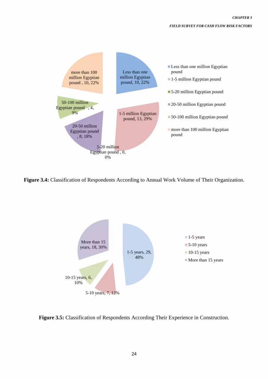
Figure 3.4 illustrates the average annual work load of respondents’ organization.

Figure 3-5 illustrates the previous experience in construction that respondents have. It’s obvious that almost

half of the participants in the category of 1-5 years’ experience.

22

CHAPTER 3

FIELD SURVEY FOR CASH FLOW RISK FACTORS

Figure 3.2: Classification of Respondents According to Their Party Type.

Figure 3.3: Classification of Respondents According to Sector Property.

Contracor, 30, 50%

Client, 10, 17%

Consultant, 20, 33%

Contracor

Client

Consultant

Puplic sector , 12, 20%

Private sector, 48, 80%

Puplic sector

Private sector

23

CHAPTER 3

FIELD SURVEY FOR CASH FLOW RISK FACTORS

Figure 3.4: Classification of Respondents According to Annual Work Volume of Their Organization.

Figure 3.5: Classification of Respondents According Their Experience in Construction.

Less than one million Egyptian pound, 10, 22%

1-5 million Egyptian pound, 13, 29%

5-20 million Egyptian pound , 0,

0%

20-50 million Egyptian pound

, 8, 18%

50-100 million Egyptian pound , 4,

9%

more than 100 million Egyptian pound , 10, 22%

Less than one million Egyptianpound

1-5 million Egyptian pound

5-20 million Egyptian pound

20-50 million Egyptian pound

50-100 million Egyptian pound

more than 100 million Egyptianpound

1-5 years, 29, 48%

5-10 years, 7, 12%

10-15 years, 6, 10%

More than 15 years, 18, 30%

1-5 years

5-10 years

10-15 years

More than 15 years

24

CHAPTER 3

FIELD SURVEY FOR CASH FLOW RISK FACTORS

3.3.1 Calculation and Ranking Risk Factors

After receiving questionnaires from respondents the next step is to calculate the relative importance of each

of the twenty seven risk factors. First the score of each factor will be calculated by multiplying the frequency

with the impact weight. The impact weight will be 1 for 5 point, 0.8 for 4 points, 0.6 for 3 points, 0.4 for 2

points and 0.2 for 1 point so the score of each risk factor will be calculated from the following equation:

SCf=Ff xI Wf …………………………..………………………………………. (3.2)

Total SCf=∑ Ff x IWf ……………………….………………………………. .(3.3)

Where

SCf is the factor score

Ff is the frequency score for the corresponding factor

IWf is the impact weight for the corresponding factor

Total SCf is the total factor score

By assigning this equation all factors scoring have been calculated

Table 3.1: Results of Risk Factors Affecting Net Cash Flow

Factor Total Score

Problems with the foundations 95.2

Listed buildings 93

Archaeological remains 78.2

Inclement weather 89.6

Accidents & theft 119

Extent of float in contract schedule 132.2

Receiving interim certificates 158.6

Retention 123

Delays in payments from client 153

Provision for fluctuation payments 137.2

25

CHAPTER 3

FIELD SURVEY FOR CASH FLOW RISK FACTORS

Table 3.1: Results of Risk Factors Affecting the Net Cash Flow (Continued)

Factor Total Score

Changes in currency exchange rates 113.4

Strikes 109

Level of inflation 116.4

Changes in interest rates 67.2

Estimating error 117.6

Penalty due to the violation of Authority regulation and rules 94.2

Provision for interim certificate 129.4

Material delay 125.2

Error in execution & rework 95.2

Equipment breakdown 99.2

Bankruptcy of subcontractor 83.8

Tender unbalancing 94.6

Consultant’s Instructions 149.8

Agreeing interim valuations on site 171

Delay in agreeing variation 140.4

Delay in settling claims 133.8

Provisions for phased handover 147.4

The max score is calculated as illustrated above by applying equation 3.4. The total score for the factors were

calculated (Table 3.1). Factors are arranged in descending order (as shown in Table 3.2) according to their

Importance index. Such index is calculated by dividing the total score of each factor by the available max

score. This max score can be calculated as:

The max score = max frequency x max impact weight x No of respondents …. (3.4)

The max score = 5 x 1 x 60 = 300 points.

26

CHAPTER 3

FIELD SURVEY FOR CASH FLOW RISK FACTORS

Table 3.2: Ranked Risk Factors Affecting Net Cash Flow (Overall Ranking)

Factor Total Score

Importance

Index

Agreeing interim valuations on site 171 57.0%

Receiving interim certificates 158.6 52.9%

Delays in payments from client 153 51.0%

Consultant’s Instructions 149.8 49.9%

Provisions for phased handover 147.4 49.1%

Delay in agreeing variation 140.4 46.8%

Provision for fluctuation payments 137.2 45.7%

Delay in settling claims 133.8 44.6%

Extent of float in contract schedule 132.2 44.1%

Provision for interim certificate 129.4 43.1%

Material delay 125.2 41.7%

Retention 123 41.0%

Accidents & theft 119 39.7%

Estimating errors 117.6 39.2%

Level of inflation 116.4 38.8%

Changes in currency exchange rates 113.4 37.8%

Strikes 109 36.3%

Equipment breakdown 99.2 33.1%

Problems with the foundations 95.2 31.7%

27

CHAPTER 3

FIELD SURVEY FOR CASH FLOW RISK FACTORS

Table 3.2: Ranked Risk Factors Affecting the Net Cash Flow (Overall Ranking) (Continued)

From Table 3.3 it was seen that the ranking of the risk factors with the respect to work respondent’s

categorization. For an example the factor “level of inflation” has an approximately agreement from the three

parties for example, it ranked 14th overall while it ranked 13th, 15th and 15th for contractor, consultant and

Owner respectively. “Changes in interest rates” has a totally agreement to elaborate more, it ranked 27th

overall while it ranked 27th, 27th and 27th for contractor, consultant and owner respectively. On the other

side, other factors as “material delay” ranked 7th overall while it ranked 14th, 8th and 10th for contractor,

consultant and owner respectively. It’s obvious that the judging differs from party to party depends on factor

and how this party familiar with and how it affect from their point of view.

Four risk factors were found to have near importance index, delay in agreeing variation, accidents & theft,

inclement weather and changes in interest rates. Those risk factors have nearly the same importance index

among contractor, consultant and owner which indicates that they have the same influence from their point

of view.

Thereafter, it was supposed to decide which of the twenty seven factors to be taken into consideration in the

prediction of the cash flow. The percentages obtained for each factor shown in Table 3.2 were summed and

divided by the number of factors to determine the average percentage (Ap) of the factors. Then, the

percentage of each factor was compared with the average percentage. Factors with percentages more than or

Factor Total Score Importance

Index Error in execution & rework 95.2 31.7%

Tender unbalancing 94.6 31.5%

Penalty due to the violation of Authority regulation and rules 94.2 31.4%

Listed buildings 93 31.0%

Inclement weather 89.6 29.9%

Bankruptcy of subcontractor 83.8 27.9%

Archaeological remains 78.2 26.1%

Changes in interest rates 67.2 22.4%

28

CHAPTER 3

FIELD SURVEY FOR CASH FLOW RISK FACTORS

equal to the average percentage were considered as an important factor, while the others were not

considered. The average percentage is determined as follows:

Ap=(57+53+51+50+49+47+46+45+44+43+42+41+40+39+39+38+36+33+32+32+

32+31+31+30+28+26+22 ) / 27 = 39.2 %

Therefore, factors with percentage more than or equal 39.2% were important. Table 3.4 shows the most

important factors that will be taken into consideration.

Table 3.4 presents the most important factor with their total score and importance index. These 14 factors that

were found to be the most importance factors that affect the cash flow analysis according to their importance

index. It was found that the highest importance index factor is related to the relation between consultant and

contractor.

29

CHAPTER 3

FIELD SURVEY FOR CASH FLOW RISK FACTORS

Table 3.3: Ranking of Risk Factors Affecting Net Cash Flow (Respondents Categories)

Risk Factor Overall% Overall

Rank Contractor%

Contractor

rank Consultant%

Consultant

rank

Owner

% owner Rank

Problems with the foundations 31.7% 19 27.9% 24 36.8% 17 33.2% 20

Listed buildings 31.0% 23 27.1% 25 40.2% 12 24.4% 26

Archaeological remains 26.1% 26 27.1% 26 22.6% 26 30.0% 24

Inclement weather 29.9% 24 31.5% 19 27.8% 23 29.2% 25

Accidents & theft 39.7% 13 39.6% 11 38.8% 13 41.6% 11

Extent of float in contract schedule 44.1% 9 41.2% 9 41.6% 11 57.6% 3

Receiving interim certificates 52.9% 2 59.7% 1 45.8% 7 46.4% 9

Retention 41.0% 12 39.3% 12 36.8% 16 54.4% 4

Delays in payments from client 51.0% 3 47.3% 6 53.0% 4 58.0% 2

Provision for fluctuation payments 45.7% 7 36.9% 15 57.4% 2 48.8% 8

Changes in currency exchange rates 37.8% 16 40.9% 10 34.6% 19 34.8% 19

Strikes 36.3% 17 29.6% 20 38.6% 14 52.0% 6

Level of inflation 38.8% 15 38.9% 13 38.2% 15 39.6% 15

30

CHAPTER 3

FIELD SURVEY FOR CASH FLOW RISK FACTORS

Table 3.3: Ranking of Risk Factors Affecting Net Cash Flow Respondents Categories (Continued)

Changes in interest rates 22.4% 27 23.2% 27 22.0% 27 20.8% 27

Estimating error 39.2% 14 35.1% 17 35.2% 18 59.6% 1

Penalty due to the violation of

Authority regulation and rules 31.4% 22 29.1% 22 30.2% 21 40.8% 12

Provision for interim certificate 43.1% 10 47.6% 5 42.4% 10 31.2% 23

Material delay 41.7% 11 38.3% 14 44.6% 8 46.4% 10

Error in execution & rework 31.7% 20 34.1% 18 26.2% 24 35.6% 17

Equipment breakdown 33.1% 18 35.9% 16 28.8% 22 33.2% 21

Bankruptcy of subcontractor 27.9% 25 29.6% 21 22.8% 25 33.2% 22

Tender unbalancing 31.5% 21 29.1% 23 30.6% 20 40.8% 13

Consultant’s Instructions 49.9% 4 49.9% 4 57.4% 3 35.2% 18

Agreeing interim valuations on site 57.0% 1 54.27% 2 62.80% 1 53.60% 5

Delay in agreeing variation 46.8% 6 46.93% 7 44.40% 9 51.20% 7

Delay in settling claims 44.6% 8 42.00% 8 50.60% 5 40.40% 14

Provisions for phased handover 49.1% 5 51.73% 3 50.20% 6 39.20% 16

31

CHAPTER 3

FIELD SURVEY FOR CASH FLOW RISK FACTORS

Table 3.4: The Most Important Factors Affecting Net Cash Flow

Factor Total Score % Agreeing interim valuations on

171 57.0% Receiving interim certificates 158.6 52.9%

Delays in payments from client 153 51.0%

Consultant’s Instructions 149.8 49.9%

Provisions for phased handover 147.4 49.1%

Delay in agreeing variation 140.4 46.8%

Provision for fluctuation payments 137.2 45.7%

Delay in settling claims 133.8 44.6%

Extent of float in contract

132.2 44.1%

Provision for interim certificate 129.4 43.1%

Material delay 125.2 41.7%

Retention 123 41.0%

Accidents & theft 119 39.7%

Estimating error 117.6 39.2%

3.4 Summary and Conclusion

In this chapter fourteen risk factors from twenty seven risk factors were identified to be the most important

factors affecting the project-level cash flow. This step was chosen based on the opinions of sixty respondents

throughout a questionnaire survey. These factors were agreeing interim valuations on site, receiving interim

certificates, delays in payments from client, consultant’s Instructions, provisions for phased handover, delay

in agreeing variation, provision for fluctuation payments, delay in settling claims, and extent of float in

contract schedule, provision for interim certificate, material delay, retention, Accidents & theft and Estimating

error.

Later on the next chapters it is planned to incorporate the effect of these factors in the project cash flow through

a probabilistic cash flow model.

32

CHAPTER 4 PROBABILISTIC CASH FLOW RISK MODEL

CHAPTER 4 PROBABILISTIC CASH FLOW RISK MODEL

4.1 Introduction

This chapter explains the incorporation of the previously identified risk factors into construction project cash flow. In

this chapter the effect of these factors on the different cash flow elements will be investigated. Among these elements

are cash out, cash in, net cash flow and cost of finance. This will be through the development of a probabilistic model

for cash flow prediction.

4.2 Structure of the Model

In this chapter two commercial software will be utilized, which are commonly used in the construction

industry; “primavera p6 professional p6.1” and “primavera risk analysis”. The first one is used as a

planning and scheduling tool while the second is used as a risk management tool. The first software

provides the planner with simple data entry of the activities; dependencies, relationships, duration…etc.

This software performs CPM calculations on the project as well as representing the project schedule in the

form of a bar chart and network diagrams. The second software allows modeling more complex

calculation using VBA (Visual Basic in Application) by implementing the risk factors on the cash out only

so we will not be able to implement the risk factors upon the cash in profile. Consequently, a separate

model will be developed to incorporate the effect of these risk factors in the cash in profile. Microsoft

Excel was used to complete our modeling system outputs by generating cash in, net cash flow and

overdraft profiles.

4.3 Implementation Details

The implementation mechanism consists of three stages (Fig 4.1). The first stage is the planning and scheduling which

is performed by one of the planning programs as primavera p6, Microsoft project 2010 and etc. (in this research

primavera p6 is used for its wide commercial use). The second stage is the implementation of risk factors to the cash

out. This stage is performed by using any risk analysis simulation program as primavera risk analysis, @risk, etc. to get

probabilistic cash out. In this research primavera risk analysis was used as it is the highly skilled and powerful software

and finally it’s more compatible with the primavera p6. The third stage is to develop cash in model through an excel-

macro sheet to get probabilistic cash in, net cash flow and the overdraft calculation.

The first stage inputs are the project activities with their dependencies, relationships, duration, resources and costs to

get the project total duration and cost as cash out S curve. At this stage the project is broken down into activities with

their dependencies, after that cost estimate should be done to determine different type of resources identified by cost

and quantity with the project assignment to the activities. Resource assignment should be assigned with respect to time

cost and performance. Figure 4.2 and Fig 4.3 illustrate the whole stage.

33

CHAPTER 4 PROBABILISTIC CASH FLOW RISK MODEL

The second stage is the implementation of the previously identified risk factors on the cash flow curve results from the

previous stage to get a probabilistic cash out. In this stage, the primavera risk analysis is used. The first step in this stage

is to import the project files from primavera P6 with all its data. Then to build risk register of the classified risk factors

that have been mentioned previously with their impact and probability. These impact and probability were calculated

based on the results of the previous questionnaire survey (Table 4.1).

Table 4.1: Average Probability and Impact for Selected Risk Factors

No Factor Frequency Impact

1 Accidents & theft Medium Medium

2 Extent of float in contract schedule Medium High

3 Receiving interim certificates Medium High

4 Retention Medium Medium

5 Delays in payments from client High High

6 Provision for fluctuation payments Medium High

7 Estimating error Medium High

8 Provision for interim certificate Medium Medium

9 Material delay Medium High

10 Consultant’s Instructions Medium High

11 Agreeing interim valuations on site High High

12 Delay in agreeing variation Medium High

13 Delay in settling claims Medium High

14 Provisions for phased handover High High

According to Fig 4.1, the third stage using the cash in model developed using the Microsoft excel macro sheet to

calculate the cash in, net cash flow and overdraft calculations and simulate their curves.

In the designed macro sheet the inputs are the probabilistic cash out data and the desirable percentage of markup,

overheads, down payment and the monthly interest rate then these inputs goes throw the mathematical model equations

in the macro sheet. The equations are illustrated below:

Pt = Ct *(1+M)*(1-R) ………………………………………………………….. (4.1)

Where,

Pt Cash in at time “t”

Ct Cash out at time “t” 34

CHAPTER 4 PROBABILISTIC CASH FLOW RISK MODEL

M Markup percentage

R Retention Percentage

NSTCHt(1) = ∑ 𝐶𝐶𝐶𝐶 −𝑡𝑡𝑖𝑖=1 ∑ 𝑃𝑃𝐶𝐶 𝑡𝑡−1

𝑖𝑖=1 + ∑ 𝐹𝐹𝐶𝐶𝐹𝐹𝑡𝑡−1𝑖𝑖=1 …………………………………………………… (4.2)

NSTCHt(2) = NSTCHt(1) - Pt ………………………………………………….…………… (4.3)

FCt = NSTCHt(1) * i

Where,

NSTCHt(1) Net cash flow at time “t”, just before last payment

NSTCHt(2) Net cash flow at time “t”, just after last payment

FCt Cost of finance at time “t”

Figure 4.1: Risk Model Stages

Planning & Scheduling WBS Activities relationships and Duration Resource allocation

Cash out C

urve

Implementation of Risk Factors to the resultant Cash out Building Risk register with risk factors and their

probability and impact Assigning risk register to the project

Probabilistic C

ash out

Applying Excel Macro Sheet to Get: Probabilistic Cash in Probabilistic net cash flow Cost of finance

35

CHAPTER 4 PROBABILISTIC CASH FLOW RISK MODEL

After running the macro sheet designed with the previous mathematical model, the output data probabilistic cash

in, probabilistic net cash flow and cost of finance are generated with a schedule graphical representation.

Figure 4.2: Planning and Scheduling Stage

Figure 4.3: Inputs and Outputs in Planning and Scheduling Stage

WBS Breaking down the project to

activities with their dependences

Cost estimate Determining activities duration, Resources with their cost and

Resource allocation Resource assigned to the activities with respect to project constrains

Planning and

scheduling process

Activities, Durations, Dependences,

Resources and Cost Cost S-curve (Cash out)

36

CHAPTER 4 PROBABILISTIC CASH FLOW RISK MODEL

4.4 Example for Model Testing and Verification

In order to examine the proposed system and test its capabilities to model probabilistic cash flow, an example

project a building extension consisting of eleven activities was used. .Table 4.2 illustrates the project data.

Table 4.2: Activities Relationship, Cost and Duration

Activity ID Activity Name Predecessor Cost Duration

A1000 Site excavation None 114800 10

A1010 PC-Foundation A1000 200850 2

A1020 First Stage Isolation A1010 214720 8

A1030 Second Stage Isolation A1020 &A1060 80427 14

A1040 RC-Foundation A1020 639955 22

A1050 RC-RW & Col Level 1 A1010 394460 18

A1060 RC-Slab - Level 1 A1050 395395 18

A1070 RC-RW & Col Level 2 A1030 394460 18

A1080 RC-Slab - Level 2 A1070 395395 18

A1090 Backfilling A1080 19710 7

A1100 poly Sheets with 5cm PC A1090 71070 5

The project has been worked out with primavera p6 at the first stage and was found to have an estimated cost

of 2,921,242 EGP and a duration of 180 days or 6 months.

The second stage started with exporting project data to primavera risk analysis and start with building risk

register for the project. Risk register uses the previously identified risk factors with their corresponding

probability and impact that has been previously determined based on the questionnaire survey.

Then such risk factors were assigned to the corresponding activity. This process was done by experience of

the top management head or by a brain storming sessions with the management team. After that risk analysis

was used with the desired number of iterations. The output data from this software is probabilistic date with

respect time and cost. Figure 4.4 to 4.6 illustrate the program outcome in the form of probability distribution.

The graphs illustrate the number of iteration hits for each probability.

37

CHAPTER 4 PROBABILISTIC CASH FLOW RISK MODEL

Figure 4.4 shows the project duration was found to be 180, 287 and 355 days at corresponding probabilities

of 0%, 50 %, and 100% respectively while Figure 4.5 Cost shows the project cost for a probability of 0%,

50 %, and 100% to be 2,921,242EP, 4,720,617EP and 6, 926,010EP respectively.

Figure 4.7 represents the probabilistic cash out for the project with probability 0%, 50 %, 100% (For Both

cost and time) as 2,921,242EP, 4,720,617EP and 6,926,010EP respectively and 180,287 and 355 days

respectively. From this figure, it’s obvious that the mean value of this probabilistic cash out is in the same line

with the deterministic value but with an increase in cost and time which really happen in the real life project.

This project has been executed and finished before this study, so the final cost and time data are available.

The project has been completed in 350 days and with actual cost of 3,005,440 EGP. The corresponding

probability for this duration and cost is 97% and 2% respectively.

The bars in Figures 4.4 to 4.6 illustrate the number of iteration that give this probability. As in Figure 4.4 the

corresponding number of iteration for probability 50% is 130 iteration.

It’s logic for duration to be with this value as the most of construction projects are completed after their

scheduled time, but contractor is very interested in the cost control so the cost overrun may not be more than

5% .

Figure 4.4: Duration Probability Distribution

200 250 300 350

Distribution (start of interval)

0

20

40

60

80

100

120

140

Hits

0% 180

5% 243

10% 252

15% 262

20% 265

25% 271

30% 276

35% 279

40% 283

45% 285

50% 287

55% 291

60% 292

65% 294

70% 298

75% 301

80% 305

85% 308

90% 313

95% 321

100% 355

Cum

ulat

ive

Freq

uenc

y

38

CHAPTER 4 PROBABILISTIC CASH FLOW RISK MODEL

Figure 4.5: Cost Probability Distribution

Figure 4.6: Finish Date Probability Distribution

$3,000,000 $4,000,000 $5,000,000 $6,000,000 $7,000,000

Distribution (start of interval)

0

20

40

60

80

100

120

140Hi

ts

0% $2,921,242

5% $3,680,058

10% $3,899,942

15% $4,078,056

20% $4,186,055

25% $4,286,243

30% $4,393,853

35% $4,495,376

40% $4,584,440

45% $4,656,570

50% $4,752,947

55% $4,857,236

60% $4,942,546

65% $5,046,316

70% $5,133,325

75% $5,217,640

80% $5,371,560

85% $5,526,807

90% $5,740,594

95% $5,969,058

100% $6,926,010

Cum

ulat

ive

Freq

uenc

y

09/09/2013 29/10/2013 18/12/2013 06/02/2014

Distribution (start of interval)

0

20

40

60

80

100

120

140

Hits

0% 28/08/2013

5% 30/10/2013

10% 08/11/2013

15% 18/11/2013

20% 21/11/2013

25% 27/11/2013

30% 02/12/2013

35% 05/12/2013

40% 09/12/2013

45% 11/12/2013

50% 13/12/2013

55% 17/12/2013

60% 18/12/2013

65% 20/12/2013

70% 24/12/2013

75% 27/12/2013

80% 31/12/2013

85% 03/01/2014

90% 08/01/2014

95% 16/01/2014

100% 19/02/2014

Cum

ulat

ive

Freq

uenc

y

39

CHAPTER 4 PROBABILISTIC CASH FLOW RISK MODEL

Figure 4.7: Probabilistic Cash Out

The third and last stage of this system is the cash in model that have been developed through the excel macro

sheet which will calculate the cash in, net cash flow and the overdraft calculations. Microsoft excel was used

as a tool of getting such calculations outputs and for graphical representation.

The input of this stage is the output from the previous stage, probabilistic cash out (Table 4.3)and some other

variables as markup, monthly interest value, percentage of down payment ( if any ) and retention. From the

probabilistic cash out we get monthly cost then it goes through the designed mathematical model.

Table 4.3: Monthly Cost Probability Distribution

Month P0 P50 P100 0 0 0 0 1 243006 511841 773315 2 511259 575104 670904 3 481055 529764 705342 4 395955 460034 658583 5 354807 480382 528858 6 360197 439109 726799 7 352732 530286 741898 8 222231 477078 624255 9 0 498992 745385 10 0 218027 702201 11 0 0 48470

12/04/2013 01/06/2013 21/07/2013 09/09/2013 29/10/2013 18/12/2013 06/02/2014

Time

0

1,000,000

2,000,000

3,000,000

4,000,000

5,000,000

6,000,000

7,000,000

Cu

mu

lati

ve

Scheduled Mean P0 P50 P100

40

CHAPTER 4 PROBABILISTIC CASH FLOW RISK MODEL

This mathematical model used to calculate the monthly cash in and the net cash flow. The model can also used

to calculate the overdraft values as well as the corresponding finance cost if there is any external source of

finance.

To calculate the cash in of this example application some assumption should be made. Such

variables mainly include

Markup = 20%, Retention = 10%, Down payment=10%, Monthly interest rate = 1%

The calculated monthly cash in is shown in Table 4.4.

Table 4.4: Cash in Probability Distribution

Month P0 P50 P100 0 350,549 566,474 831,121

1 0 0 0

2 233,286 491,367 742,382

3 490,809 552,100 644,068

4 461,813 508,573 677,128

5 380,117 441,633 632,240

6 340,615 461,167 507,704

7 345,789 421,545 697,727

8 338,623 509,075 712,222

9 563,891 457,995 599,285

10 479,032 715,570

11 775,780 674,113

12 877,652

Then the next step is to calculate the overdraft requirement for various probability values with a monthly

interest assumption of 1% in (Tables 4.5 to 4.7).

41

CHAPTER 4 PROBABILISTIC CASH FLOW RISK MODEL

Table 4.5: Overdraft Calculation for Probability 0%

P 0% Month Expenses Payment Overdraft interest total

0 0 350,549 0 0 0 1 243,006 0 -107,543 0 -107,543 2 511,259 233,286 403,716 4,037 407,753 3 481,055 490,809 655,522 6,555 662,078 4 395,955 461,813 567,224 5,672 572,896 5 354,807 380,117 465,890 4,659 470,549 6 360,197 340,615 450,629 4,506 455,136 7 352,732 345,789 467,253 4,673 471,926 8 222,231 338,623 348,367 3,484 351,851 9 0 563,891 13,228 132 13,361 10 0 0 -550,530 0 -550,530 11 0 0 0 0 12 0 0 0 0 33,718

Table 4.6: Overdraft Calculation for Probability 50%

P 50% Month Expenses Payment Overdraft interest total

0 0 566,474 0 0 0 1 511,841 0 -54,633 0 -54,633 2 575,104 491,367 520,471 5,205 525,676 3 529,764 552,100 564,072 5,641 569,713 4 460,034 508,573 477,647 4,776 482,424 5 480,382 441,633 454,232 4,542 458,775 6 439,109 461,167 456,251 4,563 460,813 7 530,286 421,545 529,933 5,299 535,232 8 477,078 509,075 590,765 5,908 596,673 9 498,992 457,995 586,590 5,866 592,456 10 218,027 479,032 352,489 3,525 356,013 11 0 775,780 -123,019 0 -123,019 12 0 0 -898,799 0 -898,799 45,325

42

CHAPTER 4 PROBABILISTIC CASH FLOW RISK MODEL

Table 4.7: Overdraft Calculation for Probability 100%

P 100% Month Expenses Payment Overdraft interest total

0 0 831,121 0 0 0 1 773,315 0 -57,806 0 -57,806 2 670,904 742,382 613,098 6,131 619,229 3 705,342 644,068 582,188 5,822 588,010 4 658,583 677,128 602,525 6,025 608,551 5 528,858 632,240 460,280 4,603 464,883 6 726,799 507,704 559,442 5,594 565,037 7 741,898 697,727 799,231 7,992 807,224 8 624,255 712,222 733,751 7,338 741,089 9 745,385 599,285 774,252 7,743 781,994 10 702,201 715,570 884,911 8,849 893,760 11 48,470 674,113 226,660 2,267 228,927 12 877,652 -445,186 0 -445,186 13 -1,322,839 0 -1,322,839 62,363

The finance cost for the 0 %, 50%and 100% was 33,718, 45,325 and 62,363 respectively. The last output of

the cash in model is the graphical representation shown in (Figures 4.8 to 4.10). The graphs illustrate the cash

in, cash out and net cash flow individually.

Figure 4.8: Cash Flow for Probability 0%

2,921,242

3,505,490

584,248

-1,000,000-500,000

0500,000

1,000,0001,500,0002,000,0002,500,0003,000,0003,500,0004,000,000

0 5 10 15

Cash

Month

P 0 %

cash-out

Cash-in

Net-cash

43

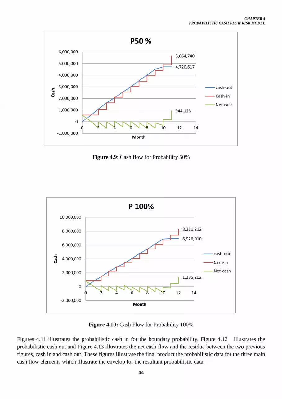
CHAPTER 4 PROBABILISTIC CASH FLOW RISK MODEL

Figure 4.9: Cash flow for Probability 50%

Figure 4.10: Cash Flow for Probability 100%

Figures 4.11 illustrates the probabilistic cash in for the boundary probability, Figure 4.12 illustrates the probabilistic cash out and Figure 4.13 illustrates the net cash flow and the residue between the two previous figures, cash in and cash out. These figures illustrate the final product the probabilistic data for the three main cash flow elements which illustrate the envelop for the resultant probabilistic data.

4,720,617

5,664,740

944,123

-1,000,000

0

1,000,000

2,000,000

3,000,000

4,000,000

5,000,000

6,000,000

0 2 4 6 8 10 12 14

Cash

Month

P50 %

cash-out

Cash-in

Net-cash

6,926,010

8,311,212

1,385,202

-2,000,000

0

2,000,000

4,000,000

6,000,000

8,000,000

10,000,000

0 2 4 6 8 10 12 14

Cash

Month

P 100%

cash-out

Cash-in

Net-cash

44

CHAPTER 4 PROBABILISTIC CASH FLOW RISK MODEL

Figure 4.11: Probabilistic Cash In

Figure 4.12: Probabilistic Cash Out

3,505,490

5,664,740

8,311,212

0

1,000,000

2,000,000

3,000,000

4,000,000

5,000,000

6,000,000

7,000,000

8,000,000

9,000,000

0 2 4 6 8 10 12 14

Cash

Month

Probabilistic Cash in

P0 Cash-in

P50 Cash-in

P100 Cash-in

2,921,242

4,720,617

6,926,010

0

1,000,000

2,000,000

3,000,000

4,000,000

5,000,000

6,000,000

7,000,000

8,000,000

0 2 4 6 8 10 12

Cash

Month

Probabilistic cash out

P0

P50

P100

45

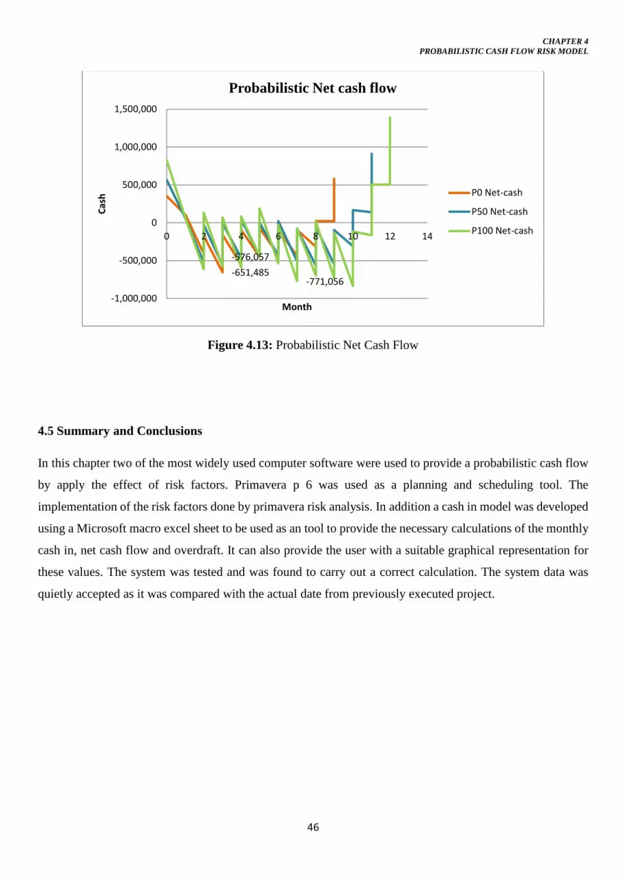
CHAPTER 4 PROBABILISTIC CASH FLOW RISK MODEL

Figure 4.13: Probabilistic Net Cash Flow

4.5 Summary and Conclusions

In this chapter two of the most widely used computer software were used to provide a probabilistic cash flow

by apply the effect of risk factors. Primavera p 6 was used as a planning and scheduling tool. The

implementation of the risk factors done by primavera risk analysis. In addition a cash in model was developed

using a Microsoft macro excel sheet to be used as an tool to provide the necessary calculations of the monthly

cash in, net cash flow and overdraft. It can also provide the user with a suitable graphical representation for

these values. The system was tested and was found to carry out a correct calculation. The system data was

quietly accepted as it was compared with the actual date from previously executed project.

-651,485-576,057

-771,056

-1,000,000

-500,000

0

500,000

1,000,000

1,500,000

0 2 4 6 8 10 12 14

Cash

Month

Probabilistic Net cash flow

P0 Net-cash

P50 Net-cash

P100 Net-cash

46

CHAPTER 5 CASE STUDY APPLICATION

CHAPTER 5

CASE STUDY APPLICATION

5.1 Introduction

In the previous chapter the designed model was tested through a small example project with a full data to

confirm that the model can correctly carry out the different cash flow calculations. A case study of real life

project will be presented in this chapter as an application of the proposed cash flow model. The objective of

this case study is to investigate the ability of the proposed model to provide a reliable forecasting of the

different cash flow elements on a large scale project.

5.2 Case Study

5.2.1 Project Description

This project is one building of the German University project in Cairo located in the 5th settlement, built on an

area of 1200 m². This project is an educational building consists of 5 typical floors, each contains 4 classrooms

and an auditorium. It is constructed as a steel structure to get some benefits as: salvage value, long spans, and

quick installation, easy for further replacement in contrary of concrete structures. The project consists of 147

activities with a total estimated duration of 451 days and an estimated cost of 30,479277 EGP.

5.2.2 Planning and Scheduling

The project has been broken down to activities with their dependencies and relations as illustrated

in appendix B. After that those date entered on primavera p6 with the sot date and resources and

it found that the project consists of 147 activities with a total estimated duration of 451 days and

an estimated cost of 30,479,277 EGP.

5.2.3 Risk Implementation The second stage is the risk implementation process that was started now after finishing the

planning and scheduling stage with their output and the corresponding risk data mentioned

before.

47

CHAPTER 5 CASE STUDY APPLICATION

The risk register of the primavera risk analysis was assigned to each activity. The risk register

itself does not change from project to anther it is only the assignment of the risks to the

activities. Then the risk plan was carried out.

The results of this risk analysis are shown in the form of probability distribution for both cost and

time. Figure 5.1 shows the expected duration probability of 0%, 50 %, and 100% was 451, 538

and 631 days respectively. Moreover, Figure 5.2 presents the expected cost of 30,488,460 EGP,

31,952,106 EGP and 33,894,665 EGP at corresponding probability of 0%, 50 %, and 100%

respectively. Figure 5.3 represent the probabilistic finish date.

The next step is the application of cash in model developed with Microsoft macro excel. For this

step the input data will be the probabilistic data from the previous step. These data are the

corresponding cost and duration for probability 0%, 50% and 100 % to build the cash in and net

cash curves. For the validation example at the studied probability points of the corresponding cost

and duration have been met. It differs in this example where for the max cost (33,894,665EGP)

the corresponding duration was 540 days which stand for the probability of 50%. On the other

side the 50% probability cost (31,952,106EGP) has a total duration of 630 days which correspond

for 100 % of duration probability. The min cost probability at 0 % (30,488,460EGP) where the

corresponding duration is 600 days with probability 85 %.

So to cover all the expected different scenarios for both cost and time, several combination of

alternatives for the expected cost and time were investigated. The results of these cases were

shown in Figures 5.2, 5.3 and 5.4. So five different alternatives were studied with different

probability for cost and time. As an example the first alternative named P (0, 85) were 0 % is

corresponding probability for cost and 85 % is corresponding for time.

48

CHAPTER 5 CASE STUDY APPLICATION

Figure 5.1: Duration Probability Distribution

Figure 5.2: Cost Probability Distribution

500 550 600

Distribution (start of interval)

0.0

10.0

20.0

30.0

40.0

50.0

60.0

Hits

0% 451

5% 471

10% 481

15% 488

20% 495

25% 500

30% 507

35% 514

40% 520

45% 528

50% 538

55% 545

60% 553

65% 562

70% 572

75% 581

80% 588

85% 595

90% 601

95% 610

100% 631

Cum

ulati

ve F

requ

ency

Entire Plan : Duration

$31,000,000 $32,000,000 $33,000,000 $34,000,000

Distribution (start of interval)

0

20

40

60

80

100

120

140

160

180

Hits

0% $30,488,460

5% $31,027,612

10% $31,235,595

15% $31,366,075

20% $31,455,139

25% $31,572,105

30% $31,657,047

35% $31,732,595

40% $31,808,018

45% $31,871,999

50% $31,952,106

55% $32,041,723

60% $32,123,685

65% $32,205,251

70% $32,302,057

75% $32,382,143

80% $32,483,341

85% $32,619,857

90% $32,748,047

95% $32,989,890

100% $33,894,665

Cumu

lative

Freq

uenc

y

g ( g )Entire Plan : Cost

49

CHAPTER 5 CASE STUDY APPLICATION

Figure 5.3: Finish Date Probability Distribution

Figure 5.4: Probabilistic Cash Out

25/03/2014 14/05/2014 03/07/2014 22/08/2014

Distribution (start of interval)

0.0

10.0

20.0

30.0

40.0

50.0

60.0

Hits

0% 27/03/2014

5% 16/04/2014

10% 26/04/2014

15% 03/05/2014

20% 10/05/2014

25% 15/05/2014

30% 22/05/2014

35% 29/05/2014

40% 04/06/2014

45% 12/06/2014

50% 22/06/2014

55% 29/06/2014

60% 07/07/2014

65% 16/07/2014

70% 26/07/2014

75% 04/08/2014

80% 11/08/2014

85% 18/08/2014

90% 24/08/2014

95% 02/09/2014

100% 23/09/2014

Cumu

lative

Freq

uenc

y

Entire Plan : Finish Date

18/02/2013 09/04/2013 29/05/2013 18/07/2013 06/09/2013 26/10/2013 15/12/2013 03/02/2014 25/03/2014 14/05/2014 03/07/2014 22/08/2014

Time

0

5,000,000

10,000,000

15,000,000

20,000,000

25,000,000

30,000,000

35,000,000

Cu

mu

lati

ve

Resource Flow for CostFilter: Entire Plan

Scheduled Mean P0 P50 P70 P100

50

CHAPTER 5 CASE STUDY APPLICATION

The next step is to use the developed cash in model to obtain the cash flow data that cannot be

obtained from the primavera risk analysis. In this stage the inputs are the output data from the

previous stage with additional variables. Such variables mainly include

Markup = 20%, Retention = 10%, Down payment = 10%, Monthly interest rate = 1%

The output of this stage will be the cash in, net cash flow and overdraft calculation for the five

alternatives that were mentioned and defined above.

Table 5.1 illustrates the monthly cost for the five alternatives where Table 5.2 illustrates the

cumulative costs.

Table 5.1: Monthly Costs

Month P(0,85) P(50,100) P(100,50) P(70,70) Deterministic 0 0 0 0 0 0

1 1,480,645 1,530,000 1,530,000 1,480,645 1,530,000

2 509,483 504,923 532,000 535,141 532,000

3 189,974 480,174 1,407,280 369,535 805,264

4 437,754 1,181,921 2,288,405 1,035,663 1,964,208

5 834,288 1,670,092 2,658,057 1,286,934 2,948,058

6 1,764,508 1,546,038 1,172,913 1,452,605 1,316,433

7 794,067 2,321,490 3,302,698 2,521,681 2,156,696

8 2,517,236 1,431,158 1,817,695 932,989 2,949,607

9 546,593 2,034,747 1,608,828 2,358,735 482,035

10 2,692,908 1,562,383 2,342,703 1,019,937 3,012,645

11 547,426 1,746,024 1,122,738 1,917,528 1,525,806

12 1,596,133 2,092,737 1,770,045 1,245,840 1,425,625

13 1,562,343 1,469,882 7,309,881 1,574,786 7,589,233

14 765,792 1,268,253 1,661,050 1,566,916 1,441,667

15 2,326,247 4,063,335 1,395,281 1,115,166 800,000

16 593,071 5,083,136 638,194 1,256,631 0

17 1,515,446 1,114,748 697,986 7,030,491 0

18 3,942,934 427,139 638,911 1,913,885 0

19 4,922,163 281,185 0 840,031 0

20 949,449 128,813 0 0 0

21 0 13,928 0 0 0

51

CHAPTER 5 CASE STUDY APPLICATION

Table 5.3 & Table5.4 represent the cash in calculation as table 5.3 illustrates monthly cash in and table 5.4

illustrates the cumulative cash in.

Table 5.2: Cumulative Costs

Month P(0,85) P(50,100) P(100,50) P(70,70) Deterministic

0 0 0 0 0 0

1 1,480,645 1,530,000 1,530,000 1,480,645 1,530,000

2 1,990,128 2,034,923 2,062,000 2,015,786 2,062,000

3 2,180,102 2,515,097 3,469,280 2,385,321 2,867,264

4 2,617,856 3,697,018 5,757,685 3,420,984 4,831,472

5 3,452,144 5,367,110 8,415,742 4,707,918 7,779,530

6 5,216,652 6,913,148 9,588,655 6,160,523 9,095,963

7 6,010,719 9,234,638 12,891,353 8,682,204 11,252,659

8 8,527,955 10,665,796 14,709,048 9,615,193 14,202,266

9 9,074,548 12,700,543 16,317,876 11,973,928 14,684,301

10 11,767,456 14,262,926 18,660,579 12,993,865 17,696,946

11 12,314,882 16,008,950 19,783,317 14,911,393 19,222,752

12 13,911,015 18,101,687 21,553,362 16,157,233 20,648,377

13 15,473,358 19,571,569 28,863,243 17,732,019 28,237,610

14 16,239,150 20,839,822 30,524,293 19,298,935 29,679,277

15 18,565,397 24,903,157 31,919,574 20,414,101 30,479,277

16 19,158,468 29,986,293 32,557,768 21,670,732

17 20,673,914 31,101,041 33,255,754 28,701,223

18 24,616,848 31,528,180 33,894,665 30,615,108

19 29,539,011 31,809,365 31,455,139

20 30,488,460 31,938,178

21 31,952,106

52

CHAPTER 5 CASE STUDY APPLICATION

Table 5.3: Monthly Cash In

Month P(0,85) P(50,100) P(100,50) P(70,70) deterministic

0 3,658,615 3,834,253 4,067,360 3,774,617 3,657,513

1 0 0 0 0 0

2 1,421,419 1,468,800 1,468,800 1,421,419 1,468,800

3 489,104 484,726 510,720 513,735 510,720

4 182,375 460,967 1,350,989 354,754 773,053

5 420,244 1,134,644 2,196,869 994,236 1,885,640

6 800,916 1,603,288 2,551,735 1,235,457 2,830,136

7 1,693,928 1,484,196 1,125,996 1,394,501 1,263,776

8 762,304 2,228,630 3,170,590 2,420,814 2,070,428

9 2,416,547 1,373,912 1,744,987 895,669 2,831,623

10 524,729 1,953,357 1,544,475 2,264,386 462,754

11 2,585,192 1,499,888 2,248,995 979,140 2,892,139

12 525,529 1,676,183 1,077,828 1,840,827 1,464,774

13 1,532,288 2,009,028 1,699,243 1,196,006 1,368,600

14 1,499,849 1,411,087 7,017,486 1,511,795 7,285,664

15 735,160 1,217,523 1,594,608 1,504,239 1,384,000

16 2,233,197 3,900,802 1,339,470 1,070,559 4,425,513

17 569,348 4,879,811 612,666 1,206,366 0

18 1,454,828 1,070,158 670,067 6,749,271 0

19 3,785,217 410,053 4,680,714 1,837,330 0

20 4,725,276 269,938 0 4,581,046 0

21 4,570,086 123,660 0 0

22 0 3,847,624 0 0 0

53

CHAPTER 5 CASE STUDY APPLICATION

Table 5.4: Cumulative Cash in

Month P(0,85) P(50,100) P(100,50) P(70,70) deterministic

0 3,658,615 3,834,253 4,067,360 3,774,617 3,657,513

1 3,658,615 3,834,253 4,067,360 3,774,617 3,657,513

2 5,080,034 5,303,053 5,536,160 5,196,036 5,126,313

3 5,569,138 5,787,779 6,046,880 5,709,771 5,637,033

4 5,751,513 6,248,746 7,397,869 6,064,525 6,410,087

5 6,171,757 7,383,390 9,594,737 7,058,761 8,295,726

6 6,972,673 8,986,678 12,146,472 8,294,218 11,125,862

7 8,666,601 10,470,875 13,272,469 9,688,719 12,389,638

8 9,428,905 12,699,505 16,443,059 12,109,533 14,460,066

9 11,845,452 14,073,417 18,188,046 13,005,202 17,291,689

10 12,370,181 16,026,774 19,732,521 15,269,588 17,754,442

11 14,955,373 17,526,662 21,981,516 16,248,727 20,646,581

12 15,480,902 19,202,845 23,059,344 18,089,554 22,111,355

13 17,013,190 21,211,872 24,758,587 19,285,560 23,479,955

14 18,513,039 22,622,959 31,776,073 20,797,355 30,765,619

15 19,248,199 23,840,482 33,370,681 22,301,594 32,149,619

16 21,481,396 27,741,283 34,710,151 23,372,154 36,575,132

17 22,050,744 32,621,094 35,322,817 24,578,519

18 23,505,573 33,691,252 35,992,884 31,327,791

19 27,290,789 34,101,306 40,673,598 33,165,120

20 32,016,066 34,371,243 37,746,167

21 36,586,152 34,494,904

22 38,342,527

54

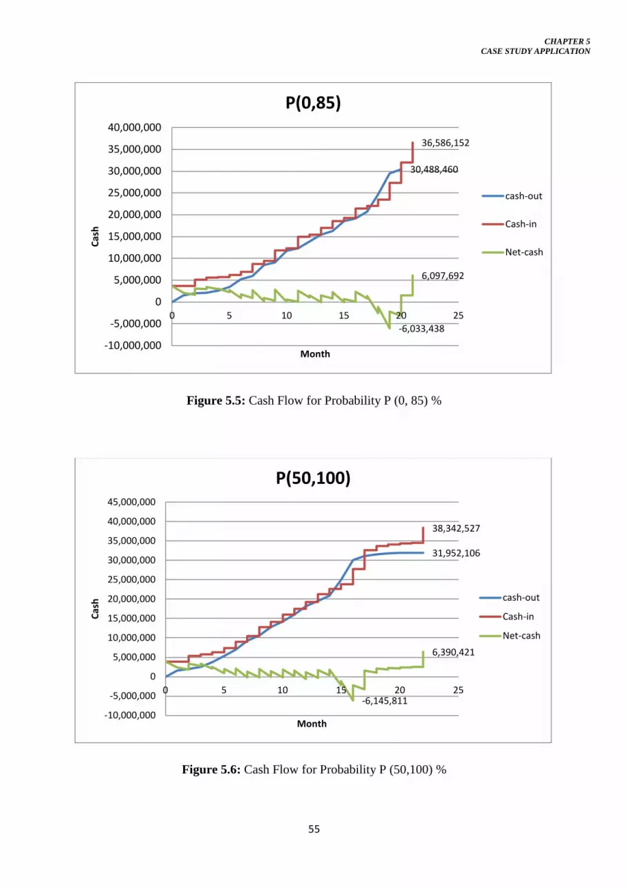
CHAPTER 5 CASE STUDY APPLICATION

Figure 5.5: Cash Flow for Probability P (0, 85) %

Figure 5.6: Cash Flow for Probability P (50,100) %

30,488,460

36,586,152

-6,033,438

6,097,692

-10,000,000

-5,000,000

0

5,000,000

10,000,000

15,000,000

20,000,000

25,000,000

30,000,000

35,000,000

40,000,000

0 5 10 15 20 25

Cash

Month

P(0,85)

cash-out

Cash-in

Net-cash

31,952,106

38,342,527

-6,145,811

6,390,421

-10,000,000

-5,000,000

0

5,000,000

10,000,000

15,000,000

20,000,000

25,000,000

30,000,000

35,000,000

40,000,000

45,000,000

0 5 10 15 20 25

Cash

Month

P(50,100)

cash-out

Cash-in

Net-cash

55

CHAPTER 5 CASE STUDY APPLICATION

Figure 5.7: Cash Flow for Probability P (100, 50) %

Figure 5.8: Cash Flow for Probability P (70, 70) %

33,894,665

40,673,598

6,778,933

-10,000,000

0

10,000,000

20,000,000

30,000,000

40,000,000

50,000,000

0 5 10 15 20 25

Cash

Month

P(100,50)

cash-out

Cash-in

Net-cash

31,455,139

37,746,167

6,291,028

-10,000,000

-5,000,000

0

5,000,000

10,000,000

15,000,000

20,000,000

25,000,000

30,000,000

35,000,000

40,000,000

0 5 10 15 20 25

Cash

Month

P(70,70)

cash-out

Cash-in

Net-cash

56

CHAPTER 5 CASE STUDY APPLICATION

Figure 5.9: Cash Flow for Deterministic Probability

The final step is the overdraft calculation (based on an assumed monthly interest rate of 1%). In this step the

input data are the output data from the cash flow calculation. The following tables illustrate the overdraft

calculations.

Table 5.6 to Table 5.10 illustrate the overdraft for all the single cash flows with their cost of finance which

compose the probabilistic overdraft calculation.

30,479,277

36,575,132

-6,199,322

1,670,3426,095,855

-10,000,000

-5,000,000

0

5,000,000

10,000,000

15,000,000

20,000,000

25,000,000

30,000,000

35,000,000

40,000,000

0 5 10 15 20 25

Cash

Month

Deterministic

cash-out

Cash-in

Net-cash

57

CHAPTER 5 CASE STUDY APPLICATION

Table 5.6: Overdraft Calculation for P (0, 85) %

P (0, 85) %

Month Expenses Payment Overdraft Interest Total

0 0 3,658,615 -3,658,615 0 -3,658,615

1 1,480,645 0 -2,177,970 0 -2,177,970

2 509,483 1,421,419 -1,668,487 0 -1,668,487

3 189,974 489,104 -2,899,932 0 -2,899,932

4 437,754 182,375 -2,951,282 0 -2,951,282

5 834,288 420,244 -2,299,369 0 -2,299,369

6 1,764,508 800,916 -955,105 0 -955,105

7 794,067 1,693,928 -961,954 0 -961,954

8 2,517,236 762,304 -138,646 0 -138,646

9 546,593 2,416,547 -354,357 0 -354,357

10 2,692,908 524,729 -77,996 0 -77,996

11 547,426 2,585,192 -55,299 0 -55,299

12 1,596,133 525,529 -1,044,358 0 -1,044,358

13 1,562,343 1,532,288 -7,544 0 -7,544

14 765,792 1,499,849 -774,040 0 -774,040

15 2,326,247 735,160 52,358 524 52,882

16 593,071 2,233,197 -89,208 0 -89,208

17 1,515,446 569,348 -806,959 0 -806,959

18 3,942,934 1,454,828 2,566,627 25,666 2,592,293

19 4,922,163 3,785,217 6,059,628 60,596 6,120,224

20 949,449 4,725,276 3,284,457 32,845 3,317,301

21 0 4,570,086 -1,407,975 0 -1,407,975

119,631

58

CHAPTER 5 CASE STUDY APPLICATION

Table 5.7: Overdraft Calculation for P (50, 100) %

P (50, 100) %

Month Expenses Payment Overdraft Interest Total

0 0 3,834,253 -3,834,253 0 -3,834,253

1 1,530,000 0 -2,304,253 0 -2,304,253

2 504,923 1,468,800 -1,799,330 0 -1,799,330

3 480,174 484,726 -2,787,956 0 -2,787,956

4 1,181,921 460,967 -2,090,761 0 -2,090,761

5 1,670,092 1,134,644 -881,636 0 -881,636

6 1,546,038 1,603,288 -470,242 0 -470,242

7 2,321,490 1,484,196 247,960 2,480 250,439

8 1,431,158 2,228,630 197,401 1,974 199,375

9 2,034,747 1,373,912 5,491 55 5,546

10 1,562,383 1,953,357 194,018 1,940 195,958

11 1,746,024 1,499,888 -11,375 0 -11,375

12 2,092,737 1,676,183 581,474 5,815 587,289

13 1,469,882 2,009,028 380,988 3,810 384,798

14 1,268,253 1,411,087 -355,977 0 -355,977

15 4,063,335 1,217,523 2,296,271 22,963 2,319,234

16 5,083,136 3,900,802 6,184,847 61,848 6,246,696

17 1,114,748 4,879,811 3,460,642 34,606 3,495,248

18 427,139 1,070,158 -957,423 0 -957,423

19 281,185 410,053 -1,746,396 0 -1,746,396

20 128,813 269,938 -2,027,637 0 -2,027,637

21 13,928 123,660 -2,283,646 0 -2,283,646

22 0 3,847,624 -2,407,307 0 -2,407,307

135,491

59

CHAPTER 5 CASE STUDY APPLICATION

Table 5.8: Overdraft Calculation for P (100, 50) %

P (100, 50) %

Month Expenses Payment Overdraft Interest Total

0 0 4,067,360 -4,067,360 0 -4,067,360

1 1,530,000 0 -2,537,360 0 -2,537,360

2 532,000 1,468,800 -2,005,360 0 -2,005,360

3 1,407,280 510,720 -2,066,880 0 -2,066,880

4 2,288,405 1,350,989 -289,195 0 -289,195

5 2,658,057 2,196,869 1,017,873 10,179 1,028,052

6 1,172,913 2,551,735 4,096 41 4,137

7 3,302,698 1,125,996 755,101 7,551 762,652

8 1,817,695 3,170,590 1,454,350 14,544 1,468,894

9 1,608,828 1,744,987 -92,868 0 -92,868

10 2,342,703 1,544,475 504,847 5,048 509,896

11 1,122,738 2,248,995 88,159 882 89,041

12 1,770,045 1,077,828 -389,909 0 -389,909

13 7,309,881 1,699,243 5,842,143 58,421 5,900,565

14 1,661,050 7,017,486 5,862,371 58,624 5,920,995

15 1,395,281 1,594,608 298,790 2,988 301,778

16 638,194 1,339,470 -654,636 0 -654,636

17 697,986 612,666 -1,296,120 0 -1,296,120

18 638,911 670,067 -1,269,875 0 -1,269,875

19 0 4,680,714 -1,939,941 0 -1,939,941

158,277

60

CHAPTER 5 CASE STUDY APPLICATION

Table 5.9: Overdraft Calculation for P (70, 70) %

P (70, 70) %

Month Expenses Payment Overdraft Interest Total

0 0 3,774,617 -3,774,617 0 -3,774,617

1 1,480,645 0 -2,293,972 0 -2,293,972

2 535,141 1,421,419 -1,758,831 0 -1,758,831

3 369,535 513,735 -2,810,715 0 -2,810,715

4 1,035,663 354,754 -2,288,787 0 -2,288,787

5 1,286,934 994,236 -1,356,607 0 -1,356,607

6 1,452,605 1,235,457 -898,238 0 -898,238

7 2,521,681 1,394,501 387,986 3,880 391,866

8 932,989 2,420,814 -69,646 0 -69,646

9 2,358,735 895,669 -131,725 0 -131,725

10 1,019,937 2,264,386 -7,457 0 -7,457

11 1,917,528 979,140 -354,315 0 -354,315

12 1,245,840 1,840,827 -87,614 0 -87,614

13 1,574,786 1,196,006 -353,655 0 -353,655

14 1,566,916 1,511,795 17,255 173 17,427

15 1,115,166 1,504,239 -379,202 0 -379,202

16 1,256,631 1,070,559 -626,810 0 -626,810

17 7,030,491 1,206,366 5,333,122 53,331 5,386,453

18 1,913,885 6,749,271 6,093,972 60,940 6,154,912

19 840,031 1,837,330 245,672 2,457 248,128

20 0 4,581,046 -1,589,201 0 -1,589,201

120,780

61

CHAPTER 5 CASE STUDY APPLICATION

Table 5.10: Overdraft calculation for Deterministic

Deterministic

Month Expenses Payment Overdraft Interest Total

0 0 3,657,513 -3,657,513 0 -3,657,513

1 1,530,000 0 -2,127,513 0 -2,127,513

2 532,000 1,468,800 -1,595,513 0 -1,595,513

3 805,264 510,720 -2,259,049 0 -2,259,049

4 1,964,208 773,053 -805,561 0 -805,561

5 2,948,058 1,885,640 1,369,443 13,694 1,383,138

6 1,316,433 2,830,136 813,931 8,139 822,070

7 2,156,696 1,263,776 148,631 1,486 150,117

8 2,949,607 2,070,428 1,835,948 18,359 1,854,308

9 482,035 2,831,623 265,915 2,659 268,574

10 3,012,645 462,754 449,596 4,496 454,092

11 1,525,806 2,892,139 1,517,144 15,171 1,532,316

12 1,425,625 1,464,774 65,802 658 66,460

13 7,589,233 1,368,600 6,190,919 61,909 6,252,828

14 1,441,667 7,285,664 6,325,895 63,259 6,389,154

15 800,000 1,384,000 -96,510 0 -96,510

16 0 4,425,513 -1,480,510 0 -1,480,510

189,832

5.3 summary and Conclusions

In this chapter, a case study application was implemented by the proposed cash flow model

Such case involved three stages, scheduling, risk implementation and cash flow prediction. It

clearly shows the success of the model to produce the proposed output. The actual cost and

duration are about 31 million and 19 months which in the range of the probabilistic output. It

proves that the probabilistic prediction is more accurate than the deterministic one. Since it

can provide the user with different cash-flow scenarios with their corresponding

probabilities.

62

CHAPTER 6

SUMMARY, CONCLUSIONS AND RECOMMENDATIONS

CHAPTER 6 SUMMARY, CONCLUSIONS AND RECOMMENDATIONS

6.1 Summary

In this study, a model has been developed to produce a probabilistic cash flow prediction. The model consists of three

stages planning, risk modeling and probabilistic cash flow prediction. These stages can be conducted through three

different programs, primavera p6, primavera risk analysis and MS-excel macro sheet. The model takes into consideration

the main risk factors affecting the construction project. These factors were determined through literature review and a

questionnaire survey. Through the questionnaire the factors have been evaluated according to their frequency and

impact. The questionnaire was distributed on contractors, owners and consultants. The model objectives were to

incorporate the effect of the selected risk factors on the cash flow analysis to produce the affected cash flow elements

cash out, cash in and net cash flow in a probabilistic form. This can provide the user with a broader picture regarding

the different scenarios of the expected cash flow. As the model has been validated through a small construction project

with the available at completion data. The project has been carried out through the three stages of the model and the

probabilistic outputs were produced. It was found that the probabilistic output, cost and time have a higher level of

accuracy of the planned data. A real life case study was applied trough the model as well.

6.2 Conclusions

In this study, a probabilistic cash flow risk model was developed. The developed model can be used to

produce a probabilistic cash flow elements. Some remarks were concluded and listed below:

• The main risk factors affecting the construction project cash flow were found to be :

Agreeing interim valuations on site, receiving interim certificates, Delays in payments from client,

Consultant’s Instructions, Provisions for phased handover, Delay in agreeing variation, Provision

for fluctuation payments, Delay in settling claims, Material delay, Retention, Accidents & theft

and Estimating error.

• The use of probabilistic cash flow model is more beneficial than deterministic one, this may be

attributed to the fact that it can provide decision maker with a broader picture regarding the

expected cash flow of his project.

• Through the comparison between the actual and the probabilistic output, it was noticed that with

respect to the time it is a perfect fit and goes in the boundary of the maximum and minimum and

closest to the mean. In the case of the cost the difference between the actual and deterministic is

a small for successful project and around the average generally.

• Probabilistic cash flow present a lot of scenarios of what cash flow would be.

63

CHAPTER 6

SUMMARY, CONCLUSIONS AND RECOMMENDATIONS

• Probabilistic cash flow model can help the user to incorporate the effect of the different risk factors

on the expected project cash flow.

6.3 Recommendation

The developed model is highly recommended to be used for cash flow prediction. Since it can provide a

broader picture regarding the different cash flow scenarios. It can seriously improve the decision making

process regarding the different cash flow problems.

6.4 Recommendations for Future Work

• The Proposed model should be augmented to include the following

o Different type of construction projects.

o Other risk factors that can be shown in this study.

• Future work is recommended to Integrate the risk factors on the cash inflow as some of the studied

risk factors have a higher effect on it and it will provide a highly detailed cash flow.

64

REFERENCES

REFERENCES

Akintoye, A. And Fitzgerald, E, 2000. “A Survey of Current Estimating Practices In The UK. Construction Management and Economics”, 18(2), pp. 161-172.

Allsop, P., 1980. “Cashflow and Resource Aggregation From Estimator’s Data”, Loughborough: Loughborough University of Technology.

Ashley, D.B. and Teicholz, P.M., 1977. “Pre-Estimated Cashflow Analysis”, Journal of The Construction Division,ASCE, paper13213, 103, pp. 369-379.

Balkau, B., 1975. “Financial Model for Public Works Programmes”, National ASOR Conafrence, Sydney, pp. 25-27.

Barraza, G. A., Back, W. E., and Mata, F., 2000. “Probabilistic Monitoring of Project Performance Using SS-Curves”, Jouranal of Construction Engineering and Management, pp. 142-148.

Barraza, G. A., Back, W. E., and Mata, F, 2004. “Probabilistic Forecasting of Project Performance”, journal of Construction Engineering and Management, pp. 25-32.

Bent, J., and Humphreys, K, 1996. “Effective Project Management through Applied Cost and Schedule Control”, New York: Marcel Dekker.

Berny, J. and Howes, R., 1982. “Project Management Control Using Real Time Budgeting and Forecasting Models”, Construction papers, Volume 2, pp. 19-40.

Bromilow, F.J. and Henderson, J.A., 1977. “Procedures for Reckoning the Performance of Building Contracts”, 2nd ed. Highett, Australia: Commonwealth Scientific and Industrial Research Organization.

Bromilow, F., 1978. “Multi-Project Planning and Control in Construction Authorities”, Building Economist, September.pp. 67-70.

Calvert, R., 1986. “Introduction to Building Management”, 5th Edition ed. London: Butterworths.

De Groot, A., 1969. “Methodology - Foundation of Inference and Research In The Behavioral Sciences”, Paris: The Hague, Mouton.

Drak, B., 1987. “Mathematical Model for Expenditure Forecasting Past Contract”, s.l., The CIB W65 Second International Symposium on Organisation and Management of Construction, pp. 163-183.

El Abbasy, M. S., 2008. “Selection Of Optimal Vertical Formwork System In Egypt Using Fuzzy Logic”, AASTMT, Cairo: M.Sc Thesis.

Hardy, J., 1970. “Cash Flow Forecasting in the Construction Industry”, Loughborough: Loughborough University Of Technology.

Harris and Mccaffer, 1995. “Modern Construction Management”, Oxford: Blackwell Science.

65

REFERENCES

Hudson, K.W. and Maunick, J., 1974. “Capital Expenditure Forecasting on Health Building Schemes”, UK: Research Report, Surveying Division, Research Section, Department of Health and Social Security.

Hudson, K., 1978. “DHSS Expenditure Forecasting Method” Chartered Surveyor , Building and Quantity Surveying Quarterly, Volume 5, pp. 42-45.

Ireland, V., 1983. “The Role Of Managerial Actions In The Cost Time And Quality Of Performance Of High Rise Commercial Building Projects”, Australia: University Of Sydney.

Jepson, W., 1969. “Financial Control of Construction and Reducing the Element of Risk”, Contract Journal , pp. 862-864.

Kaka, A.P. and Price, A.D.F, 1993. “Modeling Standard Cost Commitment Curves For Contractors’ Cash Flow Forecasting”, Journal of Construction Management and Economics, Volume 11, pp. 271-283.

Kenley, R. and Wilson, O., 1986. “Construction Project Cashflow Model - An Ideographic Approach”, Journal of Construction Management and Economics, Volume 4, pp. 213-232.

Kenley, R., 2003. “Financing construction: Cash flows and cash farming”, New York: Taylor and Francis.

Kenley, R., 1986. “Construction Project Cashflow Modeling, Melbourne”, University Of Melbourne.

Kerr, D., 1973. “Cash Flow Forecasting”, Loughborough: Msc Report,Department Of Civil Engineering, Loughborough University of Technology.

Laryea, S., and Hughes, W., 2008. “How Contractors Price Risk In Bids: Theory And Practice”, Journal of Construction Management and Economics, 26(9), pp. 911–924.

Lowe, J., 1987. “Cash Flow and The Construction Client – A Theoretical Approach”, London, P.R. And Harlow, pp. 327-336.

Mackay, I., 1971. “Cash Flow Forecasting By Computer”, Loughborough: Msc Report, ,Department Of Civil Engineering, Loughborough University of Technology.

Mackay, I., 1971. “To Examine The Feasibility Of A Computer Program For Cashflow Forecasting By Contractors”, Loughborough: Msc Project In Construction Management, ,Department Of Civil Engineering, Loughborough University of Technology.

Mccaffer, R., 1979. “Cash Flow Forecasting”, Journal of Quantity Surveying, pp. 22-26.

Monte Carloe Version 2.0. (1993). Primavera Systems, Inc., Bala Cynwyd, Pa. Nazem, S., 1968. “Planning Contractor's Capital. Journal of Building Technology and Management”, 6(10), pp. 256-260.

Neo, R. B., 1978. “Erosion of Profit in Construction Projects”, Journal of Quantity Surveying, pp. 31-32.

Odeyinka, H A and Lowe, J G, 2001. “An Evaluation Of Methodological Issues”, Glasgow, Department of Building & Surveying, Glasgow Caledonian University, pp. 381-390.

66

REFERENCES

O'Keefe, M., 1971. “An Empirical Study of Cashflow in Engineering Contracts”, Msc Thesis,University Of Aston in Birmingham,Birmingham.

Oliver, J., 1984. “Modelling Cashflow Projections Using A Standard Microcomputer Spread Sheet Program”, Msc Construction Management Report, Loughborough University Of Technology, Loughborough.

Peer, S., 1982. “Application Of Cost-Flow Forecasting Models”, Journal of The Construction Division, ASCE, 108(C02), pp. 226-32.

Peterman, G., 1972. “Construction Company Financial Forecasting”, Arizona: Division of Construction,Arizona State University.

Primavera P6 V8.1, Copyright 2011,Oracle Organization.

Primavera Pertmaster V8.7, Copyright 2009,Oracle Organization.

Runyan, W., 1983. “Idiographic Goals and Methods In The Study Of Lives”, Journal of Personality, Volume 51, pp. 413-437.

Singh, S. and Woon, P.W., 1984. “Cash Flow Trends for High Rise Building Projects. In Organizing and Managing Of Construction”, Proceedings of The 4th International Symposium On Organization And Management Of Construction, University Of Waterloo, Canada.

Tucker, S.N. and Rahilly, M., 1982. “A Single Project Cash Flow Model For A Microcomputer”. Building Economist, pp. 109-115.

@RISK for Project. (2012). Palisade, Inc., Newfield, N.Y.

67

APPENDIX (A) DATA COLLECTION QUESTIONNAIRE

APPENDIX (A) DATA COLLECTION QUESTIONNAIRE

(RISK FACTORS THAT AFFECT THE CASH FLOW)

المھندس..............................السید /

یة و التدفق لتحدید عوامل الخطر التى تؤثر على الدراس���ة الما و تقییم في البدایة, أود أن أش���كركم على مش���اركتكم في ملء ھذا االس���تبیان الذي یھدف الى

.النقدى لمشروعات التشیید

ة مشروع تدفق نقدى مختلف الختالف العوامل المؤثرلكل و ذلك من الناحیة االقتصادیةو تشیید الال صناعة جانب مھم للغایة في مج الدراسة المالیة تمثل

ا.على كل مشروع و من خالل ھذا االستبیان نھدف الى تحدید اھم ھذه العوامل و مقدار تأثیرھ

لنیل درجة الماجس���تیر في ادارة مش���روعات التش���یید , بكلیة الھندس���ة و أحمد رفعت البحیرى ھذا االس���تبیان ھو جزء من الرس���الة المقدمة من الباحث /

التكنولوجیا تحت رعایة األكادیمیة العربیة للعلوم و التكنولوجیا و النقل البحري.

سیكون االطالع علیھا للجھة ال سوف تتقدمون بھا و التي سریة و خصوصیة المعلومات التي سحثیة فقط بفي النھایة , نؤكد على شاء هللا كم ینواف, و ان

خص نتائج البحث بعد انتھائھ , شاكرین و مقدرین حسن تعاونكم.لبم

الباحث

البحیرىأحمد رفعت م /

اذا كان لدیكم أي معلومات اضافیة , أو استفسارات أو اقتراحات , نرجو التكرم بألتصال بالباحث كاآلتي:

Eng.elbeheri@gmail.comبرید الكتروني : – 01005708333تلیفون : – أحمد رفعت البحیرىم /

68

APPENDIX (A) DATA COLLECTION QUESTIONNAIRE

أوال: البیانات الشخصیة :

........................................... التلیفون : ........................................االسم :

جھة العمل: ........................................ المحمول : .......................................

...............البرید االلكتروني: ................ ...........................................العنوان :

ثانیا : بیانات جھة العمل :

: تصنیف جھة العمل

مقاول � استشاري � مالك �

: قطاع جھة العمل

خاص � عام �

: خبرتك السابقة في صناعة التشیید

سنوات 1 -5 � سنوات 5 -10 �

سنة 10 -15 � سنة فأكثر 15 -20 �

: متوسط حجم العمل السنوي

ملیون جنیھ 5ملیون الى 1من � أقل من ملیون جنیھ �

ملیون جنیھ 20ملیون الى 5من � ملیون جنیھ 50ملیون الى 20من �

ملیون جنیھ 100ملیون الى 50من � ملیون جنیھ 100أكثر من �

: معامالت الخطرثالثا : تقییم

69

APPENDIX (A) DATA COLLECTION QUESTIONNAIRE

:ارشادات

اعلى قیمة. 5اقل قیمة و الرقم 1حیث یمثل الرقم 5الى الرقم 1تزداد القیمة تدریجیا من الرقم -

Risk factors Frequency نسبة الحدوث)( Impact قوة التأثیر )( 1 2 3 4 5 1 2 3 4 5

Site

Rel

ated

Problems with the foundations (مشاكل في األساسات )

Listed buildings ( مباني ذو عالقة تاریخیة )

Archaeological remains ( اثریة بقایا(

Inclement weather( الظروف المناخیة المتقلبة)

Accidents & theft الحوادث و السرقات ) (

Proj

ect

Rel

ated

Extent of float in contract schedule( مدى السماحیة فى مدة العقد)

Ow

ner R

elat

ed

Receiving interim certificates استالم الدفعات النقدیة للمستخلص )(

Retention )( احتجاز نسبة من الدفعات النقدیة من المالك

Delays in payments from client التاخر فى تدفق الدفعات النقدیة من) المالك )

Provision for fluctuation payments تذبذب استالم الدفعات النقدیة )(

Econ

omic

C

ondi

tions

Changes in currency exchange rates ( اسعار في التغیر العمالت)

Strikes االضرابات)(

Level of inflation (معدل التضخم )

Changes in interest rates التغیر فى نسبة الفائدة البنكیة)(

Con

tract

or R

elat

ed

Estimating error ( في التقدیر خطا(

Penalty due to the violation of Authority regulation and rules ( العقوبات لمخالفة اللوائح و القوانین)

Provision for interim certificate ) تقدیم مستخلص االعمال المنفذة للمالك)

Material delay تأخر المواد ) (

Error in execution & rework خطأ فى التنفیذ و اعادة العمل مرة ( أخرى )

Equipment breakdown أعطال المعدات) (

Bankruptcy of subcontractor تعثر و افالس مقاولى الباطن ) (

Tender unbalancing ) ( التالعب باسعار العطاء لتحقیق مكسب مبكر

70

APPENDIX (A) DATA COLLECTION QUESTIONNAIRE

Con

sulta

nt R

elat

ed

Consultant’s Instructions ( ستشارىاال (تعلیمات

Agreeing interim valuations on site موافقة االستشارى على ( االعمال المنفذة )

Delay in agreeing variation(تأخیرفي الموافقة على التغیرات

Delay in settling claims المطالبات ) فض فى التأخر )

Provisions for phased handover (اعتماد تسلیم مرحلة او المشروع بأكملھ )

Any other suggestions (…………..)

رابعا : أي إضافات أو تعلیقات :

…………………………………………………………………………………………………

…………………………………………………………………………………………………

…………………………………………………………………………………………………

…………………………………………………………………………………………………

71

APPENDIX B CASE STUDY PROJECT DATA

APPENDIX B

CASE STUDY PROJECT DATA

Table B.1: Activities and relationships

Activity ID Activity name Predecessor

A1000 Project preparation none

A1010 Excavation A1000

A1020 Soil replacement A1010

A1030 Compaction A1020

A1040 Form Works of P.C A1030

A1050 P.c casting A1040

A1060 P.c shuttering removal A1050

A1070 Form Works of R.C A1060

A1080 Form Works of Retaining wall footing A1030

A1090 Steel fixation of RC footing A1070

A1100 Steel Fixation of Retaining Wall footing A1080

A1110 R.C footing Casting A1090

A1120 R.C. casting for retaining wall footing A1100

A1130 Shuttering removal OF R.C FOOTING A1110

A1140 Shuttering removal of R.W. footing A1120

A1150 Hot applied Bituminous paint foundation A1130

A1160 Cold applied Bituminous paint foundation A1150

A1170 Isolation of retaining wall footing A1140

A1180 Form Works of upstand neck Columns A1160

A1190 Steel Fixation of upstand neck column A1180

A1200 Anchor bolts installing A1190

A1210 Upstand neck Columns Casting A1200

A1220 Form work of retaining wall A1170

A1230 Steel fixation of retaining wall A1220

A1240 R.C. casting of retaining wall A1230

72

APPENDIX B CASE STUDY PROJECT DATA

Table B.1: Activities and relationships (Continued)

Activity ID Activity name Predecessor

A1250 Retaining Wall formwork Removal A1240

A1260 Isolation of Retaining wall A1250

A1270 Backfilling above footing A1210

A1280 Plastering r.w. A1260

A1290 Form work of r.c core columns A1270

A1300 Steel eriction of rc columns A1290

A1310 Rc columns casting A1300

A1320 Shuttering removal A1310

A1330 Form work of slab and stairs A1320

A1340 Steel eriction of slabs and stairs A1330

A1350 Rc casting of slabs and stairs A1370

A1360 Shuttering removal A1350

A1370 Anchor bolts installation A1340

A1380 Steel columns installation A1210

A1390 Steel beams installation A1370,A1380,A1360

A1400 Connection between columns and beams A1390

A1410 Installation of precasted slab A1400

A1420 Form work of covering precast slabs A1410

A1430 Electric pipe installation A1420

A1440 Steel eriction A1430

A1450 Rc casting A1440

A1460 Shuttering removal A1450

A1470 Form work of r.c core columns A1460

A1480 Steel eriction of rc columns A1470

A1490 Rc columns casting A1480

A1500 Shuttering removal A1490

A1510 Form work of slab and stairs A1500

A1520 Steel eriction of slabs and stairs A1510

A1530 Rc casting of slabs and stairs A1520

A1540 Shuttering removal A1530

A1550 Anchor bolts of installation A1520

73

APPENDIX B CASE STUDY PROJECT DATA

Table B.1: Activities and relationships (Continued)

Activity ID Activity name Predecessor

A1560 Steel columns installation A1410

A1570 Steel beams installation A1560,A1550,A1540

A1580 Connection between columns and beams A1570

A1590 Installation of precasted slab A1580

A1600 Form work of covering precast slabs A1590

A1610 Electric pipe installation A1600

A1620 Steel eriction A1610

A1630 Rc casting A1620

A1640 Shuttering removal A1630

A1650 Form work of r.c core columns A1640

A1660 Steel eriction of rc columns A1650

A1670 Rc columns casting A1660

A1680 Shuttering removal A1670

A1690 Form work of slab and stairs A1680

A1700 Steel eriction of slabs and stairs A1690

A1710 Rc casting of slabs and stairs A1700

A1720 Shuttering removal A1710

A1730 Anchor bolts of installation A1700

A1740 Steel columns installation A1590

A1750 Steel beams installation A1740,A1730,A1720

A1760 Connection between columns and beams A1750

A1770 Installation of precasted slab A1760

A1780 Form work of covering precast slabs A1770

A1790 Electric pipe installation A1780

A1800 Steel eriction A1790

A1810 Rc casting A1800

A1820 Shuttering removal A1810

A1830 Form work of r.c core columns A1820

A1840 Steel eriction of rc columns A1830

A1850 Rc columns casting A1840

A1860 Shuttering removal A1850

74

APPENDIX B CASE STUDY PROJECT DATA

Table B.1: Activities and relationships (Continued)

Activity ID Activity name Predecessor

A1870 Form work of slab and stairs A1860

A1880 Steel eriction of slabs and stairs A1870

A1890 Rc casting of slabs and stairs A1880

A1900 Shuttering removal A1890

A1910 Anchor bolts of installation A1880

A1920 Steel columns installation A1770

A1930 Steel beams installation A1920,A1910,A1900

A1940 Connection between columns and beams A1930

A1950 Installation of precasted slab A1940

A1960 Form work of covering precast slabs A1950

A1970 Electric pipe installation A1960

A1980 Steel eriction A1970

A1990 Rc casting A1980

A2000 Shuttering removal A1990

A2010 Form work of r.c core columns A2000

A2020 Steel eriction of rc columns A2010

A2030 Rc columns casting A2020

A2040 Shuttering removal A2030

A2050 Form work of slab and stairs A2040

A2060 Steel eriction of slabs and stairs A2050

A2070 Rc casting of slabs and stairs A2060

A2080 Shuttering removal A2070

A2090 Anchor bolts of installation A2060

A2100 Steel columns installation A1950

A2110 Steel beams installation A2100,A2090,A2080

A2120 Connection between columns and beams A2110

A2130 Installation of precasted slab A2120

A2140 Form work of covering precast slabs A2130

A2150 Electric pipe installation A2140

A2160 Steel eriction A2150

A2170 Rc casting A2160

75

APPENDIX B CASE STUDY PROJECT DATA

Table B.1: Activities and relationships (Continued)

Activity ID Activity name Predecessor

A2180 Shuttering removal A2170

A2190 Wall building A1460

A2200 Installation of electricity pipes and wires A2190

A2210 Plastering A2200

A2220 Wall building A1640

A2230 Installation of electricity pipes and wires A2220

A2240 Plastering A2230

A2250 Wall building A1820

A2260 Installation of electricity pipes and wires A2250

A2270 Plastering A2260

A2280 Wall building A2000

A2290 Installation of electricity pipes and wires A2280

A2300 Plastering A2290

A2310 Wall building A2180

A2320 Installation of electricity pipes and wires A2310

A2330 Plastering A2320

A2340 Fire systen installation A2330,A2210,A2240,A2270,A2300

A2350 Light and system installation A2320,A2410,A2430

A2360 Water pumps installation A2320,A2320

A2370 Elevator installation A2320

A2380 Plumbing pipes installation A2310

A2390 Bathroom accessories eriction A2380A2420

A2400 Windows and doors framers installation A2310

A2410 Indoor painting A2330

A2420 Tilling A2330

A2430 Finishing of electricity work A2320,A2410

A2440 Outdoor painting A2310

A2450 Windows and doors installation A2400,A2410

A2460 Painting A2340

76