Embed Size (px)
Citation preview

This document was downloaded on November 04, 2014 at 11:11:15
Author(s) Ruiz Fontes, Natanael
Title An analysis of the IIR an FIR Wiener filters with applications to underwater acoustics
Publisher Monterey, California. Naval Postgraduate School
Issue Date 1997
URL http://hdl.handle.net/10945/7922
NPS ARCHIVE1997, ObRUIZ FONTES, N. POSTGRADUATE SCHOOL
Monterey, California
THESIS
AN ANALYSIS OF THE IIR AND FIRWIENER FILTERS WITH APPLICATIONS
TO UNDERWATER.ACOUSTICS
by
Natanael Ruiz Fontes
June 1997
Thesis Advisor:
Second Reader:
Charles W. Therrien
Anthony A. Atchley
Approved for public release; Distribution is unlimited.
ThesisR8583

OX LIBRARYTGRADUATE SCHOOL
DUDLEY KNOX LIBRARYNAVAL POSTGRADUATE SCHOOLMONTEREY, CA 93943-5101
REPORT DOCUMENTATION PAGE Form Approved OMB No. 0704-0188
Public reporting burden for this collection of information is estimated to average 1 hour per response, including the time for reviewing instruction,
searching existing data sources, gathering and maintaining the data needed, and completing and reviewing the collection of information. Send
comments regarding this burden estimate or any other aspect of this collection of information, including suggestions for reducing this burden,
to Washington Headquarters Services, Directorate for Information Operations and Reports, 1215 Jefferson Davis Highway, Suite 1204,
Arlington, Va 22202-4302, and to the Office of Management and Budget, Paperwork Reduction Project (0704-0188) Washington DC 20503.
1. AGENCY USE ONLY {Leave blank) 2. REPORT DATE
June 1997
3. REPORT TYPE AND DATES COVERED
Master's Thesis
4. TITLE AND SUBTITLE AN ANALYSIS OF THE IIR AND FIR WIENERFILTERS WITH APPLICATIONS TO UNDERWATER ACOUSTICS
6. AUTHORS Ruiz, Natanael F.
5. FUNDING NUMBERS
7. PERFORMING ORGANIZATION NAME(S) AND ADDRESS(ES)
Naval Postgraduate School
Monterey CA 93943-5000
8. PERFORMINGORGANIZATIONREPORT NUMBER
9. SPONSORING/MONITORING AGENCY NAME(S) AND ADDRESS(ES) 10. SPONSORING/MONITORINGAGENCY REPORT NUMBER
11. SUPPLEMENTARY NOTES The views expressed in this thesis are those of the author and do not reflect
the official policy or position of the Department of Defense or the U.S. Government.
12a. DISTRIBUTION/AVAILABILITY STATEMENT
Approved for public release; distribution is unlimited.
12b. DISTRIBUTION CODE
13. ABSTRACT(maximum 200 words)
A detailed analysis of the performance the Wiener optimal filter for estimating a signal in additive noise is
carried out. A first order AR model is assumed for both the signal and noise. Both IIR and FIR forms of the
filter are considered and expressions are derived for the processing gain, mean-square error and signal distortion.
These measures are plotted as a function of the model parameters.
This analysis motivates a generalized form of the Wiener filter, which can improve the signal distortion. Ananalysis of this more general filter is then carried out.
A practical noise removal algorithm based on short-time filtering using the generalized filter is also described,
and results of applying the algorithm to some typical underwater acoustic data are presented.
14. SUBJECT TERMSWiener Filter, IIR, FIR, Applications to Underwater Acoustics.
15. NUMBER OFPAGES 92
16. PRICE CODE
17. SECURITY CLASSIFI-CATION OF REPORT
Unclassified
18. SECURITY CLASSIFI-CATION OF THIS PAGE
Unclassified
19. SECURITY CLASSIFI-CATION OF ABSTRACT
Unclassified
20. LIMITATIONOF ABSTRACT
UL
NSN 7540-01-280-5500 Standard Form 298 (Rev. 2-89)
Prescribed by ANSI Std. 239-18 298-102
II
Approved for public release; distribution is unlimited.
AN ANALYSIS OF THE IIR AND FIR WIENER FILTERSWITH APPLICATIONS TO UNDERWATER ACOUSTICS
Natanael Ruiz Fontes
Lieutenant Commander, Brazilian Navy
B.S., University of Sao Paulo, 1988
Submitted in partial fulfillment of the
requirements for the degree of
MASTER OF SCIENCE IN ENGINEERING ACOUSTICSand
MASTER OF SCIENCE IN ELECTRICAL ENGINEERING
from the
NAVAL POSTGRADUATE SCHOOLJune 1997
Hit. oc
DUDLEY KNOX LIBRARY OX LIBRARY
NAVAL POSTGRADUATE SCHOOL " ^GRADUATE SCHOOLMONTEREY, CA 93943-5101 c* ' ^*L5101
ABSTRACT
A detailed analysis of the performance the Wiener optimal filter for estimating a
signal in additive noise is carried out. A first order AR model is assumed for both the
signal and noise. Both IIR and FIR forms of the filter are considered and expressions are
derived for the processing gain, mean-square error and signal distortion. These measures
are plotted as a function of the model parameters.
This analysis motivates a generalized form of the Wiener filter, which can improve
the signal distortion. An analysis of this more general filter is then carried out.
A practical noise removal algorithm based on short-time filtering using the gen-
eralized filter is also described, and results of applying the algorithm to some typical
underwater acoustic data are presented.
'
VI
TABLE OF CONTENTS
I. INTRODUCTION 1
A. MOTIVATION FOR THE STUDY 1
B. PROBLEM DESCRIPTION 2
1. Problem Statement 2
2
.
Solution of The Wiener-Hopf Equations:
The IIR Filter 4
3. Solution of The Wiener-Hopf Equations:
The FIR Filter 5
C. ANALYSIS MODELS 7
D. FILTERING AND MEASURES OF PERFORMANCE 9
E. THESIS OUTLINE 11
II. ANALYSIS OF THE IIR WIENER FILTER 13
A. THE IIR WIENER FILTER 13
B. PROCESSING GAIN FOR THE IIR FILTER 20
C. MEAN SQUARE ERROR FOR THE IIR FILTER 24
D. SIGNAL DISTORTION FOR THE IIR FILTER 27
E. SUMMARY 31
III. ANALYSIS OF THE FIR WIENER FILTER 35
A. THE FIRST ORDER FIR WIENER FILTER 35
1. Processing Gain for First Order Filter 38
2. Mean Square Error for First Order Filter 41
3. Signal Distortion for First Order Filter 43
B. PERFORMANCE MEASURES FOR HIGHER ORDER FIR WIENER
FILTERS 45
1. Processing Gain for Higher Order FIR Filter 46
vn
2. Mean Square Error for Higher Order FIR Filter 49
3. Signal Distortion for Higher Order FIR Filter 51
C. SUMMARY 52
IV. THE EXTENDED OPTIMAL FILTER 57
A. THE EXTENDED OPTIMAL FILTER PROBLEM 57
B. PERFORMANCE OF THE GENERALIZED FILTER 59
V. APPLYING EXTENDED OPTIMAL FILTERING TO UNDER-
WATER SIGNALS 63
A. INTRODUCTION 63
B. RESULTS 65
VI. CONCLUSIONS 73
A. THESIS SUMMARY 73
B. SUGGESTIONS FOR FUTURE RESEARCH 74
LIST OF REFERENCES 75
INITIAL DISTRIBUTION LIST 77
vin
LIST OF FIGURES
1. General Linear Signal Estimation Problem 3
2. Power Spectral Density Function for Real Exponential Correlation Func-
tion (a > and a < 0) 8
3. General Linear Signal Estimation Problem 9
4. Location of Pole of the IIR Filter as a Function of Signal and Noise Cor-
relation Coefficients (a and 7) for Input Signal-to-Noise Ratio of dB. . . 17
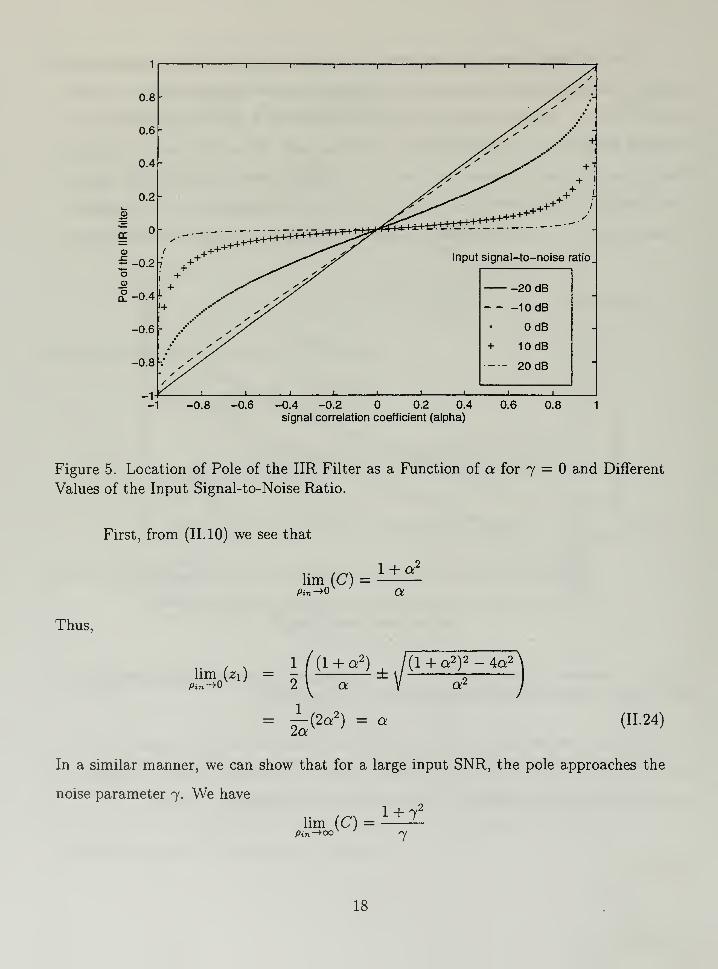
5. Location of Pole of the IIR Filter as a Function of a for 7 = and Different
Values of the Input Signal-to-Noise Ratio 18
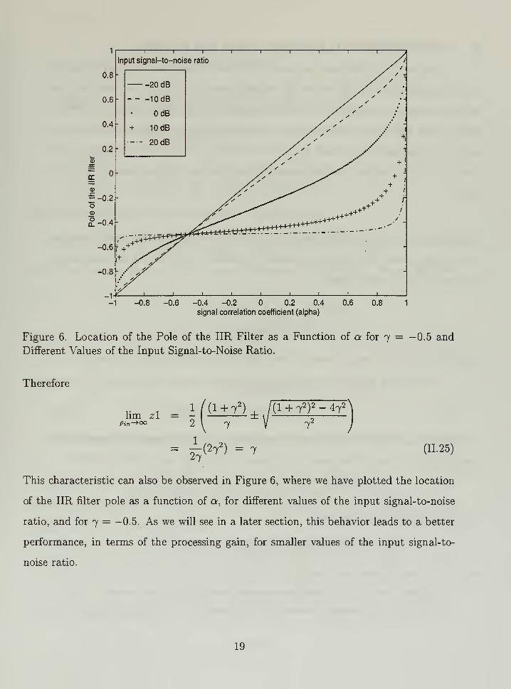
6. Location of the Pole of the IIR Filter as a Function of a for 7 = —0.5 and
Different Values of the Input Signal-to-Noise Ratio 19
7. Comparison between Theoretical and Experimental Values of Processing
Gain for the IIR Wiener Filter as a Function of a, for 7 = (White Noise)
and Input Signal-to-Noise Ratio dB 22
8. Comparison between Theoretical and Experimental Values of Processing
Gain for the IIR Wiener Filter as a Function of a, for 7 = —0.5 and Input
Signal-to-Noise Ratio -10 dB 23
9. Processing Gain for the IIR Wiener Filter as a Function of a for 7 = and
Different Values of Input Signal-to-Noise Ratio. 24
10. Processing Gain for the IIR Wiener Filter as a Function of a for 7 = —0.5
and Different Values of Input Signal-to-Noise Ratio 25
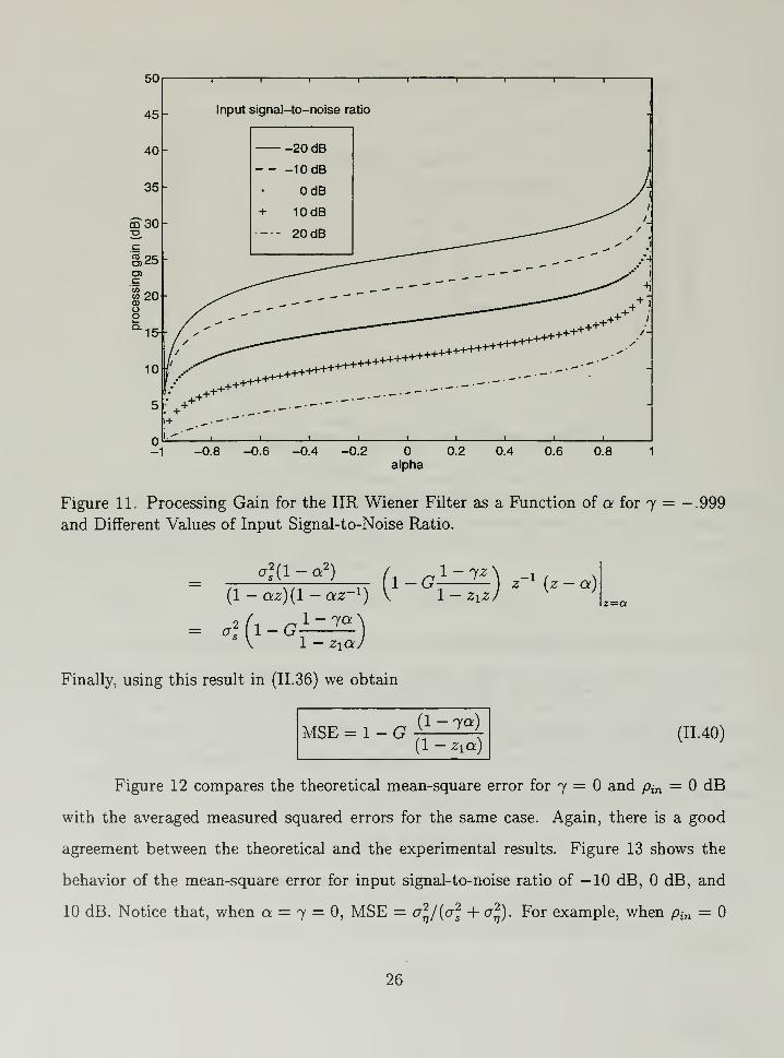
11. Processing Gain for the IIR Wiener Filter as a Function of a for 7 = —.999
and Different Values of Input Signal-to-Noise Ratio 26
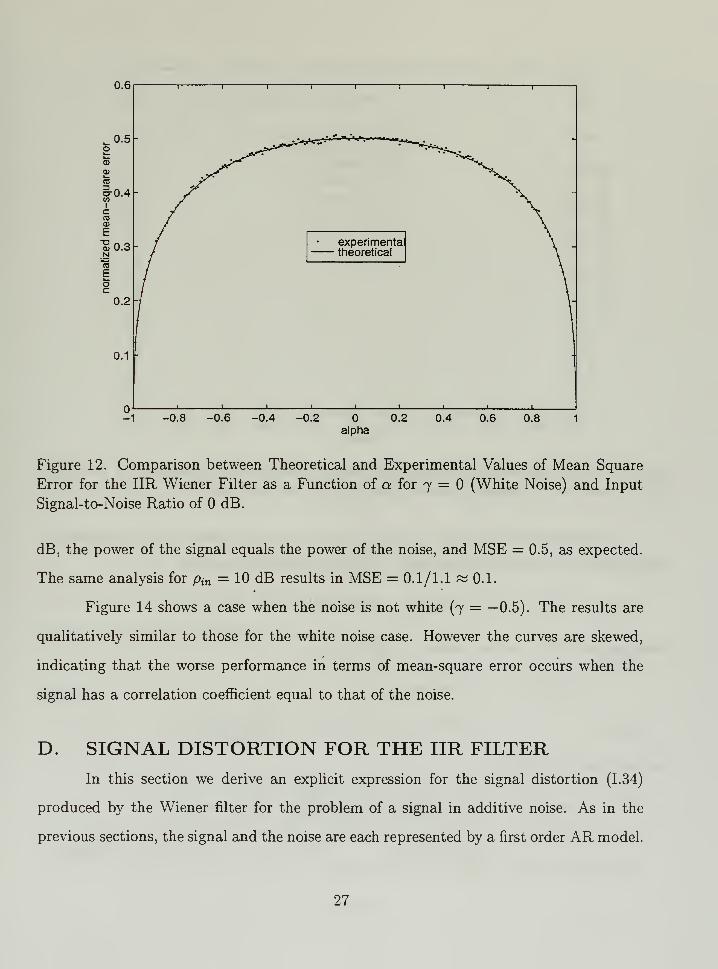
12. Comparison between Theoretical and Experimental Values of Mean Square
Error for the IIR Wiener Filter as a Function of a for 7 = (White Noise)
and Input Signal-to-Noise Ratio of dB 27
IX
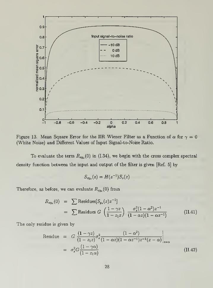
13. Mean Square Error for the IIR Wiener Filter as a Function of a for 7 =
(White Noise) and Different Values of Input Signal-to-Noise Ratio 28
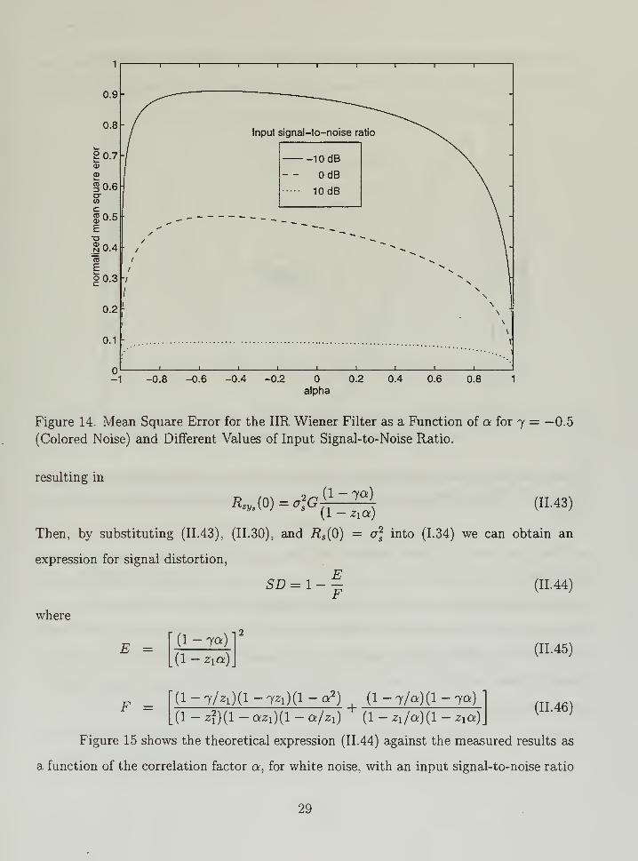
14. Mean Square Error for the IIR Wiener Filter as a Function of a for 7 =
—0.5 (Colored Noise) and Different Values of Input Signal-to-Noise Ratio. . 29
15. Comparison between Theoretical and Experimental Values of Signal Dis-
tortion for the IIR Wiener Filter as a Function of a for 7 = and Input
Signal-to-Noise Ratio dB 30
16. Signal Distortion for the IIR Wiener Filter as a Function of a for 7 =
(White Noise) and Different Values of Input Signal-to-Noise Ratio 31
17. Signal Distortion for the IIR Wiener Filter as a Function of a for 7 = —0.5
(Colored Noise) and Different Values of Input Signal-to-Noise Ratio 32
18. Location of the Zero of the First Order FIR as a Function of the Signal and
Noise Correlation Coefficients {a and 7) for Input Signal-to-Noise Ratio of
dB 37
19. Location of the Zero of the First Order FIR as a Function of the Signal and
Noise Correlation Coefficients (a and 7) for Input Signal-to-Noise Ratio of
-10 dB 38
20. Location of the Zero of the First Order FIR Filter as a Function of a for
7 = —0.5, and for Different Values of the Input Signal-to-Noise Ratio. ... 39
21. Comparison between the Theoretical and Experimental Values of the Pro-
cessing Gain for the First Order FIR Filter for 7 = (White Noise) and
Input Signal-to-Noise Ratio (pin ) of dB 40
22. Comparison between the Theoretical and Experimental Values of the Pro-
cessing Gain for the First Order FIR Filter for 7 = 0.5 (Colored Noise)
and Input Signal-to-Noise Ratio (pin ) of — 10 dB 41
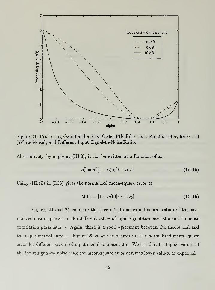
23. Processing Gain for the First Order FIR Filter as a Function of a, for 7 =
(White Noise), and Different Input Signal-to-Noise Ratio 42
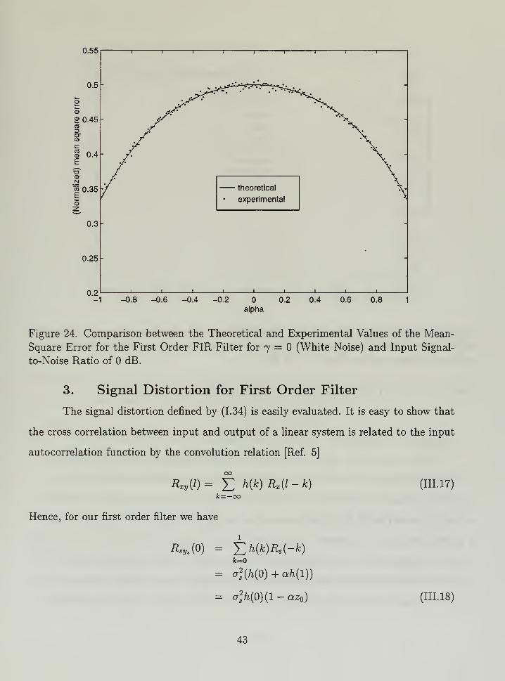
24. Comparison between the Theoretical and Experimental Values of the Mean-
Square Error for the First Order FIR Filter for 7 = (White Noise) and
Input Signal-to-Noise Ratio of dB 43
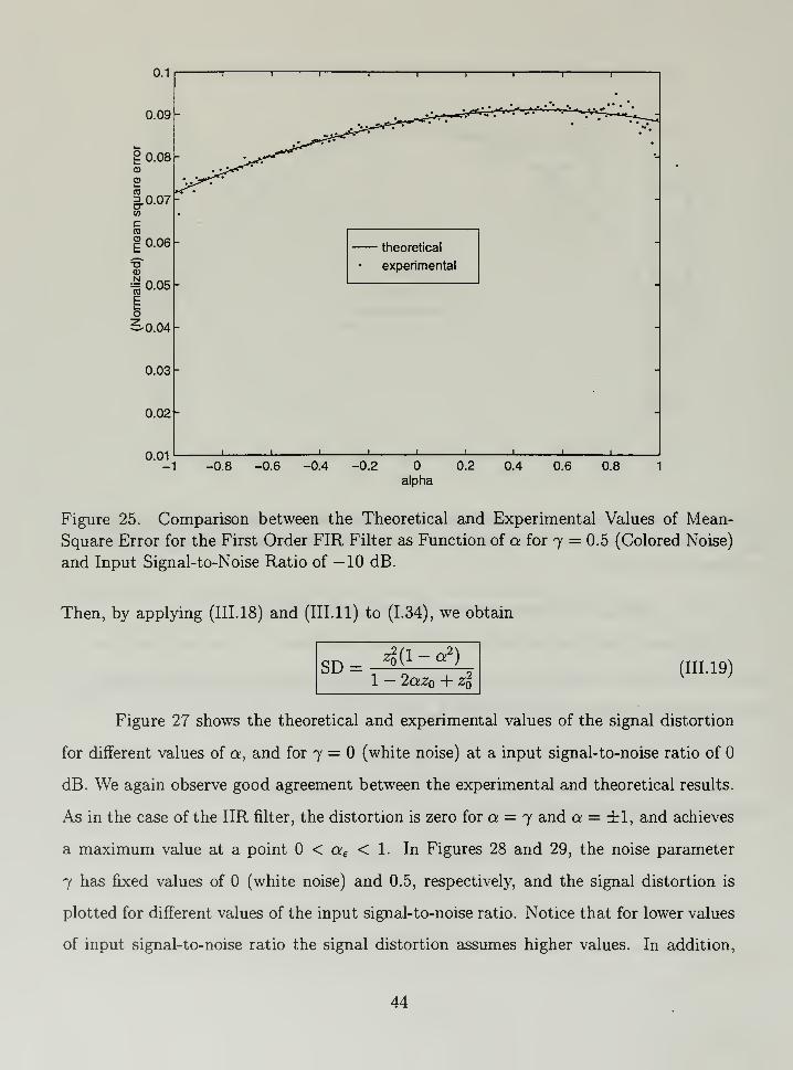
25. Comparison between the Theoretical and Experimental Values of Mean-
Square Error for the First Order FIR Filter as Function of a for 7 = 0.5
(Colored Noise) and Input Signal-to-Noise Ratio of — 10 dB 44
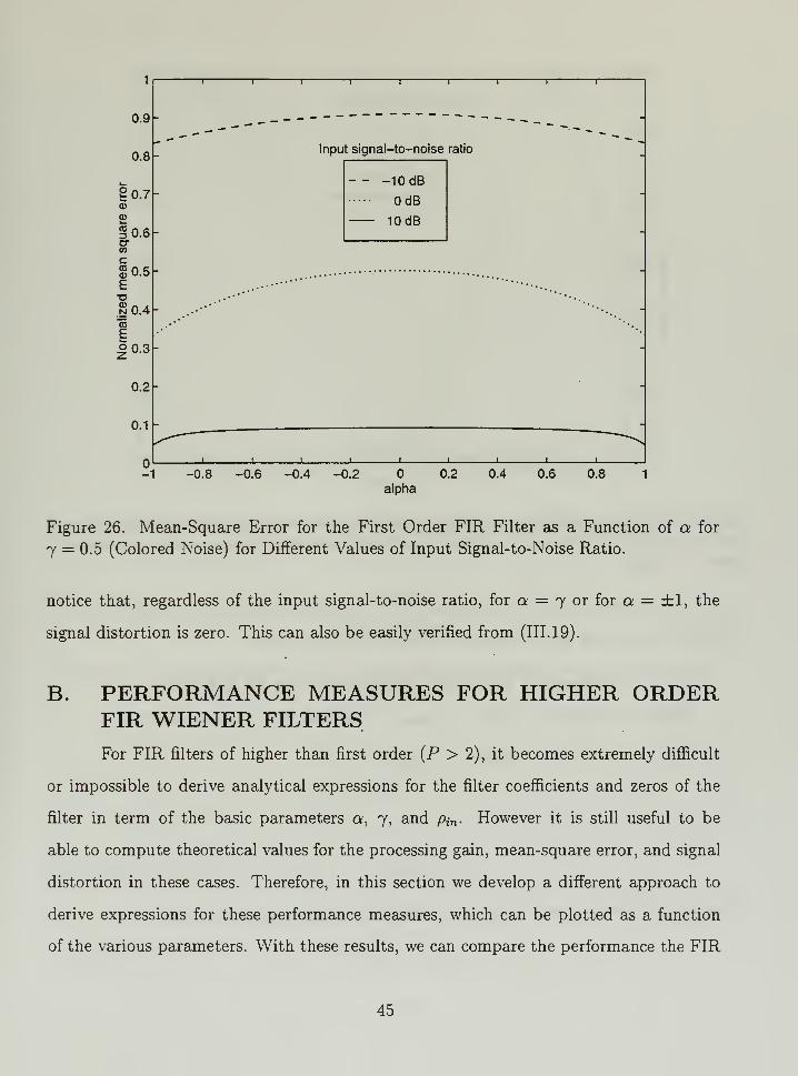
26. Mean-Square Error for the First Order FIR Filter as a Function of a for
7 = 0.5 (Colored Noise) for Different Values of Input Signal-to-Noise Ratio. 45
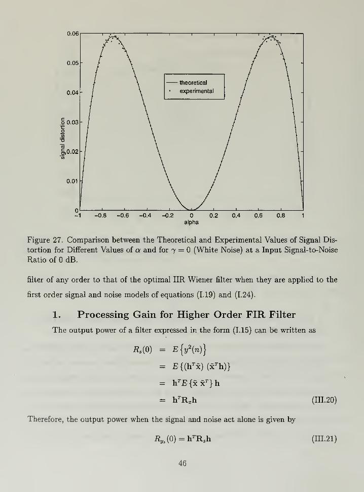
27. Comparison between the Theoretical and Experimental Values of Signal
Distortion for Different Values of a and for 7 = (White Noise) at a Input
Signal-to-Noise Ratio of dB 46
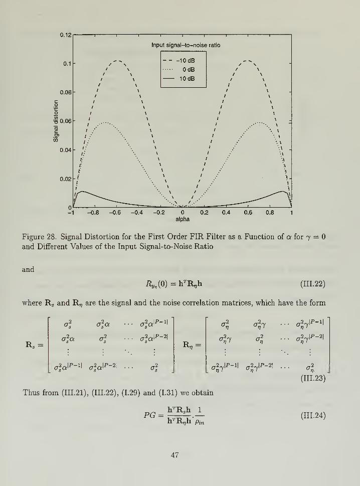
28. Signal Distortion for the First Order FIR Filter as a Function of a for
7 = and Different Values of the Input Signal-to-Noise Ratio 47
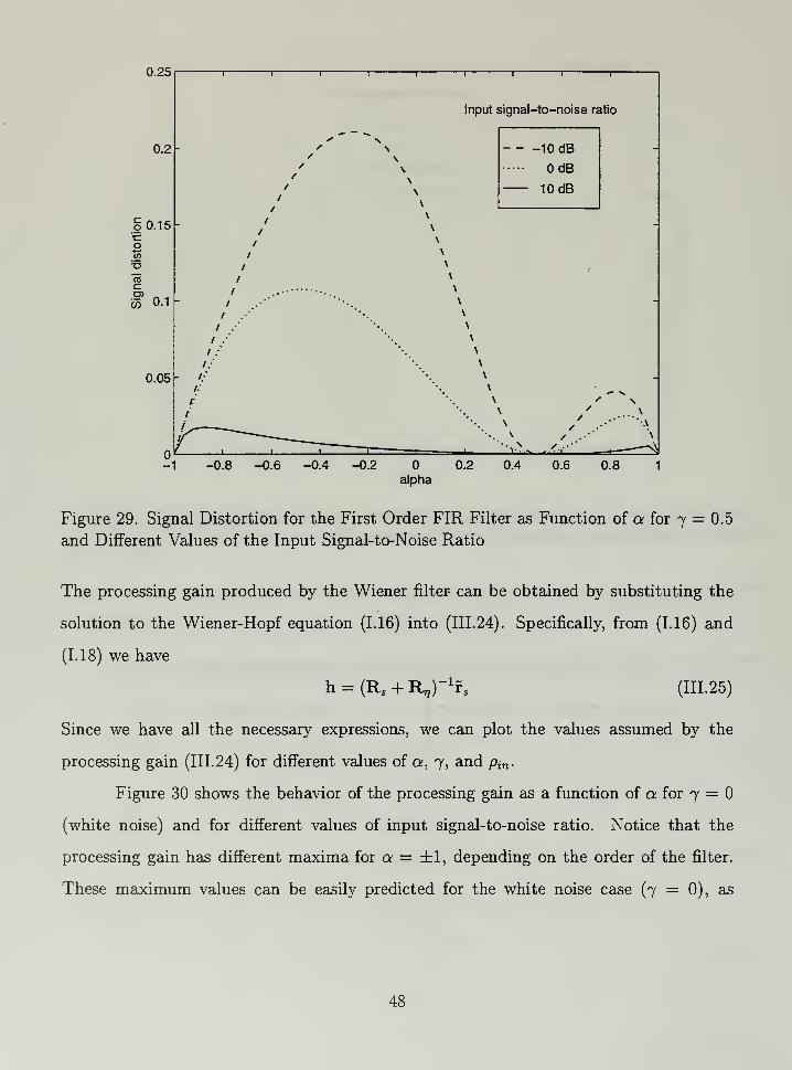
29. Signal Distortion for the First Order FIR Filter as Function of a for 7 = 0.5
and Different Values of the Input Signal-to-Noise Ratio 48
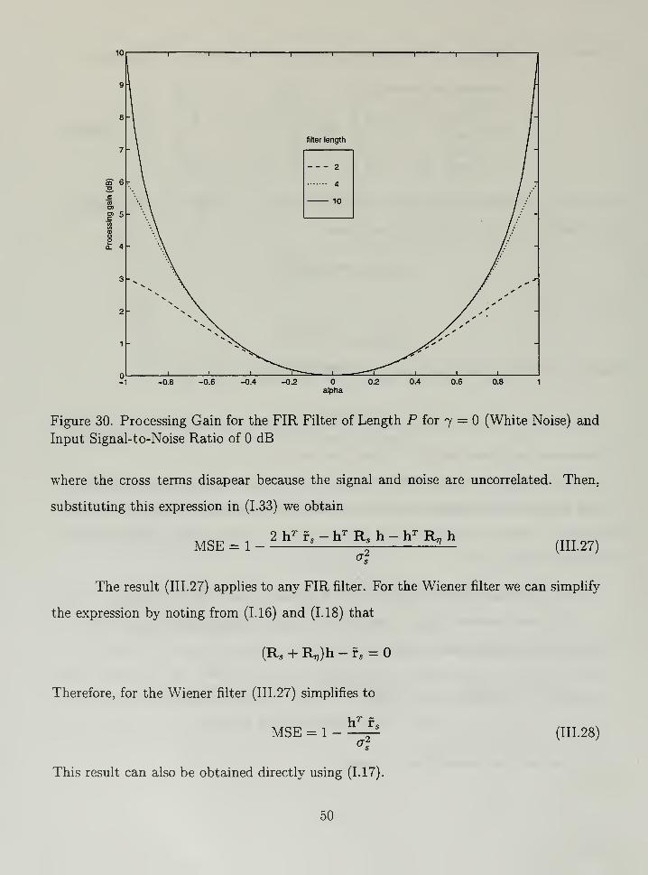
30. Processing Gain for the FIR Filter of Length P for 7 = (White Noise)
and Input Signal-to-Noise Ratio of dB 50
31. Mean-Square Error for the FIR Filter of Length P for 7 = (White Noise)
and Input Signal-to-Noise Ratio of dB 51
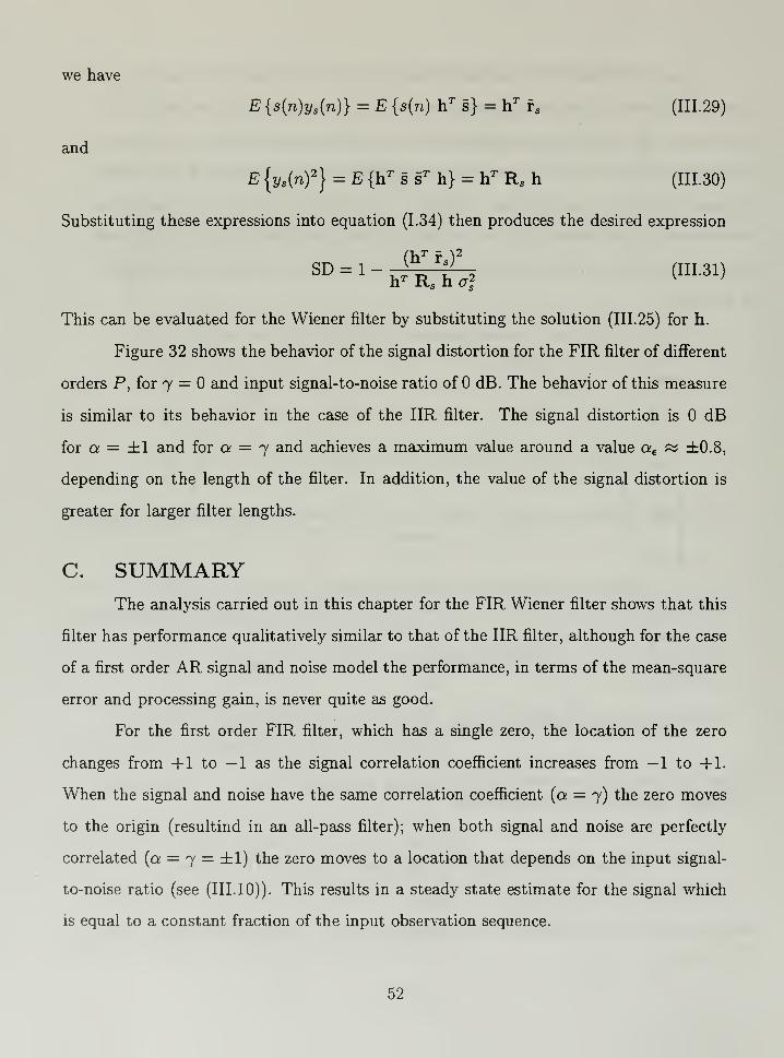
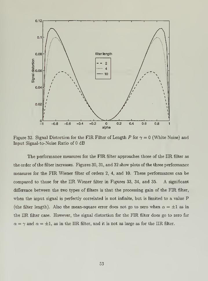
32. Signal Distortion for the FIR Filter of Length P for 7 = (White Noise)
and Input Signal-to-Noise Ratio of dB 53
33. Processing Gain for the IIR Filter for 7 = (White Noise) and Input
Signal-to-Noise Ratio of dB 54
34. Normalized Mean-Square Error for the IIR Filter for 7 = (White Noise)
and Input Signal-to-Noise Ratio of dB 55
35. Signal Distortion for the IIR Filter for 7 = (White Noise) and Input
Signal-to-Noise Ratio of dB 56
xi
36. Processing Gain for the Generalized Wiener Filter as Function of a and A
for 7 = (White Noise) and Input Signal-to-Noise Ratio of dB 60
37. Mean-Square Error for the Generalized Wiener Filter as Function of a and
A for 7 = (White Noise) and Input Signal-to-Noise Ratio of dB .... 61
38. Signal Distortion for the Generalized Wiener Filter as Function of a and
A for 7 = (White Noise) and Input Signal-to-Noise Ratio of dB 62
39. Prewhitening in Short-Time Extended Filtering Algorithm. 64
40. Overlap Averaging Technique Used in Noise Removal 65
41. Results of the Application of the Extended Optimal Filtering Technique
to a Synthetically Generated Short Pulse Signal with Added Low Power
White Noise, for Minimum Residual Noise (A = 1). (a) Original Clean
Data, (b) Original Data plus White Noise, (c) Processed Data 68
42. Results of the Application of the Extended Optimal Filtering Technique
to a Synthetically Generated Short Pulse Signal with Added Low Power
White Noise, for Residual Noise Power Equivalent to 30% of the Input
Noise Power, (a) Original Clean Data, (b) Original Data plus White
Noise, (c) Processed Data (d) Values of A for Each Segment 69
43. Results of the Application of the Extended Optimal Filtering Technique
to a Synthetically Generated Short Pulse Signal with Added Low Power
White Noise, for Residual Noise Power Equivalent to 70% of the Input
Noise Power, (a) Original Clean Data, (b) Original Data plus White
Noise, (c) Processed Data (d) Values of A for Each Segment 70
44. Results of the Application of the Extended Optimal Filtering Technique
to a Killer Whale Song for Minimum Residual Noise (A = 1). (a) Original
Noisy Data, (b) Processed Data 71
45. Results of the Application of the Extended Optimal Filtering Technique
to a Killer Whale Song for Residual Noise Power Equivalent to 20% of the
Input Noise Power, (a) Original Noisy Data, (b) Processed Data 72
xn
ACKNOWLEDGMENTS
The author thanks Father in Heaven for all the bestowed blessings that made this
work possible.
Thanks to my wife, Cristiane, and my daughters, Beatriz and Fernanda, for the
love, patience and support. Without them, there would not be much motivation to
accomplish such challenging task.
Also, thanks to Professor Charles W. Therrien for his support and encouragement
during all the research process.
Xlll
XIV
I. INTRODUCTION
A. MOTIVATION FOR THE STUDYData from passive sonar is generally accompanied by ambient noise arising from
shipping traffic, marine life, wave motion, moving or cracking ice (in the Arctic and
Antarctic), and numerous other sources. The statistical properties of the noise are vari-
able, even direction-dependent, and have been the source of many studies and analyses
[Refs. 1, 2, and 3]. Noise degrades sonar data collection and related processing of the
data to extract information.
Since ambient noise cannot be completely avoided when collecting real underwa-
ter acoustic data, it is desired, in many situations, to remove the noise before further
processing. In general, the signals of interest and the ambient noise are non-stationary
and their statistics are not known a priori. Here we approach the problem of removing
additive noise from a given signal by using a short-time optimal filtering technique. In
this approach we assume that the noise is stationary for the duration of the signal, and
that the signal can be assumed stationary over very short time intervals. We exploit this
feature and develop improved algorithms for removing the noise.
The work in this thesis basically consists of two parts. In the first part (Chapters
II and III), we perform a detailed analysis of the Wiener filter and evaluate its perfor-
mance using three different criteria. For this work we use a simple signal model which
nevertheless provides insight into results for more general types of signals. Both the IIR
and FIR forms of the filter are considered. In the second part (Chapters IV and V), we
propose a new algorithm based on a generalization of the Wiener filter and motivated by
our analysis, that can be applied to real data. The implementation of the algorithm on a
short-time basis is similar to that developed by Frack [Ref. 4] and we use the same basic
structure of the programs. Results of the application of this algorithm to underwater
acoustic data (biologic data) are presented.
B. PROBLEM DESCRIPTIONIn this section we describe the problem of noise removal to be addressed and
introduce the Infinite Impulse Response (IIR) and the Finite Impulse Response (FIR)
forms of the Wiener filter used to estimate the signal in noise.
1. Problem Statement
We consider here the problem of estimating a signal in additive noise. The ob-
served discrete observation sequence is given by
x(n) = s(n) + r)(n) (1.1)
where s(n) is the signal and 77(71) is the noise. The signal duration may be anywhere
from a few miliseconds to a few seconds and is generally a nonstationary random process.
The noise is assumed to be stationary over the entire observation interval and may be
observed without the signal during the early part of the observation interval. That is,
the signal becomes non-zero some time after the beginning of the observation interval,
and the precise time at which it becomes non-zero is not known. Statistics for the signal
and noise, such as mean or correlation function, are not known a priori and must be
estimated from the data.
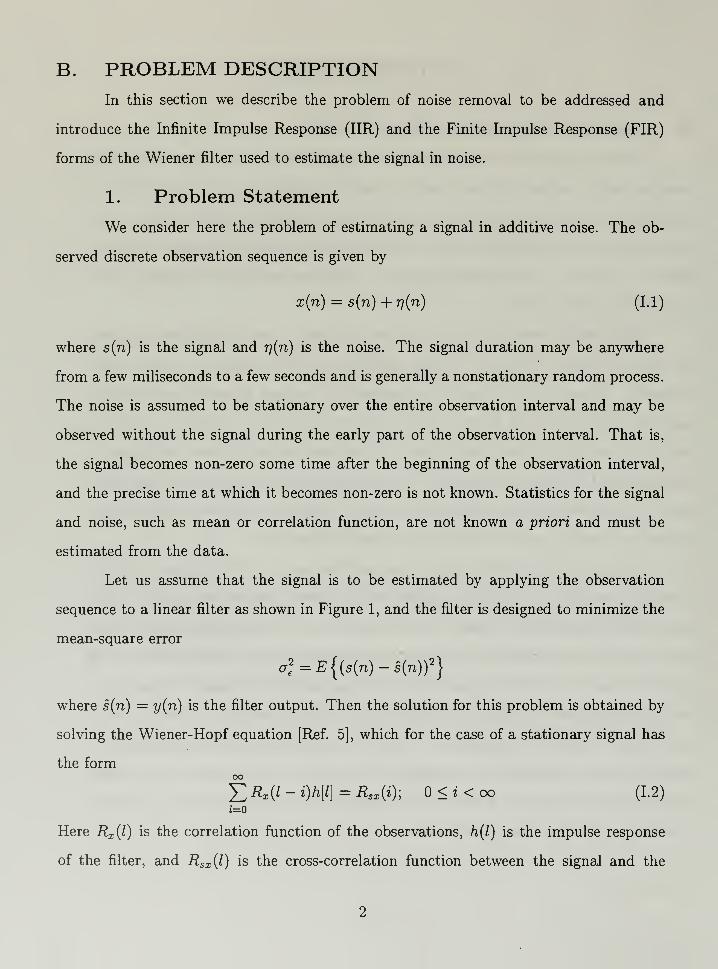
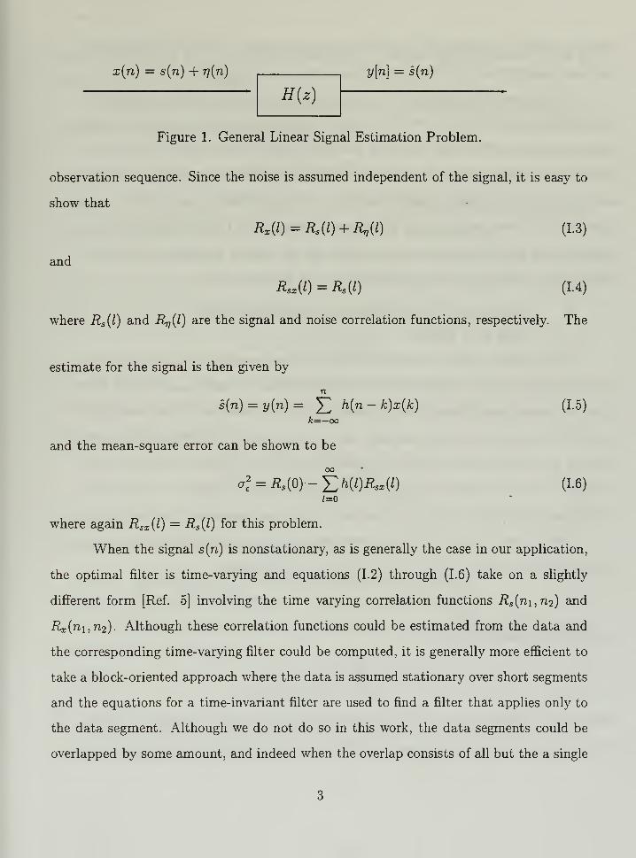
Let us assume that the signal is to be estimated by applying the observation
sequence to a linear filter as shown in Figure 1, and the filter is designed to minimize the
mean-square error
o\ = E {(s(n) - s(n))2
}
where s(n) = y(n) is the filter output. Then the solution for this problem is obtained by
solving the Wiener-Hopf equation [Ref. 5], which for the case of a stationary signal has
the form00
Y, RX {1 - i)h[l] = Rsx (i)\ < i < 00 (1.2)
1=0
Here Rx (l) is the correlation function of the observations, h(l) is the impulse response
of the filter, and Rsx (l) is the cross-correlation function between the signal and the
H{z)
y[n] = s(n)x(n) = s(n) + r](n)
Figure 1. General Linear Signal Estimation Problem.
observation sequence. Since the noise is assumed independent of the signal, it is easy to
show that
Rx(l) = Rs{l) + Rv(l) (1.3)
and
Rsx (l) = Rs (l) (1-4)
where Rs (l) and Rq{l) are the signal and noise correlation functions, respectively. The
estimate for the signal is then given by
n
s(n) = y(n)= ]£ h{n - k)x{k) (1.5)
k=— oo
and the mean-square error can be shown to be
oo
a2
e=Rs(0)- Y, h(l)Rsx {l) (1.6)
1=0
where again RSX {1) — Rs(l) for this problem.
When the signal s(n) is nonstationary, as is generally the case in our application,
the optimal filter is time-varying and equations (1.2) through (1.6) take on a slightly
different form [Ref. 5] involving the time varying correlation functions Rs (ni,ri2) and
Rx (ni,n2 ). Although these correlation functions could be estimated from the data and
the corresponding time-varying filter could be computed, it is generally more efficient to
take a block-oriented approach where the data is assumed stationary over short segments
and the equations for a time-invariant filter are used to find a filter that applies only to
the data segment. Although we do not do so in this work, the data segments could be
overlapped by some amount, and indeed when the overlap consists of all but the a single
point, the result is equivalent to using the time-varying filter. Thus for purposes of our
work and analysis here, (1.2) through (1.6) are the relevant equations.
The Wiener-Hopf equation (1.5) can be solved for two types of filters, the Infinite
Impulse Response (IIR) filter, which is applied recursively to the data, and the Finite
Impulse Response (FIR) filter, where the filtering process involves a simple convolution.
Both of these filters are known as Wiener optimal filters and are described in following
sections. Later, we investigate the performance of these two filters in the case when both
signal and noise are represented by a first order autoregressive (AR) model. This inves-
tigation using a simple model provides insight into the general behavior of the Wiener
Filter, and so, helps to predict its behavior for more involved cases.
2. Solution of The Wiener-Hopf Equations:
The IIR Filter
The IIR Wiener filter is recursive in form and can have the advantage of requiring
fewer parameters than a comparable FIR form of the filter. In many cases the IIR filter
is the only true optimal solution to the problem and FIR filters are in fact suboptimal
since they do not achieve the absolutely lowest mean-square error. Since the filter is
required to be causal, the problem is not straightforward; it was solved (originally in the
continuous case) by Wiener using spectral factorization methods [Ref. 6]. Because the
solution procedure will be referred to later in this work, we summarize it in this section.
The solution for the IIR filter derives from observing that if the observation se-
quence is a white noise process Rx (l) = Oq5{1) then (1.2) becomes
CO
J2^oS(l-i)h{l) = Rsx {i); < % < oo (1.7)
;=o
leading to the simple solution
h(l) = \n sxK > ~ (1.8)
I <0
The procedure then is to first whiten the observed random process x and then apply the
solution above. Thus we conceptually represent the optimal filter /iasa cascade of two
filters, the whitening filter g, and the optimal filter ti for the whitened process. Both g
and ti are required to be causal.
To find the whitening process we observe [Ref. 5] that the complex spectral density
function of the input process x can be factored as
Sx (z) = /CoHca (z)Hca (z ) (1.9)
Therefore, if we choose G(z) = l/Hca {z), we see that the filter g will have the necessary
whitening properties and the whitened input process will have variance Kq.
The cross-correlation between the whitened input process and the signal has a
complex cross-spectral density function given by Ssx {z)/Hca {z~l)\ therefore, the filter
corresponding to (1.8) for the whitened process is written as
A-0
Ssx(z)
HCa(z-l)(1.10)
where the notation[ ]+ means that the resulting function corresponds only to the causal
part of the quantity within brackets. Finally, by cascading G(z) and H (z) we obtain the
expression for the optimal IIR filter
H(z) =1
JCoHca (z)
Ssx(z)
[Hca(z-i)
(1.11)
where Hca (z) and Kq are derived from the spectral factorization (1.9), and Ssx (z) is the
cross spectral density function for s(n) and x(n).
3. Solution of The Wiener-Hopf Equations:
The FIR Filter
The FIR filter is simpler to derive. Since the filter has finite length P, the filtering
equation (1.5) can be written as
p-i
y(n) = ]C K l)x
(n -
1=0
(1.12)
We can also directly apply (1.2) noting that the upper and lower limits need to reflect
the causality and finite length of the filter. The Wiener-Hopf equation for real process
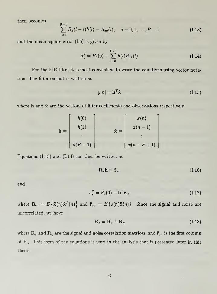
then becomesp-i
Y,Rx{l~ i)h{l) = Rsx (i); i = 0, 1, . ..
,
P - 1 (1.13)
1=0
and the mean-square error (1.6) is given by
p-i
a\ = Rs (0) - J2 h(l)Rtx (l)
1=0
(1.14)
For the FIR filter it is most convenient to write the equations using vector nota-
tion. The filter output is written as
y[n] = hJ x
where h and x are the vectors of filter coefficients and observations respectively
(1.15)
h =
MO)
Mi)X =
x{n)
x(n — 1)
h(P-l) x(n-P + l)
Equations (1.13) and (1.14) can then be written as
Rxh = rsx (1.16)
and
g\ = Rs (0) - hTrsx (1.17)
where Rx = EJx(n)xT (n)| and fsx = E {s(n)5t(n)}. Since the signal and noise are
uncorrelated, we have
R^Ra + R, (1.18)
where Rs and R^ are the signal and noise correlation matrices, and rsx is the first column
of Rs . This form of the equations is used in the analysis that is presented later in this
thesis.
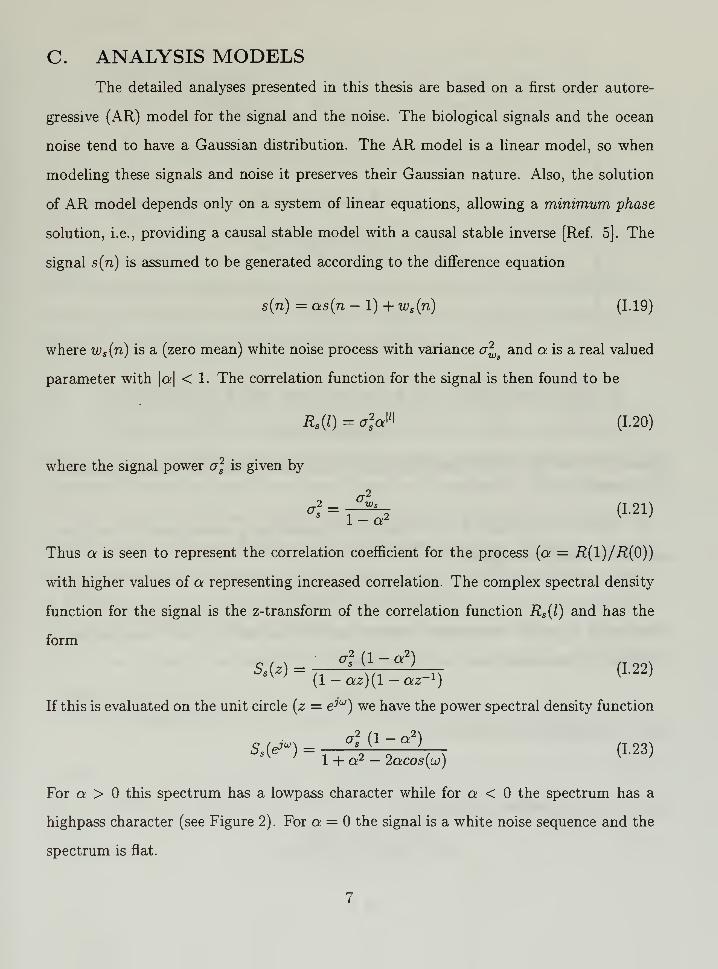
C. ANALYSIS MODELSThe detailed analyses presented in this thesis are based on a first order autore-
gressive (AR) model for the signal and the noise. The biological signals and the ocean
noise tend to have a Gaussian distribution. The AR model is a linear model, so when
modeling these signals and noise it preserves their Gaussian nature. Also, the solution
of AR model depends only on a system of linear equations, allowing a minimum phase
solution, i.e., providing a causal stable model with a causal stable inverse [Ref. 5]. The
signal s(n) is assumed to be generated according to the difference equation
s(n) = as(n — 1) 4- ws (n) (1-19)
where ws (n) is a (zero mean) white noise process with variance a^sand a is a real valued
parameter with \a\ < 1. The correlation function for the signal is then found to be
R,(l) = a2aw (1.20)
where the signal power a2is given by
a.2
1 — or
Thus a is seen to represent the correlation coefficient for the process (a — R(1)/R(0))
with higher values of a representing increased correlation. The complex spectral density
function for the signal is the z-transform of the correlation function Rs (l) and has the
form
S.W =,,
a2A\;
a2)
n (1.22)v ; (l-az)(l -az~ l)
K'
If this is evaluated on the unit circle (z = eJW ) we have the power spectral density function
a2(1 - a2
)
v' 1 + a2 - 2acos{u)
y J
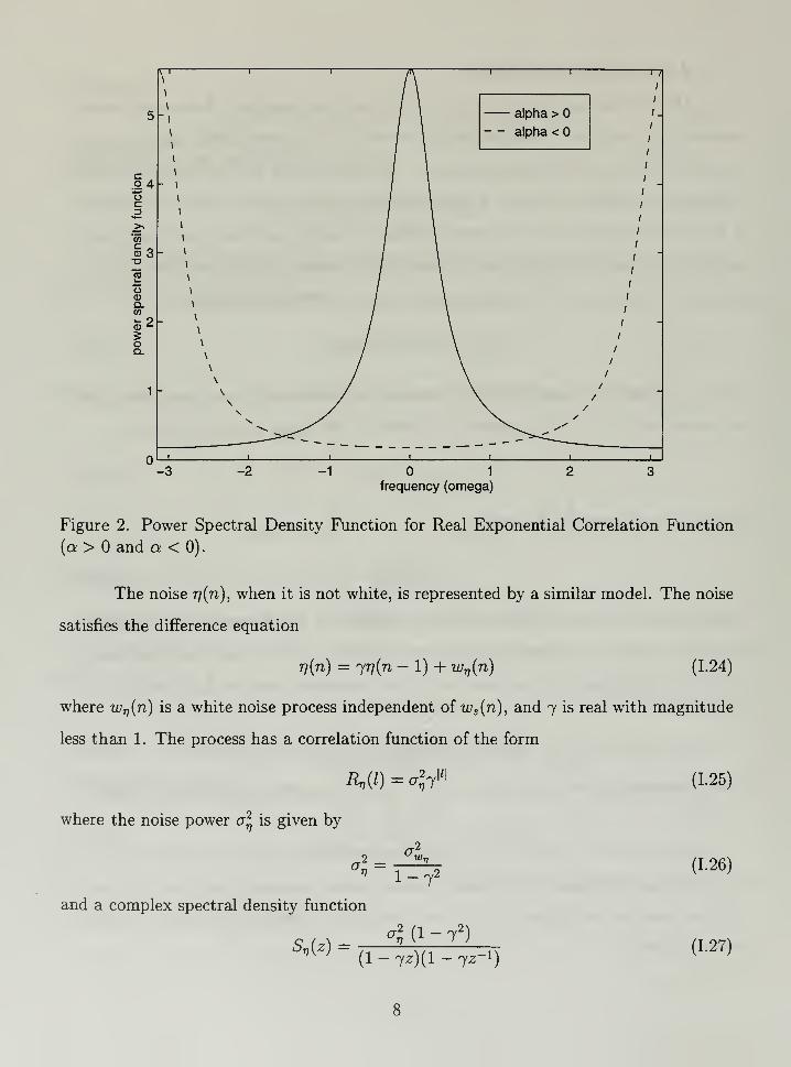
For a > this spectrum has a lowpass character while for a < the spectrum has a
highpass character (see Figure 2). For a = the signal is a white noise sequence and the
spectrum is flat.
alpha >— alpha <
|4oc3
i
i
i
.
-3 -2 -1 1
frequency (omega)
Figure 2. Power Spectral Density Function for Real Exponential Correlation Function
(a > and a < 0).
The noise rj(n), when it is not white, is represented by a similar model. The noise
satisfies the difference equation
r)(n) = 777(72 - 1) + wv (n) (1.24)
where wv (n) is a white noise process independent of ws (n), and 7 is real with magnitude
less than 1. The process has a correlation function of the form
RnQ) = °2y i
(L25
)
where the noise power a* is given by
a2.
(1.26).2 *«,n !_ 7
2
and a complex spectral density function
ol (1 - 72)
i" (Z'-(l- 7z)(l-7Z- 1
)
(1.27)
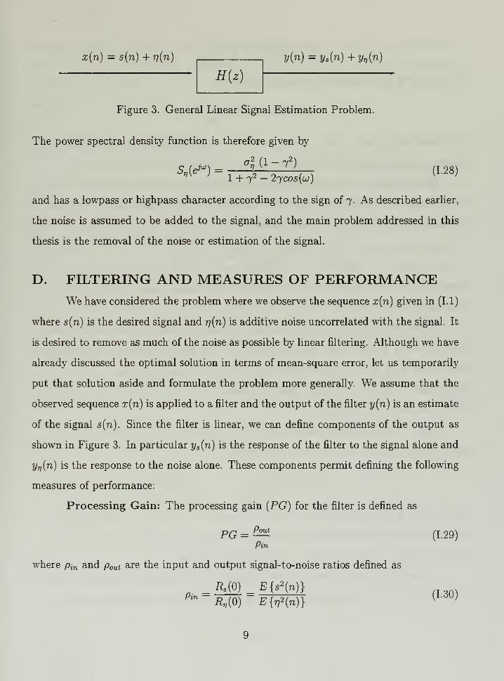
H(z)
y(n) = ys (n) + yv {n)x(n) = s(n) + 77(71)
Figure 3. General Linear Signal Estimation Problem.
The power spectral density function is therefore given by
<W) = 1
—
V o \ ^ (L28
)
and has a lowpass or highpass character according to the sign of 7. As described earlier,
the noise is assumed to be added to the signal, and the main problem addressed in this
thesis is the removal of the noise or estimation of the signal.
D. FILTERING AND MEASURES OF PERFORMANCEWe have considered the problem where we observe the sequence x(n) given in (1.1)
where s(n) is the desired signal and 77(72) is additive noise uncorrelated with the signal. It
is desired to remove as much of the noise as possible by linear filtering. Although we have
already discussed the optimal solution in terms of mean-square error, let us temporarily
put that solution aside and formulate the problem more generally. We assume that the
observed sequence x(ri) is applied to a filter and the output of the filter y(n) is an estimate
of the signal s(n). Since the filter is linear, we can define components of the output as
shown in Figure 3. In particular ys {n) is the response of the filter to the signal alone and
yv {n) is the response to the noise alone. These components permit defining the following
measures of performance:
Processing Gain: The processing gain (PG) for the filter is defined as
Pin
where pin and pout are the input and output signal-to-noise ratios defined as
RM E{s2(n)}
Pinfi,(0) EW{n)}
(1.30)
RyM __ E{y*(n)}Pmt ~ R,M~ E{y^n)}
(U1)
The processing gain is usually measured in dB, i.e.,
PG(dB) = 101og10^ (1.32)Pin
Processing gain relates to the relative power in the signal and the noise but does not
address accuracy of the signal estimate.
Mean Square Error: The mean-square error is the estimated value of the
squared difference between the signal and the filtered output. Here we use a normal-
ized measure of the mean-square error defined by
MSE =E{(g)-y } = |M
E{s2 {n)} R8 (0)
where Re (l) is the correlation function for the "error" defined as e(n) = s(n) — s(n) =
s(n) - y(n).
When the output of the filter is equal to the signal itself (except possibly at a
countable set of points) then the mean-square error is equal to zero. The maximum
occurs when y(n) is zero, where this normalized mean-square error has a value of 1.
Mean-square error is the quantity that is optimized in the traditional Wiener optimal
filtering problem discussed above.
Signal Distortion: Signal distortion (SD) addresses what the filter does to the
signal itself irrespective of the noise, and is defined as
qn _ , _ E{s(n)ys (n)}2
_ , _ KM „ „,E {«*(„)} E{j,2(„)} Rs{0)Ry,(0)
{'
where Rsys {l) is the cross-correlation function between s(n) and ys (n). This quantity
takes on values in the interval [0, 1] and is minimized when the signal is unchanged by
the filter (ys {n) = s(n)), i.e., there is no distortion introduced.
An ideal filter would form a perfect estimate for the signal and completely elimi-
nate the noise. Such a filter would have infinite processing gain, zero mean-square error,
10
and zero signal distortion. Since no linear filter can achieve such ideal performance,
we can balance these measures, depending on the application, emphasizing one measure
compared to the others. Thus all of the measures denned above will have use in the
sequel.
E. THESIS OUTLINEThe remainder of this thesis is organized as follows. Chapter II introduces, anal-
yses and discusses the performance of the IIR Wiener filter described above. Chapter
III provides a similar analysis and discussion of the performance for the FIR form of
the Wiener filter. Chapter IV presents a filter based on a new criterion that serves as a
generalization of the FIR Wiener filter. This filter, which we call the extended optimal
filter, provides a way to improve the signal distortion with only slight degradation in the
other performance measures. Chapter V incorporates this technique in a noise removal
algorithm based on short term filtering of the observation sequence and demonstrates
its performance on sonar data. Chapter VI concludes the thesis with a summary and
suggestions for further investigation.
11
12
II. ANALYSIS OF THE IIR WIENER FILTER
In this chapter we derive analytical expressions for the Wiener IIR optimal filter
for a signal in colored noise. The signal and the noise are each represented by a first
order AR model (equations (1.19) and (1.24)). The expressions for the filter generalize
the results obtained in [Ref. 5] which treats the white noise case only.
After deriving an expression for the optimal filter we derive the corresponding
expressions for the measures of performance outlined in Chapter I and examine these
expressions as a function of some of the parameters describing the model. While the
model expressed by (1.19) and (1.24) is only of first order, it exhibits many of the gen-
eral characteristics of a more complicated model and allows us to draw several general
conclusions.
A. THE IIR WIENER FILTER
The general expression for the optimal IIR (Wiener) filter for estimating a real-
valued signal s(n) in additive noise rj[n] (see (1.1)) is given by equation (1. 11). For the
case of a first order AR model, the signal and noise complex spectral density functions
are given by (1.22) and (1.27) respectively. Since the signal and noise are independent
with zero mean, it follows from (1.4) that the complex spectral density function between
the signal s(n) and the observation x(n) is given by
^' =^°Ffe (IL1)
Similarly, it follows from (1.3) that the complex spectral density function for the obser-
vations is
Sx (z) = Ss (z) + Sv (z)
trjfl-a2) ^2(l-72
)
(1 -az)(l -az~ l
) (1 -jz)(l -yz~ l
)
a2s{l - |a|
2)(l + 7
2 - jz - jz' 1
) + a2(l - |t|
2)(1 + a2 - az - az~ l
)
(1 - az~ l ){l - az)(l - 7^- 1 )(l - jz)
13
By collecting terms, this last equation can be written as
-Az + B- Az~ l
where
Sx (z) =D(z)
(II.2)
A = 7a2(l-a2
) + a<72 (l- 7
2) (II.3)
B = a2(l-a2)(l + 7
2) + ^(l-72
)(l + a2)
(II.4)
and
D(z) = {1- az~ l){l - az)(l - 72
_1)(1 - 72)
After factoring the numerator, we can write (II. 2) as
—Az-1
Sx(z) = —R7ZT (Z ~ Zla)(z ~ z\b)
D(z)
where
Zlb = l(c + Vc^a)
and
c _ B _ a2(l ~ *2
)(1 + 72) f <#1 ~ 7
2)(1 + a2
)
' A~
0-2(1 - a2)7 + cr2(l -j2)a
This last constant can be expressed as a function of a, 7, and pin , as
C = [An (l-o:2)(l + 7
2)/(l-72)] + (l+tt2
)
[pm7(l-a2)/(l- 72)] + a
where pin is the input signal-to-noise ratio
(0.5)
(II.6)
(II.7)
(II.8)
(II.9)
(11.10)
Pin — o (11.11)
14
From the form of the polynomial in (II. 2) and (II.6), it can be seen that ziaZib = 1, or
that zu = l/zia . Let us denote the root that is inside the unit circle in the complex
plane as Zi, i.e.,
lfKI<1(11.12)
zu, = l/zia otherwise
Then from (11.10), we see that Z\ depends only on a, 7, and pin .
We can now factor the complex spectral density function Sx (z) by writing it in
the form
zl=
Sx (z) =(l-zlZ
-i)(1 - zlZ )
zi {1 — az~ l ){l — ^z~ l
) (1 — az)(l — jz)
In comparing this with (1.9) we can identify
/C = A/zi
(11.13)
(11.14)
and
Hca (z) =(l-ziz- 1
)
(1 - az~ l )(l - yz~ l
)
bsx\Z)
Hca(z- 1
) +
Let us now proceed to compute the term
equation for the optimal filter. From (II. 1) and (11.15), we have
Ssx (z) = as
2 (l-la| 2)
(l-a*)(l- 7*)
Hca {z-1
) {1 - az){l - az~ l
) (1 - Zl z)
(11.15)
that appears in (1. 11), the
ziz {l-az~ l)(l- (1/Zl )z-1)
This can be written in a partial fraction expansion as
Ssx {z) C\.
C2+
where
and
»„(*"') (l-az-i) (1 - (1/z,)*" 1
)
Cl = ^ (1 -N 2)
7l - (1M)zx (1 - 1/zia)
ft-oja-MV'1 -
zi (1 - zx a)
(11.16)
(11.17)
(11.18)
15
The causal part of the expression (11.16) can now be written as
H'(z) = i-Hca
(z-i)
Ci
1 — az~ l
Z\ 1-
1-
- 1 /cry
- l/zia
*2(i -- M 2
) llzi
A i — az~ l
Z\ a --l/7 <^ -l«|
2) 7/*
>1 a — 1/^! 1 — az-1
Finally, combining (11.15) and (11.20) we obtain
H(z) =Hca{z) /C
Ssx(z)
Hca{z-l)
(1 - az- l)(l - 7Z" 1
) zx a- l/7 <r5
2(l - \a\
2)j/z,
(1 - ^i*"1
)A a- 1/zi (1 - az_1
)
The final expression for the Wiener optimal IIR filter can thus be written as
where the gain G is given by
G = Z\ QfJ 1 2/11
i2\
A a^i — 1
(11.19)
(11.20)
(ziOZi-Zi/j 2 2\ / l~7g 1
\
(11.22)
(11.23)
It is interesting to note that the filter places a zero at z = 7 in an attempt to cancel the
additive noise. Also, it is important to note that z\ is just a function of the constant C,
and, therefore, through (11.10), it is just a function of the input signal-to-noise ratio pin ,
the signal parameter a, and the noise parameter 7.
16
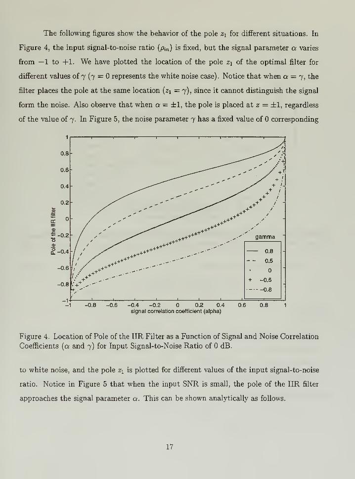
The following figures show the behavior of the pole z\ for different situations. In
Figure 4, the input signal-to-noise ratio (pin ) is fixed, but the signal parameter a varies
from —1 to +1. We have plotted the location of the pole z\ of the optimal filter for
different values of j (7 = represents the white noise case) . Notice that when a = 7, the
filter places the pole at the same location (z\ = 7), since it cannot distinguish the signal
form the noise. Also observe that when a = ±1, the pole is placed at z = ±1, regardless
of the value of 7. In Figure 5, the noise parameter 7 has a fixed value of corresponding
-1
gamma
_i i_ j i_ _i l
0.8
- - 0.5
+ -0.5
-0.8
-0.8 -0.6 -0.4 -0.2 0.2 0.4 0.6
signal correlation coefficient (alpha)
0.8
Figure 4. Location of Pole of the IIR Filter as a Function of Signal and Noise Correlation
Coefficients (a and 7) for Input Signal-to-Noise Ratio of dB.
to white noise, and the pole z x is plotted for different values of the input signal-to-noise
ratio. Notice in Figure 5 that when the input SNR is small, the pole of the IIR filter
approaches the signal parameter a. This can be shown analytically as follows.
17
0.8
0.6
0.4
0.2
-0.2
0.4
0.6
0.8
-1
-11 1 1 r- ! i i i- >
/' •
/'' •'/ 's ' *
/ "/y .'
A' / I/' yi/s jr '
X" ^y' jt^y> / + i
J^ ^"^ +
/
r ++^++++^"H^^5^4-+ _---**^ X
7 ++ ^^'/
Input signal-to-noise ratio.
1 + ^-"^ ^XL+ /^ *7 -20 dB
jr S/1+ / <X - - -10 dBi ••'* '/
OdB -
• //'
s
+ 10 dBS yS_• / jf' ' <S 20 dB• //
> i i i
-1 -0.8 -0.6 -0.4 -0.2 0.2 0.4 0.6 0.8 1
signal con-elation coefficient (alpha)
Figure 5. Location of Pole of the IIR Filter as a Function of a for 7 = and Different
Values of the Input Signal-to-Noise Ratio.
First, from (11.10) we see that
lim (C) = ±±±Pin^o a
Thus,
1 /(1 + a2) 1(1 +
a
2)
2 -4a2
lim (zi) = -I ± '
Pin->0 a a'
2a(2a
2) = a (11.24)
In a similar manner, we can show that for a large input SNR, the pole approaches the
noise parameter 7. We have
1 + 72
lim (C) = -—?-pi„->OO v ry
18
0.8-
0.6
0.4
0.2
03
~ -0.2"o
£a. -'
-0.6
-0.8
-1
I f- T 1— '
Input signal-to-noise ratio
I- - 1 - I ~ - r "' "I -',
/I
-20 dB
- -- -10 dB
OdB
+ 10 dB
- - 20 dB /,'' / +l
-
X-' yS S jr |
^— + '
-
• V."'"
'/-
' "/'
'X
r i i i j 1 1 1 1 1
-1 -0.8 -0.6 -0.4 -0.2 0.2 0.4 0.6 0.8 1
signal correlation coefficient (alpha)
Figure 6. Location of the Pole of the IIR Filter as a Function of a for 7 = —0.5 and
Different Values of the Input Signal-to-Noise Ratio.
Therefore
lim z\1 /(1 + 7
2)
/(l + 72)
2 -472
±7 r
= f (272) = 7
27(11.25)
This characteristic can also be observed in Figure 6, where we have plotted the location
of the IIR filter pole as a function of a, for different values of the input signal-to-noise
ratio, and for 7 = —0.5. As we will see in a later section, this behavior leads to a better
performance, in terms of the processing gain, for smaller values of the input signal-to-
noise ratio.
19
B. PROCESSING GAIN FOR THE IIR FILTER
Using the first order signal and noise model, we can derive an analytical expression
for the processing gain (1.29) for the IIR Wiener Filter. For this we first need the input
and output signal-to-noise ratios. The input signal-to-noise ratio is given by (1.30) or
(11.11), while the output signal-to-noise ratio is given by (1.31). Hence, the problem is
to find expressions for Rys (0) and ^(0) in terms of a, 7, crj, and a*. To do this, first
observe that the complex spectral density of the output of a linear system is given by
[Ref. 5]
Sy(z) = H{z)H{z- l )Sx {z) (11.26)
where H{z) is the filter transfer function and Sx is the complex spectral density function
of the input. Since the correlation function is related to the complex spectral density
function by the inversion formula
Ry(l) = ^-jSy{z)z
l-'dz
= ^Residues[5y (z)z'_1
]
where the residues correspond only to the poles within the unit circle, we have
Ry(0) = ^2Residues[Sy {z)z-1
]
= ^Residues[i7(z)if(z- 1
)5x (z)2"1
](11.27)
To evaluate Rys (0) we use this formula assuming that the input complex spectral density
function Sx (z) is that of the signal. Thus from (11.26), (1.22), and (11.22) we obtain
(11.28)
and, according to (11.27) we have
Rys (0) = RES2=21 + RES2=a + RESZ=0 (11.29)
where the three residues are given by
RFq^(l-T^Xi-T^i-a2
) , ,
52=21 ~(z - Zl )(l - zlZ ){\ - az)(l - az-i) [ lj
Z— Zl
20
RES2=Q —
GV5
2(l-a2)(l- 7Ai)(l-7^i)
{l-z2)(l-a/zl){l-az1 )
G2(l- 7z-')(l- 7z)a2(l-a2
)
(1 - ziz~l){\ - ziz){\ - az)(z - a)
G2a2s(l-7/a)(l-ia)
(1 - Zl/a)(l - ZiCt)
(z-a)
RESz=o —G2(l- 7z-i)(l- 7z)*
2(l-a2)z
z(l - zi^Xl - ziz)(l - az){l - az~ l
)
[Z *l) =2=0
Thus combining these results, we have
(1 - 7/z1 )(l - 720(1 - a2) (1 - 7/a)(l - 7a)
(11.30)(l-zj)(l-a/zi)(l-azi) (l-Va)(l-^aX
In a similar manner we see that the output complex spectral density due to the noise
alone is
c (js 21-yz- 1 l- 7z ^(l-72
)
**,W u•l-2 1
z-i'l-21^'(l- 7z-
1)(l- 7z)
r2 ,T2 (1-72)
'(1 -**-!)(! -**)(11.31)
Applying (11.27) and evaluating the expression at the single pole z — Z\ then leads to
RyM = <G2j^r)
' (n.32)
By taking the ratio of (11.30) and (11.32) we compute the output signal-to-noise
ratio
Pout(l-7M)(l-7*i)
, (1-7A*)(1-70:)(1-*2)
(1 - a/Zl )(l - oan)+
(1 - zi/a)(l - Zl a)(l - a2)
(H '33)
Finally, by substituting (11.11) and (11.33) into the definition (1.29) we obtain the final
expression for the processing gain as
PG = (1 - 77*0(1 - 7*1) (1 - 7/a)(l - 7a)(l - z2)
(1 - a/Zl ){\ - az x ) (1 - Zl /a){l ~ zi*)(l ~ *2)
a
i-r (11.34)
Figure 7 shows the theoretical and experimental values of the processing gain for
different values of a, and for 7 = 0, representing additive white noise, at a signal-to-noise
21
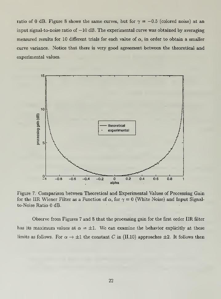
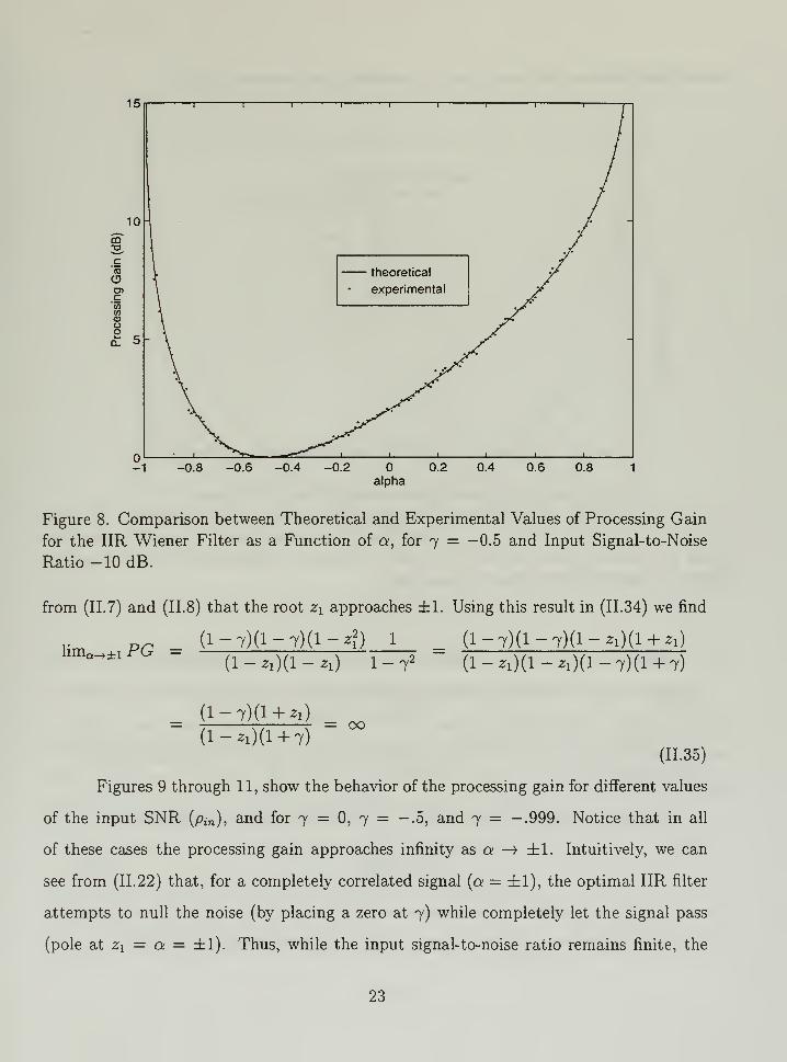
ratio of dB. Figure 8 shows the same curves, but for 7 = —0.5 (colored noise) at an
input signal-to-noise ratio of —10 dB. The experimental curve was obtained by averaging
measured results for 10 different trials for each value of a, in order to obtain a smaller
curve variance. Notice that there is very good agreement between the theoretical and
experimental values.
15
theoretical
experimental
1 i_
-1 -0.8 -0.6 -0.4 -0.2 0.2 0.4 0.6 0.8 1
alpha
Figure 7. Comparison between Theoretical and Experimental Values of Processing Gain
for the IIR Wiener Filter as a Function of a, for 7 = (White Noise) and Input Signal-
to-Noise Ratio dB.
Observe from Figures 7 and 8 that the processing gain for the first order IIR filter
has its maximum values at a = ±1. We can examine the behavior explicitly at these
limits as follows. For a —> ±1 the constant C in (11.10) approaches ±2. It follows then
22
15
Figure 8. Comparison between Theoretical and Experimental Values of Processing Gain
for the IIR Wiener Filter as a Function of a, for 7 = -0.5 and Input Signal-to-Noise
Ratio -10 dB.
from (II.7) and (II. 8) that the root z\ approaches ±1. Using this result in (11.34) we find
(1 - 7)(1 - 7)(1 - z{) 1 (1 - 7)(1 - 7)(1 - *i)(l + *i)limQ-+±l PG =
(1-20(1-2:!) I-72 (l-z1)(l-z1)(l- 7)(l + 7)
(1- 7)(1 + Zl )
(1-20(1 + 7)
= 00
(11.35)
Figures 9 through 11, show the behavior of the processing gain for different values
of the input SNR (p,n ), and for 7 = 0, 7 = —.5, and 7 = —.999. Notice that in all
of these cases the processing gain approaches infinity as a —> ±1. Intuitively, we can
see from (11.22) that, for a completely correlated signal (a — ±1), the optimal IIR filter
attempts to null the noise (by placing a zero at 7) while completely let the signal pass
(pole at z\ — a = ±1). Thus, while the input signal-to-noise ratio remains finite, the
23
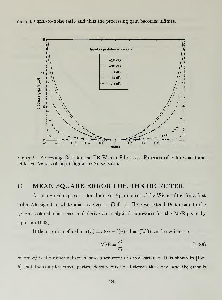
output signal-to-noise ratio and thus the processing gain becomes infinite.
Figure 9. Processing Gain for the IIR Wiener Filter as a Function of a for 7 = and
Different Values of Input Signal-to-Noise Ratio.
C. MEAN SQUARE ERROR FOR THE IIR FILTER
An analytical expression for the mean-square error of the Wiener filter for a first
order AR signal in white noise is given in [Ref. 5]. Here we extend that result to the
general colored noise case and derive an analytical expression for the MSE given by
equation (1.33).
If the error is defined as e(n) = s(n) — s(n), then (1.33) can be written as
~2
MSE =oi
(11.36)
where a\ is the unnormalized mean-square error or error variance. It is shown in [Ref.
5] that the complex cross spectral density function between the signal and the error is
24
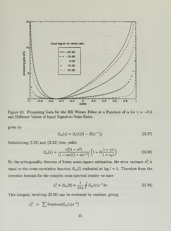
Figure 10. Processing Gain for the IIR Wiener Filter as a Function of a for 7 = —0.5
and Different Values of Input Signal-to-Noise Ratio.
given by
Sa€ (z)=S.(z)(l-H(z-1
)) (11.37)
Substituting (1.22) and (11.22) then yields
saz) = ,G
*{l
:a2) Ji-g 1
(1 - az)(l - az- 1) r ~ 1 - z x z)
(IL38)
By the orthogonality theorem of linear mean-square estimation, the error variance a\ is
equal to the cross-correlation function Rse (l) evaluated at lag / = 0. Therefore from the
inversion formula for the complex cross spectral density we have
o\ = Rse {0) = ^-j SS€ {z)z-l dz
This integral, involving (11.38) can be evaluated by residues, giving
o\ = ^Residues[5se (2;)2_1
]
(11.39)
25
-1 -0.8 -0.6 -0.4 -0.2
Figure 11. Processing Gain for the IIR Wiener Filter as a Function of a for 7 = —.999
and Different Values of Input Signal-to-Noise Ratio.
*2(i - *2)
(1 - az)(l - az' 1
)
l-G 1 — jz
1 — Z\Z
-1 (z-a)
a; il„l~7a\1 — 2ia>
Finally, using this result in (11.36) we obtain
MSE = 1 - G (1 ~ 7g)
(1 - zia )
(11.40)
Figure 12 compares the theoretical mean-square error for 7 = and pin = dB
with the averaged measured squared errors for the same case. Again, there is a good
agreement between the theoretical and the experimental results. Figure 13 shows the
behavior of the mean-square error for input signal-to-noise ratio of —10 dB, dB, and
10 dB. Notice that, when a = 7 = 0, MSE = tf/(a^ + o*). For example, when pin =
26
0.6
0.5
-\ 1 1 1 1 1 1 r
<•- s.-.—
experimentaltheoretical
-1 -0.8 -0.6 -0.4 -0.2 0.2
alpha0.4 0.6 0.8
Figure 12. Comparison between Theoretical and Experimental Values of Mean Square
Error for the IIR Wiener Filter as a Function of a for 7 = (White Noise) and Input
Signal-to-Noise Ratio of dB.
dB, the power of the signal equals the power of the noise, and MSE = 0.5, as expected.
The same analysis for pin = 10 dB results in MSE = 0.1/1.1 w 0.1.
Figure 14 shows a case when the noise is not white (7 = —0.5). The results are
qualitatively similar to those for the white noise case. However the curves are skewed,
indicating that the worse performance in terms of mean-square error occurs when the
signal has a correlation coefficient equal to that of the noise.
D. SIGNAL DISTORTION FOR THE IIR FILTERIn this section we derive an explicit expression for the signal distortion (1.34)
produced by the Wiener filter for the problem of a signal in additive noise. As in the
previous sections, the signal and the noise are each represented by a first order AR model.
27
0.9-
0.8-
2 0.7CD
CD
3 u.u
w
§0.5E
| 0.4
CO
E
| 0.3
0.2
0.1
1 1 1 1 1 1 1 1 1
jr Input signal-to-noise ratio ^k
7 -10 dB
-- OdB
10dB
\ -
/
/
/ - " "
"
- ~~~"^-i
1 -*
"" ** ^ -» l
iy **
* • x/ X
/ \/ \
/ \
/ \
/ \
./ \.
/ \
1 1
L J
i i i i i i i i i
-1 -0.8 -0.6 -0.4 -0.2 0.2
alpha
0.4 0.6 0.8
Figure 13. Mean Square Error for the IIR Wiener Filter as a Function of a for 7(White Noise) and Different Values of Input Signal-to-Noise Ratio.
=
To evaluate the term Rsys {0) in (1.34), we begin with the cross complex spectral
density function between the input and output of the filter is given [Ref. 5] by
Ssys (z) = H(z- l)Ss (z)
Therefore, as before, we can evaluate Rsys (0) from
Rsys {fy = X^ResiduesfS^z),?-1
]
Er. . , „ f l ~lz \ <7?(1 - a2 )z~ l
Residues G —,, ,„
'
rr\\-ziz) {1 - az){l - az~ l
)
The only residue is given by
Residue - G £—^la2 (1 - a2)
(l-ziz)s {l-az)(l-az- l )z- 1 (z-a)
/T2^(1 --7«)= (7 C G-
(1 - zi<x)
(11.41)
(11.42)
28
0.9
0.8
£0.7oCD
§0.6a-in
§0.5E
| 0.4
co
E§0.3
0.2
0.1
7 I 1 ' —I I 1 1 1 I
\r Input signal-to-noise ratio ^V.
-10 dB \.
1 OdB
—10dB
- — — \
^/ ~" — .. \
/"~ — ^ \
/
/ ^^
/ >* i
-/ \ Lv 1
;N 1
i \ 1
i \
i
\
i
\
\
i i i i i i i i i '
-1 -0.8 -0.6 -0.4 -0.2
alpha
0.2 0.4 0.6 0.8
Figure 14. Mean Square Error for the IIR Wiener Filter as a Function of a for 7 =(Colored Noise) and Different Values of Input Signal-to-Noise Ratio.
-0.5
resulting in
jin (1 ~ 7g)Rsys (0) = g]G- (11.43)
Then, by substituting (11.43), (11.30), and Rs (0) = a2s
into (1.34) we can obtain an
expression for signal distortion,
SD = l-j (11-44)
where
E =
F =
(1 ~ 7Qp
(1 - ZiO)
(1 - 7M)(1 - 7*i)(l " o?) (1 - 7/«)(l - ja)+
(11.45)
(11.46)(1 - a?)(l - o*i)(l - a/*) (1 - zi/o)(l - 21a).
Figure 15 shows the theoretical expression (11.44) against the measured results as
a function of the correlation factor cu, for white noise, with an input signal-to-noise ratio
29
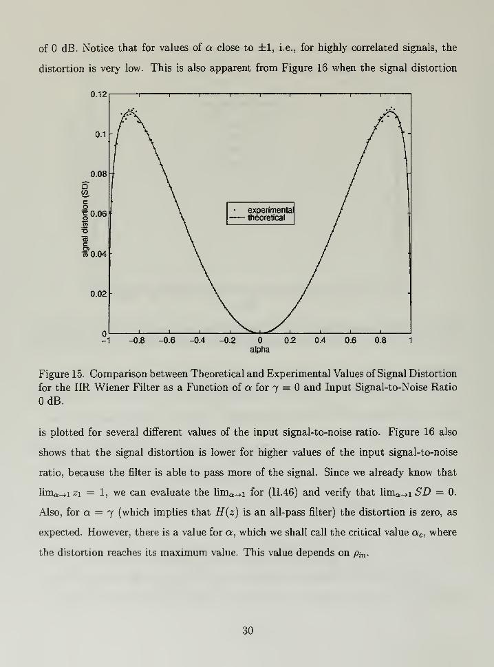
of dB. Notice that for values of a close to ±1, i.e., for highly correlated signals, the
distortion is very low. This is also apparent from Figure 16 when the signal distortion
0.12
0.1 -
0.08
QWc
I0.06
£2
ffi
CO)55 0.04
I I I 1 1 1 i i i
\• experimental
theoretical
/
\ /
1 1 1 j—^-fc.,1^^—1_ i i i
0.02
-1 -0.8 -0.6 -0.4 -0.2 0.2 0.4 0.6 0.8 1
alpha
Figure 15. Comparison between Theoretical and Experimental Values of Signal Distortion
for the IIR Wiener Filter as a Function of a for 7 = and Input Signal-to-Noise Ratio
OdB.
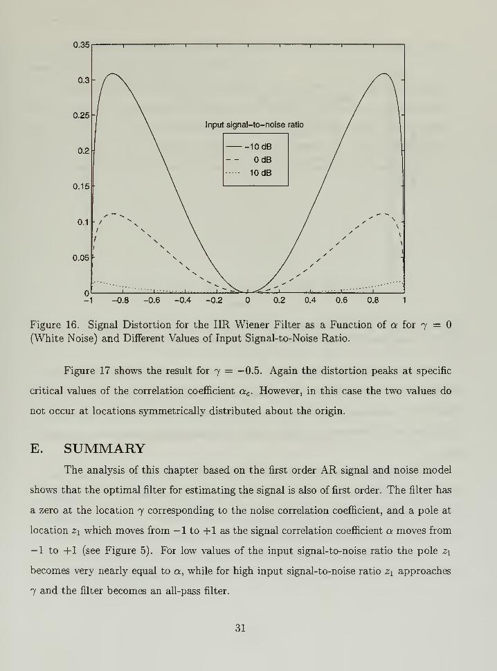
is plotted for several different values of the input signal-to-noise ratio. Figure 16 also
shows that the signal distortion is lower for higher values of the input signal-to-noise
ratio, because the filter is able to pass more of the signal. Since we already know that
lima-n Z\ = 1, we can evaluate the limQ_>i for (11.46) and verify that lima_>.i SD = 0.
Also, for a = 7 (which implies that H{z) is an all-pass filter) the distortion is zero, as
expected. However, there is a value for a, which we shall call the critical value ac , where
the distortion reaches its maximum value. This value depends on pin .
30
0.35
0.3-
0.25-
0.2
0.15 -
0.1
0.05
I I I 1 I 1 I I I
I \ Input signal-to-noise ratio / 1
\-10 dB
OdB
10dB
' ~ ** \ / * " "*\
/ \ / ' V
\ /
-1 -0.8 -0.6 -0.4 -0.2 0.2 0.4 0.6 0.8 1
Figure 16. Signal Distortion for the IIR Wiener Filter as a Function of a for 7 =(White Noise) and Different Values of Input Signal-to-Noise Ratio.
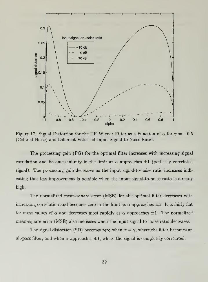
Figure 17 shows the result for 7 = —0.5. Again the distortion peaks at specific
critical values of the correlation coefficient ac . However, in this case the two values do
not occur at locations symmetrically distributed about the origin.
E. SUMMARYThe analysis of this chapter based on the first order AR signal and noise model
shows that the optimal filter for estimating the signal is also of first order. The filter has
a zero at the location 7 corresponding to the noise correlation coefficient, and a pole at
location Z\ which moves from — 1 to +1 as the signal correlation coefficient a moves from
— 1 to +1 (see Figure 5). For low values of the input signal-to-noise ratio the pole z\
becomes very nearly equal to a, while for high input signal-to-noise ratio z\ approaches
7 and the filter becomes an all-pass filter.
31
0.4 0.6 0.8 1
Figure 17. Signal Distortion for the IIR Wiener Filter as a Function of a for 7(Colored Noise) and Different Values of Input Signal-to-Noise Ratio.
= -0.5
The processing gain (PG) for the optimal filter increases with increasing signal
correlation and becomes infinity in the limit as a approaches ±1 (perfectly correlated
signal). The processing gain decreases as the input signal-to-noise ratio increases indi-
cating that less improvement is possible when the input signal-to-noise ratio is already
high.
The normalized mean-square error (MSE) for the optimal filter decreases with
increasing correlation and becomes zero in the limit as a approaches ±1. It is fairly flat
for most values of a and decreases most rapidly as a approaches ±1. The normalized
mean-square error (MSE) also increases when the input signal-to-noise ratio decreases.
The signal distortion (SD) becomes zero when a = 7, where the filter becomes an
all-pass filter, and when a approaches ±1, where the signal is completely correlated.
32
It achieves its maximum values for moderately high values of correlation. In the
case of white noise this occurs around 0.8 < |ac |< 0.9. (see Figure 16).
The performance of the filter for colored noise parallels that of the filter for white
noise. However, the symmetry with respect to a = is lost. When a = 7, the processing
gain goes to zero, the mean-square error achieves its maximum value, and the signal
distortion goes to zero. Maximum values of the signal distortion occur at two distinct
points above and below the value of the noise correlation parameter 7 (see Figure 17).
33
34
III. ANALYSIS OF THE FIR WIENER FILTER
In this chapter we develop expressions for the FIR form of the Wiener filter for
the case where the signal and the noise are, again, each represented by a first order AR
model (equations (1.19) and (1.24)). The chapter is divided into two parts. In Part A, we
derive analytical expressions for the first order FIR Wiener filter, i.e., a FIR filter with
only two coefficients. In Part B, we use a more general approach to derive expressions
for a filter of any order. Although Part A treats a restricted particular case, it allows us
to obtain simple expressions for the measures of performance as functions of the model
parameters. On the other hand, the results of Part B permit us to plot the measures of
performance for more general cases, where the FIR filter can be of any order.
A. THE FIRST ORDER FIR WIENER FILTER
In Chapter I we introduced the matrix form of the Wiener-Hopf equation (1.16)
for the FIR Wiener filter and the associated mean-square error (1.17). For the first
order FIR Wiener filter, the vector of filter coefficients h has only two elements, i.e.,
h = [h(0) h(l)]T
. Thus we can obtain expressions for these two coefficients by solving
equation (1.16) as follows. Since the noise is assumed uncorrelated with the signal, Rx (l)
and Rsx (l) are given by (1.3) and (1.4). Evaluating (1.20) and (1.25) for lag / = and 1,
and substituting in (1.3) yields
Rx (0) = a2 + a2 = a2[l + pin }
(III.l)
and
RX {1) = a2a + a2j = a2
[j + apin ](III.2)
Similarly, from (1.20) and (1.4) we obtain
RsM = v2
s(HI.3)
35
and
Rsx (l) = aas
Using (III.l) through (III.4) in equation (1.16) results in
(III.4)
[MO)
"
«*J1
[ Mi) ja
(pin + 1) (aPin + j)
{apin + 7) (pin + 1)
Then, solving this matrix equation by inverting the matrix, we can express the filter
coefficients as
MO)
Mi) (pin + l) 2 - (apin + 7)'
pin + l -(Olpin + l)
-(aPin+j) Pin + 1
or,
MO) = Pi(pin + 1 - a2
Pin - ui)
(pin + l) 2 - (Upin + 7)2
Ml) == Pir
(a--7)1 1
(Pin + 1)2 -
• (apin + 7)2
The transfer function for the filter is then given by
H(z) = h(0) + h(l)z-1
or
H(z) = h(0)(l-z z- 1
)
where the zero of the filter is located at
z = z = - Mi)
Ho)
or
Zq =(7 -a)
(pin + 1 - a2pin -ay)
1
a
(III.5)
(III.6)
(III.7)
(III.8)
(III.9)
Figures 18 and 19 show the location of the zero z of the first order FIR Wiener
filter as a function of a for different values of 7, and for an input signal-to-noise ratio of
dB and —10 dB, respectively. From these figures we can identify three interesting cases.
36
cc
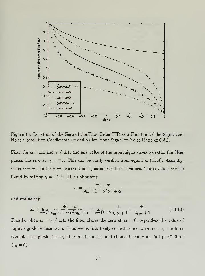
Figure 18. Location of the Zero of the First Order FIR as a Function of the Signal and
Noise Correlation Coefficients (a and 7) for Input Signal-to-Noise Ratio of dB.
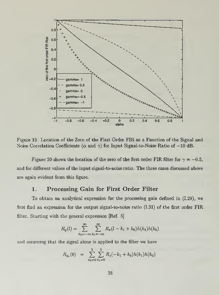
First, for a = ±1 and 7 ^ ±1, and any value of the input signal-to-noise ratio, the filter
places the zero at z = Tl* This can be easily verified from equation (III.9). Secondly,
when a = ±1 and 7 = ±1 we see that z assumes different values. These values can be
found by setting 7 = ±1 in (III. 9) obtaining
±l-az =
pin + 1 - a2pin =F a
and evaluating
z = lim±l-a = lim
1 ±1(111.10)
*"*" Pin + 1 - C^2Pin ¥ Ot a^±\ -2apin =F 1 ^Pin + 1
Finally, when a = 7 ^ ±1, the filter places the zero at zo = 0, regardless the value of
input signal-to-noise ratio. This seems intuitively correct, since when a = 7 the filter
cannot distinguish the signal from the noise, and should become an "all pass" filter
(*o = 0).
37
1
0.8
0.6
0.4
0.2
-0.2
-0.4
-0.6
-0.8
-1
• _ ' I ~T 1 1 1 1 1 1
+ °\ """-^ ' ,^__
- + % **• -« -
+ '%+ \+ *•••. "* «„
+++ \+ X.+++ V N+ X. N+ V \+++
. V+ . %. \
++ \" gamma= 1
— gamma= 0.5
gamma=
_ + gamma=-0.5
++ \
++4. '-. \
gamma= -1
-0.8 -0.6 -0.4 -0.2 0.2 0.4 0.6 0.8 1
alpha
Figure 19. Location of the Zero of the First Order FIR as a Function of the Signal and
Noise Correlation Coefficients (a and 7) for Input Signal-to-Noise Ratio of —10 dB.
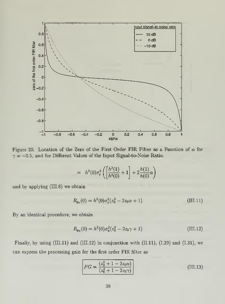
Figure 20 shows the location of the zero of the first order FIR filter for 7 = —0.5,
and for different values of the input signal-to-noise ratio. The three cases discussed above
are again evident from this figure.
1. Processing Gain for First Order Filter
To obtain an analytical expression for the processing gain defined in (1.29), we
first find an expression for the output signal-to-noise ratio (1.31) of the first order FIR
filter. Starting with the general expression [Ref. 5]
00 00
fco=— 00 fci=—00
and assuming that the signal alone is applied to the filter we have
JU°) = EE^K +WWo)fco=0 fci=0
38
1fc
i i i i— i T I I 1
nput siqnal-to noise ratio
0.8 10 dB-
1v '
- - OdB| 0.6
1
v• -10 dB
-
**~1
N
oc1
N '
t 0.4 _\ \ '•. -
0) \ N '•
T3 \ \ .wO \ s
2 °-2 " \ v•
-
\ s. '•
•is \. N.
<D ^^~-^^. V '.
r ° ".>. '
-
"o •.""" ^o '-.. "* »»
g-0.2"-^ >v
-0.4
'
' • *** \
-0.6' ' " • ***' \'"• N
\
-0.8
1 1 1 1 1
"* N V
"'•' V\
1 1 1 1
-1 -0.8 -0.6 -0.4 -0.2 0.2 0.4 0.6 0.8 1
alpha
Figure 20. Location of the Zero of the First Order FIR Filter as a Function of a for
7 = —0.5, and for Different Values of the Input Signal-to-Noise Ratio.
= h2(Q)a
h2(l)
h2(0)
+ 1 8Kand by applying (III. 8) we obtain
Rys (0) = h2
(0)ai(z2 -2z a + l) (111.11)
By an identical procedure, we obtain
Ryr,(0) = h2(0)a*(z
2 - 2207 + l) (111.12)
Finally, by using (III.ll) and (111.12) in conjunction with (11.11), (1.29) and (1.31), we
can express the processing gain for the first order FIR filter as
PG(z% + 1 - 2zQa)
{zl + l- 2z 7)(111.13)
39
3.5
theoretical
experimental
_i [_ _i i_
-1 -0.8 -0.6 -0.4 -0.2 0.2 0.4 0.6 0.8 1
alpha
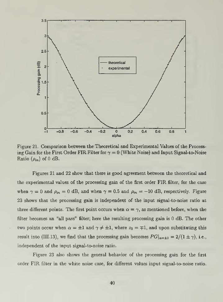
Figure 21. Comparison between the Theoretical and Experimental Values of the Process-
ing Gain for the First Order FIR Filter for 7 = (White Noise) and Input Signal-to-Noise
Ratio (pin ) of dB.
Figures 21 and 22 show that there is good agreement between the theoretical and
the experimental values of the processing gain of the first order FIR filter, for the case
when 7 = and pin = dB, and when 7 = 0.5 and pin = —10 dB, respectively. Figure
23 shows that the processing gain is independent of the input signal-to-noise ratio at
three different points. The first point occurs when a = 7, as mentioned before, when the
filter becomes an "all pass" filter; here the resulting processing gain is dB. The other
two points occur when a = ±1 and 7 ^ ±1, where z = =pl, and upon substituting this
result into (III. 13), we find that the processing gain becomes PG|a=± i= 2/(1 ±7), i.e.,
independent of the input signal-to-noise ratio.
Figure 23 also shows the general behavior of the processing gain for the first
order FIR filter in the white noise case, for different values input signal-to-noise ratio.
40
o-
-1
theoretical
experimental
j i i i i i_
-1 -0.8 -0.6 -0.4 -0.2 0.2 0.4 0.6 0.8 1
alpha
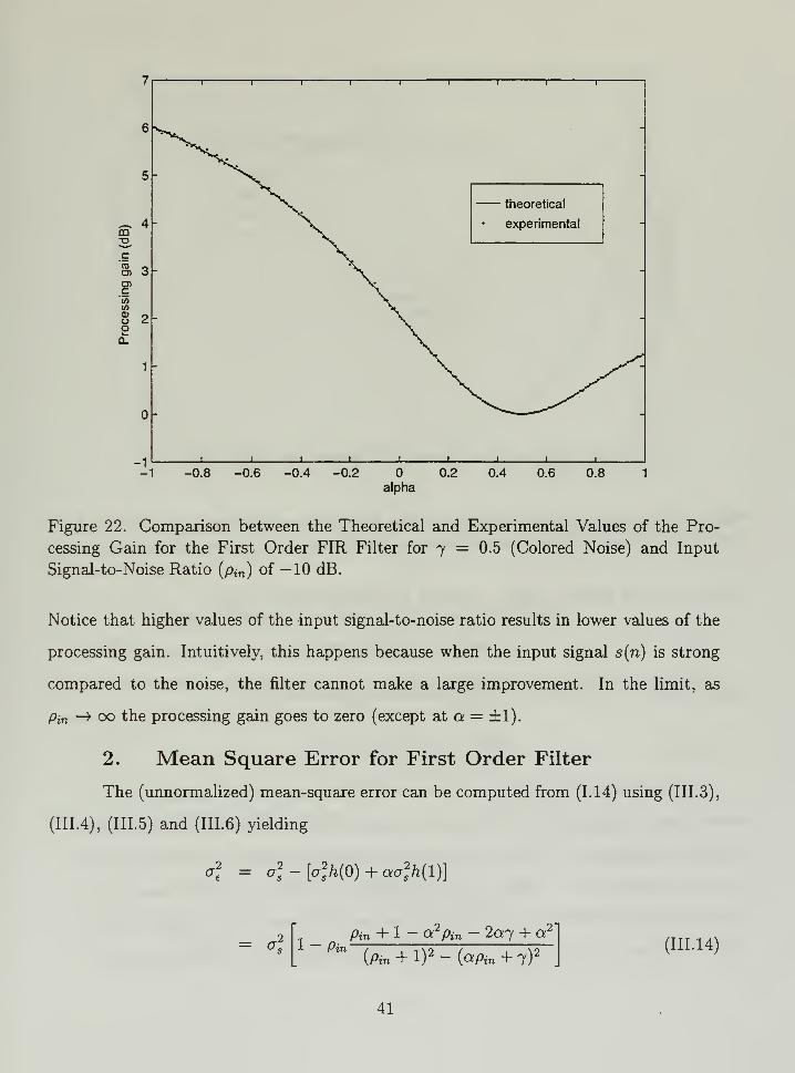
Figure 22. Comparison between the Theoretical and Experimental Values of the Pro-
cessing Gain for the First Order FIR Filter for 7 == 0.5 (Colored Noise) and Input
Signal-to-Noise Ratio (p,n) of —10 dB.
Notice that higher values of the input signal-to-noise ratio results in lower values of the
processing gain. Intuitively, this happens because when the input signal s(n) is strong
compared to the noise, the filter cannot make a large improvement. In the limit, as
Pin -» 00 the processing gain goes to zero (except at a = ±1).
2. Mean Square Error for First Order Filter
The (unnormalized) mean-square error can be computed from (1.14) using (III. 3),
(III.4), (III.5) and (III.6) yielding
a\ = a2s-[a2
sh(0)+aa2
sh(l)}
= cr c 1 -PiPin + 1 a2
pin 2oi7 4- a2
(Pin + I) 2 - (apin + l)''
(111.14)
41
7 1 1 1 1 1 1 1 1 1
6 r».
n. Input signal-to-noise ratio• v
x>.
-- -10 dB5
OdB~
m x 10 dB2, I N
.£4CO
\ S
\ S"
O) \ 'V
O) \ Vc \ N"w \ N0) o \ Vo \ so \ N0_ \ '•
N
2 \ N
X \\ \
1\. •. y 1-\ •• v '.'' /^^ \ y- /^^^^ '• N y^ /
"—-~~—_ '"'•N <''\^0y^r\ i i i i i
•>. -
i f 'j 1
-1 -0.8 -0.6 -0.4 -0.2 0.2 0.4 0.6 0.8 1
alpha
Figure 23. Processing Gain for the First Order FIR Filter as a Function of a, for 7 =(White Noise) , and Different Input Signal-to-Noise Ratio.
Alternatively, by applying (III. 8), it can be written as a function of z :
0* = o*[l - h(0)[l - a*] (111.15)
Using (III. 15) in (1.33) gives the normalized mean-square error as
MSE = [l-/i(0) [1-azo] (111.16)
Figures 24 and 25 compare the theoretical and experimental values of the nor-
malized mean-square error for different values of input signal-to-noise ratio and the noise
correlation parameter 7. Again, there is a good agreement between the theoretical and
the experimental curves. Figure 26 shows the behavior of the normalized mean-square
error for different values of input signal-to-noise ratio. We see that for higher values of
the input signal-to-noise ratio the mean-square error assumes lower values, as expected.
42
0.55
0.3
0.25-
0.2
-i1
1 1 1 1 1 r
theoretical
experimental
-1 -0.8 -0.6 -0.4 -0.2 0.2 0.4 0.6 0.8 1
alpha
Figure 24. Comparison between the Theoretical and Experimental Values of the Mean-
Square Error for the First Order FIR Filter for 7 = (White Noise) and Input Signal-
to-Noise Ratio of dB.
3. Signal Distortion for First Order Filter
The signal distortion defined by (1.34) is easily evaluated. It is easy to show that
the cross correlation between input and output of a linear system is related to the input
autocorrelation function by the convolution relation [Ref. 5]
A:=—00
Hence, for our first order filter we have
(111.17)
RsyM = Y, h(k)Rs (-k)
= a2
s(h(0) + ah(l))
= a2
sh{0)(l - azQ ) (111.18)
43
0.1
0.03
0.02-
0.01
theoretical
experimental
j i_ J I I L
-1 -0.8 -0.6 -0.4 -0.2 0.2 0.4 0.6 0.8 1
alpha
Figure 25. Comparison between the Theoretical and Experimental Values of Mean-
Square Error for the First Order FIR Filter as Function of a for 7 = 0.5 (Colored Noise)
and Input Signal-to-Noise Ratio of —10 dB.
Then, by applying (111.18) and (III.ll) to (1.34), we obtain
SD = *o2(l ~ <*
2)
1 — 2az + z\(111.19)
Figure 27 shows the theoretical and experimental values of the signal distortion
for different values of a, and for 7 = (white noise) at a input signal-to-noise ratio of
dB. We again observe good agreement between the experimental and theoretical results.
As in the case of the IIR filter, the distortion is zero for a = 7 and a = dbl, and achieves
a maximum value at a point < ae < 1. In Figures 28 and 29, the noise parameter
7 has fixed values of (white noise) and 0.5, respectively, and the signal distortion is
plotted for different values of the input signal-to-noise ratio. Notice that for lower values
of input signal-to-noise ratio the signal distortion assumes higher values. In addition,
44
1
0.9
0.8
1 i T 1 1I 1 i i
Input signal-to-noise ratio
"^^k_
-- -10 dB2 0.7o
-
OdB-
2 10 dB§0.6(0
c8 0.5 -
Eo.§0.4
'''••.,
E
J0.3- -
0.2 -
0.1
n 1 i i i i i i i i
-1 -0.8 -0.6 -0.4 -0.2 0.2 0.4 0.6 0.8 1
alpha
Figure 26. Mean-Square Error for the First Order FIR Filter as a Function of a for
7 = 0.5 (Colored Noise) for Different Values of Input Signal-to-Noise Ratio.
notice that, regardless of the input signal-to-noise ratio, for a = 7 or for a = ±1, the
signal distortion is zero. This can also be easily verified from (III. 19).
B. PERFORMANCE MEASURES FOR HIGHER ORDERFIR WIENER FILTERS
For FIR filters of higher than first order (P > 2), it becomes extremely difficult
or impossible to derive analytical expressions for the filter coefficients and zeros of the
filter in term of the basic parameters a, 7, and pin . However it is still useful to be
able to compute theoretical values for the processing gain, mean-square error, and signal
distortion in these cases. Therefore, in this section we develop a different approach to
derive expressions for these performance measures, which can be plotted as a function
of the various parameters. With these results, we can compare the performance the FIR
45
0.06
Figure 27. Comparison between the Theoretical and Experimental Values of Signal Dis-
tortion for Different Values of a and for 7 = (White Noise) at a Input Signal-to-Noise
Ratio of dB.
filter of any order to that of the optimal IIR Wiener filter when they are applied to the
first order signal and noise models of equations (1.19) and (1.24).
1. Processing Gain for Higher Order FIR Filter
The output power of a filter expressed in the form (1.15) can be written as
Rs (0) = E{y2(n)}
= E{(hrx)(xrh)}
= hrE{xxr}h
= hrRxh (111.20)
Therefore, the output power when the signal and noise act alone is given by
/^s (0) = hTRsh (111.21)
46
0.12
0.1
-i 1 1 1 1 1 1 r
Input signal-to-noise ratio
/ \/ \
\
\
- - -10 dB
OdB
10 dB
/• \/ \
/
/
\ /
Figure 28. Signal Distortion for the First Order FIR Filter as a Function of a. for 7 =and Different Values of the Input Signal-to-Noise Ratio
and
i^(0) = hTIVi (111.22)
where Rs and R^ are the signal and the noise correlation matrices, which have the form
Rs—
J a2a •• a2sa\p- 1
cr2sa *2
sa2
sa\p~2
.°2s<x
]P-•i| a]*\p-2|
. ' o2
< °\l .. a?7|P-l|
R77 — "li < • a,27|P-21
. ^7|P-"
CT27IP-2| . •• <
(111.23)
Thus from (111.21), (111.22), (1.29) and (1.31) we obtain
rTR^h 1PG
l^R^h pi
(111.24)
47
0.25
0.2
f 0.15|-
gTo
"rac
55 0.1
0.05
1 1 1 r n r
Input signal-to-noise ratio
- - -10 dB
OdB
10 dB
/
/
/ .
/.-'
/
.
/.
Figure 29. Signal Distortion for the First Order FIR Filter as Function of a for 7 = 0.5
and Different Values of the Input Signal-to-Noise Ratio
The processing gain produced by the Wiener filter can be obtained by substituting the
solution to the Wiener-Hopf equation (1.16) into (III. 24). Specifically, from (1.16) and
(1.18) we have
h = (Rs -r-R7?)- 1
f5 (111.25)
Since we have all the necessary expressions, we can plot the values assumed by the
processing gain (III.24) for different values of a, 7, and pin .
Figure 30 shows the behavior of the processing gain as a function of a for 7 =
(white noise) and for different values of input signal-to-noise ratio. Notice that the
processing gain has different maxima for a = ±1, depending on the order of the filter.
These maximum values can be easily predicted for the white noise case (7 = 0), as
48
follows. For a = 1 and 7 = the signal and noise correlation matrices (III. 23) become
Rs —
2 2
R-T7 —
Under these conditions (III.25) shows that h(0)
these results to (III.21) and (III. 22), we obtain
<
h(l) = .
(111.26)
= h(P - 1). By applying
hTR4h = P2aJfc
2(0)
and
hrRr?h = a2 P/i2
(0)
Finally, substituting these expressions into (III. 24) results in
PG = P
A similar analysis shows that PG = P also for a = — 1.
This result shows that unlike the IIR filter, the processing gain for an FIR has
a finite bound, which is equal to the filter length. This result can be easily checked in
Figure 30.x Notice also that in general, for any value of a, larger length filters produce
increased processing gain.
2. Mean Square Error for Higher Order FIR Filter
The normalized mean-square error (1.33) for any FIR filter is not difficult to obtain.
Using (1.15) and (1.1) we can write
E{{s{n)-y(n)) 2} = E {(s{n) - hT s - hT T))(s(n) - s
T h - rf h)}
= a] - 2 hT fs + hT Rs h + hr R,, h
1 Note that the vertical scale in Figure 30 is in dB
49
9
i i I I 1 i i i r
8
filter length
\-
7
S" 6
2
42,c(0 10o>
g> 5 i -
<ft
(ft
m8£ 4
3
•>. \ ,
if
2
1
r\ I I 1 1I _c "I 1 1 1
-0.8 -0.6 -0.4 -0.2
alpha
0.2 0.4 0.6 0.8
Figure 30. Processing Gain for the FIR Filter of Length P for 7 = (White Noise) and
Input Signal-to-Noise Ratio of dB
where the cross terms disapear because the signal and noise are uncorrelated. Then,
substituting this expression in (1.33) we obtain
2hr fs -hT Rs h-hT R1,hMSE = 1 - (111.27)
The result (III.27) applies to any FIR filter. For the Wiener filter we can simplify
the expression by noting from (1.16) and (1.18) that
(Rs 4- R77)h - fs =
Therefore, for the Wiener filter (III.27) simplifies to
hr f sMSE = 1
This result can also be obtained directly using (1.17).
(111.28)
50
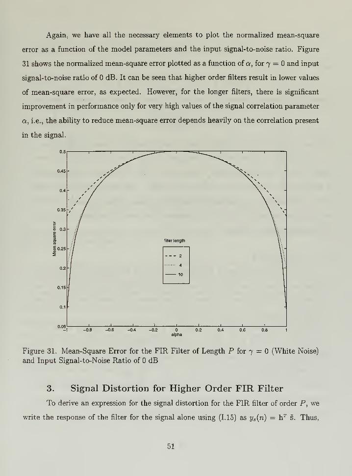
Again, we have all the necessary elements to plot the normalized mean-square
error as a function of the model parameters and the input signal-to-noise ratio. Figure
31 shows the normalized mean-square error plotted as a function of a, for 7 = and input
signal-to-noise ratio of dB. It can be seen that higher order filters result in lower values
of mean-square error, as expected. However, for the longer niters, there is significant
improvement in performance only for very high values of the signal correlation parameter
a, i.e., the ability to reduce mean-square error depends heavily on the correlation present
in the signal.
Figure 31. Mean-Square Error for the FIR Filter of Length P for 7 = (White Noise)
and Input Signal-to-Noise Ratio of dB
3. Signal Distortion for Higher Order FIR Filter
To derive an expression for the signal distortion for the FIR filter of order P, we
write the response of the filter for the signal alone using (1.15) as ys (n) = hT s. Thus,
51
we have
E {s(n)ys (n)} = E {s(n) hT s} = hT fs (111.29)
and
E {ys {n)2} =E{h
Ts s
T h} = hT Rs h (111.30)
Substituting these expressions into equation (1.34) then produces the desired expression
SD = ] -ifefe (IIU1)
This can be evaluated for the Wiener filter by substituting the solution (III.25) for h.
Figure 32 shows the behavior of the signal distortion for the FIR filter of different
orders P, for 7 = and input signal-to-noise ratio of dB. The behavior of this measure
is similar to its behavior in the case of the IIR filter. The signal distortion is dB
for a = ±1 and for a = 7 and achieves a maximum value around a value ae w ±0.8,
depending on the length of the filter. In addition, the value of the signal distortion is
greater for larger filter lengths.
C. SUMMARYThe analysis carried out in this chapter for the FIR Wiener filter shows that this
filter has performance qualitatively similar to that of the IIR filter, although for the case
of a first order AR signal and noise model the performance, in terms of the mean-square
error and processing gain, is never quite as good.
For the first order FIR filter, which has a single zero, the location of the zero
changes from +1 to —1 as the signal correlation coefficient increases from —1 to +1.
When the signal and noise have the same correlation coefficient (a = 7) the zero moves
to the origin (resultind in an all-pass filter); when both signal and noise are perfectly
correlated (a = 7 = ±1) the zero moves to a location that depends on the input signal-
to-noise ratio (see (III. 10)). This results in a steady state estimate for the signal which
is equal to a constant fraction of the input observation sequence.
52
0.12
0.1
0.08-
coco
=5 0.06 1-
~mc
CO
0.04
0.02
I I I I r i i —
i
1
-
filter lengt 1 / -
- - 2
"* ~ ** \' v \
/ \ \I: / \ \
' N \.
.
:
/ A
: ' \:
' \
\/ \
4
10/ ^ ~~
•>.
/ ' x
/''' ^// ^ '
// \
// \
/' »
/ X
/
-
\
i i t i^^
i .^-' 1 1 l l
\
-1 -0.8 -0.6 -0.4 -0.2 0.2 0.4 0.6 0.8 1
alpha
Figure 32. Signal Distortion for the FIR Filter of Length P for 7 = (White Noise) and
Input Signal-to-Noise Ratio of dB
The performance measures for the FIR filter approaches those of the IIR filter as
the order of the filter increases. Figures 30, 31, and 32 show plots of the three performance
measures for the FIR Wiener filter of orders 2, 4, and 10. These performances can be
compared to those for the IIR Wiener filter in Figures 33, 34, and 35. A significant
difference between the two types of filters is that the processing gain of the FIR filter,
when the input signal is perfectly correlated is not infinite, but is limited to a value P
(the filter length). Also the mean-square error does not go to zero when a = ±1 as in
the IIR filter case. However, the signal distortion for the FIR filter does go to zero for
a = 7 and a = ±1, as in the IIR filter, and it is not as large as for the IIR filter.
53
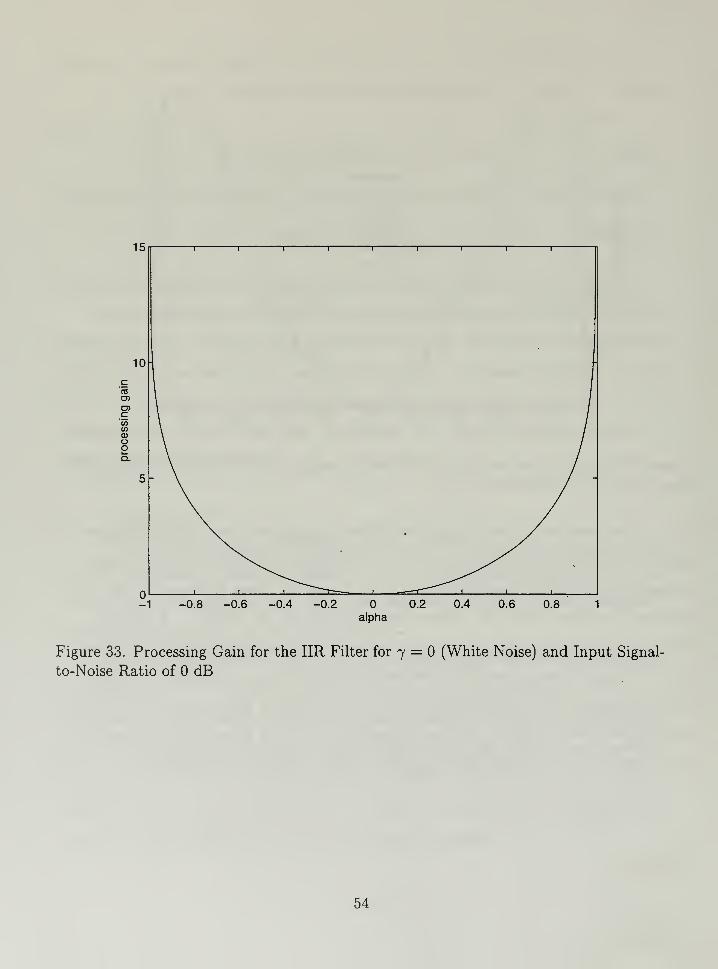
15 1 r t 1
i r 1 r
-1 -0.8 -0.6 -0.4 -0.2 0.2 0.4 0.6 0.8 1
alpha
Figure 33. Processing Gain for the IIR Filter for 7 = (White Noise) and Input Signal-
to-Noise Ratio of dB
54
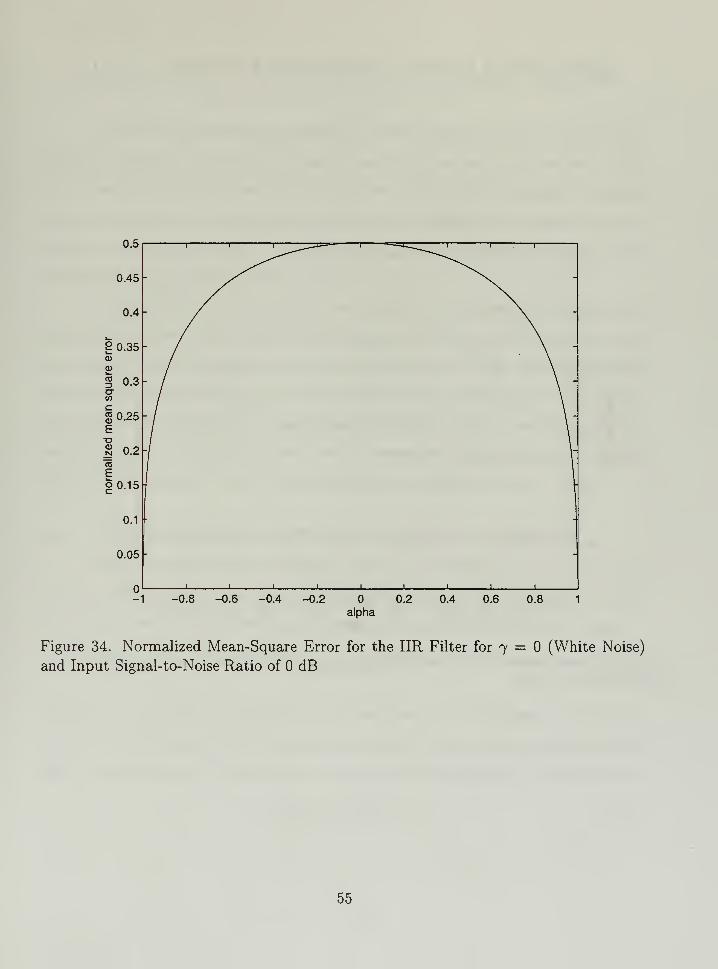
Figure 34. Normalized Mean-Square Error for the IIR Filter for 7 = (White Noise)
and Input Signal-to-Noise Ratio of dB
55
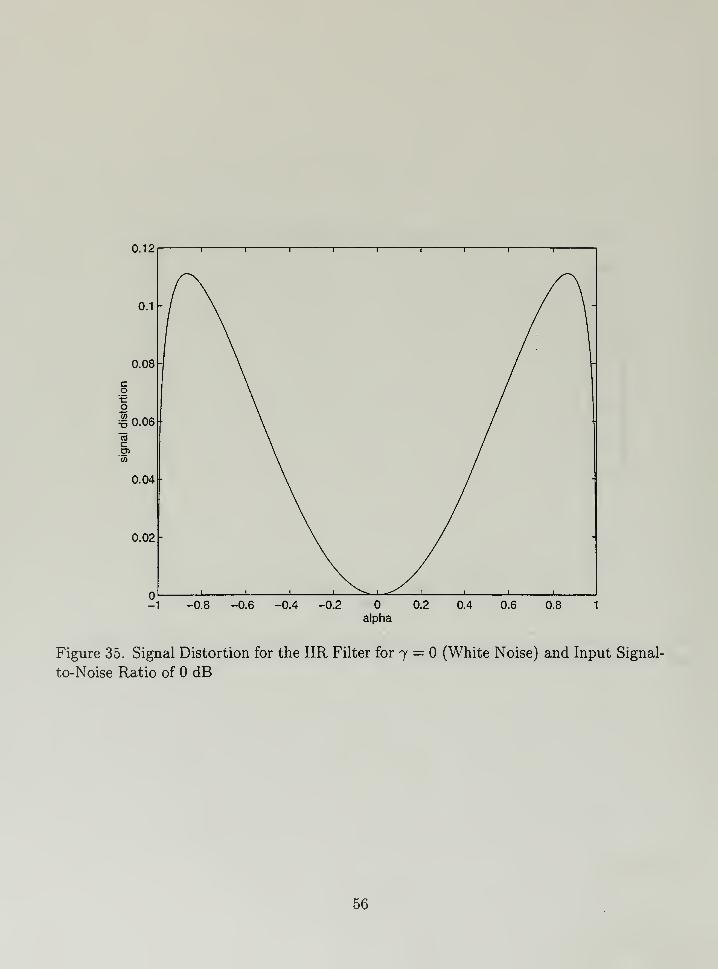
0.12
1
1 1 1 1 1 1 1 1 r
Figure 35. Signal Distortion for the IIR Filter for 7 = (White Noise) and Input Signal-
to-Noise Ratio of dB
56
IV. THE EXTENDED OPTIMAL FILTER
We can conclude from the results of the previous chapters that the Wiener filter,
although optimal in the mean-square error sense, is not necessarily optimal with regard
to minimizing the signal distortion. This chapter addresses the possibility to improve
the signal distortion performance of the filter, at the expense of increasing the output
residual noise. In other words, we may be able to improve the signal intelligibility with
some slight increase in mean-square error due to noise.
Ephraim and Van Trees [Ref. 7] have suggested a more general filter for speech
enhancement, based on one measure of the signal distortion; here we have adapted this
idea using the signal distortion measure defined in Chapter I. This chapter formulates
this more general problem and derives the solution using an FIR filter. It then provides
an analysis of the performance of the generalized FIR filter for the first order AR signal
and noise model, and finally suggests how the generalized filter may be used to obtain
an appropriate trade-off between signal distortion and mean-square error.
A. THE EXTENDED OPTIMAL FILTER PROBLEMWe begin with the filter depicted in Figure 3, and the responses ys (n) and yv {n)
due to the filter acting on the signal and noise alone. The problem as suggested in [Ref.
7] is to minimize the distortion while constraining the residual noise power to satisfy
E {y*(n)} < ol
'
(IV.l)
where of is some chosen level of residual noise power. In this chapter, we apply this
procedure using the signal distortion measure defined in (1.34). In the context of an FIR
filter, the problem can be formulated as to minimize (III.31) subject to the constraint
E{y2
v(n)} = hTRT7
h<crr2
(IV.2)
57
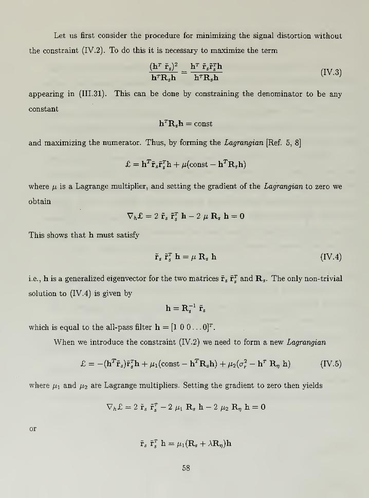
Let us first consider the procedure for minimizing the signal distortion without
the constraint (IV. 2). To do this it is necessary to maximize the term
flg^£ =hT *'*?h
fly 3)hTR5h hTRsh
v }
appearing in (III. 31). This can be done by constraining the denominator to be any
constant
hTRsh = const
and maximizing the numerator. Thus, by forming the Lagrangian [Ref. 5, 8]
£ = hTfsfJh + //(const - hTR5h)
where \i is a Lagrange multiplier, and setting the gradient of the Lagrangian to zero we
obtain
Vft£ = 2fs fJh-2/iRs h =
This shows that h must satisfy
f, fI h = fjL Rs h (IV.4)
i.e., h is a generalized eigenvector for the two matrices fs rj and Rs . The only non-trivial
solution to (IV.4) is given by
h = r; 1fs
which is equal to the all-pass filter h = [1 . . . 0]T
.
When we introduce the constraint (IV. 2) we need to form a new Lagrangian
£ = -(hTfs )fTsh + & (const - hTRsh) + ft{crj - hT R,, h) (IV.5)
where ft and ft are Lagrange multipliers. Setting the gradient to zero then yields
X7 h£ = 2 fs fTs- 2 ft Rs h - 2 ft R^ h =
or
f s fj h = // 1 (Rs + ART/)h
58
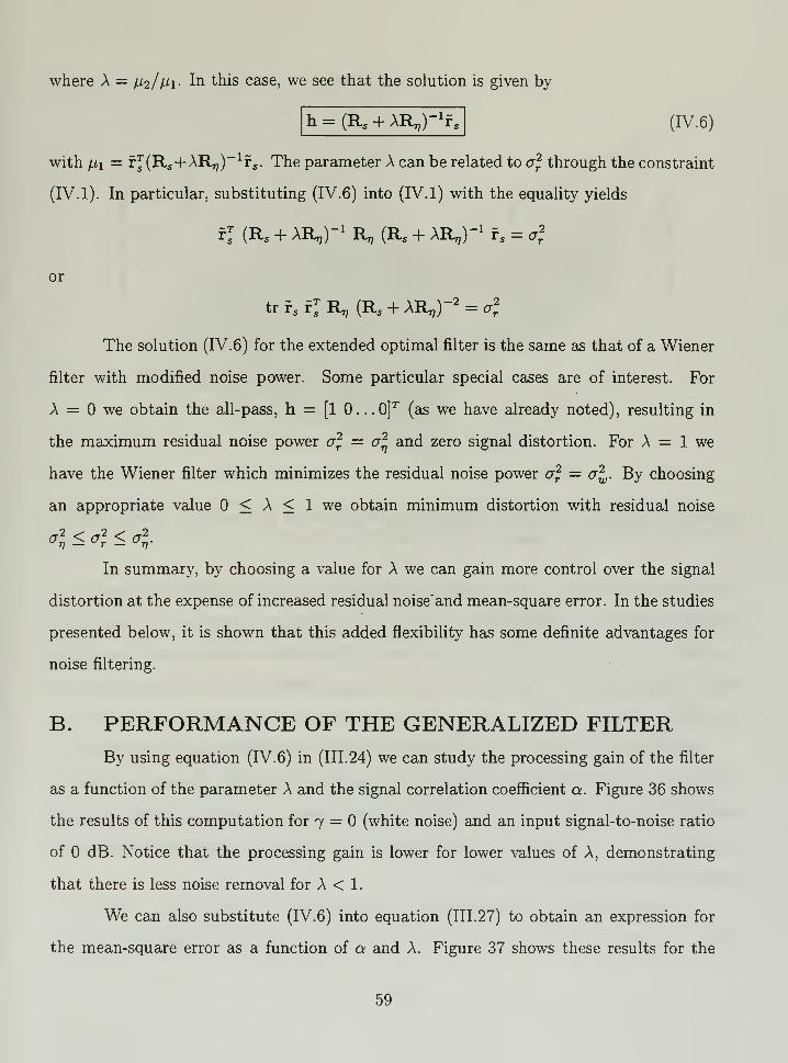
where A = 112/^1- I*1 this case, we see that the solution is given by
h = (R5 + AR7?
)" 1fs (IV.6)
with /i! = fJ(RS+AR^)1 fs . The parameter A can be related to o2 through the constraint
(IV. 1). In particular, substituting (IV.6) into (IV. 1) with the equality yields
fTs(R, + AR,)" 1 R^ (Rs + AR,,)"
1f5 = a2
r
or
trf.fjR,, (Rs + AR„)-2 = ar
2
The solution (IV.6) for the extended optimal filter is the same as that of a Wiener
filter with modified noise power. Some particular special cases are of interest. For
A = we obtain the all-pass, h = [1 0...0]T
(as we have already noted), resulting in
the maximum residual noise power a2 = a2 and zero signal distortion. For A = 1 we
have the Wiener filter which minimizes the residual noise power cr2 = a2
. By choosing
an appropriate value < A < 1 we obtain minimum distortion with residual noise
A < °l < 4In summary, by choosing a value for A we can gain more control over the signal
distortion at the expense of increased residual noise'and mean-square error. In the studies
presented below, it is shown that this added flexibility has some definite advantages for
noise filtering.
B. PERFORMANCE OF THE GENERALIZED FILTER
By using equation (IV.6) in (III.24) we can study the processing gain of the filter
as a function of the parameter A and the signal correlation coefficient a. Figure 36 shows
the results of this computation for 7 = (white noise) and an input signal-to-noise ratio
of dB. Notice that the processing gain is lower for lower values of A, demonstrating
that there is less noise removal for A < 1.
We can also substitute (IV.6) into equation (III.27) to obtain an expression for
the mean-square error as a function of a and A. Figure 37 shows these results for the
59
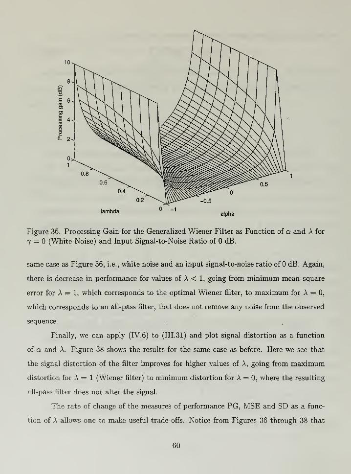
lambda -1alpha
Figure 36. Processing Gain for the Generalized Wiener Filter as Function of a and A for
7 = (White Noise) and Input Signal-to-Noise Ratio of dB.
same case as Figure 36, i.e., white noise and an input signal-to-noise ratio of dB. Again,
there is decrease in performance for values of A < 1, going from minimum mean-square
error for A = 1, which corresponds to the optimal Wiener filter, to maximum for A = 0,
which corresponds to an all-pass filter, that does not remove any noise from the observed
sequence.
Finally, we can apply (IV.6) to (III.31) and plot signal distortion as a function
of a and A. Figure 38 shows the results for the same case as before. Here we see that
the signal distortion of the filter improves for higher values of A, going from maximum
distortion for A = 1 (Wiener filter) to minimum distortion for A = 0, where the resulting
all-pass filter does not alter the signal.
The rate of change of the measures of performance PG, MSE and SD as a func-
tion of A allows one to make useful trade-offs. Notice from Figures 36 through 38 that
60
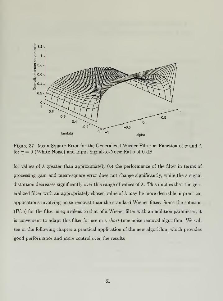
lambda -1alpha
Figure 37. Mean-Square Error for the Generalized Wiener Filter as Function of a and A
for 7 = (White Noise) and Input Signal-to-Noise Ratio of dB
for values of A greater than approximately 0.4 the performance of the filter in terms of
processing gain and mean-square error does not change significantly, while the s signal
distortion decreases significantly over this range of values of A. This implies that the gen-
eralized filter with an appropriately chosen value of A may be more desirable in practical
applications involving noise removal than the standard Wiener filter. Since the solution
(IV. 6) for the filter is equivalent to that of a Wiener filter with an addition parameter, it
is convenient to adapt this filter for use in a short-time noise removal algorithm. We will
see in the following chapter a practical application of the new algorithm, which provides
good performance and more control over the results
61
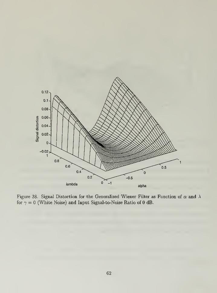
lambda -1alpha
Figure 38. Signal Distortion for the Generalized Wiener Filter as Function of a and A
for 7 = (White Noise) and Input Signal-to-Noise Ratio of dB.
62
V. APPLYING EXTENDED OPTIMALFILTERING TO UNDERWATER SIGNALS
A. INTRODUCTIONIn this chapter we apply the solution of the extended optimal filter expressed
in (IV. 6) to the short-time filtering algorithm developed by Frack in [Ref. 4]. This
algorithm assumes that both the signal and the noise correlation functions (Rs (l) and
Rr,(l)) are unknown a priori; therefore they must be estimated from the data at hand.
Since only x(n) = s(n)+r)(n) is observed, however, only Rx(l) can be estimated directly.
Nevertheless the nature of the problem provides a way to compute the needed statistics.
Since the signal is very short (on the order of seconds or milliseconds) compared to the
time over which the noise statistics are likely to change, an estimate for i^(/) can be
made from the received data prior to the onset of s(n). By using (1.3), this estimate can
in theory be subtracted from Rx (l) to produce an estimate of Rs (l).
Although there is no explicit analytic expression for the parameter A, we can
obtain the value of A corresponding to any desired residual noise level by solving (A). In
the case of white noise, this is equivalent to writing (IV. 2) as
a$hTh = a\||h
||
2= ol (V.l)
and then ( by IV. 6) solving for A from
||(Rs + AH,)" 1
*,||
2=2f (V.2)
Therefore, by setting the level of the residual noise o"l that can be tolerated, we can
assign values for A in each segment by iterating on (V.2) until the equality is satisfied,
thus obtaining the value of A that minimizes the signal distortion. Thus, in principle, all
of the quantities to perform the extended optimal filtering over a short time interval can
be computed, and this can be repeated over successive blocks of data.
The estimate of Rs (l) by subtraction of the estimated correlation functions is
not well formed because there is no guarantee that such an estimate will be positive
63
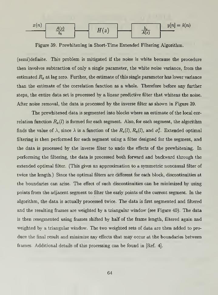
x(n)
boH(z)
y[n] = s(n)
A(z)
Figure 39. Prewhitening in Short-Time Extended Filtering Algorithm.
(semi) definite. This problem is mitigated if the noise is white because the procedure
then involves subtraction of only a single parameter, the white noise variance, from the
estimated Rx at lag zero. Further, the estimate of this single parameter has lower variance
than the estimate of the correlation function as a whole. Therefore before any further
steps, the entire data set is processed by a linear predictive filter that whitens the noise.
After noise removal, the data is processed by the inverse filter as shown in Figure 39.
The prewhitened data is segmented into blocks where an estimate of the local cor-
relation function RX {1) is formed for each segment. Also, for each segment, the algorithm
finds the value of A, since A is a function of the RS {1) ,^{l) , and of. Extended optimal
filtering is then performed for each segment using a filter designed for the segment, and
the data is processed by the inverse filter to undo the effects of the prewhitening. In
performing the filtering, the data is processed both forward and backward through the
extended optimal filter. (This gives an approximation to a symmetric noncausal filter of
twice the length.) Since the optimal filters are different for each block, discontinuities at
the boundaries can arise. The effect of such discontinuities can be minimized by using
points from the adjacent segment to filter the early points of the current segment. In the
algorithm, the data is actually processed twice. The data is first segmented and filtered
and the resulting frames are weighted by a triangular window (see Figure 40). The data
is then resegmented using frames shifted by half of the frame length, filtered again and
weighted by a triangular window. The two weighted sets of data are then added to pro-
duce the final result and minimize any effects that may occur at the boundaries between
frames. Additional details of this processing can be found in [Ref. 4].
64
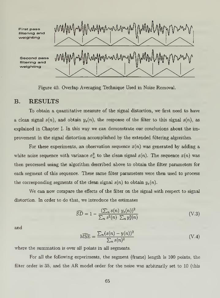
First passfiltering andweighting
Second Dassfiltering andweighting
Figure 40. Overlap Averaging Technique Used in Noise Removal.
B. RESULTSTo obtain a quantitative measure of the signal distortion, we first need to have
a clean signal s(n), and obtain ys (n), the response of the filter to this signal s(n), as
explained in Chapter I. In this way we can demonstrate our conclusions about the im-
provement in the signal distortion accomplished by the extended filtering algorithm.
For these experiments, an observation sequence x(ri) was generated by adding a
white noise sequence with variance a^ to the clean signal s(n). The sequence x{n) was
then processed using the algorithm described above to obtain the filter parameters for
each segment of this sequence. These same filter parameters were then used to process
the corresponding segments of the clean signal s(n) to obtain ys (n).
We can now compare the effects of the filter on the signal with respect to signal
distortion. In order to do that, we introduce the estimates
(£ns(n)t/s (n))2
and
SD = 1-
MSE =
E„s2 (n) En y2s(n)
En (S (n)-y(n)) 2
(V.3)
(V.4)EnS(n) 2
where the summation is over all points in all segments.
For all the following experiments, the segment (frame) length is 100 points, the
filter order is 35, and the AR model order for the noise was arbitrarily set to 10 (this
65
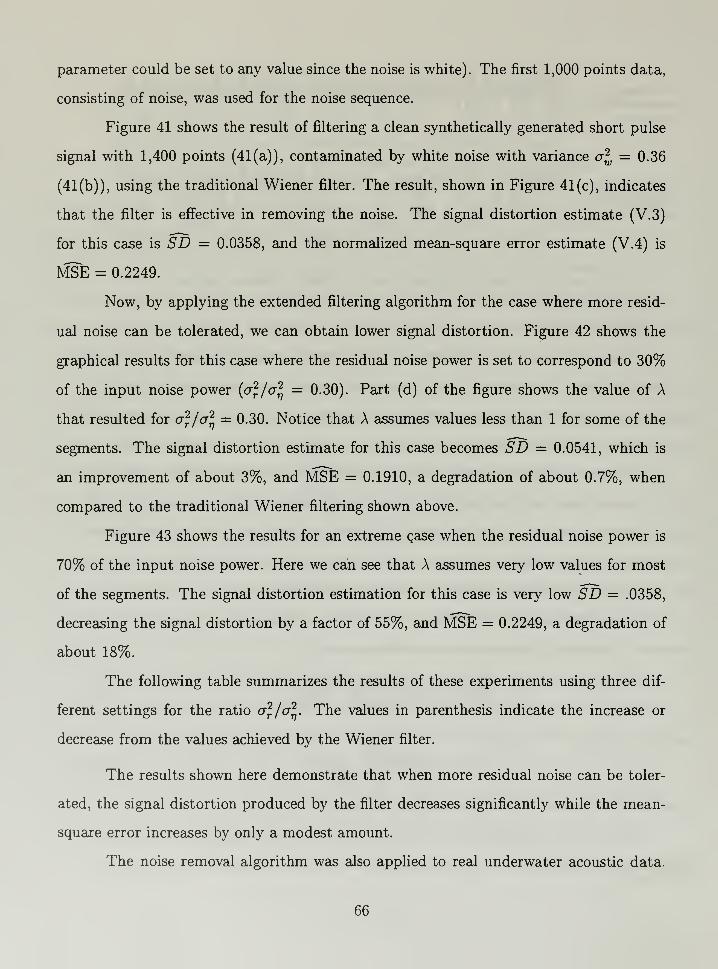
parameter could be set to any value since the noise is white). The first 1,000 points data,
consisting of noise, was used for the noise sequence.
Figure 41 shows the result of filtering a clean synthetically generated short pulse
signal with 1,400 points (41(a)), contaminated by white noise with variance cr^ = 0.36
(41(b)), using the traditional Wiener filter. The result, shown in Figure 41(c), indicates
that the filter is effective in removing the noise. The signal distortion estimate (V.3)
for this case is SD = 0.0358, and the normalized mean-square error estimate (V.4) is
MSE = 0.2249.
Now, by applying the extended filtering algorithm for the case where more resid-
ual noise can be tolerated, we can obtain lower signal distortion. Figure 42 shows the
graphical results for this case where the residual noise power is set to correspond to 30%
of the input noise power {a^/a^ = 0.30). Part (d) of the figure shows the value of A
that resulted for <7^/cr^ = 0.30. Notice that A assumes values less than 1 for some of the
segments. The signal distortion estimate for this case becomes SD = 0.0541, which is
an improvement of about 3%, and MSE = 0.1910, a degradation of about 0.7%, when
compared to the traditional Wiener filtering shown above.
Figure 43 shows the results for an extreme case when the residual noise power is
70% of the input noise power. Here we can see that A assumes very low values for most
of the segments. The signal distortion estimation for this case is very low SD = .0358,
decreasing the signal distortion by a factor of 55%, and MSE == 0.2249, a degradation of
about 18%.
The following table summarizes the results of these experiments using three dif-
ferent settings for the ratio of/c^. The values in parenthesis indicate the increase or
decrease from the values achieved by the Wiener filter.
The results shown here demonstrate that when more residual noise can be toler-
ated, the signal distortion produced by the filter decreases significantly while the mean-
square error increases by only a modest amount.
The noise removal algorithm was also applied to real underwater acoustic data.
66
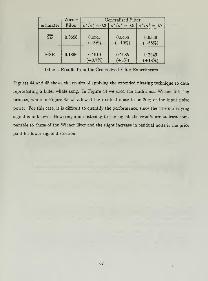
estimates
Wiener
Filter
Generalized Filter
<ZK = 0-3 ojfK = 0.5 &Uol = 0.7
SD 0.0556 0.0541
(-3%)
0.0466
(-19%)
0.0358
(-55%)
MSE 0.1896 0.1910
(+0.7%)
0.1985
(+5%)
0.2249
(+18%)
Table I. Results from the Generalized Filter Experiments.
Figures 44 and 45 shows the results of applying the extended filtering technique to data
representing a killer whale song. In Figure 44 we used the traditional Wiener filtering
process, while in Figure 45 we allowed the residual noise to be 20% of the input noise
power. For this case, it is difficult to quantify the performance, since the true underlying
signal is unknown. However, upon listening to the signal, the results are at least com-
parable to those of the Wiener filter and the slight increase in residual noise is the price
paid for lower signal distortion.
67
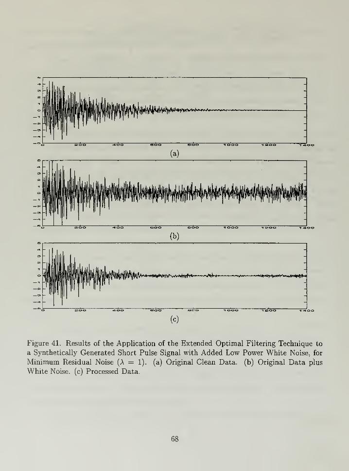
1 -«».oo
-i -o-oo
(b)
*4tvifT*" ' ^^,^>^^V^f' - «»/«»'. <>um.«»f^»Mn<yjvi»m^<t»^
(c)
Figure 41. Results of the Application of the Extended Optimal Filtering Technique to
a Synthetically Generated Short Pulse Signal with Added Low Power White Noise, for
Minimum Residual Noise (A = 1). (a) Original Clean Data, (b) Original Data plus
White Noise, (c) Processed Data.
68
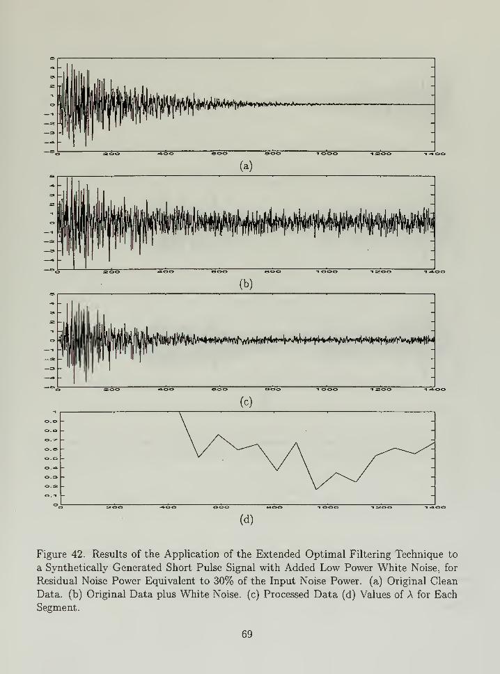
-i -*oo
-I -0.00
-1 soo -I "4-00
(d)
Figure 42. Results of the Application of the Extended Optimal Filtering Technique to
a Synthetically Generated Short Pulse Signal with Added Low Power White Noise, for
Residual Noise Power Equivalent to 30% of the Input Noise Power, (a) Original Clean
Data, (b) Original Data plus White Noise, (c) Processed Data (d) Values of A for Each
Segment.
69
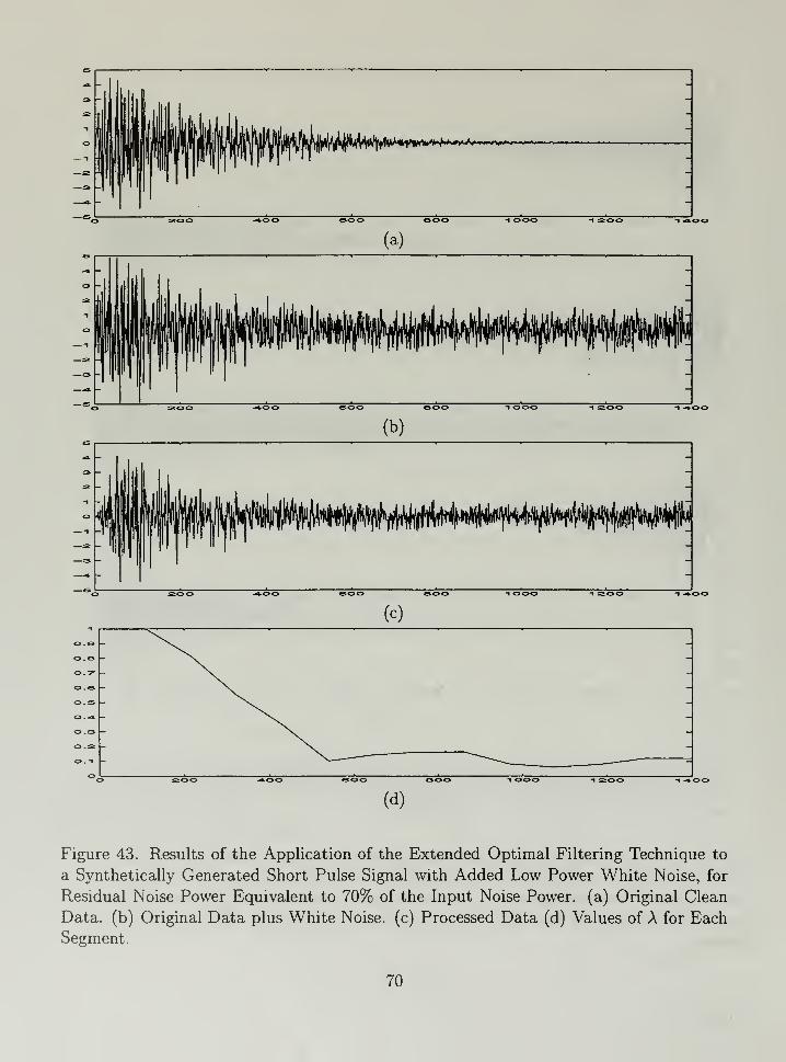
-% -»oo
T -*-00>
-I -l-OO
-1 soo
(d)
Figure 43. Results of the Application of the Extended Optimal Filtering Technique to
a Synthetically Generated Short Pulse Signal with Added Low Power White Noise, for
Residual Noise Power Equivalent to 70% of the Input Noise Power, (a) Original Clean
Data, (b) Original Data plus White Noise, (c) Processed Data (d) Values of A for Each
Segment.
70
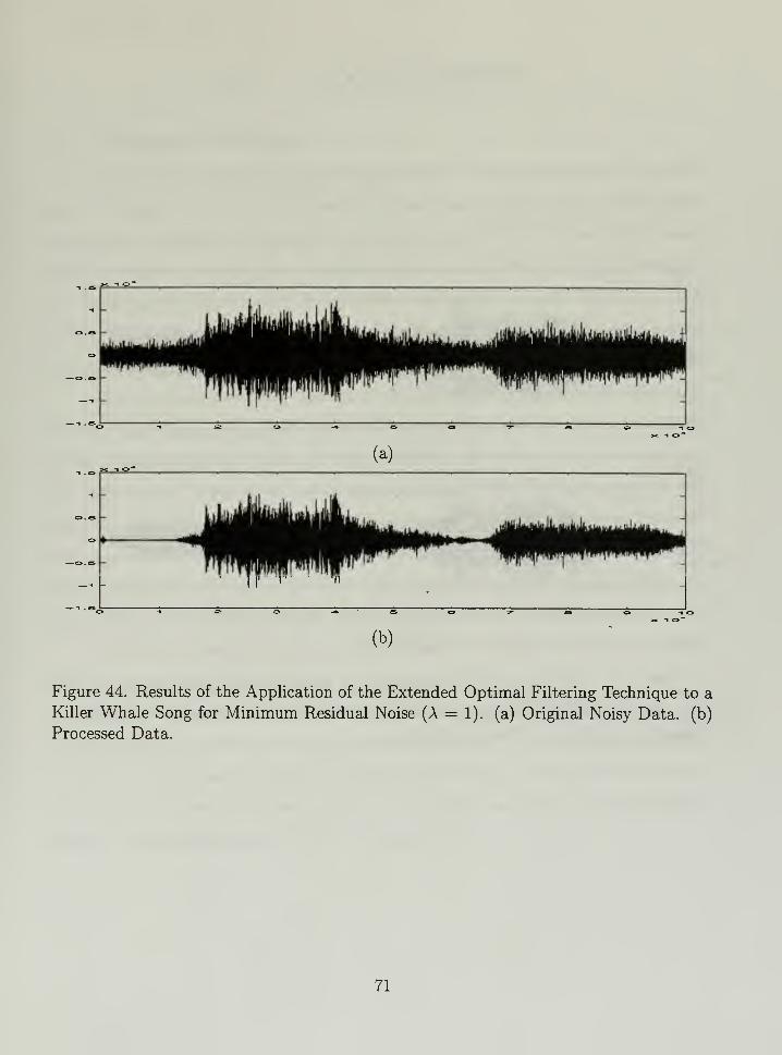
—o.es —
(a)
(b)
Figure 44. Results of the Application of the Extended Optimal Filtering Technique to a
Killer Whale Song for Minimum Residual Noise (A = 1). (a) Original Noisy Data, (b)
Processed Data.
71
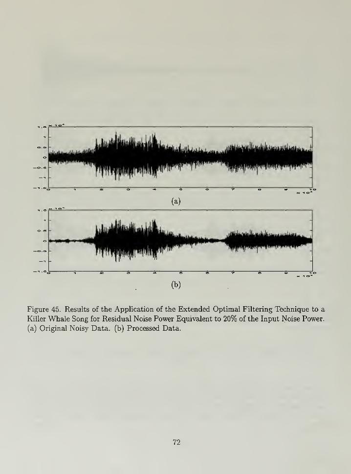
(a)
(b)
Figure 45. Results of the Application of the Extended Optimal Filtering Technique to a
Killer Whale Song for Residual Noise Power Equivalent to 20% of the Input Noise Power.
(a) Original Noisy Data, (b) Processed Data.
72
VI. CONCLUSIONS
A. THESIS SUMMARYThe first three chapters of this thesis provide an extensive analysis of the IIR
and FIR Wiener filters for removing additive noise from a desired signal. Both signal
and noise are represented by first order autoregressive (AR) models. Three performance
measures, namely processing gain, normalized mean-square error, and signal distortion
are defined and evaluated for the Wiener filters based on these models. We believe that
the behavior of these filters in terms of the defined performance measures is typical even
for other cases with more general signal and noise models.
It was seen that the FIR filter has performance similar to that of the IIR filter,
although it does not have the same ideal limiting characteristics such as infinite process-
ing gain when the signal becomes perfectly correlated. We also showed that while both
forms of the filter provide lower mean-square error and higher processing gain as the
signal becomes more correlated, signal distortion is not a monotonic function of correla-
tion. In particular the signal distortion for both forms of the filter peaks in a region of
moderately high correlation and increases when the input signal-to-noise ratio decreases.
This distortion introduced by the filter may be undesirable in some applications.
Chapters IV and V deal with a way to improve the signal distortion resulting
from the Wiener filter by considering a more general filtering problem. The result is
a generalized solution that can reduce the signal distortion of the Wiener filter, with
some increase in the mean-square error and residual noise. This solution was adopted
in a short-time filtering algorithm developed by Frack [Ref. 4] and tested. The results
illustrate that the extended filter provides more flexibility and allows more control over
the signal distortion introduced by the filtering process.
73
B. SUGGESTIONS FOR FUTURE RESEARCHThe results from this thesis can drive some further discussions, including the
performance of aural tests to evaluate the performance of the extended optimal filtering
technique when applied to real sonar data, and application to real-time signal processing.
In the time set aside to perform this thesis research the major portion of the effort
involved the analysis of the Wiener filter and its generalization. Relatively little time
was left for considering implementation details and more extensive testing on real data.
For more efficient implementation, the nonlinear equations that specify the parameter A
in terms of the residual noise a* need to be inverted more efficiently. This could be done
by a more effective iterative method or by inverting the function at a number of points
and performing table look-ups.
While the new algorithm is known to permit a trade-off in signal distortion versus
mean-square error, the practical effects of this trade-off have not been truly evaluated.
For example, formal listening tests have not been conducted to see (over some class
of signals) if listeners preferred the results of the generalized filter over those of the
conventional Wiener filter or, indeed, if they could hear the difference. The greatest
benefits may come in the use of this new algorithm in conjunction with further signal
processing steps which may be sensitive to any distortion of the signal introduced by the
noise removal process. These are all topics for possible future study.
74
LIST OF REFERENCES
[1] Urick, Robert J., Ambient Noise in the Sea, Peninsula Publishing, Los Altos, California,
1986.
[2] Machell, F. W., and C. S. Penrod, Probability Density Functions of Ocean Acoustic Noise
Processes. In E. J. Wegman and J. G. Smith, editors, Statistical Signal Processing. Marcel
Dekker, Inc., New York, 1984.
[3] Machell, F. W., C. S. Penrod, and G. E. Ellis. Statistical Characteristics of Ocean Acoustic
Noise Processes. In E. J. Wegman, S. C. Schwartz, and J. B. Thomas, editors, Topics in
Non-Gausian Signal Processing. Springer-Verlag, New York, New York, 1989.
[4] Frack, Kenneth L., Jr., "Improving Transient Signal Synthesis Through Noise Modeling and
Noise Removal", Master's Thesis, Naval Postgraduate School, Monterey, California, March1994.
[5] Therrien, Charles W., Discrete Random Signals and Statistical Signal Processing, Prentice
Hall, Inc., Englewood Cliffs, New Jersey, 1992.
[6] Wiener, Norbert, Extrapolation, Interpolation, and Smoothing of Stationary Time Series,
The M.I.T. Press (formerly Technology Press), Cambridge, Massachusetts, 1949. (Reprinted
as a paperback in 1964.).
[7] Ephraim, Yariv, and Harry L. Van Trees, A Signal Subspace Approach for Speech
Enhancement, IEEE Transactions on Speech and Audio Processing, 3(4):251-266, July
1995.
[8] Strang, Gilbert, Introduction to Applied Mathematics, Wellesley Cambridge Press,
Wellesley, Massachusetts, 1986.
75
76
INITIAL DISTRIBUTION LIST
1
.
Defense Technical Information Center 2
8725 John J. Kingman Road., Ste 0944
Ft. Belvoir, VA 22060-6218
2. Dudley Knox Library 2
Naval Postgraduate School
411 Dyer Rd.
Monterey, CA 93943-5101
3. Chairman, Code EC 1
Department of Electrical and Computer Engineering
Naval Postgraduate School
Monterey, CA 93943-5121
4. Prof. Charles W. Therrien, Code EC/Ti 3
Department of Electrical and Computer Engineering
Naval Postgraduate School
Monterey, CA 93943-5121
5. Prof. Anthony A. Atchley, Code PH/Ay 1
Physics Department
Naval Postgraduate School
Monterey, CA 93943-5121
6. Prof. Monique Fargues, Code EC/Fa 1
Department of Electrical and Computer Engineering
Naval Postgraduate School
Monterey, CA 93943-5121
7. Mr. Steve Greineder, Code 2121 2
NUWC DIVPT1176 Howel Street
Newport, RI 02841-1708
8. LCDR Natanael Ruiz Fontes, 3
Brazilian Naval Commission
5130 MacArthur Blvd., N.W.
Washington, DC, 20016-3344
77

OXUBRARY-TGRADUATE SCHOOL,'CA '"""'^ioi

DUDLEY KNOX LIBRARY
3 2768 00339477 6


