An empirical approach to investigate the relationship between Overall Equipment Effectiveness and Energy consumptions: an application in the manufacturing field

An empirical approach to investigate the relationship between Overall Equipment Effectiveness

and Energy consumptions: an application in the manufacturing field

Vittorio Cesarotti*, Vito Introna*, Raffaele Rotunno**, Giulia Scerrato**

* Department of Enterprise Engineering, University of Rome “Tor Vergata”, Via del Politecnico 1, 00133 Rome ‐ Italy ([email protected], [email protected])

** Department of Industrial Engineering, University of Rome “Tor Vergata”, Via del Politecnico 1, 00133 Rome ‐ Italy ([email protected], [email protected])

Abstract:

In the last decades energy efficiency of production systems has become a key concern in several industry fields, due to the increased energy costs and the associated environmental impacts. Furthermore, the role of equipment efficiency has lately occupied a relevant place, due to the importance of equipment performances in an optimized system. The fundamental aspect is that the two dimensions are strictly related, and it is possible to better understand complex systems by deeply comprehending this connection.

Purpose

With these assumption, in this paper the authors want to investigate through the analysis of a real manufacturing process how the OEE-related loss have an impact on equipment energy consumptions.

Design/methodology/approach

Present work will be structured in two phases: an analysis step, in which by comparing energy values and trends, for systems in different operative conditions, it is possible to investigate how energy consumption varies; and a modeling step where the relationship between OEE and energy efficiency is observed in their relevant ranges, to verify the hypothesis and validate the model.

The model variables will be the single OEE loss as it is logical to assume that a non-efficient equipment requires a higher quantity of energy, for instance being close to its failure modes, or operating at non-optimal conditions. Also, it is clear the relevance of high defects rate, as the time lost to produce non-valuable products requires a certain amount of energy which will not be repaid.

Originality/value

Previous researches investigated on the key performance indicators (KPIs) to correlate energy efficiency of machineries and production while they do not examine in depth the relation between increased productivity index (OEE) and energy savings related to it. The study will be significant for industrial companies, as it allows to strictly relate the energy usage to its causes and to improve both energy and efficiency aspects. Indeed, from the efficiency point of view, energy consumption can represent specific problems symptoms that, if correctly identified, can be specifically attacked and resolved. In return, by improving the efficiency levels of the equipments, the whole energy consumptions will be lowered, obtaining considerable cost reductions and environmental benefits. This will represent a first step of study, to be developed with more detailed and complex cases and situations, analyzing extended data quantities and structuring appropriate simulative models.

Keywords: “Energy Efficiency”, “OEE”, “Energy Consumption”, “Productivity”, “Environment”.

1. Introduction

It is well known that our future depends on a sustainable development: as a consequence, during the last decades, the focus is on the quantification of the carbon footprint and demand for future reductions. This trend is supported by the increase in energy cost and the progressive depletion of non-renewable resources.

Manufacturers are responsible for around fifty percent of commercial energy usage (World Energy Outlook 2011) and almost the same percentage of greenhouse gases.

As a result, many industries have already put in place a lot of actions related to reduction in consumption of energy and carbon dioxide emissions including: switch-off campaigns, scheduling production when energy charges are at their lowest, replacing tools and machinery with more energy-efficient units, using automatic system to turn devices off and a greater control on leaks.

All of these actions are capital for a continuous improvement in energy management but they are not enough on their own.

There is a further step forward to be made represented by operating the factory as efficiently as possible in order to maximise energy efficiency: breakdowns, set-up and adjustment loss, minor stoppage, slow running equipment, rejects and reduced yield all have a direct relationship with energy usage.

According to these considerations, purpose of the paper is twofold:

• to demonstrate that OEE-related loss does not only affect plant efficiency but have also a major impact on energy consumption;

• to investigate how the relation between the two dimensions changes according to different variables and conditions involved.

The analysis will be performed by studying a real productive unit, observing its behaviour when subjected to efficiency losses, related to:

• Availability factors, such as equipment failure, set-up and adjustment;

• Performance factors, as idling, minor stops and reduced speed;

• Quality factors due to defects in process, start-up losses, etc.

Through this approach it will be possible to quantify the effect of inefficiency not only in terms of OEE productivity index, but even in terms of energy usage.

For example, a bottleneck which breaks down, or which is running slowly, has not only impact in term of productivity reduction, but it has an impact in consumption of energy too. As a matter of fact, in-feeding tools and machinery, as well as out-feeding equipment, are kept powered up even during the downtime, so that there is a large amount of energy which result wasted without control. As consequence, optimizing bottlenecks OEE

efficiency, not only will result in an increment of productivity, but will impact directly in a reduction of energy consumption as well.

2. Energy Management

2.1 Background

Over the next years, energy demand is expected to rise impacting adversely to the cost of providing customers with energy (Gorke F. et all, 2005).

Consequently, energy concerns are becoming key factors and drivers for economic development in the industrial field, forasmuch as the weight they have in the overall production cost.

The use of renewable sources is a long term solution but, in the short-run, the adoption of an energy efficiency politic is necessary to reduce both cost and noxious emissions.

As specified by the standard ISO 50001:2011, Energy management systems – Requirements with guidance for use), in order to enable an organization to achieve a continuous improvement of energy performance, an energy management system is to be implemented.

The principle on which this system is based is the continuous monitoring of energy and environmental performance by bounding the consumption to each activity or resource (Cesarotti and Introna, 2010).

The optimization of productive processes is the main tool to support an organization’s competitive advantage; as a consequence, the attention to energy efficiency continued to grow vigorously in the last years (Carminati, et al., 2008).

Previous researches investigated on the key performance indicators (KPIs) to correlate energy consumption and production while they do not examine in depth the relation between increased productivity and energy savings related to it.

Present study analyzes the effect of improved energy efficiency through the optimization of productivity comparing it to the effect of technical energy efficiency measures on devices.

2.2 Industrial insight

The level of commitment to the reduction in energy consumption depends on the production reality: process manufacturing plants, whose energy costs are a large amount of total costs, are more energy efficiency sensitive than small manufacturing companies. Overall, energy consumption is due to specific productive processes and auxiliary facilities (i.e HVAC: heating, ventilation, air conditioning). Costs allocation between these categories can significantly change but, broadly, energy intensive organizations incur in higher cost to support the productive process itself. On the other hand, in manufacturing companies in particular, the auxiliary

facilities are the responsible for the major part of the total energy costs.

Implementing an energy management system allows to significantly reduce production costs, making the saved resources available for new and more business-oriented investments.

Furthermore, energy control is closely linked to a reduction in the emission of pollutants and CO2, allowing in some cases to prevent fines linked with the stringent emission limits.

Focusing, in this paper, specifically on industrial processes we can say that energy efficiency is never constant over time; accordingly, understanding the cause-and-effect relationships between the internal and external variables affecting it, is therefore a prerequisite for the management of energy consumption in day-to-day operations. The following ratio expresses the energy efficiency (Patterson, 1996):

𝐸𝑛𝑒𝑟𝑔𝑦𝐸𝑓𝑓𝑖𝑐𝑖𝑒𝑛𝑐𝑦 =

𝑈𝑠𝑒𝑓𝑢𝑙 𝑜𝑢𝑡𝑝𝑢𝑡 𝑜𝑓 𝑎 𝑝𝑟𝑜𝑐𝑒𝑠𝑠𝐸𝑛𝑒𝑟𝑔𝑦 𝑝𝑢𝑡 𝑖𝑛𝑡𝑜 𝑎 𝑝𝑟𝑜𝑐𝑒𝑠𝑠

There are several energy saving initiatives to reduce consumption impact on production cost but it is possible to identify two complementary approaches:

• Increasing the energy efficiency of equipment (concerns reduction of energy consumption and includes the substitution of devices – or part of them, with more energy efficient ones);

• Increasing the productivity efficiency of the equipment (monitoring and improving the OEE to identify and correct the occurred losses).

Generally, the majority of the initiatives undertaken to reduce energy consumption are focused on saving energy by improving the technical efficiency of utilities and devices (i.e. power factor correction interventions, variable speed drive compressor, etc.).

Nevertheless, while such energy efficiency solutions can guarantee significant saving by operating on equipment nameplate capacity, additional energy conservation can be attained by optimizing the overall production of the process.

In fact, factors responsible for production inefficiency also affect negatively energy consumptions.

A high rate of reject pieces that do not meet quality standards, inefficient production scheduling, slow running equipment, are all clear examples of energy waste causes.

Therefore, focusing solely on savings achievable by increasing machineries energy efficiency (or on energy conservation) has a limited room for improvement if the opportunities of productivity index optimization are not taken into account.

3. Discussion

In the majority of manufacturing processes we can observe, in a period, a linear dependence between the total consumption of energy and production volume:

𝐸 = 𝐸0 + 𝛼 ∙ 𝑉

Where:

• E is the total consumption of energy in a defined period;

• E0 is the standard energy consumed by the process irrespective of the level of production (i.e. electric heating, engines always on, etc.);

• 𝛼 is a coefficient which expresses the theoretical incremental energy consumed for the production of one additional unit of output;

• V is the production volume.

The simplest and most valuable measure of energy efficiency achievements in a manufacturing plant is unit consumption, or energy used per unit produced. Unit consumption provides the best indicator of how effectively the energy consumed by a plant is being put into use, and can be tracked over time to measure energy efficiency improvements (Gallachóir and Cahill, 2009).

Consequently, as production increases, the fix cost due to E0 can be shared on a larger quantity of output and then, energy efficiency is enhanced.

In addition, it is important to notice that, assuming the case of constant loading time, the production volume varies depending on the OEE index, a metric to measure how effectively a system is utilized. As OEE increase more output are produced for less resource in the considered period; then it also influences the energy efficiency of the system.

Finally, it is to notice that although if OEE is the same the production level is equal, the energy consumption can vary depending on the type of loss (it can differ if the diminution of the index is due to setup, slow running equipment or breakdowns).

This close dependency makes necessary the monitoring over time of energy consumption and OEE; in fact the study of their relation may allow to:

• Obtain and keep the best performances of the system;

• Consider the energy saving achievable by the improvement of OEE beyond the other benefit from reducing the production losses;

• Distinguish between the increase of unit consumption due to planned efficiency losses (i.e. setup, predictive maintenance stops) and avoidable losses (or containable by an early intervention, for instance in case of recurring breakdown).

The continuous control of energy consumption and cost can be performed by statistical tools already used in other

sectors as control charts or CUSUM chart (Cesarotti, Introna, 2009).

In particular, CUSUM chart shows the cumulative differences between successive values (actual consumption over a period of time) and target values (standard consumption), useful at identifying variation in performance and saving/waste incurred to date.

3.1 Relation between OEE and Energy Efficiency

As stated beforehand, OEE impacts on total energy consumption since as production volume increases per-unit fixed costs get lower because these costs are shared over a larger number of units.

Conversely, what is not immediately evident is how each different type of loss can influence energy efficiency.

According to Nakajima (1988) OEE is expressed as a percentage, and calculated by the following formula:

𝑂𝐸𝐸 = 𝐴𝑣𝑎𝑖𝑙𝑎𝑏𝑖𝑙𝑖𝑡𝑦 ∙ 𝑃𝑒𝑟𝑓𝑜𝑟𝑚𝑎𝑛𝑐𝑒 ∙ 𝑄𝑢𝑎𝑙𝑖𝑡𝑦

Each factor is related to different time loss, generated by different causes:

• Availability (A), refers to the percentage of Scheduled time actually capitalized, once removed all the time loss due to equipment macro-stoppages (it consists of breakdown and downtime losses, setup losses and start-up losses). Further in the document we refer to those time loss as LTIME;

• Performance (Ep), refers to the percentage of Operative time actually capitalized, once removed all the time loss due to equipment micro stoppages or lack of speed (it includes minor stoppages, slow running equipment and slowing down in start-up losses). Further in the document we refer to those time loss as LSPEED;

• Quality (Q), refers to the percentage of Net Operative Time actually capitalized, once removed all the time loss due to working activities to process non-sellable units (production rejects) or to rework micro-defected units (rework quality losses). Further in the document we refer to those time loss as LQUAL.

Each of these type of loss results in energy waste basing on the workings described below:

• Breakdown and downtime losses. Caused by machine faults, unplanned production stops because of maintenance and waiting times – apart from the broken equipment, most of the plant; conveyors, pumps, shrink tunnels, etc. continue to cycle, use more energy to get back up to speed than standard running.

In addition, it is important to underline that when an equipment is close to a breakage point, it may consume more energy than when it operates in normal conditions (e.g. additional friction within the components). Also, when two or more machines are

strictly connected, or if the stoppage lasts for an extended amount of time, the effect of the downtime influence all of those other devices as well (since they cannot produce and are left in stand-bye). For what concern the aims of this paper, since the attention is posed on standalone equipment only, these last terms will not be included in the analytical formulation. .

𝐸𝑛𝑒𝑟𝑔𝑦𝐵𝐷 = 𝑇𝑖𝑚𝑒𝑀𝐴𝐿𝐹𝑈𝑁𝐶𝑇𝐼𝑂𝑁 ∙ 𝑃𝑜𝑤𝑒𝑟𝑁𝐸𝐸𝐷 .

• Setup losses. Caused by setting up of a line, retooling or product changeover. .

𝐸𝑛𝑒𝑟𝑔𝑦𝑆𝑈𝑃 = � #𝑆𝐸𝑇𝑈𝑃 𝑖 ∙ 𝑃𝑜𝑤𝑒𝑟𝑁𝐸𝐸𝐷 𝑖 ∙ 𝑇𝑖𝑚𝑒𝑆𝐸𝑇𝑈𝑃 𝑖𝑖

. In both these first two cases, if power required by equipment tends to zero there are only production efficiency losses but there is no impact on energy efficiency.

Consequently, when these types of losses occur, actions to assure minimum power to equipment should put in place (i.e. auto-switching off of devices).

• Start-up losses. Most machineries of industrial processes use more energy at start-up than at normal operating speed, particularly electricity, so if the plant breaks down frequently more energy will be used. .

𝐸𝑛𝑒𝑟𝑔𝑦𝑆𝑇𝐴𝑅𝑇 = #𝑆𝑊𝐼𝑇𝐶𝐻 ∙ 𝑇𝑖𝑚𝑒𝑆𝑊𝐼𝑇𝐶𝐻 ∙ 𝑃𝑜𝑤𝑒𝑟𝑁𝐸𝐸𝐷 .

• Minor stoppages losses. Caused by temporary malfunction, hindered product flow or short-lasting idle times – consume as much energy as machineries working at the ideal speed. They have the same functioning of macro stoppages losses but, being minor switching off actions are not to be applied, contrary to the other case (it is not worthwhile to stop a device for a micro stoppage considering the consequent start-up process).

• Slow running equipment losses. In terms of energy efficiency the impact of a slowing down depends on the specific production process. In fact machinery speed can, or not, influence energy consumption and it is necessary to analyse case by case.

• Slowing down in start-up losses. This is a kind of loss linked to the phase before the device go full speed. As in the precedent case, the impact on energy consumption depends on the specific production process.

• Production rejects losses. Scrap materials use as much energy as good outputs: .

𝐸𝑛𝑒𝑟𝑔𝑦𝑅𝐸𝐽𝐸𝐶𝑇𝑆 = #𝑅𝐸𝐽𝐸𝐶𝑇𝑆 ∙ 𝑇𝑖𝑚𝑒𝑃𝑅𝑂𝐷𝑈𝐶𝑇𝐼𝑂𝑁 ∙ 𝑃𝑜𝑤𝑒𝑟𝑁𝐸𝐸𝐷 .

• Rework quality losses. Compared to reject losses, the energy used to produce a product that do not meet

quality specification is not completely waste because there is the opportunity to rework it. Obviously it costs more, also in terms of energy, than a good product. .

𝐸𝑛𝑒𝑟𝑔𝑦𝑅𝐸𝑊𝑂𝑅𝐾𝑆 = #𝑅𝐸𝑊𝑂𝑅𝐾𝑆 ∙ 𝑇𝑖𝑚𝑒𝑃𝑅𝑂𝐷 ∙ 𝑃𝑜𝑤𝑒𝑟𝑁𝐸𝐸𝐷

+ #𝑅𝐸𝑊𝑂𝑅𝐾𝑆 ∙ 𝑇𝑖𝑚𝑒𝑅𝐸𝑊𝑂𝑅𝐾 ∙ 𝑃𝑜𝑤𝑒𝑟𝑅𝐸𝑊𝑂𝑅𝐾 . All these losses lead equipment to have an under-utilized capacity as well as higher energy consumptions. Industries often invest in additional capacity, unaware that increasing the OEE index of current underperforming lines may provide the increase in production they desire. In addition, the outlined relationship bring up another significant consideration about the importance of improve OEE factor, rather than invest in additional resources. An adequate equipment management helps reduce energy wastes as well, contributing to develop more sustainable solution, while introducing additional-not-needed resources leads towards the opposite direction.

3.2.1 Case study

In this section we show the inter-relationship between OEE and energy through a case study in a manufacturing organization specialized in packaging operations. Results indicate that lower production efficiency has a direct impact both on productivity and energy cost.

3.2.1.1 About the organization

The plant considered in our case study produces a wide range of products, different by type and size (for instance aluminium lid and chest, polypropylene food trays, etc.) and it is divided in two main operation department: aluminium and plastic. The ABC analysis conducted in the organization has revealed that the highest cost is related to the provision of electricity.

The majority of equipment are resistance heating machines used to warm production process inputs in order to expedite their manufacturing. They essentially work at constant temperature of 45°C and absorb active energy. All the other devices (e.g. mills and shredders) impact on reactive energy.

Data collection was performed through a monitoring system of instantaneous power, installed on each machine. Communication of data between the sender device and the receiving computer is realized by wireless technology. Software receives the data and averages out each 15 minutes. The output is a time chart showing several measures as average power, absorbed energy, active and reactive energy and total production.

Absorbed energy/total production ratio provides us with some valuable insight into the energy consumption over the process.

Obviously, the desideratum is an energy consumption as low as possible: this would indicate that the system is

efficiently and effectively working and the process is correctly planned.

All the data used to perform our analysis refer to energy consumption per work shift, for the production of different types of products. For the scope of this paper, data have been considered as related to the production of a single type of product (there are minimum approximations, as showed in other analysis).

3.2.1.2 Data analysis

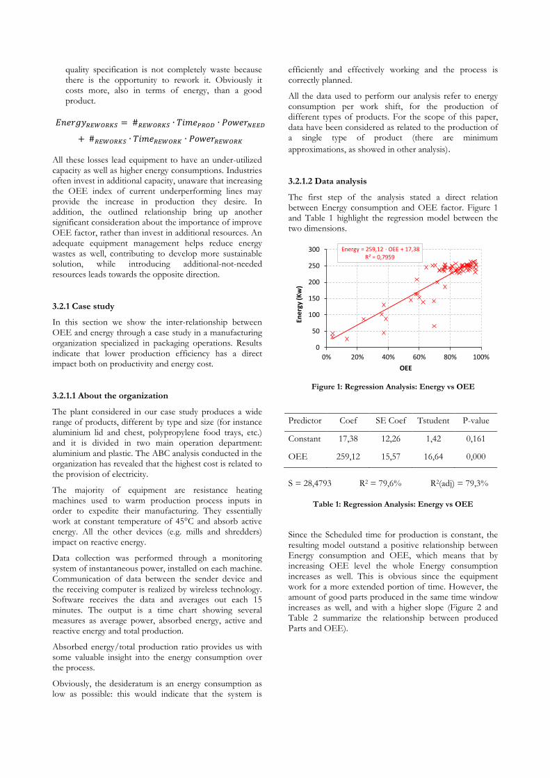
The first step of the analysis stated a direct relation between Energy consumption and OEE factor. Figure 1 and Table 1 highlight the regression model between the two dimensions.

Figure 1: Regression Analysis: Energy vs OEE

Predictor Coef SE Coef Tstudent P-value

Constant 17,38 12,26 1,42 0,161

OEE 259,12 15,57 16,64 0,000

S = 28,4793 R2 = 79,6% R2(adj) = 79,3%

Table 1: Regression Analysis: Energy vs OEE

Since the Scheduled time for production is constant, the resulting model outstand a positive relationship between Energy consumption and OEE, which means that by increasing OEE level the whole Energy consumption increases as well. This is obvious since the equipment work for a more extended portion of time. However, the amount of good parts produced in the same time window increases as well, and with a higher slope (Figure 2 and Table 2 summarize the relationship between produced Parts and OEE).

Energy = 259,12 ∙ OEE + 17,38 R² = 0,7959

0

50

100

150

200

250

300

0% 20% 40% 60% 80% 100%

Ener

gy (K

w)

OEE

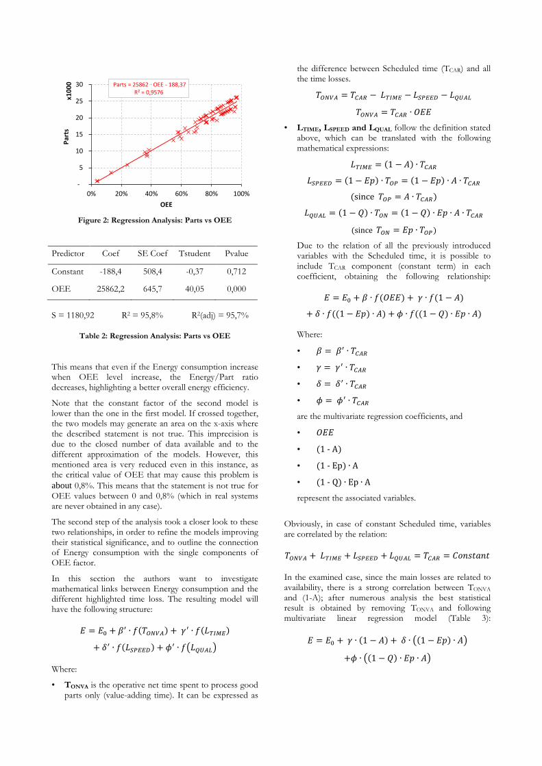
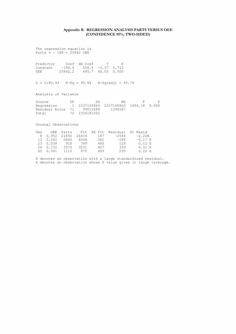
Figure 2: Regression Analysis: Parts vs OEE

Predictor Coef SE Coef Tstudent Pvalue

Constant -188,4 508,4 -0,37 0,712

OEE 25862,2 645,7 40,05 0,000

S = 1180,92 R2 = 95,8% R2(adj) = 95,7%

Table 2: Regression Analysis: Parts vs OEE

This means that even if the Energy consumption increase when OEE level increase, the Energy/Part ratio decreases, highlighting a better overall energy efficiency.

Note that the constant factor of the second model is lower than the one in the first model. If crossed together, the two models may generate an area on the x-axis where the described statement is not true. This imprecision is due to the closed number of data available and to the different approximation of the models. However, this mentioned area is very reduced even in this instance, as the critical value of OEE that may cause this problem is about 0,8%. This means that the statement is not true for OEE values between 0 and 0,8% (which in real systems are never obtained in any case).

The second step of the analysis took a closer look to these two relationships, in order to refine the models improving their statistical significance, and to outline the connection of Energy consumption with the single components of OEE factor.

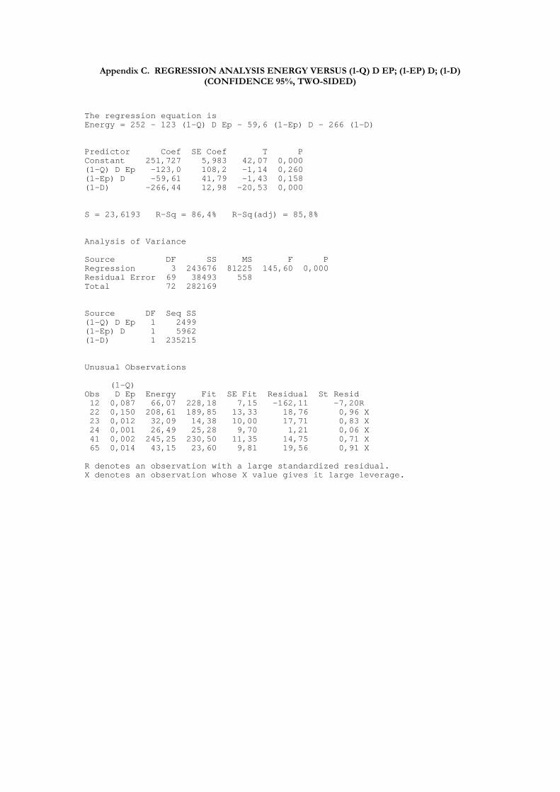
In this section the authors want to investigate mathematical links between Energy consumption and the different highlighted time loss. The resulting model will have the following structure: .

𝐸 = 𝐸0 + 𝛽′ ∙ 𝑓(𝑇𝑂𝑁𝑉𝐴) + 𝛾′ ∙ 𝑓(𝐿𝑇𝐼𝑀𝐸)

+ 𝛿′ ∙ 𝑓(𝐿𝑆𝑃𝐸𝐸𝐷) + 𝜙′ ∙ 𝑓�𝐿𝑄𝑈𝐴𝐿� . Where:

• TONVA is the operative net time spent to process good parts only (value-adding time). It can be expressed as

the difference between Scheduled time (TCAR) and all the time losses.

𝑇𝑂𝑁𝑉𝐴 = 𝑇𝐶𝐴𝑅 − 𝐿𝑇𝐼𝑀𝐸 − 𝐿𝑆𝑃𝐸𝐸𝐷 − 𝐿𝑄𝑈𝐴𝐿

𝑇𝑂𝑁𝑉𝐴 = 𝑇𝐶𝐴𝑅 ∙ 𝑂𝐸𝐸

• LTIME, LSPEED and LQUAL follow the definition stated above, which can be translated with the following mathematical expressions:

𝐿𝑇𝐼𝑀𝐸 = (1 − 𝐴) ∙ 𝑇𝐶𝐴𝑅

𝐿𝑆𝑃𝐸𝐸𝐷 = (1 − 𝐸𝑝) ∙ 𝑇𝑂𝑃 = (1 − 𝐸𝑝) ∙ 𝐴 ∙ 𝑇𝐶𝐴𝑅

(since 𝑇𝑂𝑃 = 𝐴 ∙ 𝑇𝐶𝐴𝑅)

𝐿𝑄𝑈𝐴𝐿 = (1 − 𝑄) ∙ 𝑇𝑂𝑁 = (1 − 𝑄) ∙ 𝐸𝑝 ∙ 𝐴 ∙ 𝑇𝐶𝐴𝑅

(since 𝑇𝑂𝑁 = 𝐸𝑝 ∙ 𝑇𝑂𝑃) Due to the relation of all the previously introduced variables with the Scheduled time, it is possible to include TCAR component (constant term) in each coefficient, obtaining the following relationship: .

𝐸 = 𝐸0 + 𝛽 ∙ 𝑓(𝑂𝐸𝐸) + 𝛾 ∙ 𝑓(1 − 𝐴)

+ 𝛿 ∙ 𝑓((1 − 𝐸𝑝) ∙ 𝐴) + 𝜙 ∙ 𝑓((1 − 𝑄) ∙ 𝐸𝑝 ∙ 𝐴) . Where:

• 𝛽 = 𝛽′ ∙ 𝑇𝐶𝐴𝑅

• 𝛾 = 𝛾′ ∙ 𝑇𝐶𝐴𝑅

• 𝛿 = 𝛿′ ∙ 𝑇𝐶𝐴𝑅

• 𝜙 = 𝜙′ ∙ 𝑇𝐶𝐴𝑅

are the multivariate regression coefficients, and

• 𝑂𝐸𝐸

• (1 ‐ A)

• (1 ‐ Ep) ∙ A

• (1 ‐ Q) ∙ Ep ∙ A

represent the associated variables.

Obviously, in case of constant Scheduled time, variables are correlated by the relation: .

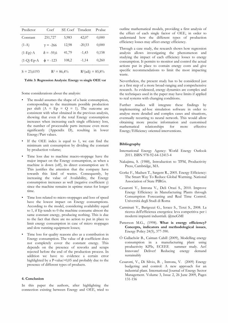
𝑇𝑂𝑁𝑉𝐴 + 𝐿𝑇𝐼𝑀𝐸 + 𝐿𝑆𝑃𝐸𝐸𝐷 + 𝐿𝑄𝑈𝐴𝐿 = 𝑇𝐶𝐴𝑅 = 𝐶𝑜𝑛𝑠𝑡𝑎𝑛𝑡 . In the examined case, since the main losses are related to availability, there is a strong correlation between TONVA and (1-A); after numerous analysis the best statistical result is obtained by removing TONVA and following multivariate linear regression model (Table 3): .

𝐸 = 𝐸0 + 𝛾 ∙ (1 − 𝐴) + 𝛿 ∙ �(1 − 𝐸𝑝) ∙ 𝐴�

+𝜙 ∙ �(1 − 𝑄) ∙ 𝐸𝑝 ∙ 𝐴�

Parts = 25862 ∙ OEE - 188,37 R² = 0,9576

-

5

10

15

20

25

30

0% 20% 40% 60% 80% 100%

Part

s x1

000

OEE

Predictor Coef SE Coef Tstudent Pvalue

Constant 251,727 5,983 42,07 0,000

(1-A) γ = -266 12,98 -20,53 0,000

(1-Ep)∙A δ = -59,6 41,79 -1,43 0,158

(1-Q)∙Ep∙A ϕ = -123 108,2 -1,14 0,260

S = 23,6193 R2 = 86,4% R2(adj) = 85,8%

Table 3: Regression Analysis: Energy vs single OEE var

Some considerations about the analysis: • The model assumes the shape of a basic consumption,

corresponding to the maximum possible production per shift (A = Ep = Q = 1). The outcome are consistent with what obtained in the previous analysis, showing that even if the total Energy consumption increases when increasing each single efficiency loss, the number of processable parts increase even more significantly (Appendix D), resulting in lower Energy/Part values.

• If the OEE index is equal to 1, we can find the minimum unit consumption by dividing the constant by production volume;

• Time loss due to machine macro-stoppage have the major impact on the Energy consumption, as when a machine is down (off), its direct consumption are 0. This justifies the attention that the company have towards this kind of wastes. Consequently, by increasing the value of Availability, the Energy consumption increases as well (negative coefficient γ) since the machine remains in uptime status for longer time.

• Time loss related to micro-stoppages and loss of speed have the lowest impact on Energy consumptions. According to the model, considering availability equal to 1, if Ep tends to 0 the machine consume almost the same constant energy, producing nothing. This is due to the fact that there are no action to put in place to limit energy consumption in case of micro stoppages and slow running equipment losses;

• Time loss for quality reasons also as a contribution in Energy consumption. The value of 𝜙 coefficient does not completely cover the constant energy. This depends on the presence of reworks and scraps rejected before the end of the production process. In addition we have to evidence a certain error highlighted by a P-value>0,05 and probably due to the presence of different types of products.

4. Conclusion

In this paper the authors, after highlighting the connection existing between Energy and OEE, tried to

outline mathematical models, providing a first analysis of the effect of each single factor of OEE, in order to understand how the different types of production efficiency losses may affect energy efficiency.

Through a case study, the research shows how regression analysis allows investigating the phenomenon and studying the impact of each efficiency losses to energy consumption. It permits to monitor and control the actual actions put in place to contain energy costs and give specific recommendations to limit the most impacting waste.

Nevertheless, the present study has to be considered just as a first step of a more broad-ranging and comprehensive research. As evidenced, energy dynamics are complex and the techniques used in the paper may have limits if applied to real systems with changing conditions.

Further studies will integrate these findings by implementing ad-hoc simulation software in order to analyse more detailed and complex cases and situations, eventually recurring to neural network. This would allow obtaining more precise information and customised mathematical relationships for more effective Energy/Efficiency oriented interventions.

Bibliography

International Energy Agency: World Energy Outlook 2011. ISBN 978-92-64-12413-4

Nakajima, S. (1988), Introduction to TPM, Productivity Press, Cambridge, MA.

Gorke F., Madsen T., Sargent R., 2005. Energy Efficiency: The Smart Way To Reduce Global Warming. National Association of State PIRGs.

Cesarotti V., Introna V., Deli Orazi S., 2010. Improve Energy Efficiency in Manufacturing Plants through Consumption Forecasting and Real Time Control. Università degli Studi di Roma

Carminati V., Barigozzi G., Ierace S., Terzi S., 2008. La ricerca dell'efficienza energetica: leva competitiva per i moderni impianti industriali. @meGMI

Patterson M.G., (1998). What is energy efficiency? Concepts, indicators and methodological issues, Energy Policy 24(5), 377-390.

Ó Gallachóir B., Caiman Cahill (2009), Modelling energy consumption in a manufacturing plant using productivity KPIs, ECEEE summer study. Act! Innovate! Deliver! Reducing energy demand sustainably

Cesarotti, V., Di Silvio, B. , Introna, V. (2009) Energy budgeting and control: A new approach for an industrial plant. International Journal of Energy Sector Management. Volume 3, Issue 2, 26 June 2009, Pages 131-156

Appendix A. REGRESSION ANALYSIS ENERGY VERSUS OEE (CONFIDENCE 95%, TWO-SIDED)

The regression equation isEnergy = 17,4 + 259 OEE

Predictor Coef SE Coef T PConstant 17,38 12,26 1,42 0,161OEE 259,12 15,57 16,64 0,000

S = 28,4793 R-Sq = 79,6% R-Sq(adj) = 79,3%

Analysis of Variance

Source DF SS MS F PRegression 1 224583 224583 276,90 0,000Residual Error 71 57586 811Total 72 282169

Unusual Observations

Obs OEE Energy Fit SE Fit Residual St Resid 9 0,371 45,11 113,51 6,88 -68,40 -2,48R12 0,697 66,07 198,09 3,46 -132,02 -4,67R13 0,241 86,79 79,87 8,71 6,92 0,26 X23 0,038 32,09 27,17 11,70 4,92 0,19 X24 0,132 26,49 51,64 10,29 -25,15 -0,95 X41 0,646 245,25 184,80 3,76 60,46 2,14R65 0,041 43,15 28,03 11,65 15,12 0,58 X

R denotes an observation with a large standardized residual.X denotes an observation whose X value gives it large leverage.

Appendix B. REGRESSION ANALYSIS PARTS VERSUS OEE (CONFIDENCE 95%, TWO-SIDED)

The regression equation isParts = - 188 + 25862 OEE

Predictor Coef SE Coef T PConstant -188,4 508,4 -0,37 0,712OEE 25862,2 645,7 40,05 0,000

S = 1180,93 R-Sq = 95,8% R-Sq(adj) = 95,7%




Obs OEE Parts Fit SE Fit Residual St Resid 8 0,952 21850 24434 187 -2584 -2,22R13 0,241 5860 6048 361 -188 -0,17 X23 0,038 918 789 485 129 0,12 X24 0,132 3570 3231 427 339 0,31 X65 0,041 1110 875 483 235 0,22 X


Appendix C. REGRESSION ANALYSIS ENERGY VERSUS (1-Q) D EP; (1-EP) D; (1-D) (CONFIDENCE 95%, TWO-SIDED)

The regression equation isEnergy = 252 - 123 (1-Q) D Ep - 59,6 (1-Ep) D - 266 (1-D)

Predictor Coef SE Coef T PConstant 251,727 5,983 42,07 0,000(1-Q) D Ep -123,0 108,2 -1,14 0,260(1-Ep) D -59,61 41,79 -1,43 0,158(1-D) -266,44 12,98 -20,53 0,000

S = 23,6193 R-Sq = 86,4% R-Sq(adj) = 85,8%



Source DF Seq SS(1-Q) D Ep 1 2499(1-Ep) D 1 5962(1-D) 1 235215


(1-Q)Obs D Ep Energy Fit SE Fit Residual St Resid12 0,087 66,07 228,18 7,15 -162,11 -7,20R22 0,150 208,61 189,85 13,33 18,76 0,96 X23 0,012 32,09 14,38 10,00 17,71 0,83 X24 0,001 26,49 25,28 9,70 1,21 0,06 X41 0,002 245,25 230,50 11,35 14,75 0,71 X65 0,014 43,15 23,60 9,81 19,56 0,91 X


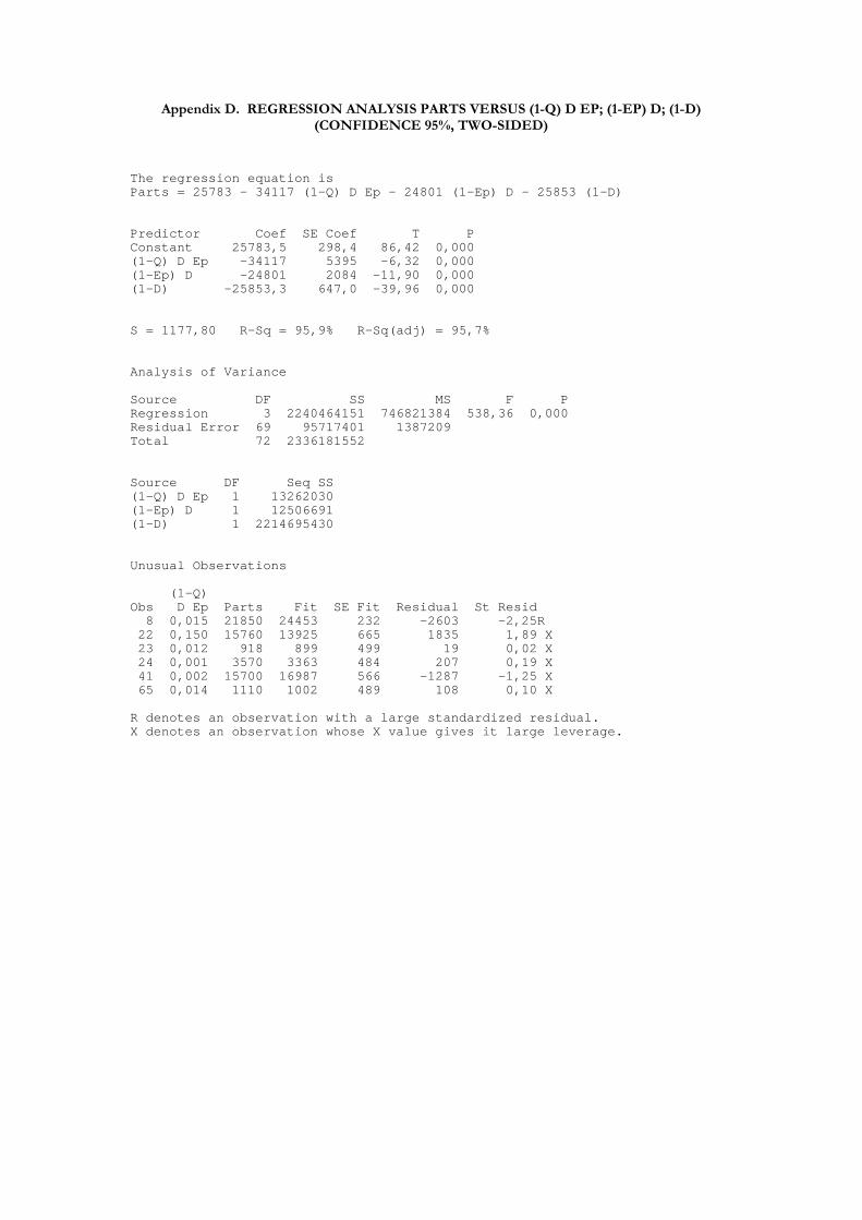
Appendix D. REGRESSION ANALYSIS PARTS VERSUS (1-Q) D EP; (1-EP) D; (1-D) (CONFIDENCE 95%, TWO-SIDED)

The regression equation isParts = 25783 - 34117 (1-Q) D Ep - 24801 (1-Ep) D - 25853 (1-D)

Predictor Coef SE Coef T PConstant 25783,5 298,4 86,42 0,000(1-Q) D Ep -34117 5395 -6,32 0,000(1-Ep) D -24801 2084 -11,90 0,000(1-D) -25853,3 647,0 -39,96 0,000

S = 1177,80 R-Sq = 95,9% R-Sq(adj) = 95,7%



Source DF Seq SS(1-Q) D Ep 1 13262030(1-Ep) D 1 12506691(1-D) 1 2214695430


(1-Q)Obs D Ep Parts Fit SE Fit Residual St Resid 8 0,015 21850 24453 232 -2603 -2,25R22 0,150 15760 13925 665 1835 1,89 X23 0,012 918 899 499 19 0,02 X24 0,001 3570 3363 484 207 0,19 X41 0,002 15700 16987 566 -1287 -1,25 X65 0,014 1110 1002 489 108 0,10 X


Documents

An empirical approach to investigate the relationship between Overall Equipment Effectiveness and Energy consumptions: an application in the manufacturing field