CDM Homework Problems

Klaus Sutnerhttp://www.cs.cmu.edu/˜sutner

c© 2002–2019

Contents

1 Logic 101.1 Converting Xor (50) . . . . . . . . . . . . . . . . . . . . . . . . . . . . . . . . . . . . . . . . . . . . . . 111.2 Math Profs (50) . . . . . . . . . . . . . . . . . . . . . . . . . . . . . . . . . . . . . . . . . . . . . . . . . 121.3 Hats (50) . . . . . . . . . . . . . . . . . . . . . . . . . . . . . . . . . . . . . . . . . . . . . . . . . . . . 131.4 Proof Patterns (50) . . . . . . . . . . . . . . . . . . . . . . . . . . . . . . . . . . . . . . . . . . . . . . . 141.5 Irrationality (50) . . . . . . . . . . . . . . . . . . . . . . . . . . . . . . . . . . . . . . . . . . . . . . . . 151.6 Circle Divisions (50) . . . . . . . . . . . . . . . . . . . . . . . . . . . . . . . . . . . . . . . . . . . . . . 161.7 Infinitude of Primes (50) . . . . . . . . . . . . . . . . . . . . . . . . . . . . . . . . . . . . . . . . . . . . 171.8 True/False/Random (50) . . . . . . . . . . . . . . . . . . . . . . . . . . . . . . . . . . . . . . . . . . . 181.9 Magic Words (50) . . . . . . . . . . . . . . . . . . . . . . . . . . . . . . . . . . . . . . . . . . . . . . . 191.10 Syllogisms (50) . . . . . . . . . . . . . . . . . . . . . . . . . . . . . . . . . . . . . . . . . . . . . . . . . 201.11 Boolean Set Operations (50) . . . . . . . . . . . . . . . . . . . . . . . . . . . . . . . . . . . . . . . . . . 211.12 Finsler (50) . . . . . . . . . . . . . . . . . . . . . . . . . . . . . . . . . . . . . . . . . . . . . . . . . . . 221.13 Sums and Products (50) . . . . . . . . . . . . . . . . . . . . . . . . . . . . . . . . . . . . . . . . . . . . 231.14 Tautology Testing (50) . . . . . . . . . . . . . . . . . . . . . . . . . . . . . . . . . . . . . . . . . . . . . 241.15 Normal Forms (50) . . . . . . . . . . . . . . . . . . . . . . . . . . . . . . . . . . . . . . . . . . . . . . . 251.16 DNF (50) . . . . . . . . . . . . . . . . . . . . . . . . . . . . . . . . . . . . . . . . . . . . . . . . . . . . 261.17 Dual Formulae (20) . . . . . . . . . . . . . . . . . . . . . . . . . . . . . . . . . . . . . . . . . . . . . . . 271.18 Biconditionals (50) . . . . . . . . . . . . . . . . . . . . . . . . . . . . . . . . . . . . . . . . . . . . . . . 281.19 Biconditionals (50) . . . . . . . . . . . . . . . . . . . . . . . . . . . . . . . . . . . . . . . . . . . . . . . 291.20 Symmetric Differences (50) . . . . . . . . . . . . . . . . . . . . . . . . . . . . . . . . . . . . . . . . . . 301.21 UnEqual Satisfiability (50) . . . . . . . . . . . . . . . . . . . . . . . . . . . . . . . . . . . . . . . . . . . 311.22 Davis-Putnam (50) . . . . . . . . . . . . . . . . . . . . . . . . . . . . . . . . . . . . . . . . . . . . . . . 321.23 Quantifiers (50) . . . . . . . . . . . . . . . . . . . . . . . . . . . . . . . . . . . . . . . . . . . . . . . . . 331.24 Predicate Badgers (50) . . . . . . . . . . . . . . . . . . . . . . . . . . . . . . . . . . . . . . . . . . . . . 341.25 Verifying Frege (50) . . . . . . . . . . . . . . . . . . . . . . . . . . . . . . . . . . . . . . . . . . . . . . 351.26 Natural Deduction (50) . . . . . . . . . . . . . . . . . . . . . . . . . . . . . . . . . . . . . . . . . . . . 361.27 Natural Deduction in Predicate Logic (50) . . . . . . . . . . . . . . . . . . . . . . . . . . . . . . . . . . 371.28 Maximally Consistent Sets (50) . . . . . . . . . . . . . . . . . . . . . . . . . . . . . . . . . . . . . . . . 381.29 One Unary Function (50) . . . . . . . . . . . . . . . . . . . . . . . . . . . . . . . . . . . . . . . . . . . 391.30 Formulae over Q and R (50) . . . . . . . . . . . . . . . . . . . . . . . . . . . . . . . . . . . . . . . . . . 401.31 Graphs and FOL (30) . . . . . . . . . . . . . . . . . . . . . . . . . . . . . . . . . . . . . . . . . . . . . 41

1

1.32 Presburger and Skolem Arithmetic (40) . . . . . . . . . . . . . . . . . . . . . . . . . . . . . . . . . . . 421.33 Weak Arithmetic (50) . . . . . . . . . . . . . . . . . . . . . . . . . . . . . . . . . . . . . . . . . . . . . 431.34 Pierce Arithmetic (50) . . . . . . . . . . . . . . . . . . . . . . . . . . . . . . . . . . . . . . . . . . . . . 441.35 Peano Arithmetic (50) . . . . . . . . . . . . . . . . . . . . . . . . . . . . . . . . . . . . . . . . . . . . . 451.36 Interpolation (50) . . . . . . . . . . . . . . . . . . . . . . . . . . . . . . . . . . . . . . . . . . . . . . . . 461.37 Unary and Binary (50) . . . . . . . . . . . . . . . . . . . . . . . . . . . . . . . . . . . . . . . . . . . . . 471.38 Maps and Powersets (50) . . . . . . . . . . . . . . . . . . . . . . . . . . . . . . . . . . . . . . . . . . . 481.39 Dedekind Infinity (50) . . . . . . . . . . . . . . . . . . . . . . . . . . . . . . . . . . . . . . . . . . . . . 491.40 Functions as Relations (50) . . . . . . . . . . . . . . . . . . . . . . . . . . . . . . . . . . . . . . . . . . 501.41 Transitivity and Ordinals (50) . . . . . . . . . . . . . . . . . . . . . . . . . . . . . . . . . . . . . . . . . 511.42 Universal Relations (50) . . . . . . . . . . . . . . . . . . . . . . . . . . . . . . . . . . . . . . . . . . . . 521.43 Order Completion (50) . . . . . . . . . . . . . . . . . . . . . . . . . . . . . . . . . . . . . . . . . . . . . 531.44 Pairs (50) . . . . . . . . . . . . . . . . . . . . . . . . . . . . . . . . . . . . . . . . . . . . . . . . . . . . 541.45 Antisymmetry (10) . . . . . . . . . . . . . . . . . . . . . . . . . . . . . . . . . . . . . . . . . . . . . . . 551.46 Transitivity (10) . . . . . . . . . . . . . . . . . . . . . . . . . . . . . . . . . . . . . . . . . . . . . . . . 56

2 Computation 572.1 Some Graph Problems (40) . . . . . . . . . . . . . . . . . . . . . . . . . . . . . . . . . . . . . . . . . . 582.2 Fixed Point to Recursion Theorem (30) . . . . . . . . . . . . . . . . . . . . . . . . . . . . . . . . . . . 592.3 Historical Ackermann (30) . . . . . . . . . . . . . . . . . . . . . . . . . . . . . . . . . . . . . . . . . . . 602.4 Lists via Coding (30) . . . . . . . . . . . . . . . . . . . . . . . . . . . . . . . . . . . . . . . . . . . . . . 612.5 Node Deletion (20) . . . . . . . . . . . . . . . . . . . . . . . . . . . . . . . . . . . . . . . . . . . . . . . 622.6 Sat Oracle (20) . . . . . . . . . . . . . . . . . . . . . . . . . . . . . . . . . . . . . . . . . . . . . . . . . 632.7 Arithmetizing Branching Programs (30) . . . . . . . . . . . . . . . . . . . . . . . . . . . . . . . . . . . 642.8 Branching Programs and BPP (30) . . . . . . . . . . . . . . . . . . . . . . . . . . . . . . . . . . . . . . 652.9 Paths and Trees (30) . . . . . . . . . . . . . . . . . . . . . . . . . . . . . . . . . . . . . . . . . . . . . . 662.10 Easy SAT Versions (30) . . . . . . . . . . . . . . . . . . . . . . . . . . . . . . . . . . . . . . . . . . . . 672.11 Tilings (40) . . . . . . . . . . . . . . . . . . . . . . . . . . . . . . . . . . . . . . . . . . . . . . . . . . . 682.12 More Tilings (20) . . . . . . . . . . . . . . . . . . . . . . . . . . . . . . . . . . . . . . . . . . . . . . . . 692.13 Simulating Space (20) . . . . . . . . . . . . . . . . . . . . . . . . . . . . . . . . . . . . . . . . . . . . . 702.14 Medians (20) . . . . . . . . . . . . . . . . . . . . . . . . . . . . . . . . . . . . . . . . . . . . . . . . . . 712.15 Regular Expression Equivalence (40) . . . . . . . . . . . . . . . . . . . . . . . . . . . . . . . . . . . . . 722.16 Immerman-Szelepsenyi (20) . . . . . . . . . . . . . . . . . . . . . . . . . . . . . . . . . . . . . . . . . . 732.17 Graphs and NL (20) . . . . . . . . . . . . . . . . . . . . . . . . . . . . . . . . . . . . . . . . . . . . . . 742.18 Small Space (20) . . . . . . . . . . . . . . . . . . . . . . . . . . . . . . . . . . . . . . . . . . . . . . . . 752.19 Computing Log-Space Functions (40) . . . . . . . . . . . . . . . . . . . . . . . . . . . . . . . . . . . . . 762.20 SAT Versions (30) . . . . . . . . . . . . . . . . . . . . . . . . . . . . . . . . . . . . . . . . . . . . . . . 772.21 Subset Sum (30) . . . . . . . . . . . . . . . . . . . . . . . . . . . . . . . . . . . . . . . . . . . . . . . . 782.22 BDDs (40) . . . . . . . . . . . . . . . . . . . . . . . . . . . . . . . . . . . . . . . . . . . . . . . . . . . . 792.23 Linear Time Reductions (25) . . . . . . . . . . . . . . . . . . . . . . . . . . . . . . . . . . . . . . . . . 802.24 Pretty Colors (25) . . . . . . . . . . . . . . . . . . . . . . . . . . . . . . . . . . . . . . . . . . . . . . . 812.25 Kleene Star (25) . . . . . . . . . . . . . . . . . . . . . . . . . . . . . . . . . . . . . . . . . . . . . . . . 82

2

2.26 Minimization Problems (25) . . . . . . . . . . . . . . . . . . . . . . . . . . . . . . . . . . . . . . . . . . 832.27 Classification in AH (40) . . . . . . . . . . . . . . . . . . . . . . . . . . . . . . . . . . . . . . . . . . . . 842.28 Decidability and Proofs (60) . . . . . . . . . . . . . . . . . . . . . . . . . . . . . . . . . . . . . . . . . . 852.29 Classifying Index Sets (20) . . . . . . . . . . . . . . . . . . . . . . . . . . . . . . . . . . . . . . . . . . . 862.30 Decidability and Computable Functions (40) . . . . . . . . . . . . . . . . . . . . . . . . . . . . . . . . 872.31 Minimal Machines (30) . . . . . . . . . . . . . . . . . . . . . . . . . . . . . . . . . . . . . . . . . . . . . 882.32 Primitive Recursive Word Functions (40) . . . . . . . . . . . . . . . . . . . . . . . . . . . . . . . . . . 892.33 Kolmogorov versus Palindromes (50) . . . . . . . . . . . . . . . . . . . . . . . . . . . . . . . . . . . . . 902.34 Kolmogorov versus Primes (30) . . . . . . . . . . . . . . . . . . . . . . . . . . . . . . . . . . . . . . . . 912.35 Degrees and Reductions (50) . . . . . . . . . . . . . . . . . . . . . . . . . . . . . . . . . . . . . . . . . 922.36 Iteration and Diagonals (30) . . . . . . . . . . . . . . . . . . . . . . . . . . . . . . . . . . . . . . . . . . 932.37 RMs and Binary Digit Sums (30) . . . . . . . . . . . . . . . . . . . . . . . . . . . . . . . . . . . . . . . 942.38 Sequence Numbers (20) . . . . . . . . . . . . . . . . . . . . . . . . . . . . . . . . . . . . . . . . . . . . 952.39 Length and Sequence Numbers (30) . . . . . . . . . . . . . . . . . . . . . . . . . . . . . . . . . . . . . 962.40 Register Machines and Sequence Numbers (50) . . . . . . . . . . . . . . . . . . . . . . . . . . . . . . . 972.41 Loopy Loops (40) . . . . . . . . . . . . . . . . . . . . . . . . . . . . . . . . . . . . . . . . . . . . . . . . 982.42 Shallow Loop Programs (50) . . . . . . . . . . . . . . . . . . . . . . . . . . . . . . . . . . . . . . . . . 992.43 Some Primitive Recursive Functions (20) . . . . . . . . . . . . . . . . . . . . . . . . . . . . . . . . . . . 1002.44 Course-of-Value Recursion (20) . . . . . . . . . . . . . . . . . . . . . . . . . . . . . . . . . . . . . . . . 1012.45 The Busy Beaver Function (RM) (30) . . . . . . . . . . . . . . . . . . . . . . . . . . . . . . . . . . . . 1022.46 The Busy Beaver Function (TM) (50) . . . . . . . . . . . . . . . . . . . . . . . . . . . . . . . . . . . . 1032.47 The Busy Beaver Function (Programs) (40) . . . . . . . . . . . . . . . . . . . . . . . . . . . . . . . . . 1042.48 Overhead-Free Automata (40) . . . . . . . . . . . . . . . . . . . . . . . . . . . . . . . . . . . . . . . . . 1052.49 Teleporting Turing Machines (20) . . . . . . . . . . . . . . . . . . . . . . . . . . . . . . . . . . . . . . . 1062.50 Write-First Turing Machines (20) . . . . . . . . . . . . . . . . . . . . . . . . . . . . . . . . . . . . . . . 1072.51 Binary Register Machines (30) . . . . . . . . . . . . . . . . . . . . . . . . . . . . . . . . . . . . . . . . 1082.52 Reduced Turing Machines (40) . . . . . . . . . . . . . . . . . . . . . . . . . . . . . . . . . . . . . . . . 1092.53 Semi-Decidable Sets and Computable Functions (40) . . . . . . . . . . . . . . . . . . . . . . . . . . . . 1102.54 Semi-Decidable Sets and Computable Functions (80) . . . . . . . . . . . . . . . . . . . . . . . . . . . . 1112.55 Graphs of Computable Functions (40) . . . . . . . . . . . . . . . . . . . . . . . . . . . . . . . . . . . . 1122.56 Oracles (20) . . . . . . . . . . . . . . . . . . . . . . . . . . . . . . . . . . . . . . . . . . . . . . . . . . . 1132.57 Vertex Cover and SAT (50) . . . . . . . . . . . . . . . . . . . . . . . . . . . . . . . . . . . . . . . . . . 1142.58 Easy Satisfiability (50) . . . . . . . . . . . . . . . . . . . . . . . . . . . . . . . . . . . . . . . . . . . . . 1152.59 Partition (25) . . . . . . . . . . . . . . . . . . . . . . . . . . . . . . . . . . . . . . . . . . . . . . . . . . 1162.60 Adding Numbers (30) . . . . . . . . . . . . . . . . . . . . . . . . . . . . . . . . . . . . . . . . . . . . . 1172.61 Kolmogorov Complexity (20) . . . . . . . . . . . . . . . . . . . . . . . . . . . . . . . . . . . . . . . . . 1182.62 Uninspired Sets (50) . . . . . . . . . . . . . . . . . . . . . . . . . . . . . . . . . . . . . . . . . . . . . . 1192.63 Expressiveness of FOL (20) . . . . . . . . . . . . . . . . . . . . . . . . . . . . . . . . . . . . . . . . . . 1202.64 Two 2-Tag Systems (30) . . . . . . . . . . . . . . . . . . . . . . . . . . . . . . . . . . . . . . . . . . . . 1212.65 Post Tag Systems (30) . . . . . . . . . . . . . . . . . . . . . . . . . . . . . . . . . . . . . . . . . . . . . 122

3 Induction, Iteration 124

3

3.1 Inflationary Functions (50) . . . . . . . . . . . . . . . . . . . . . . . . . . . . . . . . . . . . . . . . . . 1253.2 Noetherian Induction (50) . . . . . . . . . . . . . . . . . . . . . . . . . . . . . . . . . . . . . . . . . . . 1263.3 Divisibility (50) . . . . . . . . . . . . . . . . . . . . . . . . . . . . . . . . . . . . . . . . . . . . . . . . . 1273.4 Counting Digits (50) . . . . . . . . . . . . . . . . . . . . . . . . . . . . . . . . . . . . . . . . . . . . . . 1283.5 m-Leaders (50) . . . . . . . . . . . . . . . . . . . . . . . . . . . . . . . . . . . . . . . . . . . . . . . . . 1293.6 Inflationary Functions (50) . . . . . . . . . . . . . . . . . . . . . . . . . . . . . . . . . . . . . . . . . . 1303.7 Spreading Negativity (50) . . . . . . . . . . . . . . . . . . . . . . . . . . . . . . . . . . . . . . . . . . . 1313.8 Hereditarily Finite Sets (50) . . . . . . . . . . . . . . . . . . . . . . . . . . . . . . . . . . . . . . . . . . 1323.9 Inverse Sequences (50) . . . . . . . . . . . . . . . . . . . . . . . . . . . . . . . . . . . . . . . . . . . . . 1333.10 Mystery Recursion (50) . . . . . . . . . . . . . . . . . . . . . . . . . . . . . . . . . . . . . . . . . . . . 1343.11 Nested Recursion (50) . . . . . . . . . . . . . . . . . . . . . . . . . . . . . . . . . . . . . . . . . . . . . 1363.12 Powers of Two (50) . . . . . . . . . . . . . . . . . . . . . . . . . . . . . . . . . . . . . . . . . . . . . . . 1373.13 Collapsing Transformations (50) . . . . . . . . . . . . . . . . . . . . . . . . . . . . . . . . . . . . . . . 1383.14 Reversal and Palindromes (50) . . . . . . . . . . . . . . . . . . . . . . . . . . . . . . . . . . . . . . . . 1393.15 Lookup Tables and Iteration (50) . . . . . . . . . . . . . . . . . . . . . . . . . . . . . . . . . . . . . . . 1403.16 Iteration and Composites (50) . . . . . . . . . . . . . . . . . . . . . . . . . . . . . . . . . . . . . . . . . 1413.17 Fast Exponentiation (50) . . . . . . . . . . . . . . . . . . . . . . . . . . . . . . . . . . . . . . . . . . . 1423.18 Greatest Common Divisor (50) . . . . . . . . . . . . . . . . . . . . . . . . . . . . . . . . . . . . . . . . 1433.19 Binary Square Roots (50) . . . . . . . . . . . . . . . . . . . . . . . . . . . . . . . . . . . . . . . . . . . 1443.20 The Josephus Problem (50) . . . . . . . . . . . . . . . . . . . . . . . . . . . . . . . . . . . . . . . . . . 1453.21 Thue and Shuffle (25) . . . . . . . . . . . . . . . . . . . . . . . . . . . . . . . . . . . . . . . . . . . . . 1463.22 Fibonacci Words (25) . . . . . . . . . . . . . . . . . . . . . . . . . . . . . . . . . . . . . . . . . . . . . 1473.23 Mycielski Graphs (25) . . . . . . . . . . . . . . . . . . . . . . . . . . . . . . . . . . . . . . . . . . . . . 1483.24 Tournaments and Kings (25) . . . . . . . . . . . . . . . . . . . . . . . . . . . . . . . . . . . . . . . . . 1493.25 Tournaments and Fairness (25) . . . . . . . . . . . . . . . . . . . . . . . . . . . . . . . . . . . . . . . . 1503.26 Ducci Sequences (50) . . . . . . . . . . . . . . . . . . . . . . . . . . . . . . . . . . . . . . . . . . . . . . 1513.27 The DAZS Operator (60) . . . . . . . . . . . . . . . . . . . . . . . . . . . . . . . . . . . . . . . . . . . 1523.28 UnCollatz (50) . . . . . . . . . . . . . . . . . . . . . . . . . . . . . . . . . . . . . . . . . . . . . . . . . 1543.29 Son of Collatz (50) . . . . . . . . . . . . . . . . . . . . . . . . . . . . . . . . . . . . . . . . . . . . . . . 1553.30 Floyd on Steroids (20) . . . . . . . . . . . . . . . . . . . . . . . . . . . . . . . . . . . . . . . . . . . . . 1563.31 Floyd and Teleportation (50) . . . . . . . . . . . . . . . . . . . . . . . . . . . . . . . . . . . . . . . . . 1573.32 Schroder-Bernstein (50) . . . . . . . . . . . . . . . . . . . . . . . . . . . . . . . . . . . . . . . . . . . . 1583.33 Cardinalities (50) . . . . . . . . . . . . . . . . . . . . . . . . . . . . . . . . . . . . . . . . . . . . . . . . 1593.34 Frontiers of Trees (10) . . . . . . . . . . . . . . . . . . . . . . . . . . . . . . . . . . . . . . . . . . . . . 1603.35 An Iteration (50) . . . . . . . . . . . . . . . . . . . . . . . . . . . . . . . . . . . . . . . . . . . . . . . . 1613.36 Coinduction (50) . . . . . . . . . . . . . . . . . . . . . . . . . . . . . . . . . . . . . . . . . . . . . . . . 163

4 Algebra 1654.1 Indecomposable Matrices (50) . . . . . . . . . . . . . . . . . . . . . . . . . . . . . . . . . . . . . . . . . 1664.2 Rotations (50) . . . . . . . . . . . . . . . . . . . . . . . . . . . . . . . . . . . . . . . . . . . . . . . . . 1674.3 Rotating Words (50) . . . . . . . . . . . . . . . . . . . . . . . . . . . . . . . . . . . . . . . . . . . . . . 1684.4 Subgroups and Counting (50) . . . . . . . . . . . . . . . . . . . . . . . . . . . . . . . . . . . . . . . . . 169

4

4.5 Matrix Products (50) . . . . . . . . . . . . . . . . . . . . . . . . . . . . . . . . . . . . . . . . . . . . . . 1704.6 Fibonacci Monoid (50) . . . . . . . . . . . . . . . . . . . . . . . . . . . . . . . . . . . . . . . . . . . . . 1714.7 Affine Maps (50) . . . . . . . . . . . . . . . . . . . . . . . . . . . . . . . . . . . . . . . . . . . . . . . . 1724.8 Normal Subgroups (50) . . . . . . . . . . . . . . . . . . . . . . . . . . . . . . . . . . . . . . . . . . . . 1734.9 Modular Multiplication (50) . . . . . . . . . . . . . . . . . . . . . . . . . . . . . . . . . . . . . . . . . . 1744.10 Iterating Quadratic Residues (50) . . . . . . . . . . . . . . . . . . . . . . . . . . . . . . . . . . . . . . . 1754.11 An Associative Operation (50) . . . . . . . . . . . . . . . . . . . . . . . . . . . . . . . . . . . . . . . . 1764.12 Generating Permutations and Functions (50) . . . . . . . . . . . . . . . . . . . . . . . . . . . . . . . . 1774.13 Matrices and Words (50) . . . . . . . . . . . . . . . . . . . . . . . . . . . . . . . . . . . . . . . . . . . . 1784.14 Some Boolean Formulas (30) . . . . . . . . . . . . . . . . . . . . . . . . . . . . . . . . . . . . . . . . . 1794.15 Boolean Rings (50) . . . . . . . . . . . . . . . . . . . . . . . . . . . . . . . . . . . . . . . . . . . . . . . 1804.16 Boolean Algebras and Duality (50) . . . . . . . . . . . . . . . . . . . . . . . . . . . . . . . . . . . . . . 1814.17 Boolean Algebras (30) . . . . . . . . . . . . . . . . . . . . . . . . . . . . . . . . . . . . . . . . . . . . . 1824.18 Boolean Algebras without Times (50) . . . . . . . . . . . . . . . . . . . . . . . . . . . . . . . . . . . . 1834.19 A Transformation Semigroup (30) . . . . . . . . . . . . . . . . . . . . . . . . . . . . . . . . . . . . . . 1844.20 Floyd goes Algebraic (50) . . . . . . . . . . . . . . . . . . . . . . . . . . . . . . . . . . . . . . . . . . . 1854.21 Polynomial Equations Mod 2 (25) . . . . . . . . . . . . . . . . . . . . . . . . . . . . . . . . . . . . . . 1864.22 Functions versus Polynomials (30) . . . . . . . . . . . . . . . . . . . . . . . . . . . . . . . . . . . . . . 1874.23 Functions versus Polynomials (30) . . . . . . . . . . . . . . . . . . . . . . . . . . . . . . . . . . . . . . 1884.24 Chessboards and Lights (40) . . . . . . . . . . . . . . . . . . . . . . . . . . . . . . . . . . . . . . . . . 1894.25 Shrinking Dimension (20) . . . . . . . . . . . . . . . . . . . . . . . . . . . . . . . . . . . . . . . . . . . 1914.26 Building A Finite Field (20) . . . . . . . . . . . . . . . . . . . . . . . . . . . . . . . . . . . . . . . . . . 1924.27 Moving Cubes (50) . . . . . . . . . . . . . . . . . . . . . . . . . . . . . . . . . . . . . . . . . . . . . . . 1934.28 Grid Actions (50) . . . . . . . . . . . . . . . . . . . . . . . . . . . . . . . . . . . . . . . . . . . . . . . . 1944.29 Characteristic 2 (50) . . . . . . . . . . . . . . . . . . . . . . . . . . . . . . . . . . . . . . . . . . . . . . 1954.30 Redundant Field Representations (50) . . . . . . . . . . . . . . . . . . . . . . . . . . . . . . . . . . . . 196

5 Combinatorics 1975.1 Fast Fibonacci (50) . . . . . . . . . . . . . . . . . . . . . . . . . . . . . . . . . . . . . . . . . . . . . . . 1985.2 Pairing Sequences (50) . . . . . . . . . . . . . . . . . . . . . . . . . . . . . . . . . . . . . . . . . . . . . 1995.3 Self-Organizing Search (10) . . . . . . . . . . . . . . . . . . . . . . . . . . . . . . . . . . . . . . . . . . 2005.4 Comparisons in Randomized Quicksort (10) . . . . . . . . . . . . . . . . . . . . . . . . . . . . . . . . . 2015.5 Shooting Blanks (10) . . . . . . . . . . . . . . . . . . . . . . . . . . . . . . . . . . . . . . . . . . . . . . 2025.6 Vanilla Search Trees (10) . . . . . . . . . . . . . . . . . . . . . . . . . . . . . . . . . . . . . . . . . . . 2035.7 From Real to Binary (10) . . . . . . . . . . . . . . . . . . . . . . . . . . . . . . . . . . . . . . . . . . . 2045.8 Shifty Columns (10) . . . . . . . . . . . . . . . . . . . . . . . . . . . . . . . . . . . . . . . . . . . . . . 2055.9 Sparse Selection (10) . . . . . . . . . . . . . . . . . . . . . . . . . . . . . . . . . . . . . . . . . . . . . . 2065.10 Plane Partitions (10) . . . . . . . . . . . . . . . . . . . . . . . . . . . . . . . . . . . . . . . . . . . . . . 2075.11 Max-of-Two Quicksort (10) . . . . . . . . . . . . . . . . . . . . . . . . . . . . . . . . . . . . . . . . . . 2095.12 The Best of Times, the Worst of Times (50) . . . . . . . . . . . . . . . . . . . . . . . . . . . . . . . . . 2105.13 MinMax Trees (100) . . . . . . . . . . . . . . . . . . . . . . . . . . . . . . . . . . . . . . . . . . . . . . 2125.14 Lots of Stars (30) . . . . . . . . . . . . . . . . . . . . . . . . . . . . . . . . . . . . . . . . . . . . . . . . 213

5

5.15 Deterministic Counting (20) . . . . . . . . . . . . . . . . . . . . . . . . . . . . . . . . . . . . . . . . . . 2145.16 Typical Context-Free Languages (30) . . . . . . . . . . . . . . . . . . . . . . . . . . . . . . . . . . . . . 2155.17 Linear Grammars (20) . . . . . . . . . . . . . . . . . . . . . . . . . . . . . . . . . . . . . . . . . . . . . 2165.18 Injective Xor (30) . . . . . . . . . . . . . . . . . . . . . . . . . . . . . . . . . . . . . . . . . . . . . . . . 2175.19 Anti-Learning Sequence (20) . . . . . . . . . . . . . . . . . . . . . . . . . . . . . . . . . . . . . . . . . 2185.20 h-Sorting (50) . . . . . . . . . . . . . . . . . . . . . . . . . . . . . . . . . . . . . . . . . . . . . . . . . . 2195.21 Monotone Boolean Functions (50) . . . . . . . . . . . . . . . . . . . . . . . . . . . . . . . . . . . . . . 2205.22 Circle Divisions (50) . . . . . . . . . . . . . . . . . . . . . . . . . . . . . . . . . . . . . . . . . . . . . . 2215.23 Binomial Sums (50) . . . . . . . . . . . . . . . . . . . . . . . . . . . . . . . . . . . . . . . . . . . . . . 2225.24 Fibonacci Identities (50) . . . . . . . . . . . . . . . . . . . . . . . . . . . . . . . . . . . . . . . . . . . . 2235.25 List Operations (50) . . . . . . . . . . . . . . . . . . . . . . . . . . . . . . . . . . . . . . . . . . . . . . 2245.26 List Multiplication (50) . . . . . . . . . . . . . . . . . . . . . . . . . . . . . . . . . . . . . . . . . . . . 2255.27 Double Permutations (50) . . . . . . . . . . . . . . . . . . . . . . . . . . . . . . . . . . . . . . . . . . . 2265.28 Fashion Show (50) . . . . . . . . . . . . . . . . . . . . . . . . . . . . . . . . . . . . . . . . . . . . . . . 2275.29 Chameleons (50) . . . . . . . . . . . . . . . . . . . . . . . . . . . . . . . . . . . . . . . . . . . . . . . . 2285.30 Chainless Maps (50) . . . . . . . . . . . . . . . . . . . . . . . . . . . . . . . . . . . . . . . . . . . . . . 2295.31 Chains (50) . . . . . . . . . . . . . . . . . . . . . . . . . . . . . . . . . . . . . . . . . . . . . . . . . . . 2305.32 Reversing Digits (50) . . . . . . . . . . . . . . . . . . . . . . . . . . . . . . . . . . . . . . . . . . . . . . 2315.33 EAN (50) . . . . . . . . . . . . . . . . . . . . . . . . . . . . . . . . . . . . . . . . . . . . . . . . . . . . 2325.34 Surjectivity (50) . . . . . . . . . . . . . . . . . . . . . . . . . . . . . . . . . . . . . . . . . . . . . . . . 2335.35 Mutilated Boards (50) . . . . . . . . . . . . . . . . . . . . . . . . . . . . . . . . . . . . . . . . . . . . . 2345.36 Generalized Checkerboards (50) . . . . . . . . . . . . . . . . . . . . . . . . . . . . . . . . . . . . . . . . 2355.37 Flattening Multisets (50) . . . . . . . . . . . . . . . . . . . . . . . . . . . . . . . . . . . . . . . . . . . 2365.38 Pruning Labels (50) . . . . . . . . . . . . . . . . . . . . . . . . . . . . . . . . . . . . . . . . . . . . . . 2375.39 Power Sums (50) . . . . . . . . . . . . . . . . . . . . . . . . . . . . . . . . . . . . . . . . . . . . . . . . 2385.40 3,5,7-Ordered Sequences (50) . . . . . . . . . . . . . . . . . . . . . . . . . . . . . . . . . . . . . . . . . 2395.41 A Permutation (50) . . . . . . . . . . . . . . . . . . . . . . . . . . . . . . . . . . . . . . . . . . . . . . 2405.42 Kraft’s Inequality (50) . . . . . . . . . . . . . . . . . . . . . . . . . . . . . . . . . . . . . . . . . . . . . 2415.43 Non-Decreasing Functions (50) . . . . . . . . . . . . . . . . . . . . . . . . . . . . . . . . . . . . . . . . 2425.44 Tic-Tac-Toe (20) . . . . . . . . . . . . . . . . . . . . . . . . . . . . . . . . . . . . . . . . . . . . . . . . 2435.45 Generating Permutations (30) . . . . . . . . . . . . . . . . . . . . . . . . . . . . . . . . . . . . . . . . . 2445.46 Manhattan Paths (10) . . . . . . . . . . . . . . . . . . . . . . . . . . . . . . . . . . . . . . . . . . . . . 2455.47 Chomp (10) . . . . . . . . . . . . . . . . . . . . . . . . . . . . . . . . . . . . . . . . . . . . . . . . . . . 2465.48 Necklaces (50) . . . . . . . . . . . . . . . . . . . . . . . . . . . . . . . . . . . . . . . . . . . . . . . . . 2475.49 Flipping Pebbles (50) . . . . . . . . . . . . . . . . . . . . . . . . . . . . . . . . . . . . . . . . . . . . . 2485.50 Shuffle (20) . . . . . . . . . . . . . . . . . . . . . . . . . . . . . . . . . . . . . . . . . . . . . . . . . . . 2495.51 The 15 Puzzle (20) . . . . . . . . . . . . . . . . . . . . . . . . . . . . . . . . . . . . . . . . . . . . . . . 2505.52 Reversible Gates (30) . . . . . . . . . . . . . . . . . . . . . . . . . . . . . . . . . . . . . . . . . . . . . 2515.53 Hamiltonian Sequences (30) . . . . . . . . . . . . . . . . . . . . . . . . . . . . . . . . . . . . . . . . . . 2525.54 Counting Boolean Circuits (25) . . . . . . . . . . . . . . . . . . . . . . . . . . . . . . . . . . . . . . . . 2535.55 Four Fours (50) . . . . . . . . . . . . . . . . . . . . . . . . . . . . . . . . . . . . . . . . . . . . . . . . . 254

6

5.56 Rigid Words (50) . . . . . . . . . . . . . . . . . . . . . . . . . . . . . . . . . . . . . . . . . . . . . . . . 2555.57 Keane Products (50) . . . . . . . . . . . . . . . . . . . . . . . . . . . . . . . . . . . . . . . . . . . . . . 2565.58 Counting Cubes (50) . . . . . . . . . . . . . . . . . . . . . . . . . . . . . . . . . . . . . . . . . . . . . . 2575.59 A Hamming Code (50) . . . . . . . . . . . . . . . . . . . . . . . . . . . . . . . . . . . . . . . . . . . . . 2585.60 Tournaments (50) . . . . . . . . . . . . . . . . . . . . . . . . . . . . . . . . . . . . . . . . . . . . . . . . 2595.61 Sinkerator (50) . . . . . . . . . . . . . . . . . . . . . . . . . . . . . . . . . . . . . . . . . . . . . . . . . 2605.62 Degrees (50) . . . . . . . . . . . . . . . . . . . . . . . . . . . . . . . . . . . . . . . . . . . . . . . . . . . 2615.63 Forests in a Tree (50) . . . . . . . . . . . . . . . . . . . . . . . . . . . . . . . . . . . . . . . . . . . . . 2625.64 Graph Partitions (50) . . . . . . . . . . . . . . . . . . . . . . . . . . . . . . . . . . . . . . . . . . . . . 2635.65 Uniform Subtrees (50) . . . . . . . . . . . . . . . . . . . . . . . . . . . . . . . . . . . . . . . . . . . . . 2645.66 Eccentricity (50) . . . . . . . . . . . . . . . . . . . . . . . . . . . . . . . . . . . . . . . . . . . . . . . . 2655.67 Pebble Game (50) . . . . . . . . . . . . . . . . . . . . . . . . . . . . . . . . . . . . . . . . . . . . . . . 2665.68 Flipping Pebbles (50) . . . . . . . . . . . . . . . . . . . . . . . . . . . . . . . . . . . . . . . . . . . . . 268

6 Finite State Machines 2696.1 Longest Common Prefix (50) . . . . . . . . . . . . . . . . . . . . . . . . . . . . . . . . . . . . . . . . . 2706.2 Occurrence Counting with Suffix Arrays (50) . . . . . . . . . . . . . . . . . . . . . . . . . . . . . . . . 2716.3 Maximal Palindromes (50) . . . . . . . . . . . . . . . . . . . . . . . . . . . . . . . . . . . . . . . . . . . 2726.4 Palindromes (50) . . . . . . . . . . . . . . . . . . . . . . . . . . . . . . . . . . . . . . . . . . . . . . . . 2736.5 Kleene Circuits (50) . . . . . . . . . . . . . . . . . . . . . . . . . . . . . . . . . . . . . . . . . . . . . . 2746.6 Quasiperiodic Words (50) . . . . . . . . . . . . . . . . . . . . . . . . . . . . . . . . . . . . . . . . . . . 2756.7 Sparse Languages (50) . . . . . . . . . . . . . . . . . . . . . . . . . . . . . . . . . . . . . . . . . . . . . 2766.8 MSO Descriptions (50) . . . . . . . . . . . . . . . . . . . . . . . . . . . . . . . . . . . . . . . . . . . . . 2776.9 Star-Free Languages (50) . . . . . . . . . . . . . . . . . . . . . . . . . . . . . . . . . . . . . . . . . . . 2786.10 NFA Universality (30) . . . . . . . . . . . . . . . . . . . . . . . . . . . . . . . . . . . . . . . . . . . . . 2796.11 Arithmetic Transducers (30) . . . . . . . . . . . . . . . . . . . . . . . . . . . . . . . . . . . . . . . . . . 2806.12 Blow-Up (100) . . . . . . . . . . . . . . . . . . . . . . . . . . . . . . . . . . . . . . . . . . . . . . . . . 2816.13 Reversibility of ECA (30) . . . . . . . . . . . . . . . . . . . . . . . . . . . . . . . . . . . . . . . . . . . 2826.14 Odd Parts (50) . . . . . . . . . . . . . . . . . . . . . . . . . . . . . . . . . . . . . . . . . . . . . . . . . 2836.15 Window Languages (40) . . . . . . . . . . . . . . . . . . . . . . . . . . . . . . . . . . . . . . . . . . . . 2846.16 Primitive Words (50) . . . . . . . . . . . . . . . . . . . . . . . . . . . . . . . . . . . . . . . . . . . . . . 2856.17 Dense Languages (50) . . . . . . . . . . . . . . . . . . . . . . . . . . . . . . . . . . . . . . . . . . . . . 2866.18 Word Periods (50) . . . . . . . . . . . . . . . . . . . . . . . . . . . . . . . . . . . . . . . . . . . . . . . 2876.19 Regex Converter (40) . . . . . . . . . . . . . . . . . . . . . . . . . . . . . . . . . . . . . . . . . . . . . . 2886.20 Converting Regular Expressions (50) . . . . . . . . . . . . . . . . . . . . . . . . . . . . . . . . . . . . . 2896.21 Regularity and Language Operations (50) . . . . . . . . . . . . . . . . . . . . . . . . . . . . . . . . . . 2906.22 Regularity and Palindromes (50) . . . . . . . . . . . . . . . . . . . . . . . . . . . . . . . . . . . . . . . 2916.23 Poly-Palindromes (50) . . . . . . . . . . . . . . . . . . . . . . . . . . . . . . . . . . . . . . . . . . . . . 2926.24 Word Binomials (50) . . . . . . . . . . . . . . . . . . . . . . . . . . . . . . . . . . . . . . . . . . . . . . 2936.25 Constrained Quotients (50) . . . . . . . . . . . . . . . . . . . . . . . . . . . . . . . . . . . . . . . . . . 2956.26 Word Shuffle (50) . . . . . . . . . . . . . . . . . . . . . . . . . . . . . . . . . . . . . . . . . . . . . . . . 2966.27 Shuffle Language (30) . . . . . . . . . . . . . . . . . . . . . . . . . . . . . . . . . . . . . . . . . . . . . 297

7

6.28 Frontiers (50) . . . . . . . . . . . . . . . . . . . . . . . . . . . . . . . . . . . . . . . . . . . . . . . . . . 2986.29 Frontier Automata (50) . . . . . . . . . . . . . . . . . . . . . . . . . . . . . . . . . . . . . . . . . . . . 2996.30 A Magma (50) . . . . . . . . . . . . . . . . . . . . . . . . . . . . . . . . . . . . . . . . . . . . . . . . . 3016.31 A Quadratic Language Equation (50) . . . . . . . . . . . . . . . . . . . . . . . . . . . . . . . . . . . . 3026.32 Forbidden Factors (50) . . . . . . . . . . . . . . . . . . . . . . . . . . . . . . . . . . . . . . . . . . . . . 3036.33 Subwords and Halfs (50) . . . . . . . . . . . . . . . . . . . . . . . . . . . . . . . . . . . . . . . . . . . . 3046.34 The Un-Equal Language (50) . . . . . . . . . . . . . . . . . . . . . . . . . . . . . . . . . . . . . . . . . 3056.35 MSO and Regular Languages (25) . . . . . . . . . . . . . . . . . . . . . . . . . . . . . . . . . . . . . . 3066.36 Representations of Regular Languages (50) . . . . . . . . . . . . . . . . . . . . . . . . . . . . . . . . . 3076.37 Primitivity and Minimality (30) . . . . . . . . . . . . . . . . . . . . . . . . . . . . . . . . . . . . . . . . 3086.38 Definite Automata (50) . . . . . . . . . . . . . . . . . . . . . . . . . . . . . . . . . . . . . . . . . . . . 3096.39 Right Quotients (25) . . . . . . . . . . . . . . . . . . . . . . . . . . . . . . . . . . . . . . . . . . . . . . 3106.40 Direct Languages (50) . . . . . . . . . . . . . . . . . . . . . . . . . . . . . . . . . . . . . . . . . . . . . 3116.41 Prefix Languages (50) . . . . . . . . . . . . . . . . . . . . . . . . . . . . . . . . . . . . . . . . . . . . . 3126.42 Recognizing Suffixes (20) . . . . . . . . . . . . . . . . . . . . . . . . . . . . . . . . . . . . . . . . . . . 3136.43 Local Languages (50) . . . . . . . . . . . . . . . . . . . . . . . . . . . . . . . . . . . . . . . . . . . . . . 3146.44 Dihedral Recognizer (50) . . . . . . . . . . . . . . . . . . . . . . . . . . . . . . . . . . . . . . . . . . . . 3156.45 Recognizing Permutations (50) . . . . . . . . . . . . . . . . . . . . . . . . . . . . . . . . . . . . . . . . 3166.46 Balance and Majority (20) . . . . . . . . . . . . . . . . . . . . . . . . . . . . . . . . . . . . . . . . . . . 3176.47 Minimization Algorithms (25) . . . . . . . . . . . . . . . . . . . . . . . . . . . . . . . . . . . . . . . . . 3186.48 State Merging (50) . . . . . . . . . . . . . . . . . . . . . . . . . . . . . . . . . . . . . . . . . . . . . . . 3196.49 Minimal Automata for Finite Languages (50) . . . . . . . . . . . . . . . . . . . . . . . . . . . . . . . . 3206.50 Fast Equivalence Testing (20) . . . . . . . . . . . . . . . . . . . . . . . . . . . . . . . . . . . . . . . . . 3216.51 Counting Minimal Tally DFAs (50) . . . . . . . . . . . . . . . . . . . . . . . . . . . . . . . . . . . . . . 3226.52 Divisibility (40) . . . . . . . . . . . . . . . . . . . . . . . . . . . . . . . . . . . . . . . . . . . . . . . . . 3236.53 Divisibility In Reverse Binary (50) . . . . . . . . . . . . . . . . . . . . . . . . . . . . . . . . . . . . . . 3246.54 Forward State Merging (20) . . . . . . . . . . . . . . . . . . . . . . . . . . . . . . . . . . . . . . . . . . 3256.55 More Forward State Merging (20) . . . . . . . . . . . . . . . . . . . . . . . . . . . . . . . . . . . . . . . 3266.56 Determinization (50) . . . . . . . . . . . . . . . . . . . . . . . . . . . . . . . . . . . . . . . . . . . . . . 3276.57 Blow-Up (40) . . . . . . . . . . . . . . . . . . . . . . . . . . . . . . . . . . . . . . . . . . . . . . . . . . 3286.58 Determinization and Blowup (50) . . . . . . . . . . . . . . . . . . . . . . . . . . . . . . . . . . . . . . . 3296.59 Syntactic Semigroups (30) . . . . . . . . . . . . . . . . . . . . . . . . . . . . . . . . . . . . . . . . . . . 3306.60 Well-Ordered Languages (40) . . . . . . . . . . . . . . . . . . . . . . . . . . . . . . . . . . . . . . . . . 3316.61 The Dyck Language (50) . . . . . . . . . . . . . . . . . . . . . . . . . . . . . . . . . . . . . . . . . . . . 3326.62 Pumping (50) . . . . . . . . . . . . . . . . . . . . . . . . . . . . . . . . . . . . . . . . . . . . . . . . . . 3336.63 DFAs versus Regular Expressions (50) . . . . . . . . . . . . . . . . . . . . . . . . . . . . . . . . . . . . 3346.64 Hard Regular Expressions (50) . . . . . . . . . . . . . . . . . . . . . . . . . . . . . . . . . . . . . . . . 3356.65 Correctness of Buchi Automata (25) . . . . . . . . . . . . . . . . . . . . . . . . . . . . . . . . . . . . . 3366.66 Acceptance for Buchi Automata (25) . . . . . . . . . . . . . . . . . . . . . . . . . . . . . . . . . . . . . 3376.67 Determinization of Buchi Automata (50) . . . . . . . . . . . . . . . . . . . . . . . . . . . . . . . . . . . 3386.68 Parikh Languages (30) . . . . . . . . . . . . . . . . . . . . . . . . . . . . . . . . . . . . . . . . . . . . . 339

8

6.69 Solving Language Equations (50) . . . . . . . . . . . . . . . . . . . . . . . . . . . . . . . . . . . . . . . 3406.70 Multiplicity (50) . . . . . . . . . . . . . . . . . . . . . . . . . . . . . . . . . . . . . . . . . . . . . . . . 3416.71 Small NFAs (50) . . . . . . . . . . . . . . . . . . . . . . . . . . . . . . . . . . . . . . . . . . . . . . . . 3426.72 Injectivity of Transducers (50) . . . . . . . . . . . . . . . . . . . . . . . . . . . . . . . . . . . . . . . . 3436.73 Composition of Transductions (25) . . . . . . . . . . . . . . . . . . . . . . . . . . . . . . . . . . . . . . 3446.74 Collatz and Transducers (30) . . . . . . . . . . . . . . . . . . . . . . . . . . . . . . . . . . . . . . . . . 3456.75 Binary Transducer (50) . . . . . . . . . . . . . . . . . . . . . . . . . . . . . . . . . . . . . . . . . . . . 3466.76 BITs (25) . . . . . . . . . . . . . . . . . . . . . . . . . . . . . . . . . . . . . . . . . . . . . . . . . . . . 3476.77 BITs (25) . . . . . . . . . . . . . . . . . . . . . . . . . . . . . . . . . . . . . . . . . . . . . . . . . . . . 3486.78 Injective Xor (50) . . . . . . . . . . . . . . . . . . . . . . . . . . . . . . . . . . . . . . . . . . . . . . . . 3496.79 Binary Transducer (50) . . . . . . . . . . . . . . . . . . . . . . . . . . . . . . . . . . . . . . . . . . . . 3506.80 Fractional Languages (50) . . . . . . . . . . . . . . . . . . . . . . . . . . . . . . . . . . . . . . . . . . . 3516.81 Counting with DFAs (30) . . . . . . . . . . . . . . . . . . . . . . . . . . . . . . . . . . . . . . . . . . . 3526.82 Divisibility (40) . . . . . . . . . . . . . . . . . . . . . . . . . . . . . . . . . . . . . . . . . . . . . . . . . 353

7 Cellular Automata 3547.1 Analyzing LFSRs (40) . . . . . . . . . . . . . . . . . . . . . . . . . . . . . . . . . . . . . . . . . . . . . 3557.2 Affine Shift Registers (50) . . . . . . . . . . . . . . . . . . . . . . . . . . . . . . . . . . . . . . . . . . . 3567.3 Linear Congruential Generators (50) . . . . . . . . . . . . . . . . . . . . . . . . . . . . . . . . . . . . . 3577.4 All-Ones (40) . . . . . . . . . . . . . . . . . . . . . . . . . . . . . . . . . . . . . . . . . . . . . . . . . . 3587.5 Two Simple Cellular Automata (30) . . . . . . . . . . . . . . . . . . . . . . . . . . . . . . . . . . . . . 3597.6 Additive Cellular Automata (50) . . . . . . . . . . . . . . . . . . . . . . . . . . . . . . . . . . . . . . . 3607.7 Affine Cellular Automata (10) . . . . . . . . . . . . . . . . . . . . . . . . . . . . . . . . . . . . . . . . . 3627.8 Hybrid Cellular Automata (50) . . . . . . . . . . . . . . . . . . . . . . . . . . . . . . . . . . . . . . . . 3637.9 Additive ECA 90 (50) . . . . . . . . . . . . . . . . . . . . . . . . . . . . . . . . . . . . . . . . . . . . . 3647.10 Building Reversible Cellular Automata (30) . . . . . . . . . . . . . . . . . . . . . . . . . . . . . . . . . 3667.11 Counting Boolean Functions (30) . . . . . . . . . . . . . . . . . . . . . . . . . . . . . . . . . . . . . . . 3687.12 Counting Local Maps (20) . . . . . . . . . . . . . . . . . . . . . . . . . . . . . . . . . . . . . . . . . . . 3697.13 Analyzing Simple Elementary Cellular Automata (20) . . . . . . . . . . . . . . . . . . . . . . . . . . . 370

9

Chapter 1

Logic

10

1.1. Converting Xor (50)

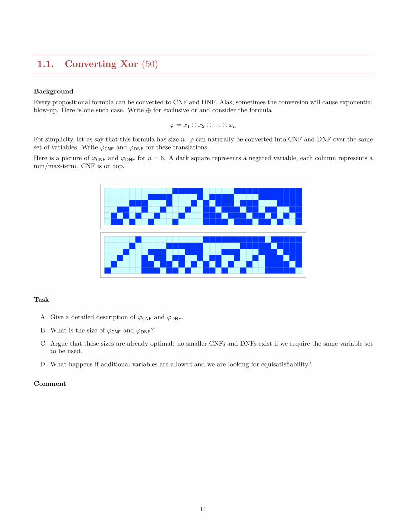
BackgroundEvery propositional formula can be converted to CNF and DNF. Alas, sometimes the conversion will cause exponentialblow-up. Here is one such case. Write ⊕ for exclusive or and consider the formula

ϕ = x1 ⊕ x2 ⊕ . . .⊕ xn

For simplicity, let us say that this formula has size n. ϕ can naturally be converted into CNF and DNF over the sameset of variables. Write ϕCNF and ϕDNF for these translations.Here is a picture of ϕCNF and ϕDNF for n = 6. A dark square represents a negated variable, each column represents amin/max-term. CNF is on top.

Task

A. Give a detailed description of ϕCNF and ϕDNF.

B. What is the size of ϕCNF and ϕDNF?

C. Argue that these sizes are already optimal: no smaller CNFs and DNFs exist if we require the same variable setto be used.

D. What happens if additional variables are allowed and we are looking for equisatisfiability?

Comment

11

1.2. Math Profs (50)

BackgroundHere is a problem in the spirit of Lewis Carroll: a number of mildly absurd assumptions is given and one has to showthat a certain conclusion follows from them. Here are the assumptions:

1. Good-natured tenured mathematics professors are dynamic.

2. Grumpy student advisors play slot machines.

3. Smokers warding Hawaiian shirts are phlegmatic.

4. Comical student advisors are mathematics professors.

5. Untenured faculty who smoke are nervous.

6. Phlegmatic tenured faculty members who wear Hawaiian shirts are comical.

7. Student advisors who are not stock market players are scholars.

8. Relaxed student advisors are creative.

9. Creative scholars who do not play slot machines wear Hawaiian shirts.

10. Nervous smokers play slot machines.

11. Student advisors who play slot machines are nonsmokers.

12. Creative stock market players who are good-natured wear Hawaiian shirts.

Task

A. Formalize these assumptions in propositional logic. Needless to say, you can assume that “phlegmatic” is theopposite of “dynamic” and so on.

B. Conclude from the assumptions that no student advisors are smokers. Make sure that your argument is clearand concise.

CommentDoublecheck that your formalization is correct, otherwise the proof will turn into a big mess.

12

1.3. Hats (50)

BackgroundA prison warden is bored, and decides to amuse himself with a little game. He blindfolds three prisoners A, B andC, and places hats on their heads. He selects the hats from a supply of three white and two red hats. He hides theremaining two hats. He then explains to the prisoners what he has done, and that he is about to remove the blindfoldsfrom A and B, but they are not allowed to peek at their own hats. C will remain blindfolded. After removal of theblindfolds, he tells the prisoners this:

If you can tell me the color of your hat, you will be released from prison. To discourage guessing, a wronganswer will cost you your head. If you prefer, you can ask to be lead back to your cell.

The following happens:

• A says that he is unable to ascertain the color of his hat, and goes back to his cell.

• Then B says that he too is unable to ascertain the color of his hat, and goes back to his cell.

• But now C claims to know the color of his hat. C tells the warden, and gains his freedom.

TaskDetermine the color of C’s hat, and explain his reasoning.

13

1.4. Proof Patterns (50)

BackgroundWrite bxc for the largest integer less than or equal to a real x.

Task

A. Direct

• a, b odd implies a · b odd.• a 6= 0, ab = ac implies b = c.• Show that bx+ yc ≥ bxc+ byc for any two reals x and y.• Show that bbxc/nc = bx/nc for any real x and positive integer n.

B. Contradiction

• n+ 1 passwords are given to n students implies some student has at least two passwords.• There are infinitely many primes.• √p is irrational for all primes p.• The equation x3 + x+ 1 = 0 has no rational solution.

C. Contrapositive

• a2 odd implies a odd.• f2 injective implies f injective.• w primitive implies wop primitive.

D. Case analysis, bootstrapping

• Find all real x such that |x− 1| < |x− 3|.• Show that bbxc/nc = bx/nc for any real x and positive integer n.• Let f be a real function such that f(x + y) = f(x) + f(y). Show that for all rational r and real x:f(xr) = r f(x).

• Show that bxc+ bx+ 1/3c+ bx+ 2/3c = b3xc for any real x.

E. Elegance

• An elimination tournament begins with 342 players. How many games are played until the winner isdetermined?

• Two bicycles are moving towards each other, each with a speed of 10 miles per hour. They are ten milesapart initially, and a dog runs back and forth between them, at a speed of 20 miles per hour. How far hasthe dog gone when the bicycles meet?

14

1.5. Irrationality (50)

BackgroundIrrationality of certain real numbers like

√2 is usually established by tedious divisibility arguments. Here is an example

of a more geometric argument. Define the golden ratio to the ratio of side-lengths (short one first) of a rectangle withthe property that if one removes the square constructed over the shorter side, one obtains a rectangle of the sameproportion.

Task

A. Just as a warmup, show that √p is irrational for all primes p.

B. Show that the golden ratio exists by using a continuity argument. Hint: start with a unit square.

C. Show that the golden ratio is irrational. Hint: consider the “remove square” operation from above.

Comment

15

1.6. Circle Divisions (50)

BackgroundConsider a circle and pick n distinct points on its perimeter. Then draw all possible chords between these points toobtain a subdivision. Assume that no three lines intersect in one point in the interior of this subdivision. Write Cnfor the number of regions.

Task

A. Argue that Cn is well-defined.

B. Calculate the value for Cn for n ≤ 5.

C. The last part suggests a simple closed form for Cn. Which one?

D. Argue that the apparent closed form is quite wrong as follows: consider a disk of radius one meter and , say,n = 30. Think of having 30 pegs connected by very thin thread.

E. Hard: Come up with closed form for Cn.

Comment

16

1.7. Infinitude of Primes (50)

BackgroundAround 300 BCE, Euclid provided the following well-known proof that there are infinitely many primes. Let p1, . . . , pnbe a finite set of primes and set q = p1 · . . . ·pn+1. Then q is not divisible by any of the pi and hence must be divisibleby some prime p different from all the pi. Here are two other ways to show that there are infinitely many primes.The first uses Fermat numbers Fn = 22n + 1, the second uses Mersenne numbers Mn = 2n − 1. Incidentally, it is anopen problem whether infinitely many Fermat/Mersenne numbers are prime. It is known that Fn is not prime for5 ≤ n ≤ 32; the currently largest known Mersenne prime is 243,112,609 − 1.

Task

A. Show that all Fermat numbers are pairwise coprime. Conclude that there are infinitely many primes. Hint:consider the product of the first n Fermat numbers.

B. Let p prime and show that Mp has a prime factor larger than p. Conclude that there are infinitely many primes.

17

1.8. True/False/Random (50)

BackgroundThe following puzzles ask for a way to extract correct information from various oracles. Only yes/no questions can beasked from the oracles. Alas, the oracles have three different modes (moods): T , they speak the truth; F , they alwayslie; and R, they flip a coin (in their heads, of course) and give a random yes/no answer. Sometimes the oracle do notanswer in English but in their own language. They will consistently say “ya” or “da,” but unfortunately no mortalknows which is yes and which is no.The puzzles also involve envelopes, some of which contain $10,000 (pace Romney). An empty envelope cannot bedistinguished from one containing money by visual inspection alone.

Task

A. Three envelopes lie in a row on a table, two of them contain money. You are to point at one of the envelopesand ask a single question. If you point at a loaded envelope the oracle goes into T mode; otherwise it drops intoR mode.

B. There is one envelope on the table. The oracle is in T or F mode. You are to ask a single question.

C. There is one envelope on the table. The oracle is definitely in T , but she is speaking her own language. You areto ask a single question.

D. Now there are three oracles A, B and C but no envelopes. Exactly one of them is T , F and R mode, respectively,in some order. You are to ask three questions in order to determine their modes.

E. Same as last, but now they are not speaking English.

Comment For the last two parts, there is no requirement that each oracle receives a question. And, of course, thesecond question may depend on the answer to the first and so on. There is no probability distribution on R oracleanswers.

18

1.9. Magic Words (50)

Background The great magician Chidur poses the following problem to his apprentice. Being exceedingly powerful,Chidur can associate words with special properties. In this case, he has chosen to associate one of three propertieswith each word: healing, neutral or deadly. The apprentice is fairly new, so Chidur only uses words over the uppercaseLatin alphabet A,B, . . . , Z, words like “ABRACADABRA”. Chidur abhors the empty word.Alas, Chidur refuses to explain directly how he has distributed the properties. All he will tell the hapless apprenticeis this:

• Every word has exactly one property.

• Some pairs of words are exalted. In particular:

– All pairs (XwX,w) are exalted where w is any word.– If (u, v) is exalted then (Y u,Xv) is also exalted.– If (u, v) is exalted then (Zu, vop) is also exalted.– If (u, v) is exalted then (Wu, vv) is also exalted.

• If (u, v) is exalted and u is neutral then v is deadly.

• If (u, v) is exalted and u is deadly then v is neutral.

Task

A. Describe a formal model for this problem and explain how your model correctly represents healing words.

B. Find all shortest healing words.

Comment

19

1.10. Syllogisms (50)

BackgroundArguably the first noteworthy foray into mathematical logic was undertaken by Aristotle in the 4th century BCE. Hestudied patterns of inference involving two premisses and one conclusion. Here is one classical example:

All men are mortal. major premissAll Greeks are men. minor premissAll Greeks are mortal. conclusion

In the example, “men” is the subject term and “mortal” is the predicate term in the major premiss. In modernnotation one could write the major premiss as ∀x (man(x) → mortal(x)). Of course, first-order logic was still morethan two millennia away when Aristotle did his work. Note that the two premisses have to fit together, in the examplethe predicate term in the minor premiss is the same as the subject term in the major. Also, one wishes to considerlogical constructs other than universal quantification. More precisely, we want to admit four forms:

form type classificationA All S is P universal positiveE No S is P universal negativeI Some S is P existential positiveO Some S is not P existential negative

So the example would be characterized as being of type AAA. Also note that this classification is clearly inspired bynatural language, not by first-order logic. Here is a valid AEE type inference:

All rodents have fur.No snake has fur.No snake is a rodent.

The “fitting together” part is regulated like so by introducing four admissible figures:figure 1 figure 2 figure 3 figure 4

major M P P M M P P Mminor S M S M M S M Sconcl. S P S P S P S P

Thus example 1 is figure 1, example 2 is figure 2.By choosing one of the 16 form combinations for the premisses and one of the 16 combinations of form and figure forthe conclusion we get 64 possibly syllogisms. Alas, not all of them are valid.

Task

A. Find two valid syllogisms for each of the four figures.

B. Write a program to determine all valid syllogisms.

C. Explain in detail why your analysis in part (B) is correct.

Comment Be careful with empty domains. You might find it helpful to rewrite the forms in terms of sets or evenfirst-order logic. Note, though, that the syllogism testing program does not require high powered tools.

20

1.11. Boolean Set Operations (50)

Task

A. A ∩B = B ∩A

B. (A−B) ∩ C = (A ∩ C)−B

C. A− (B ∩ C) = (A−B) ∩ (A− C)

D. A ∩ (B ∪ C) = (A ∩B) ∪ (A ∩ C)

E. A− (B ∪ C) = (A−B) ∩ (A− C)

F. A− (B − C) = (A−B)− C

G. (A−B)− C = (A− C)−B

21

1.12. Finsler (50)

BackgroundIn 1926 Paul Finsler published a paper “Formale Beweise und die Entscheidbarkeit” in which he argues that formal-ized systems of mathematics are insufficient. His argument goes like this: consider all unobjectionable proofs thatdemonstrate that the number of 0’s in a specific sequence S ∈ 2ω is finite or infinite. For example, if S has a 0 inposition n iff n is prime then Euclid’s standard argument establishes that there are infinitely many 0s in S. Noworder all these proofs, say, in length-lex order, yielding a sequence (Pn)n≥0 of proofs where Pn deals with sequenceSn. Construct the anti-diagonal sequence S′. Then our formal proof system cannot determine whether the number of0s in S′ is finite or infinite.But in reality S′ has infinitely many 0s. To see why note that there are infinitely many proofs that the constantsequence 1111 . . . has finitely many 0s. Hence S′ must have infinitely many 0s.Note that Godel’s seminal paper appeared 5 years later.

Task

A. Critique Finsler’s argument.

Comment

22

1.13. Sums and Products (50)

BackgroundWhen dealing with communication protocols and security, one often has to use more than just plain propositionallogic: one also has to be able to draw conclusions from the (supposedly intelligent and rational) behavior of otherpeople (or computers). These problems can be quite hard in general, but the one below is manageable: it requiressome logical reasoning, as well as brute force calculation.

TaskSuppose x and y are two integers in the range from 2 to 99. Compute their sum and product, and reveal the sum toMs. S, and the product to Mr. P. Initially, neither S nor P knows the other value.

S : x+ y = s

P : x · y = p

They now start to communicate as follows:

• A day later, S calls P and tells him that he cannot possibly know x and y.

• P thinks about this for a while, calls back S and tells her: “I now know x and y.”

• S ponders for a while, calls up P, and says: “I too know the numbers.”

A. What are the two numbers? Explain how you come to your conclusion.

CommentWe have to make some tacit assumptions here: both S and P are rational beings, they know arithmetic, they don’tlie. Try to be as clear and convincing in your reasoning as possible.

23

1.14. Tautology Testing (50)

BackgroundAs pointed out in class, testing whether a propositional formula is a tautology is trivial in principle (just build thetruth table) but very hard when it comes to efficiency. All known algorithms for the decision problem Tautology arecatastrophically slow on some inputs. A fast, general algorithm would be a major breakthrough in CS – but, thereare good reasons to believe that really fast algorithms do not exist.At any rate, sometimes the test is easy, most notably when the formula is in CNF (conjunctive normal form).

Task

A. Explain exactly why Tautology is easy if the input is in CNF.b) Fred Hacker (who went to MIT) now has the following bright idea. We know that every formula can betransformed into an equivalent one in CNF. So, to crack Tautology for an arbitrary formula, Fred proposes a2-step algorithm:

• First translate the given formula into CNF.• Then use the very fast algorithm from part (A).

Fred really would like to patent this idea. What will he hear from the patent office? Why?

Comment

24

1.15. Normal Forms (50)

Background

TaskConvert each of the following formulae into NNF (negation normal form), CNF (conjunctive normal form), DNF(disjunctive normal form) and INF (implicational normal form). Make sure to simplify whenever possible, so theexpressions remain short. Also, in your solution, show some intermediate steps, not just the final result.

A. ¬((p ∨ q) ∧ (r ∨ s ∨ t)).

B. ¬((p ∧ q) ∨ ¬(r ∧ s ∧ t)).

C. ((p ∨ s) ∨ (q → p)) ∧ (p → (q → s)).

D. ¬(p ∧ q ∧ ((¬(p ∧ r ∧ t)) ∨ s ∨ p)).

Comment

25

1.16. DNF (50)

BackgroundSuppose we have set variables x = x1, . . . , xn, all ranging over the subsets of some fixed ground set 1. We areinterested in equations built from these variables using the operations union, intersection and complement (where thecomplement of x is understood to be 1−x). An expression z1 ∩ z2 ∩ . . .∩ zn where zi is a literal for xi (i.e., zi = xi orzi = 1− xi) is a min-term (over x). An expression is in disjunctive normal form (DNF) if it is a union of min-terms.

Task

A. For legibility, we use a, b and so on as variables. Show that the conditions

a ∩ b ⊆ (c ∩ d) ∪ (c ∩ d), b ∩ c ⊆ (a ∩ d) ∪ (a ∩ d), a ∩ b ⊆ c ∩ d, c ∩ d ⊆ a ∩ b

together imply that

a ∩ b ∩ c = ∅.

Then show that they also imply that

a ∩ b ∩ c = ∅.

B. Show that every equation F = G or sub-equation F ⊆ G can be rewritten in the form H = ∅.

C. Use Shannon expansion to show that every expression has an equivalent DNF.

D. We are given equations Fi(x) = ∅, i = 1, . . . , k and would like to conclude that they imply G(x) = ∅. Show thatthis conclusion is valid iff every min-term in G is also a min-term in one of the Fi.

E. Show how to rewrite given equations Fi(x) = ∅, i = 1, . . . , k into an equivalent single equation F (x) = ∅.

F. Suppose G(xk+1, . . . , xn) uses only the indicated variables. Show that the most general conclusion G that canbe drawn from F (x) is ⋂

z∈2kF (z, xk+1, . . . , xn)

where z = (x1, . . . , xk).

G. Determine the most general conclusion that can be drawn from the sub-equations given in part (A).

Comment

26

1.17. Dual Formulae (20)

BackgroundFor this problem let us only consider Boolean connectives ¬, ∨ and ∧ (no implication, xor etc.) For any propositionalformula ϕ dual ϕop to be obtained from ϕ by interchanging ∧ and ∨, as well as ⊥ and >. For example, (p ∨ ¬q)op =p ∧ ¬q.Similarly, for a truth assignment σ, define [[p]]σop = [[¬p]]σ (i.e., flip the truth values for all propositional variables),and then generalize inductively to all formulae.A formula ϕ is self-dual if ϕ and ϕop are equivalent. For example, p and ¬p are both self-dual but p ∧ q is not.

Task

A. What would the dual of a biconditional ϕ ⇔ ψ be?

B. Show that the dual is an involution: (ϕop)op = ϕ.

C. Show that [[ϕop]]σ = [[¬ϕ]]σop .

D. Show that ϕ is a tautology if, and only if, ϕop is a contradiction.

E. Show that two formulae are equivalent, if, and only if, their duals are equivalent.

F. Find a non-trivial example of a self-dual formula in three variables. Generalize to any odd number of variables.

Comment The first few properties are more or less obvious, but try to come up with clear, elegant proofs. For thelast part think about counting. It may help to think about Boolean functions rather than formulae: f is self-dual ifff(x1, . . . , xn) = ¬f(¬x1, . . . ,¬xn).

27

1.18. Biconditionals (50)

BackgroundSuppose we have propositional variables p1, . . . , pn. Define formulae ϕ1 = p1 and

ϕi+1 = ϕi ↔ pi+1.

For example, ϕ3 = (p1 ↔ p2) ↔ p3.

Task

A. Show that the biconditional is associative and commutative in the sense that the corresponding rearrangementsdo not affect truth values:

ϕ ↔ ψ ≡ ψ ↔ ϕ

(ϕ ↔ ψ) ↔ ρ ≡ ϕ ↔ (ψ ↔ ρ)

B. Give a simple characterization for the truth of ϕn in terms of the truth values of the propositional variables pi.

Comment The simpler your characterization in part (B) the better.

28

1.19. Biconditionals (50)

BackgroundConsider a tiny logical system L, a subsystem of propositional logic with just one operation binary, the biconditional↔, and the constant ⊥. We assume the following axioms where p, q and r are propositional variables.

p↔ p

(p↔ q)↔ (q ↔ p)((p↔ q)↔ r)↔ (p↔ (q ↔ r))

Rules of inference are “modus ponens” (with the biconditional instead of the standard implication) and substitution.Note that negation is expressible in L since ¬p ≡ p↔ ⊥. Likewise we could define > as ¬⊥.Let us say that two formulae ϕ and ψ are L-equivalent if ϕ ` ψ and ψ ` ϕ.

Task

A. Find a reasonable normal form ϕ′ for L-formulae ϕ (meaning that ϕ′ has a particular syntactic structure and isL-equivalent with ϕ).

B. Let ϕ be a formula. Show that the following three assertions are equivalent:

(a) ϕ is a tautology.(b) ϕ is derivable in L.(c) Every propositional variable and ⊥ appears an even number of times in ϕ.

Comment

29

1.20. Symmetric Differences (50)

BackgroundWe write X ∆Y for the symmetric difference of X and Y . Let’s say that X and Y differ evenly if X ∆Y is finite andhas even cardinality. Given a ground set A we say that A obeys principle (P) if there is a function π : P(A) → Asuch that for any two sets X,Y ⊆ A we have: π(X) = π(Y ) iff X and Y differ evenly.

Task

A. Show that “differ evenly” is an equivalence relation.

B. Show that for any finite A, |A| > 1, principle (P) obtains.

C. Show that for any infinite A principle (P) fails.

D. What happens if we replace P(A) with Pω(A), the set of finite subsets of A?

Comment

30

1.21. UnEqual Satisfiability (50)

BackgroundRecall that 3SAT is the decision problem where the instances are propositional formulae in 3CNF and one needs tocheck whether the formula is satisfiable. Here is a variant of this problem. The instances are again formulae in 3CNFand we are looking for a satisfying truth assignment. However, this time we require not just that every clause of theformula contain a literal that evaluates to true but also that it contains a literal that evaluates to false. We writeUESAT for this problem.

Task

A. Show that for every truth assignment σ and every contradiction in 3CNF there is a clause all of whose literalsevaluate to false, and another clause all of whose literals evaluate to true.

B. Show that 3SAT is polynomial time reducible to UESAT.

Comment

31

1.22. Davis-Putnam (50)

BackgroundRecall the Davis-Putnam algorithm to determine satisfiability of a propositional formula S in CNF.

• Remove all unit clauses.

• If there is an empty clause: return False.

• If there are no clauses left: return True.

• Let S′ be the current formula. Pick a literal x in S′. Call the algorithm on S ∪ x and S ∪ x

TaskApply the algorithm to the following formulae. If the formula turns out to be satisfiable, determine a satisfyingassignment.

A. ((a, b, c), (¬a, b, c), (¬a,¬b, c), (¬b,¬c))

B. ((a, b), (a, c), (b, c), (¬a,¬b), (¬a,¬c), (¬b,¬c), (a, b, c))

32

1.23. Quantifiers (50)

Background

Task Which of the following sentences is valid? Give reasons for your answer.

A. ∀x ∃ y φ(x, y) → ∃ y ∀xφ(x, y).

B. ∃ y ∀xφ(x, y) → ∀x∃ y φ(x, y).

C. ∀x∃ y φ(x, y) → ∀ y ∃xφ(x, y).

D. Show that ` ∀xφ(x)↔ ¬∃x¬φ(x).

E. Show that ` ∃xφ(x)↔ ¬∀x¬φ(x)

Comment

33

1.24. Predicate Badgers (50)

BackgroundRecall the Lewis Carroll puzzles from last week.

1. Animals are always mortally offended if I fail to notice them.

2. The only animals that belong to me are in that field.

3. No animal can guess a conundrum, unless it has been properly trained in a Board-School.

4. None of the animals in that field are badgers.

5. When an animal is mortally offended, it always rushes about wildly and howls.

6. I never notice any animal, unless it belongs to me.

7. No animal, that has been properly trained in a Board-School, rushes about wildly and howls.

One can handle this problem nicely in propositional logic, but it can also be expressed quite naturally in predicatelogic. To preserve everyone’s sanity, use the following variables with intended meaning as indicated in the table.• N notice an animal

• M is mine

• F in the field

• B a badger

• O offended

• R rushes about

• S trained at school

• C can guess a conundrumFor example, the first assertion can be written as

∀x (¬N(x) → O(x)).

Task

A. Rewrite all of Carroll’s assertions as formulae in predicate logic. State clearly what the intended meaning of therelation symbols is, and what the intended range of the quantifiers is.

B. Then use natural deduction to show that the conclusions you drew about badgers last week can really be derivedin a formal manner.

Comment You may use conversions between existential and universal quantifiers. Also, feel free to use any equiva-lences that do not involve quantifier manipulations, and focus in your proof on the latter.The argument is a bit long (24 lines in my solution), but all very mechanical. You only need to invoke a few inferencerules.

34

1.25. Verifying Frege (50)

BackgroundFrege’s system uses a number of simple propositional axioms. Needless to say, all these axioms are tautologies. Hereare two of them:

(a → (b → c)) → ((a → b) → (a → c))(a → (b → c)) → (b → (a → c))

Let ϕ be the following formula over variables a, b, . . . , h.

(a ∨ b ∨ c ∨ d ∨ e)∧¬((a ∧ b) ∨ (a ∧ c) ∨ (a ∧ d) ∨ (a ∧ e) ∨ (b ∧ c) ∨ (b ∧ d) ∨ (b ∧ e) ∨ (c ∧ d) ∨ (c ∧ e) ∨ (d ∧ e))∧

((a ∧ b) ∨ (a ∧ c) ∨ (a ∧ h) ∨ (b ∧ c) ∨ (b ∧ h) ∨ (c ∧ h)) ∧ (c ∨ h) ∧ (a ∨ h)

It’s a bit large, but is not random.

Task

A. Convert the Frege formulae into NNF, CNF and DNF.

B. Verify that the Frege formulae are tautologies by using resolution.

C. Find a satisfying truth assignment for ϕ using the Davis/Putnam algorithm.

Comment If you are too lazy to do this by hand you can implement the algorithms. That’s more work, but youwill understand the algorithms much better at the end.

35

1.26. Natural Deduction (50)

BackgroundUse the natural deduction system as introduced in class.

Task

A. Show that all the rules in Natural Deduction involving ∧ and → are sound: whenever the premises are trueunder some truth assignment, so are the conclusions.

B. Give a derivation for p → (q → r), p → q ` p → r.

C. Give a derivation for p ∧ q ` ¬(¬p ∨ ¬q).

D. Give a derivation for p ∨ q ` ¬(¬p ∧ ¬q).

E. Give a derivation for ¬p ∨ q ` p → q.

F. Give a derivation for p → q ` ¬p ∨ q.

Comment

36

1.27. Natural Deduction in Predicate Logic (50)

BackgroundSome of the arguments require side conditions for variables, make sure to spell them out clearly.

Task

A. ` ∀xφ(x)↔ ∀ z φ(z)

B. ` ∀x (φ(x) ∧ ψ(x))→ ∀xφ(x) ∧ ∀xψ(x)

C. ` ∀xφ(x) ∨ ∀xψ(x) → ∀x (φ(x) ∨ ψ(x))

D. φ → ψ ` φ → ∀xψ.

E. φ → ψ ` ∃xφ→ ψ.

Comment

37

1.28. Maximally Consistent Sets (50)

BackgroundRecall that a set of formulae Γ is consistent if not Γ ` ⊥. It is deductively closed if for any formula φ we have Γ ` φimplies φ ∈ Γ. Γ is maximally consistent if no proper superset of formulae is still consistent.

Task Let Γ be a set of formulae that is both consistent and deductively closed. Show that the following are equivalent:

A. Γ is maximally consistent.

B. For any formula φ, φ ∈ Γ or ¬φ ∈ Γ.

C. φ ∨ ψ ∈ Γ implies φ ∈ Γ and ψ ∈ Γ.

Comment

38

1.29. One Unary Function (50)

BackgroundThe expressiveness of first order logic depends somewhat on the underlying language (though even a single binarypredicate is already very powerful: it suffices for set theory). One particularly simple case is where the language onlyhas one unary function symbol f . As always, we allow equality so one can write things like f(f(x)) = y. For anycollection Γ of sentences, the models (if they exist) are just structures A = 〈A,F 〉 where F : A→ A .Let us call two points a, b ∈ A connected if fn(a) = fm(b) for some n,m ≥ 0 (this is a first order statement only whenn and m are fixed). Note that connectedness is an equivalence relation and can be used to decompose our structures.

Task

A. Show how to express the assertion “f is injective but not surjective”.

B. Find the shortest formula to express the assertion “there is a 3-cycle”.

C. Find the shortest formula to express the assertion “there is a 4-cycle”.

D. Describe all connected structures.

E. Describe all models of the axiom ∀x (f10(x) = x).

CommentNote that a 3-cycle must involve 3 distinct points; a fixed point is not a 3-cycle.You might suspect that there is a decidability result somewhere, and there is. However, the proof is quite complicatedand the complexity of the decision algorithm is not even elementary.

39

1.30. Formulae over Q and R (50)

BackgroundConsider the usual structure R of the real numbers, and the structure of the rational numbers, Q. Let 2 be a constantdenoting the number two, more precisely 2 = 1 + 1. For each of the following formulae, determine whether it holdsover either structure.

Task

A. ∀x ∃ y (x = y + y)

B. ∀x∃ y (x > 0 → x = y · y)

C. ∀x, y ∃ z (x > y → x > z ∧ z > y)

D. ∃x, u, v, w (x · x · x = u ∧ x · x = v ∧ 2 · x+ w = 0 ∧ u+ v + w = 2 ∧ x+ 1 6= 0).

Comment

40

1.31. Graphs and FOL (30)

BackgroundFor this problem we consider the FO language with just one binary relation symbol E. We can think of suitablestructures as directed graphs G = 〈V,E〉: x E y means that there is an edge from x to y. When we say that a formulaϕ expresses property such-and-such we mean that G |= ϕ if, and only if, G has the property in question.Some standard graph properties can be expressed in FOL, others can not. In the following, try to make your formulaeas small as ever possible and explain how they work.

Task

A. Express the property “there is a k-cycle” as a FO formula ϕk.

B. Express the property “every vertex lies on a k-cycle” as a FO formula ϕ′k.

C. Express the property “the graph has n vertices and is strongly connected” as a FO formula χk.

D. Show that there is no FO formula that expresses “the graph is strongly connected.”

CommentRecall that a digraph is strongly connected if any two vertices lie on a cycle. For part (A) note that we mean a cycleof length exactly k. For example, a self-loop does not count as a 2-cycle. For part (D) you probably want to usecompactness to construct a bad infinite graph.

41

1.32. Presburger and Skolem Arithmetic (40)

BackgroundPresburger arithmetic is the fragment of arithmetic that has addition but no multiplication; Skolem arithmetic is thefragment that has multiplication but no addition. Both turn out to have decidable first-order theory (in stark contrastto general arithmetic).It is a folklore result that addition is rational and even synchronous. More precisely, there is a synchronous relationα(x, y, z) that expresses x+y = z where the numbers are given in reverse binary. There is no corresponding synchronous(or even rational) relation µ(x, y, z) for multiplication. However, we can choose a different encoding from N+ to 2?that makes multiplication rational. Alas, this encoding is slightly strange and mangles addition badly.

Task

A. Show that the addition predicate α is rational for numbers in reverse binary.

B. Argue that α is actually synchronous.

C. Show that multiplication is not rational for numbers in reverse binary.

D. Concoct an encoding of the positive natural numbers that makes multiplication rational. Hint: think aboutprimes.

E. Exlain why your encoding does not work for addition.

Comment For part (A) you can either write a rational expression or draw a diagram. This is a bit of a pain;whatever you do, try to make it look nice.For part (C) you may freely use pumping lemmings and the like.For part (E) no formal proof is necessary, just a reasonable explanation.

42

1.33. Weak Arithmetic (50)

BackgroundConsider a first-order language with symbols: constant 0, unary function ′ and binary functions + and ∗. The followingaxiom system Q formalizes elementary arithmetic, much like the well-known system due to Peano does. However, Qis much weaker than Peano arithmetic as you will show in a moment. It is a surprising and hard to prove feature ofQ, though, that every computable function can be represented in Q. Don’t try.Here are the axioms for Q:

1. x′ = y′ → x = y

2. x′ 6= 0

3. x 6= 0 → ∃ y (y′ = x)

4. x+ 0 = x

5. x+ y′ = (x+ y)′

6. x ∗ 0 = 0

7. x ∗ y′ = (x ∗ y) + x

Note that these axioms are trivially satisfied in the standard model N.

TaskShow that all the following assertions are not provable in Q.

A. ′ has no fixed points

B. + is associative

C. + is commutative

D. ∗ is associative

E. ∗ is commutative

Comment

43

1.34. Pierce Arithmetic (50)

BackgroundDuring a lecture in 1879, C. S. Pierce suggested a formal system of arithmetic. His original description is in ordinaryEnglish and reads like so:

1. Every number by process of increase by 1 produces a number.

2. The number 1 is not so produced.

3. Every other number is so produced.

4. The producing and produced numbers are different.

5. In whatever transitive relation every number so produced stands to that which produces it, in that relation everynumber other than 1 stands to 1.

6. What is so produced from any individual number is an individual number.

7. What so produces any individual number is and individual number.

The system is similar in spirit to efforts by Dedekind and Peano, but slightly different in detail.

TaskWrite x ∈ N to indicate that x is a number, and in particular ∀x ∈ N and ∃x ∈ N for quantification over numbers.P (x, y) means “x by process of increase by 1 produces y” and trns(R) indicates that a binary relation R is transitive.Feel free to quantify over binary relations.

A. Formalize Pierce’s description.

B. Find a potential weakness in this attempt to formalize basic arithmetic. Use your formalization to make yourpoints (unfortunately, the sources are weak, no one knows for sure what Pierce intended).

Comment

44

1.35. Peano Arithmetic (50)

BackgroundPeano arithmetic (PA) is an axiom system for arithmetic on the natural numbers expressed in first order logic, seepage 39pp inhttp://www.andrew.cmu.edu/course/15-354/postscript/FOL-Theories.pdf.This axiom system is powerful enough to prove assertions about computable functions. In fact, functions that are ofpractical use are fully covered by (PA).One important (though slightly boring) task is to show that some definition really yields a total function: the definitionmust cover all possible inputs and must pin down the output uniquely. This is tricky in particular when the functionis defined in terms of equations.

Task

A. Show that (PA) proves commutativity of addition and multiplication.

B. Show that (PA) proves that every primitive recursive function is total.

C. Show that (PA) proves that the Ackerman function is total.

CommentNote that we did not introduce a formal method of proof for first order logic (look at the linked document if you reallywant to know; you will recoil in horror). Still, it is intuitively clear how one can use these axioms in an argument.(PA) is not all powerful, though: there are total computable functions whose totality cannot be established in thissystem. These functions are quite complicated, though.

45

1.36. Interpolation (50)

BackgroundConsider a tautology A → B in propositional logic, say, p∧q → p∨r. This implication can be pulled apart: p∧q → pand q → p ∨ r. Note that the middle formula contains only variables common to both initial formulae.In general, call a formula C an interpolant for A and B if A → C and C → B are tautologies and Var[C] ⊆ Var[A] ∩Var[B]. Write X = Var[A] ∩ Var[B].

Task

A. Consider partial truth assignments α : X → 2 and their possible extensions to full truth assignments. Classifyall possible cases.

B. Use part (A) to explain how to construct an interpolant.

C. Derive an upper bound for the size of the interpolant.

Comment A similar result also holds for first-order logic. The size of the smallest propositional interpolant hasimportant complexity theoretic consequences for problems in NP ∩ co-NP.

46

1.37. Unary and Binary (50)

BackgroundThe following two structures formalize the idea of natural numbers being represented in unary and binary:

Nu = 〈N, S, P, 0, 1〉Nb = 〈N, par, div, em, om, 0, 1〉

Here S stands for successor, P for predecessor; par for parity (so par(x) = x mod 2), div is integer division by 2, andem(x) = 2x, om(x) = 2x+ 1.A (partial) function is recursive over one of these structures if it can be defined from the given primitive operationsusing composition, if-then-else and recursion. We will not give a formal definition (which turns out to be very tedious);instead, here is an example: addition in Nu.

add(x, y) = if y = 0 then x else S(add(x, P (y))).

Note that there are no restrictions against definitions such as f(x) = if x = 0 then 0 else f(S(x)), functions defineby recursion may well be partial.

Task

A. Show how to define S and P by recursion over Nb.

B. Show how to define par, div, em and om by recursion over Nb.

C. Conclude that exactly the same functions are definable by recursion over Nu and Nb.

D. Show that in either case we obtain exactly all computable functions.

Comment

47

1.38. Maps and Powersets (50)

BackgroundBy non-injectivity (Ninj) we mean the assertion that no map of the form f : P(A) → A is injective. Similarly,non-surjectivity (Nsur) means that no map of the form g : A→ P(A) is surjective.Cantor gave a simple proof of (Nsur): given g we can form the set B = a ∈ A | a /∈ g(a) . But B is not in the rangeof g. It follows that the cardinality of P(X) is strictly larger than the cardinality of X.

TaskFor the following arguments avoid indirect proofs, always come up with as direct a line of reasoning as possible. Youmay use other standard assumptions from set theory as needed.

A. Show that (Nsur) implies (Ninj).

B. Show that (Ninj) implies (Nsur).

C. Give a direct proof of (Ninj).

Comment For part (C), take inspiration form Cantor’s argument.

48

1.39. Dedekind Infinity (50)

BackgroundA set A is Dedekind infinite if there is a proper subset B of A and a bijection f : A←→ B . Likewise, a set is Dedekindfinite if no such bijection exists. For example, the natural numbers are Dedekind infinite: consider the map x 7→ x+ 1from N to N+.By contrast, a set A is infinite in the ordinary sense if there is no bijection f : n←→ A where n is a finite Neumannordinal (obtained from ∅ by finitely many applications of S = λx.x ∪ x; no, this is not circular, one can get aroundmentioning “finite” in this definition).

Task

A. Show that a Dedekind infinite set is also infinite.

B. Show that all Dedekind finite sets are finite.

Comment Use whatever machinery from set theory might come in handy.

49

1.40. Functions as Relations (50)

BackgroundLet f : A→ B be a function and ρ ⊆ A×B its graph.

Task

A. Assume ρ is reflexive. What can you say about f?

B. Assume ρ is symmetric. What can you say about f?

C. Assume ρ is transitive. What can you say about f?

D.

Comment

50

1.41. Transitivity and Ordinals (50)

BackgroundA set A is transitive if C ∈ B ∈ A implies C ∈ A. Equivalently,

⋃A ⊆ A. Cheap examples: ∅ is transitive as is ∅;

for more interesting transitive sets see below.The transitive closure of A is the least set B (in the subset order) such that A ⊆ B and B is transitive. We writetc(A) for the transitive closure of A.An ordinal is a transitive set all of whose elements are also transitive.

Task

A. Show that B ⊆ A implies tc(B) ⊆ tc(A).

B. Show that tc(A) = A ∪⋃x∈A tc(x).

C. Show that the operation S(A) = A ∪ A preserves transitivity. Moreover, if A is an ordinal then so is S(A).

D. Show that if all Ai, i ∈ I, are transitive [ordinals] then so is⋃Ai and

⋂Ai.

E. Produce some examples of ordinals, the more the merrier.

CommentOne can show that for any two ordinals A 6= B we have A ∈ B or B ∈ A; they properly extend the natural numbers(interpreted as von Neumann ordinals) and make it possible to measure well-orders.

51

1.42. Universal Relations (50)

BackgroundA binary relation ρ on a set A is universal if ρ = A×A.Below consider two symmetric and transitive relations π and ρ on A.

Task

A. Show that π ∪ ρ universal implies that at least one of π and ρ is already universal.

B. Does the previous claim still hold if ρ is only transitive?

Comment

52

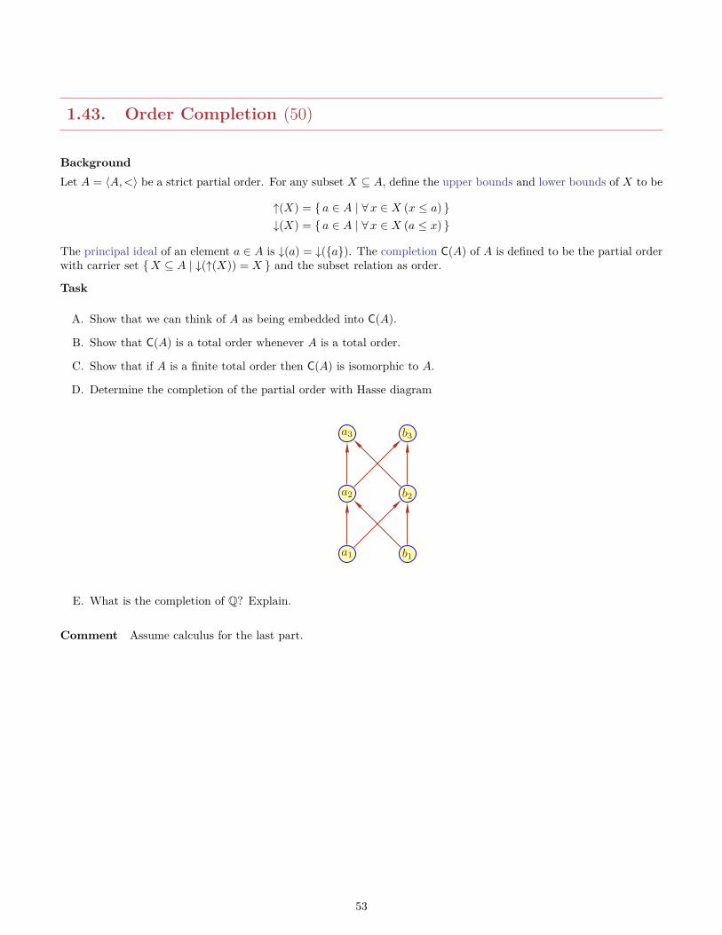
1.43. Order Completion (50)

BackgroundLet A = 〈A,<〉 be a strict partial order. For any subset X ⊆ A, define the upper bounds and lower bounds of X to be

↑(X) = a ∈ A | ∀x ∈ X (x ≤ a) ↓(X) = a ∈ A | ∀x ∈ X (a ≤ x)

The principal ideal of an element a ∈ A is ↓(a) = ↓(a). The completion C(A) of A is defined to be the partial orderwith carrier set X ⊆ A | ↓(↑(X)) = X and the subset relation as order.

Task

A. Show that we can think of A as being embedded into C(A).

B. Show that C(A) is a total order whenever A is a total order.

C. Show that if A is a finite total order then C(A) is isomorphic to A.

D. Determine the completion of the partial order with Hasse diagram

a1

a2

a3

b1

b2

b3

E. What is the completion of Q? Explain.

Comment Assume calculus for the last part.

53

1.44. Pairs (50)

BackgroundSets are by their very definition unordered: a, b = b, a. It is therefore not clear a priori that relations of aritylarger than 1 can be represented as sets. Indeed, the first definitions of ordered pairs as sets emerged in the 1910’s,several decades after the initial development of set theory.As we will see, in set theory one can define pairing functions π and corresponding unpairing functions πi, i = 1, 2,such that

πi(π(x1, x2)) = xi i = 1, 2

for all xi. What is now the standard pairing function is due to Kuratowski and has the form π(a, b) = a, a, b.Here are some others. For legibility, write 0 = ∅ and 1 = ∅.

TaskShow that each of the following functions is a pairing function and determine the unpairing functions.

A. π(a, b) = a,0, b

B. π(a, b) = a,0, b,1

C. π(a, b) = a, a, b

D. π(a, b) = π(0, x) | x ∈ a ∪ π(1, y) | x ∈ b

Comment

54

1.45. Antisymmetry (10)

BackgroundRecall that a binary relation on a set A is antisymmetric if

∀ a, b ∈ A (a ρ b ∧ b ρ a =⇒ a = b)

A weak order is a classical example of an antisymmetric relation.

TaskLet ρ and σ be two antisymmetric relations on some set A. For each of the following relations, determine whetherthey are also antisymmetric. In each case, give a proof or a concise counterexample.

A. complement ρc

B. converse ρop

C. intersection ρ ∩ σ

D. union ρ ∪ σ

E. difference ρ− σ

F. symmetric diff. ρ⊕ σ

G. composition ρ • σ

Comment

55

1.46. Transitivity (10)

BackgroundRecall that a binary relation on a set A is transitive if

∀ a, b, c ∈ A (a ρ b ∧ b ρ c =⇒ a ρ c)

Classical examples of transitive relations are orders and equivalence relations.

TaskLet ρ and σ be two transitive relations on some set A. For each of the following relations, determine whether they arealso transitive. In each case, give a proof or a concise counterexample.

A. complement ρc

B. converse ρop

C. intersection ρ ∩ σ

D. union ρ ∪ σ

E. difference ρ− σ

F. symmetric diff. ρ⊕ σ

G. composition ρ • σ

Comment

56

Chapter 2

Computation

57

2.1. Some Graph Problems (40)

BackgroundIn the following we consider only undirected graphs G = 〈V,E〉. Recall that a vertex cover in G is a subset C ⊆ V suchthat every edge in G is incident upon a vertex in C. A clique in G is a subset C ⊆ V that forms a complete subgraph;an independent set in G is a subset I ⊆ V so that there are no edges between the vertices of I. A Hamiltonian cycleis a simple cycle in G that uses all vertices. These concepts naturally give rise to associated decision problems.

Problem: VertexCover [IndependentSet, Clique]Instance: A graph G = 〈V,E〉, a natural number k, 1 ≤ k ≤ |V |.Question: Does G have a vertex cover [independent set, clique] of size k ?

Problem: HamiltonianInstance: A graph G = 〈V,E〉.Question: Does G have a Hamiltonian cycle?

Task

A. Briefly explain why all these problems are in NP.

B. Show that VertexCover, IndependentSet and Clique are polynomial time equivalent: a polynomial time algorithmfor any one them would translate into a polynomial time algorithm for any other.

C. Show that Hamiltonian can be polynomial time reduced to SAT: given a graph G, one can construct in polynomialtime a Boolean formula ΦG so that G is Hamiltonian iff ΦG is satisfiable.

Comment Note the direction in part (C), this is not a hardness argument.

58

2.2. Fixed Point to Recursion Theorem (30)

BackgroundWe have seen three versions of Kleene’s recursion theorem, the second and fixed point version being:

e?(x) ' F (e?,x)e?(x) ' f(e?)(x)

Task

A. Use the recursion theorem to show that Prec[h, g] is computable whenever h and g are computable.

B. Show that the fixed point version implies the second recursion theorem.

59

2.3. Historical Ackermann (30)

BackgroundThere is a famous example of a computable function defined by recursion that fails to be primitive recursive, theso-called Ackermann function. What is nowadays called Ackermann function is actually a variation (due to RozsaPeter) of the original function B : N3 → N :

B(0, 0, z) = z

B(0, y+, z) = B(0, y, z)+

B(1, 0, z) = 0B(x, 0, z) = 1

B(x+, y+, z) = B(x,B(x+, y, z), z)

Here u+ is shorthand for u + 1. This definition is to be interpreted like a switch statement: always use the firstapplicable rule (so there is no contradiction between, say, equation 3 and 4). It is useful to think of the ternaryfunction B as a family of binary functions Bx:

Bx(y, z) := B(x, y, z).

Task

1. Explain the first three levels B0, B1 and B2.

2. Show that each of the functions Bx is primitive recursive.

3. Compute B3(3, 3).

4. What is the problem in computing B4(4, 4)? How about logB4(4, 4)?

CommentThe first three levels are all well-known and you should recognize the fourth level.

60

2.4. Lists via Coding (30)

BackgroundWe have seen how to define a coding function, an injective map

〈.〉 : N? → N

with “inverse” functions len : N→ N and dec : N× N→ N such that

len(〈a0, a1, . . . , an−1〉) = n,

dec(〈a0, a1, . . . , an−1〉, i ) = ai, i < n

len and dec are primitive recursive and 〈.〉 is primitive recursive for a fixed number of arguments.Our claims is that coding allows us to express discrete, finite structures as natural numbers, and the correspondingoperations as arithmetic functions. In most cases, the functions will turn out to be primitive recursive. We will verifythis claim for lists of natural numbers.Assume the coding function from class so that

〈nil〉 = 0〈a0, . . . , an−1〉 = π(a0, 〈a1, . . . , an−1〉)

Recall that with this setup all of N is the code of some list.

Task

1. Show that the append operation app is primitive recursive:

app(〈a0, . . . , an−1〉, x) = 〈a0, . . . , an−1, x〉

2. Show that the reversal operation rev is primitive recursive:

rev(〈a0, . . . , an−1〉) = 〈an−1, . . . , a0〉

3. Show that the join operation join is primitive recursive:

join(〈a0, . . . , an−1〉, 〈b0, . . . , bm−1〉) = 〈a0, . . . , an−1, b0, . . . , bm−1〉

61

2.5. Node Deletion (20)

BackgroundRecall the node deletion problem mentioned in class.

Problem: Node DeletionInstance: Two graphs G and H, a number k.Question: Can one delete at most k vertices from G to obtain a graph that does not contain H as a subgraph?

Node Deletion appears to be outside of NP: we can guess the nodes to be deleted, but the verification that theremaining graph G′ does not contain H does not seem to be manageable in polynomial time (H is part of the input,not fixed).As always, we use “Node Deletion” as a shorthand for the formal language L ⊆ 2? that describes the yes-instances.

Task

A. Write Node Deletion as a Σ2 Boolean formula.

B. Show that Node Deletion is in NPNP by explaining how the corresponding oracle Turing machine works.

C. Explain how an alternating Turing machine would solve Node Deletion in polynomial time.

62

2.6. Sat Oracle (20)

BackgroundWe have seen that a Sat oracle is helpful when one tries to find a short DNF of a formula. Here is another applicationof such an oracle.

Problem: Least Sat (LSAT)Instance: A Boolean formula ϕ(x1, x2, . . . , xm).Solution: “No” if ϕ is not satisfiable, the lexicographically least satisfying assignment otherwise.

Note that this is a function problem, not a decision problem (though, as always, it could be artificially turned intoone).

Task

A. Prove that there is a polynomial time machine with oracle Sat that solves LSAT.

B. Come up with a decision version of LSAT, and some sort of hardness result.

CommentA precise answer for part (B) is tricky, don’t worry about nailing this perfectly.

63

2.7. Arithmetizing Branching Programs (30)

BackgroundWe saw that arithmetization is a critically important tool when dealing with IP. Unsurprisingly, it’s also useful inother places.Fix a set V = x1, . . . , xm of Boolean variables. Define a branching program over V to be a directed acyclic graph Bwith exactly one node of indegree 0 (input node), two nodes of outdegree 0 (terminals, labeled 0 and 1, respectively)and all non-terminal nodes of outdegree 2 (edges labeled 0 and 1). The non-terminal nodes are labeled by V . B isread-once (ROBP) if all paths from the input node to a terminal encounters each variable in V at most once.So this is essentially a Boolean decision diagram, similar to a ROBDD, but without the important constraints thatmake a ROBDD unique: the same Boolean function may have several ROBPs.We can use arithmetization with ROBP: we assign a polynomial to each node in a ROBP.

• The input node is labeled 1.

• If a node with variable label x is labeled p, then the two out-edges are labeled xp and (1− x)p, respectively.

• A node gets the sum of the polynomials on its in-edges.

The polynomial PB of B is the one labeling the terminal node 1.

Task

A. Construct a ROBP B for the function x1 = x2 ∧ x3 = x4 and compute its polynomial PB .

B. Show that there is a ROBP for the majority function that has size O(m2) (assume m odd for simplicity).

C. Show that PB is a Boolean polynomial that represents the Boolean function defined by B.

D. Find a fast algorithm to test whether a given polynomial p ∈ Z[x] is Boolean.

E. Let Pϕ the Boolean polynomial associated to Boolean formula ϕ. Clearly, Pϕ+1 is Boolean iff ϕ is not satisfiable.What gives?

Comment To preserve TA sanity, write x rather than 1− x in these polynomials.

64

2.8. Branching Programs and BPP (30)

BackgroundSince ROBPs are not unique, we can ask:

Problem: Read-Once Branching Program Equivalence (ROBPEQ)Instance: Two ROBPs B1 and B2.Question: Do B1 and B2 define the same Boolean function?

A priori, it is not clear how randomness helps here: picking some input a ∈ 2m at random and comparing B1(a) andB2(a) may produce the same value with high probability, even though the Boolean functions are different.Recall the Boolean polynomial PB of B from the last question. We will use arithmetic over a finite field for thesepolynomials. It is safe to use Zρ for a sufficiently large prime ρ. We won’t worry about how the right ρ can be found.Here is a little fact about roots of multivariate polynomials over Zρ.Claim: If we pick arguments a ∈ Znρ for a non-vanishing m-variable polynomial P (x) ∈ Zρ[x] uniformly at random,then Pr[P (a) = 0] ≤ md/ρ, where d is the maximum degree of each individual variable.The probabilistic algorithm A looks like this:

• Pick a = a1, . . . , am uniformly at random in Zρ compute the values vi = PBi(a), i = 1, 2.

• Accept if v1 = v2, reject otherwise.

Task

A. Prove the claim about multivariate polynomials by induction on m. You may assume that the case m = 1 iswell-known.

B. Show that algorithm A establishes membership in BPP.

65

2.9. Paths and Trees (30)

BackgroundWe showed that Hamiltonian Cycle is NP-complete. A very closely related problem is

Problem: Hamiltonian PathInstance: A ugraph G = 〈V,E〉.Question: Does G have a Hamiltonian path?

Recall that a spanning tree of a ugraph G = 〈V,E〉 is a subgraph T = 〈V,E0〉 such that T is a tree (connected,acyclic). Consider the following instances: the graph G together with either a bound k, 1 ≤ k ≤ n = |V | (for 1, 2, 3),or a vertex set L ⊆ V (for 4, 5). The questions are as follows: Is there a spanning tree T of G such that

1. T has k leaves.

2. T has at most k leaves.

3. The nodes of T have degree at most k.

4. The set of leaves of T is L.

5. There are no leaves of T outside L.

Task

A. Show that Hamiltonian Path is NP-complete.

B. Show that the five spanning tree problems from above are NP-complete.

Extra Credit: Show that the last problem is hard for any fixed k ≥ 2.

66

2.10. Easy SAT Versions (30)

BackgroundHere are two more “easy” variants of Sat. The first, HornSAT, is obtained by syntactic restriction: the formula hasto be in CNF, and each clause contains at most one unnegated variable (possibly none). Examples:

ϕ = x, y, z, y, z, x

or equivalently, in implicational notation (which is better in this case)

ϕ = x ∧ y ⇒ z, y ∧ z ⇒ ⊥, x

The second variant, XorSAT, is also based on a kind of CNF, but this time the clauses are required to be xors ofliterals. So you can write things such as

(x⊕ y ⊕ z) ∧ (x⊕ z)

You might wish to recall at this point that xor is associative and commutative, and closely related to modulararithmetic: we can think of x ⊕ y as x + y mod 2 with the usual identifications of truth values and arithmetic. SoXorSAT is really just arithmetic modulo 2, in feeble disguise.

Task

A. Show that HornSAT can be solved in polynomial time.

B. Show that XorSAT can be solved in polynomial time.

67

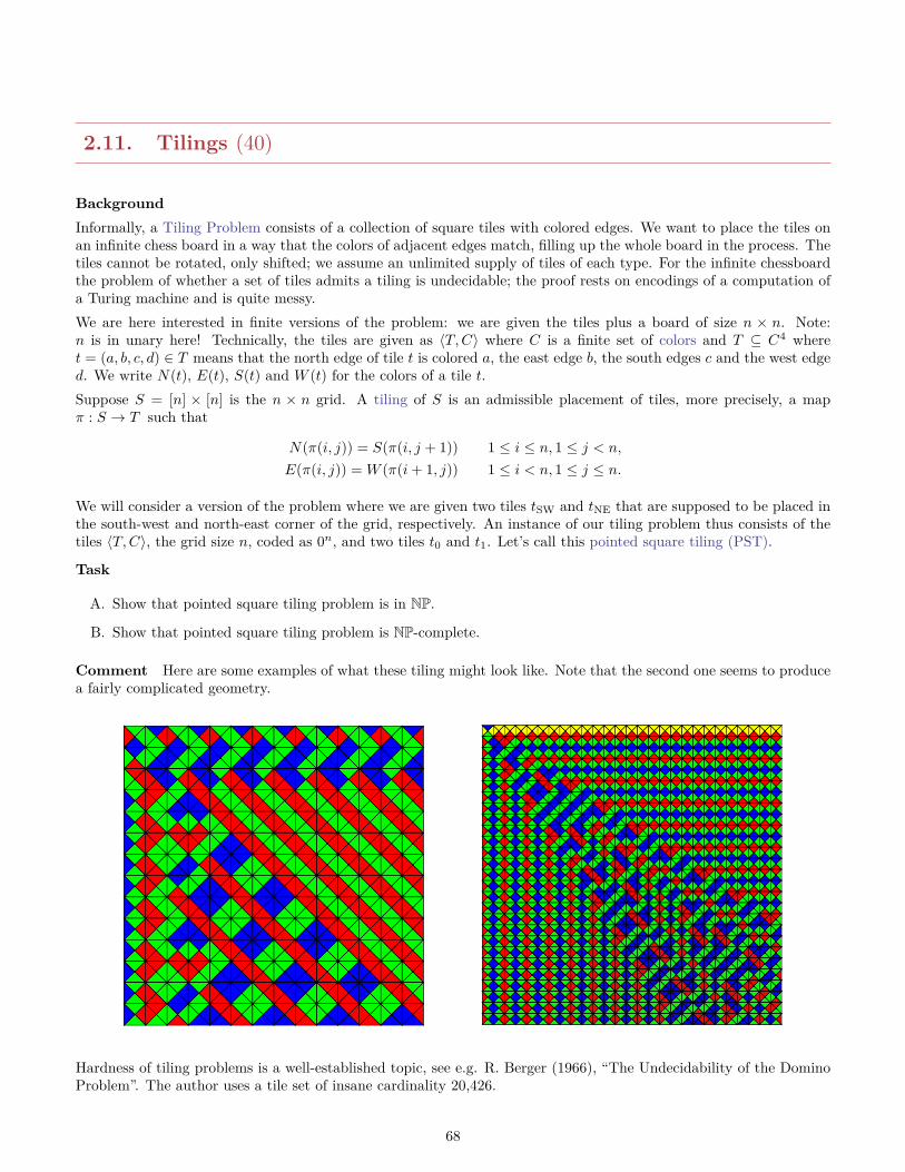
2.11. Tilings (40)

BackgroundInformally, a Tiling Problem consists of a collection of square tiles with colored edges. We want to place the tiles onan infinite chess board in a way that the colors of adjacent edges match, filling up the whole board in the process. Thetiles cannot be rotated, only shifted; we assume an unlimited supply of tiles of each type. For the infinite chessboardthe problem of whether a set of tiles admits a tiling is undecidable; the proof rests on encodings of a computation ofa Turing machine and is quite messy.We are here interested in finite versions of the problem: we are given the tiles plus a board of size n × n. Note:n is in unary here! Technically, the tiles are given as 〈T,C〉 where C is a finite set of colors and T ⊆ C4 wheret = (a, b, c, d) ∈ T means that the north edge of tile t is colored a, the east edge b, the south edges c and the west edged. We write N(t), E(t), S(t) and W (t) for the colors of a tile t.Suppose S = [n] × [n] is the n × n grid. A tiling of S is an admissible placement of tiles, more precisely, a mapπ : S → T such that

N(π(i, j)) = S(π(i, j + 1)) 1 ≤ i ≤ n, 1 ≤ j < n,

E(π(i, j)) = W (π(i+ 1, j)) 1 ≤ i < n, 1 ≤ j ≤ n.

We will consider a version of the problem where we are given two tiles tSW and tNE that are supposed to be placed inthe south-west and north-east corner of the grid, respectively. An instance of our tiling problem thus consists of thetiles 〈T,C〉, the grid size n, coded as 0n, and two tiles t0 and t1. Let’s call this pointed square tiling (PST).

Task

A. Show that pointed square tiling problem is in NP.

B. Show that pointed square tiling problem is NP-complete.

Comment Here are some examples of what these tiling might look like. Note that the second one seems to producea fairly complicated geometry.

Hardness of tiling problems is a well-established topic, see e.g. R. Berger (1966), “The Undecidability of the DominoProblem”. The author uses a tile set of insane cardinality 20,426.

68

2.12. More Tilings (20)

BackgroundRecall the tiling problem from the previous homework: we discussed the pointed square tiling (PST) problem: cana n × n square can be tiled by a given set of tiles (with SW and NE corners fixed)? This problem turns out to beNP-complete.Define the pointed rectangular tiling (PRT) problem as follows: given a “width” n, is there a “height” m so that then×m rectangle can be tiled (again assuming a given SW and NE tile). So the input is the tile set, the 2 corner tiles,and 0n; by contrast, m is not part of the input.

Task

A. Show that pointed rectangle tiling problem is in PSPACE.

B. Show that pointed rectangle tiling problem is PSPACE-complete.

CommentThere is no need to repeat the old PST construction, just explain what is different in this version of the problem.

69

2.13. Simulating Space (20)

BackgroundAs always, assume that f : N→ N is a civilized function.

Task

A. Prove that NSPACE(f) ⊆ TIME(2O(f)) by explaining how to simulate the “space”-machine by a “time”-machine.

B. Where in your proof do you use the assumption that f is not pathological?

CommentYou might want to think about the deterministic case first.

70

2.14. Medians (20)

BackgroundSuppose a = a1, a2, . . . , an is a list of distinct natural numbers, n odd. For simplicity, assume all the numbers arek-bit. Obviously, the median med(a) is uniquely determined.

Task

A. Find an algorithm that computes the median in logarithmic space.

B. Explain in more detail how your algorithm would be executed on a Turing machine.

Comment For the Turing machine, assume the input is given as #a1#a2 . . .#an#. Use as many work tapes as youlike, and write the result to the output tape.

71

2.15. Regular Expression Equivalence (40)

BackgroundTwo regular expressions α and β are equivalent if they denote the same language: L(α) = L(β). Some equivalencesare trivial, say, α1 +α2 is equivalent to α2 +α1, but in general the algebra of regular expressions is fairly complicated(thanks to the Kleene star operation), and it is difficult to check equivalence with algebraic methods. One would liketo understand the complexity of the following decision problem:

Problem: Regular Expression Equivalence (REE)Instance: Two regular expressions α and β.Question: Are α and β equivalent?

Task

A. Describe an algorithm to solve REE.

B. Explain how to implement your algorithm in PSPACE.

CommentREE turns out to be PSPACE-complete (NP-complete for a single-letter alphabet), but we won’t go there.

72

2.16. Immerman-Szelepsenyi (20)

BackgroundThe Immerman-Szelepsenyi theorem in its general form says

For any reasonable function s(n) ≥ logn we have NSPACE(s(n)) = co−NSPACE(s(n)).

Task

A. Explain how this result follows from the nondeterministic path-counting approach discussed in class.

Comment

73

2.17. Graphs and NL (20)

BackgroundRecall that a digraph is strongly connected (SC) if there is a path between any two vertices. There are well-knownpolynomial time algorithms to check whether a graph is strongly connected. Look up Tarjan’s algorithm if you are notfamiliar with it; it’s linear time and space, and absolutely amazing. Since connectivity has to do with path existence,one might wonder how SC relates to NL.Suppose H is an undirected graph. Recall that H is bipartite if we can partition the vertex set into V = V1 ∪ V2 suchthat all edges connect V1 with V2 (so V1 and V2 are both independent sets).

Task

A. Show that SC is in NL.

B. Show that SC is in NL-hard (wrto log-space reductions).

C. Characterize bipartite graphs in terms of their cycles.

D. Show that bipartiteness can be checked in NL.

74

2.18. Small Space (20)

BackgroundWrite bin(x) ∈ 2? for the binary expansion of x ∈ N. Let’s say, LSD first (though the claim also holds for MSD first).Define the languages

K = 0n1n | n ≥ 0 ⊆ 2?

L = bin(0)#bin(1)# . . .#bin(n) | n ≥ 0 ⊆ 0, 1,#?

Recall that SPACE(o(log logn)) is already SPACE(1), but that is as far as one can go.

Task

A. Show that the context-free language K is in L.

B. Show that L is not regular.

C. Show that L is in SPACE(log logn).

75

2.19. Computing Log-Space Functions (40)

BackgroundGiven a transducer M with a separate output tape, it is reasonable to insist that there are no over-writes: everytime the machine writes an output symbol, it moves the head one to the right (and never to the left). If M is alsoSPACE(logn) we call the corresponding function prompt.A more tedious approach to computing a function is to associate it with decision problems describing its ouput, andthen insist that the corresponding languages be “easy.” More precisely, consider bin(z, i) to be ith digit in bin(z) andwrite |z| for the length of bin(z). For a function f define

BIN = x#i | bin(f(x), i) = 1

LEN = x#i | i < |f(x)|

If f is polynomially bounded (in the sense that |f(x)| ≤ |x|O(1)), and both BIN and LEN are in L we call f logish.

Task

A. Show that every prompt function is logish.

B. Show that every logish function is prompt.

76

2.20. SAT Versions (30)

BackgroundSat is usually combined with a constraint to the syntactic form of the input formula. Particularly popular is CnfSatwhere the input is required to bin in CNF, and k−SAT where, in addition, all clauses are required to be of lengthexactly k. In MonoSAT, all the variables in one clause are either positive, or they are all negative.Assume that all formulae are written in terms of the standard de Morgan base ∧,∨,¬.

Task

A. Give a polynomial time algorithm for 2−Sat.

B. Give a fast many-one reduction from CnfSat to 3−Sat.

C. What is the running time of your reduction? (is it poly time?, is it log space?)

D. Give a fast many-one reduction from 3−Sat to MonoSAT.

E. What is the running time of your reduction?

Comment For part (A) and a clause x, y, consider x → y and y → x.

77

2.21. Subset Sum (30)

BackgroundSubset Sum is a standard combinatorial problem:

Problem: Subset SumInstance: A list of natural numbers a1, . . . , an, b.Question: Is there a subset I ⊆ [n] such that

∑i∈I ai = b?

The numbers are all written in binary, you may safely assume that they are all k-bit. So the size of the input isk(n+ 1). To preserve TA sanity, let’s assume they are all written in reverse binary, LSD first.

Task

A. Give a polynomial time reduction from Subset Sum to Sat.

B. Suppose we know in addition that ai ≤ 42 for all i. Find a fast algorithm for Subset Sum and explain its runningtime.

CommentFor (A), first figure out the cases n = 1 and n = 2. You might also want to take a look at problem 3.D.

78

2.22. BDDs (40)

BackgroundBy BDD we always mean ROBDD, using the standard variable ordering

x1 < x2 < . . . < xn < 0, 1

Assume the most basic standard implementation (two terminal nodes, no negation tricks, . . . ) We refer to the numberof nodes in the BDD as its size.

Task

A. What is the size of the BDD for x1 ∧ x2 ∧ . . . ∧ xn.

B. What is the size of the BDD for x1 ⊕ x2 ⊕ . . .⊕ xn.

C. Assume n is even. What is the size of the BDD for

(x1 ⇔ x2) ∧ (x3 ⇔ x4) ∧ . . . ∧ (xn−1 ⇔ xn).

D. What is the size of the BDD that computes addition on two k-bit numbers? For simplicity, assume the ouput isalso k-bit, we simply truncate if there is overflow. Here n = 3k and the bits are grouped as follows:

x1x4 . . . x3k−2 = u

x2x5 . . . x3k−1 = v

x3x6 . . . x3k = w

We want u+ v = w, ignoring overflow.

CommentFor all of these, start with small values of n, and try to figure out what happens when n increases. If you cannot getan exact count, at least indicate the order of magnitude.

79

2.23. Linear Time Reductions (25)

BackgroundA is linear time reducible to B if there is a linear time computable function f : Σ? → Σ? such that xinA ⇐⇒ f(x) ∈B. One can show that this is a pre-order, so we can consider the corresponding equivalence relation ≡lin, producingthe linear time degrees.Notation: A ≤lin B and A ≡lin B.Recall the standard decision problems from graph theory:

Problem: Vertex Cover (VC)Instance: A ugraph G, a bound k.Question: Does G have a vertex cover of cardinality k?

Problem: Independent Set (IS)Instance: A ugraph G, a bound k.Question: Does G have an independent set of cardinality k?

Problem: Clique (CL)Instance: A ugraph G, a bound k.Question: Does G have a clique of cardinality k?

Assume that the graph is given as an n× n Boolean matrix, k is written in binary.

Task

A. Show that linear time reducibility is a pre-order.

B. Show that A ≤lin B, B ∈ TIME(nk) implies A ∈ TIME(nk).

C. Show that VC ≡lin IS ≡lin CL.

D. What would happen if we used an adjacency list representation instead?

80

2.24. Pretty Colors (25)

BackgroundConsider a ugraph G = 〈V,E〉 on n vertices and e edges. A k-coloring of G is a map γ : V → [k] such that for alledges (u, v) we have γ(u) 6= γ(v). For each fixed k, we have a decision problem:

Problem: k-ColoringInstance: A ugraph G.Question: Does G have a k-coloring?

For example, a complete graph has a n-coloring (duh), but no k-coloring for any k < n. Things get more interestingfor sparser graphs.

Task

A. Give a polynomial time algorithm to decide 2-coloring. No Turing machine is required, an informal descriptionis fine.

B. The obvious algorithm for 3-coloring has time 3np(n+ e) for some polynomial p. Improve this to 2np(n+ e).

81

2.25. Kleene Star (25)

BackgroundFor any language L ⊆ Σ?, recall the definition of the Kleene star

L? = x1x2 . . . xk | k ≥ 0, xi ∈ L

Define the marked Kleene star as

L?# = x1#x2# . . .#xk | k ≥ 0, xi ∈ L

where # is a new symbol not in Σ.It is well-known that L?# and L? are regular whenever L is regular.

TaskAssume that L ∈ P.

A. Show that L?# is in P.

B. Show that L? is in P.

82

2.26. Minimization Problems (25)

BackgroundA minimization problem consists of M = 〈I, sol, cost〉 where I ⊆ Σ? is a collection of instances, sol : I → Pω(Σ?)(codomain is all finite subsets of Σ?) is a solution function, and cost :

⋃x∈I sol(x)→ N is a cost function. Quite a few

combinatorial problems can be interpreted as minimization problems.We can associate three variants with M: the decision version MD, the “counting” version MC , and the search versionMS (we will ignore the function version, it’s a bit messy to explain what lexicographically minimal means).

Problem: MD

Instance: x ∈ I, k ∈ N.Question: Is there a w ∈ sol(x) such that cost(w) ≤ k?

Problem: MC

Instance: x ∈ I.Solution: Determine the minimal cost of any w ∈ sol(x).

Problem: MS

Instance: x ∈ I.Question: Determine a w ∈ sol(x) of minimal cost.

For VC, I is the set of all ugraphs, sol(x) is the collection of all vertex covers of graph x, and cost(w) is the cardinalityof the set w.

Task

A. What does all this mean in the case Independent Set and Clique?

B. Come up with one more example of a natural minimization problem.

C. We would like MD, MC and MS to be polynomial time Turing equivalent, so we can simply argue about thedecision version. What conditions on M must you impose that make that happen?

CommentMake sure your answer to part (C) covers standard examples like Vertex Cover, Independent Set and Clique. Try tobe a bit more general, but don’t worry about finding the most general conditions possible, it’s fairly messy.

83

2.27. Classification in AH (40)

BackgroundSemidecidable sets can have rather bizarre properties. For example, a semidecidable set W ⊆ Σ? is simple if Σ? −Wis infinite, but all semidecidable U ⊆ Σ? −W are already finite. So a simple set has infinite complement, but E doesnot know that. Even worse, W is maximal if W is simple and for all semidecidable U such that W ⊆ U we have eitherU =∗ W or U =∗ Σ?. Write

S = e |We is simple M = e |We is maximal

It takes quite a bit of effort to construct simple and maximal sets, but they do exist. Don’t try.

Task

A. Find the position of S in the arithmetical hierarchy.

B. Find the position of M in the arithmetical hierarchy.

CommentAs always, start with a high-level description, then keep simplifying the matrix of the formula until it is decidable, atthe cost of picking up additional quantifiers. If you have problems with quantifier manipulation, break everything upinto lots of little steps. As always, try to keep the number of these quantifiers minimal.

84

2.28. Decidability and Proofs (60)

BackgroundArithmetic is the study of the structure N = 〈N,+, ∗, 0, 1, <〉. A proof in this context is a sequence of formulae

ϕ1, ϕ2, ϕ3, . . . , ϕn−1, ϕn

where each formula ϕi is an axiom or is obtained from some of the ϕj , j < i, by a logical inference. The technicaldetails don’t matter here, let’s just say that the set of axioms is decidable (as, for example, in Peano arithmetic) andthe only allowed logical rule is modus ponens: ϕ,ϕ ⇒ ψ ` ψ. Our formulae are first-order, they are made up of thearithmetic primitives together with Boolean connectives and quantifiers (ranging over individuals), see lecture 5 forsome examples. The axioms cover the usual; for example, from ϕ(c) for some constant c we can conclude ∃xϕ(x).

It is a labor of love to verify that this language is more than powerful enough to express concepts such as Turingmachine, output of a computation, convergent computation, and so on and so forth. Convince yourself that this istrue, but don’t get lost in the weeds.

Task

A. Proof Checker: show that the collection of all proofs in our system is decidable.

B. Theorem Prover: Show that the collection of all provable formulae is semidecidable.

C. Hardness: Show that the collection of all provable formulae is not decidable.

CommentThe interesting point here is that we need not get involved with the technical details of proof theory to establish theextra credit below, a version of Godel’s famous incompleteness theorem: computability alone suffices (together withsome very minimal assumptions about our system). For example, we assume that we cannot prove a false formula(consistency).For part (C), you want to construct a Σ1 formula that says something about the Halting problem. Then think aboutthe relationship between truth and provability for these formulae. Again, do not try to write out a full proof, it’s fartoo messy—just argue informally about the necessary coding tricks.

Extra Credit: Show that some true formula Φ is not provable.To do this, try something along the lines of ϕ ≡ “this formula is not provable.” This will turn out to be a Π1 formula.Unlike Godel, you can then shamelessly exploit the recursion theorem to construct the usual contradiction. Think ofa program that searches for proofs.Note that it is known that the Riemann Hypothesis is equivalent to a Π1 statement. If this statement can neither beproven nor refuted in, say, Peano Arithmetic, then it must necessarily be true—a really weird situation: the absenceof knowledge produces knowledge.

85

2.29. Classifying Index Sets (20)

BackgroundConsider the index sets

ONE = e | |We| = 1

EXT = e | e is extendible to a total computable function

Here a partial function f : Σ? 9 Σ? is called extendible if there is a total function F : Σ? → Σ? such that F D = fwhere D ⊆ Σ? is the support of f .

Task

A. Find the location of ONE in the arithmetical hierarchy.

B. Find the location of EXT in the arithmetical hierarchy.

Lower bounds are not required, Extra Credit if you can prove a completeness result. But make sure your upper boundsare tight, a “solution” EXT ∈ Σ42 is useless.

CommentEXT 6= Σ?, there are partial computable functions that cannot be extended to a total computable function–which istoo bad, since otherwise we could just get rid of pesky partial functions.

86

2.30. Decidability and Computable Functions (40)

BackgroundWe defined semidecidable sets as a generalization of decidable sets: on a Yes-instance the “semidecision algorithm”terminates, but on a No-instance it keeps running forever. There are many alternative characterizations that describemore directly the relationship between semidecidable sets and partial computable functions.By an enumeration of A ⊆ Σ? we mean a function f such that the range of f is A and the domain of f is either all ofΣ? or some initial segment Ix = z | z < x ⊆ Σ?. So in the finite case we have

A = f(z) | z < x

and likewise for the infinite case. Recall that < means length-lex.Note that we allow x = ε corresponding to A = ∅. An enumeration is repetition-free if f is injective. A set iscomputably enumerable (or recursively enumerable) if it can be enumerated by a computable function. So an infinitecomputably enumerable set can be generated by a non-halting algorithm: the algorithm outputs one element of theset after the other, every element will appear sooner or later (there may be repetitions).

Task Assume that A ⊆ Σ?. Show the following.

A. Give a direct proof that all finite sets are computably enumerable (don’s use parts (D) and (E)).

B. Show that the set of primes (written in binary) is computably enumerable.

C. Show that the set of prime twins is computably enumerable.

D. A is semidecidable iff it is computably enumerable.

E. A is semidecidable iff it is computably enumerable and the enumeration is repetition-free.

F. A is infinite and decidable iff it is computably enumerable, the domain of the enumeration is Σ? and theenumeration function is strictly increasing.

CommentLet’s agree to write A for the semidecision algorithm and A(x) ↓ to indicate that it halts on input x, and A(x) ↑ toindicate failure to halt.Don’t try to argue formally in terms of register machines, just use computability in the intuitive sense, much the wayyou would describe a solution to a problem in an algorithms class.

87

2.31. Minimal Machines (30)

BackgroundAll models of computation can be associated with a natural size function. This is particularly obvious for machine-based models: the machine is just a finite data structure, and has a canonical size. For example, we could define thesize of a Turing machine M to be the product |Q||Σ|, or the number of bits needed to specify its transition function.Or we could think of the index M as a natural number, and use that number.

Fix one such measure, and call M minimal if no smaller machine is equivalent to M . Here equivalent means that∀ z (M(z) ' M ′(z)): the computations may unfold in a different way, but the final result has to be the same for allinputs.

Task

1. Explain intuitively why minimality of TMs should not be semidecidable. You might want to start with decid-ability.

2. Assume that minimality of TMs is semidecidable. Show that there is an effective enumeration (Ne) of all minimalTMs.

3. Show that minimality of TMs fails to be semidecidable using the recursion theorem and part (A).

CommentThis can be proven without the recursion theorem, but the argument is much easier using the theorem.

88

2.32. Primitive Recursive Word Functions (40)

BackgroundWe defined primitive recursive functions on the naturals. A similar definition would also work for words over somealphabet Σ. We write ε for the empty word and Σ? for the set of all words over Σ. Consider the clone of wordfunctions generated by the basic functions

• Constant empty word E : (Σ?)0 → Σ? , E() = ε,

• Append functions Sa : Σ? → Σ? , S(x) = x a where a ∈ Σ.

and closed under primitive recursion over words: suppose we have a function g : (Σ?)n → Σ? and a family of functionsha : (Σ?)n+2 → Σ? , where a ∈ Σ. We can then define a new function f : (Σ?)n+1 → Σ? by

f(ε,y) = g(y)f(xa,y) = ha(x, f(x,y),y) a ∈ Σ

We will call the members of this clone the word primitive recursive (w.p.r.) functions.

Task

1. Show that the reversal operation rev(x) = xnxn−1 . . . x1 is w.p.r.

2. Show that the prepend operations prea(x) = a x are w.p.r.

3. Show that the concatenation operation cat(x, y) = x y is w.p.r.

4. Show that every primitive recursive function is also a word primitive recursive function. By this we mean thatfor every p.r. function f : Nk → N there is a w.p.r. function F : (Σ?)k → Σ? so that f(x) = D(F (C(x))) whereC and D are simple coding and decoding functions (between numbers and words).

CommentThe opposite direction also holds, but it’s a bit more tedious to prove (yet more coding). Extra Credit if you wantto do this.

89

2.33. Kolmogorov versus Palindromes (50)

BackgroundSuppose M is a one-tape Turing machine recognizing palindromes over 0, 1. We say that M crosses tape cell numberi if either

• the head moves right from i to i+ 1, or

• the head moves left from i+ 1 to i.

We can construct of a crossing sequence ((p1, s1), (p2, s2), . . .) of all crossings of position i keeping track of the statepi and the read symbol si at the moment of crossing (before the move). Note that right/left crossings must alternate.Write T (x) for the running time of M on input x, and assume that the machine always halts with the head on theright end of the string (it starts on the left). To streamline the argument a bit, it’s best to consider input of the formx0nxop where |x| = n. The region [n+ 1, n+ 2, . . . , 2n] is called the desert. Note that every position in the desert hasat least one crossing.

Task

A. Show that some position I in the desert must have a crossing sequence of length m ≤ T (x)/n.

B. Show that x is the unique string of length n such that input x0I−n produces this crossing sequence.

C. Exploit part (B) to give a compact description of x and conclude that we cannot have T (x) = o(n2).

90

2.34. Kolmogorov versus Primes (30)

BackgroundOne can (ab)use Kolmogorov-Chaitin complexity to show that there are infinitely many primes, though many wouldargue that the original argument is far superior. But, with a little bit of extra effort, one can push this argument toget a fairly good estimate for the density of primes. Write π(n) for the number of primes up to n. The celebrated anddifficult prime number theorem says that π(n) ≈ n/ logn.We will settle for a weaker claim: π(n) ≥ cn/ log2 n

Task

A. Suppose p1, p2, . . . , pm is a complete list of all primes. Use Kolmogorov-Chaitin complexity to show that thisleads to a contradiction.

B. Show that the claim is equivalent to pm ≤ c−1m log2m.

C. Use Kolmogorov-Chaitin complexity to prove the claim.

Comment For the last part, use the prefix coding machinery from class.

91

2.35. Degrees and Reductions (50)

BackgroundFor any two sets A,B ⊆ N define their disjoint union to be the set

A⊕B = 2x | x ∈ A ∪ 2x+ 1 | x ∈ B

For a reduction , disjoint union often plays the role of a least upper bound (lub): A,B A⊕B, moreover A,B Cimplies A⊕B C.As always, K denotes the Halting set and FIN the set of all indices of finite semidecidable sets:

K = e | e(e) ↓ FIN = e |We finite

Also let

CoF = e |We cofinite

Task

A. Show that disjoint union is a lub for Turing reducibility.

B. Show that disjoint union is a lub for many-one reducibility.

C. This does not work for one-one reducibility. Can you see what goes wrong?

D. Show that K is one-one reducible to FIN.Hint: consider an enumeration Ks of K in stages.

E. Show that FIN is one-one reducible to CoF.Hint: consider the stage when an element is enumerated into We.

Extra Credit: For any index e defineEQe = e′ |We = We′

Note that EQe is always infinite (why?). Show that N−K is one-one reducible to EQe for any e.

CommentFor all these claims, first come up with an intuitive reason why the claim ought to be true–then formalize yourintuition.

92

2.36. Iteration and Diagonals (30)

BackgroundRecall that the iterates of any arithmetic function f : N→ N are defined by repeated composition:

f0 = IN

fk+1 = f fk

Here is the corresponding “diagonal” function:

f ′(x) = fx(x)

For example, for the successor function S we have Sn(x) = x+n so that S′(x) = 2x. In general, diagonal functions tendto grow rapidly, so one should expect some fireworks if one iterates the diagonal operation: let B0 = S, Bn+1 = B′n.

Task

A. Show that f ′ is primitive recursive whenever f is.

B. Determine B2(x).

C. About how many binary digits would B3(3) have?

D. We know that the Ackermann function is not primitive recursive since it grows faster than any primitive recursivefunction (see the slides for a precise explanation). How could one use this fact to show that B(x) = Bx(x) isnot primitive recursive?

Comment A formal proof for part (4) is tedious; don’t get bogged down in details. You might wish to think aboutthe relationship between primitive recursion and iteration.

93

2.37. RMs and Binary Digit Sums (30)

BackgroundRecall the register machine from class that computes the (binary) digit sum of a given number.

// binary digitsum of X --> Z0: dec X 1 41: dec X 2 32: inc Y 03: inc Z 44: dec Y 5 85: inc Y 66: dec Y 7 07: inc X 68: halt

In this problem you are supposed to determine the running time of this particular register machine program. Also, wewill give one application of binary digit sums. For simplicity, write σ(n) for the binary digit sum of n, so σ(10) = 2and σ(255) = 8 (of course, the argument is written in decimal). We write x for the complement of bit x and likewisefor bit-sequences. Now consider the following bit-sequence (ti)i≥0:

t0 = 0t2n = tn

t2n+1 = t2n

Let’s write Tn for the binary word consisting of the first n bits of this sequence. For example,

T64 = 0110100110010110100101100110100110010110011010010110100110010110

Recall the shuffle operation which interleaves the elements of two sequences of equal length in a strictly alternatingfashion:

ashb = a1b1a2b2 . . . akbk

Given shuffle, we can define a sequence of binary words as follows:

S0 = 0Sn = Sn−1shSn−1

As it turns out, σ(n) mod 2, T and S all describe the same infinite sequence.

Task

A. Determine the time complexity of the digit sum register machine.

B. Show that tn = σ(n) (mod 2).

C. Show that T2k = Sk.

CommentFor the running time first try to find an approximate answer, and then refine your solution to obtain a precise answer.Elegance counts. It is probably a good idea to take a close look at the flowgraph of the machine.

94

2.38. Sequence Numbers (20)

BackgroundA polyadic function f : N∗ → N is called a coding function if there are “inverse” functions g : N→ N and h : N× N→N such that

g(f(a1, a2, . . . , an)) = n,

h(f(a1, a2, . . . , an), i ) = ai, 1 ≤ i ≤ n

for all sequences a1, a2, . . . , an. Thus g determines the length of the sequence and h decodes it back into its elements.Moreover, h and g are supposed to be easily computable but let’s ignore that for the time being. Now consider thepairing function π defined by

π(x, y) = 12(2 + 3x+ x2 + y + 2xy + y2)

and define f as follows:

f(nil) = 0f(a) = π(0, a)

f(a1, . . . , an) = π(f(a2, . . . , an), a1)

Task

A. Show that π is injective.

B. Show that f is a coding function. Make sure to explain what the appropriate decoding functions g and h are.

C. What would happen if we replaced π(x, y) by π(x, y)− 1?

95

2.39. Length and Sequence Numbers (30)

BackgroundA polyadic function 〈.〉 : N∗ → N is called a coding function if there are “inverse” functions len : N → N anddec : N× N→ N such that

len(〈a1, a2, . . . , an〉) = n,

dec(〈a1, a2, . . . , an〉, i ) = ai, 1 ≤ i ≤ n

for all sequences a1, a2, . . . , an. Note that we are using 1-indexing. Thus len determines the length of the sequenceand dec decodes it back into its elements. Moreover, these functions are supposed to be easily computable, but let’signore this for the time being. Consider an arbitrary pairing function π : N× N→ N with unpairing functions π1 andπ2 such that πi(π(x1, x2)) = xi.

Here is a way to define a coding function based on π that explicitly encodes the length of the sequence, which greatlyfacilitates decoding. First, extend π to any number n ≥ 3 of arguments by setting

π(x1, x2, . . . , xn) = π(π(x1, . . . , xn−1), xn)

Thus, we interpret π as a binary operation that associates to the left. Then define 〈.〉 : N∗ → N via

〈nil〉 = 0〈a1, . . . , an〉 = π(a1, a2, . . . , an, n− 1) + 1

Note that len is trivial to compute here.

Task

A. Show that the sequence coding function 〈.〉 is injective.

B. Explain how to compute the decoding functions len and dec.

C. Suppose π is bijective. Is it necessarily the case that 〈.〉 is bijective?

D. What would happen if we defined the expanded function π by associating to the right, as in

π(x1, x2, . . . , xn) = π(x1, π(x2, . . . , xn−1))

96

2.40. Register Machines and Sequence Numbers (50)

BackgroundRecall the coding function for sequences of natural numbers introduced in class:

π(x, y) = 2x(2y + 1)〈nil〉 = 0

〈a1, . . . , an〉 = π(a1, 〈a2, . . . , an〉)

Task

A. Give a simple explanation of 〈a1, . . . , an〉 (think binary).

B. Give a simple bound on 〈a1, . . . , an〉 in terms of n and max ai.

C. Construct a register machine program read that, on input 〈a1, . . . , an〉 and 1 ≤ i ≤ n, returns ai.

D. Construct a register machine program prepend that, on input 〈a1, . . . , an〉 and b, returns 〈b, a1, . . . , an〉.

E. Roughly, what is the running time of your programs?

CommentMake sure to give a detailed explanation of how your programs work, plain RMP code translates into 0 credit. Aflowgraph might be a good idea, too.For the running time do not try to come up with a precise answer, just order of magnitude.

97

2.41. Loopy Loops (40)

BackgroundConsider a small programming language LOOP with the following syntax:

constants 0 ∈ Nvariables x, y, z, . . . ranging over Noperations increment x++assignments x = 0 and x = ysequential composition P ;Qcontrol do x : P od

The semantics are obvious, except for the loop construct: do x : P od is intended to mean: “Let n be the value ofx before the loop is entered; then execute P exactly n times.” Thus, the loop terminates after n rounds even if Pchanges the value of x. For example, the following LOOP program computes addition:

// add : x, y --> zz = x;do y :

z++;od

Here x and y are input variables, and the result is in z. We assume that all non-input variables are initialized to 0.So, we have a notion of a LOOP-computable function.

Task

A. Show how to implement multiplication and the predecessor function as LOOP programs.

B. What function does the following loop program compute?// mystery : x --> x

do x:do x: x++ od

od

C. Show that every primitive recursive function is LOOP-computable.

D. Show that every LOOP-computable function is primitive recursive.

98

2.42. Shallow Loop Programs (50)

BackgroundRecall the LOOP programming language from class:

constants 0 ∈ Nvariables x, y, z, . . . ranging over Noperations increment x++assignments x = 0 and x = ysequential composition P ;Qcontrol do x : P od

It is tempting to measure the complexity of a LOOP program in terms of the nesting depth of the loops in the program.E.g., a program without any loops has depth 0, the LOOP program for addition has depth 1, the multiplication programhas depth 2 and so on.It is not clear that anything interesting happens at low loop depth, but as it turns out things spin out of control ratherquickly. More precisely, depth 0 is not particularly interesting, but even depth 1 is already surprisingly complicated.Don’t even think about depth 2, things get out of hand there.

Task

A. Characterize the functions computable by a LOOP program of depth 0.

B. Characterize the functions computable by a LOOP program of depth 1.

CommentThis means that you have to come up with a nice, concise description: a function f is LOOP depth 0 if, and onlyif, blah-di-blah-blah-di-blah. Of course, you also have to prove that your description works. So you might claim(wrongly!) that “a function is loop depth 0 if, and only if, it is constant or the identity”. Be careful with the proof,so you can detect errors in your characterization.

99

2.43. Some Primitive Recursive Functions (20)

BackgroundTo show that a function f is primitive recursive it is usually best to argue in terms of closure properties: such andsuch functions and relations are p.r., and f can be defined in from these using such and such operations, hence f mustbe p.r., too. For example, we have shown in class that p.r. functions are closed under bounded search.

Task

A. Show that the relation d(x, y): “x divides y” is primitive recursive.

B. Show that the relation p(x): “x is prime” is primitive recursive.

C. Show that the function that maps x to the least prime larger than x is primitive recursive.

D. Show that the function n 7→ pn where pn is the nth prime is primitive recursive.

E. Show that the function val(x, n) that returns the largest k ≥ 0 such that pkn divides x is primitive recursive.

F. Show that prime decomposition is primitive recursive in the sense that the following function is primitive recur-sive: pd(x) = 〈n1, e1, n2, e2, . . . , nr, er〉 where

x = pe1n1pe2n2. . . pernr

and n1 < n2 < . . . < nr, ei > 0.

Make sure to lean heavily on the results from lecture, writing down an explicit p.r. definition is far too tedious forthis.

100

2.44. Course-of-Value Recursion (20)

BackgroundBy definition, primitive recursive functions are closed under “classical recursion”:

f(0, y) = g(y)f(x+ 1, y) = h(x, f(x, y), y)

where only the previous value f(x, y) of the function is available in the computation for f(x + 1, y). However, onoccasion it is necessary to use all previous values of a function to define the next value (e.g. think about the countingargument for binary trees). This is known as course-of-value recursion.Informally, we would like to be able to define

f(0, y) = g(y)f(x+ 1, y) = h(x, f(x, y), f(x− 1, y), . . . , f(0, y), y)

where g and h are given primitive recursive functions. Formally, this is a bit tricky since h has variable number ofarguments, so this definition does not quite work for primitive recursive functions in the form stated.

Task

A. Explain how fix up the last definition so we can apply course-of-value recursion to primitive recursive functions.

B. Show that the primitive recursive functions are closed under course-of-value recursion: in the amended definition,if g and h are primitive recursive then so is f .

Comment You probably will want to lean heavily on the results from lecture, writing down an explicit p.r. definitionfor f is far too tedious.

101

2.45. The Busy Beaver Function (RM) (30)

BackgroundThe Busy Beaver function β is a famous example of a function that is just barely non-computable. For our purposes,let’s define β(n) as follows. Consider all register machines P with n instructions and no input (so all registers areinitially 0). Executing such a machine will either produce a diverging computation or some output xP in register R0.Define β(n) to be the maximum of all xP as P ranges over n-instruction programs that converge.It is intuitively clear that β is not computable: we have no way of eliminating the non-halting programs from thecompetition. Alas, it’s not so easy to come up with a clean proof. One line of reasoning is somewhat similar to theargument that shows that the Ackermann function is not primitive recursive: one shows that β grows faster than anycomputable function.

Task

A. Show that, for any natural number m, there is a register machine without input that outputs m and uses onlyO(logm) instructions.

B. Assume f : N→ N is a strictly increasing computable function. Show that for some sufficiently large x we musthave f(x) < β(x).

C. Conclude that β is not computable.

D. Prof. Dr. Blasius Wurzelbrunft sells a device called HaltingBlackBoxTM that allegedly solves the HaltingProblem for register machines. Explain how Wurzelbrunft’s gizmo could be used to compute β.

CommentThe bound in part (A) is far from tight in special cases: some numbers m have much shorter programs: think about22k . But, in general logm is impossible to beat (Kolmogorov-Chaitin program-size complexity). Part (D) says that βis K-computable.

102

2.46. The Busy Beaver Function (TM) (50)

BackgroundLet β(n) be the Busy Beaver function from class. We mentioned that β is not computable, but have given no proof sofar. At the heart of the issue lurks the Halting problem, as usual. However, in the case of β it is easier to show thatthe function grows faster than any computable function.

Task

A. Assume f : N→ N is a strictly increasing computable function. Show that for some sufficiently large x we musthave f(x) < β(x). Note that f is computable by some Turing machine with a fixed number of states.

B. Conclude that β is not computable.

C. Herr Prof. Dr. Wurzelbrunft is selling a device on eBay called HaltingBlackBoxTM that supposedly solves theHalting Problem. Explain how Wurzelbrunft’s gizmo could be used to compute β. Also explain why it is not agood idea to bid on Wurzelbrunft’s device.

D. Show that β(5) = 4098.

CommentRelax, part D is a joke, you don’t need to do this.Pinning down β(5) would be an excellent project for this class. Look at the Marxen-Buntrock example and think hardabout what is needed to realize that this machine is not in a loop. Likewise, think about how you could eliminatemachines that are “looping” (i.e., machines that will never halt and just write more and more 1’s on the tape).

103

2.47. The Busy Beaver Function (Programs) (40)

BackgroundThe Busy Beaver function β is another famous example of a non-computable function. For our purposes, let’s defineβ(n) as follows. Consider all n-bit programs p ∈ 2n. When we execute such a program in our environment U , weeither obtain some output U(p) = 000 . . . 00 or the computation fails to halt and there is no output. Let β(n) be themaximum length of any output U(p) consisting only of a finite number of 0’s (and p must halt at some point). Thus,we do not consider programs that output an infinite stream of 0’s or such like, nor do we consider programs that printsymbols other than 0’s.It is intuitively clear that β is not computable: we have no way to eliminate the non-halting programs p ∈ 2n fromthe competition. Alas, it’s not so easy to come up with a clean proof. One line of reasoning is somewhat similar tothe argument that shows that the Ackermann function is not primitive recursive: one shows that β grows faster thanany computable function.

Task

1. Assume f : N→ N is a strictly increasing computable function. Show that for some sufficiently large x we musthave f(x) < β(x).

2. Conclude that β is not computable.

3. Suppose Prof. Dr. Blasius Wurzelbrunft is offering a device called HaltingBlackBoxTM at his website. Wurzel-brunft claims that his device solves the Halting Problem: given a program p it will decide whether p halts whenexecuted in environment U . Explain how Wurzelbrunft’s gizmo could be used to compute β.

CommentThe BB function is closely related to Kolmogorov-Chaitin program-size complexity: the program

for( i = 0; i < n; i++ ) print(0);

has size about logn + c bits and certainly prints n 0’s. But there may be a much smaller program with the sameoutput: we could replace n by a sub-program pn of size C(n).

Also note that a BB program p (one that prints the most 0’s in its class of n-bit programs) must essentially beincompressible in the Kolmogorov-Chaitin sense. Otherwise we could replace p by a program q than contains p andworks like so: compute p from p, and then run p twice. If n is sufficiently large, the size of q can be made to be n(pad with nonsense bits if necessary), but q produces output twice as long as p’s output.

The classical BB function uses (Turing) machines rather than programs and the limitation is on the number of statesof the machines. The big surprise here is that even for tiny values of n such as 5 things spin out of control.

104

2.48. Overhead-Free Automata (40)

BackgroundSuppose we constrain a Turing machine to use no more space than what is initially occupied by the input. Moreprecisely, suppose the input alphabet is Σ, and the tape alphabet Γ contains an additional endmarker #. The initialtape inscription has the form

#x1x2 . . . xn−1xn#

where xi ∈ Σ. The head is positioned at, say, x1 and the transitions of the machine make it impossible to overwritethe endmarkers or to move past them. So, only n tape cells are available for the computation and a configurationconsists essentially of a word w ∈ Γn, plus a state and a head position. This type of machine is called a linear boundedautomaton (LBA). It is well-known that the acceptance problem for LBAs is PSPACE-complete.In general, Γ is allowed to be arbitrarily larger than Σ, so one can use standard coding tricks to free up a fraction ofthe tape for computation, keeping a compressed version of the input in the other part of the tape.Suppose we insist that the tape alphabet is exactly the same as the input alphabet, except for the end-marker #, sothat the compression trick does not work any longer. Such a machine is said to be overhead-free.

Task

1. Describe an overhead-free LBA that recognizes palindromes over the binary alphabet.

2. Show that there is a PSPACE-complete language that is accepted by an overhead-free LBA.

105

2.49. Teleporting Turing Machines (20)

BackgroundConsider Turing machines with a single one-way infinite tape, indexed by N. Call such a machine teleporting if itcan only move its head one place to the right (p p + 1), or jump back to the first tape cell (p 0). There is nomove-left instruction p p− 1.

Task

1. Suppose M is a teleporting machine. Alas, the jump-back-to-zero mechanism is broken, it fails after 42 jumps.Is the halting problem for M decidable?

2. Show that teleporting machines with unbounded number of jumps can handle any computable function. Forsimplicity, assume that the original tape inscription is of the form # a1a2 . . . an # bbb . . . where # is an endmarker.

CommentThere are at least two different ways to tackle part (B); the endmarkers are useful for one of the two approaches.

106

2.50. Write-First Turing Machines (20)

BackgroundIt is customary to define Turing machines via a transition function of the form

δ : Q× Γ→ Γ×∆×Q

Here Q is the set of states, Γ the tape alphabet including a blank symbol, and ∆ = −1, 0,+1 indicates movementof the head. An instruction δ(p, a) = (b, d, q) indicates that the machine, when in state p and reading symbol a on thetape, will write symbol b, move the head by d and go into state q. So the inner loop looks like this:

read — write — move — goto

Every action after the read depends on the symbol on the tape. This seems fairly natural, but there are otherpossibilities. For example, the machine could use a basic cycle

write — move — read — goto

The corresponding transition function has the format

γ : Q→ Γ×∆× (Γ→ Q)

Thus the machine writes a symbol and moves the head according to the current state. Only then will it read the tape(in a new position) and determine which state to move into. For the sake of clarity we refer to these machines aswrite-first Turing machines; their traditional counterparts will be called read-first Turing machines.

Task

1. Give a precise definition of what it means for a write-first Turing machine to compute a function.

2. Show that every write-first Turing machine can be simulated by a read-first machine.

3. Show that every read-first Turing machine can be simulated by a write-first machine.

4. How do the machines compare in size?

CommentAssume for the sake of simplicity that the tape alphabet is Γ = 0, 1 with 0 the blank symbol.

107

2.51. Binary Register Machines (30)

BackgroundA standard register machine operates on registers containing natural numbers. Apart from the logical operations thereare only arithmetic operations such as increment and decrement that manipulate these numbers. Here is modifiedversion of these machines: this time we operate directly on the bits in the binary expansion of the stored numbers.Thus we think of a register as a sequence of bits

Rr : b0, b1, . . . , bn, . . .

Of course, only finitely many of these bits will be non-zero at any time and the numerical value of the register contentsis [Rr] =

∑i bi2i.

A binary register machine (BRM) has the following instruction set:

• zero r k lCheck if [Rr] == 0; if so, goto instruction k, otherwise goto instruction l.

• lshft r kShift the contents of Rr to the left, goto instruction k.

• rshft r kShift the contents of Rr to the right (padding with 0), goto instruction k.

• read r s kRead the first bit of Rr and write it into Rs, goto instruction k. Thus [Rs] = 0 or [Rs] = 1 depending on thefirst bit in Rr.

• set r kSet the first bit of Rr to 1, goto instruction k.

Task

A. Explain how to simulate a BRM on an ordinary RM. Make sure to give a separate argument for each of theBRM instructions.

B. Explain how to implement a BRM instruction unset r k which sets the first bit of Rr to 0 (and continues atinstruction k).

C. Explain how to implement an increment operation inc r k on a BRM.

D. Explain how to implement a conditional decrement operation dec r k l on a BRM.

E. Show how to compute our pairing function π(x, y) = 2x(2y + 1) on a BRM.

F. Conclude that BRMs are computationally universal: argue that one can construct a universal BRM that cancompute all computable functions. You may safely assume that that the simulated machine has only one inputregister.

CommentKeep the answer to the last item short, there is no need to spell out all the gory details.

108

2.52. Reduced Turing Machines (40)

BackgroundIt is customary to define Turing machines via a transition function of the form

δ : Q× Γ→ Γ×∆×Q

Here Q is the set of states, Γ the tape alphabet including a blank symbol, and ∆ = −1, 0,+1 indicates movementof the head. An instruction δ(p, a) = (b, d, q) indicates that the machine, when in state p and reading symbol a on thetape, will write symbol b, move the head by d and go into state q.Instead of using these fairly complex instructions we can simplify matters a bit by distinguishing several types ofstates.

• Read: for a read state p the machine scans the current tape symbol a and makes a transition into state s(p, a).

• Write: for a write state p the machine writes w(p) into the current tape cell and makes a transition into state p′.

• Move: for a left move state p the machine moves the head one cell to the left and makes a transition into statep′. Likewise for right move states.

So the state set in a reduced machine is partitioned into

Q = QR ∪QW ∪Ql ∪Qr

Task

1. Give a precise definition of what it means for a reduced Turing machine to compute a function.

2. Show that every ordinary Turing machine can be simulated by a reduced machine.

3. How do the machines compare in size?

CommentThis is just the tip of an iceberg. In the case where Γ = 0, 1 one can even insist that 1’s are never overwritten by0’s (a so-called non-erasing TM), but the proof is rather complicated.

109

2.53. Semi-Decidable Sets and Computable Functions (40)

BackgroundWe defined semi-decidable sets as a generalization of decidable sets: on a Yes-instance the “semi-decision algorithm”terminates, but on a No-instance it keeps running forever. There are many alternative characterizations that describemore directly the relationship between semi-decidable sets and partial computable functions.By an enumeration of A ⊆ N we mean a function f such that the range of f is A and the domain of f is either all ofN or some initial segment 0, 1, . . . , n− 1. So in the finite case we have

A = f(i) | i < n = f(0), f(1), . . . , f(n− 1)

and likewise for the infinite case. Note that we allow n = 0 corresponding to A = ∅. An enumeration is repetition-freeif f is injective. A set is computably enumerable (or recursively enumerable) if it can be enumerated by a computablefunction. So an infinite computably enumerable set can be generated by a non-halting algorithm: the algorithmoutputs one element of the set after the other, every element will appear sooner or later (there may be repetitions).

Task Assume that A ⊆ N. Show the following.

A. Show that all finite sets are computably enumerable.

B. Show that the set of primes is computably enumerable.

C. Show that the set of prime twins is computably enumerable.

D. A is semi-decidable iff it is computably enumerable.

E. A is semi-decidable iff it is computably enumerable and the enumeration is repetition-free.

F. A is infinite and decidable iff it is computably enumerable, the domain of the enumeration is N and the enumer-ation function is strictly increasing.

CommentLet’s agree to write A for the semi-decision algorithm and A(x) ↓ to indicate that it halts on input x, and A(x) ↑ toindicate failure to halt.Don’t try to argue formally in terms of register machines, just use computability in the intuitive sense, much the wayyou would describe a solution to a problem in an algorithms class.

110

2.54. Semi-Decidable Sets and Computable Functions (80)

BackgroundWe defined semi-decidable sets as a generalization of decidable sets: on a Yes-instance the “semi-decision algorithm”terminates but on a No-instance it keeps running forever. There are many alternative characterizations that describemore directly the relationship between semi-decidable sets and partial computable functions.By an enumeration of A ⊆ N we mean a function f such that the range of f is A and the domain of f is either all ofN or some initial segment 0, 1, . . . , n− 1. So in the finite case we have

A = f(i) | i < n = f(0), f(1), . . . , f(n− 1)

and likewise for the infinite case. Note that we allow n = 0 corresponding to A = ∅. An enumeration is repetition-freeif f is injective. A set is computably enumerable (or recursively enumerable) if it can be enumerated by a computablefunction. So an infinite computably enumerable set can be generated by a non-halting algorithm: the algorithmoutputs one element of the set after the other. Every element will appear sooner or later (there may be repetitions).

Task Assume that A ⊆ N. Show the following.

A. Show that all finite sets are computably enumerable.

B. Show that the set of primes is computably enumerable.

C. Show that the set of prime twins is computably enumerable.

D. A is semi-decidable iff it is computably enumerable.

E. A is semi-decidable iff it is computably enumerable and the enumeration is repetition-free.

F. A is infinite and decidable iff it is computably enumerable, the domain of the enumeration is N and the enumer-ation function is strictly increasing.

CommentLet’s agree to write A for the semi-decision algorithm and A(x) ↓ to indicate that it halts on input x, and A(x) ↑ toindicate failure to halt.Don’t try to argue formally in terms of register machines, just use computability in the intuitive sense, much the wayyou would describe a solution to a problem in an algorithms class.

111

2.55. Graphs of Computable Functions (40)

BackgroundWe have defined the complexity of sets in terms of the computability of their characteristic and semi-characteristicfunctions. One can also go in the opposite direction.

Define the graph of a partial function f : Σ? 9 Σ? to be the set

Gr(f) = (x, y) | f(x) ' y ⊆ Σ? × Σ?

Recall that Ix denotes the initial segment z | z < x ⊆ Σ?. Let A ⊆ Σ?. The principal function (aka Hauptfunktion)of A is the unique order-preserving bijection between some initial segment I and A. So I has the same cardinality asA.For example, assuming an alphabet Σ = a, b, the function f = (ε, aaa), (a, aab), (b, baa), (aa, aaaa) is the principalfunction of A = aaa, aab, baa, aaaa; the corresponding initial segment is Iab.

Task

A. Show that a partial function f : Σ? 9 Σ? is computable iff its graph is semidecidable.

B. What can you say about the graph of a total computable function?

C. Show that for any semidecidable set W and any partial computable function f the image f(W ) = f(x) |f(x)↓ ∧ x ∈W of W under f is again semidecidable.

D. Show that a set is decidable iff its principal function is computable.

E. Show that for any partial computable function f there is a partial computable function g such that for all x inthe domain of f : f(g(f(x))) = f(x). If f were injective we could let g = f−1, but the claim is that this worksin general.

112

2.56. Oracles (20)

BackgroundDefine two sets A,B ⊆ N to be equivalent if A is B-decidable and B is A-decidable: we can determine membership inone set given the other as an oracle. We write A ≡ B to indicate equivalence.For example, ∅ ≡ N and K ≡ K0.

Task

A. Show that A ≡ ∅ iff A is decidable.

B. Show that ≡ is an equivalence relation.

C. How many equivalence classes are there?

113

2.57. Vertex Cover and SAT (50)

BackgroundA classical problem in graph theory that is notoriously difficult computationally is to test whether a undirected graphhas a Vertex Cover of size k. A vertex cover is any subset C of the vertex set such that every edge in the graph hasat least one endpoint in C. There are lots of simple heuristic to construct a minimal size Vertex Cover, but none ofthem work properly in general. In fact, no algorithm is known that can check if G admits a Vertex Cover of size k inpolynomial time (and there are good reasons to believe that in fact no such algorithm exists).

Task

A. Given a graph G = 〈V,E〉 and a positive integer k, show how to translate the existence of a Vertex Cover ofsize k into a Satisfiability problem by constructing a Boolean formula ΦG such that:

G has VC of size k ⇐⇒ ΦG is satisfiable.

B. Explain why your conversion algorithm that constructs the formula ΦG from G in polynomial time (polynomialin n+ e where n is the number of nodes and e is the number of edges).

CommentMake sure to explain what your Boolean variables mean and to prove that your construction really works as advertised.Note that this is completely different from trying to come up with a polynomial time algorithm to solve the VertexCover problem: you are just translating one hard problem into another, using limited computational resources in thetranslation.

114

2.58. Easy Satisfiability (50)

BackgroundOne can show that Satisfiability for propositional formulae is hard even if the given formula is in CNF and has exactlythree literals per clause (3-CNF). No polynomial time algorithm is known that would solve the Satisfiability problemfor formulae in 3-CNF (and most likely there is no such algorithm). However, three literals per clause is as far as onecan go. A formula is said to be in 2-CNF if it has exactly two literals per clause:

ϕ = x1, y1, x2, y2, . . . , xm, ym

where the xi and yi are literals.

Task

A. Show that one can test in polynomial time whether a formula in 2-CNF is satisfiable.

B. Modify your algorithm so that it generates a satisfying truth assignment whenever such an assignment exists.

C. Show that 2-CNF is NL-complete.

CommentUse logic to rewrite the disjunctions as implications. Then think about chains of implications and use a graphalgorithm.Make sure to explain your algorithm precisely, analyze its running time and show that it is correct.

115

2.59. Partition (25)

BackgroundThe Partition Problem is an seemingly innocent decision problem

Problem: PartitionInstance: A list a1, . . . , an of positive natural numbers.Question: Is there a partition [n] = A1 ∪A2 such that

∑i∈A1

ai =∑i∈A2

ai ?

This is just the type of problem that yields to a dynamic programming approach (build some table row by row, thenread off the result in the bottom right corner). Alas, the problem is known to be NP-complete, so all such attemptsmust ultimately fail (in the sense of not producing a really fast algorithm, but they may still produce reasonably goodsolutions).

Task

A. Give a reasonable dynamic programming algorithm for Partition.

B. Explain why your algorithm is correct and determine its running time.

C. Given the fact that Partition is NP-complete, why does your algorithm not show that P = NP?

Comment The last part assumes that you did not accidentally come up with the result of the century. My apologiesif you did.

116

2.60. Adding Numbers (30)

BackgroundIn class we have only considered problems in NP that do not involve arithmetic. Here are two classical and closelyrelated problems dealing with integer addition.

Problem: PartitionInstance: A list of positive integers a1, a2, . . . , an.Question: Is there a subset I ⊆ [n] such that

∑i∈I ai =

∑i/∈I ai?

Problem: Subset SumInstance: A list of positive integers a1, a2, . . . , an, a number B.Question: Is there a subseteq I ⊆ [n] such that

∑i∈I ai = B ?

The numbers are given in binary. A problem is said to be in pseudo-polynomial time if can be solved in polynomialtime if all the numbers in the problem are written in unary (and so the problem size is artificially inflated).

Task

A. Show that both Partition and Subset Sum are in NP.

B. Show that both Partition and Subset Sum are in pseudo-polynomial time.

C. Show that both Partition and Subset Sum are NP-complete.

CommentFor the hardness you can do a reduction from 3-SAT: use big numbers ai (polynomially many digits) and use them toencode truth assignments, clauses and so on.

117

2.61. Kolmogorov Complexity (20)

BackgroundWe have seen in class that K(x), the Kolmogorov complexity of x, is uncomputable (the proof being a version ofBerry’s paradox). As it turns out, even very weak approximations to K fail to be computable.

Task

1. Use Wurzelbrunft’s alleged HaltingBlackBox to compute K(x).

2. Show that there cannot be computable functions f and g such that

K(x) ≤ g(x) ≤ f(K(x)).

Comment Hint: For f(z) = z this is just the uncomputability of K. Next, think about f(z) = z+ 100. Generalize.

118

2.62. Uninspired Sets (50)

BackgroundLet C(x

∣∣ y) be the conditionl Kolmogorov-Chaitin complexity of x ∈ 2?, given y. For any set A ⊆ N writeAn = A ∩ 0, 1, . . . , n− 1 for the initial segment of A of length n. Think of An as bitvector of length n.As we have seen, incompressibility with respect to Kolmogorov-Chaitin complexity is akin to randomness: there areno particular patterns one could exploit to obtain a shorter definition. How about the opposite notion? Call A ⊆ Nuninspired if there is a constant c such that

C(An∣∣ n) ≤ logn+ c.

So only some logn bits are needed to describe the corresponding bitvector of length n.

Task

A. Show that any decidable set A is uninspired.

B. How about the Halting Set K? State whether K is uninspired and explain your reasoning.

C. How about the complement of the Halting Set? Again, state whether this set is uninspired and explain yourreasoning.

CommentThe intuitive version of Kolmogorov-Chaitin is good enough for this application, you don’t have to worry about prefixprograms.

119

2.63. Expressiveness of FOL (20)

BackgroundTo deal with orders in FOL one can use a language L with a single binary relation symbol <. Recall that a total orderis a well-order if there is no infinite descending chain

x0 > x1 > x2 > . . . > xn > . . .

Task

A. Write down axioms in L that express: “the relation < is a total order”.

B. Show that the notion of a well-order is not axiomatizable in this setting: there is no set of axioms Γ in L suchthat

〈A,<〉 |= Γ implies < is a well-order.

120

2.64. Two 2-Tag Systems (30)

BackgroundHere are two fairly simple d = 2 tag systems, the first binary, the second ternary.

P1 : a→ b b→ baa

P2 : a→ bc b→ a c→ aaa

The second one is the Collatz system from class. Recall that the Collatz function is defined by

C(x) =

1 if x = 1,x/2 if x is even,(3x+ 1)/2 otherwise.

It is an open problem whether all orbits of C end in the fixed point 1. But, P2 can still simulate C in the sense thatthe orbit of an under P2 intersected with a? contains exactly all the words ak where k is in the orbit of n under C(and in the same order).

Task

A. Show that all orbits of P1 are ultimately periodic.

B. Show that P2 really simulates C in the sense just explained.

C. Approximately how long is the orbit of an under P2 before it ends at a (in terms of the Collatz function)?

121

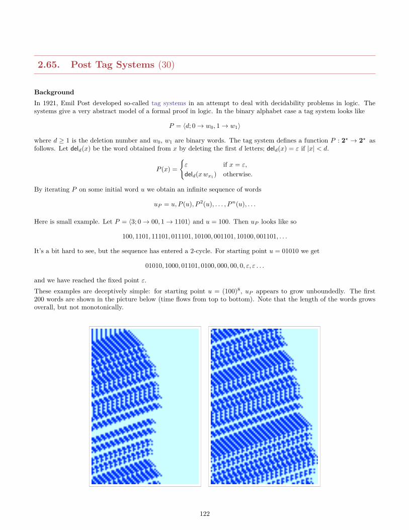
2.65. Post Tag Systems (30)

BackgroundIn 1921, Emil Post developed so-called tag systems in an attempt to deal with decidability problems in logic. Thesystems give a very abstract model of a formal proof in logic. In the binary alphabet case a tag system looks like

P = 〈d; 0→ w0, 1→ w1〉

where d ≥ 1 is the deletion number and w0, w1 are binary words. The tag system defines a function P : 2? → 2? asfollows. Let deld(x) be the word obtained from x by deleting the first d letters; deld(x) = ε if |x| < d.

P (x) =ε if x = ε,deld(xwx1) otherwise.

By iterating P on some initial word u we obtain an infinite sequence of words

uP = u, P (u), P 2(u), . . . , Pn(u), . . .

Here is small example. Let P = 〈3; 0→ 00, 1→ 1101〉 and u = 100. Then uP looks like so

100, 1101, 11101, 011101, 10100, 001101, 10100, 001101, . . .

It’s a bit hard to see, but the sequence has entered a 2-cycle. For starting point u = 01010 we get

01010, 1000, 01101, 0100, 000, 00, 0, ε, ε . . .

and we have reached the fixed point ε.These examples are deceptively simple: for starting point u = (100)8, uP appears to grow unboundedly. The first200 words are shown in the picture below (time flows from top to bottom). Note that the length of the words growsoverall, but not monotonically.

122

Clearly, all sequences uP must either contain words of unbounded length, or lead to a cycle. A tag system P is said tobe decidable if it is decidable whether uP is cyclic or unbounded, u ∈ 2?. As it turns out, even for a relatively small tagsystem, it can be very difficult to determine its behavior. It was shown in 1961 by Minsky that tag systems are indeedundecidable in general (by showing how to simulate Turing machines as tag systems). This fact has recently beenexploited to construct surprisingly small universal Turing machines. Alas, even for the example system from above,its decidability status is not known (worse, we even don’t know what happens in the specific instance u = (100)8).However, if the deletion number is less than 3 we always have decidability (note that we only deal with binary alphabetshere, larger alphabets are an entirely different story).

TaskTo simplify notation a bit, let us assume by symmetry that l0 = |w0| ≤ |w1| = l1.

A. Show that any tag system 〈1; 0→ w0, 1→ w1〉 is decidable.

B. Show that any tag system 〈2; 0→ ε, 1→ w1〉 is decidable.

C. Show that all orbits of P = 〈2; 0→ 1, 1→ 100〉 are ultimately cyclic (so P is trivially decidable).

D. Show that any tag system is decidable if d ≤ l0 or l1 ≤ d.

CommentThe trick here is to find compact, elegant arguments. It is easy to drown in countless separate cases if one tries tobrute-force this problem (and one is not Emil Post).For the first 3 parts it may be helpful to implement the systems to get a feeling for what the orbits uP look like.

123

Chapter 3

Induction, Iteration

124

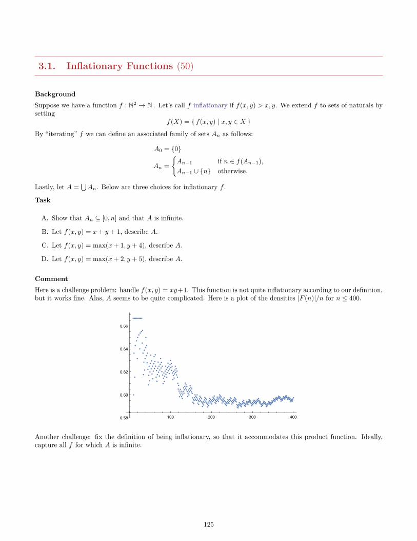
3.1. Inflationary Functions (50)

BackgroundSuppose we have a function f : N2 → N . Let’s call f inflationary if f(x, y) > x, y. We extend f to sets of naturals bysetting

f(X) = f(x, y) | x, y ∈ X

By “iterating” f we can define an associated family of sets An as follows:

A0 = 0

An =An−1 if n ∈ f(An−1),An−1 ∪ n otherwise.

Lastly, let A =⋃An. Below are three choices for inflationary f .

Task

A. Show that An ⊆ [0, n] and that A is infinite.

B. Let f(x, y) = x+ y + 1, describe A.

C. Let f(x, y) = max(x+ 1, y + 4), describe A.

D. Let f(x, y) = max(x+ 2, y + 5), describe A.

CommentHere is a challenge problem: handle f(x, y) = xy+1. This function is not quite inflationary according to our definition,but it works fine. Alas, A seems to be quite complicated. Here is a plot of the densities |F (n)|/n for n ≤ 400.

100 200 300 4000.58

0.60

0.62

0.64

0.66

Another challenge: fix the definition of being inflationary, so that it accommodates this product function. Ideally,capture all f for which A is infinite.

125

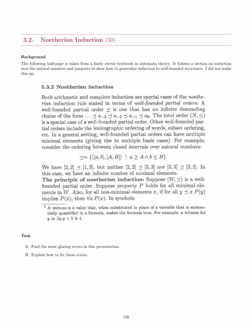
3.2. Noetherian Induction (50)

BackgroundThe following half-page is taken from a fairly recent textbook in automata theory. It follows a section on inductionover the natural numbers and purports to show how to generalize induction to well-founded structures. I did not makethis up.

Task

A. Find the most glaring errors in this presentation.

B. Explain how to fix these errors.

126

3.3. Divisibility (50)

Background

Task

A. Show by induction that n3 + 2n is divisible by 3.

B. Show that n3 − n is divisible by 6, not using induction.

127

3.4. Counting Digits (50)

BackgroundHere is a arithmetic function h that counts digits in the decimal expansion of the input: count the even digits, theodd digits and all digits, and concatenate these counts (all in decimal). In place of a formal definition, here are someexamples: h(1000) = 314, h(22222) = 505, h(1234567890) = 5510.

Task

A. Determine the orbits of n = 1, 12345678910, 10100 − 1 under h.

B. Based on part (A), form a conjecture about the behavior of h and prove your conjecture.

Comment

128

3.5. m-Leaders (50)

BackgroundThe following combinatorial lemma can be used in the proof of a famous theorem in dynamical systems, the so-calledErgodic Theorem. Don’t ask.Suppose A = (a1, . . . , an) is a vector of real numbers of length n. Position i, 1 ≤ i ≤ n, is an m-leader if there is anumber r, 1 ≤ r ≤ m, such that

i+r−1∑j=i

aj ≥ 0

In other words, if we sum up r ≤ m terms in A starting at position i we get a non-negative partial sum. Hence, i is a1-leader iff ai ≥ 0 and i is a 2-leader iff ai ≥ 0 or ai + ai+1 ≥ 0.

Task

A. Let A = (3,−2,−14,−10, 1, 10,−10,−17,−11,−8,−15,−4,−16,−20, 5, 4,−20, 1,−4, 3). Determine the m lead-ers for all m.

B. For all m, the sum of all ai, where i ranges over all m-leaders, is non-negative.

Comment

129

3.6. Inflationary Functions (50)

BackgroundA function f : Nk → N is inflationary if f(x1, . . . , xk) > xi for all i. For A ⊆ N write f(A) to mean f(x1, . . . , xk) |xi ∈ A . Call A splitting if f(A) = N−A.

Task

A. Find a splitting set for f(x) = x+ 1.

B. Find a splitting set for f(x) = max(x+ 1, y + 4).

C. How about f(x, y) = xy + 1?

D. Show that every inflationary function admits a splitting set.

E. Prove or provide a counterexample: this splitting set is uniquely determined by f and is always infinite.

Comment

130

3.7. Spreading Negativity (50)

BackgroundConsider a cyclic sequence of five integers a1, a2, a3, a4 a5. We define an update operation on such sequences asfollows: if a number is negative, add it to its two neighbors, then replace the number itself by its absolute value.For example, 1, 2,−5, 0, 1 would turn into 1,−3, 5,−5, 1. If there are multiple negative numbers we apply the rulein parallel, so the last sequence turns into −2, 3,−3, 5,−4. If there are no negative numbers the sequence does notchange.Let’s refer to the sum a1 + a2 + a3 + a4 + a5 as the weight w(a) of the sequence.

Task

A. Show that all sequences with positive weight will reach a fixed point.

B. Prove or disprove the following conjecture: every starting sequence ultimately winds up in a limit cycle of length1, 2 or 5.

CommentPart (A) is truly annoying: once you see the key idea the rest can be handled by a computer algebra system, butwithout this idea there is little hope. I tend to believe that part (B) is true, but I am not certain (and, of course, Idon’t have a proof).Lastly, note that length 5 is important here; this does not generalize to arbitrary lengths.

131

3.8. Hereditarily Finite Sets (50)

BackgroundA hereditarily finite set is a set this is finite, contains only finite sets which in turn contain only finite sets, and soon. One can think of the collection of all hereditarily finite sets HF as the universe of (finite) combinatorics andcomputability theory (in many ways a better sandbox than N, the set of natural numbers).More formally, define HF to be the smallest set H (with respect to set inclusion) that contains ∅ and such that

x1, . . . , xn ∈ H implies x1, . . . , xn ∈ H.

Here is an alternative way of describing this collection of sets. By induction set P0 = ∅ and Pn+1 = P(Pn) ∪ Pn andlet P =

⋃Pn. As always, P denotes the power set operation.

HF is countable and one can define a particularly simple bijection C : N→ HF as follows. Set

C(n) =∅ if n = 0,C(i) | dig(n, i) = 1 otherwise.

Here dig(n, i) denotes the ith digit of n in the standard binary expansion, 0-indexed with the LSD in position 0.

Task

A. Show that P = HF.

B. Show that C is a bijection.

C. Give a reasonable description of C−1.

Comment

132

3.9. Inverse Sequences (50)

BackgroundOne tool in the study of the sequence of primes 2, 3, 5, 7, 11, 13, 17, 19, 23, 29, . . . is the function counting the numberof primes less than a given positive integer: 0, 1, 2, 2, 3, 3, 4, 4, 4, 4, . . .. Of course, the two sequences are very closelyrelated: given the sequence of primes we can produce the counting sequence, and conversely.More generally, suppose f : N+ → N is non-decreasing and unbounded function. Define the associated countingfunction f? by

f?(x) = number of z : f(z) < x

Two functions f and g on the positive integers are complementary if, for all pairs m and n of positive integers

f(m) < n xor g(n) < m.

Task

A. Show that f? is also non-decreasing and unbounded.

B. Show that the map f 7→ f? is injective.

C. Show that f and f? are complementary whenever f is non-decreasing and unbounded.

D. Determine f?? for a few examples such as the identity function, squares, Fibonacci numbers and the like. Forma conjecture as to what f?? is in general, and prove you conjecture.

133

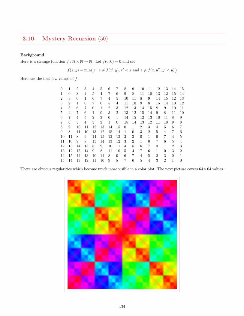
3.10. Mystery Recursion (50)

BackgroundHere is a strange function f : N× N→ N . Let f(0, 0) = 0 and set

f(x, y) = min(z | z 6= f(x′, y), x′ < x and z 6= f(x, y′), y′ < y)

)Here are the first few values of f .

0 1 2 3 4 5 6 7 8 9 10 11 12 13 14 151 0 3 2 5 4 7 6 9 8 11 10 13 12 15 142 3 0 1 6 7 4 5 10 11 8 9 14 15 12 133 2 1 0 7 6 5 4 11 10 9 8 15 14 13 124 5 6 7 0 1 2 3 12 13 14 15 8 9 10 115 4 7 6 1 0 3 2 13 12 15 14 9 8 11 106 7 4 5 2 3 0 1 14 15 12 13 10 11 8 97 6 5 4 3 2 1 0 15 14 13 12 11 10 9 88 9 10 11 12 13 14 15 0 1 2 3 4 5 6 79 8 11 10 13 12 15 14 1 0 3 2 5 4 7 610 11 8 9 14 15 12 13 2 3 0 1 6 7 4 511 10 9 8 15 14 13 12 3 2 1 0 7 6 5 412 13 14 15 8 9 10 11 4 5 6 7 0 1 2 313 12 15 14 9 8 11 10 5 4 7 6 1 0 3 214 15 12 13 10 11 8 9 6 7 4 5 2 3 0 115 14 13 12 11 10 9 8 7 6 5 4 3 2 1 0

There are obvious regularities which become much more visible in a color plot. The next picture covers 64×64 values.

134

Task

A. Show that f is symmetric, that f(x, 0) = x = f(0, x) and that f(x, x) = 0.

B. Give a simple closed form for f(x, y).

CommentFor the second part it may be a good idea to ignore the definition of f for a while and focus on the picture. Recallthat it shows the values of f(x, y) for 0 ≤ x, y < 64 and describe the recursive structure via a simple function of x andy. Then show that the new function is equivalent to f .

135

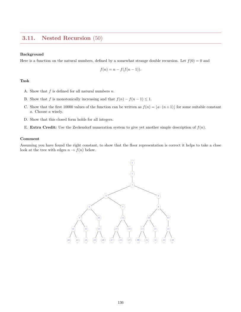
3.11. Nested Recursion (50)

BackgroundHere is a function on the natural numbers, defined by a somewhat strange double recursion. Let f(0) = 0 and

f(n) = n− f(f(n− 1)).

Task

A. Show that f is defined for all natural numbers n.

B. Show that f is monotonically increasing and that f(n)− f(n− 1) ≤ 1.

C. Show that the first 10000 values of the function can be written as f(n) = ba · (n+ 1)c for some suitable constanta. Choose a wisely.

D. Show that this closed form holds for all integers.

E. Extra Credit: Use the Zeckendorf numeration system to give yet another simple description of f(n).

CommentAssuming you have found the right constant, to show that the floor representation is correct it helps to take a closelook at the tree with edges n→ f(n) below.

136

3.12. Powers of Two (50)

Background Let m < n be two positive integers. Recall that ν2(x) denotes the maximum k such that 2k dividesx.

Claim: The interval [m,n] contains a unique element that maximizes ν2.

Task

A. Prove the claim.

B. Give an efficient algorithm that computes this unique element, given m and n.

C. What is the time complexity of your algorithm?

137

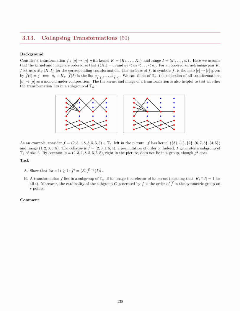
3.13. Collapsing Transformations (50)

BackgroundConsider a transformation f : [n] → [n] with kernel K = (K1, . . . ,Kr) and range I = (a1, . . . , ar) . Here we assumethat the kernel and image are ordered so that f(Ki) = ai and a1 < a2 < . . . < ar. For an ordered kernel/image pair K,I let us write 〈K, I〉 for the corresponding transformation. The collapse of f , in symbols f , is the map [r]→ [r] givenby f(i) = j ⇐⇒ ai ∈ Kj . f(I) is the list a

f(1), . . . , af(r). We can think of Tn, the collection of all transformations[n]→ [n] as a monoid under composition. The the kernel and image of a transformation is also helpful to test whetherthe transformation lies in a subgroup of Tn.

As an example, consider f = (2, 3, 1, 8, 8, 5, 5, 5) ∈ T8, left in the picture. f has kernel (3, 1, 2, 6, 7, 8, 4, 5)and image (1, 2, 3, 5, 8). The collapse is f = (2, 3, 1, 5, 4), a permutation of order 6. Indeed, f generates a subgroup ofT8 of size 6. By contrast, g = (2, 3, 1, 8, 5, 5, 5, 5), right in the picture, does not lie in a group, though g2 does.

Task

A. Show that for all t ≥ 1: f t = 〈K, f t−1(I)〉 .

B. A transformation f lies in a subgroup of Tn iff its image is a selector of its kernel (meaning that |Ki ∩ I| = 1 forall i). Moreover, the cardinality of the subgroup G generated by f is the order of f in the symmetric group onr points.

Comment

138

3.14. Reversal and Palindromes (50)

BackgroundDefine the reversal of a word over alphabet Σ inductively as follows.

rev(ε) = ε

rev(xa) = a rev(x)

Here x ∈ Σ?, a ∈ Σ. A word x is a palindrome if x = rev(x).

Task

A. rev(ax) = rev(x) a for all x ∈ Σ?, a ∈ Σ.

B. rev(xy) = rev(y) rev(x) for all x, y ∈ Σ?.

C. All palindromes are of the form w rev(w) or wa rev(w).

D. rev(rev(x)) = x for all x ∈ Σ?.

E. rev(xn) = rev(x)n for all x ∈ Σ?, n ≥ 0.

Comment

139

3.15. Lookup Tables and Iteration (50)

BackgroundSuppose a function f : [n]→ [n] is given as a lookup table, say, a plain array of integers. Assume that n is machine-sized so that f(x) can be determined in O(1) time. In order to determine f t(x) we can use repeated lookup. However,if we need to determine f t(x) repeatedly it is better to perform a pre-computation that augments the table for f . Theenlarged table then allows for speedy lookups of iterated values of the function f .

Task

A. What would you do if f is a permutation?

B. Explain how to augment the table for arbitrary f so that lookups of f t(x) are fast(er).

C. How long does it take in your solution to determine f t(x)?

D. What is the memory requirement for your table?

E. What is the cost of the pre-computation?

Extra Credit: Assume for the moment that for any function f : A→ A it is always true that f t(x) can be computedin O(log t) applications of f . Here A can be any discrete set whatsoever. Use this to wreak havoc on complexitytheory.

140

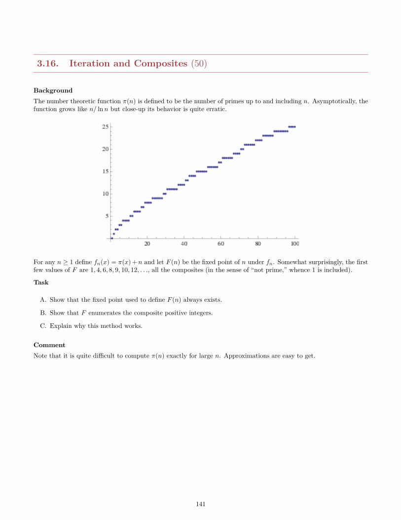
3.16. Iteration and Composites (50)

BackgroundThe number theoretic function π(n) is defined to be the number of primes up to and including n. Asymptotically, thefunction grows like n/ lnn but close-up its behavior is quite erratic.

For any n ≥ 1 define fn(x) = π(x) +n and let F (n) be the fixed point of n under fn. Somewhat surprisingly, the firstfew values of F are 1, 4, 6, 8, 9, 10, 12, . . ., all the composites (in the sense of “not prime,” whence 1 is included).

Task

A. Show that the fixed point used to define F (n) always exists.

B. Show that F enumerates the composite positive integers.

C. Explain why this method works.

CommentNote that it is quite difficult to compute π(n) exactly for large n. Approximations are easy to get.

141

3.17. Fast Exponentiation (50)

BackgroundSeveral classical fast methods to perform fast exponentiation ae where e is a positive integer (and a an element ofsome monoid) are based on squaring:

a2e = sq(ae) a2e+1 = sq(ae) · a

Here are three variants.

// exp1

x = 1;foreach d binary digit of e, MSD first do

x = sq(x);if( d == 1 ) x = a * y;

return x;

// exp2(x,z) = (1,a);foreach d binary digit of e, LSD first do

if( d == 1 ) x = x * z;z = sq(z);

return x;

// exp3(x,z) = (1,a);foreach d binary digit of e, MSD first do

if( d == 1 )(x,z) = ( x * z, sq(z) );

else(x,z) = ( sq(x), x * z );

return x;

Task

A. Show that exp1 correctly computes ae.

B. Show that exp2 correctly computes ae.

C. Show that exp3 correctly computes ae.

D. Compare the performance of the three methods. Distinguish between multiplications and squaring operations.

142

3.18. Greatest Common Divisor (50)

BackgroundThe classical method to compute greatest common divisors of two positive integers is the Euclidean algorithm. Hereare two alternative ways to compute the GCD. The first is slightly non-standard but the second is positively wild.Assume that n and m are positive integers.Here is the first function:

H(n,m) =

m if n = 02H(n/2,m/2) if n, m evenH(n/2,m) if n even, m oddH(n,m/2) if n odd, m evenH((n−m)/2,m) if n, m odd, n ≥ mH(n, (m− n)/2) if n, m odd, n < m

And here is the second:

G(n,m) = 2m−1∑i=1bn imc+ n+m− nm

Task

A. Show that H(n,m) is the GCD of n and m.

B. Show that G(n,m) is the GCD of n and m.

C. Determine the time complexity of both functions.

CommentNote that it absolutely unclear from the definition that G is symmetric. It might help to implement the function andcompute the terms in the summation in a few concrete cases.

143

3.19. Binary Square Roots (50)

BackgroundFor positive integers n define β(n) = binsqr(n, 1) where the latter function is defined by

binsqr( n, s ) if( n < s ) return 0;z = binsqr(n,2*s) + s;return ( z*z <= n ? z : z - s );

Task

A. Show that β(n) = b√nc.

B. What is the time complexity of β (assuming the standard multiplication method).

144

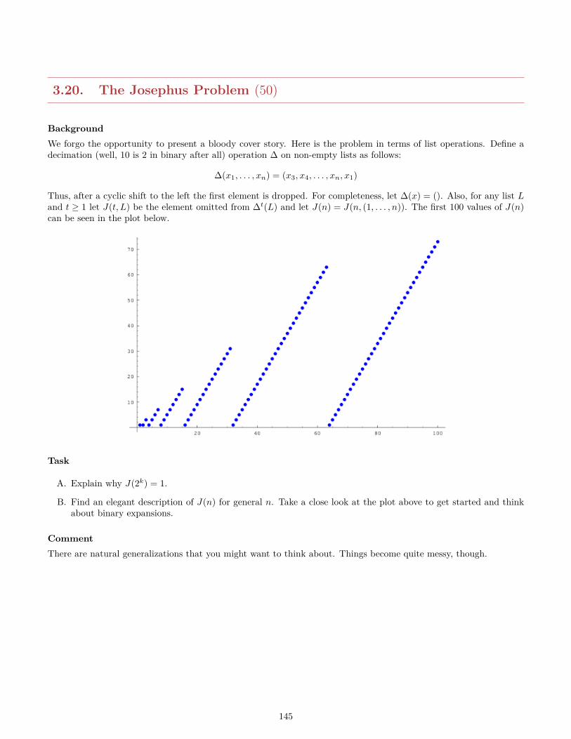
3.20. The Josephus Problem (50)

BackgroundWe forgo the opportunity to present a bloody cover story. Here is the problem in terms of list operations. Define adecimation (well, 10 is 2 in binary after all) operation ∆ on non-empty lists as follows:

∆(x1, . . . , xn) = (x3, x4, . . . , xn, x1)

Thus, after a cyclic shift to the left the first element is dropped. For completeness, let ∆(x) = (). Also, for any list Land t ≥ 1 let J(t, L) be the element omitted from ∆t(L) and let J(n) = J(n, (1, . . . , n)). The first 100 values of J(n)can be seen in the plot below.

Task

A. Explain why J(2k) = 1.

B. Find an elegant description of J(n) for general n. Take a close look at the plot above to get started and thinkabout binary expansions.

CommentThere are natural generalizations that you might want to think about. Things become quite messy, though.

145

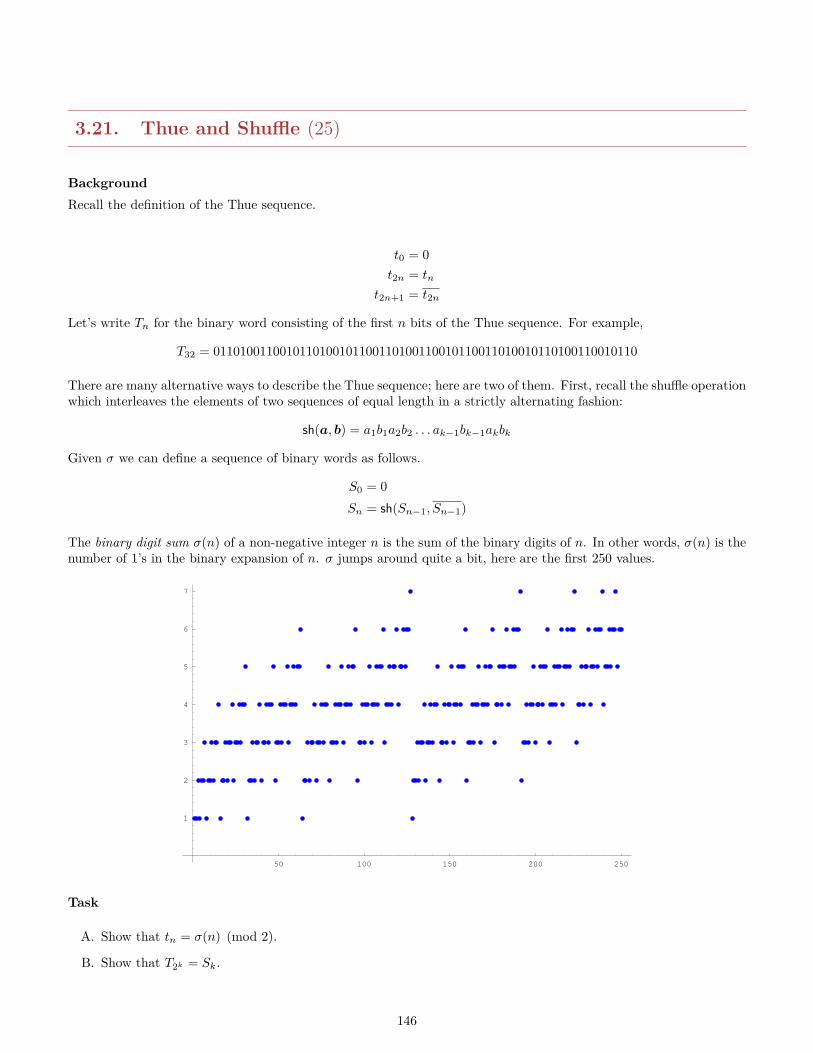
3.21. Thue and Shuffle (25)

BackgroundRecall the definition of the Thue sequence.

t0 = 0t2n = tn

t2n+1 = t2n

Let’s write Tn for the binary word consisting of the first n bits of the Thue sequence. For example,

T32 = 0110100110010110100101100110100110010110011010010110100110010110

There are many alternative ways to describe the Thue sequence; here are two of them. First, recall the shuffle operationwhich interleaves the elements of two sequences of equal length in a strictly alternating fashion:

sh(a, b) = a1b1a2b2 . . . ak−1bk−1akbk

Given σ we can define a sequence of binary words as follows.

S0 = 0Sn = sh(Sn−1, Sn−1)

The binary digit sum σ(n) of a non-negative integer n is the sum of the binary digits of n. In other words, σ(n) is thenumber of 1’s in the binary expansion of n. σ jumps around quite a bit, here are the first 250 values.

50 100 150 200 250

1

2

3

4

5

6

7

Task

A. Show that tn = σ(n) (mod 2).

B. Show that T2k = Sk.

146

3.22. Fibonacci Words (25)

BackgroundThe following recursion defines a collection of binary words, the so-called Fibonacci words.

W0 = ε

W1 = 0W2 = 1Wn = Wn−1Wn−2

The first 10 Fibonacci words are listed in the following table:

0 ε1 02 13 104 1015 101106 101101017 10110101101108 1011010110110101101019 1011010110110101101011011010110110

Needless to say, the lengths of the Fibonacci lists are just the Fibonacci numbers. Note that W2n = . . . 01 and W2n+1 =. . . 10 for n ≥ 2. For any word of length at least 2 define σ(x1x2 . . . xk−1xk) to be the word x1x2 . . . xk−2xkxk−1. Letδ(x1x2 . . . xk−1xk) = x1x2 . . . xk−2. Thus operation σ swaps the last 2 letters of a word while σ removes the last 2letters.

Task

A. Show that Wn = σ(Wn−2Wn−1) for all n ≥ 3.

B. Show that δ(Wn) is a palindrome for all n ≥ 4.

147

3.23. Mycielski Graphs (25)

BackgroundLet G = 〈V,E〉 be an undirected graph. The Mycielski graph µ(G) has vertex set V ∪ V ∪ > where V is a disjointcopy of V and > a new vertex. The edges are

E ∪ uv | uv ∈ E ∪ u> | v ∈ V .

These graphs are important in connection with small graphs having a given chromatic number.

TaskLet n be the number of nodes in G and e the number of edges.

A. Let P2 be the graph consisting of one edge. Draw µ2(P2).

B. Find a closed form for the size of the vertex set of µk(G).

C. Find a closed form for the size of the edge set of µk(G).

148

3.24. Tournaments and Kings (25)

BackgroundA tournament is a random orientation on a complete graph: We interpret edge x → y to mean that x beats y. Calla node v a king if for any node x there is a path from v to x of length at most 2. A royal tournament is one whereeverybody is a king. A champion is any node with maximal out-degree: a player with the maximal number of wins.Hence champions trivially exist, though they are not unique in general. It is not clear that kings exist in general.

Claim: Every tournament has a king.

Task

A. Prove the claim by induction on the number of nodes.

B. Prove the claim by showing that every champion is a king.

C. Show that a royal tournament of size n exists if, and only if, n 6= 2, 4.

149

3.25. Tournaments and Fairness (25)

BackgroundA tournament is a random orientation on a complete graph: We interpret edge x→ y to mean that x beats y. Supposethe tournament has vertex set V and size n. By a ranking we mean a function r : V → [n] . Intuitively, a ranking isfair if whenever there is a path from p to q then p is higher ranked: r(p) < r(q). Alas, tournaments may well containcycles: “beats” is not a transitive relation and so in general we cannot construct fair rankings. Call a ranking 1-fairif r(p) = r(q) + 1 implies that q beat p.

Task

A. Show how to construct a fair ranking in linear time for any acyclic tournament.

B. Show that any tournament that contains a cycle of length at least 3 also contains a cycle of length exactly 3.

C. Show that every tournament admits a 1-fair ranking.

CommentThe second part is tricky; use induction on the number of nodes to show the stronger claim that the top-ranked nodecan always be chosen to be a champion (maximum number of wins).

150

3.26. Ducci Sequences (50)

BackgroundRecall the Ducci sequences introduced in class: iterate the function

D(x1, x2, x3, x4) = (|x1 − x2|, |x2 − x3|, |x3 − x4|, |x4 − x1|)

on N4. A typical orbit looks like so:

0 94 68 11 851 26 57 74 92 31 17 65 173 14 48 48 144 34 0 34 05 34 34 34 346 0 0 0 0

Task

A. Explain how to use the tribonacci numbers

tn = tn−1 + tn−2 + tn−3 t0 = t1 = 0 t2 = 1

to show that the transients (leading to fixed point 0) can be arbitrarily long.

B. Prove that every Ducci sequence ends in fixed point 0. We are only dealing with vectors of length 4 here.

CommentYou probably want to write a little program and print out some orbits of tribonacci Ducci-orbits; ponder deeply anda conjecture will jump out at you. Even with the right conjecture the proof is a bit tedious. Try to come up with acrisp, elegant argument.Extra credit: Generalize the second claim to any initial vector of length 2k.

151

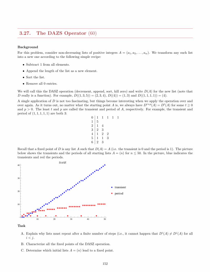
3.27. The DAZS Operator (60)

BackgroundFor this problem, consider non-decreasing lists of positive integers A = (a1, a2, . . . , aw). We transform any such listinto a new one according to the following simple recipe:

• Subtract 1 from all elements.

• Append the length of the list as a new element.

• Sort the list.

• Remove all 0 entries.

We will call this the DASZ operation (decrement, append, sort, kill zero) and write D(A) for the new list (note thatD really is a function). For example, D((1, 3, 5)) = (2, 3, 4), D((4)) = (1, 3) and D((1, 1, 1, 1)) = (4).A single application of D is not too fascinating, but things become interesting when we apply the operation over andover again. As it turns out, no matter what the starting point A is, we always have Dt+p(A) = Dt(A) for some t ≥ 0and p > 0. The least t and p are called the transient and period of A, respectively. For example, the transient andperiod of (1, 1, 1, 1, 1) are both 3:

0 1 1 1 1 11 52 1 43 2 34 1 2 25 1 1 36 2 3

Recall that a fixed point of D is any list A such that D(A) = A (i.e. the transient is 0 and the period is 1). The picturebelow shows the transients and the periods of all starting lists A = (n) for n ≤ 50. In the picture, blue indicates thetransients and red the periods.

Task

A. Explain why lists must repeat after a finite number of steps (i.e., it cannot happen that Di(A) 6= Dj(A) for alli < j.

B. Characterize all the fixed points of the DASZ operation.

C. Determine which initial lists A = (n) lead to a fixed point.

152

CommentYou might find it useful to compute a few more examples. Needless to say, it is not enough to merely state the answers,you have to prove that your claim is correct.

153

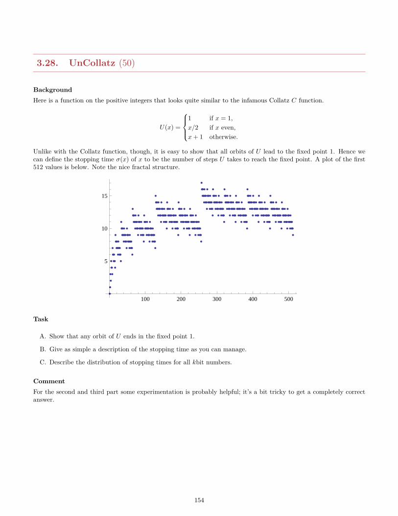
3.28. UnCollatz (50)

BackgroundHere is a function on the positive integers that looks quite similar to the infamous Collatz C function.

U(x) =

1 if x = 1,x/2 if x even,x+ 1 otherwise.

Unlike with the Collatz function, though, it is easy to show that all orbits of U lead to the fixed point 1. Hence wecan define the stopping time σ(x) of x to be the number of steps U takes to reach the fixed point. A plot of the first512 values is below. Note the nice fractal structure.

100 200 300 400 500

5

10

15

Task

A. Show that any orbit of U ends in the fixed point 1.

B. Give as simple a description of the stopping time as you can manage.

C. Describe the distribution of stopping times for all kbit numbers.

CommentFor the second and third part some experimentation is probably helpful; it’s a bit tricky to get a completely correctanswer.

154

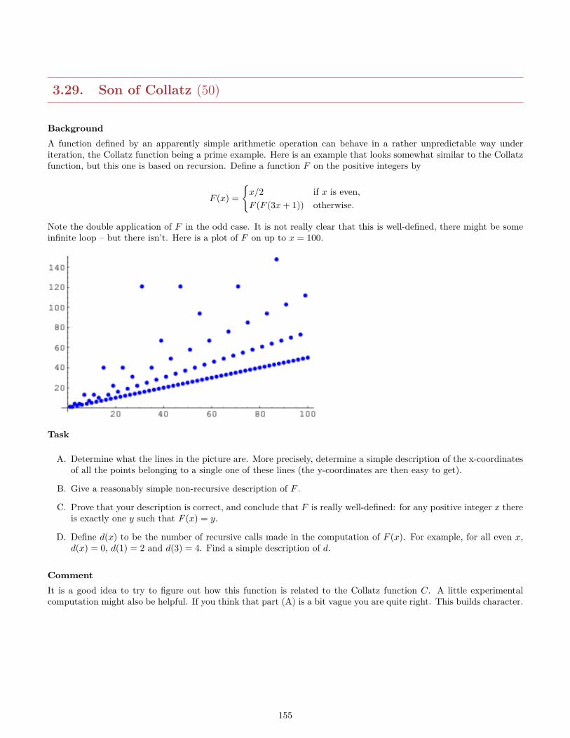
3.29. Son of Collatz (50)

BackgroundA function defined by an apparently simple arithmetic operation can behave in a rather unpredictable way underiteration, the Collatz function being a prime example. Here is an example that looks somewhat similar to the Collatzfunction, but this one is based on recursion. Define a function F on the positive integers by

F (x) =x/2 if x is even,F (F (3x+ 1)) otherwise.

Note the double application of F in the odd case. It is not really clear that this is well-defined, there might be someinfinite loop – but there isn’t. Here is a plot of F on up to x = 100.

Task

A. Determine what the lines in the picture are. More precisely, determine a simple description of the x-coordinatesof all the points belonging to a single one of these lines (the y-coordinates are then easy to get).

B. Give a reasonably simple non-recursive description of F .

C. Prove that your description is correct, and conclude that F is really well-defined: for any positive integer x thereis exactly one y such that F (x) = y.

D. Define d(x) to be the number of recursive calls made in the computation of F (x). For example, for all even x,d(x) = 0, d(1) = 2 and d(3) = 4. Find a simple description of d.

CommentIt is a good idea to try to figure out how this function is related to the Collatz function C. A little experimentalcomputation might also be helpful. If you think that part (A) is a bit vague you are quite right. This builds character.

155

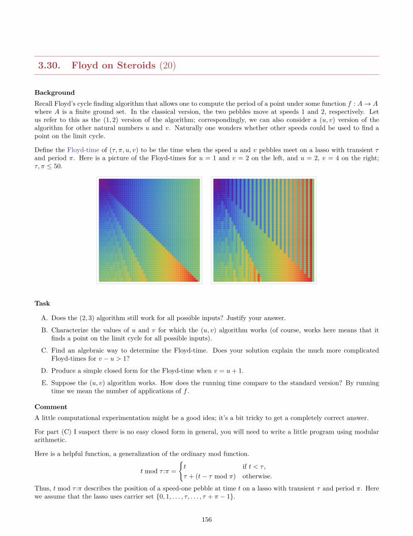
3.30. Floyd on Steroids (20)

BackgroundRecall Floyd’s cycle finding algorithm that allows one to compute the period of a point under some function f : A→ Awhere A is a finite ground set. In the classical version, the two pebbles move at speeds 1 and 2, respectively. Letus refer to this as the (1, 2) version of the algorithm; correspondingly, we can also consider a (u, v) version of thealgorithm for other natural numbers u and v. Naturally one wonders whether other speeds could be used to find apoint on the limit cycle.

Define the Floyd-time of (τ, π, u, v) to be the time when the speed u and v pebbles meet on a lasso with transient τand period π. Here is a picture of the Floyd-times for u = 1 and v = 2 on the left, and u = 2, v = 4 on the right;τ, π ≤ 50.

Task

A. Does the (2, 3) algorithm still work for all possible inputs? Justify your answer.

B. Characterize the values of u and v for which the (u, v) algorithm works (of course, works here means that itfinds a point on the limit cycle for all possible inputs).

C. Find an algebraic way to determine the Floyd-time. Does your solution explain the much more complicatedFloyd-times for v − u > 1?

D. Produce a simple closed form for the Floyd-time when v = u+ 1.

E. Suppose the (u, v) algorithm works. How does the running time compare to the standard version? By runningtime we mean the number of applications of f .

CommentA little computational experimentation might be a good idea; it’s a bit tricky to get a completely correct answer.

For part (C) I suspect there is no easy closed form in general, you will need to write a little program using modulararithmetic.

Here is a helpful function, a generalization of the ordinary mod function.

t mod τ :π =t if t < τ ,τ + (t− τ mod π) otherwise.

Thus, t mod τ :π describes the position of a speed-one pebble at time t on a lasso with transient τ and period π. Herewe assume that the lasso uses carrier set 0, 1, . . . , τ, . . . , τ + π − 1.

156

3.31. Floyd and Teleportation (50)

BackgroundRecall Floyd’s trick to determine the transient and period of a finite orbit without using extra memory: two pebblesmove at speeds 1 and 2 , respectively. Here is a modification of this approach where the “slow” pebble does not moveat all, except that it occasionally teleports to the location of the “fast” pebble.Here is the crucial first part of the algorithm that computes the period of the orbit. The function in question is f andthe starting point is a.

slow = a;fast = f(a);per = bnd = 1;while( fast != slow )

if( per == bnd ) slow = fast; per = 0; bnd *= 2;

fast = f(fast);per++;

return per;

The claim is that this algorithm finds a point on the limit cycle. In a separate procedure one can then compute thetransient (just as in Floyd’s method).

Task

A. Prove that upon termination the pebbles are located on some position on the limit cycle. Conclude that thereturn value is indeed the period of the orbit.

B. Determine the time complexity of the teleportation algorithm (i.e., count the number of times the loop isexecuted).

C. Now consider the task of computing both transient and period. Compare the performance of Floyd’s classicalalgorithm and the teleportation algorithm. Is one better than the other? Why?

CommentThis method is due to R. Brent.

157

3.32. Schroder-Bernstein (50)

BackgroundSuppose f : A→ B and g : B → A are two injective functions. Define

A0 = AAn+1 = g(Bn)B0 = BBn+1 = f(An)

and let Aω =⋂An.

Task

A. Explain the sets A2n −A2n+1 and Aω.

B. Define a new function h : A→ B by

h(x) =f(x) if x ∈ Aω or x ∈ A2n −A2n+1,g−1(x) otherwise.

Show that h is a bijection.

Comment

158

3.33. Cardinalities (50)

BackgroundFor the following problem you should rely on the Schroder-Bernstein theorem rather than trying to construct bijectionsdirectly.

Task

A. Show that the real intervals [0, 3], [0, 2) and (0, 1) all have the same cardinality.

B. Show that |2ω| = |ωω|.

Comment

159

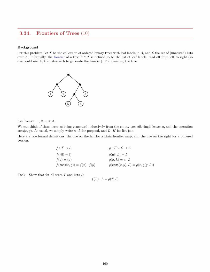
3.34. Frontiers of Trees (10)

BackgroundFor this problem, let T be the collection of ordered binary trees with leaf labels in A, and L the set of (unnested) listsover A. Informally, the frontier of a tree T ∈ T is defined to be the list of leaf labels, read off from left to right (soone could use depth-first-search to generate the frontier). For example, the tree

1 2

5 4

3

has frontier: 1, 2, 5, 4, 3.We can think of these trees as being generated inductively from the empty tree nil, single leaves a, and the operationcons(x, y). As usual, we simply write a · L for prepend, and L ·K for list join.Here are two formal definitions, the one on the left for a plain frontier map, and the one on the right for a bufferedversion.

f : T → L g : T × L → L

f(nil) = () g(nil, L) = L

f(a) = (a) g(a, L) = a · Lf(cons(x, y)) = f(x) · f(y) g(cons(x, y), L) = g(x, g(y, L))

Task Show that for all trees T and lists L:f(T ) · L = g(T, L)

160

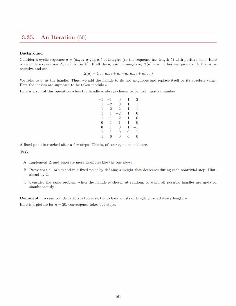
3.35. An Iteration (50)

BackgroundConsider a cyclic sequence a = (a0, a1, a2, a3, a4) of integers (so the sequence has length 5) with positive sum. Hereis an update operation ∆, defined on Z5. If all the ai are non-negative, ∆(a) = a. Otherwise pick i such that ai isnegative and set

∆(a) = (. . . , ai−1 + ai,−ai, ai+1 + ai, . . .)

We refer to ai as the handle. Thus, we add the handle to its two neighbors and replace itself by its absolute value.Here the indices are supposed to be taken modulo 5.Here is a run of this operation when the handle is always chosen to be first negative number:

−1 −1 0 1 21 −2 0 1 1−1 2 −2 1 1

1 1 −2 1 01 −1 2 −1 00 1 1 −1 00 1 0 1 −1−1 1 0 0 1

1 0 0 0 0

A fixed point is reached after a few steps. This is, of course, no coincidence.

Task

A. Implement ∆ and generate more examples like the one above.

B. Prove that all orbits end in a fixed point by defining a weight that decreases during each nontrivial step. Hint:ahead by 2.

C. Consider the same problem when the handle is chosen at random, or when all possible handles are updatedsimultaneously.

Comment In case you think this is too easy, try to handle lists of length 6, or arbitrary length n.Here is a picture for n = 20, convergence takes 699 steps.

161

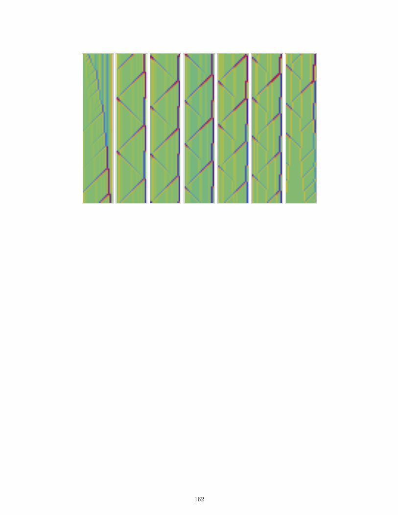
162

3.36. Coinduction (50)

BackgroundFor this problem consider the set Aω of infinite sequences over some ground set A. Given a sequence a = (ai)i≥0 =a0, a1, a2, . . . we write hd(a) = a0 and tl(a) = a1, a2, . . . so that a = hd(a) :: tl(a).Also define the even and odd subsequences by even(a) = a0, a2, a4, . . . and odd(a) = a1, a3, a5, . . .. Lastly, perfectshuffle here means shf(a, b) = a0, b0, a1, b1, . . ..A bisimulation R is a binary relation on Aω such that R(x, y) implies hd(x) = hd(y) and R(tl(x), tl(y)). The coinductiveproof principle says that for any two sequences x and y, if there is a bisimulation R such that R(x, y), then we alreadyhave x = y.

Task

A. Find an equational characterization of shuffle, even and odd that avoids the informal definition from above. Forexample, odd(x) = even(tl(x)).

B. Use your equations to show that shf(even(x), odd(x)) = x.

C. Give another proof of this identity using the coinductive proof principle.

D. Give a proof of the coinductive proof principle.

Comment This is a veritable tip of an iceberg; one can develop a whole theory of coinduction that is nearly asuseful in CS as ordinary induction.

163

—————————————————————————

164

Chapter 4

Algebra

165

4.1. Indecomposable Matrices (50)

BackgroundConsider the monoid Nd of all matrices in Nd×d with determinant 1. A matrix U in Nd is a unit if there is somematrix V such that UV = I. Call a matrix M decomposable if it is a unit, or, for some A and B, M = AB whereneither A nor B is a unit. Lastly, define the following family of matrices in N3:

Mn =

1 0 n1 n−1 01 1 n−1

Task

A. Find a generator for all the units in N3. In general, what do the units in Nd look like?

B. Let Mn = AB. Show that the first row of A can safely be assumed to be of the form (a, 0, 0) or (a, 0, b) wherea, b 6= 0.

C. Show that the matrices M1 and M2 are decomposable.

D. On the other hand, show that all the matrices Mn for n ≥ 3 are indecomposable.

E. By contrast, prove that N2 is isomorphic to the free semigroup over a, b.

CommentFor part (C), consider the case where the first row of A is e1. You might want to tackle the last part first and figureout where the argument fails for n = 1, 2. My argument is kind of hacky, try to come up with an elegant solution.For the last part, come up with two “small” matrices corresponding to a and b.

166

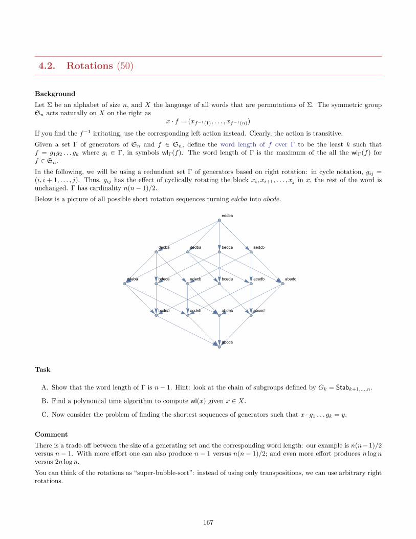
4.2. Rotations (50)

BackgroundLet Σ be an alphabet of size n, and X the language of all words that are permutations of Σ. The symmetric groupSn acts naturally on X on the right as

x · f = (xf−1(1), . . . , xf−1(n))

If you find the f−1 irritating, use the corresponding left action instead. Clearly, the action is transitive.Given a set Γ of generators of Sn and f ∈ Sn, define the word length of f over Γ to be the least k such thatf = g1g2 . . . gk where gi ∈ Γ, in symbols wlΓ(f). The word length of Γ is the maximum of the all the wlΓ(f) forf ∈ Sn.In the following, we will be using a redundant set Γ of generators based on right rotation: in cycle notation, gij =(i, i + 1, . . . , j). Thus, gij has the effect of cyclically rotating the block xi, xi+1, . . . , xj in x, the rest of the word isunchanged. Γ has cardinality n(n− 1)/2.Below is a picture of all possible short rotation sequences turning edcba into abcde.

edcba

decba cedba bedca aedcb

cdeba bdeca adecb bceda acedb abedc

bcdea acdeb abdec abced

abcde

Task

A. Show that the word length of Γ is n− 1. Hint: look at the chain of subgroups defined by Gk = Stabk+1,...,n.

B. Find a polynomial time algorithm to compute wl(x) given x ∈ X.

C. Now consider the problem of finding the shortest sequences of generators such that x · g1 . . . gk = y.

CommentThere is a trade-off between the size of a generating set and the corresponding word length: our example is n(n−1)/2versus n − 1. With more effort one can also produce n − 1 versus n(n − 1)/2; and even more effort produces n lognversus 2n logn.You can think of the rotations as “super-bubble-sort”: instead of using only transpositions, we can use arbitrary rightrotations.

167

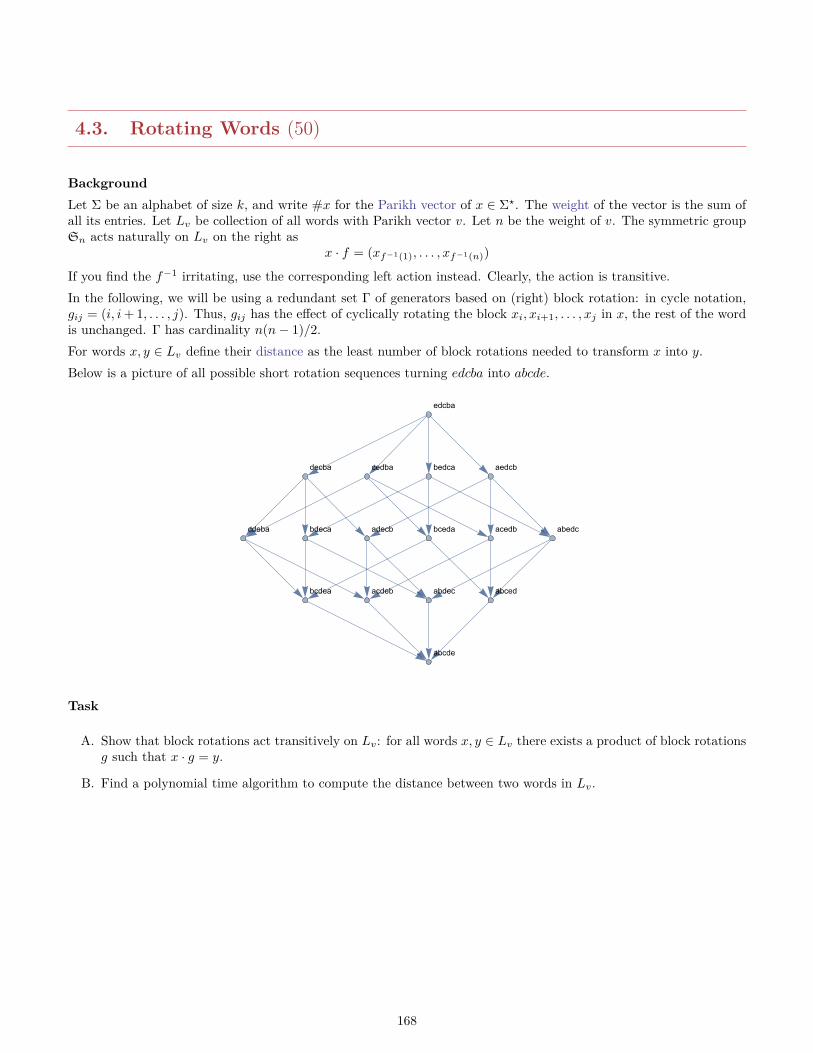
4.3. Rotating Words (50)

BackgroundLet Σ be an alphabet of size k, and write #x for the Parikh vector of x ∈ Σ?. The weight of the vector is the sum ofall its entries. Let Lv be collection of all words with Parikh vector v. Let n be the weight of v. The symmetric groupSn acts naturally on Lv on the right as

x · f = (xf−1(1), . . . , xf−1(n))

If you find the f−1 irritating, use the corresponding left action instead. Clearly, the action is transitive.In the following, we will be using a redundant set Γ of generators based on (right) block rotation: in cycle notation,gij = (i, i+ 1, . . . , j). Thus, gij has the effect of cyclically rotating the block xi, xi+1, . . . , xj in x, the rest of the wordis unchanged. Γ has cardinality n(n− 1)/2.For words x, y ∈ Lv define their distance as the least number of block rotations needed to transform x into y.Below is a picture of all possible short rotation sequences turning edcba into abcde.

edcba

decba cedba bedca aedcb

cdeba bdeca adecb bceda acedb abedc

bcdea acdeb abdec abced

abcde

Task

A. Show that block rotations act transitively on Lv: for all words x, y ∈ Lv there exists a product of block rotationsg such that x · g = y.

B. Find a polynomial time algorithm to compute the distance between two words in Lv.

168

4.4. Subgroups and Counting (50)

BackgroundLet G be a finite group and A 6= ∅ a subset (not necessarily a subgroup). A is said to be symmetric if A−1 = A whereA−1 = a−1 | a ∈ A .

TaskShow that the following are equivalent:

A. A is a subgroup.

B. A is closed under multiplication: A2 ⊆ A.

C. A is symmetric, contains 1 and |A2| = |A|.

D. A contains 1 and A2 = Aa for some a ∈ G.

169

4.5. Matrix Products (50)

BackgroundConsider the two pairs (A0, A1) and (B0, B1) of integer matrices defined by

Ai =(

2 0i 1

)Bi =

(2 0

i+ 1 1

)where i = 0, 1.

Task

A. Find a simple closed form for a product X = X1 · . . . ·Xn where Xi ∈ A0, A1.

B. Conclude that n and the factors Xi can be recovered from the product X.

C. Repeat parts (A) and (B) for Bi instead of Ai.

D. Generalize to more than 2 matrices.

170

4.6. Fibonacci Monoid (50)

BackgroundAs always, we write Fn for the nth Fibonacci number defined by the recurrence: F0 = 0, F1 = 1, Fn = Fn−1 + Fn−2.The obvious iterative approach to computing Fn takes O(n) arithmetic operations. The question is whether one cando better than that.Consider the following operation defined on N× N by the binary operation

(a, b)⊕ (c, d) = (ac+ ad+ bc, ac+ bd)

Define 0 = (1, 0) and 1 = (0, 1) and let M ⊆ N× N be the closure of 1 under this operation.

Task

A. Compute the first 20 elements of this closure. Observations?

B. Show that M is a commutative monoid with neutral element 0.

C. Find a way to extend M to a group G. In particular specify the “minus” and “subtraction” operations.

D. Explain how the monoid can be used to compute Fibonacci numbers quickly.

E. Explain how the group can be used to compute Fibonacci numbers even more quickly, at least sometimes.

171

4.7. Affine Maps (50)

BackgroundWe consider linear functions on the real numbers of the form fa,b(x) = a · x+ b where 0 < a and b arbitrary. We willwrite F for the collection of all such functions.Of course, we can compose these functions according to (f g)(x) = f(g(x)).

Task

A. Show that composition is a binary operation on F: for any two functions f and g in F, f g is again in F.

B. Show that F is a group with respect to .

C. Is the group from part (B) commutative? Justify your answer.

D. We used the condition 0 < a. Can we still get a group if we drop this condition?

172

4.8. Normal Subgroups (50)

BackgroundAn ordinary subgroup H of a group G is a subset of G that satisfies the following properties: 1 ∈ H, x, y ∈ H impliesx · y ∈ H, x ∈ H implies x−1 ∈ H.For an arbitrary subset H we can define a binary relation ∼H on G as follows: x ∼H y iff x·y−1 ∈ H.To lighten notation, we drop the subscript whenever possible.The relation ∼H is actually an equivalence relation. One might wonder whether it is possible to extend the groupoperation to the equivalence classes. The obvious definition is [x] · [y] = [x ·y] which is exactly how we defined additionand also multiplication modulo m. The problem is that we have to check that this operation is well-defined: we needx ∼ u and y ∼ v implies x · y ∼ u · v. Any equivalence relation that satisfies this property is called a congruence.Unfortunately, not every subgroup H gives rise to a congruence ∼H , though we always get an equivalence relation.The subgroups that work a the so-called normal subgroups which have the additional property x ·H = H ·x. Note thatin a commutative group every subgroup is automatically normal. But in non-commutative groups we often encounternon-normal subgroups.

Task

A. Show that H is a subgroup if, and only if, the relation ∼H is an equivalence relation.

B. Show that H is a normal subgroup if, and only if, the relation ∼H is a congruence relation.

173

4.9. Modular Multiplication (50)

BackgroundGiven a modulus m, the numbers coprime with m form a group under multiplication modulo m, the so-called mul-tiplicative subgroup. This group Z?m appears often in number theory and combinatorics; the map Φ(m) = |Z?m| isknown as Euler’s totient function.While Z?m is the most important group of modular numbers under multiplication there are others. For example,3, 9, 21, 27 forms a group for m = 30 with 21 as the unit. We will call any group G ⊆ 1, 2, . . . ,m−1 with modularmultiplication as operation a strange multiplicative group. The key to identifying these strange groups is a simpleobservation: the unit element e of G must be idempotent: e2 = e (mod m). To identify the idempotents modulo m itis convenient to consider divisors a of m such that a and m/a are coprime. We will call these prompt divisors. Recallthat by the Chinese Remainder Theorem Zm is isomorphic to Za × Zm/a for any prompt divisor a.

Task

A. Verify that 3, 9, 21, 27 forms a group for m = 30.

B. Give a characterization of idempotents modulo m in terms of the prime factorization of m. Use this to countthe number of idempotents.

C. Show that every idempotent e is the unit of a group Ge = eZ?m.

D. Show that all the Ge are disjoint.

E. Show that for every prompt divisor a of m we have aZ?m = x ∈ Zm | gcd(x,m) = a .

F. Use the last result to give a simpler description of the groups Ge.

G. Determine the order of the groups Ge.

H. Show that every strange group is a subgroup of some Ge.

CommentFermat’s little theorem and Euler’s totient function are helpful for part (B). One can show that every strange groupis a subgroup of some Ge but that requires quite a bit more work.You might find it useful to do a little experimentation with, say, m = 100.

174

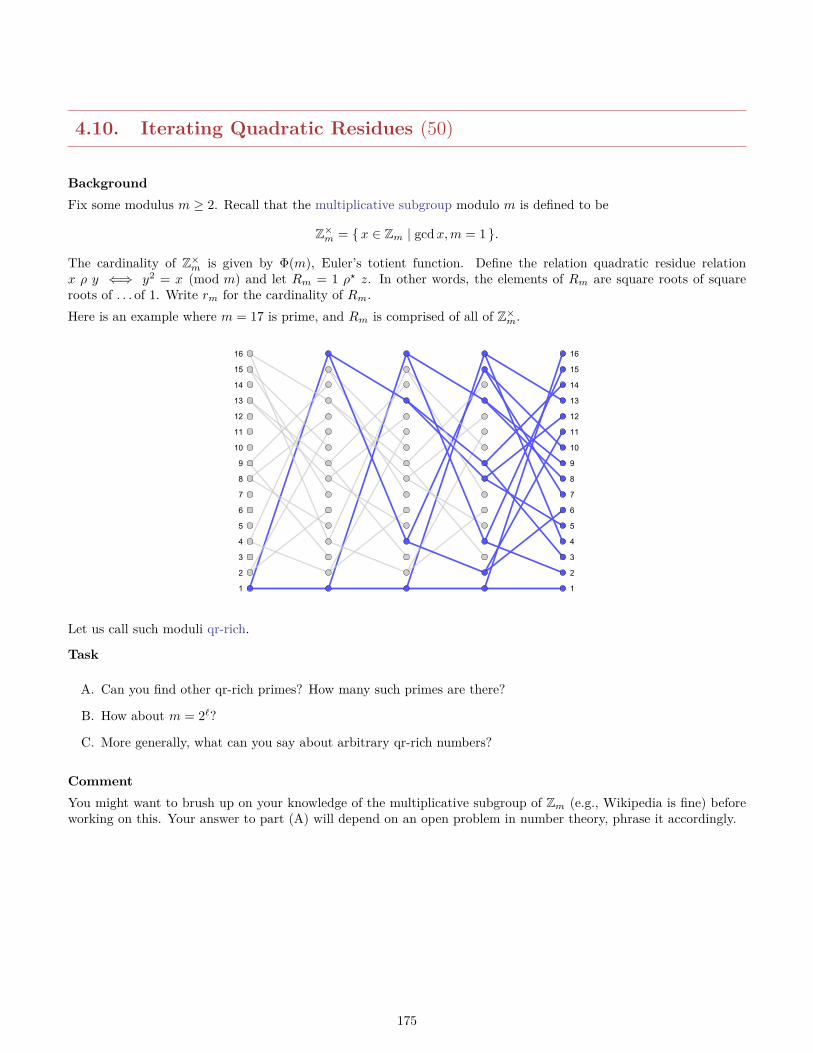
4.10. Iterating Quadratic Residues (50)

BackgroundFix some modulus m ≥ 2. Recall that the multiplicative subgroup modulo m is defined to be

Z×m = x ∈ Zm | gcdx,m = 1 .

The cardinality of Z×m is given by Φ(m), Euler’s totient function. Define the relation quadratic residue relationx ρ y ⇐⇒ y2 = x (mod m) and let Rm = 1 ρ? z. In other words, the elements of Rm are square roots of squareroots of . . . of 1. Write rm for the cardinality of Rm.Here is an example where m = 17 is prime, and Rm is comprised of all of Z×m.

1

2

3

4

5

6

7

8

9

10

11

12

13

14

15

16

1

2

3

4

5

6

7

8

9

10

11

12

13

14

15

16

Let us call such moduli qr-rich.

Task

A. Can you find other qr-rich primes? How many such primes are there?

B. How about m = 2`?

C. More generally, what can you say about arbitrary qr-rich numbers?

CommentYou might want to brush up on your knowledge of the multiplicative subgroup of Zm (e.g., Wikipedia is fine) beforeworking on this. Your answer to part (A) will depend on an open problem in number theory, phrase it accordingly.

175

4.11. An Associative Operation (50)

BackgroundMany operations in algebra are clearly associative. However, in some cases associativity is far from obvious andrequires a proof.For this problem, write [x] for the integer nearest to x ∈ R. More precisely, let [x] = bx + 1/2c so that [3.5] = 4.Consider the map π : N× N→ N defined by

π(x, y) =x+ y2 if x 6= max(x, y),x(x+ 1) + y otherwise.

We can think of the last map is a bijection between N and the first quadrant in the (discrete) plane Z × Z, see part(A). Here is a slightly different map: ρ : N→ N× Z

ρ(x) = ([√x], x− [

√x]2)

Let W ⊆ N× Z be the range of ρ.

A. Show that π is a bijection and determine the unpairing functions.

B. Determine W , the range of ρ and show that ρ is a bijection between N and W .

C. Show that the binary operation on N defined by

a ∗ b = a+ b+ 2[√a][√b]

is associative.

CommentPart (A) is just a warm-up, but part (B) is useful for (C). The latter can also be handled by brute force, but that’s amess.

176

4.12. Generating Permutations and Functions (50)

BackgroundWe have seen that all permutations of [n] can be obtained from the cyclic shift (2, 3, . . . , n, 1) and the transposition(2, 1, 3, . . . , n) by composition. Needless to say, there are many other generating sets (e.g., the set of all transpositions)and there are quite a few of size 2.

Task

A. Describe some generating sets of size 2 for the group of all permutations of [n]. Are there many of these (forsome reasonable sense of many)?

B. Characterize all possible generating sets of size 3 for the monoid of all functions [n] → [n] assuming all sets ofgenerators of size 2 for the symmetric group are known.

C. Find a small set of generators for the alternating group on n points. You might want to find an analogue to thefact that the full symmetric group is generated by transpositions first.

CommentAs always, “characterize” means that you have to find some condition that holds if, and only if, f , g and h aregenerators for the monoid of all functions. Try to find a simple, elegant condition. Then prove that your conditionreally works.Note that the corresponding problem for general relations (under relational composition) is much more difficult: thereis no fixed size set of generators, and the proof is hard.

177

4.13. Matrices and Words (50)

BackgroundThe collection of all words over the alphabet a, b can be construed as a monoid: the associative operation isconcatenation and the neutral element is ε, the empty word. This monoid, usually written a, b?, is well-known tobe free: given an element x ∈ a, b? there is exactly one way to write it as a product of a’s and b’s.Here is another, more algebraic way to generate the free monoid over two elements. Consider the two integer matrices

A =(

1 01 1

)B =

(1 10 1

)Let M ⊆ N2×2 be the monoid generated by A and B.

Task

A. Show that any matrix in M can be written in precisely one way as a product of A and B.

B. Turn the last result into a decomposition algorithm and discuss its running time.

C. Explain how to represent the free monoid over k > 2 generators in terms of matrices.

D. Show that a 2× 2 matrix over N belongs to M if, ond only if, M had determinant 1.

CommentIn a similar way we can produce the free group with two generators by including the inverse matrices of A and B.

178

4.14. Some Boolean Formulas (30)

BackgroundRecall that a Boolean formula is in 2-CNF if it is in conjunctive normal form and all clauses have exactly two literals.By Vertex Cover we mean the decision version: given an undirected graph G and a bound k, is there a vertex-to-edgecover of G of size k?By Partition we mean the problem of splitting a list of positive integers a = (a1, a2, . . . , an) into two parts that havethe same sum. Assume that the numbers ai are given in binary and are all k-digit.

Task

A. Find a fast algorithm to solve satisfiability for formulae in 2-CNF. What is the running time of your algorithm?

B. Show how to translate an instance (G, k) of Vertex Cover into a Boolean formula Φ such that G has a vertexcover of size k iff Φ is satisfiable. What is the size of your formula as a function of the number of n of verticesand the number m of edges (you may assume k ≤ n)?

C. Show how to translate an instance a of Partition into a Boolean formula Φ such that there exists a partitioninto two equal-sum parts iff Φ is satisfiable. What is the size of your formula as a function of n and k?

CommentThis is of course the opposite of the usual translation for hardness results. For example, A. K. Dewdney has triedto tackle hard combinatorial problems this way: instead of dealing with the problem directly, feed the correspondingformula to a SAT solver.

179

4.15. Boolean Rings (50)

BackgroundA Boolean ring is a ring (with unity, as always) where every element is idempotent: x2 = x. A classical example fora Boolean ring is Z2.

Task

A. Show that every Boolean ring has characteristic 2.

B. Show that every Boolean ring is commutative.

C. Suppose 〈B,∨,∧,¬, tt,ff〉 is a Boolean algebra. Define operations plus + and times ∗ by

x+ y = (x ∨ y) ∧ ¬(x ∧ y)x ∗ y = x ∧ y

and set 0 = ff and 1 = tt. Show that this produces a Boolean ring on B.

D. Explain how to obtain a Boolean algebra from a Boolean ring.

180

4.16. Boolean Algebras and Duality (50)

BackgroundThe truth values of propositional logic have a (fairly simple) algebraic structure under the operations ∨, ∧ and ¬.This particular 2-element structure generalizes naturally to the class of Boolean algebras. Boolean algebras can beaxiomatized as algebraic structures of signature (2, 2, 1; 0, 0) as follows.

x+ (y + z) = (x+ y) + z x · (y · z) = (x · y) · zx+ y = y + x x · y = y · xx+ 0 = x x · 1 = x

x+ (y · z) = (x+ y) · (x+ z) x · (y + z) = (x · y) + (x · z)x+ x = 1 x · x = 0

For any term t in a Boolean algebra define its dual top to be obtained from t by interchanging + and ·, as well as 0and 1.

Task

A. Establish the following Duality Principle: An equation s = t is valid if, and only if, its dual sop = top is valid.

B. Show that the following equalities concerning addition and multiplication hold in all Boolean algebras.

x+ x = x x · x = x

x+ x · y = x x · (x+ y) = x

x+ 1 = 1 x · 0 = 0

C. Show that the following equalities concerning complementation hold in all Boolean algebras.

x+ y = x · y x · y = x+ y x = x

CommentMake sure to come up with an elegant, coherent proof for the duality part.

181

4.17. Boolean Algebras (30)

BackgroundFinite Boolean algebras are easy to understand, but for infinite carrier sets things become wildly complicated. Hereare some examples.

Define an equivalence relation ∗= on P(A) by x ∗= y iff the symmetric difference between x and y is finite. Let P∗(A)be P(A) modulo this equivalence relation; more precisely, the points are the equivalence classes modulo ∗= and theoperations are derived canonically from the usual set operations. For example, [x] ∗= ∪ [y] ∗= = [x ∪ y] ∗= and 0 = [∅] ∗=consists of all finite subsets of A. It is not hard to check that these derived operations actually produce a Booleanalgebra.

Task

1. Show that every finite Boolean algebra is isomorphic to a power set. You probably want to use the lemma fromclass about finite Boolean algebras being atomic.

2. Let A be infinite and consider the Boolean algebra P′(A) of finite/cofinite sets over A. Show that this algebrais atomic but not isomorphic to the power set of its atoms.

3. Let A be infinite. Show that P∗(A) is an atomless Boolean algebra with respect to the usual set operations.

4. For A infinite, what are the cardinalities of P′(A) and P∗(A)?

CommentFor finite A the algebra P∗(A) contains only one element •, the universal blob. This is one of the reasons why it is agood idea to allow a Boolean algebra to consist of just one point (btw, for fields it’s a really bad idea).Also note that Stone’s representation theorem is not exactly obvious for P∗(A): what is the right field of sets here?

182

4.18. Boolean Algebras without Times (50)

BackgroundTraditionally, Boolean algebras are axiomatized using two binary operations plus + and times ·, a unary operationcomplementation , and constants 0 and 1. Here is one possible set of axioms.

x+ (y + z) = (x+ y) + z x · (y · z) = (x · y) · zx+ y = y + x x · y = y · xx+ 0 = x x · 1 = x

x+ x = 1 x · x = 0x+ (y · z) = (x+ y) · (x+ z) x · (y + z) = (x · y) + (x · z)

Now remove all the axioms involving times (right column, and last row left column), call the resulting system (A). In(A) we can still introduce times as a definition:

x · y := x+ y

Task

A. Show that all the missing axioms can be derived from (A) using this definition of times.

B. How would you cope with a system where all the axioms involving complementation are missing?

183

4.19. A Transformation Semigroup (30)

BackgroundIt is easy to construct the minimal DFA M for the language

L = (aab)i | i ≥ 0

over alphabet a, b by hand. M has 4 states, so let’s agree that state 4 is the sink. Let T ⊆ Fct(Q,Q) be thetransformation semigroup of this automaton.

Task

A. Construct T from its generators δa and δb. Make sure to keep track of the witnesses w such that δw ∈ T asproduced by the old spanning tree algorithm, they will be useful for part D.

B. Explain why T contains a null. How is this null element related to L?

C. Explain why T does not contain a one element.

D. What are the simplification rules that describe the semigroup in terms of words over a, b? For simplicity, write0 for the null element.

CommentT has 11 elements, make sure you get them all. 5 simplification rules suffice for T ; you can look at the language tofind out what they are, or you can extract them from the generating algorithm. E.g., you will want to have a rulebb→ 0.

184

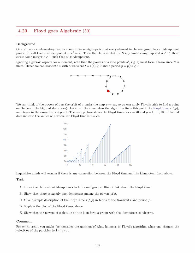
4.20. Floyd goes Algebraic (50)

BackgroundOne of the most elementary results about finite semigroups is that every element in the semigroup has an idempotentpower. Recall that x is idempotent if x2 = x. Then the claim is that for S any finite semigroup and a ∈ S, thereexists some integer r ≥ 1 such that ar is idempotent.Ignoring algebraic aspects for a moment, note that the powers of a (the points ai, i ≥ 1) must form a lasso since S isfinite. Hence we can associate a with a transient t = t(a) ≥ 0 and a period p = p(a) ≥ 1.

We can think of the powers of a as the orbit of a under the map x 7→ ax, so we can apply Floyd’s trick to find a pointon the loop (the big, red dot above). Let’s call the time when the algorithm finds this point the Floyd time τ(t, p),an integer in the range 0 to t+ p− 1. The next picture shows the Floyd times for t = 70 and p = 1, . . . , 100 . The reddots indicate the values of p where the Floyd time is t = 70.

Inquisitive minds will wonder if there is any connection between the Floyd time and the idempotent from above.

Task

A. Prove the claim about idempotents in finite semigroups. Hint: think about the Floyd time.

B. Show that there is exactly one idempotent among the powers of a.

C. Give a simple description of the Floyd time τ(t, p) in terms of the transient t and period p.

D. Explain the plot of the Floyd times above.

E. Show that the powers of a that lie on the loop form a group with the idempotent as identity.

CommentFor extra credit you might (re-)consider the question of what happens in Floyd’s algorithm when one changes thevelocities of the particles to 1 ≤ u < v.

185

4.21. Polynomial Equations Mod 2 (25)

BackgroundWe have seen that Diophantine equations are hard: it is undecidable whether a polynomial with integer coefficientshas an integer solution. By contrast, modular arithmetic is easy in the sense that one can conduct brute force searchover the finitely many possible values. Arithmetic over Zp, p a prime, is particularly interesting since we are dealingwith a field in this case.

Task

1. Show that any function f : Zn2 → Z2 can be expressed in terms of a polynomial P (x1, . . . , xn).

2. Show that one can solve a single polynomial equation P (x1, . . . , xn) = 0 over Z2 in polynomial time.

186

4.22. Functions versus Polynomials (30)

BackgroundFor a domain A with good algebraic properties, functions f : An → A can sometimes be described in terms ofpolynomials: find some multivariate polynomial P such that f = P . For clarity, we have written P for the functionAn → A induced by the polynomial P ∈ A[x1, . . . , xn] (one usually does not bother with this distinction and saysthings like “consider the function x 7→ x2 + 1”). In general there are not enough polynomials to describe all functions,but for arithmetic modulo a prime everything works out nicely.

Task

A. Let p be an arbitrary prime. Show that any function f : Znp → Zp can be expressed in terms of a polynomialP (x1, . . . , xn).

B. For p = 2, what does this have to do with Boolean functions?

C. How about functions f : Znm → Zm for a general modulus m? Say, m = 4?

D. Testing whether a single polynomial equation P (x1, . . . , xn) = 0 over the integers has a solution is undecidable.By contrast, show that over Z2 we can check in polynomial time whether there is a solution. Note: we are nottalking about systems of equations here, just a single one.

187

4.23. Functions versus Polynomials (30)

BackgroundFor a domain A with good algebraic properties, functions f : An → A can sometimes be described in terms ofpolynomials: find some multivariate polynomial P such that f = P . For clarity, we have written P for the functionAn → A induced by the polynomial P ∈ A[x1, . . . , xn] (one usually does not bother with this distinction and saysthings like “consider the function x 7→ x2 + 1”). In general there are not enough polynomials to describe all functions,but for arithmetic modulo a prime everything works out nicely.

Task

A. Let p be an arbitrary prime. Show that any function f : Znp → Zp can be expressed in terms of a polynomialP (x1, . . . , xn).

B. For p = 2, what does this have to do with Boolean functions?

C. How about functions f : Znm → Zm for a general modulus m? Say, m = 4?

D. Testing whether a single polynomial equation P (x1, . . . , xn) = 0 over the integers has a solution is undecidable.By contrast, show that over Z2 we can check in polynomial time whether there is a solution. Note: we are nottalking about systems of equations here, just a single one.

188

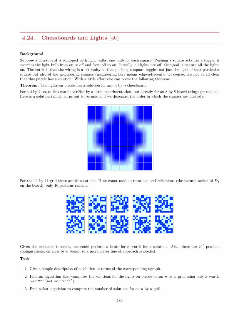
4.24. Chessboards and Lights (40)

BackgroundSuppose a chessboard is equipped with light bulbs, one bulb for each square. Pushing a square acts like a toggle, itswitches the light bulb from on to off and from off to on. Initially, all lights are off. Our goal is to turn all the lightson. The catch is that the wiring is a bit faulty so that pushing a square toggles not just the light of that particularsquare but also of the neighboring squares (neighboring here means edge-adjacent). Of course, it’s not at all clearthat this puzzle has a solution. With a little effort one can prove the following theorem:Theorem: The lights-on puzzle has a solution for any n by n chessboard.For a 4 by 4 board this can be verified by a little experimentation, but already for an 8 by 8 board things get tedious.Here is a solution (which turns out to be unique if we disregard the order in which the squares are pushed):

For the 11 by 11 grid there are 64 solutions. If we count modulo rotations and reflections (the natural action of D4on the board), only 10 patterns remain:

Given the existence theorem, one could perform a brute force search for a solution. Alas, there are 2n2 possibleconfigurations, on an n by n board, so a more clever line of approach is needed.

Task

1. Give a simple description of a solution in terms of the corresponding ugraph.

2. Find an algorithm that computes the solutions for the lights-on puzzle on an n by n grid using only a searchover 2n? (not over 2n×n?).

3. Find a fast algorithm to compute the number of solutions for an n by n grid.

189

4. Find a fast algorithm to compute an actual solution for an n by n grid.

CommentFast definitely means not exponential in n. Think vector spaces over the two-element field.Extra Credit 1: Find a solution for the 40 by 40 grid (plot a picture, it’s easy to check visually whether your solutionis correct using part (A)).

Extra Credit 2: Prove the existence theorem.

190

4.25. Shrinking Dimension (20)

BackgroundAs we have seen in class, there is a unique finite field F of size pk for any prime p and k ≥ 1. In one standardimplementation we then think of F as a vector space of dimension k over Fp, so the field elements are vectors ofmodular numbers. However, it is sometimes more convenient to deal with a lower-dimensional vector space over alarger ground field. More precisely, we may have a chain of subfields

Fp ⊆ K ⊆ F

and we can consider F as a vector space over K. Alas, this only works under special circumstances which will bedescribed in this problem.Fix some prime characteristic p throughout.

Task

A. Show that the following are equivalent, where 1 ≤ ` ≤ k:

(a) ` divides k(b) p` − 1 divides pk − 1(c) x` − 1 divides xk − 1 (in the polynomial ring Fp[x]).

B. Show that if K is a subfield of F then K is (isomorphic to) Fp` where ` divides k.

C. Show that if ` divides k then Fp` is (isomorphic to) a subfield of F.

CommentThe last item is the hardest; think splitting fields.

191

4.26. Building A Finite Field (20)

BackgroundAs we have seen in class, there is a unique finite field of size pk for any prime p and k ≥ 1. Needless to say, the casep = 2 it is particularly interesting for actual implementations: the prime field can naturally be represented by bitsand the arithmetic operations are given by xor (addition) and and (multiplication).Building a finite field F2k requires a little more work.

Task

A. Show how to construct the finite field F of size 256. What data structures would you use, how would youimplement arithmetic in this field.

B. How many primitive elements are there in this field?

C. What are all the subfields of F? Why?

D. If we had constructed a field of size 32, what would the subfields be?

E. What is the main difficulty in doing a similar construction for the field of size 21024?

192

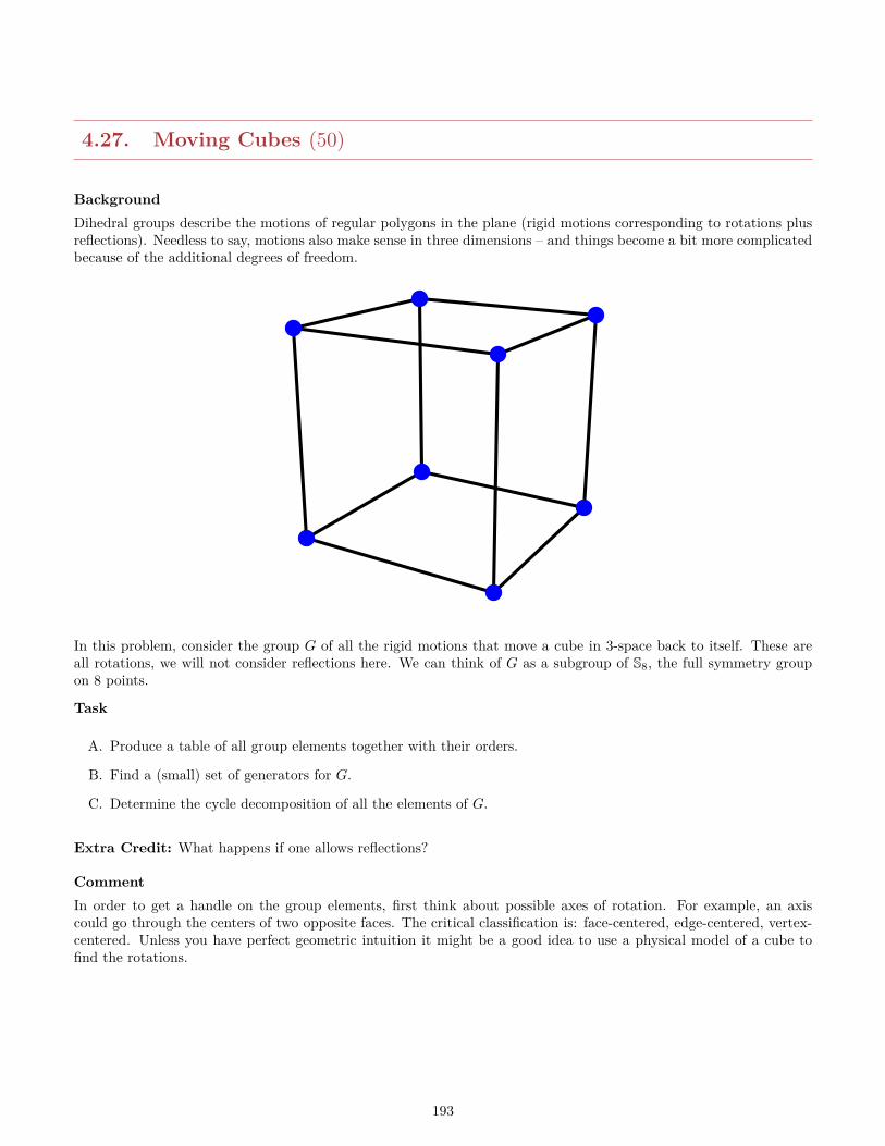
4.27. Moving Cubes (50)

BackgroundDihedral groups describe the motions of regular polygons in the plane (rigid motions corresponding to rotations plusreflections). Needless to say, motions also make sense in three dimensions – and things become a bit more complicatedbecause of the additional degrees of freedom.

In this problem, consider the group G of all the rigid motions that move a cube in 3-space back to itself. These areall rotations, we will not consider reflections here. We can think of G as a subgroup of S8, the full symmetry groupon 8 points.

Task

A. Produce a table of all group elements together with their orders.

B. Find a (small) set of generators for G.

C. Determine the cycle decomposition of all the elements of G.

Extra Credit: What happens if one allows reflections?

CommentIn order to get a handle on the group elements, first think about possible axes of rotation. For example, an axiscould go through the centers of two opposite faces. The critical classification is: face-centered, edge-centered, vertex-centered. Unless you have perfect geometric intuition it might be a good idea to use a physical model of a cube tofind the rotations.

193

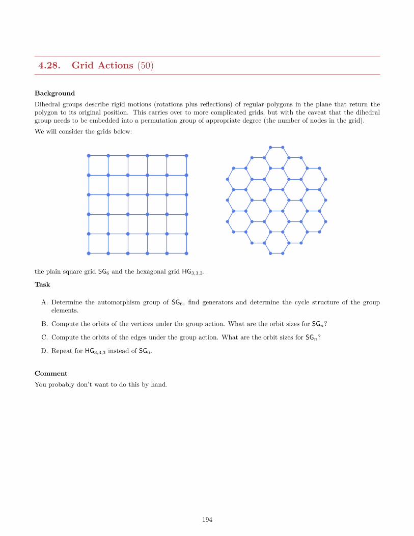
4.28. Grid Actions (50)

BackgroundDihedral groups describe rigid motions (rotations plus reflections) of regular polygons in the plane that return thepolygon to its original position. This carries over to more complicated grids, but with the caveat that the dihedralgroup needs to be embedded into a permutation group of appropriate degree (the number of nodes in the grid).We will consider the grids below:

the plain square grid SG6 and the hexagonal grid HG3,3,3.

Task

A. Determine the automorphism group of SG6, find generators and determine the cycle structure of the groupelements.

B. Compute the orbits of the vertices under the group action. What are the orbit sizes for SGn?

C. Compute the orbits of the edges under the group action. What are the orbit sizes for SGn?

D. Repeat for HG3,3,3 instead of SG6.

CommentYou probably don’t want to do this by hand.

194

4.29. Characteristic 2 (50)

BackgroundAs we have seen in class, there is a unique finite field of size pk for any prime p and k ≥ 1. When p = 2 it is particularlyeasy to give efficient implementations of the arithmetic in these fields.

Task

A. Explain how to implement the finite field F25 .

B. How difficult is it to implement addition and multiplication in your system? How about division?

C. How many primitive elements are there in F25?

D. What are all the subfields of F25? Why?

E. How does all of this carry over to F2k? What is the main difficulty in implementing the field of size 21000?

195

4.30. Redundant Field Representations (50)

BackgroundAs we have seen, it may be computationally advantageous to implement a finite field F2k by embedding it in a quotientring K = F2[x]/(xn+1) that fails to be a field itself. For example, F4 can be embedded into F2[x]/(x3 +1) (a generatorfor the multiplicative group is x+ 1).For this method to be of any practical use, the least n such that that F2[x]/(xn + 1) embeds F2k cannot be muchlarger than k. Let’s write η(k) for this “embedding number”. For example, it turns out that η(8) = 17. The followinglemma can be found in an otherwise excellent paper from 1998.

Lemma: η(k) = min(n > k | k = order of 2 in Zn?

)Recall that F2k is a subfield of F2` if, and only if, k divides `.

Task

A. Compute η(5) and η(10) according to this lemma.

B. Conclude that the lemma is false.

C. Fix the lemma.

196

Chapter 5

Combinatorics

197

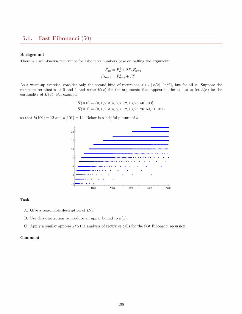
5.1. Fast Fibonacci (50)

BackgroundThere is a well-known recurrence for Fibonacci numbers base on halfing the argument:

F2n = F 2n + 2FnFn=1

F2n+1 = F 2n+2 + F 2

n

As a warm-up exercise, consider only the second kind of recursion: x 7→ bx/2c, dx/2e, but for all x. Suppose therecursion terminates at 0 and 1 and write H(x) for the arguments that appear in the call to x; let h(x) be thecardinality of H(x). For example,

H(100) = 0, 1, 2, 3, 4, 6, 7, 12, 13, 25, 50, 100H(101) = 0, 1, 2, 3, 4, 6, 7, 12, 13, 25, 26, 50, 51, 101

so that h(100) = 12 and h(101) = 14. Below is a helpful picture of h.

1000 2000 3000 4000 5000

12

14

16

18

20

22

24

Task

A. Give a reasonable description of H(x).

B. Use this description to produce an upper bound to h(x).

C. Apply a similar approach to the analysis of recursive calls for the fast Fibonacci recursion.

Comment

198

5.2. Pairing Sequences (50)

BackgroundA sequence S of positive integers is called a pairing sequence (of order n) if the length of S is 2n and each k ∈ [n]appears exactly twice in S; moreover, these two occurrences of k are separated by k other sequence elements.

Here are some examples of pairing sequences:3 2,3,1,2,1,34 2,3,4,2,1,3,1,47 4,5,6,7,1,4,1,5,3,6,2,7,3,28 4,5,6,7,8,4,1,5,1,6,3,7,2,8,3,211 6,7,8,9,10,11,5,6,1,7,1,8,5,9,4,10,3,11,2,4,3,212 6,7,8,9,10,11,12,6,5,7,1,8,1,9,5,10,4,11,3,12,2,4,3,215 8,9,10,11,12,13,14,15,7,8,1,9,1,10,5,11,7,12,6,13,5,14,4,15,3,6,2,4,3,216 8,9,10,11,12,13,14,15,16,8,7,9,1,10,1,11,5,12,7,13,6,14,5,15,4,16,3,6,2,4,3,2

As it turns out, there is a pairing sequence of order n iff n = −1, 0 (mod 4). The proof is a bit messy, so we won’t gothere.

Task

A. Stare hard at the previous examples and discover patterns of positions that can be easily precomputed. Forexample, the first entry is always dn/2e.

B. Implement an algorithm that will fill in the missing positions after precomputation. Explain how your algorithmworks and discuss it’s time complexity. What values of n can your algorithm handle (say, within 1 hour)?

CommentIn the examples above, my precomputation assigns positions for all but 1, 1, 2, 2, 3, 3, 3, 3 numbers k, respectively. Forn = 47 there are 10 missing numbers, and the second part of the algorithm fails at a time bound of 1000 seconds.

199

5.3. Self-Organizing Search (10)

BackgroundSuppose we are using a linked list to store distinct integers a1, a2, . . . , an. We will only deal with search operations:given an integer a (which appears on the list), traverse the list till a is found. Let us agree that the cost of such a searchoperation is the position i of a on the list, 1 ≤ i ≤ n. Now consider a sequence S of m such search operations; we areinterested in minimizing the total cost of S. Suppose that we are looking for ai a total of mi times (so

∑mi = m). If

we know these frequencies ahead of time, it is easy to organize a static list Lopt that minimizes the total cost of thesearch operations.Of course, in general we have no knowledge of the mi. Surprisingly, we can still perform searches within a bound oftwice the optimal cost if we use a simple adjustment: every time a is found in the list, it is moved to the front ofthe list (a simple constant time operation that we can ignore in cost). Let’s call this the self-organizing algorithm, asopposed to the unrealistic optimal list algorithm.Write CSO(S) for the cost of executing S in the self-organizing algorithm, and COL(S) for the corresponding cost inthe static algorithm. Note that COL = COL(S) does not depend on S (only on the mi), but CSO(S) can vary widelydepending on S.

Task

A. Explain how to construct the optimal static list Lopt and compute COL.

B. For L = (a, b) find a sequence S such that CSO(S) < COL and another sequence S′ such that CSO(S′) > COL;maximizing the difference in each case.

C. Find a bound for CSO(S) in terms of COL.Hint: first take a close look at your example in (B) to “guess” the right bound, then consider tri , the cost ofsearching for ai for the rth time.

D. Determine the relationship between the expected cost of a single search in the self-organizing algorithm and theexpected cost of a single search in the static algorithm.

200

5.4. Comparisons in Randomized Quicksort (10)

BackgroundWe have seen in class that a randomized version of quicksort (pivot is chosen at random from the given list) hasexpected running time O(n logn). Our argument was based on a brute force assault on the corresponding recurrenceequation. Here is a more elegant approach that focuses on the comparisons in quicksort.As always, assume we are sorting some permutation a = (a1, a2, . . . , an) of n distinct integers. Define C to be therandom variable: number of comparisons made during the execution of the algorithm on a.

Task

A. Write C as a sum of indicator variables.

B. Calculate the expected value of these indicator variables.

C. Use the result from (B) to determine E[C].

201

5.5. Shooting Blanks (10)

BackgroundHere is a simple problem dealing with matrices: suppose B is an n by n Boolean matrix; determine whether B has acolumn filled entirely with 0’s. We want a BCC algorithm (blank column checker) the solves this problem.For simplicity, let us describe running time only in terms of the number of lookups: the algorithm may query the bitat B[i, j], 1 ≤ i, j ≤ n which we count as one step. Of course, there is a trivial deterministic BCC that takes n2 stepsin the worst case. Moreover, given a particular choice of deterministic algorithm it is easy for an adversary to designa matrix B that forces the algorithm to spend n2 steps.There is an obvious lazy Las Vegas algorithm R:

• First permute the columns of B at random, say, C1, . . . , Cn.

• Then check the columns in this order, bailing out whenever a 1 is encountered.

As in class, let A be the class of all deterministic BCC algorithms and let I be the class of all inputs of size n by n;think of n as being fixed for simplicity. Recall Yao’s Minimax Principle:

minA∈A

E[TA(Iτ )] ≤ maxI∈I

E[TAσ (I)]

where the subscripts τ and σ indicate the probability distributions on I and A used to determine the expected values.

Task

A. Show that the expected number of queries of R is bounded by n(n+ 1)/2.

B. Give a reasonable description of A.

C. Show that for any Las Vegas algorithm A, the expected number of queries in the worst case is no better thann(n+ 1)/2. Hint: for reals α, β it suffices to show that (1− ε)α ≤ β for all ε > 0 in order to show that α ≤ β.

202

5.6. Vanilla Search Trees (10)

BackgroundThere are many clever techniques to balance search trees. In an effort to avoid implementation work, we can applythe “randomized incremental” paradigm to construct a reasonable search tree T from given, static data set A =a1, . . . , an, chosen from some ordered set.

Task

A. Describe a (the?) randomized incremental algorithm to construct a binary search tree.

B. Give a bound for the expected distance of a node in the tree from the root.

203

5.7. From Real to Binary (10)

BackgroundSuppose A is an n × n 0/1-matrix and x ∈ [0, 1]n a vector of reals in [0, 1]. We would like to replace x by a binary“approximation” x such that ‖A(x− x)‖∞ is minimal. Recall that the Chebyshev norm ‖z‖∞ of a vector z is themaximum of the absolute values of its components.One can show that this problem is NP-hard, so it is natural to look for a randomized algorithm:

1. Define indicator random variables Xi such that Pr[X = 1] = xi.

2. Set x = (X1, X2, . . . , Xn).

For simplicity write Z = A(x− x).

Task

A. Warmup: Let Ui, i = 1, . . . , n be independent random variables such that Pr[Ui = 1− pi] = pi and Pr[Ui = −pi] =1− pi, 0 ≤ pi ≤ 1. Set U =

∑Ui. Show that Pr[|U | ≥ a] ≤ 2e−2a2/n.

Hint: use piet(1−pi) + (1− pi)e−tpi ≤ et2/8.

B. Determine the expectation of Z1.

C. Bound the tail probability Pr[Z1 ≥ 2√n lnn].

D. Show that with probability O(1/n) we have ‖Z‖∞ <√n lnn.

204

5.8. Shifty Columns (10)

BackgroundSuppose A is an n by n binary matrix. Define the max-col-sum of A to be the maximum of all the column sums in A;in symbols mcs(A). For example, for

A =

1 1 1 0 1 01 0 0 0 0 11 0 0 0 1 11 0 0 0 1 01 0 0 1 1 11 0 0 0 0 0

we have mcs(A) = 6 because of the first column.Now suppose we can rotate the rows of the matrix, independently of each other. Clearly, any such operation can bedescribed by a shift vector s = (s1, s2, . . . , sn) where 0 ≤ si < n. Write A[s] for the matrix obtained by rotating therows according to shift vector s.Our goal is to find a shift vector s such that mcs(A[s]) is minimal; write mmcs(A) for the corresponding value. Forthe example above we can achieve the minimal value of 3 by rotating according to s = (0, 0, 0, 1, 4, 2) (altogether thereare 4416 shift vectors that work).Obviously, we do not wish to try out all nn shift vectors, so instead we use a randomized algorithm RandShift:

• Pick a shift vector s ∈ [0, n− 1] uniformly at random.

• Return A[s].

That’s it!

TaskLet A be an n by n binary matrix and C = mmcs(A) its min max col sum. Write R for the total number of 1’s in Aand call A sparse if R ≤ n lnn. Define X to be the random variable: sum of the first column in the matrix B producedby RandShift.

A. Show that the exptected value of X is optimal.

B. Assume that A is sparse. Use a Chernoff bound to show that mcs(B) ≥ C+4 lnn with probability at most 1/n2.

C. Assume that A is not sparse. Use a Chernoff bound to show that mcs(B) ≥ 5C with probability at most 1/n2.

In both cases the simplified bounds suffice.

205

5.9. Sparse Selection (10)

BackgroundSuppose A is a set of cardinality n, A ⊆ U for some totally ordered set U . Recall the clever randomized selectionalgorithm from class that computes ord(k,A) with probability 1 − O(n−1/4). As in class, we refuse to write ceilingsand floors.

1. Select a subset B ⊆ A of cardinality n3/4 at random (actually, sample with replacement).

2. Sort B.

3. Let κ = k/n1/4, κ− = max(κ−√n, 1), κ+ = min(κ+

√n, n3/4), b± = ord(κ±, B).

4. Compute r± = rk(b±, A) – note the A.

5. Let

A0 =

x ∈ A | x ≤ b+ if k < n1/4,x ∈ A | x ≥ b− if k > n− n1/4,x ∈ A | b− ≤ x ≤ b+ otherwise.

6. if t /∈ A0 or |A0| > 4n3/4 return to step 1.

7. Sort A0 and return ord(k − r− + 1, A0).

In class we gave part of the proof that with probability 1−O(n−1/4) the algorithm terminates after the first round: weshowed that ord(k,A) ∈ A0 with high probability. Here is the missing part of the proof: A0 has cardinality boundedby 4n3/4, with high probability. Again, for simplicity, we only consider the case x ∈ A | b− ≤ x ≤ b+ ; moreover,let’s just say k = n/2.Define the ranks λ− = max(n/2− 2n3/4, 1), λ+ = max(n/2 + n3/4, n) and the corresponding points a± = ord(λ±, A).

Task

A. Argue that it suffices to check that a− ≤ b− < b+ ≤ a+ (in fact, this condition is stronger than the cardinalitybound).

B. Using part (A), show that with probability 1−O(n−1/4) the cardinality bound holds for A0.

206

5.10. Plane Partitions (10)

BackgroundWe are given n non-overlapping line segments a1, . . . , an in the plane and we would like to partition the plane bystraight lines into convex regions in a way so that every region contains precisely one line segment. Alas, there isa glitch: to keep the computation simple we are not only allowed to use arbitrary auxiliary lines for the partition.Rather, we can only use (bi-infinite, one-way-infinite or finite) lines that are determined by the given line segmentsthemselves.To make this restriction feasible we have to relax the notion of “a region contains a line segment” a bit: we willonly insist that the line segments are not in the interior of the region, we are not concerned about the boundariesthemselves.Here is a simple randomized-incremental algorithm to determine such a partition.

1. Randomly permute the line segments, yielding a list a1, . . . , an. Initialize the partition to P to contain thesingle region R2.

2. While the partition is not finished, do the following: pick the first ai on the list that can be used to split one ofthe regions in P whose interior currently contains (part of) a line segment. Extend ai in the right way in bothdirections to split the region.

The example below makes the algorithm clear. We are interested in the random variable X, the number of regions inP produced by the algorithm. Note that every line segment will be used at some point, but since the auxiliary linesmay intersect line segments there may be more than n+1 regions. In fact, there could be as many as O(n2). However,our randomized approach makes this unlikely, we can expect to get only O(n logn) regions.To avoid pesky special cases, assume the given segments are not collinear.Given a line segment u, one of the auxiliary lines through u = u0 may cut through line segments u1, u2, . . . , us untilit either runs off to infinity or ends at some other boundary line already constructed. Define the predicate cut(u, v) ifan auxiliary line through u cuts through v. Define a kind of “distance” between u and v based on the partition:

dist(u, v) =i if v = ui is ith line on an auxiliary line through u,∞ otherwise.

Note that there could be two line segments v and v′ such that dist(u, v) = dist(u, v′). There are 8 regions in thefinished partition.

207

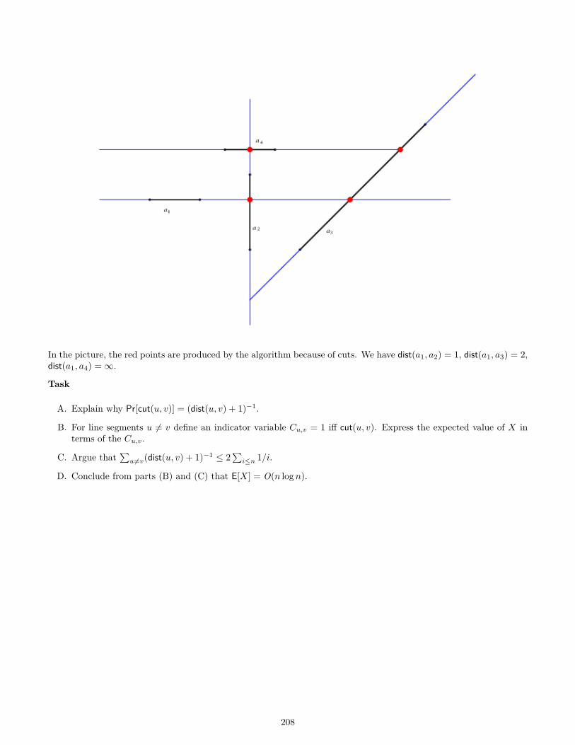
In the picture, the red points are produced by the algorithm because of cuts. We have dist(a1, a2) = 1, dist(a1, a3) = 2,dist(a1, a4) =∞.

Task

A. Explain why Pr[cut(u, v)] = (dist(u, v) + 1)−1.

B. For line segments u 6= v define an indicator variable Cu,v = 1 iff cut(u, v). Express the expected value of X interms of the Cu,v.

C. Argue that∑u 6=v(dist(u, v) + 1)−1 ≤ 2

∑i≤n 1/i.

D. Conclude from parts (B) and (C) that E[X] = O(n logn).

208

5.11. Max-of-Two Quicksort (10)

BackgroundWe have seen that random pivot selection in quicksort results in expected running time of O(n logn). In reality, it isoften preferable to choose the pivot deterministically, typically by sampling in a few places and then using the medianor some such. Here is a very simple method: use the maximum of a1 and a2 as pivot.As always, assume that all elements in the given list A are distinct and that A has length n.Write X for the random variable: length of the left sublist after partitioning.

Task

A. What is the possible range of X?

B. What is Pr[X = k] for k in this range?

C. What is E[X]?

209

5.12. The Best of Times, the Worst of Times (50)

Background

BackgroundGiven a permutation π of [n] = 1, 2, . . . , n, we want to compute the position of 1 in π. There is an obviousdeterministic algorithm LtR: start at π1 and go right until 1 is found. A randomized version RLR of the algorithmfirst flips a fair coin and then either searches left-to-right (i.e., it runs LtR) or it searches right-to-left, starting at πn.Let P be the set of all permutations of [n]. TA(π) denotes the running time on algorithm A on input π and we thinkof TA(π) as a random variable (albeit a boring one if A is deterministic).Define the best/worst/average average-case running time of A as follows:

T bA(n) = min( E[TA(π)]

∣∣ π ∈ P )TwA (n) = max( E[TA(π)]

∣∣ π ∈ P )

T aA(n) = 1/n!

∑π

E[TA(π)]

Task

A. Determine the following values precisely.

T bLtR(n) =

TwLtR(n) =

T aLtR(n) =

B. Determine the following values precisely.

T bRLR(n) =

TwRLR(n) =

T aRLR(n) =

C. How about quicksort where the pivot is the first element in the array? Asymptotic answers are good enough.

T bQS1(n) =

TwQS1(n) =

T aQS1(n) =

D. How about quicksort with randomized pivot selection? Asymptotic answers are good enough.

210

T bRQS(n) =

TwRQS(n) =

T aRQS(n) =

211

5.13. MinMax Trees (100)

BackgroundRecall from lecture the circuits defined by

T1(x1, x2, x3, x4) = (x1 ∨ x2) ∧ (x3 ∨ x4)

Tk+1(x1,x2,x3,x4) = T1 (Tk(x1), Tk(x2), Tk(x3), Tk(x4))

Our goal is to evaluate the circuit Tk reading as few bits of the given truth assignment α : 24k → 2 as possible. Weread the bits left-to-right.

Task

A. Prove that T1 increases the bias for p ≥ (3−√

5)/2 ≈ 0.38.

B. Prove that E[Sk] = 3k = nlog4 3 ≈ n0.79

212

5.14. Lots of Stars (30)

BackgroundConsider the following languages over the alphabets a, b and a, b, c, respectively.

L1 = (b∗a)i(a∗b)i | i ≥ 1

L2 = (ab∗)i(a∗b)i | i ≥ 1

L2 = (ab∗)ic(a∗b)i | i ≥ 1

Task

A. Determine whether L1 is regular. If it turns out that the language fails to be regular, check whether it iscontext-free.

B. Repeat for L2.

C. Repeat for L3.

213

5.15. Deterministic Counting (20)

BackgroundLet’s return to the counting language K = x ∈ a, b? | #ax = #bx . It is not hard to see that K is context-free,but one can push a bit further.For this problem, we assume that a deterministic PDA accepts by final state only (disregarding the stack contents).

Task

A. Construct an unambiguous CFG for K.

B. Construct a deterministic PDA for K.

214

5.16. Typical Context-Free Languages (30)

BackgroundChecking whether a language is regular is usually quite straightforward. By contrast, checking whether a givenlanguage is context-free can be a little tricky. Quite tricky, in fact.

Task

A. Construct a CFG for the counting language K = x ∈ a, b? | #ax = #bx and prove that your grammar iscorrect.

B. Construct a CFG for the “marked unequal language” U = xcy | x, y ∈ a, b? ∧ x 6= y and prove that yourgrammar is correct.

C. Show that the copy language C = xx | x ∈ a, b? is not context-free.

CommentIt is critical that you explain the purpose of your productions, it is very hard to decipher an uncommented CFG.

215

5.17. Linear Grammars (20)

BackgroundA context-free grammar is right linear if all its productions are of the form A xB or A x where A,B ∈ V , x ∈ Σ?.The grammar is left linear if all its productions are of the form A Bx or A x.

Task

A. Show that every right linear grammar generates a regular language.

B. Show that every regular language can be generated by a right linear grammar.

C. Repeat for left linear instead of right linear.

D. What would happen if we allowed both left linear and right linear productions in the same grammar?

CommentFor part (C), make sure to come up with an elegant, short argument.

216

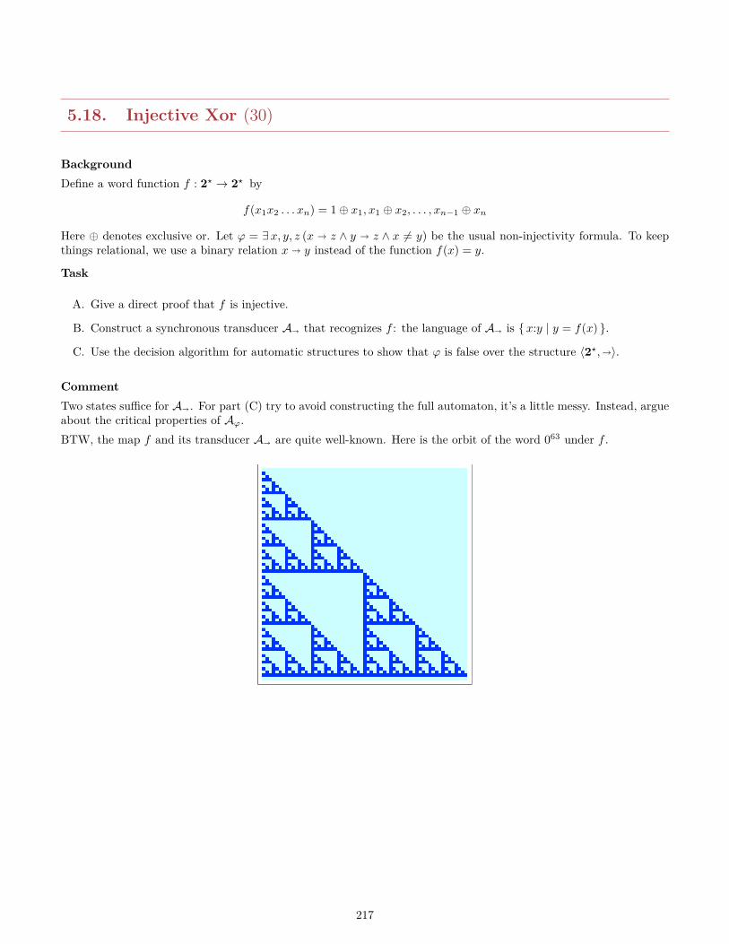
5.18. Injective Xor (30)

BackgroundDefine a word function f : 2? → 2? by

f(x1x2 . . . xn) = 1⊕ x1, x1 ⊕ x2, . . . , xn−1 ⊕ xn

Here ⊕ denotes exclusive or. Let ϕ = ∃x, y, z (x z ∧ y z ∧ x 6= y) be the usual non-injectivity formula. To keepthings relational, we use a binary relation x y instead of the function f(x) = y.

Task

A. Give a direct proof that f is injective.

B. Construct a synchronous transducer A that recognizes f : the language of A is x:y | y = f(x) .

C. Use the decision algorithm for automatic structures to show that ϕ is false over the structure 〈2?,〉.

CommentTwo states suffice for A. For part (C) try to avoid constructing the full automaton, it’s a little messy. Instead, argueabout the critical properties of Aϕ.BTW, the map f and its transducer A are quite well-known. Here is the orbit of the word 063 under f .

217

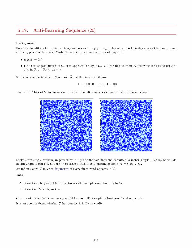
5.19. Anti-Learning Sequence (20)

BackgroundHere is a definition of an infinite binary sequence U = u1u2 . . . un . . . based on the following simple idea: next time,do the opposite of last time. Write Un = u1u2 . . . un for the prefix of length n.

• u1u2u3 = 010

• Find the longest suffix v of Un that appears already in Un−1. Let b be the bit in Un following the last occurrenceof v in Un−1. Set un+1 = b.

So the general pattern is . . . avb . . . av∣∣ b and the first few bits are

0 1 0 0 1 1 0 1 0 1 1 1 0 0 0 1 0 0 0 0

The first 212 bits of U , in row-major order, on the left, versus a random matrix of the same size:

Looks surprisingly random, in particular in light of the fact that the definition is rather simple. Let Bk be the deBruijn graph of order k, and use U to trace a path in Bk, starting at node Uk = u1u2 . . . uk.An infinite word V in 2ω is disjunctive if every finite word appears in V .

Task

A. Show that the path of U in Bk starts with a simple cycle from Uk to Uk.

B. Show that U is disjunctive.

Comment Part (A) is eminently useful for part (B), though a direct proof is also possible.It is an open problem whether U has density 1/2. Extra credit.

218

5.20. h-Sorting (50)

BackgroundA list x = (x1, . . . , xn) is h-sorted if xi ≤ xi+h, so 1-sorted is the same as sorted. An h-sorting algorithm establishesh-sortedness (and is thus potentially weaker that a full sorting algorithm). This is exploited in the shellsort algorithm.Let x = (x1, . . . , xn) and y = (y1, . . . , yn) be two lists of length n such that xi ≤ yi and denote their sorted versionsby x′ and y′.

Task

A. Show that x′i ≤ y′i.

B. Show that h-sorting does not affect a k-sorted file, for all h and k.

Comment

219

5.21. Monotone Boolean Functions (50)

BackgroundConsider Boolean functions on n variables, f : 2n → 2 . Order bit-vectors by the standard product order: x ≤ yiff xi ≤ yi for all i ∈ [n]. A Boolean function is monotone if x ≤ y implies f(x) ≤ f(y). It is easy to see that thenumber of n-ary Boolean functions is 22n , but counting the number of monotone Boolean functions is much harder.The number of n-ary monotone Boolean functions is called the nth Dedekind number, written Dn. Here are the firstfew Dedekind numbers:

n 0 1 2 3 4 5 6Dn 2 3 6 20 168 7581 7828354

Let us say that two nary Boolean functions f and g are equivalent if one can be obtained from the other by permutingvariables:

f(x1, x2, . . . , xk) = g(xπ(1), xπ(2), . . . , xπ(k))

where π is some permutation of [n]. We write dn for the number of equivalence classes. For example, d2 = 5:

0, 1, x, x+ y, xy

Task

A. Show that a Boolean function is monotone iff it can be written in terms of ∧ and ∨.

B. Calculate d3.

Comment D6 was only computed as recently as 1946; today, D8 and d7 are known.

220

5.22. Circle Divisions (50)

BackgroundConsider a circle and pick n distinct points on its perimeter. Then draw all possible chords between these points toobtain a subdivision. Assume that no three lines intersect in one point in the interior of this subdivision. Write Cnfor the number of regions.

Task

A. Argue that Cn is well-defined.

B. Calculate the value for Cn for n ≤ 5.

C. The last part suggests a simple closed form for Cn. Which one?

D. Argue that the apparent closed form is quite wrong as follows: consider a disk of radius one meter and , say,n = 30. Think of having 30 pegs connected by very thin thread.

E. Hard: Come up with closed form for Cn.

Comment

221

5.23. Binomial Sums (50)

Background

We already know that∑ni=0(ni

)= 2n and

∑n/2i=0(n2i)

= 2n−1. How about

n/3∑i=0

(n

3i

)

TaskProduce a closed form for this sum.

Comment Make sure to come up with an elegant argument, not some brute-force slog through tedious details.

222

5.24. Fibonacci Identities (50)

Background

Task

A. Show thatn∑i=0

(r + i

i

)=(n+ r + 1r + 1

)B. Show that

n/2∑i=0

(n− ii

)= Fn+1

223

5.25. List Operations (50)

BackgroundFor this problem we think of lists as being inductively defined like so.

nil the empty lista :: L the list with first element a and tail L

Here a is chosen from some groundset that is of no concern to us. So, the only basic operation is prepend: a :: Leffectively prepends a to L. The list is usually written in more casual form as (a, b, c) would be represented bya :: b :: c :: nil (we assume :: associates to the right).We can define a number of operations on these lists by induction.Append

app(nil, a) = a :: nilapp(b :: L, a) = b :: app(L, a)

Join

join(nil, B) = B

app(a :: A,B) = a :: join(A,B)

Reverse

rev(nil) = nilrev(a :: A) = app(rev(A), a)

Length

len(nil) = 0len(a :: A) = len(A) + 1

Search

search(nil, a) = 0search(b :: A, a) = (a = b) ∨ search(A, a)

Task

A. Establish the following identities:

rev(app(A, a)) = a :: rev(A)rev(rev(A)) = A

rev(join(A,B)) = join(rev(B), rev(A))

B. Establish the following identities:

len(rev(A)) = len(A)len(join(A,B)) = len(A) + len(B)

C. Establish the following identities:

search(app(A, b), a) = (a = b) ∨ search(A, a)search(rev(A), a) = search(A, a)

search(join(A,B), a) = search(A, a) ∨ search(B, a)

224

5.26. List Multiplication (50)

BackgroundIn this problem all lists are binary and non-empty. We write AB for the join of lists A and B; Aa indicates that thelast element is a. Here is a kind of list multiplication:

A⊗ 0 = A,A⊗ 1 = A

A⊗Bb = (A⊗B)(A⊗ b)

For example, 01⊗ 001 = 010110. Clearly |A⊗B| = |A||B|.One interesting application of this multiplication is the definition of infinite sequences. Suppose we have a seed list Aand a sequence of lists (Bn). Define

Cn = A⊗ 0B1 ⊗ 0B2 ⊗ . . .⊗ 0BnNote that Cn is a proper prefix of Cn+1 (we multiply by 0Bn+1), so we can define the limit C = limCn. The pointhere is that even though A and Bn may be very simple, the resulting sequence C may have interesting properties.

Task

A. Show the following identities involving list multiplication.

A⊗ (BC) = (A⊗B)(A⊗ C)A⊗B = A⊗B = A⊗ C

A⊗ (B ⊗ C) = (A⊗B)⊗ C

B. Conclude that non-empty binary lists together with multiplication and 0 form a monoid. Is this monoid com-mutative?

C. Show that the sequence defined by0⊗ 01⊗ 01⊗ 01⊗ . . .

is the Morse-Thue sequence.

D. Show that the sequence defined by A and (Bn) is periodic if, and only if, one of the following two conditionsholds: for all sufficiently large n, 0Bn = 00 . . . 00, or for all sufficiently large n, 0Bn = 0101 . . . 10.

225

5.27. Double Permutations (50)

BackgroundConsider permutations over the multiset Σ = a1, a1, . . . , an, an.Call such a permutation clean if there is no block aiai in the permutation, for any i.

Task

A. Give a closed form for the number of all permutations over Σ.

B. Determine all clean permutations when n = 3.

C. Find a reasonable representation for the number of clean permutations.

D. How many clean permutations are there for n = 10?

Comment

226

5.28. Fashion Show (50)

BackgroundFor a fashion show there are n skirts in the n most fashionable colors, and n blouses, also in these colors. They needto be paired up.

Task

A. An assistant is asked to combine skirts with blouses, avoiding pairs of the same color. How many arrangementsare there?

B. The next day, the assistant is still slightly drunk from the party the night before and only manages to avoidmatching items of the same color (but may combine a skirt with another). How many possible drunk arrange-ments are there?

Comment

227

5.29. Chameleons (50)

BackgroundOn a certain tropical island, there are three populations of chameleons: red, green, and blue. If two chameleons withdistinct colors meet, they both change color to the third color. So, a red and a green would produce two blue.Starting at 12 red, 13 green and 14 blue chameleons, can one reach a homogeneous population?

Task

A. Model the problem in terms of graphs and compute an answer using standard graph algorithms.

B. Take a close look at the results from part (A) and give a direct explanation that does not rely on computation.

Comment

228

5.30. Chainless Maps (50)

BackgroundLet P be the collection of all non-empty subsets of [n]. A map f : P → [n] is chainless if f−1(k) is an anti-chain inP , for all k in the image of f .

Task

A. Show that f(X) = |X| is chainless.

B. Let π be a permutation of [n]. Show that f(X) = π(|X|) is chainless.

C. Characterize all chainless maps.

Comment

229

5.31. Chains (50)

BackgroundConsider a list L = (a1, a2, . . . , am) of m distinct elements of some total order 〈A,<〉. A ascending/descending chainin L is a sublist whose elements are strictly increasing/decreasing.

Task

A. Show that for n = m2 + 1, every list L of length n has a chain of length m+ 1. Hint: consider maximal chainsending at ak.

B. Show that the last result cannot be improved to hold for n = m2.

C. Show that both 〈A,<〉 and 〈A,>〉 are well-orders iff A is finite.

Comment

230

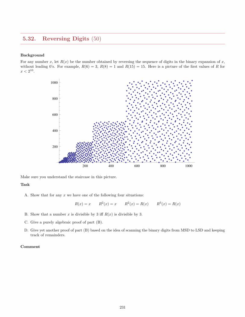
5.32. Reversing Digits (50)

BackgroundFor any number x, let R(x) be the number obtained by reversing the sequence of digits in the binary expansion of x,without leading 0’s. For example, R(6) = 3, R(8) = 1 and R(15) = 15. Here is a picture of the first values of R forx < 210.

200 400 600 800 1000

200

400

600

800

1000

Make sure you understand the staircase in this picture.

Task

A. Show that for any x we have one of the following four situations:

R(x) = x R2(x) = x R2(x) = R(x) R3(x) = R(x)

B. Show that a number x is divisible by 3 iff R(x) is divisible by 3.

C. Give a purely algebraic proof of part (B).

D. Give yet another proof of part (B) based on the idea of scanning the binary digits from MSD to LSD and keepingtrack of remainders.

Comment

231

5.33. EAN (50)

BackgroundMany commercial items such as books, dog food, hair spray, and so on, are identified by a codenumbers. A well-knownexample is the ISBN (international standard book number). ZIP codes are an example for codenumbers attachedto postal districts. Since these numbers are often copied it is important to build in some mechanism that makes itfeasible to discover errors. To this end, codenumbers often incorporate a special digit, the check digit, whose purposeit is to provide additional information that allows one to verify that the other digits are all correct, at least in somecases.Here is a concrete example: EANs (European Article Numbers). An EAN consists of 13 decimal digits:

x1x2x3 . . . x12x13

The first two code the country, the next five the manufacturer, and the next five the actual article. The last digit isthe check digit. For example,5000127016996 Kellog’s Corn Flakes8001060375109 Scala Pesto SauceThe rule which determines the last digit is that

(x1 + x3 + x5 . . .+ x11) + 3(x2 + x4 + x6 . . .+ x12) + x13

is divisible by 10.

Task

A. Show that a single digit error can be detected by the EAN system.

B. The purpose of splitting the sum is to make transpositions (switching two adjacent digits, something that happensoften in typing) detectable. Show that EANs detect some, but not all transpositions. Explain exactly whichtranspositions go undetected.

C. Repeat parts (A) and (B) for a modified scheme where the multiplier 3 is replaced by 5. How about a multiplierof 2?

D. Based on part (C), why was 3 chosen as the multiplier?

Comment

232

5.34. Surjectivity (50)

BackgroundRecall the notation for composition: relational composition is ρ • σ but functional composition is f g (and goes inthe opposite direction). So ρ : A→ B and σ : B → C but for the functions f : B → C and g : A→ B.You might find it expedient on occasion to write xfy rather than f(x) = y.

TaskShow that the following are equivalent.

A. Function f : A −→ B is surjective.

B. IB ⊆ f c • f .

C. ∃ F : B −→ A (f F = IB).

D. ∀ g, h : B −→ C (g f = h f =⇒ g = h).

Comment

233

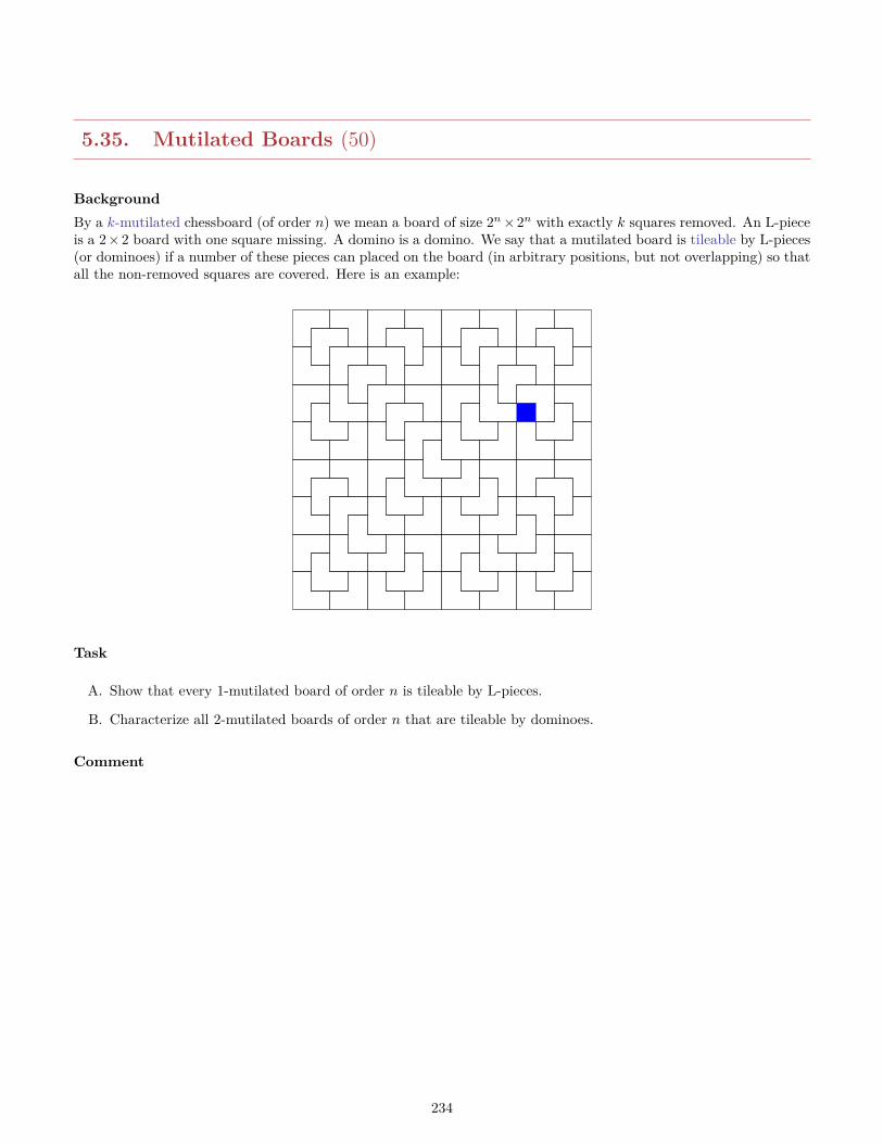
5.35. Mutilated Boards (50)

BackgroundBy a k-mutilated chessboard (of order n) we mean a board of size 2n×2n with exactly k squares removed. An L-pieceis a 2×2 board with one square missing. A domino is a domino. We say that a mutilated board is tileable by L-pieces(or dominoes) if a number of these pieces can placed on the board (in arbitrary positions, but not overlapping) so thatall the non-removed squares are covered. Here is an example:

Task

A. Show that every 1-mutilated board of order n is tileable by L-pieces.

B. Characterize all 2-mutilated boards of order n that are tileable by dominoes.

Comment

234

5.36. Generalized Checkerboards (50)

BackgroundConsider a n × n grid whose nodes are colored red or blue. A coloring is admissible when all 2 × 2 subsquares haveexactly two red and two blue squares. For example, an ordinary checkerboard is admissible.

Task

A. Count the number of admissible n× n boards.

B. When is the probability that a randomly chosen board is admissible less than 10−3?

235

5.37. Flattening Multisets (50)

BackgroundA finite multiset over a set A can be thought of as a map α : A→ N such that α(a) > 0 for only finitely many a ∈ A.Intuitively, α(a) is the multiplicity of object a in α. The weight of α is

∑α(a). Call a multiset flat if it represents a

plain set: α(a) ≤ 1 for all a.We are here interested in finite multisets over the natural numbers. Let’s consider two operations on these multisets,shift and cancel. The shift operation transforms α into β provided that for some k, α(k) ≥ 2 and β agrees with αexcept that β(k) = α(k) − 2, β(k + 2) = α(k + 2) + 1, β(k + 3) = α(k + 3) + 1. For cancel we have for some k,α(k) ≥ 2, α(k + 1) ≥ 2 and α(k + 2) ≥ 1; β agrees with α except that β(k) = α(k)− 2, β(k + 1) = α(k + 1)− 2 andβ(k + 2) = α(k + 2)− 1.We say that α reduces to β if there is a sequence of shift and cancel operations that leads from α to β. For example,

(3, 2, 0, 0, 0, 0, 0, 0, . . .) shift−→

(1, 2, 1, 1, 0, 0, 0, 0, . . .) shift−→

(1, 0, 1, 2, 1, 0, 0, 0, . . .) shift−→(1, 0, 1, 0, 1, 1, 1, 0, . . .)

and

(3, 0, 1, 1, 1, 0, 0, 0, . . .) shift−→

(1, 0, 2, 2, 1, 0, 0, 0, . . .) shift−→

(1, 0, 0, 2, 2, 1, 0, 0, . . .) cancel−→(1, 0, 0, 0, 0, 0, 0, 0, . . .)

We will establish the following

Claim 1: Every finite multiset of natural numbers reduces to a flat multiset under the operations of shift and cancel.

The following function will be useful in the proof of Claim 1. Let f : N3 → N3 be defined by f(x, y, z) = (y, z+x/2, x/2)where x/2 denotes integer division.

Claim 2: The map f is 2-to-1 and all orbits of f end in fixed points of the form (2i, 2i, i).

For example, the following orbit of f ends in (2, 2, 1).

(2, 3, 4), (3, 5, 1), (5, 2, 1), (2, 3, 2), (3, 3, 1), (3, 2, 1), (2, 2, 1)

Task

A. Show that the shift operations alone is not enough to reduce an arbitrary finite multiset to a flat multiset.

B. Show that Claim 1 follows from Claim 2.

C. Write fn(x, y, z) as three rational polynomials in x, y, z and find a recurrence equation for the coefficients ofthese polynomials. Hint: compute a few values and find a pattern.

D. Using this characterization of the polynomials prove Claim 2. Hint: assume fn(x, y, z) = (x, y, z) for some n > 0.

Comment Appearances notwithstanding, this problem is not artificial but arises naturally in a proof that showsthat a certain monoid of functions is isomorphic to the commutative free group on two generators.

236

5.38. Pruning Labels (50)

BackgroundIn an ordered tree T any two nodes x and y must have a uniquely determined lowest common ancestor (LCA): thelowest node in T that has both nodes as descendants. Thus, the LCA is the node z such that the subtree T (z) containsboth x and y but this property fails for all the children z′ of z. A node x is said to be to the left of y if they do notlie on the same branch and, letting z be the LCA with children z1, . . . , zk we have x ∈ T (zi) and y ∈ T (zj) for somei < j.Here is a problem that occurs in an important algorithm in automata theory. Consider finite ordered trees whosenodes are labeled by subsets of some finite set Q; we write λ(x) for the label of x. We need to remove all elementsfrom λ(y) that also occur in some label λ(x) where x is to the left of y. We will call this process horizontal pruning.Also, we would like to remove the labels of all descendants of y and refer to this as vertical pruning.

Task

A. Find an algorithm to do horizontal pruning that runs in time linear in the number of tree nodes, assuming thatthe set operations are constant time.

B. Find an algorithm to do vertical pruning that runs in time linear in the number of tree nodes, assuming thatthe set operations are constant time.

C. Find a way to combine your two algorithms into one (of course, that does not mean to compose them sequentially).

CommentMake sure to prove that your algorithms are correct.

237

5.39. Power Sums (50)

BackgroundLet us write

P (n, k) =n∑i=1

ik

for power sums. It is not hard to see that P (n, k) is a polynomial of degree k + 1 in n, but finding the coefficients isa bit more problematic. Here is a elegant but somewhat mysterious approach. Let’s suppose that

(S − 1)n = Sn

Don’t worry, keep reading. We now can write

(k + 1)ik = (i+ S)k+1 − (i− (S − 1))k+1

Rewrite P (n, k) as a telescoping sum and get

P (n, k) = (n+ S)k+1 − Sk+1

k + 1

A nice closed from except for the little problem with S.

Task

A. Show that P (n, k) is a polynomial of degree k + 1 in n.

B. Explain how to interpret Si as an unknown Si and exploit this interpretation to compute the polynomial forP (n, 10).

CommentThis involves solving a few linear equations, you probably do not want to do this by hand.

238

5.40. 3,5,7-Ordered Sequences (50)

BackgroundLet A be any sequence of distinct integers of length n. A is h-ordered if Ai < Ai+h for all i ≤ n−h. So any 1-orderedsequence is also sorted. There is a famous sorting algorithm due to D. L. Shell in 1959 that sort as list by performingrepeated insertion sorts on sublist of different strides. For example, a variant suggested by Knuth would sort a list oflength 10000 by making it h-sorted for h = 9841, 3280, 1093, 364, 121, 40, 13, 3, 1. Incidentally, the analysis of Shell-sortis excruciatingly difficult.This is the type of question that can be solved by some informed trial-and-error. What we are after here, though, isa more systematic attack. To this end, we consider the local order structure of a sequence. Consider the blocks ofwidth 5 of the sequence, and replace them by their order type. E.g., the sequence

50, 52, 56, 75, 55, 18, 77, 15

produces(1, 2, 4, 5, 3), (2, 4, 5, 3, 1), (3, 4, 2, 1, 5), (4, 3, 2, 5, 1)

Note that there are restrictions on how these blocks can follow one another.

Task

A. Analyze the local order structure of 3,5-ordered sequences.

B. Use your results to construct a 3,5,7-ordered sequence of length 106 that has more than 106 inversions.

Comment

239

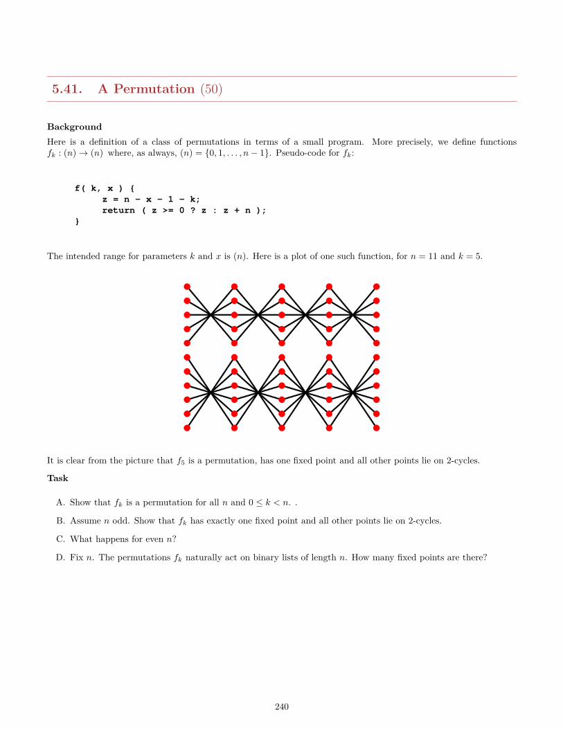
5.41. A Permutation (50)

BackgroundHere is a definition of a class of permutations in terms of a small program. More precisely, we define functionsfk : (n)→ (n) where, as always, (n) = 0, 1, . . . , n− 1. Pseudo-code for fk:

f( k, x ) z = n - x - 1 - k;return ( z >= 0 ? z : z + n );

The intended range for parameters k and x is (n). Here is a plot of one such function, for n = 11 and k = 5.

It is clear from the picture that f5 is a permutation, has one fixed point and all other points lie on 2-cycles.

Task

A. Show that fk is a permutation for all n and 0 ≤ k < n. .

B. Assume n odd. Show that fk has exactly one fixed point and all other points lie on 2-cycles.

C. What happens for even n?

D. Fix n. The permutations fk naturally act on binary lists of length n. How many fixed points are there?

240

5.42. Kraft’s Inequality (50)

BackgroundKraft’s inequality is a combinatorial lemma that is often used in the theory of prefix codes; it is also crucial for theconstruction of Chaitin’s Ω.

Kraft’s Lemma:Let S ⊆ 2? be a prefix set of binary words. Then ∑

x∈S2−|x| ≤ 1

On the other hand, given natural numbers `n such that∑n≥1

2−`n ≤ 1

there exists a prefix set S = sn | n ⊆ 2? such that `n = |sn|. S is said to realize (`n). For example, `n = n produces∑2−`n = 1 and can be realized by sn = 0n−11.

Task

A. Prove the first part for any finite set S.

B. Prove the second part for any finite set S.

C. Conclude that the lemma holds for arbitrary sets.

CommentTry to be as algorithmic in the second part as possible. For the sake of TA sanity, let’s all assume that (`n) is anordered sequence.What exactly is needed to make the transition to the infinite case?

241

5.43. Non-Decreasing Functions (50)

TaskIn class we showed how to rank and unrank injective functions as well as strictly increasing functions f : [m] → [n] .This problem deals with slightly different class: non-decreasing functions (so f(i) ≤ f(i+ 1)).

Task

A. How many non-decreasing functions are there in terms of m and n?

B. Describe a good ranking and unranking function for the class of non-decreasing functions.

C. What are the time complexities of your rank and unrank operations?

CommentTry to come up with an elegant solution, it should easy to describe what you are doing. If you are using a complicatedmethod make sure to prove that it is correct.

242

5.44. Tic-Tac-Toe (20)

TaskUse the material in class to give a complete solution for the odious Tic-Tac-Toe problem. Let G ⊆ S9 be the requiredgroup acting on the board.

1. Determine the cycle structure of all the elements of G.

2. Determine the number of patterns with 3 naughts and 3 crosses.

3. Determine the complete pattern inventory.

243

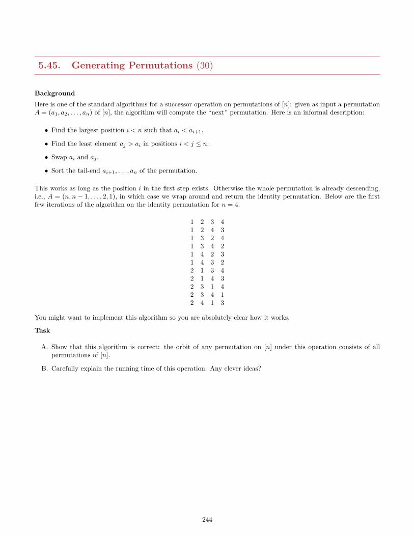
5.45. Generating Permutations (30)

BackgroundHere is one of the standard algorithms for a successor operation on permutations of [n]: given as input a permutationA = (a1, a2, . . . , an) of [n], the algorithm will compute the “next” permutation. Here is an informal description:

• Find the largest position i < n such that ai < ai+1.

• Find the least element aj > ai in positions i < j ≤ n.

• Swap ai and aj .

• Sort the tail-end ai+1, . . . , an of the permutation.

This works as long as the position i in the first step exists. Otherwise the whole permutation is already descending,i.e., A = (n, n − 1, . . . , 2, 1), in which case we wrap around and return the identity permutation. Below are the firstfew iterations of the algorithm on the identity permutation for n = 4.

1 2 3 41 2 4 31 3 2 41 3 4 21 4 2 31 4 3 22 1 3 42 1 4 32 3 1 42 3 4 12 4 1 3

You might want to implement this algorithm so you are absolutely clear how it works.

Task

A. Show that this algorithm is correct: the orbit of any permutation on [n] under this operation consists of allpermutations of [n].

B. Carefully explain the running time of this operation. Any clever ideas?

244

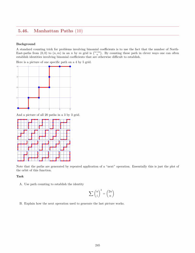
5.46. Manhattan Paths (10)

BackgroundA standard counting trick for problems involving binomial coefficients is to use the fact that the number of North-East-paths from (0, 0) to (n,m) in an n by m grid is

(n+mn

). By counting these path in clever ways one can often

establish identities involving binomial coefficients that are otherwise difficult to establish.Here is a picture of one specific path on a 4 by 5 grid.

1 2 3 4 5

1

2

3

4

And a picture of all 20 paths in a 3 by 3 grid.

Note that the paths are generated by repeated application of a “next” operation. Essentially this is just the plot ofthe orbit of this function.

Task

A. Use path counting to establish the identity

∑(n

i

)2=(

2nn

)B. Explain how the next operation used to generate the last picture works.

245

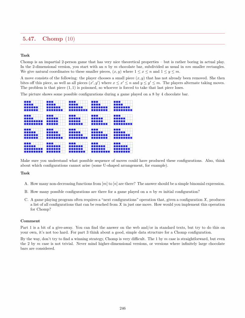
5.47. Chomp (10)

TaskChomp is an impartial 2-person game that has very nice theoretical properties – but is rather boring in actual play.In the 2-dimensional version, you start with an n by m chocolate bar, subdivided as usual in nm smaller rectangles.We give natural coordinates to these smaller pieces, (x, y) where 1 ≤ x ≤ n and 1 ≤ y ≤ m.A move consists of the following: the player chooses a small piece (x, y) that has not already been removed. She thenbites off this piece, as well as all pieces (x′, y′) where x ≤ x′ ≤ n and y ≤ y′ ≤ m. The players alternate taking moves.The problem is that piece (1, 1) is poisoned, so whoever is forced to take that last piece loses.The picture shows some possible configurations during a game played on a 8 by 4 chocolate bar.

Make sure you understand what possible sequence of moves could have produced these configurations. Also, thinkabout which configurations cannot arise (some U-shaped arrangement, for example).

Task

A. How many non-decreasing functions from [m] to [n] are there? The answer should be a simple binomial expression.

B. How many possible configurations are there for a game played on a n by m initial configuration?

C. A game playing program often requires a “next configurations” operation that, given a configuration X, producesa list of all configurations that can be reached from X in just one move. How would you implement this operationfor Chomp?

CommentPart 1 is a bit of a give-away. You can find the answer on the web and/or in standard texts, but try to do this onyour own, it’s not too hard. For part 3 think about a good, simple data structure for a Chomp configuration.By the way, don’t try to find a winning strategy, Chomp is very difficult. The 1 by m case is straightforward, but eventhe 2 by m case is not trivial. Never mind higher-dimensional versions, or versions where infinitely large chocolatebars are considered.

246

5.48. Necklaces (50)

BackgroundA necklace is a circular string of colored beads. Two necklaces are considered to be the same if we can rotate one toobtain the other, but reflections are not allowed here (as opposed to bracelets where reflections are allowed). There aretwo parameters: the length n of the necklace and the number k of colors, correspondingly we speak of (k, n) necklaces.

Task

A. Compute the number of binary necklaces of length 8.

B. How many of these necklaces have exactly 4 black and 4 white beads?

C. Compute the pattern inventory for these necklaces.

D. Find a general description for the number of (k, n) necklaces.

CommentTry to make the formula in part D as nice as possible (there will not be a really simple closed form).

247

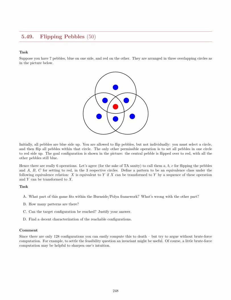
5.49. Flipping Pebbles (50)

TaskSuppose you have 7 pebbles, blue on one side, and red on the other. They are arranged in three overlapping circles asin the picture below.

Initially, all pebbles are blue side up. You are allowed to flip pebbles, but not individually: you must select a circle,and then flip all pebbles within that circle. The only other permissible operation is to set all pebbles in one circleto red side up. The goal configuration is shown in the picture: the central pebble is flipped over to red, with all theother pebbles still blue.

Hence there are really 6 operations. Let’s agree (for the sake of TA sanity) to call them a, b, c for flipping the pebblesand A, B, C for setting to red, in the 3 respective circles. Define a pattern to be an equivalence class under thefollowing equivalence relation: X is equivalent to Y if X can be transformed to Y by a sequence of these operationand Y can be transformed to X.

Task

A. What part of this game fits within the Burnside/Polya framework? What’s wrong with the other part?

B. How many patterns are there?

C. Can the target configuration be reached? Justify your answer.

D. Find a decent characterization of the reachable configurations.

CommentSince there are only 128 configurations you can easily compute this to death – but try to argue without brute-forcecomputation. For example, to settle the feasibility question an invariant might be useful. Of course, a little brute-forcecomputation may be helpful to sharpen one’s intuition.

248

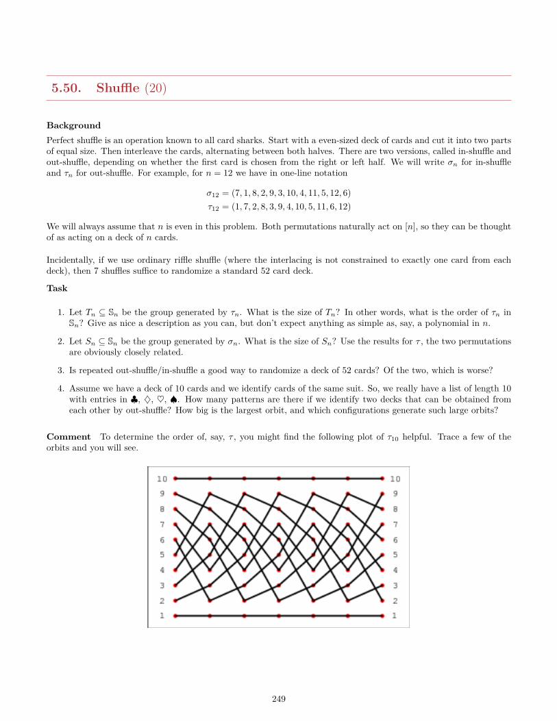
5.50. Shuffle (20)

BackgroundPerfect shuffle is an operation known to all card sharks. Start with a even-sized deck of cards and cut it into two partsof equal size. Then interleave the cards, alternating between both halves. There are two versions, called in-shuffle andout-shuffle, depending on whether the first card is chosen from the right or left half. We will write σn for in-shuffleand τn for out-shuffle. For example, for n = 12 we have in one-line notation

σ12 = (7, 1, 8, 2, 9, 3, 10, 4, 11, 5, 12, 6)τ12 = (1, 7, 2, 8, 3, 9, 4, 10, 5, 11, 6, 12)

We will always assume that n is even in this problem. Both permutations naturally act on [n], so they can be thoughtof as acting on a deck of n cards.

Incidentally, if we use ordinary riffle shuffle (where the interlacing is not constrained to exactly one card from eachdeck), then 7 shuffles suffice to randomize a standard 52 card deck.

Task

1. Let Tn ⊆ Sn be the group generated by τn. What is the size of Tn? In other words, what is the order of τn inSn? Give as nice a description as you can, but don’t expect anything as simple as, say, a polynomial in n.

2. Let Sn ⊆ Sn be the group generated by σn. What is the size of Sn? Use the results for τ , the two permutationsare obviously closely related.

3. Is repeated out-shuffle/in-shuffle a good way to randomize a deck of 52 cards? Of the two, which is worse?

4. Assume we have a deck of 10 cards and we identify cards of the same suit. So, we really have a list of length 10with entries in ♣, ♦, ♥, ♠. How many patterns are there if we identify two decks that can be obtained fromeach other by out-shuffle? How big is the largest orbit, and which configurations generate such large orbits?

Comment To determine the order of, say, τ , you might find the following plot of τ10 helpful. Trace a few of theorbits and you will see.

249

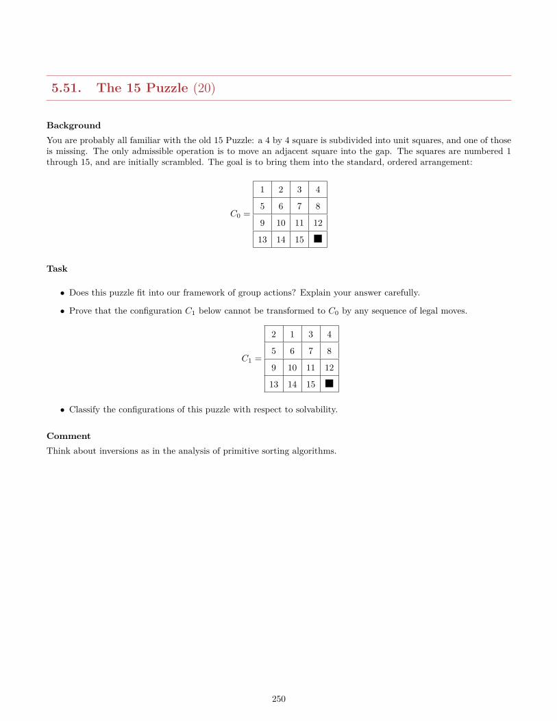
5.51. The 15 Puzzle (20)

BackgroundYou are probably all familiar with the old 15 Puzzle: a 4 by 4 square is subdivided into unit squares, and one of thoseis missing. The only admissible operation is to move an adjacent square into the gap. The squares are numbered 1through 15, and are initially scrambled. The goal is to bring them into the standard, ordered arrangement:

C0 =

1 2 3 4

5 6 7 8

9 10 11 12

13 14 15

Task

• Does this puzzle fit into our framework of group actions? Explain your answer carefully.

• Prove that the configuration C1 below cannot be transformed to C0 by any sequence of legal moves.

C1 =

2 1 3 4

5 6 7 8

9 10 11 12

13 14 15

• Classify the configurations of this puzzle with respect to solvability.

CommentThink about inversions as in the analysis of primitive sorting algorithms.

250

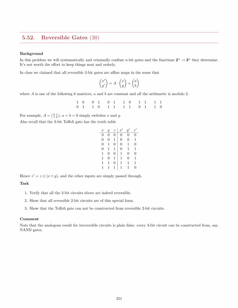
5.52. Reversible Gates (30)

BackgroundIn this problem we will systematically and criminally confuse n-bit gates and the functions 2n → 2n they determine.It’s not worth the effort to keep things neat and orderly.

In class we claimed that all reversible 2-bit gates are affine maps in the sense that(x′

y′

)= A ·

(xy

)+(ab

)where A is one of the following 6 matrices, a and b are constant and all the arithmetic is modulo 2.

1 00 1

0 11 0

0 11 1

1 01 1

1 10 1

1 11 0

For example, A = ( 0 11 0 ), a = b = 0 simply switches x and y.

Also recall that the 3-bit Toffoli gate has the truth table

x y z x′ y′ z′

0 0 0 0 0 00 0 1 0 0 10 1 0 0 1 00 1 1 0 1 11 0 0 1 0 01 0 1 1 0 11 1 0 1 1 11 1 1 1 1 0

Hence z′ = z ⊕ (x ∧ y), and the other inputs are simply passed through.

Task

1. Verify that all the 2-bit circuits above are indeed reversible.

2. Show that all reversible 2-bit circuits are of this special form.

3. Show that the Toffoli gate can not be constructed from reversible 2-bit circuits.

CommentNote that the analogous result for irreversible circuits is plain false: every 3-bit circuit can be constructed from, say,NAND gates.

251

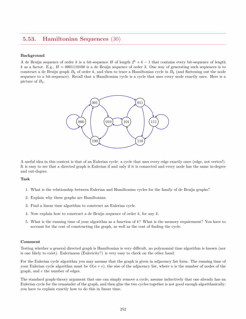
5.53. Hamiltonian Sequences (30)

BackgroundA de Bruijn sequence of order k is a bit-sequence H of length 2k + k − 1 that contains every bit-sequence of lengthk as a factor. E.g., H = 0001110100 is a de Bruijn sequence of order 3. One way of generating such sequences is toconstruct a de Bruijn graph Bk of order k, and then to trace a Hamiltonian cycle in Bk (and flattening out the nodesequence to a bit-sequence). Recall that a Hamiltonian cycle is a cycle that uses every node exactly once. Here is apicture of B3.

001 011

000 010 101 111

100 110

A useful idea in this context is that of an Eulerian cycle: a cycle that uses every edge exactly once (edge, not vertex!).It is easy to see that a directed graph is Eulerian if and only if it is connected and every node has the same in-degreeand out-degree.

Task

1. What is the relationship between Eulerian and Hamiltonian cycles for the family of de Bruijn graphs?

2. Explain why these graphs are Hamiltonian.

3. Find a linear time algorithm to construct an Eulerian cycle.

4. Now explain how to construct a de Bruijn sequence of order k, for any k.

5. What is the running time of your algorithm as a function of k? What is the memory requirement? You have toaccount for the cost of constructing the graph, as well as the cost of finding the cycle.

CommentTesting whether a general directed graph is Hamiltonian is very difficult, no polynomial time algorithm is known (noris one likely to exist). Eulerianess (Eulericity?) is very easy to check on the other hand.

For the Eulerian cycle algorithm you may assume that the graph is given in adjacency list form. The running time ofyour Eulerian cycle algorithm must be O(n+ e), the size of the adjacency list, where n is the number of nodes of thegraph, and e the number of edges.

The standard graph-theory argument that one can simply remove a cycle, assume inductively that one already has anEulerian cycle for the remainder of the graph, and then glue the two cycles together is not good enough algorithmically:you have to explain exactly how to do this in linear time.

252

5.54. Counting Boolean Circuits (25)

BackgroundGiven a circuit that computes some particular Boolean function one can easily modify input and output channels toobtain other Boolean functions. For example, we might rotate or even permute inputs and/or flip some of the bits.This leads to lots of counting problems: count Boolean functions on k inputs modulo some equivalence. Here are someexamples.

Task

A. Count the number of equivalent Boolean functions on k inputs when inputs and the output can be inverted.

B. Count the number of equivalent Boolean functions on k inputs when inputs can be arbitrarily permuted:

f(x1, x2, . . . , xk) = g(xπ(1), xπ(2), . . . , xπ(k))

where π is any permutation of [k].

C. Count the number of equivalent Boolean functions on k inputs if the inputs can be rotated. So if the rotationis by one place to the left we have

f(x1, x2, . . . , xk) = g(x2, x3, . . . , xk, x1)

D. Count the number of equivalent Boolean functions on k inputs if the inputs can be rotated and inverted.

CommentFor the last three problems don’t try to come up with simple closed-form solutions; they don’t exist. But try to writedown the answer concisely and elegantly.

253

5.55. Four Fours (50)

BackgroundThere are many problems of the type “given such-and-such arithmetic operations and numbers such-and-such, showhow to get value this-and-that”. For the most part, these puzzles are quite boring, but they provide and excellentexcuse to implement some algorithms that manipulate and evaluate arithmetic expressions.For the following problem the admissible operations are plus, minus, times, divide, exponentiate, factorials and squareroots. Admissible constants are 4, 4, 4, 4; each of the four instances of 4 must be used. The goal is to represent allpositive integers up to 100.For example, 3 = (4 + 4 + 4)/4 and 63 = (44 − 4)/4.

Task

A. How many integers can be written using only the five binary operators?

B. Add the two unary operators; how many integers can be expressed now?

C. Lastly, add the two hoaky operations .4 (put a decimal point in front of a 4) and .4 = 0.4444 . . . = 4/9. Can younow obtain all numbers up to 100?

CommentTry to find an elegant approach, avoiding unnecessarily large searches. Some people have driven the search forfour-fours expressions much further, and are allowing absurdly complicated functions in the process.

254

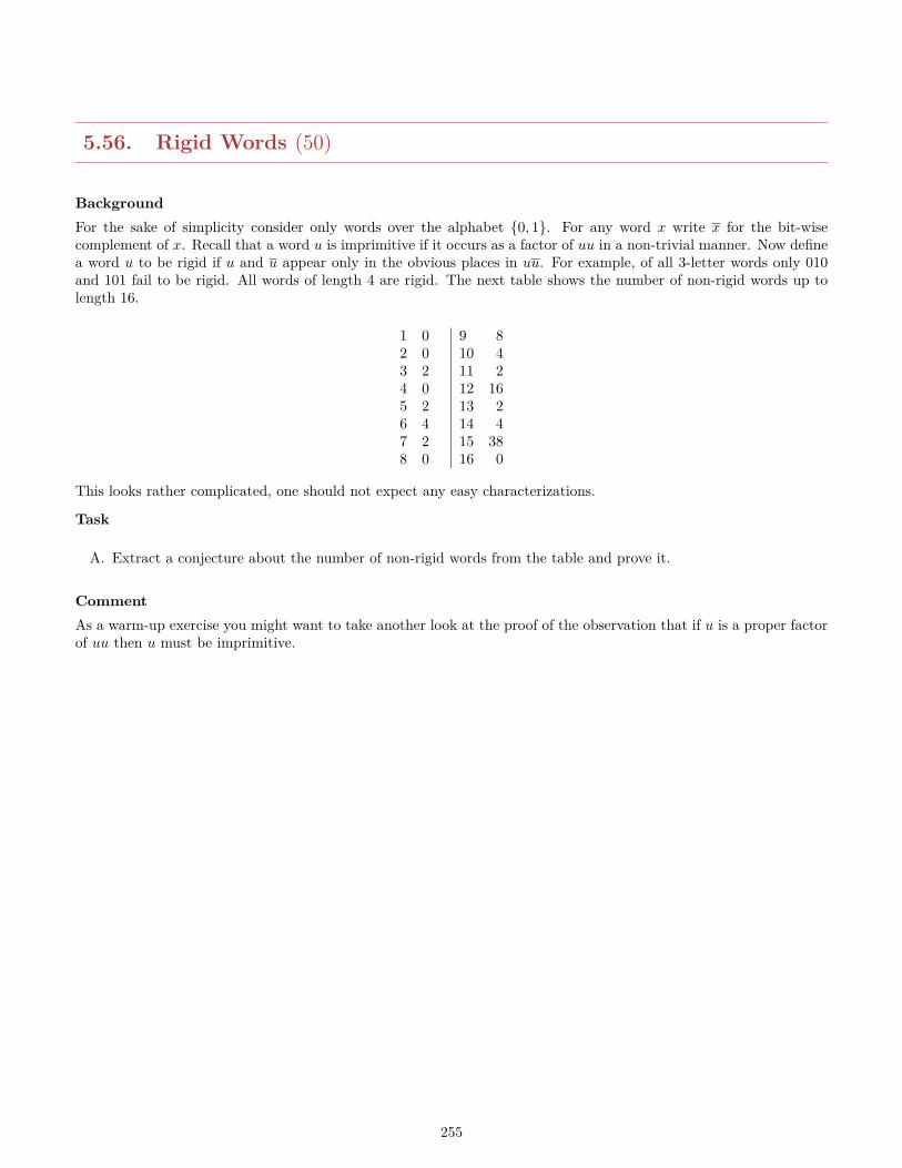
5.56. Rigid Words (50)

BackgroundFor the sake of simplicity consider only words over the alphabet 0, 1. For any word x write x for the bit-wisecomplement of x. Recall that a word u is imprimitive if it occurs as a factor of uu in a non-trivial manner. Now definea word u to be rigid if u and u appear only in the obvious places in uu. For example, of all 3-letter words only 010and 101 fail to be rigid. All words of length 4 are rigid. The next table shows the number of non-rigid words up tolength 16.

1 0 9 82 0 10 43 2 11 24 0 12 165 2 13 26 4 14 47 2 15 388 0 16 0

This looks rather complicated, one should not expect any easy characterizations.

Task

A. Extract a conjecture about the number of non-rigid words from the table and prove it.

CommentAs a warm-up exercise you might want to take another look at the proof of the observation that if u is a proper factorof uu then u must be imprimitive.

255

5.57. Keane Products (50)

BackgroundFor the sake of simplicity consider only words over the alphabet 0, 1. For any word x write x for the bit-wisecomplement of x. Define the Keane product on binary words as follows.

u× ε = ε

u× v0 = (u× v)uu× v1 = (u× v)u

For example, 001× 10 = 110001. Since Keane multiplication is associative (see part (A) below) we can form arbitraryfinite products without worrying about parentheses. How about infinite products, say

v0 × v1 × v2 × v3 × . . .

In general, one cannot make sense out of this product since the initial segments Vn = v0 × v1 . . . vn fail to converge.However, if all vi, i > 0, start with a 0 (and v0 6= ε) then Vn is a proper prefix of Vn+1 and the sequence (Vn) has anatural limit V ∈ 2ω. This construction is interesting even vi = v for all i. For example,

uω = u× 0× 0× 0 . . .(10)ω = 1× 010× 010× 010 . . .

011010011001011010010110011 . . . = 01× 01× 01× 01 . . .001001110001001110110110001 . . . = 001× 001× 001× 001 . . .

The first and last infinite word are periodic, but the second is the famous Morse-Thue word and has a rather complicatestructure (for example, it is cube-free).

Task

A. Show that multiplication is associative: u× (v × w) = (u× v)× w.

B. Determine for which multipliers vi the product word V ∈ 2ω is periodic.

CommentThe second part is hard, but the examples given above are ever so helpful. Assume V = uω where u has minimallength; compare the lengths of u and Vn.

256

5.58. Counting Cubes (50)

BackgroundWe have seen in class that the dihedral group D4 describes all rigid motions that move a square back to itself, includingreflections. This and similar dihedral groups together with the Polya machinery are very helpful to solve a variety of“two-dimensional” counting problems. There is an obvious three-dimensional analogue based on the group G of rigidmotions that moves a cube back to itself. There is a natural subgroup H that excludes reflections (so there are onlyrotations to deal with).

Task

A. Find a (small) set of generators for H. What is the size of H?

B. Find a (small) set of generators for G. What is the size of G?

C. How do the group elements act as permutations on the set of vertices of a cube?

D. Determine the cycle index polynomial of H and G.

Extra Credit: Find a minimal set of generators and describe the equations that hold between these generatorsanalogous to our description of Dn as an = 1, ab = ban−1.Extra Credit: Determine the pattern inventory for H and G. Unless you are Gauss, you probably want to usecomputer algebra to do this.

CommentIf you have perfect geometric intuition you can do this with a piece of paper and a pencil. If not, it might be a goodidea to use a physical model of a cube (like a Rubik’s cube) to make sure you get the operations right.

257

5.59. A Hamming Code (50)

BackgroundWe have seen that Hamming codes can be constructed for all arities q = pk and redundancies r (in a reasonablerange), yielding codes of minimum distance 3. The binary case is arguably the most important, but other arities arealso useful.In the following we deal with a quinary code (q = p = 5).

Task

A. Construct the check matrix of a quinary Hamming [6, 4] code.

B. Construct the corresponding generator matrix.

C. Give an example that shows that your code cannot correct 2 errors.

CommentTo avoid chaos, let’s adopt the convention that the first non-zero entry in each column of the check matrix is 1.

258

5.60. Tournaments (50)

BackgroundConsider a round-robin tournament with n players (all participants play against each other in all possible pairings).We can model a tournament nicely by imposing an arbitrary orientation on a complete graph Kn on n points: adirected edge x→ y means that x beats y. Let us say that x dominates y if there is a path from x to y in this graph.Note that our graphs are unlabeled, we ignore the names of the players.It is difficult to compare the relative strength of players; for example, it may well happen that two players dominateeach other. Define a comparison “weaker than” on T by setting x ≺ y if y beats x but x does not dominate y. Atournament is orderly if no two players dominate each other. By contrast, a tournament is chaotic if any two playersdominate each other. A leader in a tournament is a player that dominates all other players. A strong leader is a leaderwhere all the corresponding paths have length at most 2.Suppose we have an ordering π : v1, v2, . . . , vn of the vertices. Call a pair (i, j) where i < j and vj beats vi a defect ofcost j − i and let D(π) be the sum of all these costs.

Task

A. Show that ≺ is a strict partial order.

B. Find all tournaments with four players, up to isomorphism.

C. Show that for every n there is only one orderly tournament, up to isomorphism.

D. Show that an arbitrary tournament has a leader.

E. Show that an arbitrary tournament has a strong leader.

F. Prove or disprove: In an arbitrary tournament, every node of maximal out-degree is a leader.

G. Show that every tournament has a Hamiltonian path.

H. Show that a tournament is chaotic iff it has a Hamiltonian cycle.

I. Show that, for any ordering π that minimizes D(π), player vi has at least as many wins as player vi+1, for alli < n.

Comment

259

5.61. Sinkerator (50)

BackgroundSuppose G is a loop-free directed graph on n nodes, represented an adjacency matrix. A deep-sink in G is a vertex ofin-degree n− 1 and out-degree 0. Note that a deep-sink is unique, if it exists at all.

Task

A. Find an algorithm to determine the existence of a deep-sink that is better than Ω(n2).

B. Prove correctness of your algorithm and determine its running time.

Comment

260

5.62. Degrees (50)

BackgroundEvery undirected graph G on n points is associated with its degree sequence ∆(G), the list d1, d2, . . . , dn of thedegrees of all the vertices in G, sorted in non-increasing order. An arbitrary sequence of natural numbers is graphicalor realizable if there is a graph G such that ∆(G) is the given sequence. For example, 3, 2, 2, 1 and 2, 2, 2, 2 arerealizable, but 3, 3, 3, 1 is not (which means, by the way, that in any graph realizing the first sequence, the two degree2 vertices must be adjacent).Here is a well-known result by Havel and Hakimi: let d = d1, d2, . . . , dn be a non-increasing list of natural numberswhere n ≥ 2. Abbreviate k = d1 and define d′ = d2 − 1, . . . , dk+1 − 1, dk+2 . . . , dn (reorder if necessary). Then d isgraphical iff d′ is graphical.Suppose xy and zw are edges in a graph G, but xw and zy are not. A 2-switch is an operation that removes xy andzw, and adds xw and zy. Note that a 2-switch does not change the degree sequence of G.One might wonder how many entries in a realizable sequence can be distinct. Call a realizable degree sequenceheterogeneous if it has as many different entries as possible. Likewise, a graph is heterogeneous if its degree sequenceis.

Task

A. Show that for any graph of size n ≥ 2 there must be two vertices with the same degree.

B. Find a family of heterogeneous graphs for all sizes n.

C. Characterize all heterogeneous graphs.

D. Prove the Havel-Hakimi theorem.

E. Show that graphs with the same degree sequence can be transformed into one another by a series of 2-switches.

Comment For part (B) it is a good idea to enumerate a few small examples. Then ponder deeply and do not forgetto show that your answer captures all the proper graphs.

261

5.63. Forests in a Tree (50)

BackgroundIn the following let T be a finite tree. We will consider families (Ti)i≤n of non-empty subtrees of T . Let’s call such afamily pairwise overlapping if i < j implies that Ti ∩ Tj 6= ∅. The whole family is overlapping if

⋂Ti 6= ∅.

Task

A. Show that T1 ∪ T2 is a tree iff T1 ∩ T2 6= ∅.

B. Show that any pairwise overlapping family is already overlapping.

Comment

262

5.64. Graph Partitions (50)

BackgroundA ugraph G is bipartite if there is a partition V = X ∪ Y of the vertex set such that all edges in G connect X and Y .In general, we write G[X,Y ] for the subgraph of G whose edges connect X and Y . Note that this graph is spanning.By a decomposition of G we mean a family F1, . . . , Fk of edge-disjoint subgraphs of G such that

⋃E(Fi) = E(G). We

are here only interested in decompositions of Kn by complete bipartite graphs Kk,`.A graph is even if all its vertices have even degree.

Task

A. Show that a graph is bipartite iff it has no odd-length cycle.

B. Clearly G[X,Y ] = G[Y,X]. Other than this obvious symmetry, is the partition of a bipartite graph unique?

C. Show that every ugraph G such that∑(

d(v)2)>(n2)

has a 4-cycle.

D. Show that every ugraph G admits a spanning bipartite subgraph H = G[X,Y ] such that dH(v) ≥ dG(v)/2 forall v.

E. Find a small decomposition of Kn into stars Kk,1.

F. Show every decomposition of Kn has at least n− 1 elements.

G. A graph is even iff it admits a cycle decomposition.

Comment

263

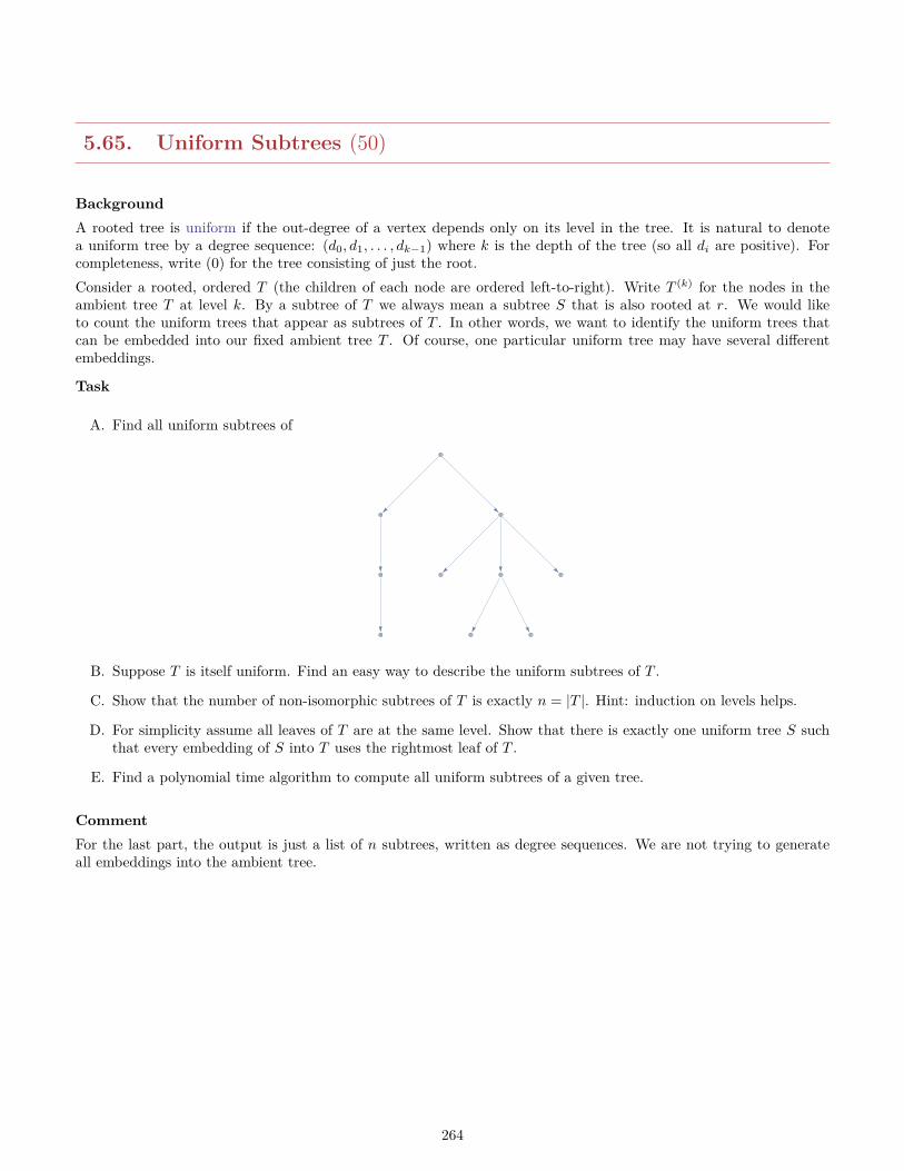
5.65. Uniform Subtrees (50)

BackgroundA rooted tree is uniform if the out-degree of a vertex depends only on its level in the tree. It is natural to denotea uniform tree by a degree sequence: (d0, d1, . . . , dk−1) where k is the depth of the tree (so all di are positive). Forcompleteness, write (0) for the tree consisting of just the root.Consider a rooted, ordered T (the children of each node are ordered left-to-right). Write T (k) for the nodes in theambient tree T at level k. By a subtree of T we always mean a subtree S that is also rooted at r. We would liketo count the uniform trees that appear as subtrees of T . In other words, we want to identify the uniform trees thatcan be embedded into our fixed ambient tree T . Of course, one particular uniform tree may have several differentembeddings.

Task

A. Find all uniform subtrees of

B. Suppose T is itself uniform. Find an easy way to describe the uniform subtrees of T .

C. Show that the number of non-isomorphic subtrees of T is exactly n = |T |. Hint: induction on levels helps.

D. For simplicity assume all leaves of T are at the same level. Show that there is exactly one uniform tree S suchthat every embedding of S into T uses the rightmost leaf of T .

E. Find a polynomial time algorithm to compute all uniform subtrees of a given tree.

CommentFor the last part, the output is just a list of n subtrees, written as degree sequences. We are not trying to generateall embeddings into the ambient tree.

264

5.66. Eccentricity (50)

BackgroundLet G be a ugraph. For any vertex u, its eccentricity is defined to be e(u) = max

(dist(u, x) | x ∈ V

). The eccentricity

of G is e(G) = min(e(x) | x ∈ V

). A central vertex of G is a vertex u such that e(u) = e(G); Z(G) is the collection

of all central vertices.To avoid tedious special cases assume below that T is a tree on at least 3 points. Write T ′ for the tree obtained fromT by removing all leaves.

Task

A. Let e(u) = dist(u, v). Then v is a leaf.

B. Show that eT (u) = eT ′(u) + 1.

C. Show that Z(T ) = Z(T ′).

D. Show that a tree has either one or two central vertices; in the second case they are adjacent.

E. Show that every automorphism of a tree fixes a vertex or an edge.

F. Find a fast algorithm to compute the eccentricity and the central vertices of a tree. Analyze the running timeof your method.

Comment

265

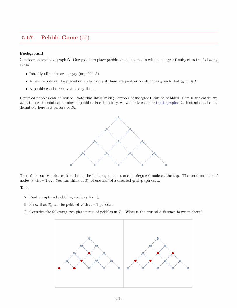
5.67. Pebble Game (50)

BackgroundConsider an acyclic digraph G. Our goal is to place pebbles on all the nodes with out-degree 0 subject to the followingrules:

• Initially all nodes are empty (unpebbled).

• A new pebble can be placed on node x only if there are pebbles on all nodes y such that (y, x) ∈ E.

• A pebble can be removed at any time.

Removed pebbles can be reused. Note that initially only vertices of indegree 0 can be pebbled. Here is the catch: wewant to use the minimal number of pebbles. For simplicity, we will only consider trellis graphs Tn. Instead of a formaldefinition, here is a picture of T5:

Thus there are n indegree 0 nodes at the bottom, and just one outdegree 0 node at the top. The total number ofnodes is n(n+ 1)/2. You can think of Tn of one half of a directed grid graph Gn,n.

Task

A. Find an optimal pebbling strategy for T4.

B. Show that Tn can be pebbled with n+ 1 pebbles.

C. Consider the following two placements of pebbles in T5. What is the critical difference between them?

266

D. Show that the optimal pebbling strategy for Tn requires n+ 1 pebbles.

Comment

267

5.68. Flipping Pebbles (50)

BackgroundAn interesting class of problems deals with the question whether a certain system can ever reach a particular state,given a collection of possible transitions the system can make.As an example, consider a collection of tokens, blue on one side, and red on the other. We have 2n tokens aligned ona 2× n grid, initially all tokens are blue side up. The admissible transitions are described as follows:

Pick an arbitrary token, and flip it over; also, flip over its two neighbors.

Can the system reach the all-red state?

Task

A. Show that order of the flip operations does not matter.

B. Show that flipping the same token twice undoes the first flip, and so two flips have no effect.

C. Show that all 2×n grids of tokens can reach the the all-red state by flipping tokens and their neighbors, startingfrom all-blue.

D. (Extra Credit) Repeat for 3× n grids.

Comment This actually works for arbitrary m× n grids, but the proof is much harder.

268

Chapter 6

Finite State Machines

269

6.1. Longest Common Prefix (50)

BackgroundLet W be a string of length n and assume we already have the suffix array SA and the longest common prefixarray LCP. For i < j, define lcp(i, j) to be the length of the longest common prefix of suffixes SA(i) and SA(j), soLCP(i) = lcp(i, i+ 1).We will show how to use preprocessing to answer LCP queries in constant time. To this end we will use range minima:we want to quickly compute rlcp(i, j) = min(LCP(`) | i ≤ ` ≤ j), 1 ≤ i ≤ j ≤ n. For simplicity, assume LCP(i) = ∞for i > n.Define R(k, i) = min(LCP(`) | i ≤ ` < i+ 2k) where k ≤ logn.

Task

A. Suppose i < j. Show that lcp(i, j) = min(LCP(`) | ` = i, . . . , j − 1).

B. Explain how to compute all the R(k, i) efficiently. What is the time complexity or your method?

C. Given R, show how to answer LCP queries in constant time.

D. What does this have to do with the lowest common ancestor problem in the corresponding suffix tree?

Comment

270

6.2. Occurrence Counting with Suffix Arrays (50)

BackgroundLet W be a word of length n, and u a factor of W of length m. We want to tackle the problem of reporting alloccurrences of u in W , assuming we already have the suffix array SA of W and the LCP array. The obvious binarysearch approach takes time O(m logn), but is often faster (fewer than m letter-to-letter comparisons are needed).

To get a guaranteed speedup one has to cut down on the number of letter-to-letter comparisons made during thebinary search. Ideally, we would like to examine every position in u at most once. To this end, temporarily assumewe have access to a general lcp function such that lcp(i, j) is the length of the longest common prefix of suffixes SA(i)and SA(j).

Task

A. Explain how to determine all occurrences of u in time O(m logn).

B. Assuming lcp is available at constant cost, show how to modify binary search on SA to find all occurrences of uin time O(m+ logn).

C. Show how to precompute the needed lcp values in time linear in n. For simplicity, assume that n is a power of 2.

Comment

271

6.3. Maximal Palindromes (50)

Background Let W be a (long) string. A palindrome in W is a factor u of W that is a palindrome. The palindromeis maximal if it cannot be extended any further. One can find all the maximal palindromes in linear time using suffixtrees. It will be helpful to take a look at the longest common factor construction discussed in class. Also, you mayuse the fact that, after linear time preprocessing, one can answer lowest common ancestor queries in constant time.

Task

A. Explain what suffix tree one should build to tackle the maximal palindrome problem.

B. Analyze the running time of your algorithm, including all the preprocessing and the actual search for the maximalpalindromes.

Comment

272

6.4. Palindromes (50)

BackgroundA palindrome is a word that reads the same left-to-right and right-to-left. Thus abba is a palindrome, but abab is not.Suppose we have a word w over some alphabet Σ. Since single letters are palindromes, we can always find a decom-position

w = u1u2 . . . uk

where all the ui are palindromes. However, it’s not so clear how one can minimize the number k of palindromes. Thisis the palindrome decomposition problem.Slightly more challenging is the following type of decomposition based on erasing palindromes. Suppose w = xuywhere u is a palindrome. Then in one step we can rewrite w to xy. Clearly, after at most |w| steps, we can rewritew to ε, the empty word. Again, the challenge is to minimize the number of steps. This is the palindrome erasureproblem.

Task

A. Find a cubic time algorithm to solve the palindrome decomposition problem. Your algorithm should return alist of the corresponding palindromes.

B. Find a cubic time algorithm to solve the palindrome erasure problem. Your algorithm should return a list of thecorresponding erasures.

Comment You might find dynamic programming helpful.For part (B), return a list of pairs (i, j) where 1 ≤ i ≤ j ≤ |w| that indicate that one is supposed to remove thepalindrome from wi to wj . Note that there may be gaps from previous erasures, but keep the original indexing.

273

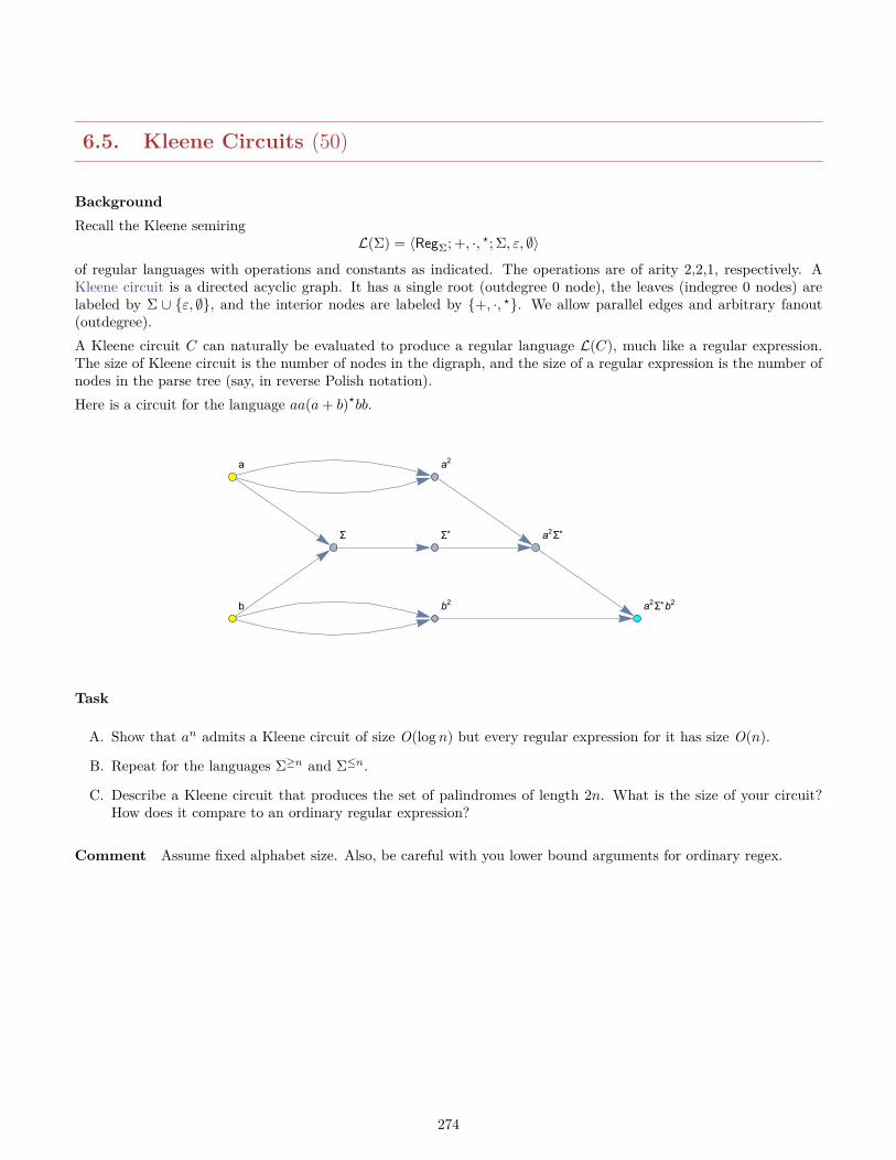
6.5. Kleene Circuits (50)

BackgroundRecall the Kleene semiring

L(Σ) = 〈RegΣ; +, ·, ?; Σ, ε, ∅〉

of regular languages with operations and constants as indicated. The operations are of arity 2,2,1, respectively. AKleene circuit is a directed acyclic graph. It has a single root (outdegree 0 node), the leaves (indegree 0 nodes) arelabeled by Σ ∪ ε, ∅, and the interior nodes are labeled by +, ·, ?. We allow parallel edges and arbitrary fanout(outdegree).A Kleene circuit C can naturally be evaluated to produce a regular language L(C), much like a regular expression.The size of Kleene circuit is the number of nodes in the digraph, and the size of a regular expression is the number ofnodes in the parse tree (say, in reverse Polish notation).Here is a circuit for the language aa(a+ b)?bb.

a

Σ

b

a2

b2

Σ*

a2Σ*

a2Σ*b2

Task

A. Show that an admits a Kleene circuit of size O(logn) but every regular expression for it has size O(n).

B. Repeat for the languages Σ≥n and Σ≤n.

C. Describe a Kleene circuit that produces the set of palindromes of length 2n. What is the size of your circuit?How does it compare to an ordinary regular expression?

Comment Assume fixed alphabet size. Also, be careful with you lower bound arguments for ordinary regex.

274

6.6. Quasiperiodic Words (50)

BackgroundA word w is a quasiperiod of a non-empty word v if v = ww . . .w where denotes fusion. More precisely, xy = zif there are words x′, y′ and u such that x = x′u, y = uy′ and z = x′y′. Thus x and y overlap in u and instead ofplain concatenation we superimpose these two occurrences of u. Note that concatenation is the special case where uis empty. Strictly speaking, x y is multi-valued rather than a function, but we won’t quibble. In this problem we willtake a few first steps towards discussing the language Qw of words have w as a quasiperiod. A language L is monoidalif L = L? (equivalently, ε ∈ L and LL ⊆ L). Given a monoidal language L, its star root, in symbols ∗

√L, is the least

language K such that K? = L.Let

Pw = x | x 6= ε, x v w < xw .

For example, for w = aabaa we have Pw = ∗√Pw

? = aab, aaba, aabaa and the first few words in Qw are

aabaa, aabaabaa, aabaaabaa, aabaabaabaa, aabaaabaabaa, aabaabaaabaa, aabaaabaaabaa, aabaabaabaabaa

Task

A. Show that Pw = x | |x| ≤ |w|, w < xω .

B. Show that Qw = Pw?w = Pw

? ∩ wΣ?.

C. Show that ∗√L = L0 − L2

0 where L0 = L− ε.

D. Show that all words in ∗√Pw

? are primitive.

Comment

275

6.7. Sparse Languages (50)

BackgroundA language L ⊆ Σ? is sparse if there is some polynomial p such that |L∩Σn| ≤ p(n). All tally languages L ⊆ a? aresparse. Now suppose we have a partial oder ≤ on Σ. Call a word w ∈ Σ? orderly if w = xaybz, a, b ∈ Σ, x, y, z ∈ Σ?implies a ≤ b. A language is orderly if all its words are.

Task

A. Show that a regular language is sparse if, and only if, is a finite union of languages of the form u0v1?u1v2

?u2 . . . uk−1vk?uk,

ui, vi ∈ Σ?.

B. Describe an algorithm to test whether a regular language is sparse. You may assume you have a DFA acceptingthe language.

C. What is the time and space complexity of your algorithm?

D. Show that the language of all orderly words in sparse.

276

6.8. MSO Descriptions (50)

BackgroundWe have seen in class that the regular languages are precisely the ones that can be described by a MSO[<] formula ϕ:

Lϕ = W ∈ Σ? |W |= ϕ .

To characterize languages, one uses structures consisting of a single word W ∈ Σn with positions ranging over [n]. Itis straightforward to work with several words W,U, V ∈ Σn of the same length. Let us write Qa,W (x) to mean that“word W has a letter a in position x,” and likewise for U and V .Write bin(U) for the numerical value of a word U ∈ 2? written in reverse binary. E.g., bin(01101) = 22.

Task

A. Construct a formula ϕ for the language (aa, b)?a.

B. Construct a formula ψ such that (U, V,W ) |= ψ if, and only if, bin(U) + bin(V ) = bin(W ). Recall that the wordsall have the same length, there is no overflow.

277

6.9. Star-Free Languages (50)

BackgroundRecall that a language is star-free if it can be generated from ∅, singletons a and the operations union, concatenationand complement.For example, a?b?a? and (ab)? are star-free, but (a, ba, b)? is not.

Task

A. Show that a?b?a? and (ab)? are star-free.

B. Show that every star-free language is first-order definable.

CommentThe opposite direction is also true, but much harder to prove.

278

6.10. NFA Universality (30)

BackgroundFor a DFA, the Universality Problem L(M) = Σ? can be solved by graph exploration in linear time. But for nonde-terministic machines things become much more complicated. The obvious approach is to determinize the machine;alas, that can cause exponential blowup.

Task

A. Show that NFA Universality is in PSPACE.

B. Show that NFA Universality is PSPACE-complete.

CommentFor hardness, construct a reduction from Pointed Rectangular Tiling.

279

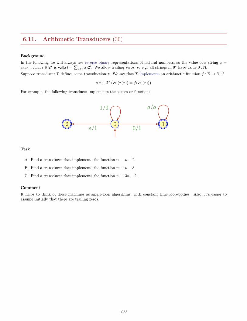
6.11. Arithmetic Transducers (30)

BackgroundIn the following we will always use reverse binary representations of natural numbers, so the value of a string x =x0x1 . . . xn−1 ∈ 2? is val(x) =

∑i<n xi2i. We allow trailing zeros, so e.g. all strings in 0? have value 0 : N.

Suppose transducer T defines some transduction τ . We say that T implements an arithmetic function f : N→ N if

∀x ∈ 2?(val(τ(x)) = f(val(x))

)For example, the following transducer implements the successor function:

2 0 1ε/1 0/1

1/0 a/a

Task

A. Find a transducer that implements the function n 7→ n+ 2.

B. Find a transducer that implements the function n 7→ n+ 3.

C. Find a transducer that implements the function n 7→ 3n+ 2.

CommentIt helps to think of these machines as single-loop algorithms, with constant time loop-bodies. Also, it’s easier toassume initially that there are trailing zeros.

280

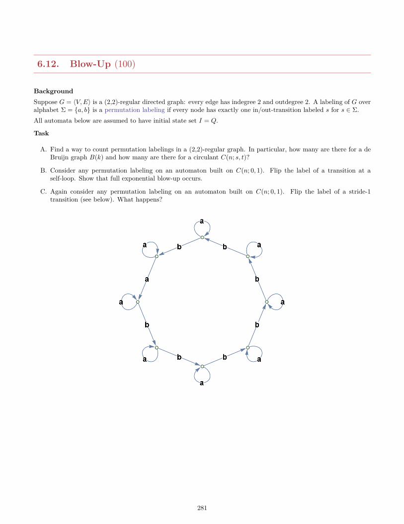
6.12. Blow-Up (100)

BackgroundSuppose G = 〈V,E〉 is a (2,2)-regular directed graph: every edge has indegree 2 and outdegree 2. A labeling of G overalphabet Σ = a, b is a permutation labeling if every node has exactly one in/out-transition labeled s for s ∈ Σ.All automata below are assumed to have initial state set I = Q.

Task

A. Find a way to count permutation labelings in a (2,2)-regular graph. In particular, how many are there for a deBruijn graph B(k) and how many are there for a circulant C(n; s, t)?

B. Consider any permutation labeling on an automaton built on C(n; 0, 1). Flip the label of a transition at aself-loop. Show that full exponential blow-up occurs.

C. Again consider any permutation labeling on an automaton built on C(n; 0, 1). Flip the label of a stride-1transition (see below). What happens?

281

6.13. Reversibility of ECA (30)

BackgroundSuppose ρ : 23 → 2 is the local map of an elementary cellular automaton. We have seen how to construct fromρ a synchronous transducer A_,x,y that checks whether a finite bit sequence x evolves to y in one step under fixedboundary conditions. Naturally, there is a similar machine for cyclic boundary conditions.Reversibility of a cellular automaton is expressed by the FO formula

ϕ′ ≡ ∀x, y, z (x_ z ∧ y _ z ⇒ x = y)

It is sligthly easier to work with irreversibility, expressed by the negation ϕ = ¬ϕ′. The finite case here is muchmessier than the biinfinite case, so let’s work with configurations Z→ 2.

Task

A. Construct a synchronous 2-track transducer B_ that checks whether a finite bit sequence x evolves to y in onestep under cyclic boundary conditions.

B. Then build a synchronous 3-track transducer A that accepts the language defined by the matrix of ϕ. Whatdoes A have to do with injectivity of the global map on 2n?

C. Explain how one can directly construct a 2-track transducer A′ that still can be used to check ϕ. This machineshould be of the form A′ = A0 × U where U is the un-equal transducer on 2 tracks.

CommentFor part (A), nondeterminism is critical (see the construction for the fixed boundary condition case). You can thinkof the step from A to A′ as eliminating the z-track.

282

6.14. Odd Parts (50)

BackgroundDefine the “odd part” operation odd : Σ+ → Σ+ by

odd(x1x2 . . . xn) = x1x3 . . . x2dn/2e−1

odd naturally extends to languages.For any modulus m ≥ 2 and remainder 0 ≤ r < m, let

Lr,m = x ∈ a, b? | #ax = r (mod m)

and set Kr,m = odd(Lr,m).

Task

A. Show that odd(L) is regular whenever L is regular.

B. Show that Kr,m is cofinite.

C. Determine the length κr,m of a longest word in the complement of Kr,m.

D. Directly construct a DFA for Kr,m (building an NFA first might help).

CommentIt seems difficult to determine the cardinality of the complement of Kr,m. Extra credit.

283

6.15. Window Languages (40)

BackgroundIn this problem we only consider languages in Σ+, so the empty word causes no technical problems. A language L isa window language if membership in L can be tested by sliding a window of size 2 across the word and observing the2-factors of the word.Here is a formalization of this idea. Define fact2(x) = ab ∈ Σ2 | x = uabv, u, v ∈ Σ? to be the set of all 2-factors ofx. Define an equivalence relation ≈ on Σ+ as follows:

x ≈ y ⇐⇒ x1 = y1 ∧ fact2(x) = fact2(y) ∧ x−1 = y−1

Then L is a window language if it saturates ≈: L =⋃x∈L[x]. Write Σ++ for all words of length at least 2. Given

F ⊆ Σ2 let LF = x ∈ Σ++ | fact2(x) ⊆ F .

Task

A. Find a fast algorithm to check whether LF is finite. What is the running time of your algorithm?

B. Find a simple, infinite language L ⊆ Σ++ that is not of the form LF .

C. Show that ≈ is a congruence: an equivalence relation such that x ≈ y implies uxv ≈ uyv for all u, v ∈ Σ?.

D. Show that every window language is regular.

E. Show that every regular language is a homomorphic image of a window language.

CommentFor the last part you need to produce a regular languageR ⊆ Γ? for some alphabet Γ and a homomorphism Φ : Γ? → Σ?such that Φ(R) = L. Γ will depend strongly on a DFA for the given regular language.This is perhaps a little counterintuitive: the window seems to be too narrow for arbitrary regular languages withlong-distance constraints (say, every a is followed by a b after at most 123 letters).

284

6.16. Primitive Words (50)

BackgroundLet w be a non-empty word. A word z is the root of w if w ∈ z? but there is no shorter word with this property. Aword is primitive if it is its own root.For example, ab is the root of abababab. The primitive words of length 3 over a, b are aab, aba, abb, baa, bab, bba.

Task

A. Show that any two non-empty words u, v that commute, uv = vu, have the same root.

B. Show that any two non-empty words u and v commute iff they have equal powers: uk = v` for positive k and l.

C. Show that a non-empty word w is primitive if, and only if, w2 = xwy implies that x = ε or y = ε.

D. Count the number of primitive words of length n over a k letter alphabet.

E. As part of some algorithm it is necessary to store a few thousand binary words of length 20. Prof. Dr.Wurzelbrunft suggests to speed things up by storing the roots of words, rather than the words directly. Whatprofessional advice can you give Wurzelbrunft?

Comment

285

6.17. Dense Languages (50)

BackgroundWrite x < y for x is lexicographically less than y where x, y ∈ Σ?. A language L ⊆ Σ? is dense if

∀x, y ∈ L (x < y ⇒ ∃ z ∈ L (x < z < y))

For example, the language L = (a+ c)?b is dense. For words in L up to length 5, lexicographic order looks like so:

aaaab, aaab, aaacb, aab, aacab, aacb, aaccb, ab, acaab, acab, acacb, acb, accab, accb, acccb, b,

caaab, caab, caacb, cab, cacab, cacb, caccb, cb, ccaab, ccab, ccacb, ccb, cccab, cccb, ccccb (6.1)

Task

A. Show that the binary language L = (a+ c)?b is dense. In fact, L is order-isomorphic to the rationals.

B. Show that for all words u < v < w the language Lu,v,w = (u+ w)?v is dense.

C. Find a way to test whether the language of a given DFA is dense.

D. What is the complexity of your decision algorithm? Assume the alphabet is fixed.

Comment

286

6.18. Word Periods (50)

BackgroundA positive integer p is a period of a non-empty word word w = w1w2 . . . wn if for all i ≤ n − p we have wp+i = wi.The least such p is referred to as the period of w.Let u be primitive and w arbitrary. The u-stable normal form of w is a decomposition of w defined as follows. If u2

is not a factor, the decomposition is just w. Otherwise we write

w = v0uα1v1u

α2 . . . uαkvk

where k ≥ 1 is minimal subject to the following constraints: the vi must not contain a factor u2 and v0 ∈ Σ?u,vi ∈ (Σ?u ∩ uΣ?) for 1 ≤ i < k and vk ∈ uΣ?.For example, for u = aba and w = ab(aba)5ba(aba)4ba we have w = ababa (aba)3 ababa(aba)3ababa.

Task

A. Let p be the period of w and u the prefix of w of length p. Show that w = uku− for some k ≥ 1 and u− a properprefix of u.

B. Again let p be the period of w and u the prefix of w of length p. Show that w is primitive if, and only if,w /∈ uuu?.

C. Show that the u-stable normal form exists and is unique.

CommentThe u-stable normal form may seem a bit strange; it turns out to be very useful in the discussion of word equations.

287

6.19. Regex Converter (40)

BackgroundPerhaps the most important application of finite state machines is pattern matching in strings: given a regularexpression α one constructs a finite state machine Mα that accepts the language described by α. One can then runMα on some input string to check whether it conforms to the pattern. There are many ways to organize the translationfrom regular expression to machine; here is one that is easy to explain and implement, and that produces reasonablygood results.A NFAE is a begin-exit automaton (BEFA) if it has precisely one initial state b, one final state e and there are notransitions starting at e and no transitions ending at b.

Task

A. Show how to construct a BEFA Mα for every regular expression α (use induction on α).

B. Show that your construction from part (A) is correct: explain exactly where your construction uses the restric-tions on transitions in a BEFA.

C. What is the size of your Mα in terms of the size of α?

D. Can you think of ways to streamline the construction of Mα a bit? Of course, if your construction in part (A)is already perfect this part is superfluous.

Comment There are other constructions that avoid ε-moves, but they are more complicated.

288

6.20. Converting Regular Expressions (50)

BackgroundWe have seen two methods for converting regular expressions to finite state machines, one due to Thompson and theother to McNaughton and Yamada.

Task

A. Convert the following rational expressions to NFAs, using both the Thompson and the McNaughton-Yamadaapproach for each expression. You might wish to recycle some of the component machines. Which method yieldsbetter results?

• aaaab∗,• (a+ b)3,• (aa+ bb+ (ab+ ba)(aa+ bb)∗(ab+ ba))∗.

B. Convert the NFAs to DFAs. Which machines are smaller?

Comment

289

6.21. Regularity and Language Operations (50)

BackgroundWe have seen that regular languages are closed under the operations of union, concatenation and Kleene star. Goingin the opposite direction is a bit more complicated.

TaskDetermine whether the following propositions are true or false. Provide a clear proof for your claim in each case.

A. L1 ∪ L2 regular and |L1| = 1 implies L2 regular.

B. L1 ∪ L2 regular and L1 finite implies L2 regular.

C. L1 ∪ L2 regular and L1 regular implies L2 regular.

D. L1 · L2 regular and |L1| = 1 implies L2 regular.

E. L1 · L2 regular and L1 finite implies L2 regular.

F. L1 · L2 regular and L1 regular implies L2 regular.

G. L∗ regular implies L regular.

CommentIf you construct a counterexample, make it small.

290

6.22. Regularity and Palindromes (50)

Background

TaskWhich of the following languages is regular over the alphabet a, b? Justify your answer.

A. L1 = x ∈ a, b∗ | x = xr

B. L2 = xwxr | x,w ∈ a, b+

C. L3 = xxrw | x,w ∈ a, b+

Comment

291

6.23. Poly-Palindromes (50)

BackgroundA word x is a poly-palindrome if it is of the form

x = w1w2 . . . wn

where all the wi are even-length palindromes (obviously this is of no interest for arbitrary palindromes). In otherwords, a poly-palindrome can be decomposed into a sequence of even-length palindromes. Note that the decompositionis not unique in general (e.g. 001100).

Task

A. Let u v = vopu where both u and v are even-length. Then v is a poly-palindrome.

B. Let x = uy be a poly-palindrome and u 6= ε be the shortest even-length palindromic prefix of x. Then y is alsoa poly-palindrome.

C. Let x = uy be a poly-palindrome and u any even-length palindromic prefix of x. Then y is also a poly-palindrome.

CommentCompare part (A) to the classical result that commuting words u v = v u must have the same root (i.e., there is somew such that u = wk and v = wl).

292

6.24. Word Binomials (50)

BackgroundBy a subsequence of a word v = v1v2 . . . vm we mean any word u = vi1vi2 . . . vir where 1 ≤ i1 < i2 < . . . ir ≤ m is astrictly increasing sequence of indices. Thus bbc and cab are subsequences of ababacaba but cbb is not.Note that a specific word can occur multiple times as a subsequence of another. For example, aab appears 7 times inababacaba. We write (

v

u

)= C(v, u) = number of occurrences of u as a subsequence of v.

The notation is justified since “word binomials” generalize ordinary binomial coefficients:(nk

)=(an

ak

). Note that

instances of u as a subsequence of v in general overlap, e.g., C(a3, a2) = 3.

TaskLet δa,b = 1 iff a = b, 0 otherwise, and a, b ∈ Σ and u, v, ui, vi ∈ Σ?.

A. Show that (va

ub

)=(v

ub

)+ δa,b

(v

u

)B. Show that (

v1v2

u

)=

∑u=u1u2

(v1

u1

)(v2

u2

)C. Give an efficient algorithm to compute word binomials.

D. Give a simple description (in terms of union, concatenation and Kleene star) of the language

L = v ∈ a, b? |(v

ab

)= 3

E. Construct the minimal DFA for L.

F. Generalize: given a word u and an integer r construct a DFA that accepts

L(u, r) = v ∈ Σ? |(v

u

)= r

Is your machine always minimal?

293

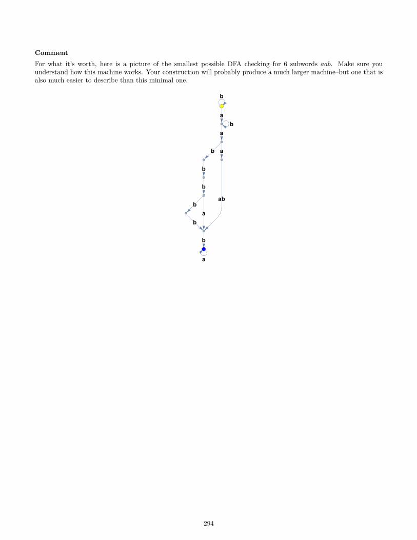
CommentFor what it’s worth, here is a picture of the smallest possible DFA checking for 6 subwords aab. Make sure youunderstand how this machine works. Your construction will probably produce a much larger machine–but one that isalso much easier to describe than this minimal one.

a

b

a

b

ab

ab

b

b

b

a

a

b

b

294

6.25. Constrained Quotients (50)

BackgroundRecall the left quotient of a language L by a word x, an inverse operation to concatenation:

x−1L = y | xy ∈ L

Suppose that L is regular. As we have seen, x−1L is also regular in this case. It is easy to see that

P (L) = x | x−1L 6= ∅

is also regular. In fact, one can constrain the length of a witness y ∈ x−1L in many ways and still obtain regularlanguages. So suppose we have a function f : N→ N and define

P (L, f) = x | x−1L ∩ Σf(|x|) 6= ∅

Let t(n) = 2n and e(n) = 2n.

Task

A. Show that P (L) is regular.

B. Show that P (L, t) is regular.

C. Show that P (L, e) is regular.

D. Give a bound on the state complexity of P (L, t) and P (L, e).

Comment

295

6.26. Word Shuffle (50)

BackgroundThe shuffle operation, in symbols ‖, is a map from Σ? × Σ? to P(Σ?) and is defined by

ε ‖ y = y ‖ ε = yxa ‖ yb = (x ‖ yb) a ∪ (xa ‖ y), b.

As usual, we extend to languages byK ‖L =

⋃x ‖ y | x ∈ K, y ∈ L

For example,aab ‖ bab = aababb, aabbab, abaabb, ababab, baaabb, baabab, babaab

and aa, bb ‖Σ? is the set of all words containing at least two a’s or b’s.Shuffle is an important idea in the study of concurrency. If we think of letters as atomic actions then the shuffle oftwo words describes all possible interleavings of two action sequences. Note that the size of the shuffle product of twowords behaves quite erratically. For example, for x = aabb and y ∈ a, b4 we get the following cardinalities:

aaaa 15 baaa 30aaab 10 baab 18aaba 12 baba 23aabb 6 babb 12abaa 19 bbaa 36abab 11 bbab 19abba 18 bbba 30abbb 10 bbbb 15

Task

A. Given two words x and y over disjoint alphabets, construct a DFA that recognizes x ‖ y. Make sure to give anice geometric description of your machine.

B. What is the connection between your DFA and binomial coefficients?

C. Given two finite state machines M1 and M2 over the same alphabet, construct a machine that M1 ‖M2 thatrecognizes L(M1) ‖L(M2).

D. Given regular languages L1 and L2 over the same alphabet, give a bound on the state complexity of L1 ‖L2 interms of the state complexities of L1 and L2.

296

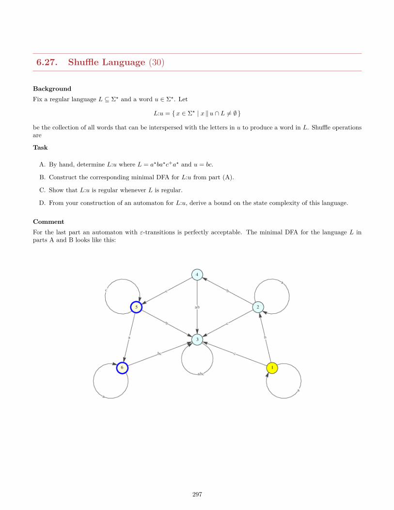
6.27. Shuffle Language (30)

BackgroundFix a regular language L ⊆ Σ? and a word u ∈ Σ?. Let

L:u = x ∈ Σ? | x ‖u ∩ L 6= ∅

be the collection of all words that can be interspersed with the letters in u to produce a word in L. Shuffle operationsare

Task

A. By hand, determine L:u where L = a?ba?c+a? and u = bc.

B. Construct the corresponding minimal DFA for L:u from part (A).

C. Show that L:u is regular whenever L is regular.

D. From your construction of an automaton for L:u, derive a bound on the state complexity of this language.

CommentFor the last part an automaton with ε-transitions is perfectly acceptable. The minimal DFA for the language L inparts A and B looks like this:

297

6.28. Frontiers (50)

BackgroundRecall that a language is prefix if no word is a prefix of another word in the language. There is a close connectionbetween prefix sets and prefix-closed sets. To see this, define the proper prefixes and the frontier of a language L ⊆ Σ?as follows.

pp(L) = Σ? − L · Σ?

fr(L) = L · Σ− L

Clearly, pp(L) is prefix-closed and fr(L) is prefix. L ⊆ Σ+ is right complete if for any word w there exists a wordu ∈ L such that wΣ? ∩ uΣ? 6= ∅.

Task

A. Show that pp(fr(C)) = C whenever C ⊆ Σ? is prefix-closed.

B. Show that fr(pp(P )) = P whenever P ⊆ Σ? is prefix.

C. Show that L is a frontier language if every for every word w there is some x ∈ L such that w ≤ x or x < w.

CommentFrontier languages are useful in constructing DFAs for regular languages by unfolding the minimal DFA.

298

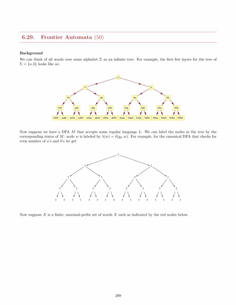
6.29. Frontier Automata (50)

BackgroundWe can think of all words over some alphabet Σ as an infinite tree. For example, the first few layers for the tree ofΣ = a, b looks like so:

Now suppose we have a DFA M that accepts some regular language L. We can label the nodes in the tree by thecorresponding states of M : node w is labeled by λ(w) = δ(q0, w). For example, for the canonical DFA that checks foreven number of a’s and b’s we get

Now suppose X is a finite, maximal-prefix set of words X such as indicated by the red nodes below.

299

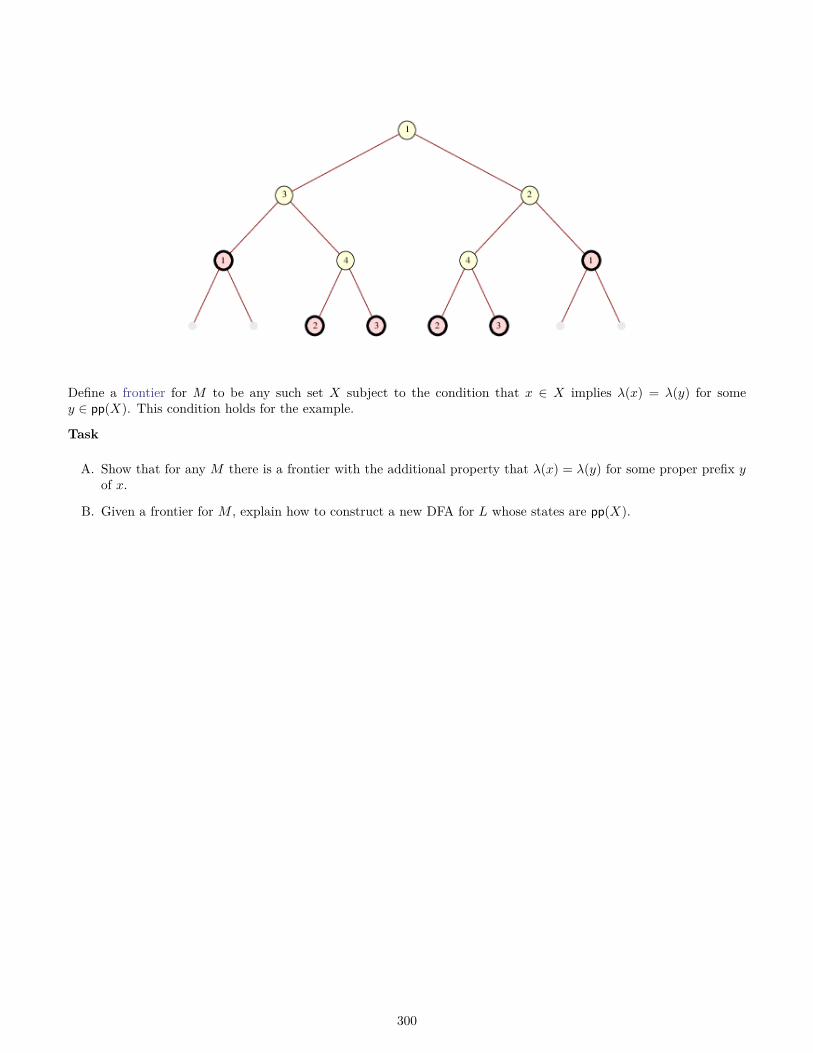
Define a frontier for M to be any such set X subject to the condition that x ∈ X implies λ(x) = λ(y) for somey ∈ pp(X). This condition holds for the example.

Task

A. Show that for any M there is a frontier with the additional property that λ(x) = λ(y) for some proper prefix yof x.

B. Given a frontier for M , explain how to construct a new DFA for L whose states are pp(X).

300

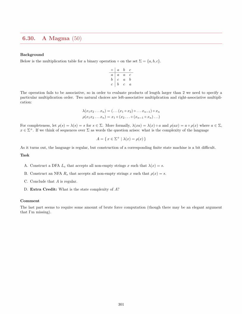
6.30. A Magma (50)

BackgroundBelow is the multiplication table for a binary operation on the set Σ = a, b, c.

a b ca a a cb c a bc b c a

The operation fails to be associative, so in order to evaluate products of length larger than 2 we need to specify aparticular multiplication order. Two natural choices are left-associative multiplication and right-associative multipli-cation:

λ(x1x2 . . . xn) = (. . . (x1 x2) . . . xn−1) xnρ(x1x2 . . . xn) = x1 (x2 . . . (xn−1 xn) . . .)

For completeness, let ρ(s) = λ(s) = s for s ∈ Σ. More formally, λ(xa) = λ(x) a and ρ(ax) = a ρ(x) where a ∈ Σ,x ∈ Σ+. If we think of sequences over Σ as words the question arises: what is the complexity of the language

A = x ∈ Σ+ | λ(x) = ρ(x)

As it turns out, the language is regular, but construction of a corresponding finite state machine is a bit difficult.

Task

A. Construct a DFA Ls that accepts all non-empty strings x such that λ(x) = s.

B. Construct an NFA Rs that accepts all non-empty strings x such that ρ(x) = s.

C. Conclude that A is regular.

D. Extra Credit: What is the state complexity of A?

CommentThe last part seems to require some amount of brute force computation (though there may be an elegant argumentthat I’m missing).

301

6.31. A Quadratic Language Equation (50)

BackgroundWe have seen that certain linear equations for languages can be solved (Arden’s Lemma). In general, though, evensimple equations for languages are rather difficult to deal with. For example, consider the problem of solving

L · L = Σ?

A trivial solution is L = Σ?, but how about other solutions? For simplicity consider only the alphabet a, b.

Task

A. Verify that L = ε+ aΣ? + Σ?b is a solution.

B. The state complexity of the last solution is 4. Find a solution of state complexity 3.

C. Find another solution of state complexity 3 that cannot be obtained from the previous one by swapping a and b.

CommentThere are 92 solutions of state complexity 3, so there is quite a bit of choice. Think about excluded words.

302

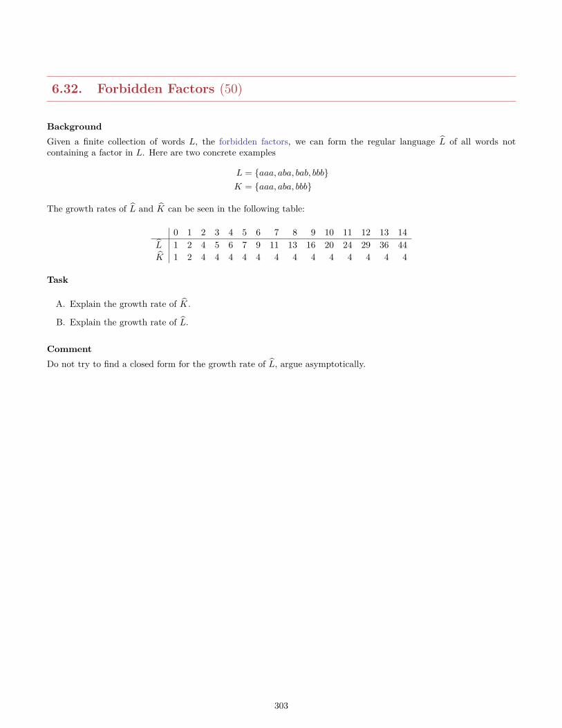
6.32. Forbidden Factors (50)

BackgroundGiven a finite collection of words L, the forbidden factors, we can form the regular language L of all words notcontaining a factor in L. Here are two concrete examples

L = aaa, aba, bab, bbbK = aaa, aba, bbb

The growth rates of L and K can be seen in the following table:

0 1 2 3 4 5 6 7 8 9 10 11 12 13 14L 1 2 4 5 6 7 9 11 13 16 20 24 29 36 44K 1 2 4 4 4 4 4 4 4 4 4 4 4 4 4

Task

A. Explain the growth rate of K.

B. Explain the growth rate of L.

CommentDo not try to find a closed form for the growth rate of L, argue asymptotically.

303

6.33. Subwords and Halfs (50)

BackgroundWrite sw`(x) for the collection of all factors of x of length `. Thus, sw`(x) has cardinality |x| − ` + 1 for all words xof length at least `, and 0 otherwise.

Task

A. Let K ⊆ Σ≤` be a finite language. Construct a DFA for the language

L`,K = x ∈ Σ? | ∀u ∈ sw`(x)(u ∈ Σ?KΣ?)

B. Let L be any regular language. Construct a finite state machine for the language

L1/2 = x ∈ Σ? | ∃ y ∈ Σ? (xy ∈ L ∧ |x| = |y|)

C. How aboutLrep = zz ∈ Σ? | z ∈ Σ?

304

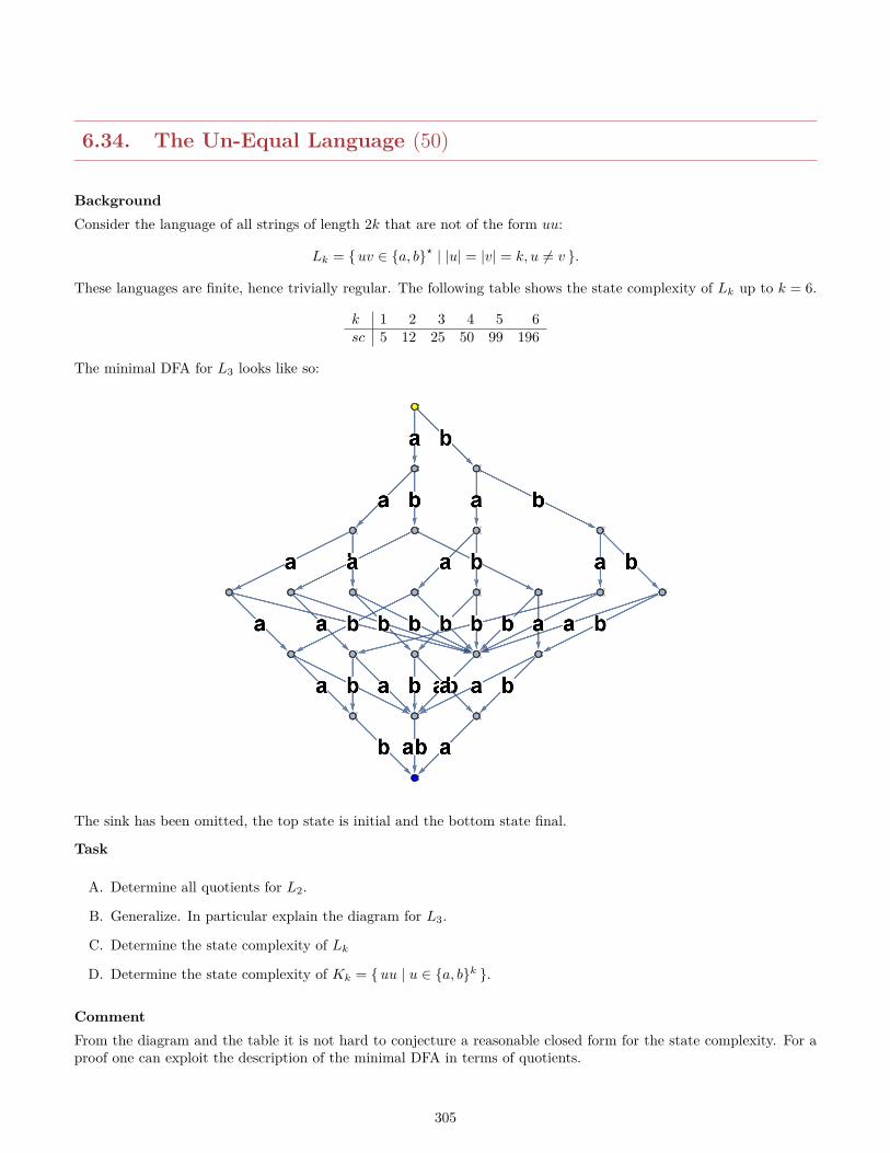
6.34. The Un-Equal Language (50)

BackgroundConsider the language of all strings of length 2k that are not of the form uu:

Lk = uv ∈ a, b? | |u| = |v| = k, u 6= v .

These languages are finite, hence trivially regular. The following table shows the state complexity of Lk up to k = 6.

k 1 2 3 4 5 6sc 5 12 25 50 99 196

The minimal DFA for L3 looks like so:

The sink has been omitted, the top state is initial and the bottom state final.

Task

A. Determine all quotients for L2.

B. Generalize. In particular explain the diagram for L3.

C. Determine the state complexity of Lk

D. Determine the state complexity of Kk = uu | u ∈ a, bk .

CommentFrom the diagram and the table it is not hard to conjecture a reasonable closed form for the state complexity. For aproof one can exploit the description of the minimal DFA in terms of quotients.

305

6.35. MSO and Regular Languages (25)

BackgroundAccording to Buchi’s theorem, monadic second-order logic defines exactly the regular languages. However, we gave noproof for the direction “MSO implies regular.” Here goes. We are trying to show that for every sentence ϕ in MSO[<]the associated language

L(ϕ) = w ∈ Σ? | w |= ϕ

is in fact regular. The proof uses induction on the buildup of ϕ. Alas, there is the usual problem with semantics:the components of a sentence typically contain free variables, they are not sentences themselves. To deal with freevariables it is best to consider augmented words over the alphabet

Γ = Σ× (2)k

where k is the number of variables, both first-order and second-order. In other words, we add an appropriate numberof binary tracks to the original word that can be used to interpret the free variables in the quantifier-free part. Thereis no need for padding, the additional tracks have the same length as w. This is essentially the same machinery as formonadic second-order logic on infinite words discussed in class.Also recall our formula even(X) for “X has even cardinality” from class.

Task

A. Prove by induction on the buildup of ϕ that L(ϕ) is regular. You may safely assume that the formula is inprenex normal form.

B. What can you say about the state-complexity of L(ϕ)? Specifically, how large is the machine for the quantifier-free part and what happens when you deal with the quantifiers?

C. Translating even(X) into a FSM following your inductive definition and the formula from class would produce alarge and ugly machine. Construct a small machine directly for this formula.

CommentFor part (B) don’t try to get precise results, just a rough estimate of a how large these machines could be comparedto the size of the formula. Part (C) is important: sometimes one can streamline machines quite a bit compared to thecookie-cutter result from the algorithm. In particular it may be helpful to enlarge the language by certain predicateswith pre-defined machines.

306

6.36. Representations of Regular Languages (50)

Background

TaskWe have seen that a regular language (i.e., a language that is accepted by a finite state machine) can also be describedby a regular expression or by a formula in MSO[<].Recall that u is a factor of v if ∃x, y ∈ Σ? (v = xuy) and u = u1u2 . . . un is a subword of v if ∃x0, . . . , xn ∈ Σ? (v =x0u1x1u2x3 . . . unxn).Let K be the language of all words over alphabet Σ = a, b, c containing exactly two factors ab. Likewise, let L bethe language of all words over alphabet Σ = a, b, c containing exactly two subwords ab.

A. Construct the minimal automaton for K and L.

B. Give a regular expression for K and L.

C. Give a formula in MSO[<] for K and L.

CommentFor the regular expressions and formulae try to find short, elegant answers.

307

6.37. Primitivity and Minimality (30)

BackgroundLet w be an non-empty word. Then z is the root of w if w ∈ z? but there is no shorter word with this property. Aword is primitive if it is its own root. For example, ab is the root of abababab. The primitive words of length 3 overa, b are aab, aba, abb, baa, bab, bba.Given a binary word u = u0u1 . . . un−1 define the corresponding subset of S(u) ⊆ 0, 1, . . . , n − 1 by i ∈ S(u) ⇐⇒ui = 1 (in other words, think of u as a bitvector for membership). Define a DFA M(u) over the one-letter alphabeta as follows:

M(u) = 〈0, 1, . . . , n− 1, a, δ; 0, S(u)〉

where n = |u| and δ(p, a) = p+ 1 mod n.

Task

A. Show that M(u) is minimal if, and only if, u is primitive (reason about the behavior of the states in M(u)).

B. Give an alternative proof by “running” a minimization algorithm on M(u).

C. Find a way to characterize minimal DFAs over a one-letter alphabet.

CommentFor the last part come up with an elegant description of the automata and make sure to prove that your descriptionis correct.If you like extra work (for extra credit), figure out how to count minimal DFAs of size n over a one-letter alphabet.

308

6.38. Definite Automata (50)

BackgroundFinite state machines are often called memoryless devices since they do not have access to any kind of RAM memory.On the other hand, even a DFA can remember certain inputs unboundedly long. Here is a type of finite state machinethat truly forgets.An accessible DFA is definite if for some r ≥ 0, all words of length at least r and all states p and q: δ(p, x) = δ(q, x). Ifr is minimal with this property, the DFA is said to be r-definite. Thus, in a definite DFA, acceptance of a sufficientlylong input depends solely on the suffix of length r of the input. A regular language is definite if it can be accepted bya definite DFA.

Task

A. Show that La,−3, the language of all words with an a in position −3, is definite.

B. Let A ⊆ Σ? be any finite language. Show that Σ?A is definite.

C. Develop an algorithm that tests if a DFA is definite, and computes r, if it exists. Make sure to explain why youralgorithm is correct.

D. What is the complexity of your algorithm?

Comment

309

6.39. Right Quotients (25)

BackgroundLeft quotients are defined by removing a prefix from a word. Needless to say, we can also define right quotients byremoving a suffix:

L/x = y ∈ Σ? | yx ∈ L

Algebraically, these right quotients behave very much like their left cousins.Left quotients are directly related to behaviors and can be used to decompose a regular language; one might wonderif regular languages can also be described in some interesting way in terms of right quotients. The answer is yes, butthings become a bit more complicated.In the following, assume M = 〈Q,Σ, δ; q0, F 〉 is the minimal DFA accepting some language L. Fix some state p and,for all states q 6= p, choose a witness wq ∈ Σ? such that δ(p, wq) ∈ F ⇐⇒ δ(q, wq) /∈ F (which witness exists since Mis minimal).

Task

A. Show that for any Boolean operation ⊕ we have (L⊕K)/x = L/x⊕K/x.

B. Let K ⊆ L be the language accepted by the automaton 〈Q,Σ, δ; q0, p〉. Show that K =⋂q 6=pRq where

Rq = L/wq whenever δ(p, wq) ∈ F , and Rq = Σ? − L/wq when δ(p, wq) /∈ F .

C. Correspondingly, write L as a Boolean combination of right quotients of L.

310

6.40. Direct Languages (50)

BackgroundA DFA is direct if it has at most one final state. A regular language is direct if it is accepted by some direct DFA.Note the restriction to DFAs; the language a, aa for example fails to be direct.

Task

A. Find a regular language L such that L− F fails to be direct for any finite language F .

B. Explain the connection between direct languages and prefix languages.

Comment

311

6.41. Prefix Languages (50)

BackgroundA language is prefix if no word in the language is a proper prefix of another word in the language. Some would arguethat these languages should be called prefix-free, but why should terminology yield to logic?

Task

A. Given an algorithm that decides whether the language accepted by a DFA is prefix.

B. What is the running time of your algorithm?

Comment

312

6.42. Recognizing Suffixes (20)

BackgroundA DFA has no a priori information about the length of an input string. For example, it does not know when it scansthe third symbol from the end (as opposed to the third symbol from the start). As a result, it is quite difficult toconstruct DFAs that recognize languages based on conditions of some suffix of the input.For any integer k 6= 0 write

La,k = x ∈ a, b? | xk = a

For negative k this is interpreted as “kth symbol from the back”. For example,

La,2 = aa, ba, aaa, aab, baa, bab, . . .La,−3 = aaa, aab, aba, abb, aaaa, aaab, . . .

Task

A. Show how to construct a DFA that accepts La,k for positive k.

B. Show how to construct a DFA that accepts La,k for negative k.

Part 1 is easy, but part 2 requires some work. Try to find an elegant description of these machines.

313

6.43. Local Languages (50)

BackgroundRegular languages can be construed as homomorphic images of certain particularly simple regular languages, socalled local languages. A Σ-language L is local if there are sets A,B ⊆ Σ and a binary relation R on Σ such thatL(A,B,R) = x1x2 . . . xn | x1 ∈ A, xn ∈ B, R(xi, xi+1) . For example, let Σ = a, b, c, d be an ordered alphabetwith order relation < as indicated. Then L(a, d, <) = a+b?c?d+, L(a, a, <) = a+ and L(d, a, <) = ∅.

Task

A. Show that every local language is regular.

B. Show that every regular language is a homomorphic image of a local language.

Comment

314

6.44. Dihedral Recognizer (50)

BackgroundConsider the dihedral group D4 with generators a and b where a2 = b4 = 1 and ba = a3b. The group has 8 elementsand can be written as 1, a, a2, a3, b, ba, ba2, ba3. Here a corresponds to a rotation by 90 degrees, and b is the reflectionalong the horizontal axis.If we think of a and b as symbols over a two-letter alphabet words over this alphabet naturally correspond to groupelements. More precisely, there is an evaluation map η : Σ? → D4 which turns out to be a monoid homomorphism.

Task

A. Explain the group elements 1, a, a2, a3, b, ba, ba2, ba3 geometrically.

B. Show that the language L ⊆ Σ? of all words that evaluate to 1 is regular. Construct the minimal DFA for L.

C. Determine the cardinality of L ∩ Σn.

Comment

315

6.45. Recognizing Permutations (50)

BackgroundMachines for finite languages are special in many ways; there are special algorithms for their construction and manytasks are computationally easier than in the general case. Still, it can be challenging to construct the minimal DFAfor a finite language. Here is an example: we can think of a permutation of length k as a word of length k over ak-letter alphabet. E.g., all permutations of length 3 are given by the finite language

S3 = abc, acb, bac, bca, cab, cba

Recall that the alternating group is the subgroup of the full symmetric group on k letters containing all permutationsthat can be written as the product of an even number of transpositions. For k = 4 we obtain

E4 = abcd, acdb, adbc, badc, bcad, bdca, cabd, cbda, cdab, dacb, dbac, dcba

We write Sk for the full symmetric group on k letters and Ak for the alternating subgroup; Sk and Ek for thecorresponding sets of words obtained by using all permutations or just the even ones. Hence |Sk| = k! and |Ek| = k!/2.

Task

A. Determine the state complexity of Sk.

B. Determine the state complexity of Ek.

C. How about the state complexity of the set of “odd words,” Sk − Ek?

CommentUnless you have perfect intuition, you will need to compute some of these state complexities by brute force to get anidea of what is going on. Specifically, you can run the quotient machine construction on Pk and Ek and then observehow the states in these machines group words together. There is a strong pattern which translates into the rightcounting functions. The solution for the alternating group requires special cases for k = 1, 2; everything is uniform fork ≥ 3. The languages Ek for k ≤ 7 are at http://www.cs.cmu.edu/˜flac/AlternatingWords.txt

Check the wikipedia or some algebra text if you feel uneasy about the alternating group.

316

6.46. Balance and Majority (20)

BackgroundWrite |x|0 for the number of 0’s in a binary word x, and likewise |x|1 for the number of 1’s. The balance languageLbal is the set of all binary words that have the same number of 1’s and 0’s:

Lbal = x ∈ 2? | |x|1 = |x|0 .

The majority language Lmaj is the set of all binary words that have at least as many 1’s as 0’s:

Lmaj = x ∈ 2? | |x|1 ≥ |x|0 .

Task

A. Show that there is no finite state machine that accepts Lbal.

B. Show that there is no finite state machine that accepts Lmaj.

CommentThe essential issue is that in order to recognize these languages a DFA would require some kind of unbounded countingability – and DFAs can only count in a bounded way. Try to come up with a clean, concise argument. Also note thatyour argument has to cover all possible finite state machines, you cannot make any assumptions about, say, the sizeof the machine.

317

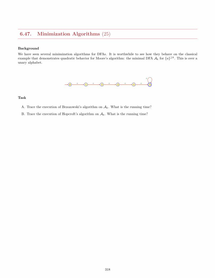
6.47. Minimization Algorithms (25)

BackgroundWe have seen several minimization algorithms for DFAs. It is worthwhile to see how they behave on the classicalexample that demonstrates quadratic behavior for Moore’s algorithm: the minimal DFA Ak for a≥k. This is over aunary alphabet.

0 1 2 3 4 5a a a a a

a

Task

A. Trace the execution of Brzozowski’s algorithm on Ak. What is the running time?

B. Trace the execution of Hopcroft’s algorithm on Ak. What is the running time?

318

6.48. State Merging (50)

BackgroundBelow is the transition matrix for a 15-state DFA M over the alphabet a, b. Initial state is 1 and the final statesare 8, 9, 10, 11.

1 2 3 4 5 6 7 8 9 10 11 12 13 14 15a 2 4 6 8 10 12 14 8 10 12 14 8 10 12 14b 3 5 7 9 11 13 15 9 11 13 15 9 11 13 15

The machine M turns out to be non-minimal.

Task

A. Use the state merging algorithm to compute the minimal DFA for this machine.

B. What is the language accepted by the machine? Give a short, clear description.

C. Try to generalize: the language of M is just one example of a class of languages Lk, k ≥ 1. What do the minimalautomata look like in general? In particular, pin down the state complexity of these languages.

CommentMake sure to build a nice table for the state merging process, don’t just write down the final result. If you like, youcan write a program to do this or use my code on the web. It’s a good idea, though, to run the algorithm by hand acouple of times, just to get the hang of it.For part C it’s a good idea to draw a nice picture of the minimal automaton for M .

319

6.49. Minimal Automata for Finite Languages (50)

BackgroundBrute-force construction of DFAs often lead to machines that are far from minimal. One such example is the applicationof the product machine construction to obtain a DFA for a finite language such as

L = ba, bb, aaa, aab ⊆ a, b?

Task

A. Construct the accessible part of the brute-force product machine for L, built from the natural DFAs Mw forw ∈ L.

B. Construct the minimal DFA for L directly by hand, making sure not to introduce any unnecessary states. Youmight wish to identify the states with prefixes of the words in L.

C. Use the minimization algorithm from class to check that your product machine after state-merging produces thesame (really: isomorphic) automaton as in part 2.

D. In a practical algorithm one would not necessarily represent the transition function of the DFA by a two-dimensional lookup table or hashtable. What other data structure lends itself naturally to implement an DFAfor a finite language? Explain your choice.

CommentIf you have problems with the construction in part 2, start with a language with just 2 words and figure out how tobuild the minimal DFA in that case.

320

6.50. Fast Equivalence Testing (20)

BackgroundIn class we gave an algorithm to test whether two DFAs M1 and M2 are equivalent that uses the Union/Find data-structure to maintain an equivalence relation E on Q = Q1 ∪ Q2. The algorithm avoids minimization and runs inessentially linear time.For this problem consider the following two machines, both over alphabet a, b. M1 has 4 states, initial state 1 andfinal states 3, 4. The transition matrix is

1 2 3 4a 2 3 3 2b 1 4 4 1

M2 has 7 states, initial state 1 and final states 4, 5. The transition matrix is

1 2 3 4 5 6 7a 2 4 6 4 6 4 6b 3 5 7 5 7 5 7

Make sure to renumber the states in M2 to 5, 6, . . . , 11 to make the state sets disjoint.

Task

A. As an example, compute the equivalence relation E for the two machines from above. Are they equivalent?

B. Prove that the algorithm is correct in general. To this end it’s probably a good idea to show that δ(q01, x) Eδ(q02, x) for all words x.

Needless to say you, don’t have to use the Union/Find method in your hand calculation. It is much easier to maintaina list of blocks.

321

6.51. Counting Minimal Tally DFAs (50)

BackgroundIt is rather difficult to determine the number of (n, k)-DFAs that are minimal (up to isomorphism). However, the inspecial case where k = 1 things are manageable. The following table shows the number of minimal (n, 1)-DFAs up ton = 12.

n 1 2 3 4 5 6 7 8 9 10 11 12# 2 4 12 30 78 180 432 978 2220 4926 10908 23790

Task

A. Find a way to count the number of minimal (n, 1)-DFAs.

B. Generate all minimal (6, 1)-DFAs and explain their acceptance languages.

CommentTry to exploit part (A) for part (B); your method should work in practice for n = 10 as well. Brute force is not agood idea.

322

6.52. Divisibility (40)

BackgroundNumbers written in base B ≥ 2 can be construed as words over a digit alphabet D = 0, 1, . . . , B − 1. We canassociate a numerical value to such a string via

val(x1x2 . . . xn) =n∑i=1

Bn−ixi

This corresponds to the MSD being first in the string (a really bad idea, but standard notation). Alternatively, wecan place the MSD at the end:

valR(x1x2 . . . xn) =n∑i=1

Bi−1xi

This is referred to as reverse base-B notation.Now suppose we have a number given in either base-B or reverse base-B notation. We would like to test whether thenumber is divisible by some modulus m ≥ 1.

Task

A. Construct a DFA that accepts x iff val(x) = 0 (mod m).

B. Construct a DFA that accepts x iff valR(x) = 0 (mod m).

CommentIt is difficult to describe the state complexity of these languages, just build a natural DFA without worrying muchabout its size.

323

6.53. Divisibility In Reverse Binary (50)

BackgroundWe have seen that one can check divisibility by a fixed modulus m on a DFA regardless of the base B. More precisely,we showed how to construct a DFA for words x written in base B notation with the MSD in the first position. Ofcourse, there is no real reason why the MSD should be up front, it might as well be the last digit (reverse binarynotation).

Task

1. Construct a DFA that tests divisibility by 3 for numbers written in reverse binary. To do this, find a way toexpress ν(xa) in terms of ν(x) and |x| and choose your state set accordingly.

2. Show how to generalize this construction for arbitrary moduli and bases.

3. How does the size of your machine for m = 5 and B = 2 in reverse binary compare to the machine constructedin class for normal binary notation? What is going on?

CommentNaturally one would like to know how large the minimal automata are in general, for arbitrary base B and arbitrarymodulus m, and for ordinary base B notation as well as reverse base B. Lots of extra credit if you can give a generalcharacterization.

324

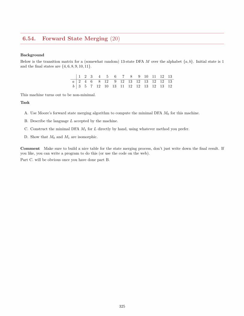
6.54. Forward State Merging (20)

BackgroundBelow is the transition matrix for a (somewhat random) 13-state DFA M over the alphabet a, b. Initial state is 1and the final states are 4, 6, 8, 9, 10, 11.

1 2 3 4 5 6 7 8 9 10 11 12 13a 2 4 6 8 12 9 12 13 12 13 12 12 13b 3 5 7 12 10 13 11 12 12 13 12 13 12

This machine turns out to be non-minimal.

Task

A. Use Moore’s forward state merging algorithm to compute the minimal DFA M0 for this machine.

B. Describe the language L accepted by the machine.

C. Construct the minimal DFA M1 for L directly by hand, using whatever method you prefer.

D. Show that M0 and M1 are isomorphic.

Comment Make sure to build a nice table for the state merging process, don’t just write down the final result. Ifyou like, you can write a program to do this (or use the code on the web).Part C. will be obvious once you have done part B.

325

6.55. More Forward State Merging (20)

BackgroundWe have seen that the standard forward state merging algorithm can be implemented in expected time O(n2) (assumingthe alphabet has fixed size). However, often the running time is better than quadratic since the number of refinementsteps

ηk+1 = ηk u ηa1k u η

a2k u . . . u η

ank

is far less than n.

Task

A. Give an example of a machine with n states where n− 2 refinement steps are required before the approximationprocess stops.

B. The standard implementation uses a hash table in the refinement step, so in principle the running time could beworse than quadratic (however unlikely such a failure may be). Give a modified version of the algorithm that isguaranteed quadratic time.Hint: get rid of the hash tables and use a lookup table instead.

326

6.56. Determinization (50)

BackgroundWe have seen that nondeterministic machines are often much easier to construct for given languages than theirdeterministic counterparts. Here are two such examples.

A = w,w′B = x ∈ a, b? | x−k = a

Here w and w′ are arbitrary distinct words over a, b.

Task

A. Explain what the natural NFA (no ε-moves) for A looks like. What is the state complexity?

B. Determine the DFA M obtained from this machine by applying the power automaton construction (accessiblepart only). Give a bound on the state complexity.

C. Should one expect the machine M to be minimal? Explain.

D. Repeat for the language B.

327

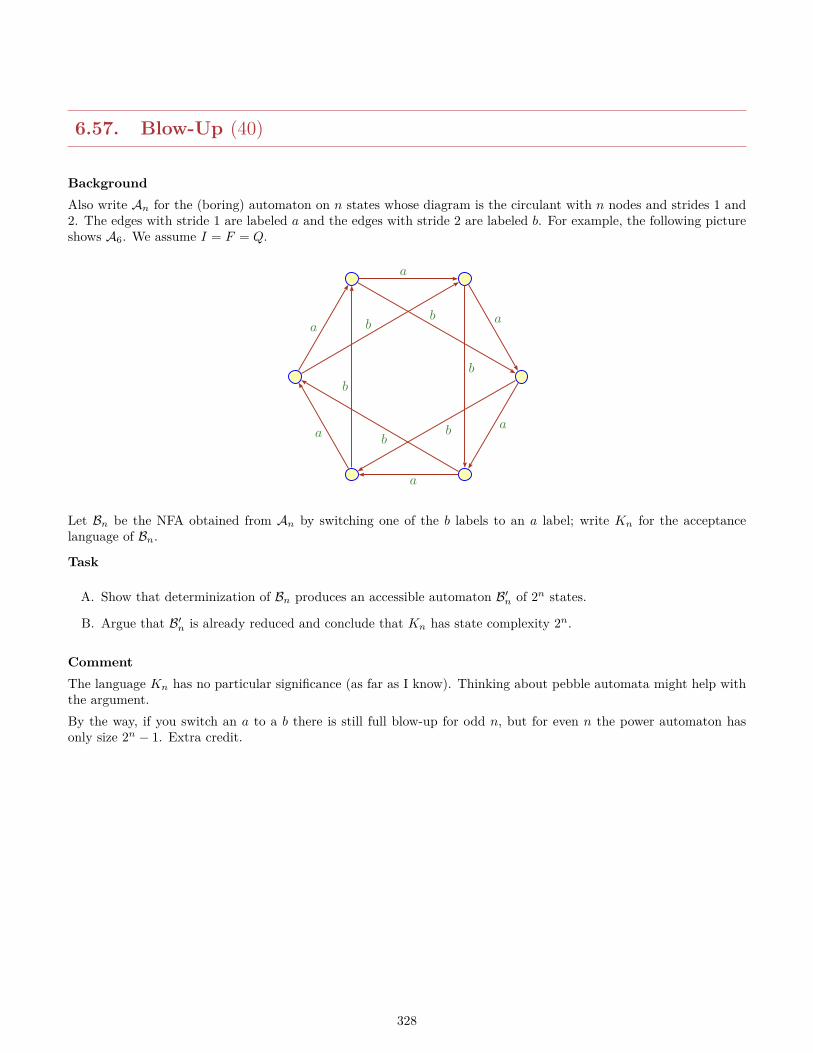
6.57. Blow-Up (40)

BackgroundAlso write An for the (boring) automaton on n states whose diagram is the circulant with n nodes and strides 1 and2. The edges with stride 1 are labeled a and the edges with stride 2 are labeled b. For example, the following pictureshows A6. We assume I = F = Q.

a

a

a

a

a

a

b

bb

b

bb

Let Bn be the NFA obtained from An by switching one of the b labels to an a label; write Kn for the acceptancelanguage of Bn.

Task

A. Show that determinization of Bn produces an accessible automaton B′n of 2n states.

B. Argue that B′n is already reduced and conclude that Kn has state complexity 2n.

CommentThe language Kn has no particular significance (as far as I know). Thinking about pebble automata might help withthe argument.By the way, if you switch an a to a b there is still full blow-up for odd n, but for even n the power automaton hasonly size 2n − 1. Extra credit.

328

6.58. Determinization and Blowup (50)

BackgroundFrom an algorithmic perspective, the Rabin-Scott powerset construction has the obvious problem of being potentiallyexponential, not just in time but even in space.

Task

A. Explain how to implement the Rabin-Scott determinization procedure, assuming an alphabet of fixed size k. Tryto make the running time is nearly linear in the size of the (accessible part of the) output machine as possible.

B. Construct a family of nondeterministic machines An on n states over a 2-symbol alphabet such that the powerautomaton of An has size 2n and is already minimal.

CommentThink about what it means for the states of a power automaton (i.e., subsets of the state set of the nondeterministicmachine) to be behaviorally inequivalent.

329

6.59. Syntactic Semigroups (30)

BackgroundThe standard measure of complexity of a regular language L is the number of states of its minimal DFA ML. Al-ternatively, we could use the cardinality of the syntactic semigroup Σ+/ ≡ of L. Here the syntactic congruence ≡ isdefined as follows:

x ≡ y ⇐⇒ ∀u, v ∈ Σ? (uxv ∈ L ⇔ uyv ∈ L)

Computing the syntactic semigroup according to this definition is often quite tedious, it is usually best to try todetermine the equivalence classes (first [a], then [b], then [ab], and so on). Fortunately, there is a better way: thesyntactic semigroup is isomorphic to the transition semigroup δx | x ∈ Σ+ . Thus, we can compute it using a simpleclosure operation applied to δa, a ∈ Σ.

Task

A. Compute the syntactic semigroup of L = aab over alphabet a, b?.

B. Compute the syntactic semigroup of L = ab? over alphabet a, b?.

C. Figure out what x ≡ y means in terms of the minimal automaton for L.

D. Conclude that the syntactic semigroup is isomorphic to the transition semigroup of the minimal automaton.

CommentIt is not a bad idea to use part (D) to check the computations in (A) and (B). You might want to write a program todo this.One can similarly consider syntactic monoids by working over Σ? rather than Σ+. Unfortunately, there is no goodway to fold both approaches into one.

330

6.60. Well-Ordered Languages (40)

BackgroundFor words x, y ∈ Σ? write x < y to indicate that x is lexicographically less than y. Consider a language L ⊆ Σ?; if〈L,<〉 is a well-order we will simply call L well-ordered and omit any reference to lexicographic ordering. For alphabetsof size larger than one, Σ? is not well-ordered:

1 > 01 > 001 > 0001 > 00001 > . . .

On the other hand, 1? 0 is easily seen to be well-ordered. We are mostly interested in the case where L is regular.For well-ordered L we write ot(L) for its order type. Recall that a language L is called prefix if no proper prefix ofany word in L is in L. Also, L ⊆ 2? is called complete prefix if it is prefix and for any prefix u of a word in L we have:u0 is a prefix of L iff u1 is a prefix of L.

Task

A. Show that the order type of 1? 0 is ω, and the order type of 1? 0 1? is ω2.

B. Show that for any well-ordered regular language L ⊆ Σ? there exists another well-ordered regular languageL′ ⊆ 2? such that

• L′ is complete prefix over the alphabet 2, and• the ordertype of L′ is the same as the ordertype of L.

C. Explain how to compute in polynomial time a DFA for L′ given a DFA for L.

CommentOrder type ω2 means that you have ω many copies of ω, something like

1 < 3 < 5 < . . . < 2 < 6 < 10 < . . . < 4 < 12 < 20 < . . . < 2k < 3 · 2k < 5 · 2k . . .

For the second part break things up into several steps: prefix, binary and lastly complete (while always preservingordertype).Also, this is the tip of an iceberg: we will consider structures that are defined by finite state machines in some detaillater.

Extra Credit: Figure out which order types can be realized this way. This is hard.

331

6.61. The Dyck Language (50)

BackgroundHere is a formal description (actually, several) of the language of all balanced strings of parentheses, the so-calledDyck language D. Thus, [ [ ] [ ] ] [ ] is a string in D but [ [ ] and ] [ are not. Less informally, we can define D by aclosure condition as follows. D is the least collection L of strings over alphabet Σ = [ , ] that

• L contains ε,

• whenever x, y are in L so is [ x ] and xy.

Here is an alternative definition of D First define a binary relation ρ on Σ? as follows.

x ρ y ⇐⇒ ∃u, v ∈ Σ? (x = u[ ] v ∧ y = uv).

Let ρ? be the transitive, reflexive closure of ρ. Yet another approach to D is in terms of a bookkeeping function. Letus define a map f : Σ? → Z by

f(x) = |x| ] − |x| [ .

Task

A. Show that repeated removal of adjacent pairs of matching parens leads to the empty string: D = x ∈ Σ? | xρ?ε .

B. Show that x ∈ D ⇐⇒ f(x) = 0 ∧ ∀ z ∈ Pref(x) (f(z) ≥ 0)

CommentYou should think about generalizations to languages involving several types of parens.

332

6.62. Pumping (50)

BackgroundCall a language L pumpable if there exists a number N (which depends solely on L) such that for all words w in Lwith |w| ≥ N , there exist words x, y and z such that:

• w = xyz, |xy| ≤ N and y 6= ε,

• for all t ≥ 0: xytz ∈ L.

The famous Pumping Lemma can then be stated like so: Every regular language is pumpable.

Task

A. Use the Pumping Lemma to show that the following languages are not regular.

L1 = aibi | i ≥ 0 L2 = x ∈ a, b∗ | |x|a = |x|b L3 = 02i13i | i ≥ 0

B. Show that the following language is pumpable but fails to be regular:

L = x ∈ a, b? | x contains a subword b2 or |x|b is a square .

Comment

333

6.63. DFAs versus Regular Expressions (50)

BackgroundRegular expressions are the preferred representation for regular languages in many interactive applications. Forexample, text editors such as emacs use regular expressions for search and replace operations. Clearly, it would beunreasonable to expect the user to type in a corresponding finite state machine in this case. Alas, sometimes machines,even deterministic ones, are a better representation.In the following, let Lee be the language of all strings over a, b that have an even number of a’s and an even numberof b’s. Likewise, let Loo be the odd/odd language.

Task

A. Construct the minimal DFAs for Lee and Loo.

B. Give a reasonably simple regular expression for Lee.

C. Give a regular expression for Loo.

CommentThe second part is not too bad, but the third is already a bit messy. Never mind the obvious generalizations.

334

6.64. Hard Regular Expressions (50)

BackgroundEvery regular expression corresponds to a DFA and conversely. However, there is no simple relationship between thesizes of the automata and the regular expressions.For the following problem, define

Li,j = x ∈ a, b? | |x|a = i (mod 2), |x|b = j (mod 2)

The minimal DFA for these languages is trivial:

Task

A. Find a regular expression for L00.

B. Find a regular expression for L11.

C. Find a regular expression for L01.

CommentYou must explain why your expressions are correct.

335

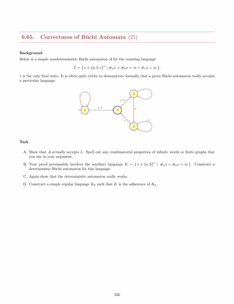
6.65. Correctness of Buchi Automata (25)

BackgroundBelow is a simple nondeterministic Buchi automaton A for the counting language

L = x ∈ a, b, cω | #ax = #bx =∞∧#cx <∞.

1 is the only final state. It is often quite tricky to demonstrate formally that a given Buchi automaton really acceptsa particular language.

0 1

2

3

a, b

a, b

a

b

b, c

b

a

Task

A. Show that A actually accepts L. Spell out any combinatorial properties of infinite words or finite graphs thatyou use in your argument.

B. Your proof presumably involves the auxiliary language K = x ∈ a, bω | #ax = #bx =∞. Construct adeterministic Buchi automaton for this language.

C. Again show that the deterministic automaton really works.

D. Construct a simple regular language K0 such that K is the adherence of K0.

336

6.66. Acceptance for Buchi Automata (25)

BackgroundWe have seen that acceptance of a Buchi automaton is undecidable if we consider sufficiently complicated input words(e.g., words specified by a computable function). However, for sufficiently simple words acceptance is still decidable.Let A = 〈Q,Σ, τ ; I, F 〉 be a Buchi automaton.

Task

A. Show how to decide whether A accepts a “constant” input word U = aω where a ∈ Σ.

B. Generalize to periodic inputs U = uω where u ∈ Σ+.

C. Generalize to ultimately periodic inputs U = vuω where u, v ∈ Σ+.

D. What is the running time of your three algorithms?

Extra Credit: Define the infinite binary word U as U(k) = 1 iff k is prime. Is it decidable whether a given Buchiautomaton accepts U? For what it’s worth, here are the first few bits of U :

U = 0011010100010100010100010000010100000100010100010000010000010 . . .

337

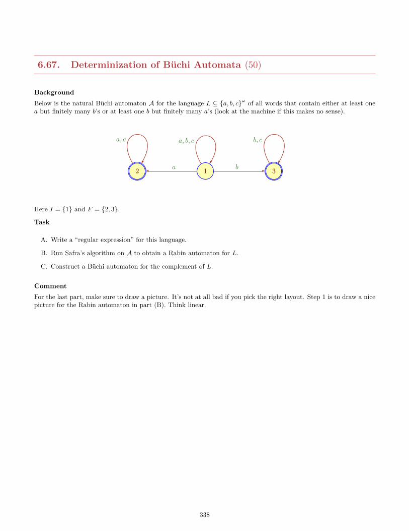
6.67. Determinization of Buchi Automata (50)

BackgroundBelow is the natural Buchi automaton A for the language L ⊆ a, b, cω of all words that contain either at least onea but finitely many b’s or at least one b but finitely many a’s (look at the machine if this makes no sense).

2 1 3a b

a, c a, b, c b, c

Here I = 1 and F = 2, 3.

Task

A. Write a “regular expression” for this language.

B. Run Safra’s algorithm on A to obtain a Rabin automaton for L.

C. Construct a Buchi automaton for the complement of L.

CommentFor the last part, make sure to draw a picture. It’s not at all bad if you pick the right layout. Step 1 is to draw a nicepicture for the Rabin automaton in part (B). Think linear.

338

6.68. Parikh Languages (30)

BackgroundOne can simplify formal languages by pretending that letters commute: ab = ba and so forth, so we can replace aword by its sorted version. More precisely, the commutative image or Parikh language of L ⊆ Σk?, Σk = a1, . . . , akis defined by

L# = ae11 . . . aenn | ∃x ∈ L (ei = |x|ai , i = 1, . . . , k ) .

The counting languages Ck ⊆ Σk? are defined by C#k = ai1ai2 . . . aik | i ≥ 1 .

Task

A. Construct a context-sensitive grammar for the language C4. Conclude that all the languages Ck are context-sensitive.

B. Show that the Parikh language L# is context sensitive whenever L is context sensitive.

C. Show that Ck is context-free iff k ≤ 2.

D. Show that there exists a regular language R such that R# is not context-free.

339

6.69. Solving Language Equations (50)

Background

Task

A. What language is described by the system X = aXb+XX + ε?

B. Use Arden’s Lemma to solve the system obtained from the minimal automaton for the language “even a’s, evenb’s.”

Comment

340

6.70. Multiplicity (50)

Background

TaskMultiplicity

A. Construct an NFA that accepts a word x ∈ a, b+ in exactly |x|b many ways.

B. Construct an NFA that accepts a word x ∈ 2+ in exactly val(x) many ways (assuming standard binary repre-sentation, MSD is first).

Comment

341

6.71. Small NFAs (50)

BackgroundLet L ⊆ Σ? be a language. A fooling set for L is a list (xi, yi) of factored words i = 1, . . . , n, such that xiyi ∈ L butfor any i 6= j we have xiyj /∈ L or xjyi /∈ L.

Task

A. Let L be a regular language with a fooling set of size n. Show that any NFA accepting L must have at least nstates.

B. Let Lm = x ∈ a, b? | #ax = 0 (mod m) . Show that any NFA for L must have at least m states.

CommentNote that Lm from part (B) is trivially recognizable by a DFA of size m, so in this case nondeterminism does not help.

342

6.72. Injectivity of Transducers (50)

BackgroundFor this problem we consider Mealy machines A = 〈Q,Σ, δ〉 where δ : Q× Σ→ Σ×Q . We write p for the transductionobtained by selecting p as initial state.A is ω-injective if for all states p and all words x, y ∈ Σω: p(x) = p(y) implies x = y. For t ≥ 0, A is t-injective if forall states p and all letters a, b ∈ Σ, words x, y ∈ Σt: p(ax) = p(by) implies a = b.

Task

A. Show that every t-injective transducer is also ω-injective.

B. Use a GAN argument to show that every ω-injective transducer is also t-injective for some t.

C. Reprove the last item by giving a bound on t in terms of the state complexity of A.

Comment

343

6.73. Composition of Transductions (25)

BackgroundSuppose we have two binary relations ρ ⊆ Σ?×Γ? and σ ⊆ Γ?×∆? and consider their composition τ = ρσ ⊆ Σ?×∆?

We mentioned in class that τ is also rational, but we gave no proof. Here goes.In the following, a transducer is called alphabetic if all labels are of the form a:b where a and b are both letters. Soan alphabetic transduction must be length-preserving.

Task

A. First assume that the transducers for ρ and σ are both alphabetic. Show that their composition is also rational.

B. Generalize the argument from part (A) to work for arbitrary transducers. Make sure in particular that youconstruction works when the relations are not length-preserving.

C. What is the running time of your construction (in terms of the number of states of the given machines)?

344

6.74. Collatz and Transducers (30)

BackgroundSuppose we write positive integers in reverse binary. Define C to be the following version of the Collatz function.

C(x) =x/2 if x even,(3x+ 1)/2 otherwise.

Task

A. Show that C can be computed by a transducer (using reverse binary).

B. Translate this transducer into a highly efficient algorithm for computing C.

C. Implement your algorithm and use the program to determine the stopping times of numbers x = 2k − 1 fork = 10000, . . . , 12000.

CommentThe difference between (A) and (B) is that a vanilla implementation of a transducer slows things down too much; youneed some clever hacks to get good performance.As the result for part (C), submit a text file that contains 2001 integers, one per line. The first few entries should be86278, 86279, 86280, 86281, 86282, 86283.Extra credit for the fastest solution.

345

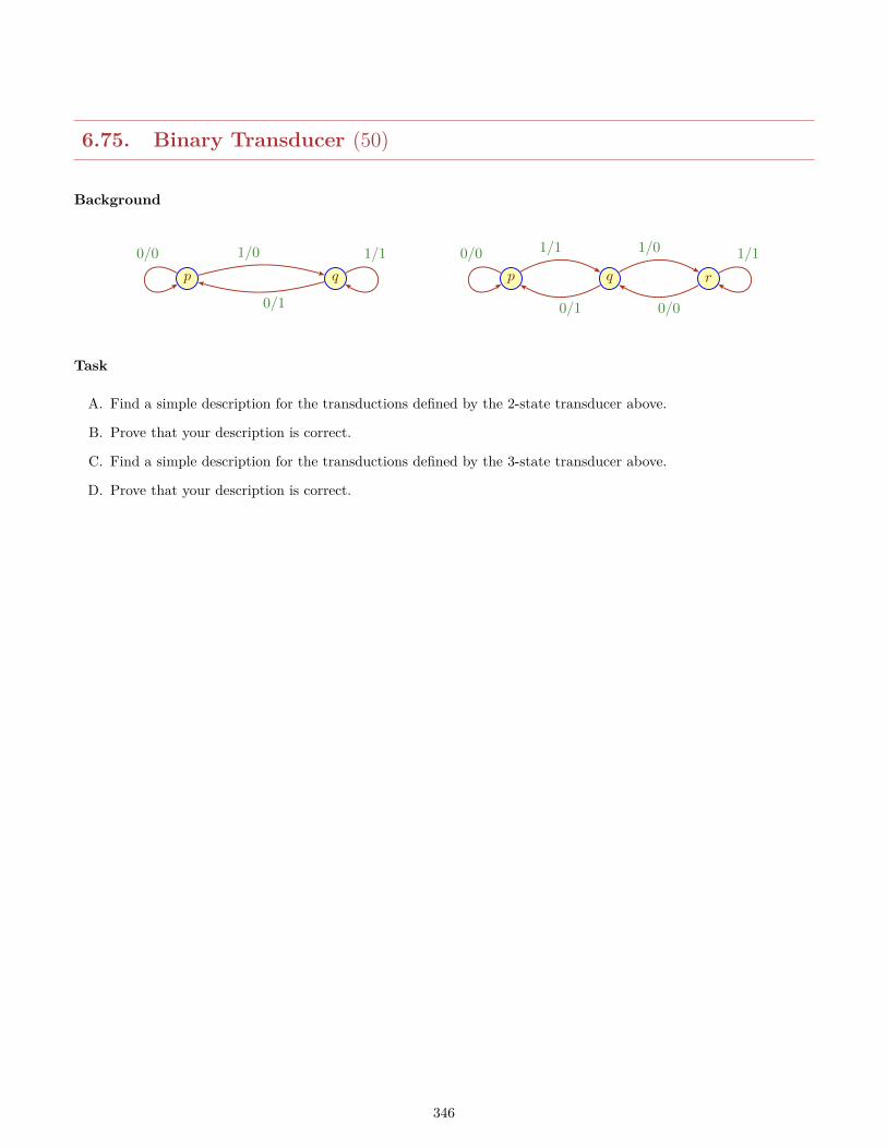
6.75. Binary Transducer (50)

Background

p q

0/0 1/0

0/1

1/1

p q r

1/1

0/1

1/0

0/0

0/0 1/1

Task

A. Find a simple description for the transductions defined by the 2-state transducer above.

B. Prove that your description is correct.

C. Find a simple description for the transductions defined by the 3-state transducer above.

D. Prove that your description is correct.

346

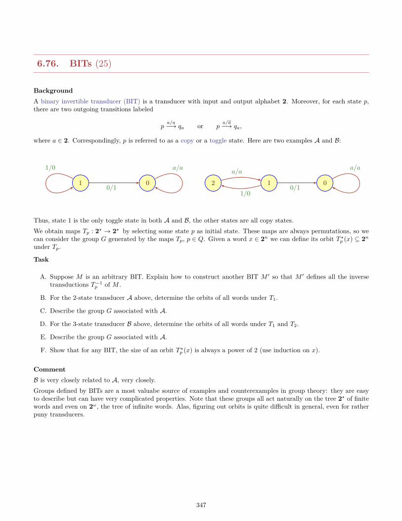
6.76. BITs (25)

BackgroundA binary invertible transducer (BIT) is a transducer with input and output alphabet 2. Moreover, for each state p,there are two outgoing transitions labeled

pa/a−→ qa or p

a/a−→ qa,

where a ∈ 2. Correspondingly, p is referred to as a copy or a toggle state. Here are two examples A and B:

1 0

1/0

0/1

a/a

2 1 0

1/0

a/a

0/1

a/a

Thus, state 1 is the only toggle state in both A and B, the other states are all copy states.We obtain maps Tp : 2? → 2? by selecting some state p as initial state. These maps are always permutations, so wecan consider the group G generated by the maps Tp, p ∈ Q. Given a word x ∈ 2n we can define its orbit T ?p (x) ⊆ 2nunder Tp.

Task

A. Suppose M is an arbitrary BIT. Explain how to construct another BIT M ′ so that M ′ defines all the inversetransductions T−1

p of M .

B. For the 2-state transducer A above, determine the orbits of all words under T1.

C. Describe the group G associated with A.

D. For the 3-state transducer B above, determine the orbits of all words under T1 and T2.

E. Describe the group G associated with A.

F. Show that for any BIT, the size of an orbit T ?p (x) is always a power of 2 (use induction on x).

CommentB is very closely related to A, very closely.Groups defined by BITs are a most valuabe source of examples and counterexamples in group theory: they are easyto describe but can have very complicated properties. Note that these groups all act naturally on the tree 2? of finitewords and even on 2ω, the tree of infinite words. Alas, figuring out orbits is quite difficult in general, even for ratherpuny transducers.

347

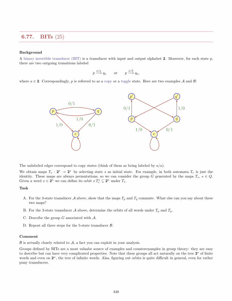
6.77. BITs (25)

BackgroundA binary invertible transducer (BIT) is a transducer with input and output alphabet 2. Moreover, for each state p,there are two outgoing transitions labeled

pa/a−→ qa or p

a/a−→ qa,

where a ∈ 2. Correspondingly, p is referred to as a copy or a toggle state. Here are two examples A and B:

e

p q

0/1

1/0

1/0 0/1

e

p q

p′ q′

0/1 1/0

1/0 0/1

The unlabeled edges correspond to copy states (think of them as being labeled by a/a).We obtain maps Ts : 2? → 2? by selecting state s as initial state. For example, in both automata Te is just theidentity. These maps are always permutations, so we can consider the group G generated by the maps Ts, s ∈ Q.Given a word x ∈ 2n we can define its orbit xT ?s ⊆ 2n under Ts.

Task

A. For the 3-state transducer A above, show that the maps Tp and Tq commute. What else can you say about thesetwo maps?

B. For the 3-state transducer A above, determine the orbits of all words under Tp and Tq.

C. Describe the group G associated with A.

D. Repeat all three steps for the 5-state transducer B.

CommentB is actually closely related to A, a fact you can exploit in your analysis.Groups defined by BITs are a most valuabe source of examples and counterexamples in group theory: they are easyto describe but can have very complicated properties. Note that these groups all act naturally on the tree 2? of finitewords and even on 2ω, the tree of infinite words. Alas, figuring out orbits is quite difficult in general, even for ratherpuny transducers.

348

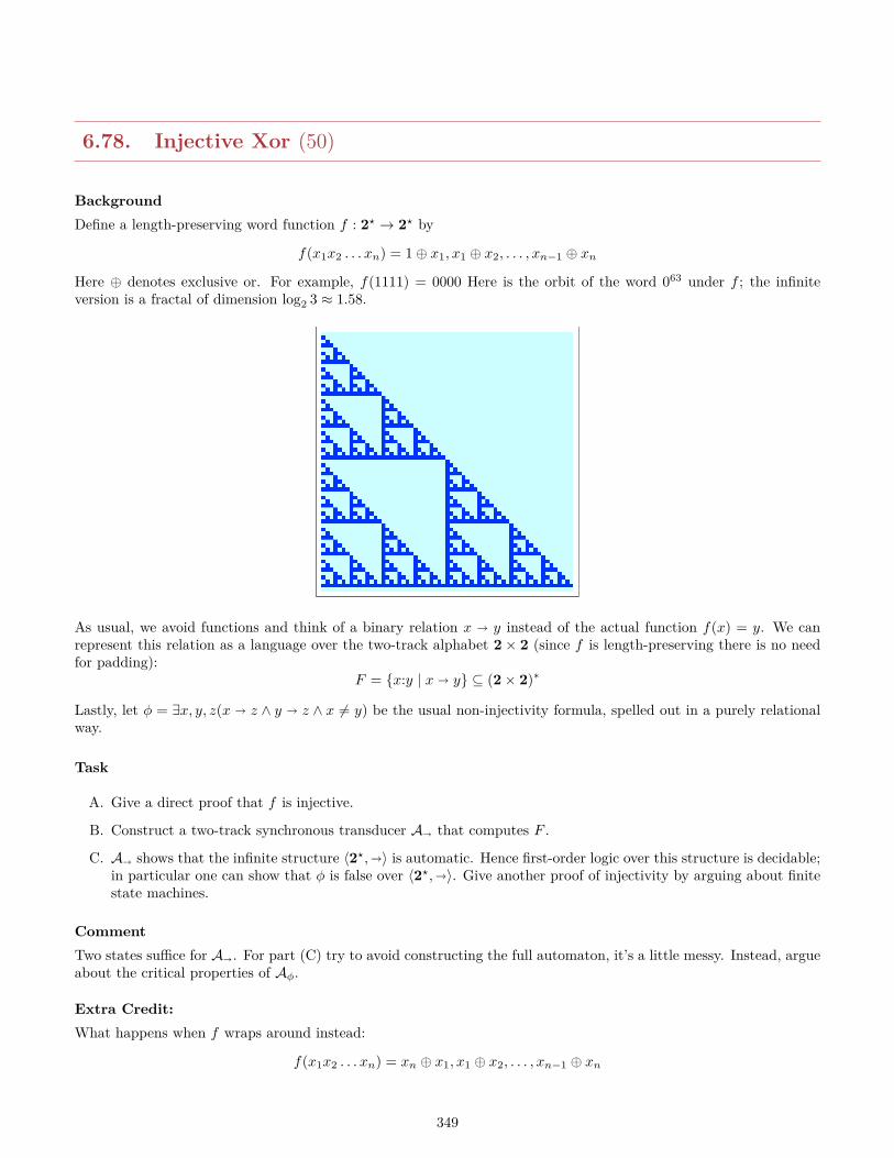
6.78. Injective Xor (50)

BackgroundDefine a length-preserving word function f : 2? → 2? by

f(x1x2 . . . xn) = 1⊕ x1, x1 ⊕ x2, . . . , xn−1 ⊕ xn

Here ⊕ denotes exclusive or. For example, f(1111) = 0000 Here is the orbit of the word 063 under f ; the infiniteversion is a fractal of dimension log2 3 ≈ 1.58.

As usual, we avoid functions and think of a binary relation x y instead of the actual function f(x) = y. We canrepresent this relation as a language over the two-track alphabet 2× 2 (since f is length-preserving there is no needfor padding):

F = x:y | x y ⊆ (2× 2)∗

Lastly, let φ = ∃x, y, z(x z ∧ y z ∧ x 6= y) be the usual non-injectivity formula, spelled out in a purely relationalway.

Task

A. Give a direct proof that f is injective.

B. Construct a two-track synchronous transducer A that computes F .

C. A shows that the infinite structure 〈2?,〉 is automatic. Hence first-order logic over this structure is decidable;in particular one can show that φ is false over 〈2?,〉. Give another proof of injectivity by arguing about finitestate machines.

CommentTwo states suffice for A. For part (C) try to avoid constructing the full automaton, it’s a little messy. Instead, argueabout the critical properties of Aφ.

Extra Credit:What happens when f wraps around instead:

f(x1x2 . . . xn) = xn ⊕ x1, x1 ⊕ x2, . . . , xn−1 ⊕ xn

349

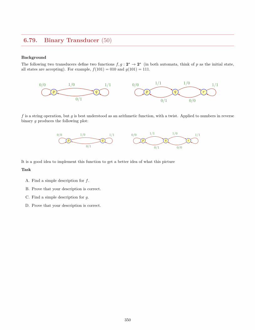
6.79. Binary Transducer (50)

BackgroundThe following two transducers define two functions f, g : 2? → 2? (in both automata, think of p as the initial state,all states are accepting). For example, f(101) = 010 and g(101) = 111.

p q

0/0 1/0

0/1

1/1

p q r

1/1

0/1

1/0

0/0

0/0 1/1

f is a string operation, but g is best understood as an arithmetic function, with a twist. Applied to numbers in reversebinary g produces the following plot:

p q

0/0 1/0

0/1

1/1

p q r

1/1

0/1

1/0

0/0

0/0 1/1

It is a good idea to implement this function to get a better idea of what this picture

Task

A. Find a simple description for f .

B. Prove that your description is correct.

C. Find a simple description for g.

D. Prove that your description is correct.

350

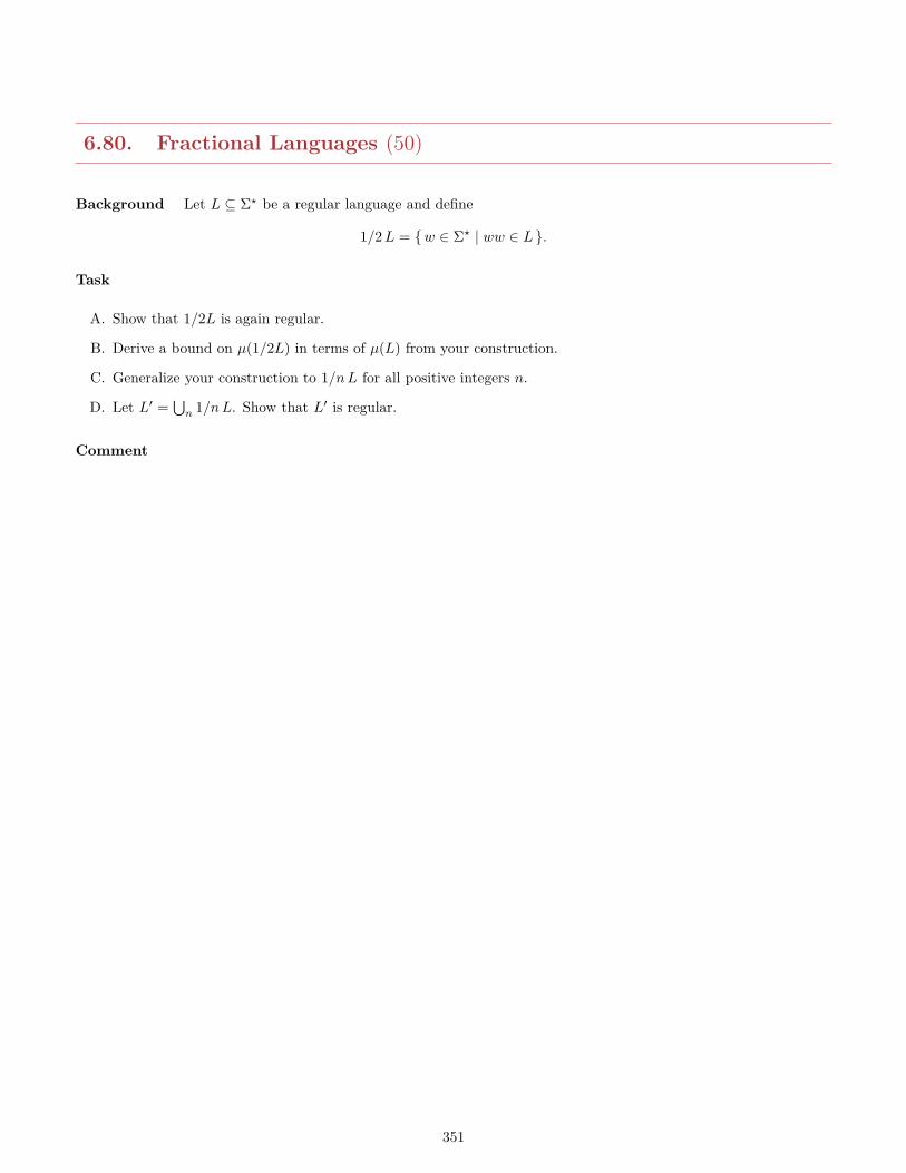
6.80. Fractional Languages (50)

Background Let L ⊆ Σ? be a regular language and define

1/2L = w ∈ Σ? | ww ∈ L .

Task

A. Show that 1/2L is again regular.

B. Derive a bound on µ(1/2L) in terms of µ(L) from your construction.

C. Generalize your construction to 1/nL for all positive integers n.

D. Let L′ =⋃n 1/nL. Show that L′ is regular.

Comment

351

6.81. Counting with DFAs (30)

BackgroundDFAs cannot count in the general sense, but some simple counting tasks can be solved by DFAs. Here is a verygeneral way of describing these easy counting tasks. Let t ≥ 0 and p ≥ 1 be integers, and suppose we have setsA ⊆ 0, . . . , t− 1 and B ⊆ 0, . . . , p− 1Then we can define the semilinear set given by (t, p, A,B) as follows:

S = S(t, p, A,B) = a+ t+ ip+ b | a ∈ A, b ∈ B, i ≥ 0

Thus, A represents “special cases” and B repeats periodically with period p and offset t.Given a semilinear set S, define

L1 = x ∈ a? | #x ∈ S L2 = x ∈ a, b? | #ax ∈ S L3 = x ∈ a, b? | #abax ∈ S

For K, the occurrences of aba are allowed to overlap.

Task

A. Construct a DFA for L from the parameters (t, p, A,B).

B. Construct a DFA for K from the parameters (t, p, A,B).

352

6.82. Divisibility (40)

BackgroundNumbers written in base B ≥ 2 can be construed as words over a digit alphabet D = 0, 1, . . . , B − 1. We canassociate a numerical value to such a string via

val(x1x2 . . . xn) =n∑i=1

2n−ixi

This corresponds to the MSD being first in the string (a really bad idea, but standard notation). Alternatively, wecan place the MSD at the end:

valR(x1x2 . . . xn) =n∑i=1

2i−1xi

This is referred to as reverse base-B notation.Now suppose we have a number given in either base-B or reverse base-B notation. We would like to test whether thenumber is divisible by some modulus m ≥ 1.

Task

A. Construct a DFA that accepts x iff val(x) = 0 (mod m).

B. Construct a DFA that accepts x iff valR(x) = 0 (mod m).

CommentIt is difficult to describe the state complexity of these languages, just build a natural DFA without worrying muchabout its size.

353

Chapter 7

Cellular Automata

354

7.1. Analyzing LFSRs (40)

BackgroundConsider LFSRs with characteristic 2 and span k (as always, assume that there is a tap at the last register). Then theglobal map is injective and the diagram of the global map is just a decomposition of 2k into disjoint cycles. For largespan, experimental verification of the properties of LFSRs is computationally infeasible, but for small k one can easilycompute these cycles. Hence we can determine, for each given LFSR, the average cycle length and the maximum cyclelength.

Task

A. Find all LFSRs of span k = 10 that maximize the maximum cycle length.

B. Find all LFSRs of span k = 10 that maximize the average cycle length.

C. Any observations regarding items (A) and (B)? What is going on?

D. Find all LFSRs of span k = 10 that minimize the average cycle length. Hint: there is exactly one.

E. Explain how this LFSR from part (D) works and how one can compute the average cycle for this type of LFSRdirectly for all k, without simulation.

CommentUnless you are Gauss or von Neumann you will probably want to write a program that computes the cycle decom-position for all the 512 LFSRs in question. For part (E) you do not have to prove that the LFSRs there are in factalways the ones that minimize the average cycle length, just figure out how to compute the average cycle length.

Extra CreditExplain how the LFSR that produces the second lowest average cycle length works.

Needless to say, this problem calls for a bit of experimental computation; doing this by reasoning alone is hard.

355

7.2. Affine Shift Registers (50)

BackgroundLFSRs have two major advantages: they are lightning fast and there is a good theory to analyze them. Alas, sincethe underlying functions are linear, there are problems in particular in applications to cryptography (such as streamciphers). One natural response to such problems is to make the feedback function more complicated (but keep thegeneral feedback-shift mechanism).Prof. Dr. Wurzelbrunft has suggested a solution for these problems: replace linear feedback functions by affinefeedback functions of the form

f(x) = xp1 + xp2 + . . .+ xpr + 1 mod 2

In other words, Wurzelbrunft is suggesting to complement the output bit of the feedback function to define a globalmap F : 2k → 2k . Note that f(0) = 1 so that 0 is no longer a fixed point for F . The question is: how different is thediagram of F from the diagram of F?

Task

A. For taps 1, 3, 4, 10, span 10, compare the ordinary version of the FSR to the Wurzelbrunft complemented one:determine all cycles in the diagram of F .

B. As usual, choose the taps in the FSR according to some irreducible polynomial. What is the relationship betweenthe maximum period for the standard linear global map F compared to the Wurzelbrunft map F? Why?

C. Should Wurzelbrunft get a patent for his idea? Justify your answer.

CommentA little computational experimentation might sharpen your intuition quite a bit in this case – there will be an obviousclaim which turns out to be easy to prove.

356

7.3. Linear Congruential Generators (50)

BackgroundLCGs are a standard way to generate mildly random numbers by iteration:

xn+1 = a xn + b mod m

The crux of this method is to select the right parameters, otherwise we may encounter catastrophic performance.

Task

A. Suppose m = 2k where k = 32 or k = 64.

B. What are bad/good choices of a and b in this case?

C. Now suppose m is a prime, say, a bit smaller than 232. What are bad/good choices of a and b in this case?

D. In general, what are the advantages/disadvantages of using prime moduli as opposed to powers of 2?

CommentA little experimentation may help with this problem, but you might also want to take a look at existing work on thesubject. Don’t write a book.

357

7.4. All-Ones (40)

BackgroundAs we have seen in class, the All-Ones problem has a solution over any grid, and in fact any undirected graph. Forsome simple grids such as narrow strips one can give a direct, geometric solution without having to resort to linearalgebra.

Task

A. Find all solutions of the All-Ones problem for grids of the form 2× n.

B. Find all solutions of the All-Ones problem for grids of the form 3× n.

C. Suppose the solution for the n×m grid is not unique. Show that the solution for the (2n+ 1)×m grid cannotbe unique either. Hint: look at the sum of two solutions.

358

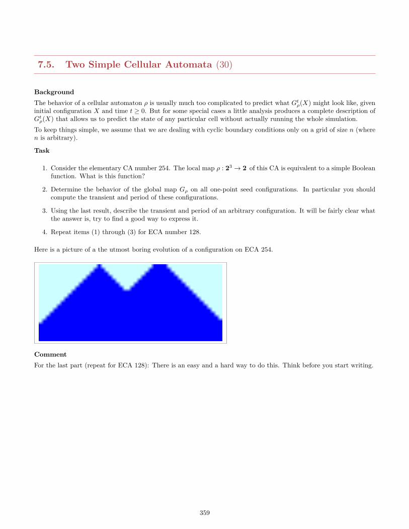
7.5. Two Simple Cellular Automata (30)

BackgroundThe behavior of a cellular automaton ρ is usually much too complicated to predict what Gtρ(X) might look like, giveninitial configuration X and time t ≥ 0. But for some special cases a little analysis produces a complete description ofGtρ(X) that allows us to predict the state of any particular cell without actually running the whole simulation.To keep things simple, we assume that we are dealing with cyclic boundary conditions only on a grid of size n (wheren is arbitrary).

Task

1. Consider the elementary CA number 254. The local map ρ : 23 → 2 of this CA is equivalent to a simple Booleanfunction. What is this function?

2. Determine the behavior of the global map Gρ on all one-point seed configurations. In particular you shouldcompute the transient and period of these configurations.

3. Using the last result, describe the transient and period of an arbitrary configuration. It will be fairly clear whatthe answer is, try to find a good way to express it.

4. Repeat items (1) through (3) for ECA number 128.

Here is a picture of a the utmost boring evolution of a configuration on ECA 254.

CommentFor the last part (repeat for ECA 128): There is an easy and a hard way to do this. Think before you start writing.

359

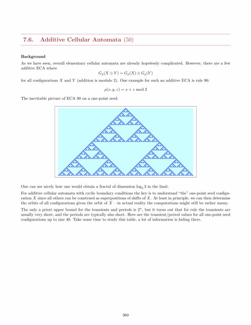
7.6. Additive Cellular Automata (50)

BackgroundAs we have seen, overall elementary cellular automata are already hopelessly complicated. However, there are a fewadditive ECA where

Gρ(X ⊕ Y ) = Gρ(X)⊕Gρ(Y )

for all configurations X and Y (addition is modulo 2). One example for such an additive ECA is rule 90:

ρ(x, y, z) = x+ z mod 2

The inevitable picture of ECA 90 on a one-point seed:

One can see nicely how one would obtain a fractal of dimension log2 3 in the limit.For additive cellular automata with cyclic boundary conditions the key is to understand “the” one-point seed configu-ration X since all others can be construed as superpositions of shifts of X. At least in principle, we can then determinethe orbits of all configurations given the orbit of X – in actual reality the computations might still be rather messy.The only a priori upper bound for the transients and periods is 2n, but it turns out that for rule the transients areusually very short, and the periods are typically also short. Here are the transient/period values for all one-point seedconfigurations up to size 40. Take some time to study this table, a lot of information is hiding there.

360

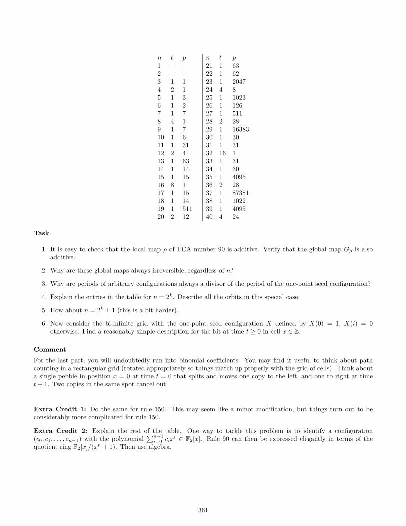
n t p n t p1 − − 21 1 632 − − 22 1 623 1 1 23 1 20474 2 1 24 4 85 1 3 25 1 10236 1 2 26 1 1267 1 7 27 1 5118 4 1 28 2 289 1 7 29 1 1638310 1 6 30 1 3011 1 31 31 1 3112 2 4 32 16 113 1 63 33 1 3114 1 14 34 1 3015 1 15 35 1 409516 8 1 36 2 2817 1 15 37 1 8738118 1 14 38 1 102219 1 511 39 1 409520 2 12 40 4 24

Task

1. It is easy to check that the local map ρ of ECA number 90 is additive. Verify that the global map Gρ is alsoadditive.

2. Why are these global maps always irreversible, regardless of n?

3. Why are periods of arbitrary configurations always a divisor of the period of the one-point seed configuration?

4. Explain the entries in the table for n = 2k. Describe all the orbits in this special case.

5. How about n = 2k ± 1 (this is a bit harder).

6. Now consider the bi-infinite grid with the one-point seed configuration X defined by X(0) = 1, X(i) = 0otherwise. Find a reasonably simple description for the bit at time t ≥ 0 in cell x ∈ Z.

CommentFor the last part, you will undoubtedly run into binomial coefficients. You may find it useful to think about pathcounting in a rectangular grid (rotated appropriately so things match up properly with the grid of cells). Think abouta single pebble in position x = 0 at time t = 0 that splits and moves one copy to the left, and one to right at timet+ 1. Two copies in the same spot cancel out.

Extra Credit 1: Do the same for rule 150. This may seem like a minor modification, but things turn out to beconsiderably more complicated for rule 150.

Extra Credit 2: Explain the rest of the table. One way to tackle this problem is to identify a configuration(c0, c1, . . . , cn−1) with the polynomial

∑n−1i=0 cix

i ∈ F2[x]. Rule 90 can then be expressed elegantly in terms of thequotient ring F2[x]/(xn + 1). Then use algebra.

361

7.7. Affine Cellular Automata (10)

BackgroundSuppose G : C → C is a linear map where C = [n] → 2 is vector space over F2. Given any fixed vector b ∈ C we candefine a new map

F (x) = G(x) + b

Clearly, F reversible if, and only if, G is.

Task

A. Suppose G is reversible and has order m. Show the the order of F is at most 2m.

B. Show that the elementary cellular automata number 60 and number 195 are both reversible on any finite gridwith fixed boundary conditions.

C. Show the hybrid cellular automaton where even-numbered cells use rule 60 and odd-numbered cells use rule 195is reversible on any finite grid, again with fixed boundary conditions.

Comment

362

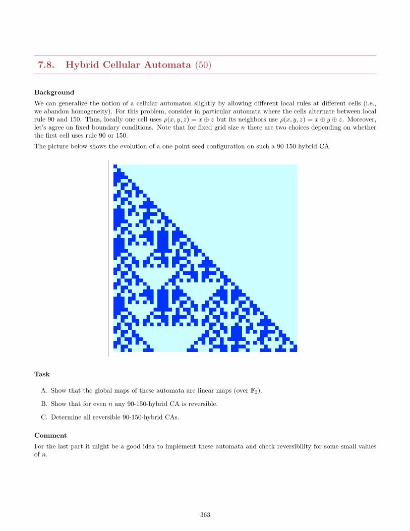
7.8. Hybrid Cellular Automata (50)

BackgroundWe can generalize the notion of a cellular automaton slightly by allowing different local rules at different cells (i.e.,we abandon homogeneity). For this problem, consider in particular automata where the cells alternate between localrule 90 and 150. Thus, locally one cell uses ρ(x, y, z) = x ⊕ z but its neighbors use ρ(x, y, z) = x ⊕ y ⊕ z. Moreover,let’s agree on fixed boundary conditions. Note that for fixed grid size n there are two choices depending on whetherthe first cell uses rule 90 or 150.The picture below shows the evolution of a one-point seed configuration on such a 90-150-hybrid CA.

Task

A. Show that the global maps of these automata are linear maps (over F2).

B. Show that for even n any 90-150-hybrid CA is reversible.

C. Determine all reversible 90-150-hybrid CAs.

CommentFor the last part it might be a good idea to implement these automata and check reversibility for some small valuesof n.

363

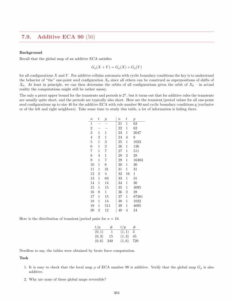
7.9. Additive ECA 90 (50)

BackgroundRecall that the global map of an additive ECA satisfies

Gρ(X + Y ) = Gρ(X) +Gρ(Y )

for all configurations X and Y . For additive cellular automata with cyclic boundary conditions the key is to understandthe behavior of “the” one-point seed configuration X0 since all others can be construed as superpositions of shifts ofX0. At least in principle, we can then determine the orbits of all configurations given the orbit of X0 – in actualreality the computations might still be rather messy.The only a priori upper bound for the transients and periods is 2n, but it turns out that for additive rules the transientsare usually quite short, and the periods are typically also short. Here are the transient/period values for all one-pointseed configurations up to size 40 for the additive ECA with rule number 90 and cyclic boundary conditions g (exclusiveor of the left and right neighbors). Take some time to study this table, a lot of information is hiding there.

n t p n t p1 − − 21 1 632 − − 22 1 623 1 1 23 1 20474 2 1 24 4 85 1 3 25 1 10236 1 2 26 1 1267 1 7 27 1 5118 4 1 28 2 289 1 7 29 1 1638310 1 6 30 1 3011 1 31 31 1 3112 2 4 32 16 113 1 63 33 1 3114 1 14 34 1 3015 1 15 35 1 409516 8 1 36 2 2817 1 15 37 1 8738118 1 14 38 1 102219 1 511 39 1 409520 2 12 40 4 24

Here is the distribution of transient/period pairs for n = 10.

t/p # t/p #(0, 1) 1 (1, 1) 3(0, 3) 15 (1, 3) 45(0, 6) 240 (1, 6) 720

Needless to say, the tables were obtained by brute force computation.

Task

1. It is easy to check that the local map ρ of ECA number 90 is additive. Verify that the global map Gρ is alsoadditive.

2. Why are none of these global maps reversible?

364

3. In the example n = 10, the period of any configurations is a divisor of the period of the one-point seed configu-ration (6 in this case). Is this always the case? Why?

4. Explain the entries in the main table for n = 2k. Describe all the orbits in this special case.

5. How about n = 2k ± 1 (this is a bit harder).

6. Now consider the bi-infinite grid with the one-point seed configuration X defined by X(0) = 1, X(i) = 0otherwise. Find a reasonably simple description for the bit at time t ≥ 0 in cell x ∈ Z.

CommentFor the last part, you will undoubtedly run into binomial coefficients. You may find it useful to think about pathcounting in a rectangular grid (rotated appropriately so things match up properly with the grid of cells). Think abouta single pebble in position x = 0 at time t = 0 that splits and moves one copy to the left, and one to right at timet+ 1. Two copies in the same spot cancel out.

Extra Credit 1: Do the same for rule 150 (exclusive or of all three cells). This may seem like a minor modification,but things turn out to be considerably more complicated for rule 150.

Extra Credit 2: Explain the rest of the table. One way to tackle this problem is to identify a configuration(c0, c1, . . . , cn−1) with the polynomial

∑n−1i=0 cix

i ∈ F2[x]. Rule 90 can then be expressed elegantly in terms of thequotient ring F2[x]/(xn + 1). Then use algebra.

365

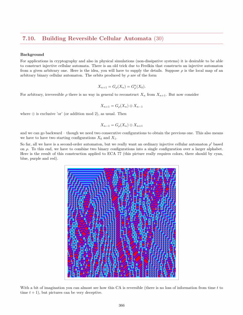
7.10. Building Reversible Cellular Automata (30)

BackgroundFor applications in cryptography and also in physical simulations (non-dissipative systems) it is desirable to be ableto construct injective cellular automata. There is an old trick due to Fredkin that constructs an injective automatonfrom a given arbitrary one. Here is the idea, you will have to supply the details. Suppose ρ is the local map of anarbitrary binary cellular automaton. The orbits produced by ρ are of the form

Xn+1 = Gρ(Xn) = Gnρ (X0).

For arbitrary, irreversible ρ there is no way in general to reconstruct Xn from Xn+1. But now consider

Xn+1 = Gρ(Xn)⊕Xn−1

where ⊕ is exclusive ’or’ (or addition mod 2), as usual. Then

Xn−1 = Gρ(Xn)⊕Xn+1

and we can go backward – though we need two consecutive configurations to obtain the previous one. This also meanswe have to have two starting configurations X0 and X1.So far, all we have is a second-order automaton, but we really want an ordinary injective cellular automaton ρ′ basedon ρ. To this end, we have to combine two binary configurations into a single configuration over a larger alphabet.Here is the result of this construction applied to ECA 77 (this picture really requires colors, there should by cyan,blue, purple and red).

With a bit of imagination you can almost see how this CA is reversible (there is no loss of information from time t totime t+ 1), but pictures can be very deceptive.

366

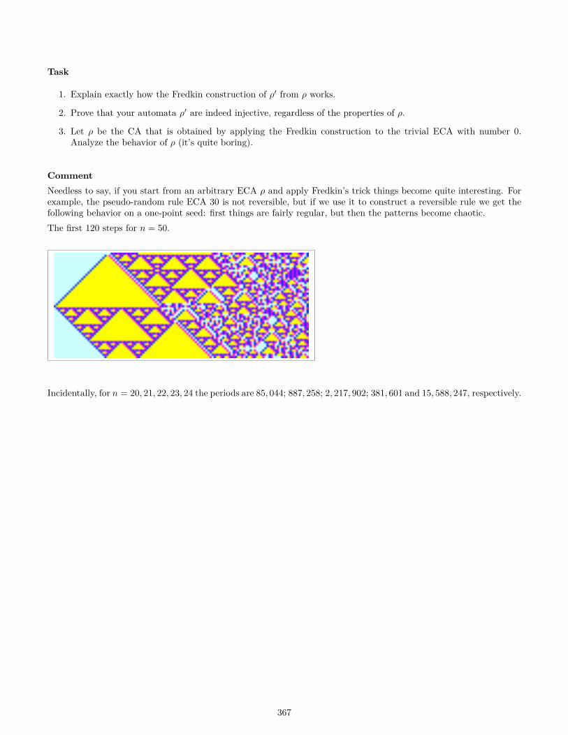
Task

1. Explain exactly how the Fredkin construction of ρ′ from ρ works.

2. Prove that your automata ρ′ are indeed injective, regardless of the properties of ρ.

3. Let ρ be the CA that is obtained by applying the Fredkin construction to the trivial ECA with number 0.Analyze the behavior of ρ (it’s quite boring).

CommentNeedless to say, if you start from an arbitrary ECA ρ and apply Fredkin’s trick things become quite interesting. Forexample, the pseudo-random rule ECA 30 is not reversible, but if we use it to construct a reversible rule we get thefollowing behavior on a one-point seed: first things are fairly regular, but then the patterns become chaotic.The first 120 steps for n = 50.

Incidentally, for n = 20, 21, 22, 23, 24 the periods are 85, 044; 887, 258; 2, 217, 902; 381, 601 and 15, 588, 247, respectively.

367

7.11. Counting Boolean Functions (30)

BackgroundWe have seen how to count Boolean functions modulo the equivalence relation induced by inverting some inputs.Several other modifications produce similar classifications of Boolean functions on k inputs.

Task

1. Count the number of orbits when inputs and the output can be inverted.

2. Count the number of orbits when inputs can be rotated. So if the rotation is by one place we have

f(x1, x2, . . . , xk) = g(x2, x3, . . . , xn, x1)

3. Count the number of orbits when inputs can be arbitrarily permuted.

f(x1, x2, . . . , xk) = g(xπ(1), xπ(2), . . . , xπ(n))

4. Calculate the number of classes

CommentFor the last two problems don’t try to come up with simple closed-form solutions; they don’t exist. But try to writedown the answer concisely and elegantly.

368

7.12. Counting Local Maps (20)

BackgroundOne-dimensional cellular automata are based on local maps Σw → Σ where Σ is some alphabet of size k. Dependingon the kind of analysis one is interested in, one can sometimes cut back on the number of cases one needs to considerby identifying certain kinds of local maps.For example, if ρ(x1, x2, . . . , xw) = ρ′(xw, . . . , x1) then the two local rules are essentially the same (reflection). Likewiseone can ignore rules that are related by a permutation of the alphabet: ρ(x1, x2, . . . , xw) = π−1(ρ′(π(x1), . . . , π(xw))).We are just renaming the symbols here, the dynamics are exactly the same.

Task

1. Count the number of local maps of width w modulo reflection.

2. Count the number of local maps of width w modulo cyclic permutations of the alphabet. To simplify matters alittle, let’s apply the permutation only to the input: ρ(x1, x2, . . . , xw) = ρ′(π(x1), . . . , π(xw)) where π is a cyclicpermutation of Σ.

CommentIf you feel perky, try part two for arbitrary permutations rather than just cyclic ones.

369

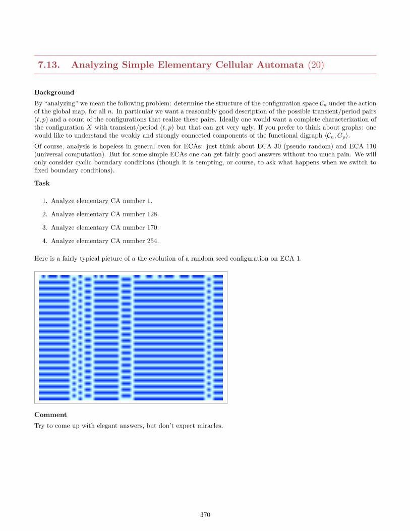
7.13. Analyzing Simple Elementary Cellular Automata (20)

BackgroundBy “analyzing” we mean the following problem: determine the structure of the configuration space Cn under the actionof the global map, for all n. In particular we want a reasonably good description of the possible transient/period pairs(t, p) and a count of the configurations that realize these pairs. Ideally one would want a complete characterization ofthe configuration X with transient/period (t, p) but that can get very ugly. If you prefer to think about graphs: onewould like to understand the weakly and strongly connected components of the functional digraph 〈Cn, Gρ〉.Of course, analysis is hopeless in general even for ECAs: just think about ECA 30 (pseudo-random) and ECA 110(universal computation). But for some simple ECAs one can get fairly good answers without too much pain. We willonly consider cyclic boundary conditions (though it is tempting, or course, to ask what happens when we switch tofixed boundary conditions).

Task

1. Analyze elementary CA number 1.

2. Analyze elementary CA number 128.

3. Analyze elementary CA number 170.

4. Analyze elementary CA number 254.

Here is a fairly typical picture of a the evolution of a random seed configuration on ECA 1.

CommentTry to come up with elegant answers, but don’t expect miracles.

370