1

Chain-Consistent Tight Bounds of True Index Numbers of Productivity:

An Application to EU KLEMS Data

By Carlo Milana°

Abstract

It has been seldom recognized, after an early clarification made by Samuelson

(1947, p. 151) and successive systematic developments of Afriat, that chain-

consistent relative price levels can be reconstructed (up to a constant) using

several observation points directly and simultaneously. The derived ratios of

price levels are mutually consistent by construction and thereby satisfy the

circularity or transitivity test as well as other desirable requirements. By

contrast, to the best of our knowledge, all the other existing index number

methods fall into the realm of the so-called “impossibility theorem”, failing in

particular the circularity test intrinsically. This paper builds on the recent

reappraisal of this approach by Afriat and Milana (2008) and compares it with

akin non-parametric techniques that are based on revealed preferences. An

application to productivity measurement using EU KLEMS data highlights

the usefulness of the method.

Key words: Aggregation, Index number theory Non-parametric analysis,

Price level, Price index, Productivity measurement.

1. Introduction

The aim of this paper is to construct and apply empirically chain consistent tight

upper and lower bounds of “true” measures of productivity in a multilateral setting.

The analysis starts from the recognition that any index number formula may be

potentially unsuitable as an approximation of the unknown “true” index, if this exists

at all. We can, however, identify the tight upper and lower bounds, if any, and test

simultaneously the consistency of the data with aggregation conditions.

The approach presented here is derived directly from that defined by Afriat (2005)

and applied by Afriat and Milana (2008). It is much simpler and appears to be more

convenient than the usual non-parametric deterministic methods based on the ° Istituto di Studi e Analisi Economica, Rome, and Department of Management, Birkbeck

University of London, e-mail address: carlo.milana@iol.it. This paper, has been prepared for the

EU KLEMS project funded by the European Commission, Research Directorate General as part

of the 6th Framework Programme and for presentation at the 2008 World Congress on National

Accounts and Economic Performance Measures for Nations, Key Bridge Marriott, Washington

D.C., May 13-17, 2008. The views expressed in this paper are not necessarily those of the

institutions and persons mentioned here.

2

“revealed preference” theory originally associated with Samuelson

(1938a)(1938b)(1938c)(1947)(1948) and Afriat (1967b)(1972)(1977) himself and

with the further clarifications of Diewert (1973) and Varian (1982)(1983)(1984).

Most of these rely on effective observed budget lines rather than (observed and

virtual) budget lines passing through the base observation points. The consistency

with aggregation conditions has appeared to be violated rarely in the literature even in

the domain of consumer behavior. These unexpected results have puzzled by many

authors, who have questioned the power of the test itself.

It is believed that these results have been obtained because income effects, which

tend to dominate the level of demand, overcome the price-induced substitution effects

(see, for example, Varian, 1983, 2006, Blundell et al. 2003, and Blundell, 2005). The

budget lines taken into exam seldom cross each other and, for this reason, there would

be little room for the violation of the “revealed preference” conditions, which is

expected in the general non-homothetic case.

The problem may be avoided by considering that, in the traditional economic

model, the relevant isoquants or indifference curves, if any, are bounded not by the

effective budget lines, but by piecewise linear frontiers passing through the same base

point and representing, at different observed prices, the constant-quantity monetary

income. The algorithm proposed by Afriat offers a way to construct tight upper and

lower bounds of the unknown “true” economic index numbers, if the aggregation

conditions are satisfied. The two piecewise linear bounds may themselves be good

candidates of representing the “true” index number. From the point of view of this

approach, the question itself of the power of non-parametric tests raised by some

authors arises only because of the nature of the measures used.

In case of inconsistency with aggregation conditions, it is suggested that the

accounting system should be widened in order to be consistent with a more general

set of the variables (by considering, for example, a more complete set of non-

separable outputs and inputs) and, if this is not possible, a correction for allocative

inefficiency is introduced. The proposed method is truly constructive in that it does

not even necessarily require a certain model or the existence of non-observational

objects like utility- or technology-based functions (or the corresponding “dual” value

functions such as optimal cost, revenue, or profit functions).

The alternative index numbers obtained as tight bounds of the unknown “true”

economic index are derived from aggregates of price levels. Since these are by nature

transitive in their ratios or differences, the index numbers that are derived in this way

in a multilateral setting are chain-consistent and therefore satisfy automatically the

requirement of transitivity (or circularity) property. To our knowledge, this approach

is, until now, the only one available in the field of index numbers that satisfies this

requirement directly without further manipulations. The proposed methodology is

applied to the EUKLEMS database, which has been built for the European

Commission covering more than 30 countries at the industry level since 1970.

3

The paper is organized as follows. Section 2 briefly recalls the problems

encountered with multilateral index numbers. Section 3 reviews the Samuelson-

Afriat‟s non-parametric (deterministic) analysis based on revealed preference and the

alternative index number approach presented here. Section 4 describes Afriat‟s power

algorithm and the program performing the empirical computations. Section 5

formulates the problem of multifactor productivity measurement. Section 6 describes

some of the results obtained in productivity measurement using EU KLEMS data.

Section 7 concludes.

2. Aggregation problems with index numbers

Prices (or deflators) and quantities (or volumes) referring to economic aggregates are

not observable. The empirical literature has followed alternative directions to

construct such aggregates, among which the most common are: (i) multiple

observations are introduced simultaneously and analyzed using the Samuelson-Afriat

revealed preference techniques; (ii) assuming specific functional forms about the

underlying economic functions (cost or utility or production functions), the

corresponding “exact” index numbers are applied (using the terminology of

Byushgens, 1924 and Konüs and Byushgens, 1926); (iii) the aggregator functions are

estimated by means of econometric techniques and their numerical values are

assessed by choosing particular levels of reference variables. All these approaches

present serious drawbacks.

Revealed preference techniques are primarily used to test the compatibility of the

data with the rational behaviour hypothesis as well as for linear homogeneity and

separability restrictions, which are necessary and sufficient for the existence of an

economic aggregator function. In the empirical literature, these analytical techniques

routinely fail to reject homotheticity, thus suggesting that there is something wrong

with the assumptions on the behaviour generating the data and/or with the method

itself, which appears not to be demanding enough for various reasons. The power of

the so-called Afriat-Varian test is considered too low so that some authors have tried

to extend it in order to take account of non-homothetic changes.

The economic index number approach assumes an underlying specific well-

behaved functional form of the aggregator function and identifies the corresponding

exact index number. This approach gives rise to a joint test of the specific functional

form and the fundamental requirements for the measures obtained. Given the

assumptions made, the failure to satisfy the requirements cannot be attributable to the

data or the model taken separately from the particular specification of the functional

form. Moreover, the interpretation of the index numbers formulas as being exact for

aggregator functions providing approximations of the “true” measure presents its own

limits, as pointed out by a number of analysts. This applies also to the class of the

“superlative” index numbers that are supposed to provide approximations up to the

4

second order (see, for example, Afriat, 1977, Uebe, 1978, Neary, 2004, Milana, 2005,

Hill, 2006a, Afriat and Milana, 2008).

The economic approach assumes that the prices represented here with the vector p

and the respective quantities q of demanded goods are consistent with maximization

of utility, which is a well-behaved (concave) function of the quantities q, let us say

( )q , governing the demand subject to the budget constraint given by total income

i ii

E pq p q . This could also be seen as minimization of expenditure subject to a

given utility, that is

( , ) : ( )qE p u Min pq q u , (1)

where u is the given utility.

Following Samuelson and Swamy (1974, p. 570), for a given value function ( , )E p u ,

meaningful aggregates of p and q can be constructed using the following results:

Rule (i): ( , )pq E p u by Shephard’s lemma (established under the hypothesis of

optimizing behaviour), which describes the demand of q as functions of prices and

utility, governed by preferences represented by the function ( )f q under the constraint

of disposable income whose value is equal to pq .

Rule (ii): ( , ) ( ) ( )E p u e p f q by Shephard-Afriat’s factorization theorem

(established under the hypothesis of homotheticity of the utility function ( )f q ). This

rule defines the invariancy of the aggregator functions e(p) and f(q) with respect to the

reference variables u and p respectively1. As Samuelson and Swamy (1974, p. 570)

have recognized, “[t]he invariance of the price index is seen to imply and to be

implied by the invariance of the quantity index from its reference price base”.

Under the rules (i) and (ii), economic index numbers 0tP and 0tQ can be

constructed, which are called “exact” for the aggregator functions ( )e p and ( )f q ,

respectively, as they are identically equal to the ratios of the values taken by the

aggregates at two observed points, that is 0

0

( )

( )

tt

e pP

e p and 0

0

( )

( )

tt

f qQ

f q . As noted by

Samuelson and Swamy (1974, p. 573, fn. 9) and Diewert (1976, pp. 132-133), all

Fisher‟s tests are satisfied by all economic index number formulas (when these are

1 Homotheticity and identical preferences seem, however, to have been noticed as early as the

work of Antonelli (1886) as necessary and sufficient conditions for aggregation if this is to hold

globally. Conditions for aggregation holding only locally and allowing preference eterogeneity

have been studied by Afriat (1953-56) (1959) and Gorman (1953, 1961).

5

“exact” for the true aggregator functions in the homothetic case). Also the circularity

test is satisfied, that is 20 21 10P P P

as

2 1 2

0 0 1

( ) ( ) ( )

( ) ( ) ( )

e p e p e p

e p e p e p with

( )

( )

iij

j

e pP

e p (2)

In principle, Byushgens (1924) and Konüs and Byushgens (1926) have introduced

the concept of “exact” index numbers for the true aggregator function by showing that

the popular index number formulas such as the Fisher “ideal” index number may

yield the same numerical values of a specific aggregator function. Following Diewert

(1976), let us assume that the aggregator function e(p) has, for example, a quadratic

mean-of-order-r functional form, that is / 2 / 2 1/( ) ( )r

r r r

Qe p p Ap , where

0, 0 < r r , with A being a symmetric matrix whose positive elements

ija satisfy the restriction ' 1A , where [11...1], so that ( ) 1rQe p if p .

We recall that McCarthy (1967) and Kadiyala (1972) considered the functional

form ( )rQe p as a generalization of a CES functional form, to which it is equivalent if

all 0ija for i j2.

We have in fact

1

0

( )

( )

r

r

Q

Q

e p

e p=

1// 2 / 2

1 1

1// 2 / 2

0 0

rr r

rr r

p Ap

p Ap

1// 2 / 2 / 2 / 2

1 1 1 0

/ 2 / 2 / 2 / 20 1 0 0

rr r r r

r r r r

p Ap p Ap

p Ap p Ap

since / 2 / 2 / 2 / 21 0 0 1r r r rp Ap p Ap with a symmetric A

1// 2 / 2 / 2 1 / 2 / 2 1 / 2

1 1 1 0 0 0

/ 2 1 / 2 / 2 1 / 2 / 2 / 20 1 1 1 0 0

ˆ ˆ

ˆ ˆ

rr r r r r r

r r r r r r

p Ap p p p Ap

p p p Ap p Ap

where ^ denotes a diagonal matrix

formed with the elements of a vector 1

/ 21

0/ 20

0 1 0 1 / 20

1/ 21

( , , , )r

r ri

irii

Q r

iri

ps

pP p p q q

ps

p

(3)

2 Moreover, Denny (1972)(1974) noted that, if ,1r then

/ 2 / 2 1/( ) ( )r

r r r

Qe p p Ap reduces to the

Generalized Leontief functional form proposed by Diewert (1969)(1971). Diewert (1976, p. 130)

himself noted that, if ,2r then it reduces to the Konüs-Byushgens (1926) functional form.

6

where

/ 2 / 2

/ 2 / 2

r rti ij tj

jti titi r r

t ttj tjj

p a pp qs

p App q

(with ija being the (i,j) element of matrix A),

which is the observed value share of the ith quantity

1/ 22

11

/ 2 / 2

( )( , ) / ( ) ( )

( )

r

r

rij tjtiQ j

ti ti

ti r r rt t

p a pe pq E p u p f q f q

pp Ap

by Shephard‟s lemma. The

resulting formula 0 1 0 1( , , , )rQP p p q q is Diewert‟s (1976, p.131) quadratic mean-of-

order-r index number,

The quadratic mean-of-order-r index number 0 1 0 1( , , , )rQP p p q q encompasses the

class of all the index numbers that Diewert (1976) has called “superlative”, which are

exact for polynomial aggregator functions of degree up to the second order3.

However, as already noted by Afriat (1956)(1967a) in the case of Fisher “ideal” index

and Uebe (1978), starting from the index 0 1 0 1( , , , )rQP p p q q , we cannot fully recover a

polynomial of second order (with non-zero second derivatives) to represent the

underlying aggregator function ( )rQe p . The index 0 1 0 1( , , , )rQ

P p p q q is constructed

using the information of 2N-2 independent data concerning the weights 0 1 and s s ,

with N representing the number of items to be aggregated. By contrast, the

underlying function ( )rQe p has N(N+1)/2-1 independent elements in the symmetric

matrix A, plus the power exponent r. With this last parameter exogenously given

(assumed a priori), the free parameters outnumber the independent data concerning

the weights when 2.N Therefore, the numerical value of the index

0 1 0 1( , , , )rQP p p q q is arbitrarily determined by the choice of the value of r even with the

minimum number of elements is set equal to 2. Moreover, solving the differential

equations derived from the function ( )rQe p for the elements of matrix A yields:

1 / 2 1

1

( )2

ij i j

ij

r ri j

re e e

ear

e p p

for , 1,2, ...,i j N (4)

where ( )rQe e p ,

( )rQ

k

k

e pe

p

and

2 ( )rQ

ij

i j

e pe

p p

. Since non-zero elements ija are

possible even if 0,ijC all the elements of the matrix A can be determined without

3 Diewert (1976, p. 135) noted that, if 1,r 0 1 0 1( , , , )rQ

P p p q q reduces to the implicit Walsh

(1901, p. 105) index number (this index is exact for the Generalized Leontief aggregator

function), and, if 2,r then it reduces to the Fisher (1922) “ideal” index number (the geometric

mean of the Laspeyres and Paasche indexes), which is exact for the Konüs-Byushgens (1926)

aggregator function.

7

the need to have non-zero second-order derivatives. This implies that the same index

0 1 0 1( , , , )rQP p p q q for a given price and quantity data set could be equally “exact” for

first-order and second-order polynomial aggregator functions. In other words, the

superlativeness of the index 0 1 0 1( , , , )rQP p p q q is not guaranteed even in the homothetic

case.

In an unpublished memorandum, Lau (1973) showed that, at the limit as r tends

to zero, the functional form ( )rQe p reduces to the homogeneous translog aggregator

function so that

0 0

1lim ( ) ( ) exp[ ln ln ' ln ]

2rr TQ

e p e p a p p A p (5)

Lau‟s proof is reported in Diewert (1980, p. 451) (see Milana, 2005 for an alternative

proof).

Then

1

1 ' '0 1 0 0 1 1

0

( ) 1lim exp[ln ( ) ln ( )] exp[ ln ln ln

( ) 2

r

r

Q

r T T

Q

e pe p e p a p p A p

e p

0 0 0 0

1ln ln ' ln ]

2a p p A p

0 1 0 1 0 1 0

1exp[( ln )(ln ln ) (ln ln ) (ln ln )]

2a p A p p p p A p p

1 1 0 1 0 1 0

1exp[( ln )(ln ln ) (ln ln ) (ln ln )]

2a p A p p p p A p p

0 1 1 0

1exp[ [( ln ) ( ln )](ln ln )] taking the geometric average of the previous two lines

2a p A a p A p p

ln 0 ln 0 1 0

1exp[ [ ( ) ( )](ln ln )]

2p T p Te p e p p p

0 1 0 1 0 1 1 0

1( , , , ,) exp[ [ ](ln ln )]

2TP p p q q s s p p , which is the the Törnqvist index,

since ( )

ln ( ) / ln( )

T iT i

i T

e p pe p p

p e p

( )( )

( ) ( )

T i

i T

e p pf q

p e p f q

ii i

i ii

ps q

p q

by Shephard‟s lemma, with ( ) ( )Te p f q i iip q by Shephard-Afriat‟s factorization

theorem.

An identification problem can be met with the true aggregator as a second-order

polinomial function can be met starting also from the index number 0 1 0 1( , , , ,)TP p p q q .

Following Uebe (1978), we can note that the superlativeness character of this index

number cannot be present even in the homothetic case.

8

In empirical applications the above superlative index numbers generally fail to

pass the circularity test. Fisher (1922) himself had noted that its “ideal” index

number does not generally satisfy this test. Yet, as we have recalled above, if it is

consistent with the data that are generated by an optimized behaviour governed by a

homothetic utility and an expenditure function having a quadratic mean-of-order-2

functional form, at least locally, so that 2 0 1 0 1 10( , , , )Q

P p p q q P , then also this index

number should exhibit the transitivity property. Samuelson and Swamy (1974, p. 575)

wittingly observe: “Where most of the older writers balk, however, is at the circular

test that frees us from one base year. Indeed, so enamoured did Fisher become with

his so-called Ideal index 1/ 21 0 0 0 1 1 0 1[( / / )( / / )]p q p q p q p q = square root of

(LaspeyresPaasche) that, when he discovered it failed the circular test, he had the

hubris to declare „…, therefore, a perfect fulfillment of this so-called circular test

should really be taken as proof that the formula which fulfills it is erroneous‟ (1922,

p. 271). Alas, Homer has nodded; or, more accurately, a great scholar has been

detoured on a trip whose purpose was obscure from the beginning”.

The circularity test may be violated either because the economic agent is not

optimizing and/or the utility or technology function is non-homothetic, non-separable

in the variables of interest and/or the chosen index number formula is not “exact” for

the “true” aggregator function. This fact has been very seldom recognized in the

economic literature even long after the notion of the exact index numbers has been

discovered by Byushgens (1924) and Konüs and Byushgens (1926). This has

prevented a widespread use of the circularity test as an empirical refutation of the

aggregation conditions. We must emphasize the importance of this test as a first step

to address the problem of aggregation correctly.

Violation of the circularity test may lead to severe problems of inconsistency not

only in absolute levels of quantity indexes, but also in their relative ranking position.

In a multilateral context, various methods have been devised so far to eliminate the

inconsistencies of the results obtained. Most of them remain bilateral in nature,

disguised in a multilateral dressing. Among these, we may mention the so-called star

system where each observed point is compared with one observed or a hypothetical

average point as in the so-called EKS and CDD methods, based respectively on the

use of bilateral Fisher “ideal” and Törnqvist indexes. In these last two methods, the

hypothetical average point used for an intermediate comparison is implicitly

constructed as an average of all points. The main problem with these methods is the

same as that encountered with bilateral index numbers that are not well grounded on

the aggregation conditions. In the non-homothetic case, the conditions for the

Shephard-Afriat‟s factorization theorem do not hold. Therefore, the aggregator

functions of prices and quantities are not well defined and, if we insist in constructing

bilateral (economic) index numbers based on value functions (expenditure, profit or

revenue functions), we will obtain spurious magnitudes of price and quantity

aggregates being functions not only of individual prices and quantities respectively,

9

but also of reference variables. This can be seen, for example, by inspecting the

equations of the value shares s used as weights in the index number formulas

considered above. In the non-homothetic case, the expenditure function cannot be

decomposed into distinct terms of prices and utility. The quantities are obtained as

follows

( , ) /ti tiq E p u p by Shephard‟s lemma (6)

with the shares given by

( , )

( , )

t t tiit

ti t t

E p u ps

p E p u

(7)

which are functions not only of prices but also of the reference utility. They should be

contrasted with the homothetic case where they are functions only of prices so that the

aggregator function exists as a pure price component. A clear separation of price and

quantity components of the total value changes is possible only in the special case of

homothetic separability4. These conclusions differ from those of Caves, Christensen

and Diewert (1982a)(1982b) and Diewert and Morrison (1986), where this distinction

is not made5.

When homothetic separability conditions are not met, any attempt to obtain

deflated values by constructing linearly homogeneous quantity index numbers (using

for example distance functions) would inevitably lead us to failure in satisfying the

exhaustiveness requirement, which is better known in the literature as (weak) factor

reversal test: the total value should be identically equal to the total contribution of the

aggregate components. Our problem is to decompose the relative or absolute change

in the scalar value t t ti tip q p q between t=0 and t=1 into a scalar price-change

component and a scalar quantity-change component starting from the change in the

single elements of the two vectors tp and tq , that is

1 1 0 0 0 1 0 1 0 1 0 1( , , , ) ( , , , )i i i i P Qp q p q p p q q q q p p (8)

4 This is related to the well-known conclusion reached by Hulten (1973) on path-independency

of Divisia indexes in the case of homothetic functions (see Milana, 1993 for further explanatory treatment). 5 In the non-homothetic case, we might attempt to construct an aggregating linearly homogeneous

quantity index numbers (price index numbers are always linearly homogeneous by construction). This is a procedure followed, for example, by Caves et. al. (1982) in defining their input quantity and price index numbers. However, the indexes thus obtained are not pure quantity and price components.

10

where 0 1 0 1( , , , )P p p q q and 0 1 0 1( , , , )Q q q p p are the additive price and quantity

components of the absolute change in the scalar value pq, and

1 1

0 1 0 1 0 1 0 1

0 0

( , , , ) ( , , , )i i

i i

p qP p p q q Q q q p p

p q

(9)

where 0 1 0 1( , , , )P p p q q and 0 1 0 1( , , , )Q q q p p are the moltiplicative price and quantity

components of the relative change in the scalar value pq. These price and quantity

components should be appropriate pure aggregates of the changes in the elementary

prices and elementary quantities, respectively: each of these two aggregating

components should not contain elements of the other. If changes in relative quantities

are affected only by changes in relative prices, as it happens in the homothetic case,

then the change in the scalar value t

i

t

i qp can be split, at least in theory, in two

price and quantity components, representing proportional (scale) price and quantity

factors, respectively. By contrast, if changes in quantities are affected not only by

relative prices, but also by some “external” or “reference” variable in a non-

homothetic way, then it is impossible to disentangle completely the effects on

quantities arising from the changes in relative prices and the changes in the reference

variable. Any definition and measure of the price and quantity change components

would result to be spurious magnitudes, for each component contains some elements

of the other. Under this condition, the circularity test cannot be generally satisfied.

Pollak (1971), Samuelson and Swamy (1974, 576-77), Archibald (1977), Fisher

(1988)(1995) and Fisher and Shell (1998) had observed that, in the general non-

homothetic case, a side effect of the non-invariancy of the price aggregating index is

that the corresponding quantity index fails to satisfy the requirements of the linear

homogeneity test. For example, if all the single quantities double, the derived quantity

measure fails to double6. This undesired property is a consequence of the fact that, in

the non-homothetic case, the price aggregating index is a spurious index number

which captures not only the changes in prices but also changes in the reference utility

level.

In a later work, Diewert (1983a, pp. 178-179) has recognized that, in the non-

homothetic case, a quantity index number obtained implicitly by deflating the index

of total nominal expenditure by means of an economic price index may not result to

be linearly homogeneous in the elementary quantities. This may occur even if the

deflator is the Törnqvist index.

6 This conclusion is immediate if one considers that the economic index numbers that are derived

from a non-homothetic function could never satisfy, by construction, all the homogeneity

requirements.

11

In searching a way out from this impasse, Diewert (1983a) constructed a cost-

based direct price index and a direct Törnqvist quantity index. This procedure has

been supported by Russell‟s (1983) comments7. Diewert (1983b) followed a similar

procedure in the theory of output price and quantity changes. However, although both

these price and quantity index numbers turn out to satisfy the linear homogeneity

requirement, this outcome is achieved at the cost of failing to satisfy the requirements

of the factor-reversal test (stating that the price index multiplied by the quantity index

should equal the index of total nominal value). Samuelson and Swamy (1974, p. 576)

clearly observed: “If, like Pollak, one employs a quantity definition that satisfies

Fisher‟s (i*) [linear homogeneity test], then [given the imposed linear homogeneity of

the price index] one of the other tests, such as (v*) [weak factor reversal test], will fail

in the nonhomothetic case”. They spelled out this result even more clearly in another

example (p. 577, fn. 10): “Afriat favors the linear Engel-curve approximation:

,)"()()();( PQPQPe where the last additive term is a residual not captured by

the linearly homogeneous price index multiplied by the linearly homogeneous

quantity index.

In consideration of non-homothetic changes in parameters of the underlying

function, Diewert‟s (1976, pp. 123-124) has also shown that the Törnqvist quantity

index can be "exact" for a Malmquist quantity index which is defined by a translog

distance function evaluated at the geometric mean of the utilities in the two compared

points of observation.. This result has been later generalized by Caves, Christensen,

and Diewert (1982, pp. 1409-1413) in their Translog Identity. They showed that the

Törnqvist index number is "exact" for the geometric mean of two translog functions

referred to the two compared points of observation and differing in parameters of

their zero- and first-order terms.

The Törnqvist index is, therefore, still regarded as being equally valid for

measuring aggregate relative changes in input quantities or prices under alternative

assumptions of homothetic and non-homothetic changes. Caves et al. (1982, p. 1411)

claimed: "This result implies that the Törnqvist index is superlative in a considerably

more general sense than shown by Diewert. We are not aware of other indexes that

can be shown to be superlative in this more general sense". However, since all

superlative indexes are supposed to approximate one another numerically, they

conclude: "any superlative index (in the sense of Diewert, 1976) will be

approximately equal to the geometric mean of two Malmquist indexes based on the

translog form". More recently, it has been shown that, in the non-homothetic case, the

Törnqvist index number can be “exact” for a more general weighted geometric mean

of two translog functions differing in all parameters. Contrary to what has been

previously contended, a similar result is also valid for all the other indexes that are

7 Russell (1983, p. 237) concludes that the Malmquist quantity index, which Diewert favours

because of its intrinsic properties, is in fact the only natural counterpart to the widely accepted

Konüs cost-of-living index.

12

encompassed by the quadratic mean-of-order-r index number formula (see Milana,

2005).

Diewert (1976, pp. 123-124) and Caves et. al. (1982) have explicitely recognized

that, in the non-homothetic case, the Translog Identity is not “an if and only if” result,

in sense that an aggregator translog function implies that the corresponding “exact”

index number formula is Törnqvist, but this could be “exact” for functional forms of

the aggregator function other than the translog. The same applies to the other

superlative index number formulas which, as shown in Milana (2005), might as well

be “exact” also to first-order polynomial functional forms subject to non-homothetic

changes. This further weakens the superlativeness character of these index numbers

in such cases.

The problems outlined here may worsen in the context of a multilateral

comparison when (as it generally happens) the circularity test is not passed with the

single bilateral comparisons. Aggregation over inconsistent bilateral comparisons

may lead to a systematic bias. This is, in particular, the case of the EKS and CCD

methods cited above (see, for example, Neary, 2004, pp. 1414-1416).

Another reason why the chosen index number formula does not satisfy the

circularity test is often attributed to the fact it can be exact for some form of

approximation to the “true” index. Diewert (1976, pp. 115-117) has also stressed the

importance of using the index numbers that are “exact” for quadratic functional

forms, which he called flexible, since these may be alternatively interpreted as

second-order approximations to an arbitrary (twice-differentiable) “true” aggregator

function. As shown in Milana (2005), the data on the compared points of observation

are not generally consistent with the approximating aggregator function but account

for the actual economic behavior. This also prevents the so-called “superlative” index

number formula to be exact for a second-order approximating aggregator function.

What is really obtained with this formula is an hybrid index number that can be

interpreted as a combination of two first-order approximations at the two compared

observed points. As Samuelson and Swamy (1974, p. 582) remind us:

“[a]pproximations often violate transitivity. For example, 1.01 and .99 are each within

1 percent approximations to 1.0, but that does not make them have this property with

respect to each other!”.

Allen and Diewert (1981, p. 430) had recognized that “in many applications

involving the use of cross section data or decennial census data, there can be a

tremendous amount of variation in prices or in quantities between the two periods so

that alternative superlative index numbers can generate quite different results”. In

fact, more recently, Hill (2006) has found a large spread in numerical values of

alternative superlative index numbers, with the largest and the smallest ones differing

by more than 100 per cent using a standard US national data set and by about 300 per

cent in a cross-section comparison of countries using an OECD data set. However, it

has been surprising to find empirically that the spread between the largest and the

13

smallest Diewert‟s superlative index numbers may exceed that between the Laspeyres

and Paasche indexes. This performance is clearly in contrast with that considered

originally by Irving Fisher in identifying his own superlative index numbers.

The Fisher “ideal” index itself (the particular case of the quadratic mean-of-order-

r index number where 2r , corresponding to the geometric mean of the Laspeyres

and Paasche indexes) can be a poor approximation to the “true” index in the non-

homothetic case. On this point Samuelson and Swamy (1974, p. 585) clearly wrote:

“It is evident that the Ideal index cannot give high-powered approximation to the true

index in the general, nonhomothetic case. A simple example will illustrate the degree

of this failure […]. [E]ven if (P1,P0,Pα) and (Q1,Q0) are „sufficiently close together, it

is not true that the Laspeyres [λq] and Paasche [πq] indexes provide two-sided bounds

for the true index. In this example, the true index lies outside the [λq, πq] interval!”.

We can attempt to decomposed the relative change in the expenditure function

as follows

1 1

0 0

( , )

( , )p q

E p uI I

E p u (10)

where pI and qI have the meaning of the price and quantity indexes respectively.

Following Milana (2005), any price index number that is exact for a continuous

aggregator function can be translated into the following form

1( ) 1 ( )0

1 0 1 10

1 10 0 0 0 1

1

1

(1 )

(1 )

ii

N Ni i i iip

i ii i i i i

i

i

ps

p q p qpI

p p q p qs

p

(11)

where, for t = 0,1, ( , ) ( , )

/t t t t

ti ti tjjti tj

E p u E p us p p

p p

/ti ti tj tjjp q p q using Shephard‟s lemma

and is an appropriate parameter whose numerical value depends on the

remainder terms of the two first-order approximations of E(p,u) around the base

and current points of observations.

The index pI is linearly homogeneous in p (that is, if 1 0 ,p p then ).pI

With ,0 it reduces to a Laspeyres index number, whereas, with ,1 it reduces

to a Paasche index number.

14

The “true” exact index number, if any, is numerically equivalent to pI . If the

functional form of ( , )t tE p u is square root quadratic in ,p then pI can be

transformed into a Fisher “ideal” index number, which is given by the geometric

mean of the Laspeyres and Paasche index numbers. In this case, the index pI is

numerically equivalent to a quadratic mean-of-order-2 index number.

Here, again, the index pI is invariant with respect to the reference utility level

if and only if ( , )E p u is homothetically separable and can be written

( , ) ( )E p u e p u , in which case /ti ti ti tj tjjs p q p q

( ) (/ .

t tti tjj

ti tj

e p e pp p

p p

Moreover, 1 1 0 0[ ( , ) / ( , )]/q pI E p u E p u I is the quantity index measured implicitly

by deflating the index of the functional value with the price index pI . It has the

meaning of a pure quantity index if and only if pI is a pure price index.

The parameter , however, remains unknown and we cannot rely on the second-

order differential approximation paradigm. For this reason, in a previous paper, we

concluded that “it would be more appropriate to construct a range of alternative index

numbers (including those that are not superlative), which are all equally valid

candidates to represent the true index number, rather than follow the traditional search

for only one optimal formula” (Milana, 2005, p. 44). This conclusion was anticipated

long before by Afriat (1977, pp. 107-112):

“The price index 10P is determined by the utility R and the prices 0 1 and .p p The

condition on R which permits this determination, for arbitrary 0 1 and ,p p is equivalent

to the requirement that the utility-cost function admits the factorization into a product

[ , ] ( ) ( )E p u e p f q (12)

of the price and quantity functions. […] Then the price index, with 0 and 1 as base

and current priods, is expressed as ratio

10 1 0/P P P (13)

of price levels

The conclusion […] is that the price index is bounded by the Paasche and Laspeyres

indices. […] The Paasche index does not exceed the Laspeyers index. […] The set of

values [of the “true index”] is in any case identical with the Paasche-Laspeyres

interval. The “true” points are just the points in that interval and no others; and none

is more true than another. There is no sense to a point in the interval being a better

15

approximation to “the true index” than others. There is no proper distinction of

„constant utility‟ indices, since all these points have that distinction”.

The same conclusion is replicated in Afriat (2005, p. xxiii):

“Let us call the LP interval the closed interval with L [Laspeyers index] and P

(Paasche index] as upper and lower limits, so the LP-inequality is the condition for

this to be non-empty. While every true index is recognized to belong to this interval,

it can still be asked what points in this interval are true? The answer is all of them, all

equally true, no one more true than another. When I submitted this theorem to

someone notorious in this subject area it was received with complete disbelief.

“Here is a formula to add to Fisher‟s collection, a bit different from the others.

“Index Formula: Any point in the LP-interval, if any.”

3. Revealed-preference based tests, recoverability of utility or technology and

index number bounds

The difficulty of finding a satisfactory point estimate of the “true” economic price

index number based on the adoption of specific formulas has led many authors to find

alternative solutions eschewing parametric forms. These alternative solutions are

based on the revealed preference theory originally offered by Samuelson (1938a)

(1938b)(1938c)(1947)(1948) and Houthakker (1950), first implemented empirically

by Houthakker (1963) and Koo (1963).

It was not until the appearance of the fundamental Afriat’s (1967b) theorem that

the revealed preference approach could not be fully exploited empirically starting

from the available data. Rather than assuming the existence of a well-behaved

continuous differentiable (single-valued) utility function governing the demand

generating the observed data, Afriat‟s approach is truly constructive and asks whether

it is possible to construct a homogeneous utility function starting from the observed

data assuming that these are generated by a cost-minimizing demand. Only upper and

lower bounds of the numerical values of such utility function can be found, which are

themselves possible candidates of such a function. These bounds are piecewise linear

(multi-valued) and homogeneous. Hanoch and Rothschild (1972), Diewert (1973),

Diewert and Parkan (1983)(1985), and Varian (1982)(1983)(1984)(1985) have tried

to clarify many aspects of Afriat‟s approach with proposals of practical applications

based on linear programming techniques (see also Deaton, 1986, pp. 1796-1798,

Russell et al., 1998, and the recent survey offered by Varian, 2006).

Afriat‟s approach is based essentially on searching for tight bounds of the

unknown “true” measure using multiple observations after testing for rationality of

the economic behavior generating the available data. This approach is also seen as a

16

necessary preliminary test of the maintained hypotheses of any parametric or non-

parametric methods based on the adoption of specific functional forms. In his

empirical application of this method to annual U.S. aggregate data on nine

consumption categories from 1947 to 1978, Varian (1982) had found that his tests

easily satisfied the revealed preference conditions implying that the Engel curves are

linear and tastes are homothetic, thus contradicting the expectations of the economic

theory. Varian has raised the possibility that these tests are plagued by low power

because the effects of changes in total expenditure tend to dominate those in relative

prices. In the extreme case where the budget hyperplanes do not intersect at all, the

tests have zero power. Many discussions have followed in the literature trying to

explain the apparently low power of these tests, which has been found also in

subsequent empirical studies, including Manser and McDonald (1988) and Famulari,

1995 (see also the discussions contained in Blundell, et al., 2003 and Blundell, 2005

and the references contained therein).

After having presented an extensive discussion of the economic theory of index

numbers at the Department of Applied Economics at the University of Cambridge

during the 1950s, Afriat (1960) presented a system of simultaneous linear inequalities

in a research memorandum at Princeton University to investigate preference orders

which are explanations of expenditure data associating vectors of quantities with

prices. He called this system “consistent” if it had solutions. He then established a set

of theorems on chaining these inequalities and defined minimized chains of those

inequalities which share those solutions. This was just the beginning of an unforeseen

development that has brought us to the widespread stream of non-parametric

empirical analyses of production and consumption behaviour that is still flourishing in

the present days.

In a number of subsequent and remarkable contributions, Afriat

(1961)(1962)(1963a)(1963b)(1964) reworked the original axioms defined by

Samuelson (1948) and Houthakker (1950) in the field of revealed preference theory,

now respectively known under the names of Weak Axiom of Revealed Preference

(WARP) and Strong Axiom (SARP), giving account of how one could recover a set of

indifference curves from a finite set of observed data. By using his previous

development of minimized chained inequalities, he has been able to strengthen

Houthakker‟s condition and to formulate his Cyclical Consistency (CC), later called

Generalized Axiom of Revealed Preference (GARP) by Varian (1982).

For the purpose of the discussion below, let us consider briefly the following

definitions.

Definition 1 (Samuelson’s Weak Axiom of Revealed Preference (WARP)). With a

demand function, given some vectors of prices p and chosen bundles q, it is not the

case that 0 1 0 0p q p q and, simultaneously, 1 0 1 1p q p q unless both be equalities.

17

Samuelson‟s original condition, equivalently stated as 0 1 0 0 ,p q p q 1 0 1 1p q p q

0 1,q q has been restated by Afriat (2005, p. 9) with a minor relaxation for a

general demand correspondence of a pair of demand elements as follows

(condition S) 0 1 0 0 ,p q p q 1 0 1 1p q p q 0 1 0 0 1 0 1 1, p q p q p q p q

Definition 2 (Directly and transitively revealed preference) We say that tq is

directly revealed preferred to a bundle q (written )t Dq R q if t t tp q p q . We say that

tq is transitively revealed preferred to a bundle q (written )tq Rq if there is some

sequence i,j,k,…,l,m such that ,i i i jp q p q ,i i i jp q p q …, .l l l mp q p q In this case,

we say the relation R is the transitive closure of the relation DR .

Samuelson‟s revealed preference was given in the case of two goods only and was

primarily graphical. An extension to the general case of multiple goods was

successively given by Houthakker (1950), whose conditions can be stated as:

Definition 3 (Houthakker’s Strong Axiom of Revealed Preference (SARP)). If

r sq Rq ten it is not the case that .s tq Rq

Houthakker‟s original condition, equivalently stated as ,i j i ip q p q ,j k k kp q p q …,

l m l mp q p q ... ,i j mq q q has been restated by Afriat (2005, p. 10) with a minor

relaxation for a general demand correspondence as follows

(condition H) ,i j i ip q p q ,j k k kp q p q …, m i m mp q p q

, ,..., . i j i i j k k k m i m mp q p q p q p q p q p q

While the Samuelson-Houthakker approach was intended to establish the

recoverability of an integrable utility function generating the data, Afriat‟s approach

was directed to ask if a possible non-satiated well-behaved utility function can be

constructed that could fit the finite set of observed data. Varian (2006) introduces

Afriat‟s approach in these terms:

“He started with a finite set of observed prices and choices and asked how to

actually construct a utility function that would be consistent with these choices.8

“The standard approach showed, in principle, how to construct preferences

consistent with choices, but the actual preferences were described as limits or as

solution to some set of partial differential equations.

8 In a footnote, Varian (2006) adds: “I once asked Samuelson whether he thought of revealed

preference theory in terms of a finite or infinite set of choices. His answer, as I recall, was: „I

thought of having a finite set of observations … but I always could get more if I needed them!”.

18

“Afriat‟s approach, by contrast, was truly constructive, offering an explicit

algorithm to calculate a utility function consistent with a finite amount of data,

whereas the other arguments were just existence proofs. This makes Afriat‟s approach

much more suitable as a basis for empirical analysis.

“Afriat‟s approach was so novel that most researchers at the time did not recognize

its value.”

Another aspect that did not help in making Afriat‟s approach immediately

understood is the strength itself of his mathematical treatment: an elegant, compact

and essential exposition that was not easily readable even by professional experts.

Diewert‟s (1973) “clearer” exposition of Afriat‟s main results was very useful in

bringing the new view to the attention of the profession. In that period a number of

innovations in the field of quantitative analysis of production and consumption

behaviour were taking place. The so-called flexible forms that could be interpreted as

second-order approximation to the true unknown functions were replacing the

traditional “rigid” functional forms of integrable functions. Those functional forms

seemed to be flexible enough to test consistency of the observed behaviour with

theoretical optimizing models and homotheticity and separability hypotheses. It was

thought, at the time, that, since the flexible functional forms provide a good (second-

order) approximation to the true unknown function, it did not matter much which one

was chosen. Surprisingly, it was found that these functional forms loose flexibility if

separability is imposed on its parameters, since they become of first-order

approximating aggregators of flexible functions of separable variables or remain

flexible in first-order approximating aggregators of separable variable. It soon became

apparent that the testing procedures were flawed by the fact that it was impossible to

disjoint the test of the null hypothesis from that regarding the specific functional

forms that were being used (see, for example, Diewert, 1993, p. 15 for references to

the literature that discussed this issue).

One promising solution could be to abandon any explicit functional form and to

start from the data to see, by means of some non-parametric techniques, if they are

compatible with a well-behaved optimizing function (and, more specifically, with a

separable and homothetic well-behaved function). As Diewert (1993, p. 28, fn. 24)

himself has recalled, Hanoch and Rothschild (1972) have been quick to see that the

line of thought and the procedure needed was just of the kind of Afriat‟s revealed

preference techniques and tried to apply them to the production context. Several years

later, Diewert and Parkan (1983)(1985) have tried to develop a similar application by

developing an algorithm based on linear programming techniques. In a backward

looking perspective, Varian (2006) has noted that these tests would have been

performed in any case, also for deciding whether the data could be consistent with the

model used before proceeding to the econometric estimation of its parameters or to

the construction of index numbers.

19

Varian (1982) himself has started publishing his own research in this direction. In

a later account of the developments that followed, Varian (2006) give us the

following information:

“In 1977, during a visit to Berkeley, Andreu Mas-Collel pointed me to Diewert‟s

(1973) exposition of Afriat‟s analysis, which seemed to me a more promising basis

for empirical applications.

“Diewert (1973) in turn led to Afriat (1967). I corresponded with Afriat during

this period, and he was kind enough to send me a package of his writing on the

subject. His monograph Afriat (1987) offered the clearest exposition of his work in

this area, though, as I discovered, it was not quite explicit enough to be programmed

into a computer”.

“I worked on reformulating Afriat‟s argument in a way that would be directly

amenable to computer analysis. While doing this, I recognized that Afriat‟s conditions

of “cyclical consistency” was basically equivalent to Strong Axiom. Of course, in

retrospect this had to be true since both cyclical consistency and SARP were

necessary and sufficient conditions for utility maximization” (italics added).

By recognizing that the most convenient result for empirical work comes from

Afriat‟s approach, Varian (1982) restated his “cyclical consistency” for a set of

observations of prices tp and quantities tq , for t = 1,…,T, with the following:

Definition 4 (Generalized Axiom, or Test, of Revealed Preference (Varian, 1982,

1983)) The data ( , )t tp q satisfy the Generalized Axiom of Revealed Preference

(GARP) if t sq Rq implies s s s tp q p q .

The difference between Afriat‟s CC (or Varian‟s GARP) and Houthakker‟s SARP is

that the strong inequality in SARP (represented using the notation <) becomes a weak

inequality in GARP (represented using the notation ), thus allowing for multivalued

demand functions and flat indifference curves in some range of values, which turns

out to be crucial for a direct application in empirical work.

The main result, as restated by Varian (2006), is the following

Theorem 1.1 (Varian’s (1983, p. 100)(2007) formulation of Afriat’s Theorem).

Given some choice data ( , )t tp q for t = 1,…,T, the following conditions are

equivalent.

1. There esists a nonsatiated utility function u(x) that rationalizes the data in

the sense that for all t, ( ) ( )tu x u x for all x such that t t tp x p x .

2. The data satisfy GARP.

3. There is a positive solution ( , )t tu to the set of linear inequalities

( )t s s s t su u p x x for all s,t.

20

4. There exists a nonsatiated, continuous, monotone, and concave utility

function ( )u x that rationalizes the data.

Fostel, Scarf and Todd (2004) give a somewhat more transparent restatement of

Afriat‟s Theorem as follows:

Theorem 1.2 (Fostel, Scarf and Todd’s (2004) formulation of Afriat’s Theorem).

If the data set D [ ( , )t tp x ] satisfies GARP then there exists a piecewise linear,

continuous, strictly monotone and concave utility functions that generates the

observations.

This piecewise linear (multivalued) utility function should be contrasted with the

continuously differentable (singlevalued) utility function that Samuelson and

Houthakker had previously in mind. Quoting Afriat (1964),

“[T]he data could be assumed infinite but not necessarily complete. Also even

with completeness, the usual assumption of a single valued demand system could be

omitted. Or, if a single valued function is assumed, the Lipschitz-type condition

assumed by Uzawa (1960) and, therefore, also the differentiability assumed by other

writers can be dropped”.

The original statement of this theorem was the following:

Theorem 1.3 (Afriat’s Theorem in the original statement of Afriat (1964)). The

three conditions of cyclical, multiplier and level consistency on the cross-structure of

an expenditure configuration are all equivalent, and are implied by the condition of

utility consistency for the configuration.

Afriat‟s cyclical consistency (CC) corresponds, in this context, to Varian‟s GARP,

whereas multiplier consistency (MC) is equivalent to condition no. 3 in Varian‟s

restatement of the theorem and level consistency (LC) is the following condition:

( )r r s rp x x + ( )s s t sp x x +…+ ( )q q q rp x x s ru u + t su u +…+ q ru u = 0

which means that no “technical inefficiency” affects the data.

The construction of the bounds of economic price and quantity indexes requires

that the underlying preferences be homothetic. Under this condition, Afriat‟s theorem,

reformulated in Afriat (1981, p. 145), has led Varian (1983)(2007) to provide the

following

Definition 5 (Homothetic Axiom of Revealed Preference (HARP)): A set of data

( , )t tp q for 1,...,t T satisfy the Homothetic Axiom of Revealed Preference (HARP) if,

for every sequence i,k,…,l,j,

21

(condition K) ...l j j ji k k l

i i k k l l j i

p q p qp q p q

p q p q p q p q

The left- and right-hand sides of the foregoing inequality are, respectively, a

chained Laspeyres index and a direct Paasche index of quantities.

We may note that condition K is equivalent to the following condition that is

expressed in terms differences rather than ratios:

(condition K‟) ( ) ( ) ... ( ) ( )i k i k l k m j m j j ip q q p q q p q q p q q

where the hat means that the vector of variables is normalized (by dividing each

element, for example, by the first one). The left- and right-hand sides of the foregoing

inequality are, respectively, a chained Laspeyres-type indicator and a direct Paasche-

type indicator of quantities.

The condition K and K‟ are obviously a strengthening of condition H,

Condition K and K' Condition H

The corresponding inequality of price indexes obtained as the ratio between the

index of the value of total expenditure and the indexes of foregoing aggregate

quantities is therefore

...j l j jk i l k

i i k k l l i j

p q p qp q p q

p q p q p q p q (14)

where the left-hand side of the foregoing inequality is a chained Paasche index and

the right-hand side is a direct Laspeyres index of the aggregate of prices mp relative

to the aggregate of quantities ip . And in terms of differences

( ) ( ) ... ( ) ( )k i i l k k j m m j i jp p q p p q p p q p p q (15)

Using a more synthetic notation, we have, respectively,

...ki lk jl jiK K K L (in terms of ratios)

and

...ki lk jl ji (in terms of differences)

where

22

r srs

s s

p qL

p q and ( )rs r s sp p q denote, respectively, a Laspeyres price index

and a Laspeyres-type price indicator, and

r rrs

s r

p qK

p q and ( )rs r s rp p q denote, respectively, a Paasche price index and

a Paasche-type price indicator

with 1

rs

sr

LK

and rs sr

Dividing both sides of the price-index inequality by ( ... )ki lk jl jiK K K L yields

(condition L) ...ik kl lj ijL L L K (16)

and subtracting ( ... )ki lk jl ji from both sides of the price-indicator

inequality yields

(condition L‟) ...ki lk jl ji (17)

Condition L, L‟, K, and K‟ are equivalent:

Condition K and K' Condition L and L'

We note that each of these conditions K, L, K‟, and L‟ is necessary and sufficient for

HARP. This definition is consistent with the necessary and sufficient condition given

by Afriat (1977) for homogeneity of the utility function for the sequence i,j implying

also the Hicks (1956, p. 181)-Afriat (1977) Laspeyres-Paasche inequality (LP-

inequality) condition for a homogeneous utility function

(LP-inequality condition) ij ijL K (18)

which, we may note, is equivalent to

ij ij (19)

Afriat (2005, p. 9) noted that “The [LP] inequality is a strenghtening of revealed

preference consistency test which assures the data to fit some utility. For fit with not

any utility but a utility restricted to be homogeneous, or conical, as required for

dealing with a price index, a stricter test would be needed―in fact, the LP-inequality!

23

“The LP-inequality has gained significance, where it is identified as the

homogeneous counterpart of Samuelson‟s revealed preference condition, for the data

to fit a homogeneous utility, as required for dealing with a price index”.

The S condition regards the test of the data for consistency with a rational

behavior governed by a utility that is not necessarily homothetic (homogeneous),

whereas the LP-inequality restrict the test to the special case of a homogeneous

utility, that is

Not condition S Not LP-inequality condition

and, equivalently,

LP inequality condition S

In the case of only two demand observations, LP-inequality condition coincides with

condition K for HARP. As Afriat (2005, p. 10, fn. 6) put it, “[h]ere there is appeal to a

„homogeneous‟ counterpart of so-called Afriat‟s Theorem, with a test that strengthens

Houthakker‟s, or rather, to the special case with two demand observations, where that

stronger test [i.e. SARP test] reduces to the LP-inequality.”

We also note that

i

ij ij

j

PK L

P (20)

where iP and jP are price level solutions for the demand observations i and j. These

price level solutions exist if and only if the LP-inequality condition is satisfied.

Analogously,

( )ij i j ijP P (21)

where /ij ij iQ and /ij ij jQ with /t t t tQ p q P .

The above conditions can be reformulated in terms of differences rather than

ratios.

In the case of several demand observations, the LP inequality could be extended in

an appropriate way in order to take account of all those observations simultaneously.

Following Afriat (1981, p. (1984, p. 47)(2005, p. 167), let us define, for all the

demand observation pairs i,j,

...

min ...ij ik kl mjkl m

M L L L (minimum chained Laspeyres price index number)

24

...

min ...ij ik kl mjkl m

(mimimum chained Laspeyres-type price indicator)

and

...

max ...ij ik kl mjkl m

H K K K (maximum chained Paasche price index number)

= 1

jiM

...max ...ij ik kl mjkl m

(maximum chained Paasche-type price indicator)

where the conditions for existence of the solution are, respectively, that

...ik kl mj ijL L L K and ...ik kl mj ij (22)

and

...ik kl mj ijK K K L and ...ik kl mj ij (23)

Therefore, in the case of multiple demand observations, the LP-inequality for

recoverability of a homogeneous utility function becomes the following “optimized”

Chained Laspeyres-Paasche (CLP) inequality

(CLP-inequality condition) ij ijM H (tight bounds of the “true” price index

number)

and, equivalently, ij ij (tight bounds of the “true” price indicator).

As shown by Afriat (1981, p. 154-155)(1984, p. 48), the derived chained Laspeyres

and Paasche indexes satisfy the triangle inequalities

it tj ijM M M and it tj ij for every i,j,t (24)

it tj ijH H H and it tj ij for every i,j,t (25)

given that 1 1 1

ti jt jiM M M and ti jt ji for every , ,i j t .

We can now state the following finite test:

25

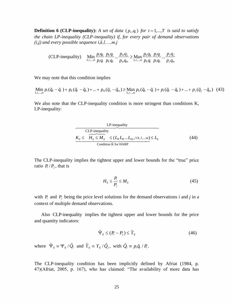
Definition 6 (CLP-inequality): A set of data ( , )t tp q for 1,...,t T is said to satisfy

the chain LP-inequality (CLP-inequality) if, for every pair of demand observations

(i,j) and every possible sequence i,k,l,…,m,j

(CLP-inequality) , ,..., , ,...,

Min ... Max ...m j j ji k k l k k l l

k l m k l mi i k k m m k i l k j m

p q p qp q p q p q p q

p q p q p q p q p q p q

We may note that this condition implies

, ,..., , ,...,Min ( ) ( ) ... ( ) Max ( ) ( ) ... ( )i k i k l k m j m k k i l l k j j mk l m k l m

p q q p q q p q q p q q p q q p q q (43)

We also note that the CLP-inequality condition is more stringent than conditions K,

LP-inequality:

Condition K for HARP

, , ...

LP-inequality

CLP-inequality

( ... , )ij ij ij ik kl mj ijk l mK H M L L L L

(44)

The CLP-inequality implies the tightest upper and lower bounds for the “true” price

ratio /i jP P , that is

i

ij ij

j

PH M

P (45)

with iP and jP being the price level solutions for the demand observations i and j in a

context of multiple demand observations.

Also CLP-inequality implies the tightest upper and lower bounds for the price

and quantity indicators:

( )ij i j ijP P (46)

where /ij ij iQ and /ij ij jQ , with /t t t tQ p q P .

The CLP-inequality condition has been implicitly defined by Afriat (1984, p.

47)(Afriat, 2005, p. 167), who has claimed: “The availability of more data has

26

removed some indeterminacy and narrowed the limits. These numbers [i.e. the

traditional bilateral Laspeyres index numbers] can fall outside limits now effective,

and then they are not true indices themselves, unlike the Laspeyres index for two

isolated periods. The new limits are obtained by a generalized formulae or algorithm

involving all the data simultaneously, unlike the Laspeyres and all price index

formulae of the type recognized by Fisher. The result is not even conventionally

algebraical in the way usually required for a price index.” 9

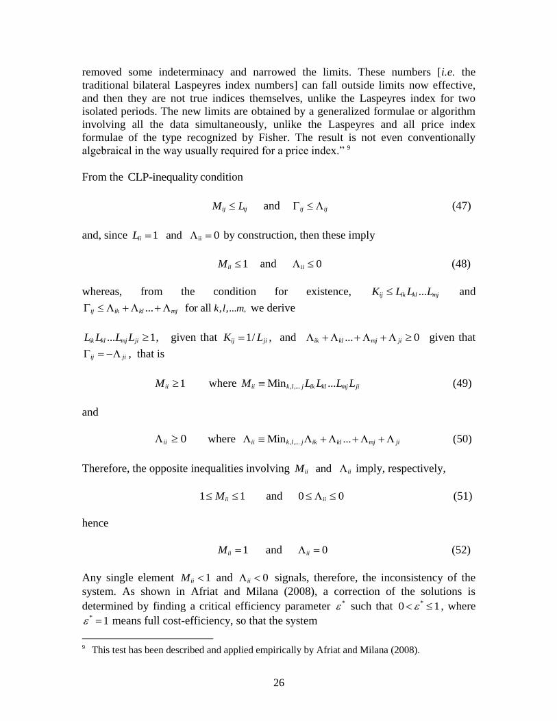
From the CLP-inequality condition

ij ijM L and ij ij (47)

and, since ii1 and 0iiL by construction, then these imply

1iiM and ii 0 (48)

whereas, from the condition for existence, ...ij ik kl mjK L L L and

,, ,...... for all ij ik kl mj k l m we derive

... 1ik kl mj jiL L L L , given that 1/ij jiK L , and ... 0ik kl mj ji given that

ij ji , that is

1iiM where , ,...Min ...ii k l j ik kl mj jiM L L L L (49)

and

0ii where , ,...Min ...ii k l j ik kl mj ji (50)

Therefore, the opposite inequalities involving and ii iiM imply, respectively,

1 1iiM and 0 0ii (51)

hence

1iiM and 0ii (52)

Any single element 1iiM and 0ii signals, therefore, the inconsistency of the

system. As shown in Afriat and Milana (2008), a correction of the solutions is

determined by finding a critical efficiency parameter * such that *0 1 , where * 1 means full cost-efficiency, so that the system

9 This test has been described and applied empirically by Afriat and Milana (2008).

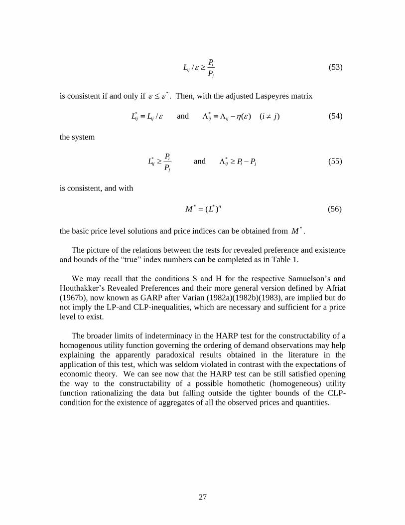
27

/i

ij

j

PL

P (53)

is consistent if and only if * . Then, with the adjusted Laspeyres matrix

* /ij ijL L and * ( )ij ij ( )i j (54)

the system

* iij

j

PL

P and *

ij i jP P (55)

is consistent, and with

* *( )nM L (56)

the basic price level solutions and price indices can be obtained from *M .

The picture of the relations between the tests for revealed preference and existence

and bounds of the “true” index numbers can be completed as in Table 1.

We may recall that the conditions S and H for the respective Samuelson‟s and

Houthakker‟s Revealed Preferences and their more general version defined by Afriat

(1967b), now known as GARP after Varian (1982a)(1982b)(1983), are implied but do

not imply the LP-and CLP-inequalities, which are necessary and sufficient for a price

level to exist.

The broader limits of indeterminacy in the HARP test for the constructability of a

homogenous utility function governing the ordering of demand observations may help

explaining the apparently paradoxical results obtained in the literature in the

application of this test, which was seldom violated in contrast with the expectations of

economic theory. We can see now that the HARP test can be still satisfied opening

the way to the constructability of a possible homothetic (homogeneous) utility

function rationalizing the data but falling outside the tighter bounds of the CLP-

condition for the existence of aggregates of all the observed prices and quantities.

28

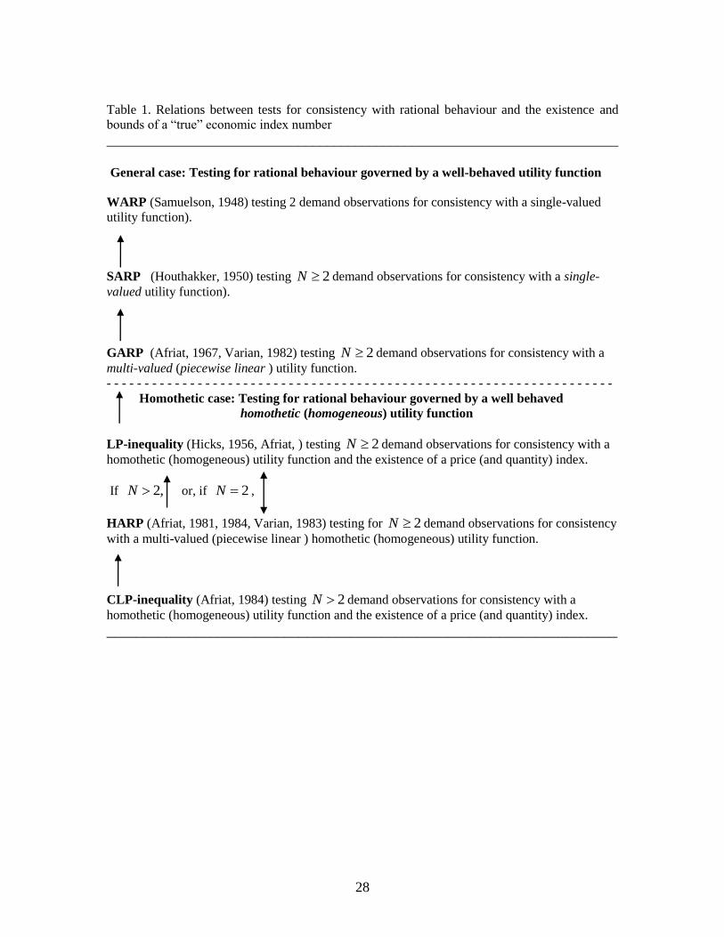
Table 1. Relations between tests for consistency with rational behaviour and the existence and

bounds of a “true” economic index number

________________________________________________________________________

General case: Testing for rational behaviour governed by a well-behaved utility function

WARP (Samuelson, 1948) testing 2 demand observations for consistency with a single-valued

utility function).

SARP (Houthakker, 1950) testing 2N demand observations for consistency with a single-

valued utility function).

GARP (Afriat, 1967, Varian, 1982) testing 2N demand observations for consistency with a

multi-valued (piecewise linear ) utility function.

- - - - - - - - - - - - - - - - - - - - - - - - - - - - - - - - - - - - - - - - - - - - - - - - - - - - - - - - - - - - - - - - - - -

Homothetic case: Testing for rational behaviour governed by a well behaved

homothetic (homogeneous) utility function

LP-inequality (Hicks, 1956, Afriat, ) testing 2N demand observations for consistency with a

homothetic (homogeneous) utility function and the existence of a price (and quantity) index.

If 2,N or, if 2N ,

HARP (Afriat, 1981, 1984, Varian, 1983) testing for 2N demand observations for consistency

with a multi-valued (piecewise linear ) homothetic (homogeneous) utility function.

CLP-inequality (Afriat, 1984) testing 2N demand observations for consistency with a

homothetic (homogeneous) utility function and the existence of a price (and quantity) index.

_____________________________________________________________________

29

Moreover, the system of inequalities

1

ij ij

ji

M PH

for every i,j (26)

where

i

ij

j

PP

P for every i,j

has solutions in terms of price levels. Analogously, the system of inequalities

ij ji ij for every i,j (27)

where

ij i jP P for every i,j

has the same solutions in price levels. The price level tP can be interpreted as values

of the aggregator price function

( )t tP e p every i,j (28)

where e(p) is the “true” aggregator function of prices.

Accordingly, the system of inequalities

1 i

ij

ji j

PH

M P for every i,j (32)

has solutions that may be interpreted in terms of price levels. Analogously, the

system of inequalities

( )ij ij i jP P for every i,j (33)

has the same solutions in price levels.

There remains, however, a certain degree of indeterminacy regarding the

aggregate price levels. While the “true” measure remains unknown, we have tight

upper and lower bounds of its possible values. The remaining question regards the

transitivity requirement. In both matrices M and H we have noticed the triangular

30

inequalities it tj ijM M M and it tj ijH H H for every i,j, and t. By contrast, any true

aggregate economic measure defined in terms of ratios or differences and its bounds

should be transitive, so that it tj ijP P P and it tj ij .

In the general case, while remaining in a range of indeterminacy, we can calculate

alternative bounds of price index numbers and indicators using the tight upper and

lower level solutions. If, without any loss of generality, the aggregate price levels are

assumed to be normalized so that 1 1,P then

1 1max / = max i t it t t it tP M M M H

for all i‟s (57)

1 1max ( ) max ( )i it t it t

for all i‟s (57‟)

where iP

= ( )e p

with

( ) inf : ( ); / ( ) for all t t t t txe p px p x e p x q f q t

being the “over-cost” aggregator function of price levels.

Analogously,

1 1min / mini t it t t it tP H H H M

for all i‟s (58)

1 1min ( ) min ( )i t it t t it tM

for all i‟s (58‟)

where iP

( )e p

with

( ) sup : ( ); / ( ) for all t t t t txe p px p x e p x q f q t

(36)

being the “under-cost” aggregator function of price levels.

The “over-cost” and “under-cost” aggregators of prices ( )e p

and ( )e p

are concave

conical functions which have polyhedral and polytope forms, respectively. They are

conjugate dual to “under-cost” and “over-cost” aggregators of

quantities ( ) / ( )f q p q e p

and ( ) . / ( )f q p q e p

that are concave conical functions

with polytope and polyhedral forms, respectively. These functions are such that

( )e p

( )e p

and ( )f q

( )f q

.

The chain-consistent bounds of aggregate price measure are therefore obtained as

/ij i jP P P

and ij i j

for every i,j (59)

31

/ij i jP P P

and ij i j

for every i,j (60)

The price index numbers defined in terms of ratios satisfy all Fisher’s tests:

1iiP

and 1iiP

for every i Identity test

ijP

and ijP

if i jp p General mean of price relatives test

(linear homogeneity in price levels) from which the identity test can be derived as a special case with 1)

1ij jiP P

and 1ij jiP P

for every ,i j Time-reversal test

ij jk ikP P P

and ij jk ikP P P

for every , ,i j k Chain (or Circular-reversal) test

*ij ijP P

and *ij ijP P

where *t tp p and * /t tq q for ,t i j

Dimensional invariance test

/ij ij i jP Q E E

and /ij ij i jP Q E E

for every i,j (Weak) factor-reversal test10

Fisher‟s tests, originally defined for index numbers in terms of ratios, are equivalent

to the following tests, valid for indicators in terms of differences:

Identity test: 0;ii ii

General mean of price relative test:

( 1) if ;Pij Pij i jp p

Time reversal test: 0;ij ji

0;Pij Pji

Chain (or Circular reversal) test: ;ij jk ik

;ij jk ik

Dimensional

invariance test (if also prices are normalized):

*

ij ij

and *ij ij

where *t tp p and * /t tq q for ,t i j ; (Weak)

factor-reversal test: ij Qij i jE E and ij Qij i jE E

for every i,j.

This result seems to contrast the conclusions derived from Frisch‟s “impossibility

theorem” in index number theory and, more recently from those of other authors (see,

10

Samuelson and Swamy (1974, p. 575) have introduced the concept of the weak factor-reversal

test, as opposed to the strong factor-reversal test: “we drop the strong requirement that the same

formula should apply to q s to p. A man and wife should be properly matched; but that does not

mean I should marry my identical twin!”.

32

for example, Van Veelen, 2002), but is perfectly in line with Samuelson and Swamy

(1974, p. 566), who have claimed: “[a]lthough Ragnar Frisch (1930) has proved that,

when the number of goods exceeds unity, it is impossible to find well-behaved

formulae that satisfy all of these Fisher criteria, we derive here canonical index

numbers of price and quantity that do meet the spirit of all of Fisher‟s criteria in the

only case in which a single index number of the price of cost of living makes

economic sense―namely, the (“homothetic”) case of unitary income elasticities in

which at all levels of living the calculated price change is the same. This seeming

contradiction with Frisch is possible because the price and quantity variables are not

here allowed to be arbitrary independent variables, but rather are constrained to

satisfy the observable demand functions which optimize well-being” (emphasis in the

original text).

In the practical case, we cannot deal with the single “true” index number just

because this remains unknown, but we can construct two bounds (the tightest upper

and lower bounds) of the closed set of possible numerical values of this index

number, if the conditions of its existence are satisfied. The toll we pay for satisfying

all Fisher‟s tests and overcome the “impossibility theorem” is to deal with two bound

estimates rather then an “ideal” single measure, which ends unavoidably to fail to

satisfy at least one of those requirements.

Afriat‟s method is to find whether a well behaved utility function can be

reconstructed that is consistent with the finite set of observed choices satisfying

GARP. However, this utility is not unique. There are generally other utility functions

and the recoverability problem becomes how to reconstruct the entire set of these

utility functions that would fit the observed data simultaneously.

For any given 0q , there is the set of 'sq that are revealed preferred to 0q 0( ( ))RP q

and set of 'sq that are revealed worse than 0q 0( ( )).RW q A simple example is given

in Figure 1. The area corresponding to the set of possible utility functions which

satisy GARP is that which does not belong to 0( )RP q and 0( ).RW q

The necessary and sufficient condition for the existence of a price and quantity

aggregate measure is that the observed data are consistent with homothetic

preferences. Following Keynes‟ (1930, pp. 105-106) “method of limits”, as re-

exposed by Afriat (1977, pp. 108-115), we may ask whether it is possible to identify

the area corresponding to the set of money metric utility functions passing through the

reference point. The same observations considered in Figure 1 are shown in Figure 2,

where this area is restricted between the upper and lower bounds of the value of the

expenditure function passing through the point 0q . These bounds are obtained by

inflating the base value of the expenditure function by means of the Laspeyres and

Paasche price indexes, respectively. We may note that these bounds are generally

tighter than the limits represented with revealed-preference methods (as shown in

Fugure 1).

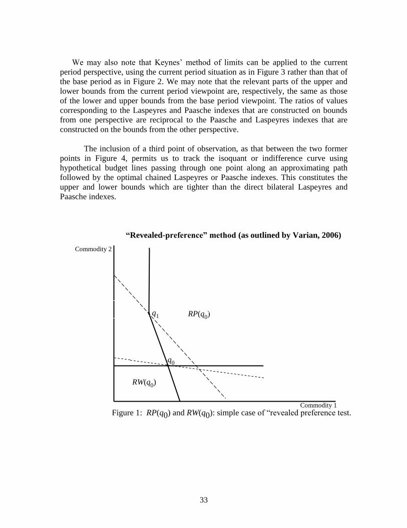
33

We may also note that Keynes‟ method of limits can be applied to the current

period perspective, using the current period situation as in Figure 3 rather than that of

the base period as in Figure 2. We may note that the relevant parts of the upper and

lower bounds from the current period viewpoint are, respectively, the same as those

of the lower and upper bounds from the base period viewpoint. The ratios of values

corresponding to the Laspeyres and Paasche indexes that are constructed on bounds

from one perspective are reciprocal to the Paasche and Laspeyres indexes that are

constructed on the bounds from the other perspective.

The inclusion of a third point of observation, as that between the two former

points in Figure 4, permits us to track the isoquant or indifference curve using

hypothetical budget lines passing through one point along an approximating path

followed by the optimal chained Laspeyres or Paasche indexes. This constitutes the

upper and lower bounds which are tighter than the direct bilateral Laspeyres and

Paasche indexes.

“Revealed-preference” method (as outlined by Varian, 2006)

Figure 1: RP(q0) and RW(q0): simple case of “revealed preference test.

Commodity 2

....

RP(q0)

)

RW(q0)

q1

q0

Commodity 1

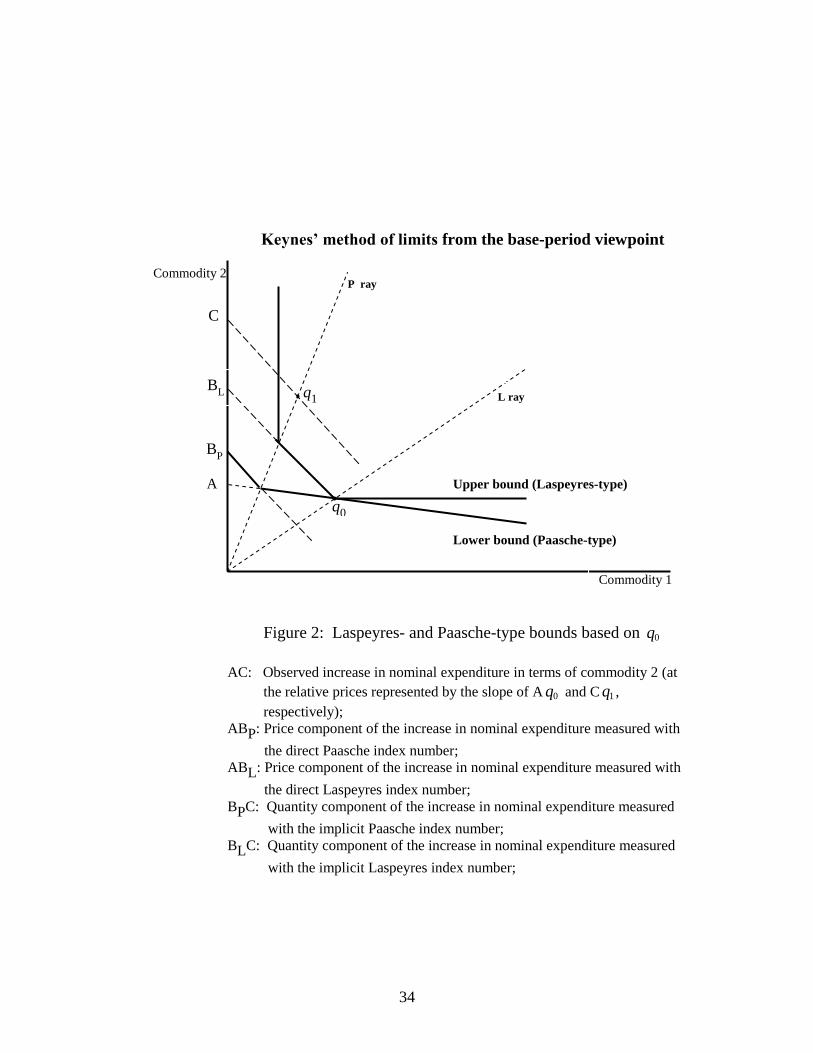
34

Keynes’ method of limits from the base-period viewpoint

Figure 2: Laspeyres- and Paasche-type bounds based on 0q

AC: Observed increase in nominal expenditure in terms of commodity 2 (at

the relative prices represented by the slope of A 0q and C 1q ,

respectively);

ABP: Price component of the increase in nominal expenditure measured with

the direct Paasche index number;

ABL: Price component of the increase in nominal expenditure measured with

the direct Laspeyres index number;

BPC: Quantity component of the increase in nominal expenditure measured

with the implicit Paasche index number;

BLC: Quantity component of the increase in nominal expenditure measured

with the implicit Laspeyres index number;

Upper bound (Laspeyres-type)

Lower bound (Paasche-type)

....A

C

BP

BL

P ray

L ray q1

q0

Commodity 2

Commodity 1

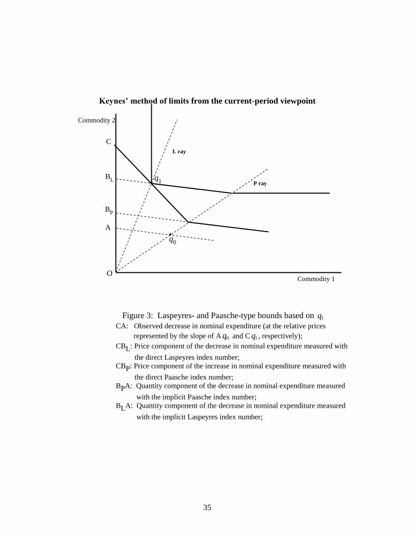
35

Keynes’ method of limits from the current-period viewpoint

Figure 3: Laspeyres- and Paasche-type bounds based on 1q

CA: Observed decrease in nominal expenditure (at the relative prices

represented by the slope of A 0q and C 1q , respectively);

CBL: Price component of the decrease in nominal expenditure measured with

the direct Laspeyres index number;

CBP: Price component of the increase in nominal expenditure measured with

the direct Paasche index number;

BPA: Quantity component of the decrease in nominal expenditure measured

with the implicit Paasche index number;

BLA: Quantity component of the decrease in nominal expenditure measured

with the implicit Laspeyres index number;

L ray

....A

BP

BL

C

q0

P ray

Commodity 2

Commodity 1

q1

O

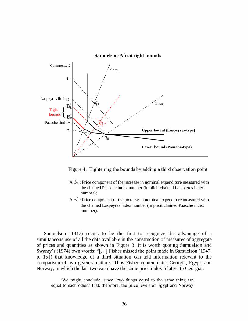
36

Samuelson-Afriat tight bounds

Figure 4: Tightening the bounds by adding a third observation point

A*PB : Price component of the increase in nominal expenditure measured with

the chained Paasche index number (implicit chained Laspyeres index

number);

A*LB : Price component of the increase in nominal expenditure measured with

the chained Laspeyres index number (implicit chained Paasche index

number).

Samuelson (1947) seems to be the first to recognize the advantage of a

simultaneous use of all the data available in the construction of measures of aggregate

of prices and quantities as shown in Figure 3. It is worth quoting Samuelson and

Swamy‟s (1974) own words: “[…] Fisher missed the point made in Samuelson (1947,

p. 151) that knowledge of a third situation can add information relevant to the

comparison of two given situations. Thus Fisher contemplates Georgia, Egypt, and

Norway, in which the last two each have the same price index relative to Georgia :

“„We might conclude, since „two things equal to the same thing are

equal to each other,‟ that, therefore, the price levels of Egypt and Norway

Upper bound (Laspeyres-type)

Lower bound (Paasche-type)

Commodity 2

Paasche limit

Laspeyres limit

P ray

L ray

Tight

bounds

....A

C

PB

BL q1

q0

q2

*LB

*PB

37

must equal, and this would be the case if we compare Egypt and Norway

via Georgia. But, evidently, if we are intent on getting the very best

comparison between Norway, we shall not go to Georgia for our weights …

[which are], so to speak, none of Georgia‟s business.‟ [1922, p. 272].

“This simply throws away the transitivity of indifference and has been led astray by

Fisher‟s unwarranted belief that only fixed-weights lead to the circular‟s test‟s being

satisfied (an assertion contradicted by our /i jP P and /i jQ Q forms.”

One of Afriat‟s main contribution in index number theory has been the

development an original approach of constructing aggregating index numbers using

all the data simultaneously (see Afriat, 1967, 1981, 1984, 2005). He also has

developed an efficient algorithm to find the minimum path of chained upper limit

index numbers (the Laspeyres indices on the demand side). In the following section

this algorithm is briefly described.

4. The Afriat’s power algorithm

With any chain of series of observation points , , ,..., , ,i k l m j there is the associated

Laspeyres chain product ... .ik kl mjL L L A simple chain among n elements is one without

repeated elements, or loops. There are

( 1)...( 1) !/ !n n n r n r

simple chains of length r n and, therefore, altogether the finite number

![1 1/1! 1/ 2! ... 1/( 1)!]n n

Finding the optimal path efficiently among this number of possible chains becomes a

computation problem as the number of elements increases. A way find this optimal

path is to note that Hicks (1956)-Afriat (1977) LP inequality condition for the

existence of the “true” aggregating index number is given by ij ijK L , that is the

Paasche index does not exceed the Laspeyres index. This is is equivalent to the Afriat

(1977) equivalent test

1ij jiL L (61)

Another way of stating this condition is that the 2 2 L-matrix

12

21

1

1

LL

L

38

be idempotent, that is L L L , in a modified arithmetic where + means min. In a

series of theorems, Afriat has shown that also in the general case

( )nM L where 2n (62)

with raising the n n -order matrix L of bilateral upper limit indexes to the power n

is made in a modified arithmetic where + means min.

In a series of theorems, Afriat has shown that the existence of a solution

...

min ...ij ik kl mjkl m

M L L L where 1iiM (63)

is a necessary and sufficient test for reaching the minimum cycle satisfying the

aggregation condition represented by the chained LP-inequality ij ijH M for every

i,j.

A similar procedure can be applied to the lower bound indexes (the Paasche

indexes on the demand side), where the matrix of these bilateral indexes is raised to

the power n in a modified arithmetic where + means max. The solution

...

max ...ij ik kl mjkl m

H K K K

...

1 1 1 1max ...kl m

ki lk jm jiL L L M where 1iiH (64)

is also a necessary and sufficient simultaneous test for reaching the minimum cycle

satisfying the aggregation condition, that is ij ijH M (the chained LP-inequality).

Diagonal elements 1iiM and 1iiH tell the inconsistency of the system. A

critical efficiency parameter * can be found for correction of the L matrix as

described in the former section. For any element 1iiM , determine the number id

of nodes in the path ...i i and

1

( ) idi iie M (65)

If 1iiM , give ie the value of 1 (that is 1ie ) and then the critical efficiency

parameter is determined as

* mini i (66)

The adjusted Laspeyres matrix is obtained as

39

* */L L (67)

and the procedure goes on as before with *L in place of the original L.

5. Multifactor productivity measurement

The methodology outlined above can be applied to the measurement of price and

quantity aggregates in the analysis of production activities. The economic theory of

production is isomorphic to the economic theory of consumption (see Samuelson,

1950, Samuelson and Swamy, 1974, p. 588, Muellbauer, 1971a, 1971b, Fisher and

Shell, 1972, 1998, Diewert, 1983, and Fisher, 1995). In the theory of output supply,

the only difference with the theory of input demand is that convexity leads to

maximization where concavity leads to minimization and all bounds are reversed.

An invariant index numbers of output, input, and productivity can be constructed if

the necessary and sufficient chain-consistent Laspeyres-Paasche inequality condition

is satisfied. A data set giving account of all outputs and inputs is most likely to be

consistent with this condition. A convenient way is to consider the accounting

equations of nominal value of net profits:

t yt t t tp y w x (68)

where yp and y are the price and quantities of outputs and w and x are the prices and

quantities of inputs. If the set of outputs and inputs is complete, we might expect that

the conditions of aggregation of input and output quantities are fulfilled. In this case

the CLP-inequality condition should be satisfied. Following Samuelson (1950, p. 23)

and Debreu (1959, p. 38), we might consider inputs as negative outputs and convert

the foregoing accounting equation in the form

t t tp q (69)

where [ ]yp p w and [ - ]q y x . By applying the definitions and

methodology outlined in the previous section, we could calculate the bounds of the

price and quantity indexes between two situations:

ij ij ij ij ijP Q P Q

(70)

where

iij

j

,

iij

j

PP

P

, i

ij

j

QQ

Q

, i

ij

j

PP

P

, i

ij

j

QQ

Q

40

with ijP

, ijP

, ijQ

, and ijQ

have been defined in the previous section as the tight

chain-consistent upper and lower bounds of prices and quantities, respectively. As

already stated, for outputs the upper bounds are given by Paasche index numbers,

whereas the lower bounds are given by Laspeyres index numbers, that is

ij ijP P

(71)

ij ijQ Q

(72)

If these conditions are fulfilled, we could apply the Shephard-Afriat‟s factorization

theorem and redefine

( ). ( )t t tP p Q q (73)

where ( ) P p and ( )Q q are the “true” aggregator functions of prices and quantities

respectively. The chain-consistent index numbers could be calculated by following

the methodology outlined in the previous section.

On difficulty in constructing price and quantity indexes of net profits is that in the

long run equilibrium in competitive markets, there have null numerical values. Any

index number defined as a ratio where the null net profits enter in the denominator

become indeterminate. This problem has made the economic measurements of

productivity based on decomposition of net profits a “road less travelled” in the

empirical literature (the few exceptions include Archibald, 1977, Balk, 1998 and

Diewert, 2000). However, as it has been stressed in Färe and Primont (1995, p. 149)

and Milana (2006), the accounting for net profits may turn the analytical framework

much wider than that based on the analysis of revenues (gross profits) and costs of

production. Among other things, this could allow us to take into account of possible

“hidden” inputs or outputs, which may be the cause of non-constant returns to scale

and non-zero net profits.

The analysis of changes in net profits could be carried out in terms of first

differences rather than ratios (see Diewert, 2000, 2005 for a previous definition). If

we normalize the net profits by the nominal value of one output, say output 1, we get

normalized net profits. The first differences of the values taken by these normalized

net profits in two observation points i and j can be decomposed as follows

( ) ( )i j i i j i j jp q q p p q (74)

Paasche-type Laspeyres-type

quantity price

component component

41

or, alternatively,

( ) ( )i j j i j i j ip q q p p q (75)

Laspeyres-type Paasche-type

quantity price

component component

where 1 1/t t t tp q , 1( ) ( ) /t t tP p P p p , with 1/t t tp p p 1( ) ( ) /t t tQ q Q q q

with 1/t t tq q q .

The following remarks can be made regarding the foregoing decomposition

procedures11:

Remark no. 1: The two alternative decompositions offer upper and lower bounds in

the typical direct bilateral comparison.

Remark no. 2: The direct bilateral comparisons do not satisfy, in general, the

circularity test of the price and quantity components (except in the very special case

where the data are consistent with given fixed weights). We may apply the optimized

chaining procedure outlined in the previous section in order to define chain consistent

tight bounds.

Remark no. 3: Using normalized prices and quantities, the price component has the

meaning of relative multifactor productivity change distributed among changes in real

rewards of factor inputs, whereas the quantity component has the meaning of relative

change in multifactor productivity originated from changes in average productivity of

factor inputs .

A very simple example will illustrate Remark no. 3. In a stylized model of one output

(y) and one input (x) of a producer facing competitive markets, the Paasche-type

quantity component defined above becomes

( )i i jp q q 1 1ji i i

i i i j

xw x w

p y p y

j i j j ii i i

i i j i j i

x y x y xw x w

p y y p y y

11

Diewert (2000)(2005) considers the Bennet-type decomposition constructed as an arithmetic

mean of these two alternative decompositions. For the purposes of our methodology, we shall

disregard this third procedure.

42

/j i j j ii

i i j i

y y x y xw

p x y x

,i j j i

j i

y x y x

y x

since, in a competitive equilibrium, i i

i i

w y

p x

/j ji

i j j

y yy

x x x

Laspeyres-type rate of change in

productivity (76)

Similarly, by defining a Laspeyres-type technical change component, we obtain

( )j i jp q q = 1 1j j ji

i j j j

w x wx

y p y p

i j j i

i j

y x y x

y x

, which corresponds to a Paasche-type

rate of change in productivity. This result leads us to the useful result that, starting from

profit accounts, we can calculate the index number of productivity by simply adding 1 to

the foregoing formula, that is

/ ( ) 1ji

i i j

i j

yyp q q

x x (77)

6. An application to EU KLEMS data

The method of chain-consistent index numbers is ideally designed for multilateral

comparisons both at an intertemporal and interspatial context. It seems to be the only

index number method that fulfils the circularity requirement and other important

conditions for economic index numbers. The EU KLEMS database on productivity

and economic growth at industry level recently constructed by a consortium of

institutions of more than 16 countries in a EU funded research project is particularly

suitable for the application of this method12.

Interspatial comparisons require, in particular, information concerning relative

levels of prices, the Purchasing Power Parities (PPP) and/or quantities across the

examined geographical units. This type of data is going to be an integral part of the

EU KLEMS project at industry level, covering more than 30 countries. At the current

stage of the construction, however, this information is only provisional and, therefore,

we have resolved to use and update the PPP data constructed in our previous works

(see, for example, Milana, 2001 and Fujikawa and Milana, 1996a, 1996b).

We consider a subset of 10 countries (the US, Japan, the six founding member

countries of the EEC, the UK and Spain), for which price and quantities of outputs

and inputs are available at disaggregated level for the period 1995-2005. In the EU

12

The EU KLEMS database is available for free download on the web site www.euklems.net .

43

KLEMS estimates, during this period, multifactor productivity in the overall economy

appears to have grown faster in the US, by 13 per cent, followed by the other

countries at much slower speed (France with 6.2 per cent, Germany and Netherlands

around 4-6-4.7 per cent, UK with 3.2 per cent, Japan with 2.7 per cent), whereas it has

even decreased in others (Belgium and Luxembourg with -2.6-2.7 per cent, Italy with

-4.5 per cent, and Spain with -7.5 per cent).

However, these estimates are difficult to compare both directly on a bilateral basis

and indirectly in a multilateral context. They are constructed using procedures of

aggregation of outputs and inputs across the industries that hardly satisfy the required

consistency criteria. As noted elsewhere (see for example Milana, 2006), the LP-

inequality test often fails. The obtained estimates do not have, in this case, the

legitimate meaning of aggregates. Moreover, the use of a specific index number

formula adds further difficulties since the aggregation is jointly tested with the chosen

functional form.

In the general case, the chosen index number formula does not only fail to satisfy

the transitivity requirement, but also affects the ranking of the countries‟ position.

Figures 4 and 5 show the relative levels of MFP with respect to that in the US in 1995

along a different path of chaining the upper limit (Paasche) indexes. The ranking

position of the countries changes according to the chosen path. This unwarrant result

has been already noted in previous empirical studies.

The price level solution allows us to construct the matrix of chain-consistent

“true” index numbers. Tables 3 and 4 show the resulting transitive index numbers of

multifactor productivity levels with respect to that in the US in 1995 and 2005,

respectively. These are obtained by chosing the highest and the lowest levels of MFP

levels resulting, mutatis mutandis, from the application of formulas (59) and (60).

These level estimates have been obtained after an adjustment for inefficiency. The

parameters of adjustments are given below the tables. Part of the gap in MFP levels

with respect to the reference country appears to be due to inefficiency.

The country ranking seems to be less influenced although some changes are worth

noting. For example, Belgium now appears below Italy and the Netherlands below

France, whereas they were in a reversed position in the original comparison.

We should emphasize, however, that these results are only provisional. A number

of refinements should be made on the data. In particular, the PPP data considered here

should be carefully scrutinized also in the light of the alternative estimates that will

hopefully become available in the immediate future. More countries should be added

to the set of comparisons in order to acquire further information on the technology in

use.

44

8. Conclusive remarks

Multilateral index numbers have always been considered as problematic since Irving

Fisher's (1922) rebuttal of the property of circularity. Since then, transitive measures

have been achieved either by “smoothing out” inconsistencies of bilateral

comparisons, or by extending the index number approach to some parametric

estimation of the underlying economic functions, thus resolving to simulations in

order to take into account price-induced substitution effects.

All the difficulties of constructing economic index numbers that have been

identified under the various formulations of an impossibility theorem can be

overcome by relinquishing a point estimate and accepting to deal with a (tightly)

bounded closed interval of alternative candidates of the unknown “true” measures.

However, the tighter the bounds the more useful these are for potential users of the

estimates.

The method proposed does not require that a non-observational object like a utility

or technological function governing the economic agents‟ behaviour really exists.

Rather, it only finds it convenient to test whether the observed data can be

rationalized with such theoretical functions. Assuming that these can be of general

forms including those that are multivalued (linear peace-wise), similar to the

functions used in activity analysis, we can try to find optimized chained Laspeyres

and Paasche index numbers. These should be “exact” for such functions and can be

considered as tight bounds of the interval of numerical values comprising the

unknown “true” measure. If these functions fit the observed data perfectly, then these

data may have been generated by rational behaviour and no inefficiency has occured.

A number of difficulties, however, may arise when applying the method to the

actual data. Many of these may arise from failures of the LP-inequality test in some

bilateral comparisons. This does not necessarily entails inefficiency per se. The LP-

inequality condition for the existence of an aggregating index are very clearly stated

in the demand or supply contexts, but may become somewhat indeterminate at a

macro level, where demand and supply interact with each other thus offsetting totally

or partially their opposite directions when price conditions tend to change. This is a

classical difficulty in index number theory, which arises when aggregation takes place

at various levels simultaneously (over outputs, over firms, and over all industries and

consumers).

Moreover, even in a partial equilibrium context, the solutions found in the usual

situation of inefficiency may not be univocal not only in terms of relative levels, but

also in their ranking. This is because the aggregation refers to an underlying utility or

technology function that does not fit the data perfectly, but only approximately.

Despite all these problems, the methodology applied here appears to respond

45

positively to the long-standing search for a definite answer to the “index number

problem”.

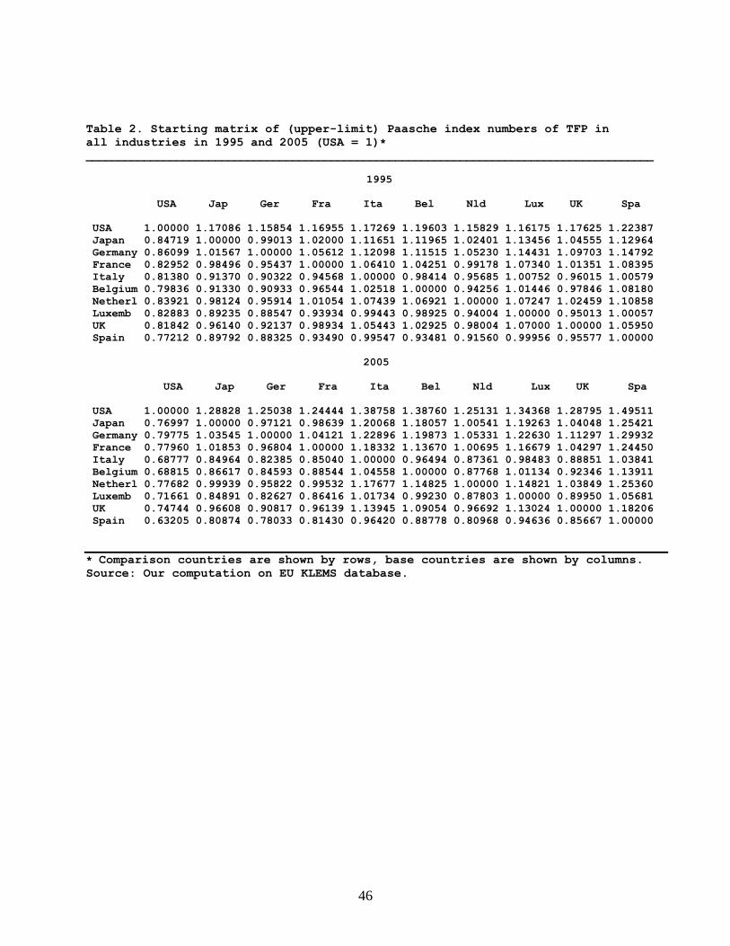
46

Table 2. Starting matrix of (upper-limit) Paasche index numbers of TFP in

all industries in 1995 and 2005 (USA = 1)* ________________________________________________________________________________________

1995

USA Jap Ger Fra Ita Bel Nld Lux UK Spa

USA 1.00000 1.17086 1.15854 1.16955 1.17269 1.19603 1.15829 1.16175 1.17625 1.22387

Japan 0.84719 1.00000 0.99013 1.02000 1.11651 1.11965 1.02401 1.13456 1.04555 1.12964

Germany 0.86099 1.01567 1.00000 1.05612 1.12098 1.11515 1.05230 1.14431 1.09703 1.14792

France 0.82952 0.98496 0.95437 1.00000 1.06410 1.04251 0.99178 1.07340 1.01351 1.08395

Italy 0.81380 0.91370 0.90322 0.94568 1.00000 0.98414 0.95685 1.00752 0.96015 1.00579

Belgium 0.79836 0.91330 0.90933 0.96544 1.02518 1.00000 0.94256 1.01446 0.97846 1.08180

Netherl 0.83921 0.98124 0.95914 1.01054 1.07439 1.06921 1.00000 1.07247 1.02459 1.10858

Luxemb 0.82883 0.89235 0.88547 0.93934 0.99443 0.98925 0.94004 1.00000 0.95013 1.00057

UK 0.81842 0.96140 0.92137 0.98934 1.05443 1.02925 0.98004 1.07000 1.00000 1.05950

Spain 0.77212 0.89792 0.88325 0.93490 0.99547 0.93481 0.91560 0.99956 0.95577 1.00000

2005

USA Jap Ger Fra Ita Bel Nld Lux UK Spa

USA 1.00000 1.28828 1.25038 1.24444 1.38758 1.38760 1.25131 1.34368 1.28795 1.49511

Japan 0.76997 1.00000 0.97121 0.98639 1.20068 1.18057 1.00541 1.19263 1.04048 1.25421

Germany 0.79775 1.03545 1.00000 1.04121 1.22896 1.19873 1.05331 1.22630 1.11297 1.29932

France 0.77960 1.01853 0.96804 1.00000 1.18332 1.13670 1.00695 1.16679 1.04297 1.24450

Italy 0.68777 0.84964 0.82385 0.85040 1.00000 0.96494 0.87361 0.98483 0.88851 1.03841

Belgium 0.68815 0.86617 0.84593 0.88544 1.04558 1.00000 0.87768 1.01134 0.92346 1.13911

Netherl 0.77682 0.99939 0.95822 0.99532 1.17677 1.14825 1.00000 1.14821 1.03849 1.25360

Luxemb 0.71661 0.84891 0.82627 0.86416 1.01734 0.99230 0.87803 1.00000 0.89950 1.05681

UK 0.74744 0.96608 0.90817 0.96139 1.13945 1.09054 0.96692 1.13024 1.00000 1.18206

Spain 0.63205 0.80874 0.78033 0.81430 0.96420 0.88778 0.80968 0.94636 0.85667 1.00000

* Comparison countries are shown by rows, base countries are shown by columns.

Source: Our computation on EU KLEMS database.

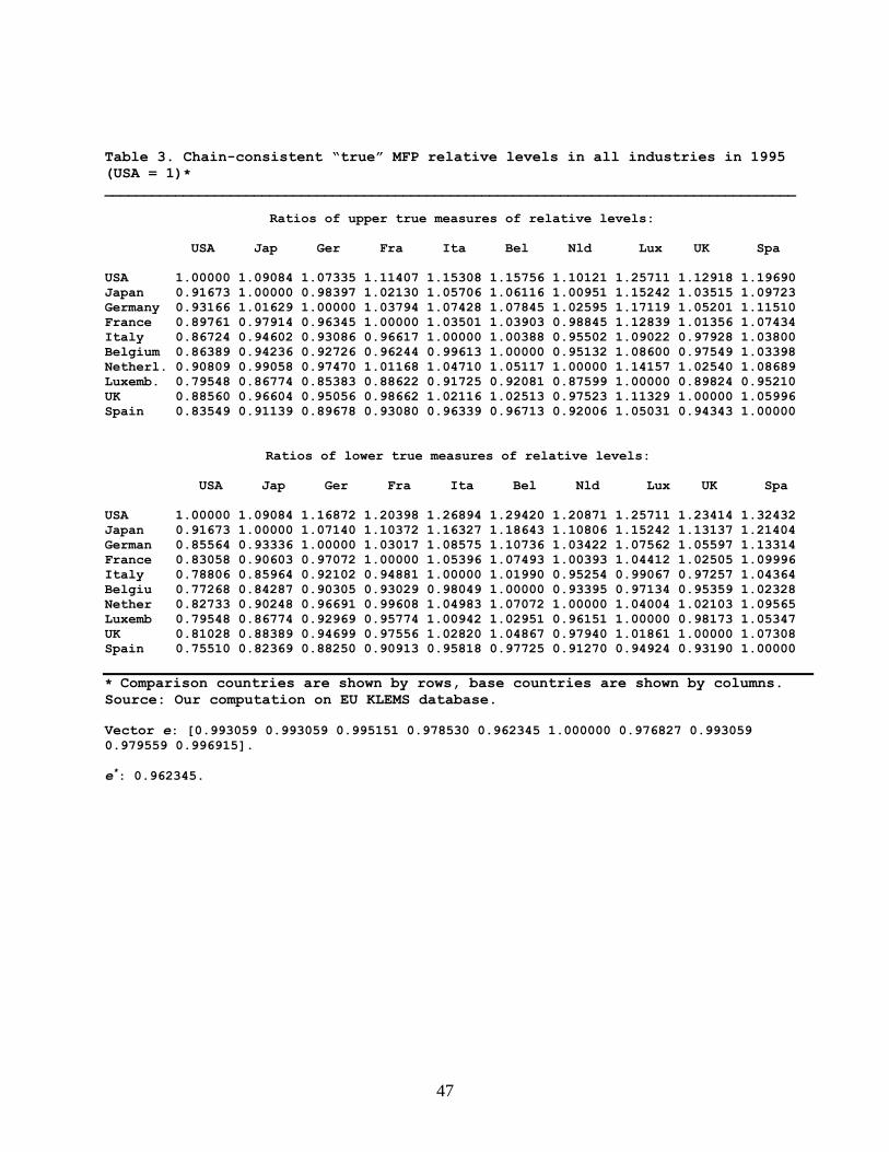
47

Table 3. Chain-consistent “true” MFP relative levels in all industries in 1995

(USA = 1)* ________________________________________________________________________________________

Ratios of upper true measures of relative levels:

USA Jap Ger Fra Ita Bel Nld Lux UK Spa

USA 1.00000 1.09084 1.07335 1.11407 1.15308 1.15756 1.10121 1.25711 1.12918 1.19690

Japan 0.91673 1.00000 0.98397 1.02130 1.05706 1.06116 1.00951 1.15242 1.03515 1.09723

Germany 0.93166 1.01629 1.00000 1.03794 1.07428 1.07845 1.02595 1.17119 1.05201 1.11510

France 0.89761 0.97914 0.96345 1.00000 1.03501 1.03903 0.98845 1.12839 1.01356 1.07434

Italy 0.86724 0.94602 0.93086 0.96617 1.00000 1.00388 0.95502 1.09022 0.97928 1.03800

Belgium 0.86389 0.94236 0.92726 0.96244 0.99613 1.00000 0.95132 1.08600 0.97549 1.03398

Netherl. 0.90809 0.99058 0.97470 1.01168 1.04710 1.05117 1.00000 1.14157 1.02540 1.08689

Luxemb. 0.79548 0.86774 0.85383 0.88622 0.91725 0.92081 0.87599 1.00000 0.89824 0.95210

UK 0.88560 0.96604 0.95056 0.98662 1.02116 1.02513 0.97523 1.11329 1.00000 1.05996

Spain 0.83549 0.91139 0.89678 0.93080 0.96339 0.96713 0.92006 1.05031 0.94343 1.00000

Ratios of lower true measures of relative levels:

USA Jap Ger Fra Ita Bel Nld Lux UK Spa

USA 1.00000 1.09084 1.16872 1.20398 1.26894 1.29420 1.20871 1.25711 1.23414 1.32432

Japan 0.91673 1.00000 1.07140 1.10372 1.16327 1.18643 1.10806 1.15242 1.13137 1.21404

German 0.85564 0.93336 1.00000 1.03017 1.08575 1.10736 1.03422 1.07562 1.05597 1.13314

France 0.83058 0.90603 0.97072 1.00000 1.05396 1.07493 1.00393 1.04412 1.02505 1.09996

Italy 0.78806 0.85964 0.92102 0.94881 1.00000 1.01990 0.95254 0.99067 0.97257 1.04364

Belgiu 0.77268 0.84287 0.90305 0.93029 0.98049 1.00000 0.93395 0.97134 0.95359 1.02328

Nether 0.82733 0.90248 0.96691 0.99608 1.04983 1.07072 1.00000 1.04004 1.02103 1.09565

Luxemb 0.79548 0.86774 0.92969 0.95774 1.00942 1.02951 0.96151 1.00000 0.98173 1.05347

UK 0.81028 0.88389 0.94699 0.97556 1.02820 1.04867 0.97940 1.01861 1.00000 1.07308

Spain 0.75510 0.82369 0.88250 0.90913 0.95818 0.97725 0.91270 0.94924 0.93190 1.00000

* Comparison countries are shown by rows, base countries are shown by columns.

Source: Our computation on EU KLEMS database.

Vector e: [0.993059 0.993059 0.995151 0.978530 0.962345 1.000000 0.976827 0.993059

0.979559 0.996915].

e*: 0.962345.

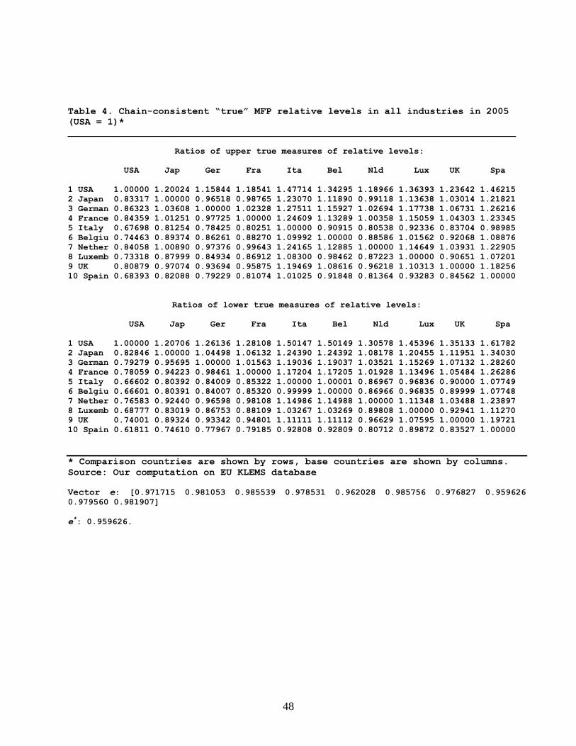
48

Table 4. Chain-consistent “true” MFP relative levels in all industries in 2005

(USA = 1)* ________________________________________________________________________________________

Ratios of upper true measures of relative levels:

USA Jap Ger Fra Ita Bel Nld Lux UK Spa

1 USA 1.00000 1.20024 1.15844 1.18541 1.47714 1.34295 1.18966 1.36393 1.23642 1.46215

2 Japan 0.83317 1.00000 0.96518 0.98765 1.23070 1.11890 0.99118 1.13638 1.03014 1.21821

3 German 0.86323 1.03608 1.00000 1.02328 1.27511 1.15927 1.02694 1.17738 1.06731 1.26216

4 France 0.84359 1.01251 0.97725 1.00000 1.24609 1.13289 1.00358 1.15059 1.04303 1.23345

5 Italy 0.67698 0.81254 0.78425 0.80251 1.00000 0.90915 0.80538 0.92336 0.83704 0.98985

6 Belgiu 0.74463 0.89374 0.86261 0.88270 1.09992 1.00000 0.88586 1.01562 0.92068 1.08876

7 Nether 0.84058 1.00890 0.97376 0.99643 1.24165 1.12885 1.00000 1.14649 1.03931 1.22905

8 Luxemb 0.73318 0.87999 0.84934 0.86912 1.08300 0.98462 0.87223 1.00000 0.90651 1.07201

9 UK 0.80879 0.97074 0.93694 0.95875 1.19469 1.08616 0.96218 1.10313 1.00000 1.18256

10 Spain 0.68393 0.82088 0.79229 0.81074 1.01025 0.91848 0.81364 0.93283 0.84562 1.00000

Ratios of lower true measures of relative levels:

USA Jap Ger Fra Ita Bel Nld Lux UK Spa

1 USA 1.00000 1.20706 1.26136 1.28108 1.50147 1.50149 1.30578 1.45396 1.35133 1.61782

2 Japan 0.82846 1.00000 1.04498 1.06132 1.24390 1.24392 1.08178 1.20455 1.11951 1.34030

3 German 0.79279 0.95695 1.00000 1.01563 1.19036 1.19037 1.03521 1.15269 1.07132 1.28260

4 France 0.78059 0.94223 0.98461 1.00000 1.17204 1.17205 1.01928 1.13496 1.05484 1.26286

5 Italy 0.66602 0.80392 0.84009 0.85322 1.00000 1.00001 0.86967 0.96836 0.90000 1.07749

6 Belgiu 0.66601 0.80391 0.84007 0.85320 0.99999 1.00000 0.86966 0.96835 0.89999 1.07748

7 Nether 0.76583 0.92440 0.96598 0.98108 1.14986 1.14988 1.00000 1.11348 1.03488 1.23897

8 Luxemb 0.68777 0.83019 0.86753 0.88109 1.03267 1.03269 0.89808 1.00000 0.92941 1.11270

9 UK 0.74001 0.89324 0.93342 0.94801 1.11111 1.11112 0.96629 1.07595 1.00000 1.19721

10 Spain 0.61811 0.74610 0.77967 0.79185 0.92808 0.92809 0.80712 0.89872 0.83527 1.00000

* Comparison countries are shown by rows, base countries are shown by columns.

Source: Our computation on EU KLEMS database

Vector e: [0.971715 0.981053 0.985539 0.978531 0.962028 0.985756 0.976827 0.959626

0.979560 0.981907]

e*: 0.959626.

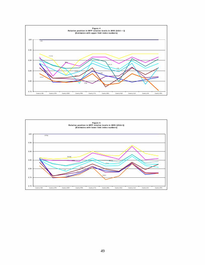
49

Figure 4

Relat ive posit ion in MFP relat ive levels in 1995 (USA = 1)

(Estimates with upper limit index numbers)

0.75

0.80

0.85

0.90

0.95

1.00

GER

JPN

NLD

UK

FRALUX

ITA

BELSPA

Countr y/ USA Countr y/ JPN Countr y/ GER Countr y/ FRA Countr y/ ITA Countr y/ BEL Countr y/ NLD Countr y/ LUX Countr y/ UK Countr y/ SPA

US

Figure 5

Relat ive posit ion in MFP relat ive levels in 1995 (USA=1)

(Estimates with lower limit index numbers)

0.70

0.75

0.80

0.85

0.90

0.95

1.00

GER

NLDJPN

FRA

UK

ITA

BEL

LUX SPA

USA

Countr y/ USA Countr y/ JPN Countr y/ GER Countr y/ FRA Countr y/ ITA Countr y/ BEL Countr y/ NLD Countr y/ LUX Countr y/ UK Countr y/ SPA

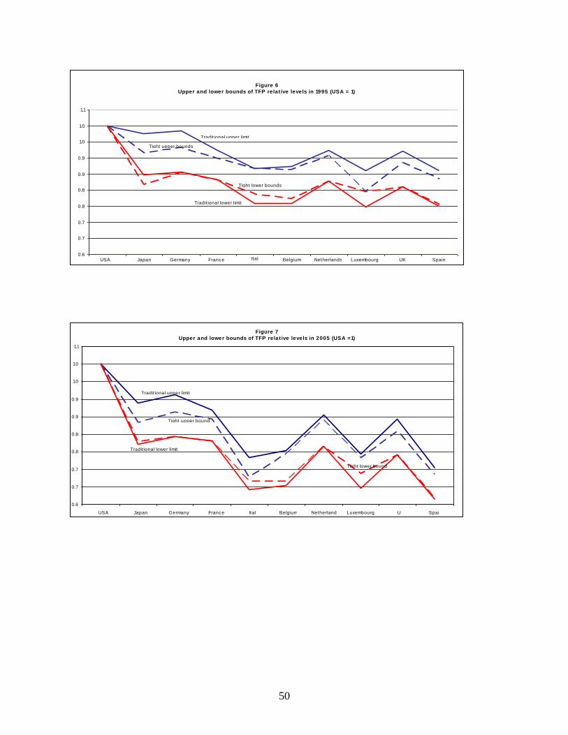
50

Figure 6

Upper and lower bounds of TFP relat ive levels in 1995 (USA = 1)

0.6

0.7

0.7

0.8

0.8

0.9

0.9

1.0

1.0

1.1

USA Japan Germany France Ital

yBelgium Netherlands Luxembourg UK Spain

Tradit ional upper limit

Tradit ional lower limit

Tight upper bounds

Tight lower bounds

Figure 7

Upper and lower bounds of TFP relat ive levels in 2005 (USA =1)

0.6

0.7

0.7

0.8

0.8

0.9

0.9

1.0

1.0

1.1

USA Japan Germany France Ital

y

Belgium Netherland

s

Spai

n

Luxembourg U

K

Tradit ional upper limit

Tradit ional lower limit

Tight upper bound

Tight lower bound

51

References

Afriat, S. N. (1953-56). Theory of Economic Index Numbers. The Consistency Condition

and Other Concepts in the Theory of Value and Demand. The Calculation of

Index Numbers of the Standard and Cost of Living. On Index Numbers in the

Theory of Value and Demand. Research Reports (mimeo.), Department of

Applied Economics, Cambridge.

Afriat, S. N. (1959). Value and Expenditure. Research Memorandum No. 7 (February),

Econometric Research Program, Princeton University.

Afriat, S. N. (1967a). The Cost of Living Index. In Martin Shubik (ed.), Studies in

Mathematical Economics in Honor of Oscar Morgenstern. Princeton University

Press.

Afriat, S. N. (1967b), “The Construction of Utility Functions from Expenditure Data”,

International Economic Review 8: 67-77.

Afriat, S. N. (1971a). The Output Limit Function in General and Convex Programming

and the Theory of Production. Econometrica 39, 309-39.

Afriat, S.N. (1972), “The Theory of International Comparisons of Real Income and

Prices”, In In D. J. Daly (ed. by), International Comparisons of Price and

Output, Studies in Income & Wealth, No.37, National Bureau of Economic

Research, New York: Columbia University Press, pp. 208-216.

Afriat, S.N. (1977), The Price Index, Cambridge, UK: Cambridge University Press.

Afriat, S. N. (1981), “On the Constructability of Consistent Price Indices Between

Several Periods Simultaneously”, in Angus Deaton (ed. by), Essays in the

Theory and Measurement of Consumer Behaviour: in Honour of Sir Richard

Stone, Cambridge, UK: Cambridge University Press, 133-161.

Afriat, S. N. (1984), “The True Index”, in A. Ingham and A.M. Ulph (eds.), Demand,

Equilibrium and Trade: Essays in Honor of Ivor F. Pearce. London: Macmillan,

37-56. Reproduced in S. N. Afriat, The Price Index and Its Extension: A chapter

in economic measurement, London and New York: Routledge, 2005, pp. 157-173.

Afriat, S.N. (2005). The Price Index and Its Extension. A Chapter in Economic

Measurement. London and New York: Routledge.

Afriat, S. N. and Nuri T. Jazairi (1988). Fisher‟s Test Approach to Index Numbers. In

Samuel Kotz and Norman L. Johnson (eds.), Encyclopedia of Statistical Sciences.

New York: John Wiley & Sons.

52

Afriat, S.N. and Milana (2008), Economics and the Price Index. London and New

York: Routledge.

Allen, Robert C. and Erwin W. Diewert (1981), “Direct Versus Implicit Superlative

Indexe Number Formulae”, Review of Economics and Statistics 63: 430-435.

Antonelli, G.B. (1886), Sulla teoria matematica dell’economia pura. Reprinted in

Giornale degli Economisti 10 (1951): 233-263.

Archibald, R. (1975), “On the Theory of Industrial Price Measurement: Input Price

Indexes”, Annals of Economic and Social Measurement 6: 57-72.

Balk, Bert M. (1998), Industrial Price, Quantity, and Productivity Indices. The Micro-

Economic Theory and An Application, Boston, Dordrecht, London, Kluwer

Academic Publishers.

Blundell, Richard (2005). How Revealing is Revealed Preference? European

Economic Journal 3, 211-35.

Blundell, Richard W., Martin Browning and Ian A. Crawford (2003). Nonparametric

Engel Curves and Revealed Preferences. Econometrica 71, 208-40.

Caves, Douglas W.; Laurits R. Christensen; and W. Erwin Diewert (1982a), "The

Economic Theory of Index Numbers and the Measurement of Input, Output,

and Productivity, Econometrica 50: 1393-1414.

Caves, Douglas W.; Laurits R. Christensen; and W. Erwin Diewert (1982b),

“Multilateral Comparisons of Output, Input, and Productivity Using

Superlative Index Numbers”, Economic Journal 92: 73-86.

Chavas, Jean-Paul and Thomas L. Cox (1990), “A Non-Parametric Analysis of

Productivity: The Case of U.S. and Japanese Manufacturing”, American

Economic Review 803, 450-64.

Chavas, J.-P. and T. Cox (1992). A Nonparametric Analysis of the Influence of Research

on Agricultural Productivity, American Journal of Agricultural Economics, 74(3),

583-91.

Chavas, J.-P. and T. Cox (1994). A Primal-Dual Approach to Nonparametric Productivity

Analysis: The Case of U.S. Agriculture. Journal of Productivity Analysis 5, 359-73.

Chavas, J.-P., M. Aliber and T. I. Cox (1994). A Nonparametric Analysis of the Source

and Nature of Technical Change: The Case of U.S. Agriculture. University of

Wisconsin-Madison, Department of Agricultural Economics, Staff Paper Series No.

373.

53

Cox, Thomas L. and Chavas, Jean-Paul (1990), “A Nonparametric Analysis of

Productivity: The Case of US Agriculture”, European Review of Agricultural

Economics 17: 449-64.

Deaton, Angus (1986), “Demand Analysis”, in Z. Griliches and M.D. Intriligator

(eds.), Handbook of Econometrics, Vol. III, Elsevier Science Publishers BV,

New York, pp. 1767-1839.

Denny, Michael (1972), “Trade and Production Sector: An Exploration of Models of

Multi-Product Technology”, Ph. D. Dissertation, University of California at

Berkeley.

Denny, Michael (1974), "The Relationship Between Functional Forms for the

Production System", Canadian Journal of Economics 7: 21-31.

Diewert, W. Erwin (1971), "An Application of the Shephard Duality Theorem: A

Generalized Leontief Production Function", Journal of Political Economy 79:

481-507.

Diewert, W. Erwin (1976), "Exact and Superlative Index Numbers", Journal of

Econometrics 4: 115-145.

Diewert, W. Erwin (1973), “Afriat and Revealed Preference Theory”, Review of

Economic Studies 40: 419-425.

Diewert, W. Erwin (1980), “Aggregation Problems in the Measurement of Capital”,

in D. Usher (ed. by), The Measurement of Capital, Studies in Income and

Wealth, Vol. 45, National Bureau of Economic Research, Chicago, University

of Chicago Press, pp. 433-528.

Diewert, W. Erwin and Celik Parkan (1983), “Linear Programming Tests of

Regularity Conditions for Production Functions”, in Quantitative Studies on

Production and Prices. Würzburg-Wien: Physica-Verlag, 131-58.

Diewert, W. Erwin and Celik Parkan (1985), “Tests for Consistency of Consumer

Data”, Journal of Econometrics 30 (1-2), 127-47.

Diewert, W. Erwin (2000), “Productivity Measurement Using Differences rather than

Ratios: A Note”, Discussion Paper 2000/1, University of New South Wales,

School of Economics

Diewert, W. Erwin (2005), “Index Number Theory Using Differences Rather Than

Ratios,” University of British Columbia, Department of Economics, American

Journal of Economics and Sociology 64: 311-360.

54

Diewert, W. Erwin and Alice O. Nakamura (2003), “Index Number Concepts, Measures

and Decomposition of Productivity Growth”, Journal of Productivity Analysis 19:

127-159.

Dowrick, Steve and John Quiggin (1994). International Comparisons of Living Standards

and Tastes: A Revealed-Preference Analysis. American Economic Review 84,

332-41.

Dowrick, Steve and John Quiggin (1997). True Measures of GDP and Convergence.

American Economic Review 87 (1), 41-64.

Famulari, Melissa (1995), A Household-Based, Nonparametric Test of Demand

Theory. Review of Economics and Statistics 372-82.

Färe, Rolf and Daniel Primont (1995), Multi-Output Production and Duality: Theory and

Applications, Norwell, MA, Kluwer Academic Publishers.

Fisher, Franklin M. and Karl Shell (1972), Economic Theory of Price Indices, New

York: Academic Press.

Fisher, Franklin M. (1995), “The Production-Theoretic Measurement of Input Price

and Quantity Indices”, Journal of Econometrics 65: 155-174.

Fisher, Franklin M. (1988), "Production-Theoretic Input Price Indices and the

Measurement of Real Aggregate Input Use", in W. Eichhorn (ed. by),

Measurement in Economics, Heidelberg, Physica-Verlag, pp. 87-98.

Fisher, Franklin M. and Karl Shell (1998), Economic Analysis of Production Price

Indexes, Cambridge, UK: Cambridge University Press.

Frisch, Ragnar (1930), “Necessary and Suffient Conditions Regarding the Form of an

Index Number Which Shall Meet Certain of Fisher‟s Tests,” Journal of

American Statistical Association 25: 297-406.

Frisch, Ragnar (1936), “Annual Survey of General Economic Theory: The Problem of

Index Numbers”, Econometrica 4: 1-39.

Fujikawa, Kiyoshi and Carlo Milana (1996a), “Bilateral and Multilateral

Comparisons of Productivity in Input-Output Analysis Using Alternative

Index Numbers”, in OECD, Industry, productivity. International Comparisons

and Measurement Issues. Paris, pp. 217-241.

Fujikawa, Kiyoshi and Carlo Milana (1996b), “Direct and Indirect Components of

Producer Prices in International Comparisons”, Presented at the 1996

Conference of Pan Pacific Association of Input-Output Studies held at the

University of Nagoya, Nagoya, Japan on 9th-10th November, 1996.

55

Gorman, W.M. (1953), “Community Preference Fields”, Econometrica 21: 63-80.

Gorman, W.M. (1961), “On a Class of Preference Fields”, Metroeconomica 13: 53-

56.

Hanoch, Giora and Michael Rothschild (1972), “Testing the Assumptions of

Production Theory: A Nonparametric Approach”, Journal of Political

Economy 80 (2), 256-75.

Hicks, J.R. (1956), A Revision of Demand Theory. Oxford: The Clarendon Press.

Hill, Robert J. (1997), “A Taxonomy of Multilateral Methods for Making

International Comparisons of Prices and Quantities”, Review of Income and

Wealth 43(1): 49-69.

Hill, Robert J. (1999a), “Comparing Price Levels across Countries Using Minimum-

Spanning Trees”, Review of Economics and Statistics 81(1): 135-142.

Hill, Robert J. (1999b), “International Comparisons Using Spanning Trees”, in A.

heston and R.E. Lipsey (eds.), International and Interarea Comparisons of

Income, Output, and Prices, Studies in Income and Wealth, Volume 61,

NBER, Chicago: The University of Chicago Press.

Hill, Robert J. (2001), “Linking Countries and Regions Using Chaining Methods and

Spanning Trees”, prepared for the Joint World Bank-OECD Seminar on

Purchasing Power Parities – Recent Advances in Methods and Applications,

Washington, D.C., 30th January-2nd February, 2001.

Hill, Robert J. (2000), “Measuring Substitution Bias in International Comparisons

Based on Additive Purchasing Power Parity Methods”, European Economic

Review 44: 145-162.

Hill, Robert J. (2004), “Constructing Price Indexes across Space and Time: The Case

of the European Union”, American Economic Review 94(5): 1379-1410.

Hill, Robert J. (2006a), “Superlative Index Numbers: Not All of Them Are Super”,

Journal of Econometrics 130: 25-43.

Hill, Robert J. (2006b), “When Does Chaining reduce the Paasche-Laspeyres Spread?

An Application to Scanner Data”, Review of Income and Wealth 52: 309-325.

Houthakker, H. (1950). Revealed Preference and Utility Function. Economica, NS 17,

159-74.

56

Hulten, Charles R. (1973), “Divisia Index Numbers”, Econometrica 41: 1017-1025.

Hulten, Charles R. (2004), “The Political Economy of Price Measurement: The NAS

Report „At What Price‟ and Beyond”, Paper prepared for the CRIW

conference Price Index Concepts and Measurement, Vancouver, Canada, June

28-29, 2004.

Kadiyala, K. Rao (1972), “Production Functions and the Elasticity of Substitution”,

Southern Economic Journal 38: 281-284.

Keren, Michael and J. Weinblatt (1984), “A Geometric Approach to Real Income

Comparisons: A Comment on Samuelson‟s „Analytical Notes on International

Real-Income Measures‟”, Economic Journal 94: 258-264.

Keynes, John M. (1930), Treatise on Money, Vol. 1, The Pure Theory of Money. New

York: Harcourt Brace.

Knoblauch, Vicki (1992), “A Tight Upper Bound on the Money Metric Utility

Function”, American Economic Review 82: 660-663.

Konüs, A.A. (1924), “Problema istinovo indeksa stoimosti zhizni”, Ekonomicheskii

Byulleten Konyunkturnovo Instituta 3: 64-71. English translation: “The

Problem of the True Index of the Cost of Living”, Econometrica 7 (Jan. 1939):

10-29.

Konüs, A.A. and S.S. Byushgens (1926), "K probleme pokupatelnoi cili deneg"

(English translation of Russian title: "On the Problem of the Purchasing

Power of Money"), Voprosi Konyunkturi II(1) (supplement to the Economic

Bulletin of the Conjuncture Institute), pp. 151-172.

Koo, Anthony Y.C. (1963), “An Empirical Test of Revealed Preference Theory”,

Econometrica 31: 646-664.

Jorgenson, Dale W. and Zvi Griliches (1967), “The Explanation of Productivity

Change”, Review of Economic Studies 34: 249-283.

Jorgenson, Dale W. and Zvi Griliches (1971), “Divisia Index Numbers and

Productivity Measurement”, Review of Income and Wealth , 38: 227-229.

Lau, Lawrence J. (1973), unpublished memorandum (cited in Diewert, 1976, p. 130).

McCarthy, M. D. (1967), “Approximation of the CES Production Function: A

Comment”, International Economic Review 8: 190-192.

57

Manser, Marilyn E. and Richard McDonald (1988). An Analysis of Substitution Bias

In Measuring Inflation, Econometrica 56, 909-30.

Milana, Carlo (1993), “Numeri indici”, Enciclopedia Italiana, Institute of the Italian

Encyclopedia founded by Giovanni Treccani, Rome, 5th Appendix (1979-

1992), pp. 704-709.

Milana, Carlo (2001), “The Input-Output Structural Decomposition Analysis of

„Flexible‟ Production Systems,” in Michael L. Lahr and Erik Dientzenbacher

(eds.), Input-Output Analysis: Frontiers and Extensions, New York, Palgrave, pp.

349-80.

Milana, Carlo (2005), “The Theory of Exact and Superlative Index Numbers Revisited”,

Working paper no. 3, EU KLEMS Project (http://www.euklems.net/publications).

Milana, Carlo (2006), “A Net Profit Approach to Productivity Measurement, with an

Application to Italy”, prepared for the Workshop on productivity

Measurement, 16-18 October, 2006, Bern, Switzerland, organized jointly by

the OECD and the Swiss government.

Muellbauer, J.N.J. (1971), “The „Pure Theory of the National Output Deflator‟

Revisited”, University of Warwick, Department of Economics, Warwick

Economic Research Paper Number 16, Coventry, United Kingdom.

Muellbauer, J.N.J. (1972), “The Theory of True Input Price Indices”, University of

Warwick, Department of Economics, Warwick Economic Research Paper

Number 17, Coventry, United Kingdom.

Neary, J. Peter (2004), “Rationalizing the Penn World Table: True Multilateral

Indices for International Comparisons of Real Income”, American Economic

Review 94: 1411-1428.

Pollak, Robert A. (1971) “The Theory of Cost-of-Living Index”, mimeo, University

Of Pennsylvania, June (Published in W. E. Diewert (ed.by), Price Level

Measurement, Amsterdam, North-Holland Publ. Co., 1990, pp. 5-77.

Quiggin, John and Matthijs van Veelen (2007), “Multilateral Indices: Conflicting

Approaches?”, Review of Income and Wealth 53 (2), 372-78.

Reinsdorf, Marhall and Jack Triplett (2004), “A Review of Reviews: Ninety Years of

Professional Thinking About the Consumer price Index and How to Measure

it”, Paper prepared for the CRIW conference Price Index Concepts and

Measurement, Vancouver, Canada, June 28-29, 2004.

Russell, R. Robert (1983), “Comment on Diewert‟s „The Theory of the Cost-of-Living

58

Index and the Measurement of Welfare Change”, in W.E. Diewert and C.

Montmarquette (eds.), Price Level Measurement: Proceedings from a

Conference Sponsored by Statistics Canada, Ottawa, Minister of Supply and

Services Canada, pp. 234-239.

Russell, R. R. and M. O. Tengesdal (2001). On the Power of Non-Parametric Tests of

the Representative Consumer Hypothesis. Mimeo, University of California,

Berkely.

Russell, R. R., Robert V. Breunig and Chia-Hui Chiu (1998). Aggregation and

Econometric Analysis of Demand and Supply. In Aman Ullah and David E. A.

Giles (eds.), Handbook of Applied Economic Statistics, New York: Marcel

Dekker, Inc., 177-236.

Samuelson, Paul A. (1938a), “A Note on the Pure Theory of Consumer‟s Behaviour”,

Economica 5: 61-71.

Samuelson, Paul A. (1938b), “A Note on the Pure Theory of Consumer‟s Behaviour:

An Addendum”, Economica 5: 353-4.

Samuelson, Paul A. (1938c), “The Empirical Implications of Utility Analysis”,

Econometrica 6: 344-356.

Samuelson, Paul A. (1947), Foundations of Economic Analysis, Cambridge, Mass.:

Harvard University Press.

Samuelson, Paul A. (1948), “Consumption Theory in Terms of Revealed Preference”,

Economica 15: 243-253.

Samuelson, Paul A. (1974), “Analytical Notes on International Real-Income

Measures”, Economic Journal 84(335): 595-608.

Samuelson, Paul A. (1984), “Second Thoughts on Analytical Income Comparisons”.

Economic Journal 94: 267-278.

Samuelson, Paul A. and Subramanian Swamy (1974), “Invariant Economic Index

Numbers and Canonical Duality: Survey and Synthesis”, American Economic

Review 64(4): 566-593.

Swamy, Subramanian (1984), “Samuelson‟s Analytical Notes on International Real-

Income Measures: A Comment”, Economic Journal 94: 265-266.

Uebe, G. (1978), “On a Flexibility Theorem of Diewert”, in W. Eichhorn, R. Henn,

O. Opitz, R.W. Shephard (eds), Theory and Applications of Economic Indices,

Würzburg, Physica-Verlag, pp. 719-729.

59

Usher, Dan (1972), “Comment on „Comparative National Income of the USSR and

the United States‟ by Abram Bergson”, In D. J. Daly (ed. by), International

Comparisons of Price and Output, Studies in Income & Wealth, No.37,

National Bureau of Economic Research, New York: Columbia University

Press, pp. 208-216.

Van Veelen, Matthijs (2002), “An Impossibility Theorem Concerning Multilateral

International Comparison of Volumes”, Econometrica 70: 369-375.

Varian, Hal R. (1982), “The Nonparametric Approach to Demand Analysis”,

Econometrica 50: 945-973.

Varian, Hal R. (1983), “Nonparametric Test of Models of Consumer Behavior”,

Review of Economic Studies 50: 99-110.

Varian, Hal R. (1984), “The Nonparametric Approach to Production Analysis”.

Econometrica 52: 579-97.

Varian, Hal R. (1985), “Non-Parametric Analysis of Optimizing Behavior with

Measurement Error”, Journal of Econometrics 30: 445-58.

Varian, Hal R. (2006), “Revealed Preference”, in Michael Szenberg, Lall Ramrattan and

Aron A. Gottesman (eds), Samuelsonian Economics and the Twenty-First Century.

Oxford University Press.

Walsh, C.M. (1901), The Measurement og General Exchange Value, New York,

Macmillan.