Embed Size (px)
Citation preview

ORIGINAL PAPER
Climate and hydrological models to assess the impact of climatechange on hydrological regime: a review
Retinder Kour1 & Nilanchal Patel1 & Akhouri Pramod Krishna1
Received: 21 November 2015 /Accepted: 16 June 2016# Saudi Society for Geosciences 2016
Abstract Quantitative knowledge about the impacts of cli-mate change on the hydrological regime is essential inorder to achieve meaningful insights to address variousadverse consequences related to water such as water scar-city, flooding, drought, etc. General circulation models(GCMs) have been developed to simulate the present cli-mate and to predict future climatic change. But, the coarseresolution of their outputs is inefficient to resolve signifi-cant regional scale features for assessing the effects of cli-mate change on the hydrological regimes, thus restrictingtheir direct implementation in hydrological models. Thisarticle reviews hierarchy and development of climatemodels from the early times, importance and inter-comparison of downscaling techniques and developmentof hydrological models. Also recent research developmentsregarding the evaluation of climate change impact on thehydrological regime have been discussed. The article alsoprovides some suggestions to improve the effectiveness ofmodelling approaches involved in the assessment of cli-mate change impact on hydrological regime.
Keywords Climate model . Hydrological model .
Downscaling technique . General circulationmodel . Climatechange . Hydrological regime
Introduction
Most of the climate researchers believe that climate is chang-ing under human influences, and it is likely to change unlessany mitigation action is successfully implemented (Sellers1969; Anderegg et al. 2010). Human-induced climate changeis caused by changes in greenhouse gas concentration(Mitchell 1989; Alexander et al. 2013). Knutti and Hegerl(2008) reported that anthropogenic emissions of greenhousegases, aerosol precursors and other substances, as well as nat-ural changes in solar irradiance and volcanic eruptions, affectthe amount of radiation that is reflected, transmitted andabsorbed by the atmosphere. Such a change in the radiativeenergy budget of the earth’s climate system due to natural orhuman-induced perturbation is called ‘radiative forcing’. Ithas been reported in the first assessment report (FAR) ofIntergovernmental Panel on Climate Change (IPCC FAR1990) that the increase in carbon dioxide (CO2) has been themost important factor in the radiative forcing of climate (con-tributing about 60 % of the increased forcing over the last200 years), methane (CH4) is of next importance contributingabout 20 %, chlorofluorocarbons contributing about 10 % andall the other gases the remaining 10 %. The radiative forcingdue to increases of the well-mixed greenhouse gases was es-timated to be 1.56 Wm−2 from CO2, 0.47 Wm−2 from CH4,0.28 Wm−2 from halocarbons and 0.14 Wm−2 from nitrousoxide (N2O) in the second assessment report (SAR) (IPCCSAR 1996). In the third (IPCC TAR 2001), fourth (IPCCAR4 2007) and fifth (IPCC AR5 2013) assessment reports,radiative forcing was estimated to be 1.46, 1.66 and1.68 Wm−2 from CO2; 0.48, 0.48 and 0.97 Wm−2 fromCH4; 0.34, 0.34 and 0.18 Wm−2 from halocarbons; and 0.15,0.16 and 0.17 Wm−2 from N2O, respectively.
Schwartz (2004) mentioned that continuous increase in at-mospheric CO2 makes it imperative to quantify ‘climate
* Nilanchal [email protected]
1 Department of Remote Sensing, Birla Institute of Technology Mesra,Ranchi 835215, Jharkhand, India
Arab J Geosci (2016) 9:544 DOI 10.1007/s12517-016-2561-0

sensitivity’, which is defined as equilibrium change in globalmean surface temperature that would result from a given ra-diative forcing. Fourth assessment report (AR4) presents threemain methods to quantify the climate sensitivity as follows.First method includes estimation of climate sensitivity basedon palaeoclimatic data. Second relates an observed climatechange to a known change in radiative forcing. However,the third method estimates the influence of the variation ofparameters used in climate models on the equilibrium climatesensitivity in those models.
The response of the earth’s climate to changes in forcing isoften characterised in terms of the equilibrium climate sensi-tivity (Armour et al. 2013). ‘Equilibrium climate sensitivity’ isdefined as the globally averaged equilibrium surface temper-ature change in response to a doubling of atmospheric CO2
(Knutti and Hegerl 2008). Due to doubling of CO2, FAR es-timated a range of 1.5–4.5 °C, for main equilibrium changes inclimate (Mitchell et al. 1990; Annan and Hargreaves 2006).Primarily due to lower emission scenarios (particularly forCO2 and chlorofluorocarbons), and the inclusion of thecooling effect of sulphate aerosols, SAR estimated a rangeof 1.0–3.5 °C (Kattenberg et al. 1996). In the third assessmentreport (TAR), the range of equilibrium climate sensitivity was1.5–4.5 °C (Prentice et al. 2001). The higher value of TAR incomparison to SAR was mainly due to sulphur dioxide(SO2) emission changes (Wigley and Raper 2002).Equilibrium climate sensitivity, according to AR4, is likelyto be in the range of 2–4.5 °C (Meehl et al. 2007), but inthe fifth assessment report (AR5), it was retained to 1.5–4.5 °C (Collins et al. 2013).
Until the TAR, the climate sensitivity was based on thecalculations of the globally averaged equilibrium tempera-ture change. However, for the first time, transient climateresponse and effective climate sensitivity were estimated inTAR. In AR5, transient climate response is defined as the
change in the global mean surface temperature, averagedover a period of 20 years, centred at the time of CO2 dou-bling, in a climate model simulation in which CO2 in-creases at 1 % per year. In the same IPCC report, effectiveclimate sensitivity is defined as the response of globalmean surface temperature to doubled CO2 concentrationthat is evaluated from model output or observations forevolving non-equilibrium conditions. Transient climate re-sponse in the TAR was assessed to be in the range of 1.1–3.1 °C, whereas in AR4, it was ‘very likely above 1 °C’and ‘very likely below 3 °C’. AR5 concluded transientclimate response to be in the range of 1–2.5 °C.
Themain challenge in determining the climate sensitivity isthat it is governed by complex feedback mechanisms anddifferences in the simulation of climate sensitivity are the ma-jor contributing factor to uncertainty in climate model projec-tions (Skeie et al. 2014). Armour et al. (2013) defined equi-librium global climate feedback (λeq) as the ratio of the globalradiative forcing from CO2 doubling R2�
� �to the resulting
equilibrium response of global mean surface temperature
T2�� �λeq ¼ −
R2�
T 2�ð1Þ
Schneider and Dickinson (1974) mentioned various cli-mate feedback processes which should be included in a real-istic climate model, and those feedbacks are presented inFig. 1. Many climate feedbacks have unknown effects, andsomemay act to amplify the initial warming, generally termedas positive feedbacks (PF), or reduce initial warming, called asnegative feedbacks (NF) (Fig. 2). The estimates of equilibriumclimate sensitivity, radiative forcing and climate feedbackvary across different climate models (Andrews et al. 2012).
Increasing concentration of greenhouse gases in the atmo-sphere is likely to cause an increase in global average
Fig. 1 Different types offeedback mechanisms in theclimate system
544 Page 2 of 31 Arab J Geosci (2016) 9:544

temperature, leading to a more vigorous hydrological cyclewith changes in precipitation and evapotranspiration rates(Middelkoop et al. 2001). These changes in climatological var-iables may lead to hydrological extreme events such as floodsand droughts, thus affecting the hydrological regime. Such hy-drological changes may alter the fresh water sources, irrigationand hydroelectric power generation. Thus, it becomes impera-tive to review the new developments and challenges for evalu-ating the impact of climate change on hydrological regime.Climate change impact assessments on hydrological regimeoften rely on climate and hydrological models, to quantifychanges in such kind of studies (Middelkoop et al. 2001;Fowler et al. 2007; Taye et al. 2015). ‘Climate model’ is acomputer-based representation of the earth system (Philander2012). Climate models solve the mathematical equations thatdescribe the planetary energy budget, and they may vary fromsimple to complex depending upon the feedback mechanismsinvolved. ‘Hydrological models’ are simplified conceptual
representation of a part or component of the global water cycle(Karamouz et al. 2012).
General circulation models (GCMs) representing physicalprocesses in the atmosphere, ocean, cryosphere and land sur-face are the most advanced numerical tools currently availablefor simulating the response of the global climate system toincreasing greenhouse gas concentrations (Mendes andMarengo 2010). In order to quantify the climate change impacton hydrological regime, hydrological models require inputssuch as rainfall, evaporation and temperature, often at dailyand sub-daily time steps (Corney et al. 2013). GCM outputsbased on the Special Report on Emission Scenarios (SRES) areextensively used to project future meteorological variables foruse as inputs into hydrological models at a regional scale.However, the coarse spatial resolution and temporal deficien-cies limit the effectiveness of GCM model output in providinguseful information at the regional scale (Wilby and Wigley1997). Thus, there is a need to convert GCM outputs into
Fig. 2 Climate feedback mechanism representing a temperature-radiation feedback, b water vapour-greenhouse feedback, c snow andice cover albedo-temperature feedback, d cloudiness-surface
temperature feedback, e radiative-dynamic feedback and f, gvegetation-climate feedback (source: Schneider and Dickinson (1974)and http://web.bf.uni-lj.si/agromet/EarthsClimate_Web_Chapter.pdf)
Arab J Geosci (2016) 9:544 Page 3 of 31 544

regional high-resolution meteorological fields required for reli-able hydrological modelling, and this process is generally re-ferred to as ‘downscaling’ (Hewitson and Crane 1992). Further,hydrological models forced with regional climate change sce-narios downscaled from GCMs are widely used to assess theimpacts of climate change on hydrology (Tian et al. 2013). Inthe present article, hierarchy and development of climatemodels from the early times, various downscaling methods,inter-comparison of downscaling techniques and developmentof hydrological models were reviewed. Also recent researchdevelopments regarding the evaluation of climate change im-pact on the hydrological regime were discussed. Finally, fewsuggestions were mentioned to improve the modelling ap-proaches involved in evaluation of climate change conse-quences on hydrological regime.
A hierarchy of climate models from simpleto complex
Climate models are considered necessary tools for under-standing and predicting the climate system in an efficient man-ner (McGuffie and Henderson-Sellers 2001). Even the deci-sion about global emissions of greenhouse gases is mainlydependent on the accuracy of the climate forecasting(Rodwell and Palmer 2007). Various approaches of climatemodelling are available, which range from one-dimensionalrepresentation of the vertical radiative processes in the atmo-sphere to three-dimensional behaviour of the circulation of theatmosphere and ocean with the integration of chemical andthermodynamical processes (McGuffie and Henderson-Sellers 2001). McGuffie and Henderson-Sellers (2001) havecategorised the climate models into four basic types: (1) one-dimensional, energy balance models (EBMs) that predict thesurface temperature as a function of the energy balance of theearth; (2) one-dimensional, radiative-convective models thatcompute the vertical temperature structure of the atmospherefrom the balance between radiative heating or cooling and thevertical heat flux; (3) two-dimensional, statistical-dynamicalmodels (SDMs), which combine the latitudinal dimension ofEBMs with the vertical dimension of the radiative-convectivemodels; and (4) GCMs that incorporate three-dimensional na-ture of the atmosphere and ocean. These models serve as‘coupled ocean–atmosphere GCMs’ or, for testing and evalu-ation, as independent ocean general circulation models(OGCMs) or atmospheric general circulation models(AGCMs).
EBMs
One-dimensional EBM, in which earth-atmosphere system ischaracterised as a single column has been studied by severalauthors (Angstrom 1926; Eriksson 1968), which was further
developed with the progress of time by Budyko (1969),Sellers (1969), and North et al. (1981). The basic compo-nents of these models are incoming solar radiation, out-going infrared radiation, transportation of heat across theglobe and the presence of an endogenous ice line(Bernard and Semmler 2015). The models proposed byBudyko (1969) and Sellers (1969) were based on the en-ergy balance equation for the earth-atmosphere system,with the boundary conditions that across the poles therecan be no meridional energy transport. Budyko (1969)suggested that the emitted infrared radiation flux couldbe represented as a linear function of the surface temper-ature, whereas Sellers (1969) represented it as a nonlinearfunction. One of the main features of model proposed bySellers (1969) was consideration of planetary albedo as-sociated with the ice-covered regions as a function of thesurface temperature and meridional extent of ice, whilstthe albedo from the ice-free areas as a function of latitude.On the other hand, Budyko (1969) assigned albedos of 0.62for ice-covered regions and 0.32 for ice-free region. Althoughparameterisations and assumptions were different in themodels of Budyko (1969) and Sellers (1969), however it isbelieved that both models predict the same consequences, forexample, they demonstrated through their models that modi-fication of climate even in a small section of the world couldaffect the whole globe before a new steady-state regime can beattained. Budyko (1969) and Sellers (1969) had also empha-sized on the considerable sensitivity of the equilibrium climatestate to rather small changes in the solar radiative heating.According to their models, small percentage decrease in theoutput of the solar energywould cause the entire surface of theearth to become permanently ice-covered. The model pro-posed by North (1975) was based on the pioneering work ofBudyko (1969) and Sellers (1969). The model differs fromBudyko (1969) in terms of the heat transport form(meridional) and from that of Sellers (1969) by dependencyof heat absorption function upon the meridional ice extent.Further relation between the natural fluctuation statistics andclimate sensitivity was also examined by North et al. (1981).
Radiative-convective models
After predicting the variation of surface temperature with lat-itude through EBMs, radiative-convective models were devel-oped by Manabe and Strickler (1964), to compute globallyaveraged vertical temperature profile through modelling ofradiative processes and a convective adjustment. However,Wetherald and Manabe (1972) reported that their model wasnot able to consider seasonal variations of solar radiation.Further radiative-convective equilibrium of the atmospherewith a given distribution of relative humidity was computedby Manabe and Wetherald (1967). Moreover, increment oftropospheric aerosols with radiative-convective models was
544 Page 4 of 31 Arab J Geosci (2016) 9:544

attempted by Wang and Domoto (1974). Using adjoint meth-od, sensitivity analysis of radiative-convective model was per-formed by Hall et al. (1982). The results revealed that sensi-tivities predicted accurately the effect of small variations in themodel parameters. Ramanathan and Coakley (1978) revealedthat global surface temperature’s changes predicted by theradiative-convective models are in good agreement with thoseobtained from the more complex three-dimensional GCMs.The main limitation of the radiative-convective model wasthat it does not provide any information about regional andlatitudinal temperature changes.
SDMs
Two-dimensional SDM was constructed by Kurihara (1970),which consisted of equations for zonal averages of meteoro-logical variables and for eddy conditions. Eddy diffusivitywas linked to the meridional temperature gradient by Green(1970) and Stone (1972). To parameterize the meridional eddyfluxes of momentum and sensible heat, Saltzman andVernekar (1971) used the results of the linearized wave theory.Egger (1975) mentioned that the SDMs developed byKurihara (1970) and Saltzman and Vernekar (1971) per-formed well at least in mid-latitudes. The model of Egger(1975) comprises two sets of equations: first, some basic equa-tions such as equation of the horizontal motion, the thermo-dynamic energy equation and the mass continuity equationand, second, prediction equations for the eddy kinetic energy,the variance of temperature, the northward transport of tem-perature and westerly momentum and for the eastward trans-port of sensible heat. A comprehensive review of two-dimensional climate models given by Saltzman (1978) de-scribed that theoretical study of large-scale atmospheric eddiesand their transfer properties, combined with some observa-tions, led to the parameterizations employed in SDMs. Aftersuccessful development of moist convection parameterizationfor a two-dimensional model by Yao and Stone (1987), pa-rameterization of large-scale eddy momentum fluxes was alsodeveloped by Stone and Yao (1987). Further, Stone and Yao(1990) developed parameterization of the eddy fluxes of heatand moisture. Fichefet et al. (1989) developed zonally aver-aged two-dimensional model for simulating the seasonal cycleof the Northern Hemispheric climate, in which the atmospher-ic component was based on the two-level quasi-geostrophicpotential vorticity system of equations, whereas the oceanicpart takes into account the meridional advection and turbulentdiffusion of both heat and snow where sea ice mass budgetswere incorporated.
GCMs
Last few decades ago, the two-dimensional SD models werereplaced by the three-dimensional GCMs due to lack of zonal
resolution in the former (McGuffie and Henderson-Sellers2001) and further GCMs have been used to simulate climatesensitivity and to predict future climate change (Xu 1999a).First successful attempt to observe the general circulation ofthe atmosphere numerically was conducted by Phillips (1956).Instead of some failures like, large mean latitudinal tempera-ture gradient and weak prediction of the strength of the sub-tropical easterlies in comparison to polar latitudes, Phillip’sexperiment was successful for predicting the easterly-westerly distribution of surface zonal wind, poleward trans-port of energy and existence of a jet stream. The main reasonfor such failures was the simplicity of the equations that wereused, but with the progress of time, these equations wereimproved. Based on the general circulation experiments withthe baroclinic primitive equations, Smagorinsky (1963) sug-gested two-level model with motion within a spherical zonalstrip, which considerably generalised the hydrodynamicframework. Smagorinsky et al. (1965) developed his workand suggested nine levels of the model to resolve surfaceboundary fluxes as well as radiative transfer by ozone, carbondioxide and water vapour. Hydrologic cycle was incorporatedto this nine-level model, which consisted of the advection ofwater vapour by large-scale motion, evaporation from the sur-face, precipitation and an artificial adjustment to simulate theprocess of moist convection (Manabe et al. 1965).
Development of OGCMs
After many subsequent improvements to the atmospheric pro-cesses, a new approach emerged to develop OGCM. The cir-culation of the ocean is usually divided into two parts: first,wind-driven circulation that dominates in the upper few hun-dred metres and, second, density-driven circulation that dom-inates below and is often termed as ‘thermohaline’ circulation(Toggweiler and Key 2001). Further, when thermohaline cir-culation reaches down to the seafloor, it is referred to as ‘deep’or ‘abyssal’ ocean circulation (Rafferty 2012). Moreover, inthe world’s oceans, there is a prominent layer of steep verticaltemperature gradient called ‘thermocline’ (Huang 2010),which is overlain by a layer of warmer temperature andunderlain by a cold layer.
Earlier, significant contributions were made in constructingtheories of the oceanic thermocline which predict major fea-tures of the observed density structure. Few examples of suchcontributions are mentioned below. Lineykin (1955) madefirst attempt to deal with a continuous density distribution byintroducing a simplified density transfer equation. Stommeland Veronis (1957) showed the effect of the variation ofCoriolis parameter with latitude to determine the scale depthof the thermocline. Robinson and Stommel (1959) proposed atheory of thermocline in which vertical diffusion plays a vitalrole. However, Welander (1959) proposed an ideal fluid the-ory for thermocline. Stommel and Arons (1960) developed a
Arab J Geosci (2016) 9:544 Page 5 of 31 544

highly idealised model of the world’s abyssal ocean circula-tion. All the theories proposed by Stommel and Veronis(1957), Robinson and Stommel (1959), Welander (1959)and Stommel and Arons (1960) were incorporated in a singlemodel by Bryan and Cox (1967), to develop the first OGCM.The investigations resulting in the development of the firstOGCM (Bryan and Cox 1967) was motivated by a controver-sy which prevailed over a century, whether the differentialheating or wind was the primary factor responsible for theocean circulation. The main limitation of first OGCM wasthe consideration of viscous cases only, and moreover, thenonlinear effects are important in determining the density fieldrather than transfer of momentum (Bryan and Cox 1968a).The ocean model described by Bryan and Cox (1968a, b) isan extension of earlier investigation by Bryan and Cox (1967),in which attention was focused on the three-dimensional ve-locity and density fields (Bryan and Cox 1968a) and effortswere made to determine the vorticity and heat balance of boththe interior and boundary current regions (Bryan and Cox1968b). Based on these models of Bryan and Cox (1968a,b), Bryan (1969) modified the model by including severalnew features. In the modified model, the fields of temperatureand salinity were computed explicitly, density was calculatedfrom a realistic equation of state and the movement andgrowth of sea ice were incorporated for five different levelswith respect to vertical coordinate. Following the work ofBryan (1969), a Geophysical Fluid Dynamics Laboratory-Modular Ocean Model was introduced (Pacanowski et al.1993). Heat transport of oceans in the meridional directionwas estimated using annual mean net heat flux calculations(Hsiung 1985). Several issues regarding the stability of theocean’s thermohaline circulation under mixed boundary con-ditions (restoring boundary condition on temperature and fluxboundary condition on salinity) were solved (Weaver andSarachik 1991).
Coupled ocean–atmosphere GCMs
Manabe and Bryan (1969) suggested first combined ocean–atmosphere model by collaborating the atmospheric model ofManabe et al. (1965) and ocean model of Bryan and Cox(1968a, b) for climate simulations. Joint ocean–atmospheremodel in which both systems were allowed to interact fullywas also studied by Manabe (1969a), and with the help ofmathematical model, the interaction of the hydrology of theearth’s surface with general circulation of the atmosphere wascomputed. The amount of soil moisture and the depth of snowcover over the continent were analysed through computationof water and heat budgets. Manabe (1969b) suggested acoupled model in which the atmospheric circulation andexchange of heat, momentum and water by the oceaniccurrents were considered. Wetherald and Manabe (1972) per-formed a study to see the response of the joint ocean–
atmosphere model to seasonal changes in the solar zenith an-gle, rather than obtaining a true equilibrium state. The atmo-spheric part of their model resembles that of Manabe (1969a,b) and oceanic part of Bryan (1969).
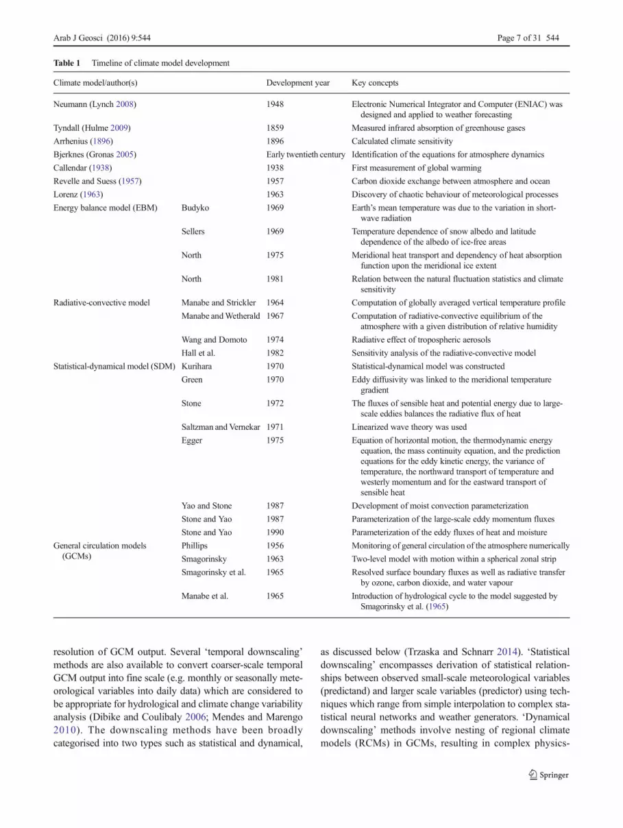
Temperature changes due to doubling of CO2 concentra-tion were analysed with the help of GCM (Manabe andWetherald 1975, 1980). The heat transport by large-scaleeddies was computed separately, and the results showed thatCO2 increase raises the temperature of the model troposphere,whilst it lowers that of the stratosphere (Manabe andWetherald 1975). Cloud prediction and extension of compu-tational domain up to the pole were performed byManabe andWetherald (1980). Stocker et al. (1992) developed a latitude-depth climate model by coupling three-basin ocean model forthe thermohaline circulation to the zonally averaged, one-layer energy balance model of the atmosphere. Stocker et al.(1992) did not consider separate water vapour budget for theatmosphere. Fanning andWeaver (1996) presented an integra-tion of energy-moisture balance model which allows the effectof latent heat transport (suggested earlier by Budyko 1969;Sellers 1969; and North 1975) with an OGCM (Pacanowskiet al. 1993;Weaver and Hughes 1996). The atmosphere modelconsists of a single vertically integrated layer, and the oceanmodel has 19 vertical levels with horizontal resolution of1.85° latitude by 3.75° longitude. Table 1 represents the time-line of the climate model development, highlights importantclimate model development years and contains the developedconcepts as well. Salient features of some coupled ocean–at-mosphere GCMs are mentioned in Table 2.
Downscaling: an approach to reduce the gapbetween GCMs’ ability and its utility in hydrologicalmodelling
GCMs are considered vital tools for the assessment of climatechange because they represent various earth systems includingthe atmosphere, oceans, land surface and sea ice (Fowler et al.2007). GCMs can further be coupled with hydrologicalmodels in order to assess the impact of climate change onhydrological regime (Larsen et al. 2014). However, the directapplication of GCMs coarse resolution outputs are often inad-equate to resolve significant regional scale features forassessing the effects of climate change on land surface pro-cesses, especially those pertaining to the hydrological cycle(Wilby andWigley 1997; Kidson and Thompson 1998;Wilbyet al. 1999; Xu 1999a). This problem can be addressedthrough the process of ‘downscaling’ that comprises determi-nation of local to regional scale information from large-scalemodelled or observed data and can be performed on bothspatial and temporal scales (Trzaska and Schnarr 2014).‘Spatial downscaling’ methods are used to derive climaticinformation at finer spatial resolution from coarser spatial
544 Page 6 of 31 Arab J Geosci (2016) 9:544
resolution of GCM output. Several ‘temporal downscaling’methods are also available to convert coarser-scale temporalGCM output into fine scale (e.g. monthly or seasonally mete-orological variables into daily data) which are considered tobe appropriate for hydrological and climate change variabilityanalysis (Dibike and Coulibaly 2006; Mendes and Marengo2010). The downscaling methods have been broadlycategorised into two types such as statistical and dynamical,
as discussed below (Trzaska and Schnarr 2014). ‘Statisticaldownscaling’ encompasses derivation of statistical relation-ships between observed small-scale meteorological variables(predictand) and larger scale variables (predictor) using tech-niques which range from simple interpolation to complex sta-tistical neural networks and weather generators. ‘Dynamicaldownscaling’ methods involve nesting of regional climatemodels (RCMs) in GCMs, resulting in complex physics-
Table 1 Timeline of climate model development
Climate model/author(s) Development year Key concepts
Neumann (Lynch 2008) 1948 Electronic Numerical Integrator and Computer (ENIAC) wasdesigned and applied to weather forecasting
Tyndall (Hulme 2009) 1859 Measured infrared absorption of greenhouse gases
Arrhenius (1896) 1896 Calculated climate sensitivity
Bjerknes (Gronas 2005) Early twentieth century Identification of the equations for atmosphere dynamics
Callendar (1938) 1938 First measurement of global warming
Revelle and Suess (1957) 1957 Carbon dioxide exchange between atmosphere and ocean
Lorenz (1963) 1963 Discovery of chaotic behaviour of meteorological processes
Energy balance model (EBM) Budyko 1969 Earth’s mean temperature was due to the variation in short-wave radiation
Sellers 1969 Temperature dependence of snow albedo and latitudedependence of the albedo of ice-free areas
North 1975 Meridional heat transport and dependency of heat absorptionfunction upon the meridional ice extent
North 1981 Relation between the natural fluctuation statistics and climatesensitivity
Radiative-convective model Manabe and Strickler 1964 Computation of globally averaged vertical temperature profile
Manabe andWetherald 1967 Computation of radiative-convective equilibrium of theatmosphere with a given distribution of relative humidity
Wang and Domoto 1974 Radiative effect of tropospheric aerosols
Hall et al. 1982 Sensitivity analysis of the radiative-convective model
Statistical-dynamical model (SDM) Kurihara 1970 Statistical-dynamical model was constructed
Green 1970 Eddy diffusivity was linked to the meridional temperaturegradient
Stone 1972 The fluxes of sensible heat and potential energy due to large-scale eddies balances the radiative flux of heat
Saltzman andVernekar 1971 Linearized wave theory was used
Egger 1975 Equation of horizontal motion, the thermodynamic energyequation, the mass continuity equation, and the predictionequations for the eddy kinetic energy, the variance oftemperature, the northward transport of temperature andwesterly momentum and for the eastward transport ofsensible heat
Yao and Stone 1987 Development of moist convection parameterization
Stone and Yao 1987 Parameterization of the large-scale eddy momentum fluxes
Stone and Yao 1990 Parameterization of the eddy fluxes of heat and moisture
General circulation models(GCMs)
Phillips 1956 Monitoring of general circulation of the atmosphere numerically
Smagorinsky 1963 Two-level model with motion within a spherical zonal strip
Smagorinsky et al. 1965 Resolved surface boundary fluxes as well as radiative transferby ozone, carbon dioxide, and water vapour
Manabe et al. 1965 Introduction of hydrological cycle to the model suggested bySmagorinsky et al. (1965)
Arab J Geosci (2016) 9:544 Page 7 of 31 544

based structure of the RCMs, and require high computationalcosts. Dynamical downscaling methods have gained impor-tance over statistical downscaling primarily due to lack of insitu data. Table 3 attempts to summarise some advantages anddisadvantages of both statistical and dynamical downscalingmethods.
In order to integrate the benefits of both the statistical anddynamical downscaling methods, some researchers have
recently combined both methods to develop a new ‘statistical-dynamical’ downscaling approach (Fuentes and Heimann2000; Vrac et al. 2012; Haas and Pinto 2012; Guyennon et al.2013; Trzaska and Schnarr 2014; Li et al. 2015). Statistical-dynamical downscaling method works by linking the globaland regional model simulations through statistics determinedfor large-scale weather types (Fuentes and Heimann 2000). Liet al. (2015) adopted statistical-dynamical downscaling
Table 2 Salient features of some coupled ocean–atmosphere GCMs
Climate model Resolution Key characteristics
ECHAM5/MPI-OMRoeckner et al. (2003)
• Pressure at the top = 10 hPa• Atmospheric model resolution (~1.9 × 1.9°) L31• Oceanic model resolution (1.5° × 1.5°) L40
• A flux-form semi-Lagrangian transport scheme• Separate prognostic equations for cloud liquid water
and cloud ice• New cloud microphysical scheme• Prognostic-statistical cloud cover parameterization• Increased spectral intervals in both the long-wave and
short-wave part of the spectrum
HadCM3Pope et al. (2000)
• Pressure at the top = 5 hPa• Atmospheric model resolution (2.5° × 3.75°) L19• Oceanic model resolution (1.25° × 1.25°) L20
• New radiation scheme• MOSES new land surface scheme• Convective momentum transport• Includes the radiative effects of aerosols and trace gases• Includes the effects of CO2 on evaporation at the land
surface
PRECIS (RCM)Jones et al. (2004)
• Horizontal resolution 50× 50 km • Seasonal and daily varying cycles of incoming solarradiation included
•Convective clouds and large-scale clouds are separatelytreated
• Run climate model for a range of emission scenarios
CGCM3.1 (www.ec.gc.ca/ccmac-cccma/default.asp?n=1299529F-1)
For T47 version• Atmospheric model resolution (3.75°) L31• Oceanic model resolution (~1.85°) L29For T63 version• Atmospheric model resolution (2.8°) L31• Oceanic model resolution (0.94° × 1.4°)
• Substantially updated atmospheric component• Provides better resolution of zonal currents in the
tropics• Reduced problems with converging meridians in the
Arctic
CSIRO Mk3.5Gordon et al. (2010)
• Pressure at the top = 4.5 hPa•Atmospheric component resolution (1.875° × 1.875°)
L18• Oceanic component resolution (1.875°× 0.9375°)
L31
• Upgraded ocean model to include spatially varyingeddy transfer coefficients and mixed layer scheme
• Improvement in oceanic behaviour in the high latitudeSouthern Ocean
• Reduced errors and climate drift
IPSL-CM5 (https://verc.enes.org/models/earthsystem-models/ipsl/ipslesm)
• Atmospheric model low resolution 1.9° × 3.75°(i.e. 9696 grid points) L39
• Atmospheric model mid resolution 1.25° × 1.25°(i.e. 143144 grid points) L39
• Oceanic model resolution 2° (meridional resolution0.5° near the equator)
It includes five component models• LMDz for atmospheric dynamics and physics• NEMO for ocean• ORCHIDEE for continental surfaces and vegetation• INCA for atmospheric chemistry• REPROBUS for stratospheric chemistry
MIROC4hSakamoto et al. (2012)
• Height of the model top = 40 km• Atmospheric component resolution (0.5625°)• Oceanic component resolution 0.28125° (zonal),
0.1875° (meridional)
• Errors in the surface air temperature and sea surfacetemperature are reduced
• Fine horizontal resolution in the atmosphere• Treatment of coastal upwelling motion in the ocean has
been improved•More vigorous ENSO events and related teleconnection
phenomena are reproduced
HadCM3Hadley Centre CoupledModel,MOSESMeteorological Office Surface Exchange Scheme, PRECIS Providing REgional Climates for ImpactsStudies, CGCM3.1 Coupled Global Climate Model, CSIRO-Mk3.5 Commonwealth Scientific and Industrial Research Organization Mark 3.5, IPSL-CM5 Institut Pierre-Simon Laplace-Climate Model, LMDz Laboratoire de Meteorologie Dynamique, NEMO Nucleus for European Modelling of theOcean, ORCHIDEE ORganising Carbon and Hydrology In Dynamic Ecosystems, INCA Interaction with Chemistry and Aerosols, REPROBUSREactive Processes Ruling the Ozone BUdget in the Stratosphere, MIROC4h Model for Interdisciplinary Research on Climate, L number of verticallevels
544 Page 8 of 31 Arab J Geosci (2016) 9:544

approach to reduce systematic biases in regional climate pro-jections by employing Community Climate System Model(CCSM) as a GCM and Weather Research and Forecasting(WRF) model coupled with the Community Land Model(CLM) as the RCM. They first implemented a statistical regres-sion technique and National Centers for EnvironmentalPrediction (NCEP) reanalysis data set to correct biases in theCCSM simulated variables. WRF simulations were then per-formed with the lateral boundary conditions being supplied bythe NCEP reanalysis, the original CCSM and the bias-correctedCCSM data. They observed that the bias-corrected CCSM dataresulted in a more realistic regional climate simulation.
Statistical downscaling
Asmentioned in the earlier section, the statistical downscalingmethods build statistical empirical relationships between theobserved small-scale meteorological variables (predictand)and larger scale variables (predictor) (Teutschbein 2013).Different approaches have been used by several researchersto classify the statistical downscaling methods based on thetechniques used (Wilby et al. 2004) and based on the selectedpredictor variables (Rummukainen 1997). Wilby et al. (2004)classified statistical downscaling methods into regressionmethods, weather pattern approaches and stochastic weathergenerators (WGs). On the other hand, Rummukainen (1997)classified statistical downscaling methods as downscalingwith surface variables, perfect prognosis (PP) and model out-put statistics (MOS) method. Maraun et al. (2010) reviewedand classified the statistical downscaling methods into threeclasses: WGs, PP andMOS. Table 4 summarises a few advan-tages and disadvantages of various statistical downscalingmethods. Some of the statistical downscaling methods basedon the techniques used, as described in the literature (Xu1999b; Wilby et al. 2004), are presented below.
1. Regression methods: Regression-based downscaling meth-od represents linear or nonlinear relationships betweenpredictand and predictors. Selection of the regression tech-nique for performing downscaling is based on the choice ofmathematical transfer function, statistical fitting procedureor predictor variable suite (Brooks and Legrand 2000).Some of the linear techniques include multiple regressions(Murphy 2000; Huth 2002, 2004), canonical correlationanalysis (Wigley et al. 1990; VonStorch et al. 1993; Huth2002, 2004; Chen and Chen 2003) and singular value de-composition (Benestad 2002; Widmann et al. 2003). Onthe other hand, nonlinear techniques employ the neuralnetworks self-organising maps (Hewitson and Crane1996; Wilby et al. 1998; Trigo and Palutikof 2001).
2. Weather pattern approaches: The weather pattern-based ap-proach involves grouping of local meteorological variablesin relation to different weather classification schemes(VonStorch et al. 1993; Wilby and Wigley 1997). Theseclassification schemes can be either subjectively or objec-tively derived; subjectivemethods primarily include BritishIsles Lamb Weather Types (Lamb 1972; Jones et al. 1993)and European Grosswetterlagen (Hess and Brezowsky1977), whilst objective methods include principal compo-nents (White et al. 1991), fuzzy rules (Bardossy et al. 1995)and correlation-based pattern recognition techniques (Lund1963). The major advantage of subjective methods is thatthe knowledge and experience of meteorologists can beused and is independent of the specific dataset used(Linderson 2001). Second advantage is that subjectivemethods are more straightforward for interpreting the phys-ical meaning of circulation patterns (Fan et al. 2015).Disadvantages of subjective methods are that the resultscannot be reproduced, and these methods can only be ap-plied for certain geographical areas (Bardossy et al. 2002).On the contrary, objective methods are dataset dependentand have a major advantage of allowing fast classification,
Table 3 Advantages and disadvantages of the statistical and dynamical downscaling methods
Statistical downscaling Dynamical downscaling
Advantages(Wilby et al. 2002;Trzaska and Schnarr2014)
• Station-scale information• Ensembles of climate scenarios permit uncertainty
analyses• Comparison across different case studies is possible
because the same method can be implemented acrossthe entire globe
• Cheap and technically less demanding than dynamicaldownscaling
• 20–50 km grid cell information• Ability to simulate smaller-scale atmospheric features, such
as orographic precipitation• Ability to respond in physically consistent ways to different
external forcings, such as land surface or atmosphericchemistry changes
• Better in terms of scientific understanding of the climatesystem
Disadvantages (Wilby et al.2002; Trzaska andSchnarr 2014)
• Climate change scenarios produced will be insensitiveto changes in land surface feedbacks
• Results are sensitive to the selection of domain size,location and predictor variables
• Selection of empirical transfer scheme affects the results• Model calibration requires high quality data
• High computational resources and expertise• Results are sensitive to the selection of domain size, location
and initial boundary conditions• Choice of cloud/convection scheme affects the results• Bias of driving GCM also affects the results
Arab J Geosci (2016) 9:544 Page 9 of 31 544

which is necessary especially for climate change scenarios(Bardossy et al. 2002).
3. Stochastic weather generators (WGs): WGs produce syn-thetic time series of weather data depending on the statis-tical characteristics of weather at that location (Wilks1992, 1999a; Semenov and Barrow 1997). Several WGsare available like Markov chain approach (Gelati et al.2010; Greene et al. 2011), the spell length approach(Racsko et al. 1991; Wilks 1999b) and mixture models(Carreau and Vrac 2011). Weather generators are data-intensive and generally require a long time series of dailydata (Soltani and Hoogenboom 2003). Weather genera-tion parameters are sensitive to missing data in the cali-bration set (Taulis and Milke 2005).
The other type categorisation for the statistical downscalingtechniques as proposed by Rummukainen (1997) based on thepredictor variable selection comprises the following:
1. Downscalingwith surface variables: This method developsa statistical relationship between the large-scale averages
of surface variables, which are developed from local timeseries and local-scale surface variables (Xu 1999b).
2. PP method: This method was used for the first time byKlein et al. (1959), and it basically involves the develop-ment of statistical relationships between large-scale freeatmospheric variables and local surface variables. Bothlarge-scale free atmospheric variables and local surfacevariables are observed quantities in the developmentalsample (Chen and Chen 2003).
3. The MOS method: MOS involves the development ofstatistical relationships between the large-scale free atmo-spheric variables, taken from GCM output and local sur-face variables (Glahn and Lowry 1972).
Dynamical downscaling
Dynamical downscaling method involves the nesting ofRCMs in GCMs; thus, this method is also called ‘nested’RCM approach (Teutschbein 2013) and nesting may be one-way or two-way (Harris and Durran 2010). If the RCM uses
Table 4 Advantages and disadvantages of different statistical downscaling methods
Statistical downscalingmethod
Advantages (Xu 1999b; Teutschbein 2013) Disadvantages (Xu 1999b; Teutschbein 2013) Examples (Teutschbein 2013)
Regression method(spatial)
• Straightforward to apply• Employs full range of available predictor
variables
• Inefficient for non-normally distributed data• Poor representation of observed variance• Inefficient for extreme events
• Multiple regressions• Canonical correlation
analysis• Singular value decomposition• Artificial neural networks
Weather pattern approach(spatial and temporal)
• Provides better understanding of theclimate sensitivity and variability
• Yields physically interpretable linkagesto surface climate
• It can be implemented to normally as wellas non-normally distributed data
• Additional work of weather classification isrequired
• Unable to predict the new values that lieoutside the range of the historical data
• Circulation-based schemes may beinsensitive to future climate forcing
• Fuzzy rules• Correlation-based pattern
recognition techniques• Principal components• Monte Carlo methods
Stochastic weathergenerator (spatial andtemporal)
• Provides sub-daily information• By interpolating the observed data it is
possible to obtain weather time series inregions of scarce data
• Comparatively ensembles of high-resolution climate scenarios may beproduced easily
• Arbitrary adjustment of parameters forfuture climate
• It is designed for the use of individuallocations independently and takes littleaccount of spatial correlation of climate
• Large amounts of observational datarequired to establish statisticalrelationships for the current climate
• Markov chain approach• The spell length approach• Mixture models• Stochastic methods
Perfect prognosis method • Strong relationships between large-scalefree atmospheric variables and localsurface variables because only currentobserved data is used
• Multiple predictors can be used whichresults in a better fit to the predictanddata
• Does not take into account the model bias• Cannot use important derived model
parameters as predictors, such as modelvertical velocity
The model output statisticsmethod (spatial andtemporal)
• Accounts for model variablespredictability by selecting those thatprovide more useful forecastinformation
• Takes into account the model bias• Good for longer range forecasts
• Relationship weakens with time due toincreasing model error variance
• Equations are model dependent
544 Page 10 of 31 Arab J Geosci (2016) 9:544
the GCM simulation output to define the initial and lateralboundary conditions, it is termed as ‘one-way nesting ap-proach’ (without feedback from RCM to GCM). On the otherhand, the ‘two-way nesting approach’ comprises a feedbackfrom RCM simulations back to the GCM. Two-way nestingapproach, which was originally developed by Anthes andWarner (1978), has been used by several researchers (Zhanget al. 1986; Warner et al. 1997; Debreu et al. 2012). However,the one-way nesting approach has also been used in manystudies (Colle et al. 2005; Deng and Stull 2005).
Teutschbein and Seibert (2010) reported that certain hydro-logical components such as surface and sub-surface runoff areincorporated by RCM simulations, but these simulations donot often agree with the streamflow observations. This is dueto the fact that RCM runoff schemes are not necessarily de-signed for accurate discharge calculation, but they do respondto general water balance tendencies (Van den Hurk et al.2005). Thus, RCM-simulated hydrological variables mightnot be directly useful for hydrological impact studies at thecatchment scale (Graham et al. 2007a). However, RCM-simulated variables such as temperature, precipitation andsnowpack are most commonly used as input to hydrologicalmodels (Graham et al. 2007a; Teutschbein and Seibert 2010).Several researchers (Varis et al. 2004; Graham et al. 2007a;Teutschbein and Seibert 2010) reported that even the RCM-simulated meteorological variables are often considerably bi-ased and their direct use in hydrological models may result ininappropriate simulations. To address this problem, severalRCMs can be used, as the application of several RCMs oftenleads to a wide spectrum of different simulation results, whichare often referred to as ‘ensemble simulations’ (Teutschbein2013). The same researcher has further reported that even themulti-model approaches (ensembles) often deviate from ob-servations, and therefore, further measures such as ‘bias cor-rection’ techniques are needed.
Climate model shortcomings, model errors and modelbiases
‘Model shortcomings’ originate because some climate modelsare unable to represent some parts of the climate system orunable to resolve certain processes related to the climate sys-tem, whichmay lead to ‘model errors’ (Teutschbein and Seibert2013). Furthermore, Deser et al. (2012) and Eden et al. (2012)described that ‘model errors’ may be caused by initial andboundary conditions, physical and numerical formulations,parameterizations or insufficient knowledge of externalfactors. Menard (2010) showed that model errors can appearas ‘systematic errors’ and ‘unsystematic (random) errors’.Allen et al. (2006) reported that systematic model errors mayeither arise from inadequately constrained parameters or frommodel structures that are incapable of describing the physicalprocesses of interest. For longer (centennial) timescales, these
systematic model errors are the major sources of uncertainty(Hawkins and Sutton 2011). On the other hand, unsystematic(random) model errors arise from the internal variability of theclimate models (internal variability occurs in the absence ofexternal forcing and includes processes intrinsic to the atmo-sphere, the ocean and the coupled ocean–atmosphere system)(Deser et al. 2012) and cause random variations in model sim-ulations (Teutschbein and Seibert 2013). For shorter (decadal)timescales, these unsystematic model errors are the majorsources of uncertainty (Hawkins and Sutton 2011).
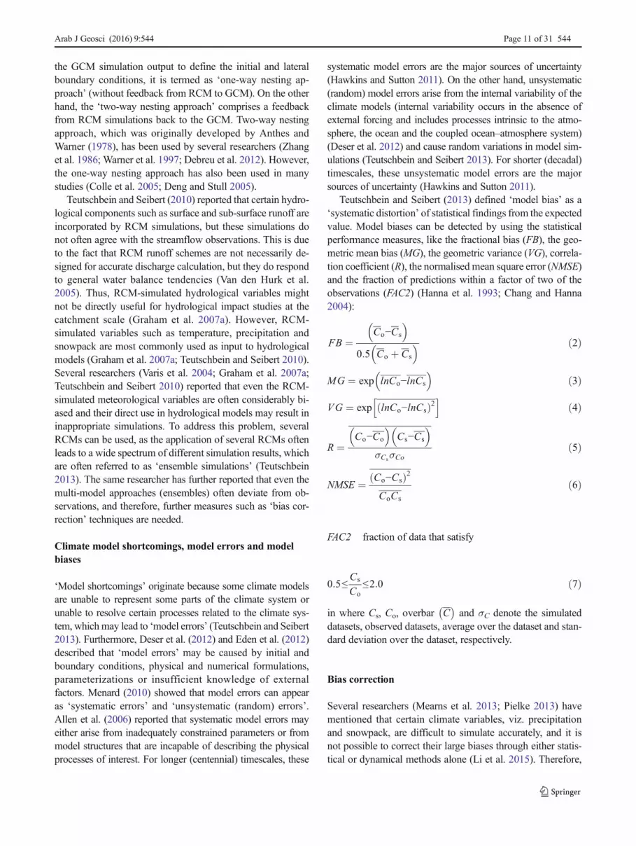
Teutschbein and Seibert (2013) defined ‘model bias’ as a‘systematic distortion’ of statistical findings from the expectedvalue. Model biases can be detected by using the statisticalperformance measures, like the fractional bias (FB), the geo-metric mean bias (MG), the geometric variance (VG), correla-tion coefficient (R), the normalised mean square error (NMSE)and the fraction of predictions within a factor of two of theobservations (FAC2) (Hanna et al. 1993; Chang and Hanna2004):
FB ¼Co−Cs
� �0:5 Co þ Cs
� � ð2Þ
MG ¼ exp lnCo−lnCs
� �ð3Þ
VG ¼ exp lnCo−lnCsð Þ2h i
ð4Þ
R ¼Co−Co
� �Cs−Cs
� �σCsσCo
ð5Þ
NMSE ¼ Co−Csð Þ2
CoCs
ð6Þ
FAC2 fraction of data that satisfy
0:5≤Cs
Co≤2:0 ð7Þ
in where Cs, Co, overbar C� �
and σC denote the simulateddatasets, observed datasets, average over the dataset and stan-dard deviation over the dataset, respectively.
Bias correction
Several researchers (Mearns et al. 2013; Pielke 2013) havementioned that certain climate variables, viz. precipitationand snowpack, are difficult to simulate accurately, and it isnot possible to correct their large biases through either statis-tical or dynamical methods alone (Li et al. 2015). Therefore,
Arab J Geosci (2016) 9:544 Page 11 of 31 544

there is a need of ‘bias correction’, which basically aims atcorrecting the systematic distortion/error in RCM-simulatedclimate variables by employing a transformation algorithm(Teutschbein and Seibert 2013). Ehret et al. (2012) outlinedthree main approaches to reduce the bias of climate models inorder to improve the efficiency of climate change impact stud-ies on hydrological regimes. These approaches can besummarised as follows:
1. Improving the GCMs and RCMs (it can be achieved byintegration of state-of-the-art hydrological models inGCMs/RCMs and improved process descriptions)
2. Including a multi-model ensemble approach: This may beachieved by using more than one GCMs, RCMs and/orhydrological models. Ensemble simulations have two ad-vantages: first, the spread of individual ensemble mem-bers represents more realistic observation and, second,ensemble median may tally with the observations better(Teutschbein and Seibert 2010)
3. Performing ‘bias correction’ (BC) techniques
BC techniques have been classified into delta-change ap-proach, linear scaling, local intensity scaling, variance scaling,power transformation and distribution transfer (detaileddescription of BC techniques can be found for example inTeutschbein and Seibert 2012). One major drawback of theBC method is the issue of ‘stationarity’, i.e. the correction algo-rithm and its parameterization for the current climate conditionsare assumed to remain the same in the future. In addition, theother disadvantages of BC method are mentioned as follows:
1. Physical causes of model errors, like temporal errors inmajor circulation systems or errors in the parameterizationof cloud and precipitation processes, are not considered(Teutschbein and Seibert 2012).
2. The links and feedbacks between the meteorologicalstates and fluxes (temperature, precipitation, humidity,evapotranspiration) are not taken into account (Ehretet al. 2012).
3. Conservation laws are not satisfied and cannot improvethe representation of fundamentally misrepresented phys-ical processes (Haerter et al. 2011).
4. In a complex modelling chain, the added value of biascorrection is questionable with other major sources ofuncertainty (Muerth et al. 2013).
5. Selection of the bias correction method forms an addition-al cause of uncertainty (Chen et al. 2011).
Ensemble approach
As discussed earlier, to reduce the bias of climate models, someresearchers apply an ensemble approach in order to improve the
efficiency of climate change impact studies on hydrologicalregimes. In ensemble approach, more than one GCM, RCMand/or hydrological models are used. Such approach was im-plemented in several research studies, for example to explorethe effects of warmer world scenarios on hydrological inputs toa Lake Malaren (Sweden), Moore et al. (2008) worked withtwo GCMs, i.e. the Max Planck Institute ECHAM4/OPYC3and the Hadley Centre HadAM3H for two IPCC emission sce-narios (A2, B2) and two RCMs, i.e. Rossby CentreAtmosphere–Ocean (RCAO) and Hadley Centre RegionalClimate Model (HadRM3p). Christensen and Lettenmaier(2007) used ensemble approach for the assessment of climatechange impacts on the hydrology of Colorado basin by using 11GCMs and two hydrological models, viz. Variable InfiltrationCapacity (VIC) and Colorado River Reservoir Model(CRMM). Diallo et al. (2012) used multi-model ensemble ap-proach over West Africa by analysing the performance of twoGCMs, namely ECHAM5 and HadCM3Q0, and four RCMs,i.e. International Centre for Theoretical Physics’ RegionalClimate Model (RegCM3), Max Planck Institute’s theRegional Model (REMO), Swedish Meteorological andHydrological Institute’s Rossby Centre Regional AtmosphericModel (RCA) and Met Office Hadley Centre (HadRM3p).Another complex experimental design was presented byGraham et al. (2007b). Based on two GCMs, HadAM3H andECHAM4/OPY3 for two IPCC emission scenarios (A2, B2),11 RCMs with resolutions of 50 km and two hydrologicalmodels, namely the Baltic basin Water Balance Model (HBV-Baltic) and the Water Flow and Balance Simulation Model(WASIM), the hydrological response to projected changes inthe climate was assessed by Graham et al. (2007b).
Intercomparison of downscaling methods
Several authors (Hewitson and Crane 1996; Xu 1999b; Yarnalet al. 2001; Fowler et al. 2007) reviewed downscaling methods.However, this section differs from previous reviews in that itfocuses on comparison and limitations of downscalingtechniques.
Chen et al. (2011) compared six downscaling methods, i.e.Canadian RCM (CRCM) with bias correction, CanadianRCM without bias correction, change factor (CF) method atboth Canadian GCM (CGCM) and CRCM scales, weathergenerator-based method at both CGCM and CRCM scales,statistical downscaling model (SDSM) at CGCM scale anddiscriminant analysis coupled with step-wise regression meth-od (DASR) at CGCM scale, to investigate the uncertainties inquantifying the impacts of climate change on the hydrology ofManicouagan 5 river basin located in central Quebec, Canadaover a reference period of 1970–1999. Overall, all of themethods, with the exception of CGCM-DASR, were goodbut CRCM data with bias correction and the SDSM proved
544 Page 12 of 31 Arab J Geosci (2016) 9:544
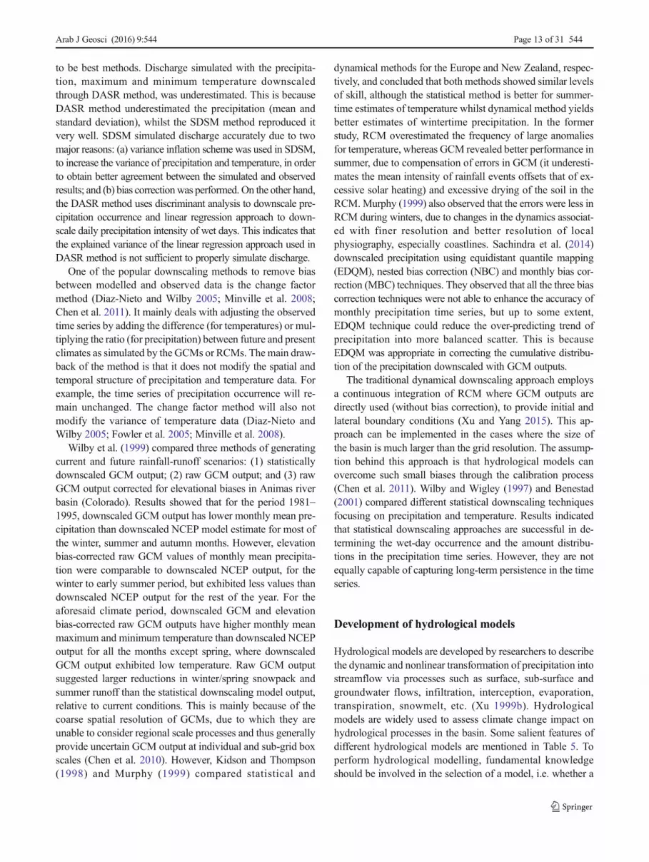
to be best methods. Discharge simulated with the precipita-tion, maximum and minimum temperature downscaledthrough DASR method, was underestimated. This is becauseDASR method underestimated the precipitation (mean andstandard deviation), whilst the SDSM method reproduced itvery well. SDSM simulated discharge accurately due to twomajor reasons: (a) variance inflation scheme was used in SDSM,to increase the variance of precipitation and temperature, in orderto obtain better agreement between the simulated and observedresults; and (b) bias correctionwas performed. On the other hand,the DASR method uses discriminant analysis to downscale pre-cipitation occurrence and linear regression approach to down-scale daily precipitation intensity of wet days. This indicates thatthe explained variance of the linear regression approach used inDASR method is not sufficient to properly simulate discharge.
One of the popular downscaling methods to remove biasbetween modelled and observed data is the change factormethod (Diaz-Nieto and Wilby 2005; Minville et al. 2008;Chen et al. 2011). It mainly deals with adjusting the observedtime series by adding the difference (for temperatures) or mul-tiplying the ratio (for precipitation) between future and presentclimates as simulated by the GCMs or RCMs. Themain draw-back of the method is that it does not modify the spatial andtemporal structure of precipitation and temperature data. Forexample, the time series of precipitation occurrence will re-main unchanged. The change factor method will also notmodify the variance of temperature data (Diaz-Nieto andWilby 2005; Fowler et al. 2005; Minville et al. 2008).
Wilby et al. (1999) compared three methods of generatingcurrent and future rainfall-runoff scenarios: (1) statisticallydownscaled GCM output; (2) raw GCM output; and (3) rawGCM output corrected for elevational biases in Animas riverbasin (Colorado). Results showed that for the period 1981–1995, downscaled GCM output has lower monthly mean pre-cipitation than downscaled NCEP model estimate for most ofthe winter, summer and autumn months. However, elevationbias-corrected raw GCM values of monthly mean precipita-tion were comparable to downscaled NCEP output, for thewinter to early summer period, but exhibited less values thandownscaled NCEP output for the rest of the year. For theaforesaid climate period, downscaled GCM and elevationbias-corrected raw GCM outputs have higher monthly meanmaximum and minimum temperature than downscaled NCEPoutput for all the months except spring, where downscaledGCM output exhibited low temperature. Raw GCM outputsuggested larger reductions in winter/spring snowpack andsummer runoff than the statistical downscaling model output,relative to current conditions. This is mainly because of thecoarse spatial resolution of GCMs, due to which they areunable to consider regional scale processes and thus generallyprovide uncertain GCM output at individual and sub-grid boxscales (Chen et al. 2010). However, Kidson and Thompson(1998) and Murphy (1999) compared statistical and
dynamical methods for the Europe and New Zealand, respec-tively, and concluded that both methods showed similar levelsof skill, although the statistical method is better for summer-time estimates of temperature whilst dynamical method yieldsbetter estimates of wintertime precipitation. In the formerstudy, RCM overestimated the frequency of large anomaliesfor temperature, whereas GCM revealed better performance insummer, due to compensation of errors in GCM (it underesti-mates the mean intensity of rainfall events offsets that of ex-cessive solar heating) and excessive drying of the soil in theRCM.Murphy (1999) also observed that the errors were less inRCM during winters, due to changes in the dynamics associat-ed with finer resolution and better resolution of localphysiography, especially coastlines. Sachindra et al. (2014)downscaled precipitation using equidistant quantile mapping(EDQM), nested bias correction (NBC) and monthly bias cor-rection (MBC) techniques. They observed that all the three biascorrection techniques were not able to enhance the accuracy ofmonthly precipitation time series, but up to some extent,EDQM technique could reduce the over-predicting trend ofprecipitation into more balanced scatter. This is becauseEDQM was appropriate in correcting the cumulative distribu-tion of the precipitation downscaled with GCM outputs.
The traditional dynamical downscaling approach employsa continuous integration of RCM where GCM outputs aredirectly used (without bias correction), to provide initial andlateral boundary conditions (Xu and Yang 2015). This ap-proach can be implemented in the cases where the size ofthe basin is much larger than the grid resolution. The assump-tion behind this approach is that hydrological models canovercome such small biases through the calibration process(Chen et al. 2011). Wilby and Wigley (1997) and Benestad(2001) compared different statistical downscaling techniquesfocusing on precipitation and temperature. Results indicatedthat statistical downscaling approaches are successful in de-termining the wet-day occurrence and the amount distribu-tions in the precipitation time series. However, they are notequally capable of capturing long-term persistence in the timeseries.
Development of hydrological models
Hydrological models are developed by researchers to describethe dynamic and nonlinear transformation of precipitation intostreamflow via processes such as surface, sub-surface andgroundwater flows, infiltration, interception, evaporation,transpiration, snowmelt, etc. (Xu 1999b). Hydrologicalmodels are widely used to assess climate change impact onhydrological processes in the basin. Some salient features ofdifferent hydrological models are mentioned in Table 5. Toperform hydrological modelling, fundamental knowledgeshould be involved in the selection of a model, i.e. whether a
Arab J Geosci (2016) 9:544 Page 13 of 31 544

Table 5 Salient features of some hydrological models
Hydrologicalmodel
Author(s) Spatial scale Application/output Key characteristics
DHSVM Wigmosta et al. (1994), Wigmosta andBurges (1997) and Wigmosta andLettenmaier (1999)
Continental,regional
Streamflow and snow waterequivalent
Distributed hydrological modelrepresents effects of vegetation andtopography on water fluxes
H08 Hanasaki andYamamoto (2010), Saitoand Hanasaki (2012)
River basin Quantitative estimate of the impactof reservoir operations on theterrestrial hydrological cycle;quantitative estimation of globalvirtual water trade
Simulate both natural water cycleand humanwater activities at dailybasis
VIC Liang et al. (1994) River basin Water and energy balance studies Sub-grid variability in land surfacevegetation classes; sub-gridvariability in the soil moisturestorage capacity; dynamiccoupling with GCMs or off-linesimulations
SWAT Rosenthal et al. (1995) Up to large riverbasin
Determination of climate and landmanagement impacts on waterquality and supply
Conceptual model and based oncontinuous time step; it simulateshydrology as a two-componentsystem, comprised of landhydrology and channel hydrology
Hydro-BEAM
Toshiharu (2005) 1–30 km Rainfall-runoff simulation Uses digital elevation models andGIS to simulate the runoff,provide ecosystem assessmentreports
WASMOD Schimming et al. (1995) Catchment Water balance studies, soil moistureindex, river flow, actualevapotranspiration modelling
Conceptual modelling system, basedon water balance plus nonlinearrelation between discharge andstorage; requires minimum5 years data for calibration
DWSM Borah et al. (2004) Watershed to sub-watershed
Total rainfall at each rain gauge,total watershed runoff, totaloutflow volume, flooding
Physically based, distributed anddeterministic modelling system
MIKEBASIN
Ireson et al. (2006) River basin Multi-purpose river network modelfor river basin management,simulation of natural inflows
Distributed and deterministic,conceptual modelling system; it isnot restricted to length ofsimulation period because it is acontinuous time-based model
MIKE 11 MIKE 11 user guide (www.hydroeurope.org/jahia/webdav/site/hydroeurope/shared/old/Teams-2011/team1/Manuals/MIKE11_UserManual.pdf), short introduction tutorial (www.tu-braunschweig.de/Medien-DB/geooekologie/mike-11-short-introduction-tutorial.pdf) and referencemanual (http://euroaquae.tu-cottbus.de/hydroweb/Platform/Notes/Mike11_Reference.pdf)
River basin Real-time flood forecasting,ecological and water qualityassessments in rivers
Deterministic mathematicalmodelling system; no limitationson the size of the model area ornumber of input elements to beincluded in the simulation
TOPKAPI Ciarapica and Todini (2002) Hill slope tocatchment
Generation of dischargehydrographs
Physically based distributed rainfall-runoff model; based on the idea ofcombining the kinematic approachwith the topography of the basin;characterised by three maincomponents: soil, overland flowand drainage network flow
UEB Tarboton (1994), Tarboton et al.(1995) and Tarboton and Luce(1996)
Point model(watershedgird)
Estimation of snow and glacier meltand outflow on grid distributedover a watershed
Uses physically based accounting ofradiative, sensible, latent andadvective heat exchanges tocalculate snowmelt
544 Page 14 of 31 Arab J Geosci (2016) 9:544

model should be ‘lumped’ or ‘distributed’ and ‘deterministic’or ‘stochastic’ (Beven 2001). The choice of a model dependson many factors and amongst them are the purpose of thestudy and the model availability (Ng and Marsalek 1992; Xu1999b). Monthly water balance models or rainfall-runoffmodels are useful for assessing water resource managementon a regional scale for identifying the consequences of chang-ing climatic variables on the hydrology (Alley 1984; Gleick1986; Arnell 1992). For surface flow estimation, conceptuallumped-parameter models are used (Chen et al. 2013; Tianet al. 2013), and for simulation of spatial patterns of hydro-logic response within a basin, process-based distributed-pa-rameter models are required (Beven 1989; Thomsen 1990).
Precipitation is the first major component of the terrestrialhydrological cycle, which after falling on the land surface joinsa stream or river and finally flows into the sea. The hydrologyof rainfall-dominated basins is more controlled by changes inprecipitation than temperature, whilst snowmelt-dominated ba-sins are highly sensitive to temperature changes (Praskieviczand Chang 2009). After precipitation, evapotranspiration (ET)is assumed to be the second largest component of terrestrialhydrological cycle (Mu et al. 2011). Theoretical approaches toevaporation from saturated surfaces were given by Penman(1948), and the direct response of stomata to the rate of tran-spiration rather than the humidity deficit was highlighted byMonteith (1995a, b). Penman-Monteith ET algorithm was de-veloped by several workers (Cleugh et al. 2007; Mu et al. 2011)for better performance in generating global ET data. Penman-Monteith method necessitates several climatic parametersthat are not always available mostly in the developingcountries; thus, simplified empirical methods were devel-oped using limited data to estimate potential ET (Zhaoet al. 2013). Simplified empirical methods include masstransfer, radiation, temperature and pan evaporation-basedmethods (Valipour 2015). Several researchers (Azhar andPerera 2011; Tabari et al. 2011; Djaman et al. 2015) re-ported that Penman-Monteith ET method is better thandifferent empirical ET methods, under various climaticconditions. A conceptual representation of the relationship
between different components of the hydrological cycle asmentioned by Freeze and Cherry (1979) is given in Fig. 3.
Mathematical hydrological modelling was initiated byDarcy (1856), who stated that water flow is proportional to agradient of hydraulic potential. Darcy’s linear relationship alsoholds good for unsaturated flow, but the constant of propor-tionality should be allowed to vary with soil moisture or cap-illary potential (Richards 1931). Horton (1933) gave a de-scription of runoff generation by highlighting the role of infil-tration in the hydrological cycle.
A basic rainfall-runoff model requires representations ofthe interaction between surface and sub-surface processes.A very simple approach unit hydrograph (UH) method, forrainfall-runoff modelling, was suggested by Sherman(1932). The UH of a catchment is defined as a direct runoffhydrograph resulting from a unit of excess rainfall gener-ated uniformly over the drainage area at a constant rate foran effective duration (Chow et al. 1988). Sherman’s ap-proach was based on the principle of superposition of ef-fects, in which it was assumed that the runoff hydrographof a particular rainfall can be superimposed with concur-rent runoff due to preceding rainfalls. However, Sherman’sUH was based on observed rainfall and runoff data; thus, itwas applicable only for gauged catchments. Hoffmeisterand Weisman (1977) reported that synthesis of a UH fromphysical basin characteristics is necessary for the extensionof the UH theory to un-gauged basins. In this context,several researchers (Snyder 1938; Gray 1961) relatedhydrograph characteristics (such as peak flow rate, basetime, etc.) to basin characteristics to generate synthetic unithydrographs (SUH) for un-gauged basins. In principle, aSUH retains all the features of an UH but does not requireobserved rainfall-runoff in its derivation. Different ap-proaches have been developed to generate SUH that havebeen categorised by Chow et al. (1988) into three majortypes, (1) those relating hydrograph characteristics to basincharacteristics (Snyder 1938; Gray 1961), (2) based ondimensionless UH (Soil Conservation Service 1957) and(3) based on models of watershed storage (Clark 1945).
Table 5 (continued)
Hydrologicalmodel
Author(s) Spatial scale Application/output Key characteristics
ArcEGMO Pfutzner et al. (1997) Sub-basin, basin,runoffcascades, riverreaches
Simulation of water balance, carbonand nitrogen budget
Conceptual; physically basedmultilayer; deterministic three-dimensional catchment model; itprovides 5 min to 1 day temporalscale modelling
DHSVM Distributed Hydrology Soil Vegetation Model, H08macro-scale hydrological model, VIC Variable Infiltration Capacity, SWAT Soil and WaterAssessment Tool,Hydro-BEAMHydrological River Basin Environment Assessment Model,GISGeographic Information System,WASMODWater andSnow balance MODelling system, DWSMDynamic Watershed Simulation Model, TOPKAPI TOPographic Kinematic APproximation and Integration,UEB Utah Energy Balance Snowmelt Model, ArcEGMO ArcInfo basiertes gegliedertes hydrologisches Modellsystem
Arab J Geosci (2016) 9:544 Page 15 of 31 544

On the other hand, Singh et al. (2014) classified SUH intofour main classes as follows:
1. Traditional or empirical SUH methods: These SUHmodels are based on different empirical equations andhave certain region-specific constants or coefficientsvarying over a wide range. Examples include Snyder(1938), Taylor and Schwarz (1952) and SoilConservation Service (SCS 1957).
(a) Snyder method: Snyder (1938) was first to estab-lish the empirical relationships, which relate thewatershed characteristics, such as area (Aw) insquare kilometer, length of main stream (L) in ki-lometer and the distance from the watershed outletto a point on the main stream nearest to the centreof the area of the watershed (Lc) in kilometer, tothe three basic parameters of the UH, i.e. the lag ortime to peak (tP) in hour, peak discharge rate (Qp)in cubic feet per second and base time (tb) in days.These relationships can be expressed as follows:
tP ¼ Ct LLcð Þ0:3 ð8Þ
Qp ¼ 640AwCp
tp
� �ð9Þ
tb ¼ 3þ 3tp24
� �ð10Þ
where Ct and Cp are non-dimensional constants and ingeneral vary from 1.8 to 2.2 and 0.56 to 0.69,
respectively. However, Eqs. 8 to 10 hold good forrainfall-excess duration (or unit duration tR)
tR ¼ tp.5:5 ð11Þ
(b) Taylor and Schwarz model: Taylor and Schwarz(1952) proposed a model for deriving the SUH,which specifically considers the average slope ofthe main channel of the watershed and watershedcharacteristics (i.e. Aw, L and Lc) which were similarto Snyder’s method. The average slope of the mainchannel is given as follows:
Sc ¼ NX N
i¼11.Si
� �0:5
264
3752
ð12Þ
where Sc is the average slope of the main channel, Si is theslope of the ith reach of the main channel and N is the totalnumber of reaches.
The empirical equations relating the UH characteristics towatershed characteristics are expressed as follows:
tP ¼ 0:6
Sc0:5
� e m1Dð Þ ð13Þ
Qp ¼382
LLcð Þ0:36" #
e m2Dð Þ ð14Þ
tb ¼ 5 tp þ tR2
h ið15Þ
where m1 =0.212(LLc)− 0.36, m2 =0.121Sc
0.142−0.05−m1, Dis rainfall duration and tP, L, Lc, tb and tR are same
Fig. 3 Conceptual representationof the relationship betweendifferent components of thehydrological cycle (source:Freeze and Cherry (1979))
544 Page 16 of 31 Arab J Geosci (2016) 9:544

as in Snyder’s method. However, the peak dischargerate (Qp) is expressed in cubic feet per second persquare mile.
(c) Soil Conservation Service method: The SCS (1957)method employs an average dimensionlesshydrograph developed from an analysis of a largenumber of natural unit hydrographs for watershedsof varying sizes located at different geographical lo-cations. SCS method represents the dimensionlessUH as a triangular UH, from which the runoff vol-ume (V) and peak discharge (qp) are computed asfollows:
V ¼ 0:5 qptb� �
¼ 0:5qp tp þ trc� � ð16Þ
trc ¼ 1:67 tp� � ð17Þ
qp ¼ 0:749V
tp
� �ð18Þ
where tb, tp and trc represent, respectively, base time, time topeak and time to recession expressed in hours, qp expressed inmillimeter per hour per millimeter and V in millimeter. Todetermine the complete shape of the SUH from the non-dimensional (q/qp versus t/tp) hydrograph, the time to peak iscomputed as follows:
tp ¼ tL þ tR.2 ð19Þ
where tL is lag time (hour) from the centroid of rainfall-excessto peak discharge (qp) in an hour and tR is the rainfall-excessduration (hour).
The lag time (tL) can be estimated from the watershed char-acteristics using the curve number (CN) procedure as follows:
tL ¼ L0:8 2540−22:86CNð Þ0:714; 104CN0:7Y 0:5 ð20Þ
where L is the length of the main stream or hydraulic length ofthe watershed (metre), CN is the curve number (50≤95) and Yis the average catchment slope (metre per metre).
Alternatively, Eq. 17 can be expressed as:
Qp ¼ 484Aw
tp
� �ð21Þ
whereQp is peak discharge in cubic feet per second of rainfall-excess and Aw is watershed area in square kilometer.2. Conceptual SUH methods: Conceptual models are based
on the continuity equation and linear storage dischargerelationship. Few examples include Clark (1945), Nash(1957) and Dooge (1959).
(a) Clark instantaneous unit hydrograph (IUH) model:Clark (1945) suggested that the UH for an area couldbe derived by routing its time–area concentrationcurve through an appropriate amount of reservoirstorage. In the routing procedure, an IUH is formed.IUH is defined as the hydrograph resulting from aninstantaneous rainfall of 1-inch. depth and durationequal to zero time. For the derivation of the IUH, theClark model uses two parameters, viz. time of con-centration (Tc) in hours, and storage coefficient (k) inhours of a single linear reservoir, in addition to thetime–area diagram. The governing equation of theClark IUH model can be expressed as follows:
ui ¼ C1Ai þ C2Ui−1 ð22Þwhere ui is the ith ordinate of the IUH, Ai the ith ordinateof the time–area diagram and C1 and C2 are Clark’srouting coefficients and can be computed by the followingexpressions:
C1 ¼ Δt
k þ 0:5Δtð Þ ð23Þ
C2 ¼ 1−C1 ð24Þwhere Δt is the computational interval in hour.
Finally, a UH of desired duration (D) can be derived byusing following equation:
Ui ¼ 1
N0:5ui−N þ ui−Nþ1 þ……þ ui−1 þ 0:5uið Þ ð25Þ
where Ui is the ith ordinate of the UH of D-hour duration andcomputational interval Δt hour, and N is the number of com-putational intervals in D-hour and is equal to D/Δt.
(b) Nash IUH model: The model proposed by Nash(1957) is based on the concept that IUH can be de-rived by routing the instantaneous inflow through acascade of linear reservoirs with equal storage coeffi-cient. The outflow from the first reservoir is consid-ered as inflow to the second reservoir and so on. Forderivation of IUH, the Nash model uses two parame-ters, viz. number of linear reservoirs (n), which isdimensionless and storage coefficient (K) in hours.The governing equation of the Nash IUH model isgiven as follows:
u tð Þ ¼ 1
KГ nð Þt
K
� �n−1e−
tK ð26Þ
where u(t) denotes IUH ordinates in hour−1, t is sampling timeinterval in hour and Г(n) is the well-known gamma function.
Arab J Geosci (2016) 9:544 Page 17 of 31 544

(c) Dooge IUH model: Dooge (1959) used the conceptof a linear channel and represented the basin by aseries of linear channels and linear reservoirs. Theoutflow from the linear channel was represented bya time–area diagram which, together with outflowfrom the preceding sub-area, serves as the inflow tothe linear reservoir. The expression developed for theIUH can be given as follows:
u tð Þ ¼ S
T
Z t0 ≤T
0
δ t−τð Þ∏
i τð Þi¼1 1þ KiDð Þ
0@
1Aω
τT
� �dτ
ð27Þwhere S is the input volume taken as unity, T is the totaltransmission time of the basin; i is the order of reservoirs equalto 1, 2, 3… counted downstream to the basin outlet; i(τ) is thefunction of τ representing an integer equal to the order numberof the sub-area;Ki is the storage coefficient of the ith reservoir;D is the differential operator (d/dt); δ(t− τ) is the Dirac-deltafunction, where t is the elapsed time; τ is the translation timebetween the elements in the sub-area and the outlet; andω(τ/T)is the ordinate of a dimensionless time–area diagram.3. Probabilistic or probability distribution function-based
SUHmethods: During last few decades, use of probabilitydistribution functions (pdfs) has received much attentionin developing SUH because of its similarity with UHproperties (Bhunya et al. 2007). Singh et al. (2014) report-ed two approaches, viz. non-parametric and parametricapproach, for the derivation of a UH from recorded floodhydrographs and simultaneous rainfall records. Non-parametric approach is based on a discretization tech-nique, i.e. determination of a model at a finite number ofdiscrete points. This includes the linear programming(Collins 1939), least squares method (Snyder 1955), ma-trix inversion (Eagleson et al. 1966), nonlinear program-ming (Mays and Taur 1982) and the transfer functionmethod (Yang and Han 2006). Parametric approach isthe one that fits some prescriptive functional curves witha limited number of parameters, and these parameters areestimated by means of optimization using an objectivefunction or through any suitable approach. Examples in-clude two-parameter gamma distribution (2PGD) (Nash1959 and Dooge 1959), three-parameter beta distribution(Mood et al. 1974), two-parameter Weibull distribution(Weibull 1939) and one-parameter chi-square distribution(Montgomery and Runger 1994).
4. Geomorphological instantaneous unit hydrograph(GIUH)-based SUH methods: The models pertaining tothis category couple the principles of hydrological sys-tems with the quantitative geomorphology of a basin.Examples include GIUH model, GIUH-based 2PGDNash model, width function-based GIUH model and
application of digital elevation models (DEMs) forGIUH-based hydrological modelling.
(a) GIUHmodel: Rodriguez-Iturbe andValdes (1979) intro-duced GIUH theory by relating IUH peak flow and timeto peakwith geomorphologic characteristics of the catch-ment and a dynamic velocity parameter. Equations werederived by Rodriguez-Iturbe and Valdes (1979) to ex-press peak flow and time to peak characteristics of theIUH as functions of Horton’s order ratios (Horton 1945).
(b) GIUH-based 2PGD Nash model: Rosso (1984)employed two-parameter gamma probability distri-bution function in order to develop SUH, in whichthe Nash model parameters were related to Horton’sorder ratios of a catchment on the basis of a geomor-phologic model of catchment response. The shapeparameter of the Nash model is found to be depen-dent on Horton’s numbers RA (area ratio), RS (bifur-cation ratio) and RL (length ratio) of a catchment;therefore, catchment geomorphology can provide asynthesis of the shape of the hydrologic response.The scale parameter of the Nash model depends onboth geomorphology and average streamflow veloc-ity along the stream network and the latter compo-nent renders it to be time dependent. As a result, thetime scale of the IUH could account for the variabil-ity of the hydrologic response for different stormsand throughout a storm.
(c) Width function-based GIUH model: One of the im-portant GIUH-based models is derived based on thegeomorphological width functionW(x), which is de-fined as the probability measure obtained by dividingthe number of links at a given distance x from theoutlet by the total number of links in the network,where x represents the distance to the outlet of the ithlink measured along the network and normalised bythe maximum path distance along the streams fromsource to outlet (Rinaldo and Rodriguez-Iturbe1996). The width functionW(x) helps in quantifyingthe influence of the network geometry on the runoffresponse of a basin (Kirkby 1976; Naden 1992).Further, the form of the width function also indicatesthe shape of the GIUH (Botter and Rinaldo 2003).
(d) Application of DEMs for GIUH-based hydrologicalmodelling: DEMs or digital terrain models (DTMs)have been used to extract different geomorphologi-cal parameters of drainage basins, including drainagenetworks, catchment divides, slope and aspect andupstream flow contributing areas (e.g. Jenson andDomingue 1988; Maidment et al. 1996).
Amongst the lumped models developed for esti-mating surface runoff from watersheds, SCS curvenumber method is a widely accepted method
544 Page 18 of 31 Arab J Geosci (2016) 9:544

because of its simplicity and limited number of pa-rameters required for runoff estimation (Liu and Li2008; Soulis and Valiantzas 2012; Candela et al.2014). The SCS curve number method was adoptedfor various regions, land uses and climate conditions(Elhakeem and Papanicolaou 2009; King andBalogh 2008) and became an integral part of hydro-logical models such as simulator for water resourcesin rural basins (SWRRB) (Williams et al. 1985),chemicals, runoff and erosion from agricultural man-agement systems (CREAMS) (Knisel 1980) and hy-drologic engineering centre-hydrologic modellingsystems (HEC-HMS) (USACE 2000).
Application of hydrological models to assess climatechange impact on the hydrological regime
There are a great number of studies, which have been carriedout to assess the possible effects of climate change on thehydrological regime. Figure 4 shows the integration of climateand hydrological models to assess the impact of climatechange on hydrological regime. The distinguishing characteris-tics of few recent studies are summarised in Table 6. At thebasin scale, major factors affecting climate change impacts onhydrological processes include latitude, topography, geologyand land use (Praskievicz and Chang 2009). One of the funda-mental characteristics determining a basin’s hydrological re-sponse to climate change is latitude. Several researchers (Jha2005; Thodsen 2007) reported increased runoff in humid mid-latitude basins for present and future period. Jha (2005) usedSoil and Water Assessment Tool (SWAT) and downscaled
GCMoutput to project impacts of climate change on hydrologyof Upper Mississippi river basin. The results indicated 51 %increase in surface runoff for future period (2040–2049).Thodsen (2007) used lumped hydrological model driven byan RCM, to simulate impacts of climate change on runoff infive major Danish rivers divided into 29 sub-catchments, andfound that mean annual runoff will increase by 12 % on aver-age, between a control period (1961–1990) and the future peri-od (2071–2100). Few researchers (Fujihara et al. 2008; Soodet al. 2013) reported a decrease in annual runoff in arid andsemi-arid basins. For example, Fujihara et al. (2008) modelledthe hydrological impacts of climate change in Seyhan riverbasin, Turkey, using the Hydrological River BasinEnvironmental Assessment Model (Hydro-BEAM) driven bytwo GCMs. The results indicated a decrease of 52–61 % inannual runoff for future (2070s) period. Sood et al. (2013) im-plemented SWAT driven by a downscaled GCM, to evaluateimpacts of climate change on hydrology of Volta river basin inWest Africa for 2021–2050 and 2071–2100, and marked anoverall decrease of up to 40 % in river flow.
Several efforts are made to improve the existingmodels through the use of advanced techniques such asfuzzy logic (Al-Zu’bi et al. 2010), artificial neural net-work (Akhtar et al. 2009) and linear prediction model(Zeng and Singh 1996). Several authors (Gleick 1986;Xu 1999a, b; Teutschbein and Seibert 2010) alsoreviewed modelling approaches to evaluate the impact ofclimate changes on hydrological regime, and Gleick(1986) concluded that monthly water balance models aremore useful in comparison to other methods in terms offlexibility, accuracy and ease of use. Few studies reportedthat the results of the climate change impact studies areless sensitive to the hydrological model as compared to
Fig. 4 Integration of climate andhydrological models to assessclimate change impact onhydrological regime
Arab J Geosci (2016) 9:544 Page 19 of 31 544

Tab
le6
The
distinguishing
characteristicsof
studiescarriedouttoassess
theim
pactof
clim
atechange
onhydrologicalregime
Author(s)
Study
basin
Clim
atemodel(s)
Baselineperiod
Future
clim
ate
change
projectio
nHydrologicalm
odel(s)
Results
Xuetal.(2014)
Jinhua
riverbasin
(China)
ECHAM5;
HadCM3;
PRECIS
1961–1990
2011–2040
DHSV
MECHAM5projectsdecrease
inrunoffduring
summer
(11.8%)andautumn(54.7%)
andslight
increase
during
spring
and
winter.HadCM3projectsdecreasesin
autumn(65%)andincreasesin
spring
(28.7%)andwinter(60%)
Masoodetal.(2014)
Ganges,Brahm
aputra
andMeghnariver
basins
(China,India,
Nepal,B
hutanand
Bangladesh)
MRI-AGCM3.2
1979–2003
2015–2039and
2075–2099
H08
Bytheendof
twenty-firstcentury,
temperature
risesby
3°C
.Anincrease
inmeanprecipitatio
nby
14,10.4and15.2
%andincrease
inmeanrunoffby
14,15and
18%
intheBrahm
aputra,G
angesand
Meghnabasin,respectiv
ely
Rajeetal.(2014)
Indian
riverbasins
BCCR-BCM
2.0;
CGCM3-T63;
CSIROMk3
1961–1990
2056–2065and
2083–2090
VIC
Increasing
trendforprojectedsummer
monsoon
surfacerunoff,
evapotranspiratio
nandsoilmoisturein
mostcentralIndian
riverbasins,w
hereas
adecrease
inrunoffandsoilmoistureis
projectedforsomeregionsin
southern
India
Sood
etal.(2013)
Voltariverbasin
(WestA
frica)
ECHAM;
COSM
O-CLM
1983–2012
2021–2050and
2071–2100
SWAT
Decreaseof
upto
40%
inriverflow
dueto
decreasing
rainfallandincreasing
temperature
Kankam-Yeboah
etal.(2013)
WhiteVoltaandPra
riverbasins
(Ghana)
ECHAM;C
SIRO
1983–2000(W
hite
Voltabasin)
and
1964–1991(Pra
basin)
2006–2035and
2036–2075
SWAT
Decreaseof
upto
50and46
%in
mean
annualstream
flow
during
2050sforthe
WhiteVoltaandPrabasin,respectiv
ely
Perazzolietal.
(2013)
Concordiariverbasin
(Brazil)
IPCCA2and
B2Scenario
1961–1990
2071–2100
SWAT
Com
parisonof
simulations
forA2andB2
scenarioswith
thebaselin
eshow
eda
decrease
instream
flow
of39.2and41.2
%,
respectiv
ely
Piniewskietal.
(2013)
Narew
riverbasin
(Poland)
IPSL-CM4;
MIROC3.2
1976–2000
2040–2069
WaterGAP;
SWAT
BetweenMay
andJune,M
IROC3.2suggests
anincrease
intemperatureby
3–3.5°C
and
smallchangein
precipitatio
nresulting
todecrease
inrunoffby
5.7mm
atZam
bski
usingSW
ATandnegligiblechange
using
WaterGAP.According
toMIROC3.2
increase
inprecipitatio
nandtemperatureis
53mm
and2.5–3.5°C
,respectively
544 Page 20 of 31 Arab J Geosci (2016) 9:544

Tab
le6
(contin
ued)
Author(s)
Study
basin
Clim
atemodel(s)
Baselineperiod
Future
clim
ate
change
projectio
nHydrologicalm
odel(s)
Results
during
August–Novem
ber.Thisresults
inincrease
inrunoffby
8.4and3mm
using
SWATandWaterGAP,respectiv
ely.
Shresthaetal.
(2012)
Red
andAssiniboine
basins
intheLake
Winnipeg
watershed
(Canada)
CRCM;R
CM3;
HRM3
1980–2000
2042–2062
SWAT
Resultsrevealed
higher
totalrunoff,earlier
snow
meltand
dischargepeaks
Maureretal.(2009)
Rio
Lem
pabasin
(CentralAmerica)
16GCMs
1961–1990
2040–2069and
2070–2099
VIC
Medianreservoirinflow
decreasesby
13%
(B1)
and24
%(A
2)during
2070–2099,
mediantemperature
increasesby
1.9°C
(B1)
and3.4°C
(A2),respectively,and
medianprecipitatio
ndecreasesby
5.0%
(B1)
and10.4
%(A
2)
Fujiharaetal.(2008)
Seyhanriverbasin(Turkey)
MRI-CGCM2;
CCSR
/NIES/FRCGC-M
IROC
1990s
2070s
Hydro-BEAM
Decreasein
annualrunoffof
52–61%,
increase
inaverageannualtemperature
change
was
2°C
inMRIand2.7°C
inCCSR
,and
theaverageannual
precipitatio
ndecreasedby
159mm
inMRIand161mm
inCCSR
Islam
etal.(2014)
Murray-Hotham
Catchment
(Western
Australia)
11GCMs
1961–2000
2046–2065and
2081–2100
LUCICAT
Reductio
nby
2.3%
inthemeanannual
rainfallaveraged
overthecatchm
entduring
1981–2000andrunoffreductionby
14%
Tramblay
etal.
(2013)
Makhazine
dam
basin
(North
Morocco)
High-resolutio
nRCM
(ALADIN
-Clim
ate)
1984–2010
2041–2062
GR4J
Forthefuturescenarios(2041–2062),surface
runoffwould
decrease
by−3
0to
−57%,
whenforthesameperiod
theprojectio
nsforprecipitatio
nranges
between−1
5and
−19%
andfortemperature
between+1.3
and+1.9°C
Joigneauxetal.
(2011)
Vald’Orleans
(France)
ARPE
GEScenario;
GISS-
AOM;
GISS-ER;M
IROC3.2-
(medres);
MIU
B-ECHO-G
1966–2009
2075–2099
GARDENIA
(catchmentm
odel)
During2075–2099,decrease
inback-flooding
eventscanbe
expected.D
ueto
this,the
potentialriskforgroundw
aterquality
inthe
catchm
entareawill
begreatly
reduced
Steele-D
unne
etal.
(2008)
Ninecatchm
ents(M
oy,S
uck,
Brosna,Boyne,B
arrow,
Suir,Feale,Blackwater,
Bandon)
(Ireland)
ECHAM5-OM1;
RCA3
1961–2000
2012–2060
HBV-Light
conceptual
rainfall-runoffmodel
Anam
plificationof
theseasonalcycleacross
thecountry,driven
byincreasedwinter
precipitatio
n,decreasedsummer
precipitatio
nandincreasedtemperaturehas
been
suggested
Arab J Geosci (2016) 9:544 Page 21 of 31 544

Tab
le6
(contin
ued)
Author(s)
Study
basin
Clim
atemodel(s)
Baselineperiod
Future
clim
ate
change
projectio
nHydrologicalm
odel(s)
Results
Khoiand
Hang
(2015)
The
Srepokwatershed,a
sub-basinof
theMekong
riverbasin(Central
Highlands
ofVietnam
)
HadCM3;
CCCMA
CGCM3.1;
CSIRO
Mk3.0;ISP
LCM4;
MPI
ECHAM5;
NCARCCSM
3.0;
UKMOHadGEM1;
SRESem
ission
scenarios
(A1B
,A2,
B1andB2)
1970–2000
2006–2100
SWAT
HadCM3suggestsalin
eardecrease
inthe
meanannualstream
flow
rangingfrom
2to
9.8%.P
rojected
annualstream
flow
differencesbetweenSR
ESem
ission
scenariosusingHadCM3weresm
all(−3
.8to−3
.3%).With
a2°C
riseinglobalmean
temperature,the
projectedchangesin
river
dischargevary
from
−6to
16.1
%
Shrestha
(2014)
25River
basins
(Thailand)
PRECIS
RCM
1971–2000
2011–2100
HEC-H
MS
Anincrease
inprecipitatio
nfrom
21.4to
37.8
%(A
2scenario)and15.4to
30.6
%(B2scenario)isexpected
intheMae
Kok,
BangPakong,M
aeKhong
andSouthern
basinHRUsby
2080s.The
natio
nallevel
water
availabilityvaries
from
−5.5
%in
2020sto
+13
%in
2090sand+1%
in2010sto
+29
%in
2080s
Peleg
etal.(2015)
The
upperDalya;
andupperTaninim
catchm
ents(north-
western
Israel)
CMIP5
1996–2005
2046–2055
SCA-SMA
The
meanannualrainfallisprojectedto
bedecreasedby
15and18
%fortheRCP4
.5andRCP8
.5em
ission
scenarios,
respectiv
ely.Reductio
ninthemeanannual
stream
flow
volumes
isprojectedto
be45
and47
%.T
hestream
flow
season
isprojectedto
beshorterby
22and26–28%
fortheRCP4
.5andRCP8
.5,scenarios,
respectiv
ely
Bocchiolaetal.
(2011)
HKHRegion
(northernPakistan)
NCAR-CCSM
31985–1997
2050–2059
DHM
Anincrease
oftemperature
of+1.9°C
onaverage,with
respecttothecontrolp
eriod
2000–2009.Increm
entinprecipitatio
n,+20
%or
so.Increasein
averageicemelt
asaconsequenceof
increasedtemperature
Hatterm
annetal.
(2014)
The
northern
German
lowlands,
thecentralG
erman
upland,
thesouthw
estern
Rhine
Valley,theAlpineforeland
andtheGerman
Alps(G
ermany)
ECHAM5;
CCLM;R
EMO
1961–2000
2100
sSW
IMIn
thefuture
underthespecificscenario
conditions,aconsiderableincrease
inflood
relatedlosses
canbe
expected
inGermany
544 Page 22 of 31 Arab J Geosci (2016) 9:544

Tab
le6
(contin
ued)
Author(s)
Study
basin
Clim
atemodel(s)
Baselineperiod
Future
clim
ate
change
projectio
nHydrologicalm
odel(s)
Results
Hontietal.(2014)
The
MonchaltorferAaandthe
Gurbe
catchm
ent,(SwissPlateau)
10GCM–R
CM
1981–2010
2035–2064
CRRM
Expectedclim
aticim
pacton
flow
quantiles
was
smallcom
paredto
predictio
nuncertainty.Resultssuggestthatfuture
flow
conditionsmay
developin
quite
differentd
irectio
nsin
thefuture,
irrespectiv
eof
uncertaintyassessment
methodandflow
quantile
HadCM3HadleyCentreCoupled
Model,version
3,PRECIS
ProvidingREgionalClim
ates
forIm
pactsStudies,D
HSV
MDistributed
Hydrology
SoilV
egetationModel,M
RI-AGCM3.2Meteorological
ResearchInstitu
te-A
tmosphericGeneralCirculatio
nModel,version
3.2,H08
macro-scalehydrologicalmodel,B
CCR-BCM
2.0BjerknesCentreforClim
ateResearch-BergenClim
ateModel,version
2.0,
CGCM3Coupled
GlobalC
limateModel,version
3,CSIROMk3
Com
monwealth
ScientificandIndustrialResearchOrganizationMark3,VIC
VariableInfiltrationCapacity,C
OSM
O-CLM
Consortiumfor
Small-scaleModellin
g-Clim
ateLim
ited-area
Modellin
g,SW
ATSoilandWater
Assessm
entTo
ol,CSIRO
Com
monwealth
ScientificandIndustrial
ResearchOrganization,
IPSL
CM4L’Institu
tPierre-
Simon
Laplace
Coupled
Model,version
4,MIROC3.2ModelforInterdisciplin
aryResearchon
Clim
ate,version3.2,WaterGAPWater:A
GlobalA
nalysisandPrognosis,SW
ATSoiland
WaterAssessm
ent
Tool,CRCM
CanadianRCM,HRM3HadleyRegionalModel
3,MRI-CGCM2MeteorologicalResearchInstitu
teCoupled
Atm
osphere–Ocean
General
Circulatio
nModel,version2,
Hydro-BEAM
HydrologicalR
iverBasinEnvironmentA
ssessm
entM
odel,LUCICATtheLandUse
ChangeIncorporated
CATchm
ent,ALADIN
AireLim
iteeAdaptationdynamique
DeveloppementInterNational,GR4J
Genie
Rural
a4parametresJournalier,ARPEGEActionde
Recherche
PetiteEchelle
GrandeEchelle,GISS-AOM
Goddard
Institu
teforSp
aceStudies-Atm
ospheric
Ocean
Model,GISS-ERGoddard
Institu
teforSpace
Studies-M
odelE,coupledwith
theRusselloceanmodel,MIROC3.2ModelforInterdisciplinaryResearchon
Clim
ate,version3.2,
MIU
B-ECHO-G
MeteorologicalInstitu
teof
the
University
ofBonn,ECHO-G
Model(ECHAM4andtheGlobalH
amburgOcean
Prim
itive
Equation),G
ARDENIA
GlobalA
ReservoirspourlasimulationdesDEbitsetdesNIveaux
Aquiferes,E
CHAM5-
OM1EuropeanCentreHam
burg
Model,v
ersion
5-Ocean
Model,v
ersion
1,RCA3RossbyCentreRegionalAtm
osphericClim
ateModel,v
ersion
3,HBVHydrologiskaByransVattenbalansavdelning,
CCCMACGCM3.1CanadianCentreforC
limateModellin
gandAnalysisCoupled
GlobalC
limateModel,version
3.1,CSIROMk3.0Com
monwealth
ScientificandIndustrialResearchOrganizationMark
3.0,
IPSL
CM4L’Institu
tPierre-Simon
Laplace
Coupled
Model,version4,
MPIECHAM5Max
PlanckInstitu
teEuropeanCentreHam
burg
Model,version5,
NCARCCSM
3.0NationalCenterfor
Atm
osphericResearchCom
munity
Clim
ateSystem
Model,v
ersion
3,UKMO
HadGEM1UnitedKingdom
MetOfficeHadleyCentreGlobalEnvironmentModel,v
ersion
1,SR
ESSpecialReporton
EmissionsScenarios,SW
ATSoilandWater
Assessm
entTo
ol,PRECIS
ProvidingREgional
Clim
ates
forIm
pactsStudies,HEC-H
MSHydrologicEngineering
Center-HydrologicModellin
gSy
stem
,CMIP5Coupled
ModelIntercom
parisonProjectP
hase
5,SC
A-SMAtheSacramento
SoilM
oistureAccountingModel,H
KHHindu
Kush,Karakoram
andHim
alaya,NCAR-CCSM
3NationalC
enterfor
Atm
osphericResearchCom
munity
Clim
ateSy
stem
Model,version
3,DHM
Distributed
HydrologicalM
odel,C
CLM
COSMO-Clim
ateLim
ited-area
Modellin
g,REMOREgionalModel,SWIM
Soiland
Water
Integrated
Model,C
RRM
ConceptualR
ainfall-RunoffModel
Arab J Geosci (2016) 9:544 Page 23 of 31 544

the climate change scenario (Graham et al. 2007b; Kayet al. 2009). In other words, different hydrological modelsif allowed to run with the same climatic inputs tend toproduce similar results, whereas same hydrological modelrun under different GCM simulations may give differentresults.
Conclusions
This article reviews hierarchy and development of climatemodels from the early times, importance and inter-comparison of various downscaling techniques and develop-ment of hydrological models. Also recent research develop-ments regarding the evaluation of climate change impact onthe hydrological regime have been discussed. The article alsoprovides some suggestions to improve the modelling ap-proaches involved in evaluation of climate change impact onhydrological regime.
One of the major challenging factors in the climate model-ling is the complexity of the climate system and the manner inwhich several processes interact with each other. Each climatemodel has a slightly different way of describing oceans, atmo-sphere, land and continental ice and the fluxes amongst eachother. Therefore, different climate models provide differentclimate projections even for the same region over a particulartime period.
Hydrological modelling is a significant tool for solvingseveral issues related to hydrology and for analysing thesensitivity of hydrological regime to climate variabilityespecially in developing countries. One of the possibleways to achieve this is the integration of climate and hy-drological models. However, GCMs were basically de-signed to predict the general circulation patterns of theatmosphere but not for climate change impact studies onhydrological regime. Their outputs are not able to resolvesignificant regional scale features for assessing the effectsof climate change on land surface processes, especiallyhydrology. In this regard, significant downscaling tech-niques, i.e. statistical and dynamical downscalingmethods, are developed to realistically simulate regionalclimate features up to some extent. However, certain cli-mate variables, such as precipitation and snowpack, areparticularly difficult to simulate accurately, and it is diffi-cult to correct their large biases through either dynamicalor statistical methods alone. Therefore, there is a dire needto implement bias correction procedures to ensure thatGCM and RCM simulation outputs perform satisfactorilyfor hydrological impact studies. Climate models have notonly proven to be valuable tools for the projection offuture climate change but also for the assessment of cli-mate change impact on the hydrological regime.
Suggestions
Based on this review, following points are suggested to im-prove the effectiveness of modelling approach for the assess-ment of climate change impact on hydrological regime:
1. Development in climate modelling by improving the abil-ity to transform the existing knowledge into accuratemathematical equations. Improved understanding of theclimate system can significantly reduce the inaccuraterepresentations of the interaction of several processes inmodelling.
2. Dynamical downscaling inaccuracy can be reducedthrough improvements in the representation of physicalprocesses at higher resolution. On the other hand, accura-cy of statistical downscaling would depend on the tempo-ral availability of local predictand so that they can beeffectively used for screening of suitable predictor vari-ables. If the local predictand is subject to changes notpresent in predictors, multiple variable types as predictorscan be used to account for each changing variable thataffects the local climate.
3. High relief in terrains could cause large-scale heterogene-ity in the atmospheric variables at different altitudes.Therefore, in such terrains screening of predictors at ap-propriate pressure levels could improve the accuracy ofdownscaling, modelling and prediction of climaticvariables.
4. To reduce the biases between the observed and simulatedclimate variables, ensemble simulations can be construct-ed using different GCMs with different climate sensitivityunder different greenhouse gas emission scenariosstarting from different initial conditions.
5. Improved knowledge of the relationship amongst differ-ent climate variables and use of advanced statistical tech-niques (in conjunction with soft computing techniques)for observing significant changes in the frequency andintensity of extreme events.
6. There is a dire need to carry out more comprehensiveresearches with better coordinated inputs for achievingopen access to model setups and hydro-meteorologicaldata.
Acknowledgments The authors are highly grateful to the editor andanonymous reviewers for their insightful and valuable comments, whichenabled us to improve the manuscript to the present state.
References
Akhtar MK, Corzo GA, van Andel SJ, Jonoski A (2009) River flowforecasting with artificial neural networks using satellite observedprecipitation pre-processed with flow length and travel time
544 Page 24 of 31 Arab J Geosci (2016) 9:544

information: case study of the Ganges river basin. Hydrol Earth SystSci 13:1607–1618
AlexanderMA, Scott JD,Mahoney K, Barsugli J (2013) Greenhouse gas-induced changes in summer precipitation over Colorado inNARCCAP regional climate models. J Clim 26:8690–8697
Allen M, Frame D, Kettleborough J, Stainforth D (2006) Model error inweather and climate forecasting. In: Predictability of weather andclimate. Cambridge University Press, pp 391–427
Alley WM (1984) On the treatment of evapotranspiration, soil moistureaccounting, and aquifer recharge in monthly water balance models.Water Resour Res 20:1137–1149
Al-Zu’bi Y, Sheta A, Al-Zu’bi J (2010) Nile river flow forecasting basedon Takagi-Sugeno fuzzy model. J Appl Sci 10:284–290
Anderegg WRL, Prall JW, Harold J, Schneider SH (2010) Expert credi-bility in climate change. Proc Natl Acad Sci 107:12107–12109
Andrews T, Gregory JM,WebbMJ, Taylor KE (2012) Forcing, feedbacksand climate sensitivity in CMIP5 coupled atmosphere–ocean cli-mate models. Geophys Res Lett 39:L09712
Angstrom A (1926) Energiezufuhr und temperatur auf verschiedenenBreitengraden. Gerlands Beitr Geophysik 15:1–13
Annan JD, Hargreaves JC (2006) Using multiple observationally-basedconstraints to estimate climate sensitivity. Geophys Res Lett 33:L06704
Anthes RA, Warner TT (1978) Development of hydrodynamic modelssuitable for air pollution and other mesometerological studies. MonWeather Rev 106:1045–1078
Armour KC, Bitz CM, Roe GH (2013) Time-varying climate sensitivityfrom regional feedbacks. J Clim 26:4518–4534
Arnell NW (1992) Factors controlling the effects of climate change onriver flow regimes in a humid temperate environment. J Hydrol 132:321–342
Arrhenius S (1896) On the influence of carbonic acid in the air upon thetemperature of the ground. Philos Mag 41:237–276
Azhar AH, Perera BJC (2011) Evaluation of reference evapotranspirationestimation methods under southeast Australian conditions. J IrrigDrain Eng 137:268–279
Bardossy A, Duckstein L, Bogardi I (1995) Fuzzy rule-based classificationof atmospheric circulation patterns. Int J Climatol 15:1087–1097
Bardossy A, Stehlik J, Caspary HJ (2002) Automated objective classifi-cation of daily circulation patterns for precipitation and temperaturedownscaling based on optimized fuzzy rules. Clim Res 23:11–22
Benestad RE (2001) A comparison between two empirical downscalingstrategies. Int J Climatol 21:1645–1668
Benestad RE (2002) Empirically downscaled multimodel ensemble temper-ature and precipitation scenarios for Norway. J Clim 21:3008–3027
Bernard L, Semmler W (eds) (2015) The oxford handbook of the macro-economics of global warming. Oxford University Press, New York
Beven KJ (1989) Changing ideas in hydrology: the case of physicallybased models. J Hydrol 105:157–172
Beven KJ (2001) Rainfall-runoff modelling: the primer. Wiley,Chichester
Bhunya PK, Berndtsson R, Ojha CSP, Mishra SK (2007) Suitability ofgamma, chi-square, Weibull, and beta distributions as synthetic unithydrographs. J Hydrol 334:28–38
Bocchiola D, Diolaiuti G, Soncini A, Mihalcea C, D’Agata C, Mayer C,Lambrecht A, Rosso R, Smiraglia C (2011) Prediction of future hydro-logical regimes in poorly gauged high altitude basins: the case study ofthe upper Indus, Pakistan. Hydrol Earth Syst Sci 15:2059–2075
Borah DK, Bera M, Xia R (2004) Storm event flow and sediment simu-lations in agricultural watersheds using DWSM. Trans ASAE 47:1539–1559
Botter G, Rinaldo A (2003) Scale effect on geomorphologic and kine-matic dispersion. Water Resour Res 39:1286
Brooks N, Legrand M (2000) Dust variability over Northern Africa andrainfall in the Sahel. In: Linking climate change to land surface
change. Kluwer Academic Publishers, Dordrecht/Boston/London,pp 1–25
Bryan K (1969) Climate and the ocean circulation III. The ocean model.Mon Weather Rev 97:806–827
Bryan K, Cox MD (1967) A numerical investigation of the oceanic gen-eral circulation. Tellus 19:54–80
Bryan K, Cox MD (1968a) A nonlinear model of an ocean driven bywind and differential heating: part I. Description of the three-dimensional velocity and density fields. J Atmos Sci 25:945–967
Bryan K, Cox MD (1968b) A nonlinear model of an ocean driven bywind and differential heating: part II. An analysis of the heat, vor-ticity and energy balance. J Atmos Sci 25:968–978
Budyko MI (1969) The effect of solar radiation variations on the climateof the earth. Tellus 21:611–619
Callendar GS (1938) The artificial production of carbon dioxide and itsinfluence on temperature. Q J R Meteorol Soc 64:223–240
Candela A, Brigandi G, Aronica GT (2014) Estimation of synthetic flooddesign hydrographs using a distributed rainfall-runoff modelcoupled with a copula-based single storm rainfall generator. NatHazards Earth Syst Sci 14:1819–1833
Carreau J, Vrac M (2011) Stochastic downscaling of precipitation withneural network conditional mixture models. Water Resour Res 47:W10502
Chang JC, Hanna SR (2004) Air quality model performance evaluation.Meteorog Atmos Phys 87:167–196
Chen DL, Chen YM (2003) Association between winter temperature inChina and upper air circulation over East Asia revealed by canonicalcorrelation analysis. Glob Planet Chang 37:315–325
Chen H, Guo J, Xiong W, Shenglian G, Xu CY (2010) DownscalingGCMs using the smooth support vector machine method to predictdaily precipitation in the Hanjiang basin. Adv Atmos Sci 27:274–284
Chen J, Brissette FP, Leconte R (2011) Uncertainty of downscaling meth-od in quantifying the impact of climate change on hydrology. JHydrol 401:190–202
Chen J, Brissett FP, Chaumont D, Braun M (2013) Performance anduncertainty evaluation of empirical downscaling methods in quanti-fying the climate change impacts on hydrology over two NorthAmerican river basins. J Hydrol 479:200–214
Chow VT, Maidment DR, Mays LW (1988) Applied hydrology.McGraw-Hill, New York
Christensen NS, Lettenmaier DP (2007) A multimodel ensemble ap-proach to assessment of climate change impacts on the hydrologyand water resources of the Colorado river basin. Hydrol Earth SystSci 11:1417–1434
Ciarapica L, Todini E (2002) TOPKAPI: a model for the representation ofthe rainfall-runoff process at different scales. Hydrol Process 16:207–229
Clark CO (1945) Storage and the unit hydrograph. Trans Am Soc CivEng 110:1419–1446
Cleugh HA, Leuning R, Mu Q, Running SW (2007) Regional evapora-tion estimates from flux tower and MODIS satellite data. RemoteSens Environ 106:285–304
Colle BA,Wolfe JB, SteenburghWJ, Kingsmill DE, Cox JAW, Shafer JC(2005) High-resolution simulations and microphysical validation ofan orographic precipitation event over the Wasatch Mountains dur-ing IPEX IOP3. Mon Weather Rev 133:2947–2971
Collins WT (1939) Runoff distribution graphs from precipitation occur-ring in more than one time unit. Civ Eng 9:559–561
Collins M, Knutti R, Arblaster J, Dufresne JL, Fichefet T, FriedlingsteinP, GaoX, Gutowski JrWJ, Johns T, Krinner G, ShongweM, TebaldiC, Weaver AJ, Wehner M (2013) Long-term climate change: pro-jections, commitments and irreversibility. In: Climate change 2013:the physical science basis. Contribution of Working Group I to theFifth Assessment Report of the Intergovernmental Panel on ClimateChange. Cambridge University Press, Cambridge, pp 1029–1136
Arab J Geosci (2016) 9:544 Page 25 of 31 544

Corney S, Grose M, Bennett JC, White C, Katzfey J, McGregor J, HolzG, Bindoff NL (2013) Performance of downscaled regional climatesimulations using a variable-resolution regional climate model:Tasmania as a test case. J Geophys Res Atmos 118:11936–11950
Darcy H (1856) Les Fontaines Publiques de la ville de Dijon.Dalmont, Paris
Debreu L, Marchesiello P, Penven P, Cambon G (2012) Two-way nestingin split-explicit ocean models: algorithms, implementation and val-idation. Ocean Model 49–50:1–21
DengX, Stull R (2005) Amesoscale analysis method for surface potentialtemperature in mountainous and coastal terrain. Mon Weather Rev133:389–408
Deser C, Phillips A, Bourdette V, Teng H (2012) Uncertainty inclimate change projections: the role of internal variability.Clim Dyn 38:527–546
Diallo I, Sylla MB, Giorgi F, Gaye AT, Camara M (2012) MultimodelGCM-RCM ensemble-based projections of temperature and precip-itation over West Africa for the early 21st century. Int J Geophys.doi:10.1155/2012/972896
Diaz-Nieto J, Wilby RL (2005) A comparison of statistical downscalingand climate change factormethods: impacts on low flows in the riverThames, United Kingdom. Clim Chang 69:245–268
Dibike YB, Coulibaly P (2006) Temporal neural networks for downscal-ing climate variability and extremes. Neural Netw 19:135–144
Djaman K, Balde AB, Sow A, Muller B, Irmak S, N’DiayeMK, MannehB, Moukoumbi YD, Futakuchi K, Saito K (2015) Evaluation ofsixteen reference evapotranspiration methods under sahelian condi-tions in the Senegal river valley. J Hydro Reg Stud 3:139–159
Dooge JCI (1959) A general theory of the unit hydrograph. J GeophysRes 64:241–256
Eagleson PS, Mejia-R R, March F (1966) Computation of optimum real-izable unit hydrographs. Water Resour Res 2:755–764
Earth’s climate system today. http://web.bf.uni-lj.si/agromet/EarthsClimate_Web_Chapter.pdf. Accessed 30 March 2016
Eden JM, Widmann M, Grawe D, Rast S (2012) Skill, correction, anddownscaling of GCM-simulated precipitation. J Clim 25:3970–3984
Egger J (1975) A statistical-dynamical model of the zonally aver-aged steady-state of the general circulation of the atmo-sphere. Tellus 27:325–350
Ehret U, Zehe E, Wulfmeyer V, Warrach-Sagi K, Liebert J (2012) HESSOpinions “Should we apply bias correction to global and regionalclimate model data?”. Hydrol Earth Syst Sci 16:3391–3404
Elhakeem M, Papanicolaou AN (2009) Estimation of the runoff curvenumber via direct rainfall simulator measurements in the state ofIowa, USA. Water Resour Manag 23:2455–2473
Environment Canada. http://www.ec.gc.ca/ccmac-cccma/default.asp?n=1299529F-1. Accessed 21 September 2015
Eriksson E (1968) Air-ocean-ice cap interactions in relation to climaticfluctuations and glaciation cycles. Meteorol Monogr 8:68–92
Fan LJ, Yan ZW, Chen D, Fu CB (2015) Comparison between two sta-tistical downscaling methods for summer daily rainfall inChongqing, China. Int J Climatol 35:3781–3797
Fanning AF, Weaver AJ (1996) An atmospheric energy-moisture balancemodel: climatology, interpentadal climate change, and coupling to anocean general circulation model. J Geophys Res 101:15111–15128
Fichefet T, Tricot C, Berger A, Gallee H,Marisat I (1989) Climate studieswith a coupled atmosphere-upper-ocean-ice-sheet model. PhilosTrans R Soc 329:249–261
Foujols MA, Caubel A. ENES. https://verc.enes.org/models/earthsystem-models/ipsl/ipslesm. Accessed 2 January 2015
Fowler HJ, Kilsby CG, O’Connel PE, Burton A (2005) A weather-typeconditioned multi-site stochastic rainfall model for the generation ofscenarios of climatic variability and change. J Hydrol 308:50–66
Fowler HJ, Blenkinsop S, Tebaldi C (2007) Linking climate changemodelling to impacts studies: recent advances in downscaling tech-niques for hydrological modelling. Int J Climatol 27:1547–1578
Freeze RA, Cherry JA (1979) Groundwater. Prentice-Hall, New JerseyFuentes U, Heimann D (2000) An improved statistical-dynamical down-
scaling scheme and its application to the alpine precipitation clima-tology. Theor Appl Climatol 65:119–135
Fujihara Y, Tanaka K, Watanabe T, Nagano T, Kojiri T (2008) Assessingthe impacts of climate change on the water resources of the Seyhanriver basin in Turkey: use of dynamically downscaled data for hy-drological simulations. J Hydrol 353:33–48
Gelati E, Christensen OB, Rasmussen PF, Rosbjerg D (2010)Downscaling atmospheric patterns to multi-site precipitationamounts in southern Scandinavia. Hydrol Res 41:193–210
Glahn HR, Lowry DA (1972) The use of Model Output Statistics (MOS)in objective weather forecasting. J Appl Meteorol 11:1203–1211
Gleick PH (1986)Methods for evaluating the regional hydrologic impactsof global climatic changes. J Hydrol 88:97–116
Gordon H, O’Farrell S, Collier M, Dix M, Rotstayn L, Kowalczyk E,Hirst T, Watterson I (2010) The CSIRO Mk3.5 climate model.CAWCR Technical Report No. 021, Melbourne, Australia
Graham LP, Andreasson J, Carlsson B (2007a) Assessing climate changeimpacts on hydrology from an ensemble of regional climate models,model scales and linking methods—a case study on the Lule riverbasin. Clim Chang 81:293–307
Graham LP, Hagemann S, Jaun S, Beniston M (2007b) On interpretinghydrological change from regional climate models. Clim Chang 81:97–122
Gray DM (1961) Synthetic unit hydrographs for small drainage areas. JHydraul Div ASCE 87:33–54
Green JSA (1970) Transfer properties of the large-scale eddies and the generalcirculation of the atmosphere. Q J R Meteorol Soc 96:157–185
Greene AM, Robertson AW, Smyth P, Triglia S (2011) Downscalingprojections of Indian monsoon rainfall using a non-homogeneoushidden Markov model. Q J R Meteorol Soc 137:347–359
Gronas S (2005) Vilhelm Bjerknes’ vision for scientific weather predic-tion. In: The Nordic Seas: an integrated perspective. AmericanGeophysical Union, Washington, DC
Guyennon N, Romano E, Portoghese I, Salerno F, Calmanti S, PetrangeliAB, Tartari G, Copetti D (2013) Benefits from using combineddynamical-statistical downscaling approaches—lessons from a casestudy in the Mediterranean region. Hydrol Earth Syst Sci 17:705–720
Haas R, Pinto JG (2012) A combined statistical and dynamical approachfor downscaling large-scale footprints of European windstorms.Geophys Res Lett 39:L23804
Haerter JO, Hagemann S, Moseley C, Piani C (2011) Climate model biascorrection and the role of timescales. Hydrol Earth Syst Sci 15:1065–1079
Hall MCG, Cacuci DG, Schlesinger ME (1982) Sensitivity analysis of aradiative-convective model by the adjoint method. J Atmos Sci 39:2038–2050
Hanasaki N, Yamamoto T (2010) H08 manual user’s edition. NationalInstitute for Environmental Studies, Tsukuba, Japan, p 76
Hanna SR, Chang JC, Strimaitis DG (1993) Hazardous gas model eval-uation with field observations. Atmos Environ 27A:2265–2285
Harris LM, Durran DR (2010) An idealized comparison of one-way andtwo-way grid nesting. Mon Weather Rev 138:2174–2187
Hattermann FF, Huang S, Burghoff O, Willems W, Osterle H, BuchnerM, Kundzewicz Z (2014) Modelling flood damages under climatechange conditions—a case study for Germany. Nat Hazards EarthSyst Sci 14:3151–3169
Hawkins E, Sutton R (2011) The potential to narrow uncertainty in pro-jections of regional precipitation change. Clim Dyn 37:407–418
Hess P, Brezowsky H (1977) Katalog der Großwetterlagen Europas(1881–1976). Berichte des Deutschen Wetterdienstes 15:113
Hewitson BC, Crane RG (1992) Large-scale atmospheric controls on localprecipitation in tropical Mexico. Geophys Res Lett 19:1835–1838
Hewitson BC, Crane RG (1996) Climate downscaling: techniques andapplication. Clim Res 7:85–95
544 Page 26 of 31 Arab J Geosci (2016) 9:544

Hoffmeister G, Weisman RN (1977) Accuracy of synthetic hydrographsderived from representative basins. Hydrol Sci Bull 22:297–312
Honti M, Scheidegger A, Stamm C (2014) The importance of hydrolog-ical uncertainty assessment methods in climate change impact stud-ies. Hydrol Earth Syst Sci 18:3301–3317
Horton RE (1933) The role of infiltration in the hydrologic cycle. TransAm Geophys Union 14:446–460
Horton RE (1945) Erosional development of streams and their drainagebasins; hydrophysical approach to quantitative morphology. GeolSoc Am Bull 56:275–370
Hsiung J (1985) Estimates of global oceanic meridional heat transport. JPhys Oceanogr 15:1405–1413
Huang RX (2010) Ocean circulation: wind-driven and thermohaline pro-cesses. Cambridge University Press, Cambridge, UK
Hulme M (2009) On the origin of ‘the greenhouse effect’: John Tyndall’s1859 interrogation of nature. Weather 64:121–123
Huth R (2002) Statistical downscaling of daily temperature in CentralEurope. J Clim 15:1731–1742
Huth R (2004) Sensitivity of local daily temperature change estimates to theselection of downscaling models and predictors. J Clim 17:640–652
IPCC Fifth assessment report (AR5) (2013) Climate change 2013: thephysical science basis. Contribution of working group I to the fifthassessment report of the Intergovernmental Panel on ClimateChange. Cambridge University Press, New York, USA.https://www.ipcc.ch/report/ar5/wg1. Accessed 20 April 2016
IPCC First assessment report (FAR) (1990) Climate change: the IPCCscientific assessment. Cambridge University Press, Cambridge.https://www.ipcc.ch/publications_and_data/publications_ipcc_first_assessment_1990_wg1.shtml. Accessed 20 April 2016
IPCC Fourth assessment report (AR4) (2007) Climate change 2007: thephysical science basis. Contribution of working group I to the fourthassessment report of the Intergovernmental Panel on Climate Change.Cambridge University Press, New York, USA. https://www.ipcc.ch/publications_and_data/ar4/wg1/en/contents.html. Accessed 20April 2016
IPCC Second assessment report (SAR) (1996) Climate change 1995: thescience of climate change. Contribution of working group I to thesecond assessment report of the Intergovernmental Panel on ClimateChange. Cambridge University Press, Cambridge, UK.https://www.ipcc.ch/publications_and_data/publications_ipcc_supplementary_report_1992_wg1.shtml. Accessed 20 April 2016
IPCC Third assessment report (TAR) (2001) Climate change 2001: thescientific basis. Contribution of working group I to the third assess-ment report of the Intergovernmental Panel on Climate Change.Cambridge University Press, Cambridge, UK. http://www.grida.no/publications/other/ipcc_tar. Accessed 20 April 2016
Ireson A, Makropoulos C, Maksimovic C (2006) Water resources model-ling under data scarcity: coupling MIKE BASIN and ASM ground-water model. Water Resour Manag 20:567–590
Islam SA, Bari MA, Anwar AHMF (2014) Hydrologic impact of climatechange on Murray Hotham catchment of Western Australia: a pro-jection of rainfall-runoff for future water resources planning. HydrolEarth Syst Sci 18:3591–3614
Jenson SK, Domingue JO (1988) Extracting topographic structure fromdigital elevation data for geographic information system analysis.Photogramm Eng Remote Sens 54:1593–1600
Jha MK (2005) Hydrological modelling and climate change study in theUpper Mississippi river basin using SWAT. PhD Thesis, Iowa StateUniversity, US
Joigneaux E, Alberic P, Pauwels H, Page C, Terray L, Bruand A (2011)Impact of climate change on groundwater point discharge:backflooding of karstic springs (Loiret, France). Hydrol Earth SystSci 15:2459–2470
Jones PD, Hulme M, Briffa KR (1993) A comparison of Lamb circulationtypeswith an objective classification scheme. Int J Climatol 13:655–663
Jones RG, Noguer M, Hassell DC, Hudson D, Wilson SS, Jenkins GJ,Mitchell JFB (2004) Generating high resolution climate change sce-narios using PRECIS. Met Office Hadley Centre, Exeter, UK, p 40
Kankam-Yeboah K, Obuobie E, Amisigo B, Opoku-Ankomah Y (2013)Impact of climate change on streamflow in selected river basins inGhana. Hydrol Sci J 58:773–788
Karamouz M, Nazif S, Falahi M (2012) Hydrology and hydroclimatology:principles and applications. CRC Press, New York
Kattenberg A, Giorgi F, Grassl H, Meehl GA, Mitchell JFB, Stouffer RJ,Tokioka T, Weaver AJ, Wigley TML (1996) Climate models—pro-jections of future climate. In: Climate change 1995: the science ofclimate change. Cambridge University Press, Cambridge, p 285–357
Kay AL, Davies HN, Bell VA, Jones RG (2009) Comparison of uncer-tainty sources for climate change impacts: flood frequency inEngland. Clim Chang 92:41–63
Khoi DN, Hang PTT (2015) Uncertainty assessment of climate changeimpacts on hydrology: a case study for the Central Highlands ofVietnam. In: Managing water resources under climate uncertainty.Springer International Publishing, Switzerland, p 31–44
Kidson JW, Thompson CS (1998) A comparison of statistical and model-based downscaling techniques for estimating local climate varia-tions. J Clim 11:735–753
King KW, Balogh JC (2008) Curve numbers for golf course watersheds.Trans ASABE 51:987–996
KirkbyMJ (1976) Tests of the random networkmodel, and its applicationto basin hydrology. Earth Surf Process Landf 1:197–212
Klein WH, Lewis BM, Enger I (1959) Objective prediction of five-daysmean temperatures during winter. J Meteorol 16:672–682
Knisel WG (ed) (1980) CREAMS: a field-scale model for chemical,runoff and erosion from agricultural management systems.Conservation Research Report No. 26, USDA, Washington DC
Knutti R, Hegerl GC (2008) The equilibrium sensitivity of the earth’stemperature to radiation changes. Nat Geosci 1:735–743
Kurihara Y (1970) A statistical-dynamical model of the general circula-tion of the atmosphere. J Atmos Sci 27:847–870
Lamb HH (1972) British Isles weather types and a register of daily se-quence of circulation patterns, 1861–1971. Geophys Mem 116
Larsen MAD, Refsgaard JC, Drews M, Butts MB, Jensen KH,Christensen JH, Christensen OB (2014) Results from a full couplingof the HIRHAM regional climate model and the MIKE SHE hydro-logical model for a Danish catchment. Hydrol Earth Syst Sci 11:3005–3047
Li R, Wang SY, Gillies RR (2015) A combined dynamical and statisticaldownscaling technique to reduce biases in climate projections: anexample for winter precipitation and snowpack in the westernUnited States. Theor Appl Climatol. doi:10.1007/s00704-015-1415-0
Liang X, Lettenmaier DP, Wood EF, Burges SJ (1994) A simple hydro-logically based model of land surface water and energy fluxes forgeneral circulation models. J Geophys Res 99:14415–14428
Linderson ML (2001) Objective classification of atmospheric circulationover southern Scandinavia. Int J Climatol 2:155–169
Lineykin PC (1955) On the determination of the thickness of thebaroclinic layer of fluid heated uniformly above and non-uniformly from below. Dolk Akad Nauk USSR 101:461
Liu XZ, Li JZ (2008) Application of SCS model in estimation of runofffrom small watershed in Loess Plateau of China. Chin Geogr Sci 18:235–241
Lorenz EN (1963) Deterministic nonperiodic flow. J Atmos Sci 20:130–141
Lund IA (1963) Map-pattern classification by statistical methods. J ApplMeteorol 2:56–65
Lynch P (2008) The origins of computer weather prediction and climatemodeling. J Comput Phys 227:3431–3444
Arab J Geosci (2016) 9:544 Page 27 of 31 544

Maidment DR, Olivera F, Calver A, Eatherall A, Fraczek W (1996) Unithydrograph derived from a spatially distributed velocity field.Hydrol Process 10:831–844
Manabe S (1969a) Climate and the ocean circulation I. The atmosphericcirculation and the hydrology of the earth’s surface. Mon WeatherRev 97:739–774
Manabe S (1969b) Climate and the ocean circulation II. The atmosphericcirculation and the effect of heat transfer by ocean currents. MonWeather Rev 97:775–805
Manabe S, Bryan K (1969) Climate calculations with a combined ocean–atmosphere model. J Atmos Sci 26:786–789
Manabe S, Strickler RF (1964) Thermal equilibrium of the atmospherewith a convective adjustment. J Atmos Sci 21:361–385
Manabe S, Wetherald RT (1967) Thermal equilibrium of the at-mosphere with a given distribution of relative humidity. JAtmos Sci 24:241–259
Manabe S, Wetherald RT (1975) The effects of doubling the CO2 con-centration on the climate of a general circulation model. J Atmos Sci32:3–15
Manabe S, Wetherald RT (1980) On the distribution of climate changeresulting from an increase in CO2 content of the atmosphere. JAtmos Sci 37:99–118
Manabe S, Smagorinsky J, Strickler RF (1965) Simulated climatology ofa general circulation model with a hydrologic cycle. Mon WeatherRev 93:769–798
Maraun D,Wetterhall F, Ireson AM, Chandler RE, Kendon EJ, WidmannM, Brienen S, Rust HW, Sauter T, Themeßl M, Venema VKC, ChunKP, Goodess CM, Jones RG, Onof C, Vrac M, Thiele-Eich I (2010)Precipitation downscaling under climate change: recent develop-ments to bridge the gap between dynamical models and the end user.Rev Geophys 48:RG3003
MasoodM, Yeh PJF, Hanasaki N, Takeuchi K (2014) Model study of theimpacts of future climate change on the hydrology of Ganges-Brahmaputra-Meghna (GBM) basin. Hydrol Earth Syst Sci 11:5747–5791
Maurer EP, Adam JC, Wood AW (2009) Climate model based consensuson the hydrologic impacts of climate change to the Rio Lempa basinof Central America. Hydrol Earth Syst Sci 13:183–194
Mays LW, Taur CK (1982) Unit hydrographs via non-linear programing.Water Resour Res 18:744–752
McGuffie K, Henderson-Sellers A (2001) Forty years of numerical cli-mate modelling. Int J Climatol 21:1067–1109
Mearns LO, Bukovsky MS, Leung R, Qian Y, Arritt R, Gutowski W,Takle ES, Biner S, Caya D, Correia J, Jones R, Sloan L, Snyder M(2013) Reply to “Comments on ‘The North American regional cli-mate change assessment program: overview of phase I results’”.Bull Am Meteorol Soc 94:1077–1078
Meehl GA, Stocker TF, Collins WD, Friedlingstein P, Gaye AT, GregoryJM, Kitoh A, Knutti R, Murphy J, Noda A, Raper SCB, WattersonIG, Weaver AJ, Zhao ZC (2007) Global climate projections. In:Climate change 2007: the physical science basis. Contribution ofWorking Group I to the Fourth Assessment Report of theIntergovernmental Panel on Climate Change. CambridgeUniversity Press, Cambridge, pp 747–846
Menard R (2010) Bias estimation. In: Data assimilation. Springer,Heidelberg, Germany, pp 113–135
Mendes D, Marengo JA (2010) Temporal downscaling: a comparisonbetween artificial neural network and autocorrelation techniquesover the Amazon basin in present and future climate change scenar-ios. Theor Appl Climatol 100:413–421
Middelkoop H, Daamen K, Gellens D, Grabs W, Kwadijk JCJ, Lang H,Parmet BWAH, Schadler B, Schulla J, Wilke K (2001) Impact ofclimate change on hydrological regimes and water resources man-agement in the Rhine basin. Clim Chang 49:105–128
MIKE 11 a modelling system for rivers and channels. Reference manual2009. DHI Water & Environment. http://euroaquae.tu-cottbus.
de/hydroweb/Platform/Notes/Mike11_Reference.pdf. Accessed 18March 2015
MIKE 11 a modelling system for rivers and channels. Short introductiontutorial 2003. DHI Water & Environment. https://www.tu-braunschweig.de/Medien-DB/geooekologie/mike-11-short-introduction-tutorial.pdf. Accessed 3 March 2015
MIKE 11 a modelling system for rivers and channels. User Guide 2007.DHI Water & Environment. ht tp: / /www.hydroeurope.org/jahia/webdav/site/hydroeurope/shared/old/Teams-2011/team1/Manuals/MIKE11_UserManual.pdf. Accessed 15 March 2015
Minville M, Brissette F, Leconte R (2008) Uncertainty of the impact ofclimate change on the hydrology of a Nordic watershed. J Hydrol358:70–83
Mitchell JFB (1989) The greenhouse effect and climate change. RevGeophys 27:115–139
Mitchell JFB, ManabeS, Meleshko V, Tokioka T (1990) Equilibriumclimate change and its implications for the future. In: Climatechange: the IPCC scientific assessment. Cambridge UniversityPress, Cambridge, p 131–172
Monteith JL (1995a) A reinterpretation of stomatal responses to humidity.Plant Cell Environ 18:357–364
Monteith JL (1995b) Accommodation between transpiring vegetationand the convective boundary layer. J Hydrol 166:251–263
Montgomery DC, Runger GC (1994) Applied statistics and probabilityfor engineers. John Wiley & Sons, New York
Mood AM, Graybill FA, Boes DC (1974) Introduction to the theory ofstatistics. McGraw Hill, Tokyo
Moore K, Pierson D, Pettersson K, Schneiderman E, Samuelsson P(2008) Effects of warmer world scenarios on hydrologic inputs toLake Malaren, Sweden and implications for nutrient loads.Hydrobiologia 599:191–199
Mu Q, Zhao M, Running SW (2011) Improvements to a MODIS globalterrestrial evapotranspiration algorithm. Remote Sens Environ 115:1781–1800
Muerth MJ, Gauvin St-Denis B, Ricard S, Velazquez JA, Schmid J,Minville M, Caya D, Chaumont D, Ludwig R, Turcotte R (2013)On the need for bias correction in regional climate scenarios toassess climate change impacts on river runoff. Hydrol Earth SystSci 17:1189–1204
Murphy J (1999) An evaluation of statistical and dynamical techniquesfor downscaling local climate. J Clim 12:2256–2284
Murphy J (2000) Prediction of climate change over Europe usingstatistical and dynamical downscaling techniques. Int JClimatol 20:489–501
Naden P (1992) Spatial variability in flood estimation for large catch-ments: the exploitation of channel network structure. Hydrol Sci J37:53–71
Nash JE (1957) The form of the instantaneous unit hydrograph. HydrolSci Bull 3:114–121
Nash JE (1959) Synthetic determination of unit hydrograph parameters. JGeophys Res 64:111–115
Ng HYF, Marsalek J (1992) Sensitivity of streamflow simulation tochanges in climatic inputs. Nord Hydrol 23:257–272
North GR (1975) Analytical solution to a simple climate model withdiffusive heat transport. J Atmos Sci 32:1301–1307
North GR, Cahalan RF, Jr Coakley JA (1981) Energy balance climatemodels. Rev Geophys 19:91–121
Pacanowski RC, Dixon K, Rosati A (1993) The GFDL modular oceanmodel users guide. GFDL Ocean Group, Technical Report No. 2.Geophysical Fluid Dynamics Laboratory, Princeton, NewJersey, pp 46
Peleg N, Shamir E, Georgakakos KP, Morin E (2015) A framework forassessing hydrological regime sensitivity to climate change in aconvective rainfall environment: a case study of two medium-sized eastern Mediterranean catchments, Israel. Hydrol Earth SystSci 19:567–581
544 Page 28 of 31 Arab J Geosci (2016) 9:544

Penman HL (1948) Natural evaporation from open water, bare soil, andgrass. Proc R Soc Lond 193:120–145
Perazzoli M, Pinheiro A, Kaufmann V (2013) Assessing the impact ofclimate change scenarios on water resources in southern Brazil.Hydrol Sci J 58:77–87
Pfutzner B, Lahmer W, Becker A (1997) ARC/EGMO-program systemfor GIS-based hydrological modelling. Short guide to version 2.0 (inGerman, unpublished). Postdam Institute for Climate ImpactResearch, Germany
Philander SG (ed) (2012) Encyclopedia of global warming and climatechange. SAGE Publications, USA
Phillips NA (1956) The general circulation of the atmosphere: a numer-ical experiment. Q J R Meteorol Soc 82:123–164
Pielke RS (2013) Comments on “The North American regional climatechange assessment program: overview of phase I results”. Bull AmMeteorol Soc 94:1075–1077
Piniewski M, Voss F, Barlund I, Okruszko T, Kundzewicz ZW (2013)Effect of modelling scale on the assessment of climate change im-pact on river runoff. Hydrol Sci J 58:737–754
Pope VD, Gallani ML, Rowntree PR, Stratton RA (2000) The impact ofnew physical parametrizations in the Hadley Centre climate model:HadAM3. Clim Dyn 16:123–146
Praskievicz S, Chang H (2009) A review of hydrological modelling ofbasin-scale climate change and urban development impacts. ProgPhys Geogr 33:650–671
Prentice IC, Farquhar GD, Fasham MJR, Goulden ML, Heimann M,Jaramillo VJ, KheshgiHS, Quéré CL, Scholes RJ, Wallace DWR(2001) The carbon cycle and atmospheric carbon dioxide. In:Climate change 2001: the scientific basis. Contribution of WorkingGroup I to the Third Assessment Report of the IntergovernmentalPanel on Climate Change. Cambridge University Press, Cambridge,pp 21–83
Racsko P, Szeidl L, Semenov MA (1991) A serial approach to localstochastic weather models. Ecol Model 57:27–41
Rafferty JP (ed) (2012) The living earth: oceans and oceanography.Britannica Educational Publishing in association with RosenEducational Services. New York
Raje D, Priya P, Krishnan R (2014) Macroscale hydrological modellingapproach for study of large scale hydrologic impacts under climatechange in Indian river basins. Hydrol Process 28:1874–1889
Ramanathan V, Jr Coakley JA (1978) Climate modeling throughradiative-convective models. Rev Geophys 16:465–489
Revelle R, Suess HE (1957) Carbon dioxide exchange between atmo-sphere and ocean and the question of an increase of atmosphericCO2 during the past decades. Tellus 9:18–27
Richards LA (1931) Capillary conduction of liquids through porous me-diums. J Appl Phys 1:318–333
Rinaldo A, Rodriguez-Iturbe I (1996) Geomorphological theory of thehydrological response. Hydrol Process 10:803–829
Robinson A, Stommel H (1959) The oceanic thermocline and the asso-ciated thermohaline circulation. Tellus 11:295–308
Rodriguez-Iturbe I, Valdes JB (1979) The geomorphologic structure ofhydrologic response. Water Resour Res 15:1409–1420
Rodwell MJ, Palmer TN (2007) Using numerical weather prediction toassess climate models. Q J R Meteorol Soc 133:129–146
Roeckner E, Bauml G, Bonaventura L, Brokopf R, Esch M, Giorgetta M,Hagemann S, Kirchner I, Kornblueh L, Manzini E, Rhodin A,Schlese U, Schulzweida U, Tompkins A (2003) The atmosphericgeneral circulation model ECHAM5. Report No. 349. Max PlanckInstitute for Meteorology, Hamburg, Germany
Rosenthal WD, Srinivasan R, Arnold JG (1995) Alternative river man-agement using a linked GIS-hydrology model. Trans ASAE 38:783–790
Rosso R (1984) Nash model relation to Horton order ratios. Water ResourRes 20:914–920
Rummukainen M (1997) Methods for statistical downscaling of GCMsimulation. SWECLIM Report. Rossby Centre, SMHI, Norrkoping,Sweden
Sachindra DA, Huang F, Barton A, Perera BJC (2014) Statistical down-scaling of general circulation model outputs to precipitation—part 2:bias-correction and future projections. Int J Climatol 34:3282–3303
Saito Y, Hanasaki N (2012) H08 manual analyzer’s edition. NationalInstitute for Environmental Studies, Tsukuba, Japan, p 81
Sakamoto TT, Komuro Y, Nishimura T, Ishii M, Tatebe H, Shiogama H,Hasegawa A, Toyoda T, Mori M, Suzuki T, Imada Y, Nozawa T,Takata K, Mochizuki T, Ogochi K, Emori S, Hasumi H, Kimoto M(2012) MIROC4h—a new high-resolution atmosphere–oceancoupled general circulation model. J Meteorol Soc Jpn 90:325–359
Saltzman B (1978) A survey of statistical-dynamical models of the ter-restrial climate. Adv Geophys 20:183–304
Saltzman B, Vernekar AD (1971) An equilibrium solution for the axiallysymmetric component of the earth’s macroclimate. J Geophys Res76:1498–1524
Schimming CG, Mette R, Reiche EW, Schrautzer J, Wetzel H (1995)Nitrogen fluxes in a typical agroecosystem in Schleswig-Holstein-measurements, budgets, model validation. J Plant Nutr Soil Sci 158:313–322
Schneider SH, Dickinson RE (1974) Climate modeling. Rev GeophysSpace Phys 12:447–493
Schwartz SE (2004) Uncertainty requirements in radiative forcing ofclimate change. J Air Waste Manage Assoc 54:1351–1359
SCS (1957) Use of storm and watershed characteristics in synthetichydrograph analysis and application. US Department ofAgriculture, Washington, DC
Sellers WD (1969) A global climate model based on the energy balanceof the earth-atmosphere system. J Appl Meteorol 8:392–400
Semenov MA, Barrow EM (1997) Use of a stochastic weather generatorin the development of climate change scenarios. Clim Chang 35:397–414
Sherman LK (1932) Streamflow from rainfall by the unit-graph method.Eng News Record 108:501–505
Shrestha S (2014) Assessment of water availability under climate changescenarios in Thailand. J Earth Sci Clim Chang 5:1–7
Shrestha RR, Dibike YB, Prowse TD (2012) Modelling of climate-induced hydrologic changes in the Lake Winnipeg watershed. JGreat Lakes Res 38:1–12
Singh PK, Mishra SK, Jain MK (2014) A review of the synthetic unithydrograph: from the empirical UH to advanced geomorphologicalmethods. Hydrol Sci J 59:239–261
Skeie RB, Berntsen T, Aldrin M, Holden M, Myhre G (2014) A lowerand more constrained estimate of climate sensitivity using updatedobservations and detailed radiative forcing time series. Earth SystDyn 5:139–175
Smagorinsky J (1963) General circulation experiments with the primitiveequations I. The basic experiment. Mon Weather Rev 91:99–164
Smagorinsky J,Manabe S, Jr Holloway JL (1965) Numerical results froma nine-level general circulation model of the atmosphere. MonWeather Rev 93:727–768
Snyder FF (1938) Synthetic unit-graphs. Trans Am Geophys Union 19:447–454
Snyder WM (1955) Hydrograph analysis by the method of least squares.Am Soc Civ Eng Proc 81:1–24
Soltani A, Hoogenboom G (2003) Minimum data requirements for pa-rameter estimation of stochastic weather generators. Clim Res 25:109–119
Sood A, Muthuwatta L, McCartney M (2013) A SWAT evaluation of theeffect of climate change on the hydrology of the Volta river basin.Water Int 38:297–311
Soulis KX, Valiantzas JD (2012) SCS-CN parameter determination usingrainfall-runoff data in heterogeneous watersheds—the two-CN sys-tem approach. Hydrol Earth Syst Sci 16:1001–1015
Arab J Geosci (2016) 9:544 Page 29 of 31 544

Steele-Dunne S, Lynch P, McGrath R, Semmler T, Wang S, Hanafin J,Nolan P (2008) The impacts of climate change on hydrology inIreland. J Hydrol 356:28–45
Stocker TF, Wright DG, Mysak LA (1992) A zonally averaged,coupled ocean–atmosphere model for paleoclimate studies. JClim 5:773–797
Stommel H, Arons AB (1960) On the abyssal circulation of the worldocean-II. An idealized model of the circulation pattern and ampli-tude in oceanic basins. Deep-Sea Res 6:217–233
Stommel H, Veronis G (1957) Steady convective motion in a horizontallayer of fluid heated uniformly from above and cooled non-uniformly from below. Tellus 9:401–407
Stone PH (1972) A simplified radiative-dynamical model for the staticstability of rotating atmospheres. J Atmos Sci 29:405–418
Stone PH, Yao MS (1987) Development of a two-dimensional zonallyaveraged statistical-dynamical model. Part II: the role of eddy mo-mentum fluxes in the general circulation and their parameterization.J Atmos Sci 44:3769–3786
Stone PH, Yao MS (1990) Development of a two-dimensional zonallyaveraged statistical-dynamical model. Part III: the parameterizationof the eddy fluxes of heat and moisture. J Clim 3:726–740
Tabari H, Grismer ME, Trajkovic S (2011) Comparative analysis of 31reference evapotranspiration methods under humid conditions. IrrigSci 31:107–117
Tarboton DG (1994)Measurement and modeling of snow energy balanceand sublimation from snow. International Snow Science Workshop,Snowbird, Utah
Tarboton DG, Luce CH (1996) Utah energy balance snow accumulationand melt model (UEB). Computer model technical description andusers guide. Utah Water Research Laboratory and USDA ForestService Intermountain Research Station, USA
Tarboton DG, Chowdhury TG, Jackson TH (1995) A spatially distributedenergy balance snowmelt model, in biogeochemistry of seasonallysnow-covered catchments. Proceedings of a Boulder Symposium.IAHS 228:141–155
Taulis ME, Milke MW (2005) Estimation of WGEN weather generationparameters in arid climates. Ecol Model 184:177–191
Taye MT, Willems P, Block P (2015) Implications of climate change onhydrological extremes in the BlueNile basin: a review. J Hydrol RegStud 4:280–293
Taylor AB, Schwarz HE (1952) Unit hydrograph lag and peakflow related to basin characteristics. Trans Am GeophysUnion 33:235–246
Teutschbein C (2013) Hydrological modelling for climate change impactassessment. PhD Thesis, Stockholm University, Sweden
Teutschbein C, Seibert J (2010) Regional climate models for hydrologicalimpact studies at the catchment scale: a review of recent modellingstrategies. Geogr Compass 4:834–860
Teutschbein C, Seibert J (2012) Bias correction of regional climate modelsimulations for hydrological climate-change impact studies: reviewand evaluation of different methods. J Hydrol 456–457:12–29
Teutschbein C, Seibert J (2013) Is bias correction of regional climatemodel (RCM) simulations possible for non-stationary conditions?Hydrol Earth Syst Sci 17:5061–5077
Thodsen H (2007) The influence of climate change on stream flow inDanish rivers. J Hydrol 333:226–238
Thomsen R (1990) Effect of climate variability and change in groundwa-ter in Europe. Nord Hydrol 21:185–194
Tian Y, Xu YP, Zhang XJ (2013) Assessment of climate change impactson river high flows through comparative use of GR4J, HBV andXinanjiang models. Water Resour Manag 27:2871–2888
Toggweiler JR, Key RM (2001) Thermohaline circulation. In:Encyclopedia of ocean sciences. Academic, London, pp 2941–2947
Toshiharu K (2005) Hydrological river basin environment assessmentmodel (Hydro-BEAM). CRC Press, Watershed models, p 613
Tramblay Y, Ruelland D, Somot S, Bouaicha R, Servat E (2013) High-resolution Med-CORDEX regional climate model simulations forhydrological impact studies: a first evaluation of the ALADIN-Climate model in Morocco. Hydrol Earth Syst Sci 17:3721–3739
Trigo R, Palutikof J (2001) Precipitation scenarios over Iberia: a compar-ison between direct GCM output and different downscaling tech-niques. J Clim 16:4422–4446
Trzaska S, Schnarr E (2014) A review of downscaling methods for cli-mate change projections. United States Agency for InternationalDevelopment by Tetra Tech ARD, pp 1–42
USACE (2000) Hydrological modeling systemHEC-HMS: technical ref-erence manual. US Army Corps of Engineers. HydrologicEngineering Center, Davis
Valipour M (2015) Comparative evaluation of radiation-based methodsfor estimation of potential evapotranspiration. J Hydrol Eng 20:04014068
Van den Hurk B, Hirschi M, Schar C, Lenderink G, vanMeijgaard E, vanUlden A, Rockel B, Hagemann S, Graham P, Kjellstrom E, Jones R(2005) Soil control on runoff response to climate change in regionalclimate model simulations. J Clim 18:3536–3551
Varis O, Kajander T, Lemmela R (2004) Climate and water: from climatemodels to water resources management and vice versa. Clim Chang66:321–344
VonStorch H, Zorita E, Cubasch U (1993) Downscaling of global climatechange estimates to regional scales: an application to Iberian rainfallin wintertime. J Clim 6:1161–1171
Vrac M, Drobinski P, Merlo A, Herrmann M, Lavaysse C, Li L, Somot S(2012) Dynamical and statistical downscaling of the FrenchMediterranean climate: uncertainty assessment. Nat Hazards EarthSyst Sci 12:2769–2784
Wang WC, Domoto GA (1974) The radiative effect of aerosols in theearth’s atmosphere. J Appl Meteorol 13:521–534
Warner TT, Peterson RA, Treadon RE (1997) A tutorial on lateralboundary conditions as a basic and potentially serious limi-tation to regional numerical weather prediction. Bull AmMeteorol Soc 78:2599–2617
Weaver AJ, Hughes TMC (1996) On the incompatibility of ocean andatmosphere models and the need for flux adjustments. Clim Dyn 12:141–170
Weaver AJ, Sarachik ES (1991) The role of mixed boundary conditions innumericalmodels of the ocean’s climate. J PhysOceanogr 2:1470–1493
Weibull W (1939) The phenomenon of ruptures in solids. Proc R SwedInst Eng Res 153:1–55
Welander P (1959) An advective model of the ocean thermocline. Tellus11:309–318
Wetherald RT, Manabe S (1972) Response of the joint ocean–atmospheremodel to the seasonal variation of the solar radiation. Mon WeatherRev 100:42–59
White D, Richman M, Yarnal B (1991) Climate regionalization and rota-tion of principal components. Int J Climatol 11:1–25
Widmann M, Bretherton CS, Salathe EP (2003) Statistical precipitationdownscaling over the Northwestern United States using numericallysimulated precipitation as a predictor. J Clim 16:799–816
Wigley TML, Raper SCB (2002) Reasons for larger warming projectionsin the IPCC Third Assessment Report. J Clim 15:2945–2952
Wigley TML, Jones PD, Briffa KR, Smith G (1990) Obtaining sub-grid-scale information from coarse-resolution general circulation modeloutput. J Geophys Res 95:1943–1953
Wigmosta MS, Burges SJ (1997) An adaptive modeling and monitoringapproach to describe the hydrologic behavior of small catchments. JHydrol 202:48–77
Wigmosta MS, Lettenmaier DP (1999) A comparison of simplifiedmethods for routing topographically-driven subsurface flow. WaterResour Res 35:255–264
Wigmosta MS, Vail LW, Lettenmaier DP (1994) A distributed hydrology-vegetationmodel for complex terrain.Water Resour Res 30:1665–1679
544 Page 30 of 31 Arab J Geosci (2016) 9:544

Wilby RL, Wigley TML (1997) Downscaling general circulation modeloutput: a review of methods and limitations. Pro Phys Geogr 21:530–548
Wilby RL, Wigley TML, Conway D, Jones PD, Hewitson BC, Main J,Wilks DS (1998) Statistical downscaling of general circulation modeloutput: a comparison of methods. Water Resour Res 34:2995–3008
Wilby RL, Hay LE, Leavesley GH (1999) A comparison of downscaledand raw GCM output: implications for climate change scenarios inthe San Juan river basin, Colorado. J Hydrol 225:67–91
Wilby RL, Dawson CW, Barrow EM (2002) SDSM—a decision supporttool for the assessment of regional climate change impacts. EnvironModel Softw 17:145–157
Wilby RL, Charles SP, Zorita E, Timbal B, Whetton P, MearnsLO (2004) Guidelines for use of climate scenarios developedfrom statistical downscaling methods. IntergovernmentalPanel on Climate Change (IPCC), task group on data andscenario support for impacts and climate analysis (TGICA).https://www.narccap.ucar.edu/doc/tgica-guidance-2004.pdf.Accessed 29 May 2016
Wilks DS (1992) Adapting stochastic weather generation algorithms forclimate change studies. Clim Chang 22:67–84
Wilks DS (1999a) Multisite downscaling of daily precipitation with astochastic weather generator. Clim Res 11:125–136
Wilks DS (1999b) Interannual variability and extreme-value characteris-tics of several stochastic daily precipitation models. Agric ForMeteorol 93:153–169
Williams JR, Nicks AD, Arnold JG (1985) Simulator for water resourcesin rural basins. J Hydraul Eng 111:970–986
Xu CY (1999a) Climate change and hydrologic models: a review ofexisting gaps and recent research developments. Water ResourManag 13:369–382
Xu CY (1999b) From GCMs to river flow: a review of downscalingmethods and hydrologic modelling approaches. Pro Phys Geogr23:229–249
Xu Z, Yang ZL (2015) A new dynamical downscaling approach withGCM bias corrections and spectral nudging. J Geophys ResAtmos 120:3063–3084
Xu Y, Gao X, Zhu Q, Zhang Y, Kang L (2014) Coupling aregional climate model and a distributed hydrological modelto assess future water resources in Jinhua river basin, eastChina. J Hydrol Eng 20:04014054
Yang Z, Han D (2006) Derivation of unit hydrograph using a transferfunction approach. Water Resour Res 42:W01501
Yao MS, Stone PH (1987) Development of a two-dimensionalzonally averaged statistical-dynamical model. Part I: the pa-rameterization of moist convection and its role in the generalcirculation. J Atmos Sci 44:65–82
Yarnal B, Comrie AC, Frakes B, Brown DP (2001) Developments andprospects in synoptic climatology. Int J Climatol 21:1923–1950
Zeng XJ, Singh MG (1996) Approximation accuracy analysis of fuzzysystems as function approximators. IEEE Trans Fuzzy Syst 4:44–63
Zhang DL, Chang HR, Seaman NL, Warner TT, Fritsch JM (1986) Atwo-way interactive nesting procedure with variable terrain resolu-tion. Mon Weather Rev 114:1330–1339
Zhao LL, Xia J, Xu CY, Wang Z, Sobkowiak L, Long C (2013)Evapotranspiration estimation methods in hydrological models. JGeogr Sci 23:359–369
Arab J Geosci (2016) 9:544 Page 31 of 31 544