Embed Size (px)
Citation preview

Inside this issue:
Opening address
1. 2015 climate overview2. Drought/pluvial3. Diagnostics and prediction of high impact extreme
climate events4. Prediction of ENSO and its remote impacts5. The evolution of climate diagnostics and prediction
over the last 40 years6. Prediction/attribution of Arctic climate variability and
linkages to lower latitude7. Topics related to predictability and strategies for pre-
diction8. Climate services and decision support tools
Appendix Workshop photos
NOAA’s National Weather NOAA’s National Weather NOAA’s National Weather
ServiceServiceService
Office of Science and Technology Office of Science and Technology Office of Science and Technology IntegrationIntegrationIntegration
1325 East West Highway1325 East West Highway1325 East West Highway Silver Spring, MD 20910Silver Spring, MD 20910Silver Spring, MD 20910
Climate Prediction CenterClimate Prediction CenterClimate Prediction Center 5830 University Research Court5830 University Research Court5830 University Research Court College Park, MD 20740College Park, MD 20740College Park, MD 20740
NWS Science & Technology Infusion Climate Bulletin Supplement
40th NOAA Climate Diagnostics and Prediction Workshop Special Issue
Climate Prediction S&T Digest
March 2016
Denver, CO
doi:10.7289/V5RN35VW

Although the skill of current operational climate prediction is limited and the research
on the topic presents many challenges, there are promises of improvement on the
horizon. To accelerate advancement in climate services, an effective mechanism of S&T
infusion from research to operation for application is much needed. This bulletin has
been established to clarify science-related problems and relevant issues identified in
operation, helping our partners in the research community to understand which R&D
activities are needed to "shoot arrows at the target".
Science and Technology Infusion Climate Bulletin
http://www.nws.noaa.gov/ost/climate/STIP/index.htm
National Weather Service National Oceanic and Atmospheric Administration
U.S. Department of Commerce

PREFACE
It is with great pleasure that the Climate Prediction Center and the Office of Science and
Technology Integration (STI) offer you this synthesis of the 40th Climate Diagnostics and Prediction
Workshop (CDPW). The CDPW remains a must attend workshop for the climate monitoring and
prediction community. As is clearly evident in this digest, considerable progress is being made both
in our ability to monitor and predict climate. The purpose of this digest is to ensure that climate
research advances are shared with the broader community and also transitioned into operations. This
is especially important as NOAA works to enhance climate services both across the agency and with
external partners. We hope you find this digest to be useful and stimulating. And please drop me a
note if you have suggestions to improve the digest.
I would like to thank Dr. Jiayu Zhou of the Office of Science and Technology Integration, for
developing the digest concept and seeing it through to completion. This partnership between STI
and CPC is an essential element of NOAA climate services.
David DeWitt
Director, Climate Prediction Center National Centers for Environmental Prediction NOAA’s National Weather Service


CONTENTS
OVERVIEW 1
OPENING ADDRESS
Charting a path forward at the Climate Prediction Center
David DeWitt 2
1 2015 CLIMATE OVERVIEW 3
An overview of the El Niño-Southern Oscillation (ENSO) since 2014
Michelle L'Heureux 4
The faucet: Informal attribution of the May 2015 record-setting Texas rains John W. Nielsen-Gammon
8
2 DROUGHT / PLUVIAL 11
California: Indications for continued groundwater depletion after drought and causes of drought variety
S.-Y. Simon Wang, Yen-Heng Lin, Robert R. Gillies, Kirsti Hakala, and Lawrence E. Hipps
12
Simulated U.S. drought response to interannual and decadal Pacific SST variability
Robert Burgman and Youkyoung Jang 15
Reconciling seasonal droughts and landfalling tropical cyclones in the southeastern US
Vasu Misra and Satish Bastola 19
Flash droughts over the United States
Kingtse C. Mo and Dennis P. Lettenmaier 20
The 2011 great flood in Thailand: Climate diagnostics and implications from climate change
Parichart Promchote, S.-Y. Simon Wang, and Paul G. Johnson
22
3 DIAGNOSTICS AND PREDICTION OF HIGH IMPACT EXTREME CLIMATE EVENTS
24
New measure of forecast uncertainty for the North American Multi-Model Ensemble
Qin Zhang, Yuejian Zhu, Hong Guan , Jon Gottschalck, Jin Haung, Huug van den Dool, Emily Becker, and Li-Chuan Chen
25
Forecasting temperature extremes with the North American Multi-Model Ensemble (NMME)
Emily J. Becker, Huug van den Dool, Qin Zhang, and Li-Chuan Chen
30
Detection and attribution of extreme temperature using an analogue-based dynamical adjustment technique
Flavio Lehner, Clara Deser, and Laurent Terray
32
What drove tropical and North Pacific and North America climate anomalies in 2014/15 winter?
Peitao Peng, Arun Kumar and Zeng-Zhen Hu
37

ii
Teleconnection patterns impacting on the summer consecutive extreme rainfall in Central-Eastern China
Junmei Lü, Yun Li, Panmao Zhai, Junming Chen, and Tongtiegang Zhao
43
A revised real-time multivariate MJO index
Ping Liu, Qin Zhang, Chidong Zhang, Yuejian Zhu, Marat Khairoutdinov, Hye-Mi Kim, Courtney Schumacher, and Minghua Zhang
48
Using the Bering Sea and Typhoon Rules to Generate Long-Range Forecasts II: Case Studies
Joseph S. Renken, Joshua Herman, Daniel Parker, Travis Bradshaw, and Anthony R. Lupo
51
The 2014 Primera drought over Central America
Miliaritiana Robjhon, and Wassila Thiaw 56
Impact of large-scale circulation on precipitation events in the Mediterranean region
Monika Barcikowska and Sarah Kapnick 60
A downscaling approach of relating the large-scale patterns to the extreme rainfall frequency in Taiwan Mei-yu season for climate change projection and S2S prediction
Mong-Ming Lu, Yin-Ming Cho, and Meng-Shih Chen 66
Intraseasonal tropical storm prediction in the NCEP CFSv2 45-day forecasts
Lindsey N. Long, Jae-Kyung E. Schemm, and Stephen Baxter 70
4 PREDICTION OF ENSO AND ITS REMOTE IMPACTS 78
ENSO precipitation and temperature forecasts in the North American Multi-Model Ensemble: Composite analysis and validation
Li-Chuan Chen, Huug van den Dool, Emily Becker, and Qin Zhang
79
The relationship between thermocline depth and SST anomalies in the eastern equatorial Pacific: Seasonality and decadal variations
Jieshun Zhu, Arun Kumar, and Bohua Huang
85
Global ENSO ocean wave trends during the last 30 years
Schaler R. Perry and Mark Willis 87
ENSO and seasonal rainfall variability over the Hawaiian and US-affiliated Pacific islands
Luke He and Pacific Climate Team
89
5 THE EVOLUTION OF CLIMATE DIAGNOSTICS AND PREDICTION OVER THE PAST 40 YEARS
93
Evolution of ENSO prediction over the past 40 years
Anthony G. Barnston 94
Climate extremes past and present: A 40-year perspective
Henry F. Diaz 102
NOAA’s Climate Prediction Center (CPC) international outreach: From the African Desk to the International Desks, twenty years of developing the capacity of national meteorological services
Wassila M. Thiaw, Vadlamani B. Kumar, Endalkachew Bekele, Nicholas S. Novella,
104

iii
Miliaritiana Robjhon, Thomas D. Liberto, and Steven Fuhrman
Approaches for estimating seasonal predictability: Where are we with current estimates?
Arun Kumar and Martin Hoerling 108
A real-time multiple ocean reanalyses intercomparison project for quantifying the impacts of tropical Pacific observing systems on constraining ocean reanalyses and enhancing our capability in monitoring and predicting ENSO
Y. Xue, C. Wen, A. Kumar, M. Balmaseda, Y. Fujii, G. Vecchi, G. Vernieres, O. Alves, M. Martin, F. Hernandez, T. Lee, D. Legler, D. DeWitt
111
6 PREDICTION / ATTRIBUTION OF ARCTIC CLIMATE VARIABILITY AND LINKAGES TO LOWER LATITUDES
119
Prediction of Arctic sea ice melt date as an alternative parameter for local sea ice forecasting
Thomas W. Collow, Wanqiu Wang, and Arun Kumar
120
7 TOPICS RELATED TO PREDICTABILITY AND STRATEGIES FOR PREDICTION
125
A NMME-based hybrid prediction system for Atlantic hurricane season activity
Daniel S. Harnos, Jae-Kyung E. Schemm, Hui Wang 126
Potential and actual predictability of snow water equivalent in historical forecasts of the Canadian Fourth Generation Coupled Climate Model (CanCM4)
Reinel Sospedra-Alfonso, and William J. Merryfield
129
An analysis of predictability of seasonal atmospheric variability using NMME models
Bhaskar Jha, and Arun Kumar 135
Comparison of warm season North American precipitation variability observations to CFSv2
Kirstin J. Harnos and Scott J. Weaver
137
Feedback attributions of the climate difference in the muted and the accelerated warming periods
Yana Li, Xiaoming Hu, Song Yang, Ming Cai, and Yi Deng
140
Relationship between the Asian Westerly Jet Stream and Summer Rainfall over Central Asia and North China: Roles of the Indian Monsoon and the South Asian High
Wei Wei, Renhe Zhang, Min Wen, and Song Yang
143
Synthesis and integration: Challenges facing the next generation operational CFS
Jiayu Zhou, Jin Huang, Annarita Mariotti, Dan Barrie, James L. Kinter III, and Arun Kumar
147
8 CLIMATE SERVICES AND DECISION SUPPORT TOOLS 151
Climate information needs for hazard mitigation
Nancy Selover, Hana Putnam, Nalini Chhetri, and Kenneth Galluppi 152
Crop yield outlooks under extreme weather: lessons learnt from Canada
Aston Chipanshi, Yinsuo Zhang, Dongzhi Qi, and Nathaniel Newlands 154
A Seasonal Rainfall Performance Probability Tool for Famine Early Warning Systems 159

iv
over Africa
Nicholas Novella and Wassila Thiaw
APPENDIX 164
Workshop photos 165

OVERVIEW
NOAA's 40th Climate Diagnostics and Prediction Workshop was held in Denver, Colorado on
26-29 October 2015. The workshop was hosted by the Physical Sciences Division (PSD) of NOAA's
Earth Systems Research Laboratory (ESRL) and co-sponsored by the Climate Prediction Center
(CPC) of the National Centers for Environmental Prediction (NCEP) and the Climate Services
Division (CSD) of the National Weather Service (NWS).
The workshop addressed the status and prospects for advancing climate prediction, monitoring,
and diagnostics, and focused on five major themes:
1. The evolution of climate diagnostics and prediction over the last 40 years;
2. Extremes and risk management: knowledge and products to connect the diagnostics and
prediction of extremes with preparedness and adaptation strategies;
3. The prediction, attribution, and analysis of drought and pluvial in the framework of climate
variability and change;
4. Diagnostics and prediction of high impact extreme climate events;
5. Prediction and attribution of Arctic climate variability, and the linkages of Arctic variability
to lower latitudes.
The workshop featured daytime oral presentations, invited speakers, and panel discussions with a
poster session event held in the evening on 27 October.
This Digest is a collection of extended summaries of the presentations contributed by
participants. The workshop is continuing to grow and expected to provide a stimulus for further
improvements in climate monitoring, diagnostics, prediction, applications and services.

Science and Technology Infusion Climate Bulletin NOAA’s National Weather Service 40th NOAA Annual Climate Diagnostics and Prediction Workshop Denver, CO, 26-29 October 2015
______________
Correspondence to: David DeWitt, 5830 University Research Court, Climate Prediction Center, NOAA/NWS/NCEP, College Park, Maryland; E-mail: [email protected]
Charting a Path Forward at the Climate Prediction Center
David G. DeWitt
Climate Prediction Center, NOAA/NWS/NCEP, College Park, MD
The Climate Prediction Center (CPC) provides the operational short-term climate prediction and monitoring capability for the National Oceanic and Atmospheric Administration (NOAA). CPC is a center of excellence with an extremely talented team of federal and affiliate scientists. In order to continue to improve our existing products and services and meet stakeholder demand for new products and services CPC complements its internal capacity by leveraging the capabilities of the broader climate enterprise. Indeed, we and our collaborators have found the research to operations (R2O) and operations to research (O2R) activities to be mutually beneficial. Over time we have found that a few key principals help to ensure successful collaborations. These include use of a co-development process to the extent possible, a focused product development strategy, and transparency in the research process.
Currently, we are focusing our development efforts in areas that have received prioritization from NOAA management. Some specific activities that are being pursued include:
• Exploring the feasibility of producing prediction products in the week 3-4 timescale. Currently, the National Weather Service (NWS) does not have any prediction products at this timescale though there is significant stakeholder interest in having such products if they can be shown to have skill. Forecasts at this timescale are characterized by a small signal, large noise and have low predictability due to the decaying influence of atmospheric initial conditions and marginal influence from boundary conditions such as sea surface temperature, soil moisture, sea ice, etc. Consequently, forecasts of opportunity are likely to serve as the backbone for these outlooks.
• Development of experimental seasonal Arctic Sea Ice forecasts for the NWS Alaskan Region. Several key stakeholders including the military, transportation, and oil drilling industry are interested in forecasts of the ice cover in the Arctic. CPC is developing an improved version of the current operational sea ice forecasting model in order to better meet these stakeholder needs.
• Incorporation of social science research to better understand our stakeholder needs and to improve the presentation of our products to better meet those needs.
We are of course also engaged in research to enable the continual incremental improvement process for all of our products and services, which are too numerous to be listed here. There are several initiatives available for collaborating with CPC including through NWS headquarters and the Climate Program Office and Climate Testbed. If you are interested in collaborating with CPC and are unsure of the best way to engage us please feel free to send me an e-mail to [email protected] or call me at (301) 683-3428.
OPENING ADDRESS

1. 2015 CLIMATE OVERVIEW
40th NOAA Climate Diagnostics and Prediction Workshop

Science and Technology Infusion Climate Bulletin NOAA’s National Weather Service 40th NOAA Annual Climate Diagnostics and Prediction Workshop Denver, CO, 26-29 October 2015
______________
Correspondence to: Michelle L’Heureux, 5830 University Research Court, NOAA/NWS/NCEP/Climate Prediction Center, College Park, MD; E-mail: [email protected].
An Overview of the El Niño-Southern Oscillation (ENSO) since 2014
Michelle L’Heureux Climate Prediction Center, NOAA/NWS/NCEP, College Park, MD
1. The borderline El Niño during the Northern Hemisphere winter 2014-15
Though sea surface temperature (SST) anomalies across a large swath of the central and eastern equatorial Pacific Ocean were above average during October 2014-February 2015, NOAA CPC did not issue an El Niño Advisory, which would have signified the onset of El Niño conditions. The combination of the brief duration of above-average SSTs and a lack of clear atmospheric indicators across the tropical Pacific were the main reasons the winter of 2014-15 was considered a borderline El Niño or ENSO-neutral.
The Niño-3.4 SST index was in excess of +0.5°C during November 2014-January 2015 (based on ERSSTv4 using a 1981-2010 climatology; Fig. 1). In the historical record, a full-blown “El Niño episode” requires ERSST Niño-3.4 SSTs to remain at or in excess of +0.5°C for at least 5 consecutive overlapping seasons (3-month average), a condition not met during this period. In addition, the equatorial Southern Oscillation Index (EQSOI), which measures the difference of sea level pressure between the western and eastern equatorial Pacific, was characterized by small monthly values (between zero and -0.3 standardized units in NCEP CFSR and CDAS) during October-December 2014 (Fig. 2). Global and tropical precipitation anomaly patterns were also largely inconsistent with El Niño during the latter half of 2014 as indicated by small values in the Principal Component (PC-1) time series related to the leading pattern of global precipitation (Fig. 3- top panel). El Niño is typically linked to increased rainfall over the central and eastern equatorial Pacific, but instead, near average rainfall prevailed.
2. The growth of a strong El Niño through October 2015
An El Niño Advisory was issued in March 2015 due to the increase in several atmospheric indicators and a turnaround in the Niño-3.4 SSTs, which had decreased from January to February 2015 (Fig. 1). The equatorial Southern Oscillation Index (EQSOI) also strengthened to values near -1.0 standard deviations during March (based on NCEP CFSR and CDAS; Fig. 2). Most notably, a strong westerly wind burst emerged and enhanced convection became evident near the International Date Line. This westerly wind burst helped to drive the downwelling phase of an oceanic Kelvin wave eastward, further fueling the growth of El Niño. Also, the oceanic state started off considerably warmer in 2015 compared to early 2014, when models first suggested a possible El Niño.
Fig. 1 Monthly Niño-3.4 index values based on the NOAA ERSSTv4 dataset (Huang et al. 2015) for previous moderate-to-strong El Niño events dating back to 1950. Values are presented over two years, so the dashed black line shows 2014 (first set of months 1 (Jan) -12 (Dec)) through 2015 (second set of months 1 (Jan) -12 (Dec)). The solid black line shows values only through October 2015.

L’HEUREUX
5
El Niño grew at a nearly constant pace through the first three quarters of 2015. By early June, CPC/IRI forecasters favored a strong El Niño event. In August, forecasters indicated the event would be potentially historic, noting that the “consensus unanimously favors a strong El Niño, with peak 3-month SST departures in the Niño 3.4 region potentially near or exceeding +2.0°C” (Aug. 13th ENSO Diagnostics Discussion). By September 2015, the EQSOI was close to -2.0 standard deviations. Also, a prominent west-east dipole of suppressed convection over Indonesia and enhanced convection over the central Pacific had formed (Fig 3- bottom panels). In addition to the tropical Pacific, it was clear that, by July-September 2015, the influence of El Niño extended globally: below-average precipitation was observed over portions of eastern Texas, Central America, the Caribbean, northern South America, India, and some regions of equatorial Africa.
Fig. 3 (top panel) Standardized monthly Niño-3.4 index values (black line) and the leading Principal Component of global precipitation (red line) from January 1982 through September 2015. (left bottom panel) The reconstruction of July-September (JAS) precipitation anomalies based on the JAS 2015 PC-1 value. (right bottom panel) The observed July-September 2015 precipitation anomalies. Data based on the Climate Anomaly Monitoring System (CAMS) and OLR Precipitation Index (OPI; Janowiak and Xie 1999).
Fig. 2 Monthly Equatorial Southern Oscillation Index values (standardized) based on the NCEP Climate Forecast System Reanalysis (CFSR) for previous moderate-to-strong El Niño events dating back to 1979.

SCIENCE AND TECHNOLOGY INFUSION CLIMATE BULLETIN
6
3. North American Multi-Model Ensemble (NMME) Niño-3.4 SST forecasts through October 2015
NOAA CPC first issued an El Niño Watch in March 2014 stating there was roughly a 50% chance of El Niño developing during the Northern Hemisphere summer or fall. This outlook was based largely on multi-model forecasts of the Niño-3.4 SST index. One tool is the North American Multi-Model Ensemble (NMME), a suite of state-of-the-art general circulation models updated once monthly, which favored El Niño to develop in 2014. Fig. 4 displays the Niño-3.4 SST forecasts based on ensemble averages of each of the NMME models (listed in the legend) that were run, or initialized, from January 2014 through October 2015. The colored lines only show the model forecasts initialized in October 2015, while the grey lines show the forecasts made prior to October 2015. The thick black line is the observed Niño-3.4 SST index based on the high resolution, daily OISST dataset (Banzon et al., 2014).
From Fig. 4 it is clear that NMME forecasts of the Niño-3.4 SST index were too warm for target forecasts in 2014. Most ensemble averages (grey lines) were greater than the observations (black line). Some ensemble mean forecasts of Niño-3.4 were at or in excess of 2°C for the latter half of 2014, which is an indicator of a strong El Niño. While some warming was observed during the last half of 2014, SSTs only barely reached minimal El Niño thresholds (see Section 1).
In contrast, the NMME forecasts performed considerably better during 2015. By the time an El Niño Advisory was issued in March 2015, most NMME models suggested at least a moderate-to-strong El Niño. Two models, the NCEP CFSv2 and the COLA-RSMAS CCSM4, were hinting at an El Niño during 2015 as far back as runs made in November 2014. There was a slight positive bias in the NMME plume for target forecasts in summer 2015, but largely the observations (black line) were clearly within the spread of the NMME forecasts through most of 2015.
Acknowledgements. The NOAA/CPC ENSO forecast team: Anthony Barnston, Emily Becker, Gerry Bell, Tom Di Liberto, Jon Gottschalck, Mike Halpert, Zeng-Zhen Hu, Vern Kousky, Wanqiu Wang, Yan Xue.
References
Banzon, V. F., R. W. Reynolds, D. Stokes, and Y. Xue, 2014: A 1/4°-Spatial-resolution daily sea surface temperature climatology based on a blended satellite and in situ analysis. J. Climate, 27, 8221–8228.
Huang, B., V. F. Banzon, E. Freeman, J. Lawrimore, W. Liu, T. C. Peterson, T. M. Smith, P. W. Thorne, S. D. Woodruff, and H.-M. Zhang, 2015: Extended reconstructed sea surface temperature version 4 (ERSST.v4). Part I: upgrades and intercomparisons. J. Climate, 28, 911–930.
Janowiak, J. E., and P. Xie, 1999: CAMS–OPI: A global satellite–rain gauge merged product for real-time precipitation monitoring applications. J. Climate, 12, 3335–3342.
Fig. 4 North American Multi-Model Ensemble (NMME) forecasts of the Niño-3.4 SST index for runs made from January 2014 through October 2015. The colored lines only show the model forecasts initialized in October 2015, while the grey lines show the forecasts made prior to October 2015. The thick black line is the observed Niño-3.4 SST index based on the high resolution, daily OISST dataset. See Kirtman et al. (2014) for more details on the NMME.

L’HEUREUX
7
Kirtman, B. P., and Coauthors, 2014: The North American Multimodel Ensemble: Phase-1 seasonal-to-interannual prediction; Phase-2 toward developing intraseasonal prediction. Bull. Amer. Meteor. Soc., 95, 585–601.

Science and Technology Infusion Climate Bulletin NOAA’s National Weather Service 40th NOAA Annual Climate Diagnostics and Prediction Workshop Denver, CO, 26-29 October 2015
______________
Correspondence to: John W. Nielsen-Gammon, Department of Atmospheric Sciences, Texas A&M University, College Station, Texas 77843; E-mail: [email protected].
The Faucet: Informal Attribution of the May 2015 Record-Setting Texas Rains
John W. Nielsen-Gammon Texas State Climatologist
Texas A&M University, College Station, TX
1. Introduction
Texas received its all-time wettest month of rainfall in May 2015, with an average of 9.05 inches (230 mm) across the state according to National Centers for Environmental Information (NCEI) climate division data.
The purpose of this talk is to put the extreme rainfall events in Texas in 2015 in a historical perspective and to consider the possible role of contributing factors, including anthropogenic climate change, in the May 2015 rainfall.
2. Monthly rainfall totals
The wettest months of the year in Texas are climatologically May, June, September, and October. Historically, 80% of the largest monthly rainfall totals have occurred during one of those four months. Figure 1 shows the historical distribution of rainfall in Texas for those four months, with the four months of 2015 highlighted in red. May 2015 was an extreme outlier. The gap between May 2015 and the second largest total (6.66”, or 170 mm) is as large as the gap between the second largest total and the 88th largest total. The May 2015 total was easily sufficient to break the record for wettest 31 consecutive days as well. Longer-duration records were also broken, such as the wettest first six months of the year.
October 2015 was also relatively wet, with 6.17” (157 mm) tying for the second wettest October on record. Despite this, the month started off dry, with 80% of the precipitation falling in the final ten days and setting a record for the wettest ten consecutive days in Texas. For daily precipitation totals, I aggregate the spatial precipitation analyses produced by the Northeast Regional Climate Center; these analyses cover the period 1950-present.
Within that ten-day period, Texas also experienced its wettest storm system on record, based on two-day (2.34”, 60 mm), three-day (3.02”, 77 mm), four-day (3.61”, 92 mm), and five-day (3.88”, 99 mm) totals.
When the mud settled, Texas had experienced its wettest year on record, breaking the previous record by nearly an inch.
Both May and October effectively ended droughts in Texas. According to NCEI Palmer Drought Severity Index calculations, the 2010-2015 Texas drought ended in November 2014, but much of the state was still suffering from unusually low reservoir levels. In May, numerous reservoirs went from less than 20%
Fig. 1 Monthly precipitation totals during the wettest months of the year in Texas, with 2015 totals in red.
NIELSEN-GAMMON
9
of conservation storage capacity to over 100%, ending the water supply drought across the entire state. The October rainfall ended a flash drought whose impacts were almost entirely agricultural, as streamflow and reservoir levels remained high.
3. Attribution and the faucet
The precipitation received over a given area in a given period of time is the result of a combination of dynamical and thermodynamical factors that ultimately result in precipitation production through ascent of moist air and subsequent receipt of that precipitation on the ground. Extreme events in particular tend to require a combination of factors all interacting favorably. Strictly speaking, the individual factors cannot be cleanly separated, because each factor influences the others. However, in the case of precipitation it is useful to separately consider the thermodynamic effects of climate change separately from the dynamic effects of climate change.
The direct thermodynamic effect of climate change is to increase the water vapor carrying capacity of the atmosphere. All else being equal, a saturated atmosphere that is warmer will produce more precipitation. Of course, all else is never equal, and the other thermodynamic and dynamic effects of climate change help to control the frequency of precipitation events, the vigor of ascent, and the intensity of storms, such that the total precipitation received during a given month or year is a product of the changing dynamics and thermodynamics of the atmosphere.
A good analogy is a water faucet. The direct thermodynamic effect is comparable to the size of the pipe, which controls how much water can be delivered to the faucet. The remaining dynamic and thermodynamic
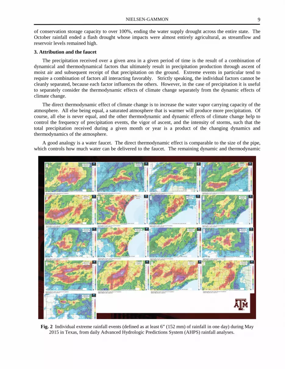
Fig. 2 Individual extreme rainfall events (defined as at least 6” (152 mm) of rainfall in one day) during May 2015 in Texas, from daily Advanced Hydrologic Predictions System (AHPS) rainfall analyses.

SCIENCE AND TECHNOLOGY INFUSION CLIMATE BULLETIN
10
effects are comparable to the handle of the faucet, which may be closed, slightly open, or fully open. The net resulting precipitation depends on both the size of the pipe and the position of the handle. However, when the handle is wide open, the precipitation intensity is controlled only by the size of the pipe.
Over the past 121 years, there is essentially no trend in springtime precipitation in Texas. If anthropogenic climate change has had an effect, it has been offset by natural variability. It is thus difficult to argue that climate change played a direct role in the record-setting May rainfall.
An upward trend does exist in intense one-day and two-day rainfall events in the south-central United States (e.g., Janssen et al. 2014). This means either that the precipitation handle is wide open more frequently, or that on days in which the precipitation handle is wide open, the atmosphere is delivering more precipitation. Since overall precipitation has not increased, we presume that the pipe has become wider rather than the handle position becoming more favorable. In other words, climate change is increasing the amount of precipitation on those days in which ideal intense precipitation conditions are present.
As for a possible interaction effect between natural variability and climate change, Wang et al. (2015) have found that global warming may have enhanced the atmospheric response to El Niño in Texas, which even without climate change favors enhanced springtime precipitation under developing El Niño conditions.
4. The pipe: Heavy rainfall events during May 2015
During May 2015, near-ideal intense precipitation conditions were present in various locations across Texas. On sixteen different days, some locations in Texas received at least six inches (152 mm) of rainfall (Fig. 2). These events occurred within every climate division of the state, and included major flooding events north of Fort Worth, along the Blanco River in Wimberly and San Marcos, and in parts of Houston. Individual events such of these appear to have been made more likely due to climate change.
5. Summary
With the lack of a positive trend in monthly springtime precipitation, there is no direct observational evidence that the record-setting May 2015 statewide rainfall total in Texas had an anthropogenic component. One study has found a possible enhancement of the springtime Texas rainfall response to El Niño. Much more apparent is the likely contribution of anthropogenic climate change to individual intense rainfall events within the month of May. This contribution is analogous to the effect of a wider pipe on water delivered by a faucet.
References
Janssen, E., D. J. Wuebbles, K. E. Kunkel, S. C. Olsen, and A. Goodman, 2014: Observational- and model-based trends and projections of extreme precipitation over the contiguous United States. Earth’s Future, 2, 99-113. doi: 10.1002/2013EF000185.
Wang, S.-Y. S., W.-R. Huang, H.-H. Hsu, and R. R. Gillies, 2015: Role of the strengthened El Niño teleconnection in the May 2015 floods over the southern Great Plains. Geophys. Res. Lett., 42, 8140-8146. doi: 10.1002/2015GL065211.

2. DROUGHT / PLUVIAL
40th NOAA Climate Diagnostics and Prediction Workshop

Science and Technology Infusion Climate Bulletin NOAA’s National Weather Service 40th NOAA Annual Climate Diagnostics and Prediction Workshop Denver, CO, 26-29 October 2015
______________
Correspondence to: Yen-Heng Lin, Department of Plants, Soils and Climate, Utah State University, Logan, UT; E-mail: [email protected]
California: Indications for Continued Groundwater Depletion after Drought and Causes of Drought Variety
S.-Y. Simon Wang12, Yen-Heng Lin1, Robert R. Gillies12, Kirsti Hakala3, and Lawrence E. Hipps1 1Department of Plants, Soils and Climate, Utah State University, Logan, UT
2Utah Climate Center, Utah State University, Logan, UT 3National Research Program, U.S. Geological Survey
ABSTRACT
California’s Central Valley is undergoing a groundwater drilling boom amid one of the most severe droughts in state history from 2012~2015. Within California’s Central Valley, home to one of the world’s most productive agricultural regions, drought and increased groundwater depletion occurs almost hand-in-hand but this relationship appears to have changed over the last decade. Data derived from 497 wells as variations of groundwater level (GW) have revealed a continued depletion of groundwater about one year after drought, a phenomenon that did not exist prior to year 2000 from the sliding correlation between PDSI and GW with a 15-year running window (Fig. 1). Possible causes include (a) lengthening of drought associated with amplification in the 4-6-year drought frequency since the late 1990s (Fig. 2), that drought conditions in California have become increasingly more intense and lasted longer (Cayan et al., 2010; MacDonald, 2010; Diffenbaugh et al., 2015), and (b) intensification of drought and increased pumping that enhances depletion, that Famiglietti (2014] noted that drought is the leading contributor to groundwater behavior, rather than changes in reservoir storage. Altogether, the implication is that groundwater storages in the Central Valley will likely continue to diminish even further in 2016, regardless of the drought status. This work has been accepted in Journal of Hydrometeorology (Wang et al., 2016).
Furthermore, as we know, upper-troposphere ridges play an important role to influence the
Fig. 1 Sliding correlations between the Central Valley PDSI and the groundwater level (GW) in the following year (year+1; solid line) and in the same year (year 0; dashed line), computed with a 15-year running window (one-sided). The LWET correlations with PDSI are indicated by thick circles for 2002-2014. Gray horizontal lines indicate the 99% confidence interval.
Fig. 2 Wavelet spectrum of the PDSI using the Morlet param-6 approach, in which the contour levels are chosen so that 75%, 50%, 25%, and 5% of the wavelet power are respectively above each level.

WANG ET AL.
13
drought in California (Wang et al. 2014), but each drought year has different climate regime. To understand the circulation variations within dry years, we applied the empirical orthogonal function (EOF) to depict the variation(s) of the Nov.~Mar. 250mb geopotential (Z250mb) high within the selected 18 dry winters. The results show that the first mode (Fig. 3a) and its Z250mb regression pattern with PC1 (Fig. 4a) is relative to the teleconnection varieties of Pacific North American (PNA) pattern (Fig. 4b) and the second mode (Fig. 3b) and its Z250mb regression pattern with PC2 (Fig. 4b) is relative to the negative North Pacific Oscillation (NPO) pattern (Fig. 4d). By comparing Z250mb (Figs. 4b and 4d) and PDSI (Figs. 5a and 5b) regression patterns with PNA and negative NPO, the variations of two dominated circulation patterns over Pacific Ocean, PNA and NPO, modulate the drought conditions in California. Nevertheless, the PNA and NPO variations do not directly cause the droughts.
References
Cayan, D. R., T. Das, D. W. Pierce, T. P. Barnett, M. Tyree, and A. Gershunov, 2010: Future dryness in the southwest US and the hydrology of the early 21st century drought. Proceedings of the National Academy of Sciences, 107(50), 21271-21276.
Diffenbaugh, N. S., D. L. Swain, and D. Touma, 2015: Anthropogenic warming has increased drought risk in California. Proceedings of the National Academy of Sciences, 112(13), 3931-3936.
Famiglietti, J. S., 2014: The global groundwater crisis. Nature Clim. Change, 4(11), 945-948.
MacDonald, G. M., 2010: Water, climate change, and sustainability in the southwest. Proceedings of the National Academy of Sciences, 107(50), 21256-21262.
Fig. 5 The boreal winter (Nov~Mar) PDSI regression patterns with (a) PNA and (b) negative NPO in 18 California dry years, superimposed with 95% significant test (hatch).
(a)
(b)
Fig. 3 (a) The first mode of EOF1 (shaded) of winter (Nov~Mar) Z(250mb) in 18 California dry years and its relative PC1, superimposed with these18 years’ mean ZE(250mb) . (b) The second mode.
Fig. 4 The Z250mb regression patterns in 18 California dry years with: (a) PC1 index (b) PNA index, (c) PC2 index, and (d) negative NPO index, superimposed with 95% significant test.

SCIENCE AND TECHNOLOGY INFUSION CLIMATE BULLETIN
14
Wang, S.-Y., L. Hipps, R. R. Gillies, and J.-H. Yoon, 2014: Probable causes of the abnormal ridge accompanying the 2013-14 California drought: ENSO precursor and anthropogenic warming footprint. Geophys. Res. Lett., 41, 3220-3226, doi: 10.1002/2014GL059748.
Wang, S.-Y., Y.-H. Lin, R. R. Gillies, and K. Hakala, 2016: Indications for protracted groundwater depletion after drought over the Central Valley of California. J. Hydrometeor., doi: 10.1175/JHM-D-15-0105.1, in press.

Science and Technology Infusion Climate Bulletin NOAA’s National Weather Service 40th NOAA Annual Climate Diagnostics and Prediction Workshop Denver, CO, 26-29 October 2015
______________
Correspondence to: Robert Burgman, AHC5-Ste 360, 12000 SW 8th Street, Department of Earth and Environment, Florida International University, Miami, FL 33199; E-mail: [email protected].
Simulated U.S. Drought Response to Interannual and Decadal Pacific SST Variability
Robert Burgman, Youkyoung Jang Department of Earth and Environment, Florida International University, Miami, FL
1. Introduction
Recent multiyear droughts in California and the Great Plains coincide with an extended period of arid conditions over much of the contiguous United States that began in 1999, with severe regional droughts occurring in 1999, 2002, 2006, 2008, and 2011. Understanding the mechanisms and probability for drought onset, persistence, and intensity is paramount for decision makers, who must assess potential impacts and management options. If there is long-term predictability for drought, the “memory” for this predictability resides with the global oceans, but precisely how the global oceans influence observed North American drought remains unresolved. In this study, we expand on previous studies by focusing on AGCM simulations where the decadal and interannual signals are effectively separated in order to examine how the cold phase Pacific SSTA patterns associated with different time scale variability impact hydroclimate over the contiguous United States, with a particular focus on the differences in amplitude of the equatorial and midlatitude SST anomalies and precipitation over the Great Plains region.
2. Models, modeling methodology, and data
Idealized AGCM simulations performed by members of the U.S. CLIVAR Drought Working Group (DWG) were used in this study. The low-frequency (LF) and high-frequency (HF) AGCM simulations of interest for this study were carried out by three of the five agencies that contributed AGCM data to the DWG in addition to the baseline simulations noted above. The three models are:
1. The NASA Global Modeling and Assimilation Office (GMAO) NSIPP, version 1 (NSIPP1) AGCM at 3° × 3.75°, L34 resolution (Bacmeister et al. 2000; Schubert et al. 2002).
2. The National Oceanic and Atmospheric Administration’s (NOAA) Climate Prediction Center Global Forecast System (GFS) AGCM at 2° × 2°, L64 resolution (Campana and Caplan 2005).
Fig. 1 The SST anomaly patterns (°C) used in forcing for experiments with principal components: (a) PcAn, (b) LFc, and (c) HFc. The top panels are the idealized anomaly patterns of each type and the bottom panels are the climatologically varying SSTs by years.

SCIENCE AND TECHNOLOGY INFUSION CLIMATE BULLETIN
16
3. NOAA’s Geophysical Fluid Dynamics Laboratory (GFDL) Atmosphere Model, version 2.1 (AM2.1), AGCM at 2° × 2.5°, L24 resolution (Delworth et al. 2006).
For the DWG AGCM simulations, idealized SST anomaly patterns are fixed in time and superimposed on climatologically varying SSTs derived from the Hadley Centre Sea Ice and Sea Surface Temperature dataset (HadISST; Rayner et al. 2003) for the period 1901–2004. The SST pattern for the Pacific (PcAn; Fig. 1a) comes from the baseline experiments. (See Schubert et al. 2009 for methodology and derivation of SST patterns). Note that the principal component (PC) time series associated with the PcAn pattern in Fig. 1a captures the interannual variability of ENSO in addition to variability on decadal time scales. The Drought Working Group also produced patterns of SST anomalies associated with the low-frequency (LF) and high-frequency (HF) tropical Pacific SST variability. The low-frequency cold (LFc) and high-frequency cold (HFc) patterns are shown in Figs. 1b and 1c, The patterns of the anomalies are similar in a broad sense (spatial correlations for PcAn and LFc, r = 0.93; PcAn and HFc, r = 0.9; and LFc and HFc, r = 0.79); however, the amplitude of the equatorial (midlatitude) anomalies differ by up to 1°C (0.3°C) between the different patterns. The GFDL AM2.1 and NASA NSIPP1 simulations were run for 50 yr and the NCEP GFS for 35 yr. For the purposes of the regional analysis in this study, the contiguous United States is divided into six subregions (see Fig. 2); the northern–southern western United States, the northern–southern Great Plains, and the northern–southern eastern United States.
3. Research highlights
Overall, there is agreement with previous results using the DWG model data, as all of the models simulated drought conditions over large portions of the contiguous United States for the La Niña–like PcAn SST forcing pattern. Building on previous results of the DWG, the current study finds differing levels of sensitivity to regional differences in prescribed Pacific SST forcing patterns with respect to internal atmospheric variability in the three AGCMs. The coherence of the AM2.1 responses for all forcing patterns and across all seasons (Fig 3a and d) suggests the model is overpredicting the strength of the tropical SST signal. Internal atmospheric variability and land–atmosphere interactions were shown to influence the GFS model response, though the shorter simulations also play a role in the reduced significance of the results presented (Fig. 3c and f). The SST forced response in the NSIPP1 AGCM (Fig 3b and e) is a function of the relative amplitude of the SST forcing in the tropics and middle latitudes, with detectible constructive interference between the two signals, similar to that seen between ocean basins (McCabe et al. 2004; Schubert et al. 2009). The current study points to a more significant role for the extratropical component of the SST in forcing the precipitation response; particularly over the western United States and northern Great Plains, via distinctly different teleconnections. In light of the results presented, it is certainly reasonable that the amplitude of the Pacific (PcAn) pattern dominated the drought response in the earlier works by the U.S. CLIVAR Drought Working Group (Schubert et al. 2009), when compared to the multidecadal Atlantic and warming trend patterns.
While the large equatorial component of the PcAn forcing may not be appropriate for comparison with the decadal- and century-scale Atlantic multidecadal oscillation (AMO) and global trend pattern, it is critical in the context of understanding the observed variability of the Pacific. The PcAn pattern can be seen as a “worst case” scenario for drought that is all the more relevant considering the recent occurrence of multiyear La Niña events (1998–2001, 2007–09, and 2010–12). The amplified response to the combined PcAn pattern seen in the NSIPP1 AGCM suggests that the severity of several recent droughts, particularly in the U.S.
Fig. 2 The regions of the United States used to form averages in Figs. 3 and 4

BURGMAN AND JANG
17
Southwest and Great Plains, is likely influenced by the combined cold decadal pattern that has prevailed since the late 1990s (Burgman et al. 2008, Clement et al. 2009) and the large number of individual La Niña events.
This work has been published in Journal of Climate in 2015.
References
Bacmeister, J., P. J. Pegion, S. D. Schubert, and M. J. Suarez, 2000: Atlas of seasonal means simulated by the NSIPP 1 atmospheric GCM. NASA Tech. Memo. 104606, Vol. 17, Goddard Space Flight Center, Greenbelt, MD, 194 pp.
Burgman, R. J., A. Clement, C. Mitas, J. Chen, and K. Esslinger, 2008: Evidence for atmospheric variability over the Pacific on decadal timescales. Geophys. Res. Lett., 35, L01704, doi:10.1029/2007GL031830
——, and Y. Jang, 2015: Simulated U.S. drought response to interannual and decadal Pacific SST variability. J. Climate, 28, 4688–4705, doi: http://dx.doi.org/10.1175/JCLI-D-14-00247.1
Campana, K., and P. Caplan, Eds., 2005: Technical procedures bulletin for the T382 Global Forecast System. Available online at http://www.emc.ncep.noaa.gov/gc_wmb/Documentation/TPBoct05/T382.TPB.FINAL.htm
Clement, A. C., R. Burgman, and J. R. Norris, 2009: Observational and model evidence for positive low-level cloud feedback. Science, 325, 460–464, doi:10.1126/science.1171255
Fig. 3 Annual mean (labeled MN in the top far left of each panel) and monthly precipitation climatology and simulated precipitation response with respect to control (PnAn) averaged over (a)–(c) the northern Great Plains and (d)–(f) the southern Great Plains. Model annual mean and monthly mean climatology is shown with dark blue bars for each case; and observed annual mean and monthly climatology are shown with light blue bars (right-hand side y axis; mm month−1). Annual mean and seasonal response of HFc (red), LFc (green), and PcAn (brown) compared to climatology control run. Solid circles indicate confidence at 90% (left-hand side y axis; mm day−1).

SCIENCE AND TECHNOLOGY INFUSION CLIMATE BULLETIN
18
Delworth, T. L., and Coauthors, 2006: GFDL’s CM2 global coupled climate models. Part I: Formulation and simulation characteristics. J. Climate, 19, 643–674, doi:10.1175/JCLI3629.1
McCabe, G. J., M. A. Palecki, and J. L. Betancourt, 2004: Pacific and Atlantic Ocean influences on multidecadal drought frequency in the United States. Proc. Natl. Acad. Sci. USA, 101, 4136–4141, doi:10.1073/pnas.0306738101
Rayner, N. A., D. E. Parker, E. B. Horton, C. K. Folland, L. V. Alexander, D. P. Rowell, E. C. Kent, and A. Kaplan, 2003: Global analyses of SST, sea ice, and night marine air temperature since the late nineteenth century. J. Geophys. Res., 108, 4407, doi:10.1029/2002JD002670
Schubert, S. D., and Coauthors, 2009: A U.S. CLIVAR project to assess and compare the responses of global climate models to drought-related SST forcing patterns: Overview and results. J. Climate, 22, 5251–5272, doi:10.1175/2009JCLI3060.1
Schubert, S. D., M. J. Suarez, P. J. Pegion, M. A. Kistler, and A. Kumer, 2002: Predictability of zonal means during boreal summer. J. Climate, 15, 420–434, doi:10.1175/1520-0442(2002)015<0420:POZMDB>2.0.CO;2

Science and Technology Infusion Climate Bulletin
NOAA’s National Weather Service
40th NOAA Annual Climate Diagnostics and Prediction Workshop
Denver, CO, 26-29 October 2015
______________
Correspondence to: Vasubandhu Misra, Department of Earth, Ocean and Atmospheric Science, Florida State University,
Tallahassee, FL; Email: [email protected]
Reconciling Seasonal Droughts and Landfalling Tropical Cyclones
in the Southeastern US
Vasubandhu Misra1,2,3
and Satish Bastola4
1Department of Earth, Ocean and Atmospheric Science, Florida State University, Tallahassee, FL
2Center for Ocean-Atmospheric Prediction Studies, Florida State University, Tallahassee, FL
3Florida Climate Institute, Florida State University, Tallahassee, FL
4School of Civil and Environmental Engineering, Georgia Institute of Technology, Atlanta, GA
ABSTRACT
A popular perception is that landfalling tropical
cyclones help to mitigate droughts in the Southeastern
United States (SeUS). However intriguing paradigms
on the role of large scale SST variations on continental
US including SeUS droughts and seasonal Atlantic
tropical cyclone activity confronts us. These paradigms
suggest that in the presence of warm (cold) eastern
tropical Pacific and cold (warm) Atlantic Ocean Sea
Surface Temperature Anomaly (SSTA) lead to the
increased likelihood of wetter (drier) conditions over
the continental US including the SeUS. Juxtaposing
this understanding with the fact that landfalling tropical
cyclones contribute significantly to the annual mean
total rainfall in the SeUS and in El Niño (La Niña)
years with cold (warm) tropical Atlantic SSTA lead to
reduced (increased) Atlantic tropical cyclone activity
raises a conflict on the role of the large-scale SST
variations in SeUS hydroclimate.
This study attempts to investigate the apparent
dichotomous role of the large scale SST variations on
the SeUS hydrology by examining the role of rainfall
from landfalling tropical cyclones in the SeUS to local
seasonal droughts (Figure 1).
This work has been published in Climate Dynamics
online on 14 May 2015.
Acknowledgements. This study was supported by
NOAA's Climate Program Office's Modeling, Analysis,
Predictions, and Projections program award
NA12OAR4310078
Reference
Misra, V. and S. Bastola, 2015: Reconciling droughts
and landfalling tropical cyclones in the
Southeastern United States. Clim. Dyn., in press, doi:10.1007/s00382-015-2645-7.
Fig. 1 a) The average drought index over the 28
watersheds spread across the southeastern
United States from the control model and
experimental model (where the rainfall for 5
days subsequent to landfall is removed) and
the difference in the drought index between
control and experiment, showing that the
mitigating impact of the landfalling TCs is
rather minimal, b) The drought index averaged
across all 28 watersheds for each year from
1954 to 2010 from control and experiment,
revealing apparent difference in months when
there are multiple landing TCs. (From Misra
and Bastola 2015).

Science and Technology Infusion Climate Bulletin
NOAA’s National Weather Service
40th NOAA Annual Climate Diagnostics and Prediction Workshop
Denver, CO, 26-29 October 2015
______________
Correspondence to: Kingtse C. Mo, 5830 University Research Court, Climate Prediction Center, NCEP/NWS/NOAA,
College Park, Maryland; E-mail: [email protected].
Flash Droughts over the United States
Kingtse C. Mo1 and Dennis P Lettenmaier
2
1Climate Prediction Center, NCEP/NWS/NOAA
2Department of Geography, University of California, Los Angeles, CA
Flash drought refers to relatively short periods of warm surface temperature and anomalously low and
rapid decreasing soil moisture (SM). Based on the physical mechanisms associated with flash droughts, we
classify these events into two categories: heat wave and precipitation (P) deficit flash droughts. We analyze
flash droughts based on observations of P, temperature (Tair), SM and evapotranspiration (ET) reconstructed
using four land surface models (VIC, Noah, Catchment and SAC) for the period 1916 to 2013. Both types of
flash droughts are manifested by SM deficits which cause damage to crops. Therefore, both are agricultural
droughts.
To determine the preferred regions for flash drought occurrence, we computed the frequency of
occurrence (FOC) by using a threshold method. We processed each model separately. For a given pentad T
and grid point x , we identified a flash drought event when a given definition of flash drought was met. That
pentad was defined as the onset. For each grid point, we computed the total number of pentads N under flash
drought of either type for the entire record for a given model. We defined the FOC as the percentage of
pentads under heat wave or P deficit flash droughts.
FOC (model) =
× 100%
where Ntotal is the total pentads.
The requirements for heat wave flash droughts are
Tair anomalies greater than one standard deviation (SD),
ET > 0 and SM% less than 40%. Figure 1a shows the
FOC for heat wave flash droughts. They occur most
often in the North Central, the Ohio Valley and the
Pacific Northwest. Heat wave flash droughts are resulted
from the confluence of severe warm air temperature and
low SM. The heat waves increase ET, and decrease SM.
Therefore, they tend to occur in the vegetation dense
areas.
The second type of flash droughts is caused by
precipitation deficits. We associate with lack of P, which
causes ET to decrease and temperature to increase. The
requirements for P deficit flash droughts are Tair > 1SD,
ET<0 and P <40%. Fig. 1b shows the FOC for P deficit
flash droughts. P deficit flash droughts are more common
than heat wave flash droughts. We find that P deficit
flash droughts are about twice as likely to occur as heat
wave flash droughts averaged over the conterminous U.S.
(CONUS). They are most prevalent over the southern
United States with maxima over the Southern Great
Plains and the Southwest, in contrast to heat wave flash
Fig. 1 FOC for (upper) the heat wave flash
droughts and (lower) the P deficit flash
droughts. The units are percentiles. Shadings
are given by the color bar. (Mo and
Lettenmaier 2015)

MO AND LETTENMAIER
21
droughts which are mostly likely to occur over the Midwest and the Pacific Northwest where the vegetation
cover is denser.
The P deficit drought is initialized by P deficits. The lack of P decreases SM. In the areas where SM and
ET anomalies have linear relationship, ET decreases. That leads to the increase of sensible heat and high
temperature. In this sense, high temperatures are the consequence of P deficits.
Acknowledgements. This project was supported by NOAA CPO MAPP Grant GC14-168A to the NOAA
Climate Prediction Center, and by NOAA Grant NA14OAR4310293 to the University of California, Los
Angeles.
References
Mo, K.C. and D.P. Lettenmaier, 2015: Heat wave flash droughts in decline. Geophy. Res Let. 42, doi: 10.1002
/2015GL06418.

Science and Technology Infusion Climate Bulletin NOAA’s National Weather Service 40th NOAA Annual Climate Diagnostics and Prediction Workshop Denver, CO, 26-29 October 2015
______________
Correspondence to: Parichart Promchote, Department of Plants, Soils, and Climate, Utah State University, 4820 Old Main Hill, Logan, UT 84322-4820; Email: [email protected]
The 2011 Great Flood in Thailand: Climate Diagnostics and Implications from Climate Change
Parichart Promchote1, S.-Y. Simon Wang1,2 , and Paul G. Johnson1 1Department of Plants, Soils, and Climate, Utah State University, Logan, UT
2Utah Climate Center, Utah State University, Logan, UT
ABSTRACT
Severe flooding occurred in Thailand during the 2011 summer season, which resulted in more than 800 deaths and affected 13.6 million people. The unprecedented nature of this flood in the Chao Phraya River Basin (CPRB) was examined and compared with historical flood years. Climate diagnostics were conducted to understand the meteorological conditions and climate forcing that lead to the magnitude and duration of this flood. Neither the monsoon rainfall nor the tropical cyclone frequency anomalies alone were sufficient to cause the 2011 flooding event. Instead, a series of abnormal conditions collectively contributed to the intensity of the 2011 flood: anomalously high rainfall in the pre-monsoon season especially during March; record-high soil moisture content thorough the year; elevated sea level height in the Gulf of Thailand which constrained drainage (Fig. 1(a)-(c)), as well as other water management factors. In the context of climate
Fig. 1 Monthly distribution of (a) rainfall computed from 1951-2013 for the CPRB, (b) soil moisture content couputed from 1948-2014 for the CPRB, and (c) sea level height computed from 1993-2013 for the Gulf of Thailand overlaid with 6 flood years. The above-normal values in 2011 are indicated by the yellow area. (d) Premonsoon (January-April) rainfall overlaid with the linear trend of the preriod 1980-2013 (red) and the 5-yr moving average (orange) for the CPRB. The linear trend slope is hightly significant with r2=0.32, p<0.01. (e) Premonsoon rainfall (normalized scales) derived from CMIP5 ensembles of GHG forcing superimposed with the 5-yr moving average (black) and post-1980 linear trend (orange) constructed for the CPRB. The linear trend slope is significant with r2=0.11, p<0.10. (f) Flood-period sea level height (July-December) overlaid with the linear trend constructed for the Gulf of Thailand. The linear trend slope is highly significant with r2=0.67, p<0.01.

PROMCHOTE ET AL.
23
change, the substantially increased pre-monsoon rainfall in CPRB after 1980 and the continual sea level rise in the river outlet (Fig. 1(d) and (f)) have both played a role. The rainfall increase is associated with a strengthening of the pre-monsoon northeasterly winds that come from East Asia. Attribution analysis using the Coupled Model Intercomparison Project Phase 5 historical experiments pointed to the anthropogenic greenhouse gases as the main external climate forcing leading to the rainfall increase (Fig. 1(e)). Together, these findings suggest increasing odds for potential flooding similar to the 2011 flood intensity.
This work has been published in Journal of Climate in 2015.
Reference
Promchote, P., S.-Y. Simon Wang, and P.G. Johnson, 2015: The 2011 Great Flood in Thailand: Climate Diagnostics and Implications from Climate Change. J. Climate, (in press), doi: 10.1175/JCLI-D-15-0310.1 .

3. DIAGNOSTICS ANDPREDICTION OF HIGHIMPACT EXTREME CLIMATEEVENTS
40th NOAA Climate Diagnostics and Prediction Workshop

Science and Technology Infusion Climate Bulletin NOAA’s National Weather Service 40th NOAA Annual Climate Diagnostics and Prediction Workshop Denver, CO, 26-29 October 2015
______________
Correspondence to: Qin Zhang, 5830 University Research Court, Climate Prediction Center, NOAA/NWS/NCEP, College Park, Maryland; E-mail: [email protected].
New Measure of Forecast Uncertainty for the North American Multi-Model Ensemble
Qin Zhang1, Yuejian Zhu2, Hong Guan2,5 , Jon Gottschalck1, Jin Haung1, Huug van den Dool1, Emily Becker1,3, and Li-Chuan Chen1,4
1Climate Prediction Center, NOAA/NWS/NCEP, College Park, MD 2Environmental Modeling Center, NCEP/NWS/NOAA, College Park, MD
3Innovim, LLC., Greenbelt, MD 4Earth System Science Interdisciplinary Center/Cooperative Institute for Climate and Satellites,
University of Maryland, College Park, MD 5System Research Group Inc, Colorado Springs, CO
ABSTRACT
Since August 2011, realtime monthly and seasonal forecasts from the North American Multi-Model Ensemble (NMME) have been made every month by the NCEP Climate Prediction Center (CPC). Among the most popular NMME products, NMME ensemble mean maps are made from the equally weighted average of the participating models’ ensemble means, after removing systematic errors. However, some users are interested in how the models are different – that is, the diversity of the forecasts. In this study, we defined a normalized spread (SPRnor) to measure NMME forecast uncertainty, which is calculated from the multi-model predictive variance (including between-model variance and within-model variance) and then normalized by the observed standard deviation. When SPRnor is smaller than 1, it indicates the NMME forecast has less uncertainty, since the models are in good agreement over the grid point. When SPRnor is greater than 1, it means that the NMME forecast uncertainty is larger than the observed inter-annual variability, as the model forecasts are more dispersed. Generally, the SPRnor grows with the forecast leading time, and also varies with season. Therefore, we supply normalized spread maps to complement the NMME ensemble mean forecast and give users additional information of NMME forecast uncertainty in realtime.
1. Introduction
More and more users have gone to the North American Multi-Model Ensemble web page (http://www.cpc.ncep.noaa.gov/products/NMME/) to view NMME products for their operational missions and applications since the first NMME seasonal and monthly prediction was made in August 2011 (Kirtman et al. 2014). Among the thousands of uploaded figures of realtime prediction for both North American and global domains, the most popular products are the NMME mean 2m temperature and precipitation anomalies made by the equally weighted average of each NMME model’s ensemble mean, after removing systematic errors. However, the information from the NMME ensemble mean anomalies is not enough, since it is akin to a deterministic forecast. Users are also interested in how the forecasts for each model differ and the confidence of the NMME prediction. While the NMME probability forecasts, calculated from all ensemble members with equal weights, have been made each month (Becker et al. 2014) since 2012, their weights are not completely consistent with the maps of NMME anomalies. Therefore, the motivation of this work is to define and develop new products to express the prediction uncertainty of NMME and indicate the model forecast diversity.

SCIENCE AND TECHNOLOGY INFUSION CLIMATE BULLETIN
26
2. Definition of the spread for multi-model ensemble
The NMME is a dynamic multi-model ensemble forecast system, initially comprised of 6 US models (CFSv1 & CFSv2/NCEP, ECHAM-a & ECHAM-f/IRI, NCAR-CCSM3/COLAR-UM, GFDL-CM2.1, and GEOS5/NASA). For the past two years, the NMME has included seven models: two Canadian models (Can-CM3&4) (Environment Center of Canada joined in August 2012, when CFSv1 was retired), two models from GFDL, GEOS5/NASA, CFSv2/NCEP, and NCAR-CCSM4 (which replaced NCAR-CCSM3). All of the NMME models are atmosphere-ocean coupled, and the horizontal resolution of the exchanged variables is 1x1 degree, consistent with the retrospective forecasts from 1982 to 2010. The NMME model climatologies are calculated from the 29 years of retrospective forecasts to remove systematic bias in the mean at each leading forecast time for each model before calculating the NMME ensemble mean. The model’s prediction skills (as expressed by the anomaly correlation) are also obtained from these retrospective forecasts.
We define the multi-model ensemble predictive variance in space (s) and time (t), lead (τ) and IC month (m) for an anomalous field, according to Raftery (1993):
))''(1
(1
)''(1
1
2
11
2 ∑∑∑===
−+−=N
nkkn
K
k
K
kk Ff
NKFF
KVAR (1)
where Fk’ is the kth model ensemble mean anomaly after mean bias correction. F’ is the equal weight averaged NMME ensemble mean for (K=7) models and fnk’ is the anomaly of each member for each model, as N is the number of the members for each model. VAR is a function of space, time, forecast lead and either the start month or the target month.
Here the predictive variance should be the sum of the two terms. One (the first term) is the between-model variance, another one (the second term) is the within-model variance. The between-model variance is the distance of the 7 individual model ensemble means from the multi-model ensemble mean, and the within-model variance is the average distance of each model member from its model’s ensemble mean. (Raftery, et al. 2005).
The spread of NMME also consists of two terms:
SPR2 = VAR = SPR2 ensm + SPR2 memb (2)
where the first term represents the diversity of the models’ ensemble means relative to the forecast signal (we call it ensemble mean spread). The second term is the spread of the individual members relative to their models’ ensemble means, which is linked to the forecast noise (hereafter called member spread).
2
1
2 )''(1
FFK
ensmSPR k
K
k
−= ∑=
(3)
))''(1
(1
1 1
22 ∑ ∑= =
−=K
k
N
nknk Ff
NKmembSPR (4)
Fig. 1 Spread (black solid line) of Nino3.4 for NMME hindcasts (1982-2010) and the ensemble mean spread (SPRensm, dashed line) and the members of spread (SPRmemb, dotted line) with the spreads of individual model (color lines).

ZHANG ET AL.
27
We also normalized the NMME spread to eliminate spatial and seasonal variation. Normalized multi-model ensemble mean spread indicates the uncertainty of the NMME ensemble mean prediction or the model forecast diversity. It is also known as the "envelope of solutions" for each lead forecast time. We define the normalized spread as a ratio of the root mean square of predictive variance to the observed standard deviation (STD), that is,
obsSTDVARSPRnor /)( 2/1= (5)
When SPRnor is smaller than 1, it indicates the NMME forecast has less uncertainty since the models are in good agreement over the grid point. When SPRnor is greater than 1, it means that the NMME forecast has more uncertainty than observed inter-annual variability due to the greater dispersion of model forecasts.
3. Results
a. The relationship of spread and the forecast uncertainty
Among the most popular NMME figures are the Nino3.4 plumes (Barnston et al. 2015). These show 7-month lead Nino3.4 index forecasts for the individual members and the ensemble mean of each model, as well as the equally weighted NMME ensemble mean (see http://www.cpc.ncep.noaa.gov/products/NMME/current/plume.html). The Nino3.4 plumes also show the forecast uncertainty visually: the denser the member distribution the higher the prediction probability. Here we describe the relationship of the NINO3.4 spread and forecast uncertainty by using 29 years of NMME retrospective forecasts as an example.
Figure 1 shows the SPR of NMME Nino3.4 index (black solid line) and its two component terms, the NMME ensemble mean spread (SPRensm, labeled Model_ENS, dashed line) and the spread of all members (SPRmemb, labeled Model_MEAN, dotted line) with the individual models’ spread (colored lines). All of these quantities grow with forecast lead time. However, the NMME ensemble mean spread (SPRensm) reaches saturation after 4 lead months and increases slowly after. The spread of NMME is bigger than that of any individual model, indicating that the ensemble mean of NMME covers all members and have a wide PDF for the all kind of predictability from the individual model.
Fig. 2 Spread of NMME calculated for each month from hindcasts (1982-2010).
Fig. 3 Realtime forecast of Nino3.4 plumes with the NMME spread in shading for Oct. 2015 IC.

SCIENCE AND TECHNOLOGY INFUSION CLIMATE BULLETIN
28
From figure 2, we find that the spread of NMME not only increases with forecast lead time but also varies with the season of initial forecast time (IC). The biggest peak of forecast uncertainty is for spring initial conditions, corresponding to the well- known “spring barrier” of ENSO prediction. The smallest spread (highest forecast confidence) is for forecasts made in the fall (September), when ENSO predictive probability is high, especially within 4 months lead.
Figure 3 shows the realtime forecast of Nino3.4 plumes, with NMME spread in shading, for October 2015 initial conditions. It is easy to see that the spread is consistent with the diversity of the ensemble mean of NMME models on the occasion.
b. Normalized NMME spread
Since the spread varies spatially and temporally, the multi-model spread calculated from formula (2) is hard to compare to the model forecast diversity in a different location or time. For the maps of NMME prediction, we normalize the spread by formula (5) to extract the information of NMME forecast diversity. Figs. 4 and 5 show NMME realtime prediction of 2m temperature and precipitation anomalies (contours) with normalized spread (shading) for North America for October 2015 initial conditions.
The NMME predicts warmer-than-average temperatures over the western half of North America, partially influenced by El Niño developing in the fall of 2015. Forecasts from the NMME models are more consistent in this region than in the south-eastern CONUS, where the forecast has higher uncertainty, shown by the models’ prediction diversity. On the other hand, the forecast for positive precipitation anomalies over the eastern CONUS has less uncertainty than that over the western US (Fig. 5). The normalized spread gives users information about how NMME model forecasts differ, or the diversity in the predictions.
4. Summary and discussion
NMME realtime spread is defined as the multi-model ensemble predictive variance, including between-model variance and within-model variance. Normalized ensemble spread is a new
Fig. 4 NMME realtime prediction of 2m temperature anomalies (contours) with normalized spread (shading) of North America for October 2015 initial conditions.
Fig. 5 NMME realtime prediction of precipitation anomalies (contours) with normalized spread (shading) of the North America for October 2015 initial conditions.

ZHANG ET AL.
29
measurement for NMME forecast uncertainty, consistent with the forecast of NMME ensemble mean anomalies. SPRnor ≤ 1 indicates the model forecasts are in good agreement over the grid points. SPRnor > 1 means that the model forecasts are more dispersed, and therefore have more uncertainty, than observed inter-annual variability. In generally, realtime SPRnor increases with forecast lead time. However, some variables, such as precipitation, may be influenced by seasonal variance in certain regions.
References
Barnston, A.G., M.K. Tippett, H.M. van den Dool, and D.A. Unger, 2015: Toward an improved multimodel ENSO prediction. J. Appl. Meteor. Climatol., 54, 1579–1595. doi: http://dx.doi.org/10.1175/JAMC-D-14-0188.1
Becker, E., H.M. van den Dool, Q. Zhang, 2014: Predictability and forecast skill in NMME. J. Climate, 27, 5891–5906. doi: http://dx.doi.org/10.1175/JCLI-D-13-00597.1
Kirtman, B.P., and Coauthors, 2014: The North American Multi-Model Ensemble (NMME): Phase-1 seasonal to interannual prediction, phase-2 toward developing intra-seasonal prediction. Bull. Amer. Meteor. Soc., 95, 585–601. http://dx.doi.org/10.1175/BAMS-D-12-00050.1
Raftery, A.E., 1993: Bayesian model selection in structural equation models. Testing Structural Equation Models, K.A. Bollen and J.S. Long, Eds., 163–180.
Raftery, A.E., T. Gneiting, F. Balabdaoui, and M. Polakowski, 2005: Using Bayesian model averaging to calibrate forecast ensembles. Mon. Wea. Rev., 133, 1155–1174.

Science and Technology Infusion Climate Bulletin
NOAA’s National Weather Service
40th NOAA Annual Climate Diagnostics and Prediction Workshop
Denver, CO, 26-29 October 2015
______________
Correspondence to: Emily J. Becker, 5830 University Research Court, Climate Prediction Center, NOAA/NWS/NCEP,
College Park, Maryland; E-mail: [email protected].
Forecasting Temperature Extremes with
the North American Multi-Model Ensemble (NMME)
Emily J. Becker1,2
, Huug van den Dool1, Qin Zhang
1, Li-Chuan Chen
1,3
1Climate Prediction Center, NOAA/NWS/NCEP, College Park, Maryland 2Innovim LLC, Greenbelt, Maryland
3Earth System Science Interdisciplinary Center, University of Maryland, College Park, MD
This study examines the forecast skill of 2 m temperature extremes in the monthly mean (T2m),
maximum (Tmax), and minimum (Tmin) using the North American Multi-Model Ensemble (NMME;
Kirtman et al. 2014), an ensemble of state-of-the-art coupled global climate models. Extremes are where the
real impact of weather and climate are felt, yet there are
currently very few forecasts for short-term climate
extremes (STCE). Aggregate skill (as assessed using the
anomaly correlation) for forecasts of STCE only has
previously been found to be higher than the aggregate
skill of all forecasts (Becker et al. 2013), providing
confidence that a useful forecast for STCE might be
possible.
The NMME currently provides real-time guidance
for NOAA’s operational short-term climate forecasts,
and includes a database of retrospective forecasts (1982-
2010), used for bias correction, calibration, and skill
studies. Seven models from the NMME contribute to
this study: NCEP-CFSv2, Environment Canada’s
CanCM3 and CanCM4, GFDL’s CM2.1 and FLOR,
NASA-GEOS5, and NCAR-CCSM4. A new maximum
and minimum temperature dataset was recently created
at CPC, and is interpolated to the NMME grid and
timescale to allow for an initial assessment of these
fields. The aggregate skill of deterministic forecasts of
Tmax and Tmin in general is found to be slightly lower
in magnitude to that of 2 m temperature, with some
differences in geography.
Temperature extremes are herein defined as the top
and bottom decile (10%) of the historical record at each
gridpoint, using the 1982-2010 hindcasts, with cross-
validation. A Gaussian distribution is assumed, but may
not be the most accurate fit; this is a point that requires
further examination. This study assesses forecast
verification, that is, the question of “did the forecast
come true?” using deterministic forecasts, at a one-month
lead for the monthly mean, over all initial conditions.
Area-average skill is assessed using the anomaly
correlation. When assessing the skill at individual
gridpoints, the Symmetric Extremal Dependence Index
Fig. 1 Anomaly correlation for monthly-mean 2 m
temperature (top) and minimum temperature
(bottom), area-aggregated over North
America, for the seven individual NMME
models’ ensemble means and the NMME
grand ensemble mean, averaged over all 12
initial conditions. Gray bars show anomaly
correlation for all forecasts, and orange
indicates the upper decile, i.e. positive
extremes.

BECKER ET AL.
31
(SEDI; Ferro and Stevenson 2011) which is non-degenerate for rare events, is employed. The decile definition
of extremes results in approximately 35 “extreme” events per gridpoint over all 12 initial months for 29 years
of retrospective forecasts.
The previous finding of higher anomaly correlation for forecasts of extremes is confirmed (Fig. 1). Skill
for forecasts of extremes of mean 2 m temperature (both negative and positive extremes) is slightly higher
than extremes in Tmax and Tmin. Overall, Tmin is predicted slightly more skillfully than Tmax, especially
when positive extremes are examined. Tmin has been more affected by the warming trend over the past
several decades, which may in part explain this difference. Forecasts for positive extremes of all three
temperatures are highest over the northern tier of North America, where they are generally >30% better than a
climatological forecast (Fig. 2).
This is a preliminary study that demonstrates that there is some potential for skillful forecasting of
extremes. Further experimentation will examine the definition of “extreme”, including possible use of
absolute temperature thresholds and consideration of warm-season positive Tmax extremes and cold-season
negative Tmin extremes. A large ensemble such as the NMME is valuable in constructing probabilistic
forecasts, and further analysis will be necessary to discover valid thresholds for triggering an extreme forecast.
Acknowledgements. We gratefully acknowledge the usage of the NMME Phase 1 and 2 data. The NMME
Project and data dissemination is supported by NOAA, NSF, NASA and DOE. We thank the climate
modeling groups for producing and making available their model output. NOAA NCEP, NOAA Climate Test
Bed and NOAA Climate Program Office jointly provide coordinating support and the NMME data archives
are maintained by IRI and NCAR.
References
Becker, E. J., H. van den Dool, and M. Pena, 2013: Short-term climate extremes: Prediction skill and
predictability. J. Climate, 26, 512-531.
Ferro, Christopher A. T. and David B. Stephenson, 2011: Extremal Dependence Indices: Improved
verification measures for deterministic forecasts of rare binary events. Wea. Forecasting, 26, 699–713.
doi: http://dx.doi.org/10.1175/WAF-D-10-05030.1
Kirtman, B. P., D. Min, J. M. Infanti, J. L. Kinter, D. A. Paolino, Q. Zhang, H. van den Dool, S. Saha, M. P.
Mendez, E. Becker, P. Peng, P. Tripp, J. Huang, D. G. DeWitt, M. K. Tippett, A. G. Barnston, S. Li, A.
Rosati, S. D. Schubert, Y.-K. Lim, Z. E. Li, J. Tribbia, K. Pegion, W. Merryfield, B. Denis and E. Wood,
2014: Phase-1 seasonal to interannual prediction, phase-2 toward developing intra-seasonal prediction.
Bull. Amer.Meteor. Soc., 95, 585–601. doi:10.1175/BAMS-D-12-00050.1.
Fig. 2 Symmetric Extremal Dependence Index (SEDI) for upper-decile (left) and lower-decile (right)
forecasts of monthly-mean maximum temperature, averaged over all 12 initial months.

Science and Technology Infusion Climate Bulletin NOAA’s National Weather Service 40th NOAA Annual Climate Diagnostics and Prediction Workshop Denver, CO, 26-29 October 2015
______________
Correspondence to: Flavio Lehner, Climate and Global Dynamics Division, National Center for Atmospheric Research, Boulder, CO; E-mail: [email protected].
Detection and Attribution of Extreme Temperature Using an Analogue-based Dynamical Adjustment Technique
Flavio Lehner1, Clara Deser1, Laurent Terray2 1Climate and Global Dynamics Division, National Center for Atmospheric Research, Boulder, CO, USA
2Sciences de L’Univers au CERFACS, URA-1875, CERFACS/CNRS, Toulouse, France
1. Introduction
Recent studies have highlighted the importance of internal variability in decadal trends and variability of regional-scale temperature and precipitation (Deser et al. 2012; Hawkins et al. 2015). Understanding and potentially reducing the uncertainties in climate change projections arising from internal variability has been a focal point of climate research over the last decade (Bindoff et al. 2013). The superposition of anthropogenically forced climate change with this unforced internal variability complicates attempts to detect and attribute climate change (Thompson et al. 2009). In the Northern Hemisphere mid to high latitudes, the stochastic variability of atmospheric circulation is a major contributor to this internal variability (Smoliak et al. 2015; Deser et al. 2015). Beyond decadal trends in temperature or precipitation, recent research has focused on diagnosing the driving factors behind individual extreme events, such as heat waves, cold snaps, or floods (Herring et al. 2015). It is therefore of interest to estimate the contribution of atmospheric circulation to a given trend or anomaly in temperature or precipitation.
Here we present a new method, based on constructed analogues, to estimate the contribution of atmospheric circulation to a given surface temperature anomaly. The details and an application to decadal temperature trends are described in Deser et al. 2015. The paper here is structured as follows. Section 2 summarizes the new method and introduces the data it is applied to. Section 3 illustrates how this method can be used to diagnose high temperature events. Section 4 summarizes these results and provides an outlook onto ongoing and future projects.
2. Data and methodology/experimental design
a. Dynamical adjustment of temperature
To estimate the contribution of atmospheric circulation to surface air temperature (SAT) changes, we apply a dynamical adjustment technique based on constructed circulation analogues. A full description of the methodology is given in Deser et al. 2015, of which we provide a summary here.
The method aims at empirically determining the component of SAT variability that arises solely from atmospheric circulation changes, characterized here by sea level pressure (SLP). This component is termed the ‘dynamical contribution’ to temperature variability. Subtracting the dynamical contribution from the raw field yields the residual, which is to first order an estimate of the ‘thermodynamical contribution’.
In practice, for a given target month, e.g., July 2015, we looking through all other available Julys in a given record, searching for Julys which have an analogues SLP pattern to the target month. The closest analogues are determined by finding the smallest Euclidean distance from the SLP pattern of the target month. Among the closest 80 analogues we randomly choose 50. An optimal linear combination of the 50 analogues is then computed that best fits the SLP pattern of the target month. Using the linear coefficients determined this way, we construct a SAT anomaly field that is defined as the optimal linear combination of the SAT anomalies associated with the SLP analogues. The process of randomly selecting 50 out of 80 analogues and constructing a best fit pattern is repeated 100 times to get an upper bound on the thermodynamically-induced internal variability. We then average over the 100 sets of SLP analogues and associated SAT anomalies to

LEHNER ET AL.
33
arrive at a best estimate of dynamically induced SAT anomalies for the target pattern. This dynamic contribution can then be subtracted from the target SAT field, yielding a dynamically adjusted field. The whole procedure is applied analogously to all months available, so that eventually all monthly mean SAT fields in a given record are dynamically adjusted. Prior to the whole analysis, the SAT time series is detrended with a quadratic fit to remove the global warming signal (see Deser et al. 2015 for details). The dynamical adjustment is applied to the following model simulations and observational datasets.
b. Model simulations and observations
We use monthly mean output from the Large Ensemble with the fully coupled Community Earth System Model 1, hereafter CESM LE (Kay et al. 2015). The CESM LE is an ensemble of 30 simulations from 1920 to 2100, in which each simulation was started from slightly different atmospheric initial conditions, while using the same ocean initial conditions. In accordance with protocols from the Coupled Model Intercomparison Project 5 (CMIP5; Taylor et al. 2012), historical natural and anthropogenic forcing was applied from 1920 to 2005 and the Representative Concentration Pathway 8.5 (RCP 8.5) thereafter. Due to its size, the Large Ensemble allows us to sample internal variability in a robust manner, as will be shown in Section 3b.
For observations we use monthly mean SAT from MLOST (Vose et al. 2012) and SLP from the Twentieth Century Reanalysis (Compo et al. 2011).
3. Results
a. Application to observed high temperature events
We pick two examples from observations to illustrate the dynamical adjustment method: the exceptionally warm July over the US in 1980 and the exceptionally warm August over central Europe in 2003.
Fig. 1a shows the raw SAT anomaly of July 1980, relative to its 1951-1980 climatology, as well as the corresponding SLP. During this month, a strong and persistent heatwave took hold of large parts of the Midwestern US, with SAT anomalies of over 5°C. Fig. 1b shows the dynamical contribution to the SAT field in Fig. 1a as determined by the dynamical adjustment method. The SLP pattern in Fig. 1b is the analogue constructed from similar July SLP patterns in the observational record. There is good agreement of this pattern with the SLP pattern in Fig. 1a, indicating that the dynamical adjustment is successful in constructing analogues patterns (the residual/”error” is given in Fig. 1c). The SAT anomalies in Fig. 1b are then the constructed SAT field, i.e., the SAT anomalies that typically go along
Fig. 1 (a) July 1980 surface air temperature (SAT; shading) and sea level pressure (SLP; contours, in 1 hPa increments starting at +/− 0.5 hPa) anomalies from their 1951-1980 climatology. (b) Dynamical contribution of constructed SLP pattern (contours) to SAT anomalies (shading). (c) Thermodynamic contribution to SAT anomalies (shading) and difference between true and constructed SLP anomalies (contours) as residual from subtracting (b) from (a). (d-f) Same as (a-c), but only SAT anomalies >2σ are shown. The spatial mean over the gray box is given in the bottom left corner with the fraction of the mean in panel (d).
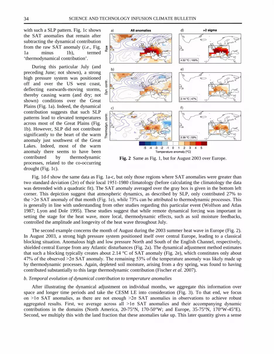
SCIENCE AND TECHNOLOGY INFUSION CLIMATE BULLETIN
34
with such a SLP pattern. Fig. 1c shows the SAT anomalies that remain after subtracting the dynamical contribution from the raw SAT anomaly (i.e., Fig. 1a minus 1b), termed ‘thermodynamical contribution’.
During this particular July (and preceding June; not shown), a strong high pressure system was positioned off and over the US west coast, deflecting eastwards-moving storms, thereby causing warm (and dry; not shown) conditions over the Great Plains (Fig. 1a). Indeed, the dynamical contribution suggests that such SLP patterns lead to elevated temperatures across most of the Great Plains (Fig. 1b). However, SLP did not contribute significantly to the heart of the warm anomaly just southwest of the Great Lakes. Indeed, most of the warm anomaly there seems to have been contributed by thermodynamic processes, related to the co-occurring drought (Fig. 1c).
Fig. 1d-f show the same data as Fig. 1a-c, but only those regions where SAT anomalies were greater than two standard deviation (2σ) of their local 1951-1980 climatology (before calculating the climatology the data was detrended with a quadratic fit). The SAT anomaly averaged over the gray box is given in the bottom left corner. This depiction suggest that atmospheric dynamics, as described by SLP, only contributed 27% to the >2σ SAT anomaly of that month (Fig. 1e), while 73% can be attributed to thermodynamic processes. This is generally in line with understanding from other studies regarding this particular event (Wolfson and Atlas 1987; Lyon and Dole 1995). These studies suggest that while remote dynamical forcing was important in setting the stage for the heat wave, more local, thermodynamic effects, such as soil moisture feedbacks, controlled the amplitude and longevity of the heat wave throughout July.
The second example concerns the month of August during the 2003 summer heat wave in Europe (Fig. 2). In August 2003, a strong high pressure system positioned itself over central Europe, leading to a classical blocking situation. Anomalous high and low pressure North and South of the English Channel, respectively, shielded central Europe from any Atlantic disturbances (Fig. 2a). The dynamical adjustment method estimates that such a blocking typically creates about 2.14 °C of SAT anomaly (Fig. 2e), which constitutes only about 47% of the observed >2σ SAT anomaly. The remaining 53% of the temperature anomaly was likely made up by thermodynamic processes. Again, depleted soil moisture, arising from a dry spring, was found to having contributed substantially to this large thermodynamic contribution (Fischer et al. 2007).
b. Temporal evolution of dynamical contribution to temperature anomalies
After illustrating the dynamical adjustment on individual months, we aggregate this information over space and longer time periods and take the CESM LE into consideration (Fig. 3). To that end, we focus on >1σ SAT anomalies, as there are not enough >2σ SAT anomalies in observations to achieve robust aggregated results. First, we average across all >1σ SAT anomalies and their accompanying dynamic contributions in the domains (North America, 20-75°N, 170-50°W; and Europe, 35-75°N, 170°W-45°E). Second, we multiply this with the land fraction that these anomalies take up. This later quantity gives a sense
Fig. 2 Same as Fig. 1, but for August 2003 over Europe.

LEHNER ET AL.
35
of SAT anomaly amplitude and spatial extent (hereafter called ‘anomaly magnitude’). The following examples are based on boreal summer means (June-August).
In North America the period 1930-1940 (the “Dust Bowl” era) was marked by exceptional anomaly magnitudes, which are not reproduced by any of the ensemble members of CESM LE (Fig. 3a), indicating that the model is lacking a process or additional forcing that would be crucial for the generation of such anomaly magnitudes. Previous model studies found that specifying additional dust emissions from land use change and drought during that period improves the agreement with observations (Cook et al. 2008). Still, the dynamical adjustment suggests a significant contribution from dynamics during 1930-1940, originating from a persistent high pressure ridge over the Western US, as identified by other studies (Brönnimann et al. 2009). Averaged over the period 1920-1980 the partitioning between dynamic and thermodynamic contributions to >1σ anomaly magnitudes is about 50% each in both observations (47% vs. 53%) and CESM (50% vs. 50%). After 1980, the model’s forced response (the ensemble mean) shows an increase in anomaly magnitudes, largely driven by an increase of the thermodynamic contribution, which constitutes the fingerprint of radiative forcing from increasing greenhouse gas concentrations.
The European domain is smaller and on average has a larger contribution from dynamics during 1920-1980 (57% in observations, 66% in CESM). After 1980, Europe shows a very similar behavior as North America with increasing anomaly magnitudes, mainly driven by an increase in the thermodynamic contribution. The summer of 2003 as a whole, taking into account June and July in addition to August (Fig. 2), shows a large thermodynamic contribution in observations.
4. Summary and outlook
In this study we applied a new method that estimates the dynamically induced variability from a surface air temperature field using constructed circulation analogues (Deser et al. 2015). It is shown that the method can be used to diagnose drivers of a given temperature anomaly in observations, but also help to understand the dynamic and thermodynamic contributions to anthropogenically driven climate change in model simulations.
The CESM LE shows skill in reproducing the partitioning between dynamic and thermodynamic contributions of high summer temperatures as suggested by observations, namely about 50% each for the period prior to 1980 over North America. A notable exception is the Dust Bowl era, which in its amplitude and spatial extent is not reproduced by any of the CESM simulations.
Diagnosing other climate variables, such as precipitation, or events on shorter time scale, such as heat waves, constitute promising future avenues of this method.
Fig. 3 Time series of anomaly magnitude of >1σ events, averaged from June through August (see text for details) for (a) North America and (b) Europe and the relative contribution from dynamics. Bold lines are observations, while thin lines and shading are the CESM LE ensemble mean and minimum-maximum range across the ensemble, respectively. Gaps in observations indicate that there occurred no >1σ event in that particular summer over the respective domain.
SCIENCE AND TECHNOLOGY INFUSION CLIMATE BULLETIN
36
References
Bindoff, N., and Coauthors, 2013: Detection and attribution of climate change: from global to regional. Climate Change 2013: The Physical Science Basis. Contribution of Working Group I to the Fifth Assessment Report of the Intergovenermnetal Panel on Climate Change.
Brönnimann, S., and Coauthors, 2009: Exceptional atmospheric circulation during the “Dust Bowl”. Geophys. Res. Lett., 36, 1–6. doi:10.1029/2009GL037612.
Compo, G. P., and Coauthors, 2011: The Twentieth Century Reanalysis Project. Q. J. R. Meteorol. Soc., 137, 1–28. doi:10.1002/qj.776.
Cook, B. I., R. L. Miller, and R. Seager, 2008: Dust and sea surface temperature forcing of the 1930s “Dust Bowl” drought. Geophys. Res. Lett., 35, 1–5. doi:10.1029/2008GL033486.
Deser, C., R. Knutti, S. Solomon, and A. S. Phillips, 2012: Communication of the role of natural variability in future North American climate. Nat. Clim. Chang., 2, 775–779. doi:10.1038/nclimate1562.
——, L. Terray, and A. S. Phillips, 2016: Forced and internal components of winter air temperature trends over North America during the past 50 years: Mechanisms and implications. J. Climate, e-view. doi: 10.1175/JCLI-D-15-0304.1
Fischer, E. M., S. I. Seneviratne, P. L. Vidale, D. Lüthi, and C. Schär, 2007: Soil moisture-atmosphere interactions during the 2003 European summer heat wave. J. Climate, 20, 5081–5099, doi:10.1175/JCLI4288.1.
Hawkins, E., R. S. Smith, J. M. Gregory, and D. A. Stainforth, 2015: Irreducible uncertainty in near-term climate projections. Clim. Dyn. doi:10.1007/s00382-015-2806-8.
Herring, S. C., M. P. Hoerling, J. P. Kossin, T. C. Peterson, and P. A. Stott, Eds., 2015: Explaining extreme events of 2014 from a climate perspective. Bull. Amer. Meteor. Soc., 96 (12), S1–S172.
Kay, J. E., and Coauthors, 2015: The Community Earth System Model (CESM) Large Ensemble Project: A community resource for studying climate change in the presence of internal climate variability. Bull. Amer. Meteor. Soc., 96, 1333–1349.
Lyon, B., and R. M. Dole, 1995: A diagnostic comparison of the 1980 and 1988 US summer heat wave- droughts. J. Climate, 8, 1658–1675. doi:10.1175/1520-0442(1995)008<1658:ADCOTA>2.0.CO;2.
Smoliak, B. V., J. M. Wallace, P. Lin, and Q. Fu, 2015: Dynamical adjustment of the Northern Hemisphere surface air temperature field: Methodology and application to observations. J. Climate, 28, 1613–1629. doi:10.1175/JCLI-D-14-00111.1.
Taylor, K. E., R. J. Stouffer, and G. a. Meehl, 2012: An overview of CMIP5 and the experiment design. Bull. Am. Meteorol. Soc., 93, 485–498. doi:10.1175/BAMS-D-11-00094.1.
Thompson, D. W. J., J. M. Wallace, P. D. Jones, and J. J. Kennedy, 2009: Identifying signatures of natural climate variability in time series of global-mean surface temperature: Methodology and insights. J. Climate, 22, 6120–6141. doi:10.1175/2009JCLI3089.1.
Vose, R. S., and Coauthors, 2012: NOAA’s Merged Land–Ocean Surface Temperature Analysis. Bull. Am. Meteorol. Soc., 93, 1677–1685. doi:10.1175/BAMS-D-11-00241.1.
Wolfson, N., and R. Atlas, 1987: Numerical experiments related to the summer 1980 US heat wave. Mon. Weather Rev., 115, 1345-1357.
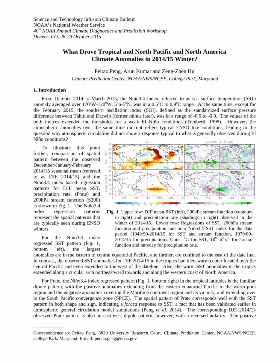
Science and Technology Infusion Climate Bulletin NOAA’s National Weather Service 40th NOAA Annual Climate Diagnostics and Prediction Workshop Denver, CO, 26-29 October 2015
______________
Correspondence to: Peitao Peng, 5830 University Research Court, Climate Prediction Center, NOAA/NWS/NCEP, College Park, Maryland; E-mail: [email protected]
What Drove Tropical and North Pacific and North America Climate Anomalies in 2014/15 Winter?
Peitao Peng, Arun Kumar and Zeng-Zhen Hu Climate Prediction Center, NOAA/NWS/NCEP, College Park, Maryland
1. Introduction
From October 2014 to March 2015, the Niño3.4 index, referred to as sea surface temperature (SST) anomaly averaged over 170oW-120oW, 5oS-5oN, was in a 0.5oC to 0.9oC range. At the same time, except for the February 2015, the southern oscillation index (SOI), defined as the standardized surface pressure difference between Tahiti and Darwin (former minus later), was in a range of -0.6 to -0.9. The values of the both indices exceeded the thresholds for a weak El Niño conditions (Trenberth 1998). However, the atmospheric anomalies over the same time did not reflect typical ENSO like conditions, leading to the question why atmospheric circulation did not show a response typical to what is generally observed during El Niño conditions?
To illustrate this point further, comparison of spatial pattern between the observed December-January-February 2014/15 seasonal mean (referred to as DJF 2014/15) and the Niño3.4 index based regression patterns for DJF mean SST, precipitation rate (Prate) and 200hPa stream function (S200) is shown in Fig. 1. The Niño3.4 index regression patterns represent the spatial patterns that are typically seen during ENSO winters.
For the Niño3.4 index regressed SST pattern (Fig. 1, bottom left), the largest anomalies are in the eastern to central equatorial Pacific, and further, are confined to the east of the date line. In contrast, the observed SST anomalies for DJF 2014/15 in the tropics had their warm center located over the central Pacific and even extended to the west of the dateline. Also, the warm SST anomalies in the tropics extended along a circular arch northeastward towards and along the western coast of North America.
For Prate, the Niño3.4 index regressed pattern (Fig. 1, bottom right) in the tropical latitudes is the familiar dipole pattern, with the positive anomalies extending from the eastern equatorial Pacific to the warm pool region and the negative anomalies covering the Maritime continent region and its vicinity, and extending over to the South Pacific convergence zone (SPCZ). The spatial pattern of Prate corresponds well with the SST pattern in both shape and sign, indicating a forced response to SST, a fact that has been validated earlier in atmospheric general circulation model simulations (Peng et al. 2014). The corresponding DJF 2014/15 observed Prate pattern is also an east-west dipole pattern, however, with a reversed polarity. The positive
Fig. 1 Upper row: DJF mean SST (left), 200hPa stream function (contours in right) and precipitation rate (shadings in right) observed in the winter of 2014/15. Lower row: Regressions of SST, 200hPa stream function and precipitation rate onto Niño3.4 SST index for the data period (1949/50-2014/15 for SST and stream function, 1979/80-2014/15 for precipitation). Units: oC for SST, 106 m2 s-1 for stream function and mm/day for precipitation rate.

SCIENCE AND TECHNOLOGY INFUSION CLIMATE BULLETIN
38
anomaly is in the western tropical Pacific and the maritime continent area, and the negative anomaly in the central equatorial Pacific. This contrast in Prate pattern between the observed and ENSO was noted by Barnston (2015).
Although the difference in Prate pattern is so striking, the observed and regression S200 patterns are surprisingly similar in the tropics. They both have an anti-cyclonic pair straddling the equator over the central Pacific. The difference between them is that the observed pattern is shifted westward about 15o with respect to the Niño3.4 index regression pattern. Furthermore, its zonal extent was narrower evolving to a cyclonic pair over the eastern Pacific. Differences in circulation pattern also occur in the extratropics. The most obvious difference is the pattern orientation over the North America. The Niño3.4 index regression pattern has a north-south dipole structure, with an anti-cyclonic anomaly in the north and a cyclonic anomaly in the south, whereas in DJF 2014/15 observations the spatial pattern has an east-west dipole structure, with cyclonic anomaly in the east and anti-cyclonic anomaly in the west. From a global perspective, in both cases the pattern over the North America is part of a wave train emanating from the tropical Pacific, and thus, the causes of the difference for both the patterns may still be in the tropics.
The role of tropical diabatic heating (as inferred from the Prate) in influencing global circulation during ENSO winters has been demonstrated in model experiments (Hoerling and Kumar 2002 and references therein) and in diagnostic analyses (Ting and Hoerling 1993, Peng 1995, DeWeaver and Nigam 2004). The anti-cyclonic (cyclonic) pair straddling the diabatic heating (cooling) in the central equatorial Pacific has been inferred to as the forced response to the heating-cooling pair over the equatorial Pacific with the Rossby wave propagation extending this response into extratropical latitudes (Gill 1980, Sardeshmukh and Hoskins 1988). The canonical ENSO heating- circulation relationship, however, does not seem to be at play for the winter of 2014/15 as the anti-cyclonic pair, instead of associated with the heating, straddles the cooling. This leads to the question as to what drove the SST and circulation anomalies, and what was the dynamics behind the tropical circulation anomalies for 2014/15 winter?
In this study we intend to examine the effects of dominant modes of wintertime SST variability using a decomposition procedure, and then assess the relative importance of these modes through a reconstruction procedure on the observed DJF 2014/15 SST and circulation anomalies.
2. Data and analysis procedures
The data used in this study include monthly mean SST, 200hPa stream function (S200) and 1000hPa wind from Jan 1949 to Feb 2015, including 66 DJF seasons, and DJF mean precipitation from 1979/80 to 2014/15 for total 36 winters. The SST is taken from Hurrell et al. (2008), the stream function from NCEP/NCAR reanalysis (Kalnay et al. 1996), and the Prate from the CPC merged analysis of precipitation (CMAP) (Xie and Akin 1996). The anomalies of these variables are with respect to the seasonal climate mean over the respective data periods. The analysis procedure begins from an empirical orthogonal function (EOF) analysis for the 66-winter Pacific SSTs. The spatial domain for the analysis is the north of 30oS and between 120oE and 80oW, including the tropical and northern part of Pacific, same as that in Hartmann
Fig. 2 Regressions of DJF mean SST (left), precipitation rate and 200hPa stream function (right) onto the first (upper), second (middle) and third (lower) principal components of the SSTs in the Pacific north of 30oS. Units are the same in Fig. 1.

PENG ET AL.
39
(2015a). The EOF calculation is based on a covariance matrix such that fewer dominant modes explain more variance. After computing the principal components (PCs), which are the time series associated with EOFs, the corresponding spatial patterns of SST are obtained with the regression of the global SSTs at each grid point onto the PCs. Following the same procedure, S200 and Prate regression patterns associated with the SST modes are also obtained. As the Prate is only available from 1979, the PC time series used for regression is from that year onward.
After the decomposition procedure, the relative importance of the SST modes in explaining the observed anomalies of the three variables for DJF 2014/15 is assessed with a reconstruction procedure. The procedure starts from the most dominant mode, and then successive modes are added at each step, until a spatial pattern resembling the observed DJF 2014/15 anomalies is reconstructed. For SST, the EOF modes can completely reconstruct the observed anomalies, because they are the modes of SST itself. For S200 and Prate, however, only a part of variance can be explained by the SST EOF modes. As a result, the constructed S200 or Prate is not as accurate as that for SST.
3. Results
Fig. 2 shows the patterns of SST, Prate and S200 associated with the first three EOF modes of SST. The corresponding PCs are displayed in Fig. 3. The first mode, explaining 41% variance of SST over the domain for the EOF analysis, is related to ENSO and referred to as ENSO mode. The SST EOF pattern and associated S200 and Prate patterns are almost identical to those from regressions with Niño 3.4 index shown in Fig. 1. The PC value of the ENSO mode for the DJF 2014/15 winter is around 1, indicating that the ENSO signal was pretty robust and was important.
The second mode, explaining about 10% variance of SST over the domain, has its major SST loading in the western and southern tropical Pacific, and also associates with anomalies in the Indian and Atlantic Oceans. The corresponding PC2 indicates that this mode is related to warming trend in the oceans, though interannual variability is also included. Its associated Prate pattern is likely a response to the SSTs with dry (wet) anomalies collocated with cold (warm) SST anomalies in the central (western) Pacific. Further, the spatial pattern of the Prate is very similar to that associated with the warm phase of ENSO, but with opposite sign and much weaker intensity. The corresponding S200 pattern in the tropics includes a cyclonic system towards the south of the negative Prate and a cross-equator system over the eastern Pacific. According to their location, shape and orientation, the former is likely forced by the diabatic cooling corresponding to the negative Prate, while the latter is more complicated. In the northern extratropics, a cyclonic system is
Fig. 3 Principle components (PCs) 1-3 of the DJF SSTs in the Pacific north of 30oS and percentages of their explained variance. PCs are normalized with their own standard deviation.

SCIENCE AND TECHNOLOGY INFUSION CLIMATE BULLETIN
40
centered over Bering Sea and with a westward extension towards Mongolia. This mode was not part of Hartmann (2015a) analysis, because their data were detrended prior to the EOF analysis.
The third mode, explaining about 8% variance of SST over the domain, is the North Pacific Mode (NPM). The SST pattern is similar to that in Hartmann (2015a), though our analysis is based on the DJF seasonal means alone, and not the monthly means over the entire annual cycle. Its larger amplitude in the extratropics may suggest a local origin, but it also has tropical loading in the western and central equatorial Pacific. The corresponding Prate pattern matches well with the SST pattern in the tropics, with positive anomaly over the warmer SST and negative anomaly over the colder SST. Though its SST anomalies are much weaker than that in the ENSO mode, the Prate anomalies are not weak, with their amplitude reaching almost a half of that for the ENSO mode. This is because that Prate is not linearly related to SST anomaly, and is much more dependent on total SST (Hoerling et al 1997). In the S200 pattern, a wave train clearly starts from the tropical western Pacific, the area of anomalous heating, and then extends across the North Pacific to North America with a ridge along the west coast and a trough over the northeastern part of the continent. The wave train then turns southeast towards the Atlantic and finally ends at the equator near western Africa. In the tropical eastern Pacific, a cyclonic pair is associated with the diabatic cooling, suggesting that it is forced by the cooling. The time series of this mode (Fig. 3c) is dominated by interannual variability before 1998, but after that by variations on a lower frequency. The PC values were notably high for DJF 2013/14 (1.75) and 14/15 (2.90), with latter being the highest in the record analyzed.
The fourth mode (not shown) is the Pacific decadal oscillation (PDO) mode, which is the second mode in Hartmann 2015a. The reason for the second mode in Hartmann 2015a to be the fourth mode here may be related to the difference in data length and trend removal or not (Wen et al. 2014). The data used in Hartmann 2015 was from 1900, about 50 years longer than here. Because its PC value for DJF 2014/15 is only 0.25, its impact is small. Other SST modes are either with small PC values for DJF 2014/15 or with weak patterns. Therefore our analysis is limited to the three leading modes.
The correlation maps corresponding to the regression maps for each mode were also checked, and it is found that most features shown in Fig. 2 are well above the 90% significant level in the T-test. We also calculated the PCs and the regression patterns with the data not including 2014/15 winter and compared them with that from the full dataset as shown in Fig. 2, and found differences to be very small.
We next reconstruct the DJF 2014/15 observed anomalies based on the EOF modes. Having examined the three leading modes and noting that SST anomaly pattern for DJF 2014/15 fits best the NPM (Fig. 2, bottom left panel), the reconstruction procedure starts from the NPM. The upper row of Fig. 4 is the reconstructed SST, Prate and S200 patterns associated with the NPM, that is, the product of PC3 value for DJF 2014/15 winter and the spatial patterns associated with the EOF3 of SST shown in Fig. 2 (bottom row). Compared to the observed anomalies shown in Fig. 1 (upper row), as expected, the reconstructed SST
Fig. 4 Reconstructed SST (left), precipitation rate and 200hPa stream function (right) for DJF 2014/15 with spatial patterns shown in Fig. 2 and PCs shown in Fig. 3. Upper row is for using NPM alone, middle row for using both NPM and ENSO mode, and lower row for using all NPM, ENSO and warming trend modes. Unites are the same as that in Fig. 1.

PENG ET AL.
41
resembles the observation very well, particularly for the warm anomalies over the Pacific domain. However some differences are also obvious. The strong cold anomaly in the eastern equatorial Pacific is not found in the DJF 2014/15 observation, and the intensity of the reconstructed warm SST anomaly is too weak. For the Prate, the reconstructed pattern matches well the observed anomaly not only in the tropics, but also in North Pacific and North America. A major difference is in the intensity in the tropical Pacific, where the reconstructed anomaly is much stronger than the observed. For the S200, as described before, the reconstructed pattern is a wave train emanating from the diabatic heating area (correspond to the Prate) in the tropical western Pacific, with its features matching well with the observations, particularly over the North America. Major differences are that the anti-cyclonic center in the tropical central Pacific is shifted westward, and the intensity of the wave train appears weaker. Therefore, the NPM, although prominent, it alone is not adequate to explain the observed DJF 2014/15 anomalies in the tropical and North Pacific.
Because the amplitude of the ENSO mode is the strongest among all (Fig. 1) and PC1 value for DJF 2014/15 is around 1.0 for this winter, the contribution of the ENSO mode needs to be considered. The middle row of the Fig. 4 presents the reconstructed patterns after adding the ENSO mode. Comparing them with the reconstruction with the NPM alone (Fig. 4, upper row) and that from the observations (Fig. 1, upper row), we can see that the correspondence with the observed anomalies improved: (a) the cold SST anomaly in the eastern equatorial Pacific disappeared and the intensity of the warm SST anomalies increased to the level in observations; (b) the intensity of tropical Prate also reduced to the level in the observation; (c) the westward shift of the anti-cyclonic center also corrected to some extent; (d) the wave amplitude increased to that in the observation. Improvements, however, were not unanimous, for example, the trough over the northeastern part of North America became weaker, and so is the cyclonic pair in the tropical eastern Pacific.
The results of the reconstruction by adding the mode 3 are displayed in the lower row of Fig. 4. As already indicated by the mode’s small PC value of 0.5 and the relatively weak circulation and precipitation patterns, the improvement is quite limited. A discernible improvement for SST is in the tropical western Pacific and India Ocean, where the SSTs became a bit warmer. Overall, the SST, precipitation and circulation anomalies in the winter of 2014/15 basically can be explained by the NPM and ENSO mode. The NPM was a dominant factor, which explains why the atmospheric anomalies did not conform to the typical ENSO response pattern (Barnston 2015).
4. Summary and discussion
In an effort to explain why the atmospheric circulation and SST anomalies of 2014/15 winter in the central equatorial Pacific lacked ocean-atmosphere coupling seen in a typical ENSO event, this study decomposed the SST, precipitation rate and 200hPa stream function anomalies for the DJF 2014/15 into the patterns related to the principal components of the DJF SST variability. We then identified the relative importance of these patterns in contributing to observed DJF 2014/15anomalies. It is found that the anomalies of the three variables were determined by the patterns related to the two SST modes, the NPM and the ENSO mode. The contribution from the NPM dominated and resulted in the seemingly uncoupled air-sea relationship in the central equatorial Pacific and the east-west structure of the observed circulation anomalies over the North America. The contribution of the ENSO mode was important for the observed SST anomalies in the eastern equatorial Pacific and for the circulation in the central equatorial Pacific. The ENSO mode was also important for the intensity of SST, precipitation rate and circulation patterns to reach the levels in the observation. The impact from the warming trend mode was found to be much small.
Acknowledgments. We would like to thank Dr. Caihong Wen for her constructive suggestions.
References
Ashok, K., S. K. Behera, S. A. Rao, H. Weng, and T. Yamagata, 2007: El Niño Modoki and its possible teleconnection. J. Geophys. Res., 112, C11007.
Barnston, T., 2015: Do recent global precipitation anomalies resemble those of El Niño? http://www.climate.gov/news-features/blogs/enso.

SCIENCE AND TECHNOLOGY INFUSION CLIMATE BULLETIN
42
Bjerknes, J., 1969: Atmospheric teleconnections from the equatorial Pacific. Mon. Wea. Rev., 97, 163– 172.
DeWeaver, E., and S. Nigam, 2004: On the forcing of ENSO teleconnections by anomalous heating and cooling. J. Climate, 17, 3225–3235.
Gill, A.E., 1980: Some simple solutions for heat-induced tropical circulation. Q. J. R. Meteorol. Soc., 106, 447–462.
Hartmann, D., 2015a: Pacific sea surface temperature and the winter of 2014, Geophys. Res. Lett., 42, doi:10.1002/2015GL063083.
Hartmann, D., 2015b: The tropics as a prime suspect behind the warm-cold split over North America during recent winters, http://www.climate.gov/news-features/blogs/enso.
Hoerling, M., A. Kumar, and M. Zhong, 1997: El Niño, La Niña, and the nonlinearity of their teleconnections. J. Climate, 10, 1769–1786.
Hoerling, M., and A. Kumar, 2002: Atmospheric response patterns associated with tropical forcing. J. Climate, 15, 2184–2203.
Hurrell, J., J. Hack, D. Shea, J. Caron, and J. Rosinski, 2008: A new sea surface temperature and sea ice boundary dataset for the community atmosphere model. J. Climate, 21, 5145–5153.
Kao, H.-Y., and J.-Y. Yu, 2009: Contrasting Eastern-Pacific and Central-Pacific types of ENSO. J. Climate, 22, 615–632.
Kalnay, E. and coauthors, 1996: The NCEP/NCAR 40-year reanalysis project. Bull. Amer. Meteor. Soc., 77, 437-471.
Peng, P., 1995: Dynamics of stationary wave anomalies associated with ENSO in the COLA GCM. Ph.D. thesis, University of Maryland, College Park, 180 pp.
Peng, P., A. Kumar, and B. Jha, 2014: Climate mean, variability and dominant patterns of the Northern Hemisphere wintertime mean atmospheric circulation in the NCEP CFSv2, Climate Dynamics, 42, 2783-2799.
Sardeshmukh, P. and B. Hoskins, 1988: The generation of global rotational flow by steady idealized tropical divergence. J. Atmos. Sci., 45, 1228–1251.
Saha, S. and coauthors, 2014: The NCEP Climate Forecast System Version 2. J. Climate, 27, 2185–2208.
Ting, M. and M. Hoerling, 1993: Dynamics of stationary wave anomalies during the 1986/87 El Niño. Climate Dynamics, 9, 147-164.
Wen, C., A. Kumar, and Y. Xue, 2014: Factors contributing to uncertainty in Pacific Decadal Oscillation index, Geophys. Res. Lett., 41, 7980–7986, doi:10.1002/2014GL061992.
Xie, P., and P. A. Akin, 1996: Analysis of global monthly precipitation using gauge observations, satellite estimates, and Numerical model predictions. J. Climate, 9, 840-858.

Science and Technology Infusion Climate Bulletin NOAA’s National Weather Service 40th NOAA Annual Climate Diagnostics and Prediction Workshop Denver, CO, 26-29 October 2015
______________ *Correspondence to: Panmao Zhai, State Key Laboratory of Severe Weather, Chinese Academy of Meteorological Sciences, 46 Zhong-guan-cun-nan-da-jie, Haidian, Beijing 100081, China; E-mail: [email protected].
Teleconnection Patterns Impacting on the Summer Consecutive Extreme Rainfall in Central-Eastern China
Junmei Lü1,2, Yun Li2, Panmao Zhai1*, Junming Chen1, and Tongtiegang Zhao2 1Chinese Academy of Meteorological Sciences, Beijing, China
2CSIRO Mathematics, Informatics and Statistics, Wembley, Western Australia, Australia
1. Introduction
Extreme weather and climate events such as deadly heat waves, devastating floods and severe droughts can damage human societies and ecosystems. Numerous previous studies have demonstrated that there has been an increase in the frequency and intensity of extreme weather events in recent decades (Meehl et al. 2000; Zhai et al. 2005; Fischer et al. 2007; Kyselý 2008). For instance, heat waves have become longer and hotter, and heavy rains and flooding have become more intense and more frequent. Consecutive extreme rainfall (CER) events, which usually cause large-scale floods, mudflows and landslides, are defined as “consecutive rainfall persisting for at least 3 days with the daily rainfall exceeding 50 mm” (Chen and Zhai 2013). Chen and Zhai (2013) proposed that individual-station-based CER events occurred mainly in Central-Eastern and South China, which are the most populated and economically developed regions in China.
Recent studies have shown that the large-scale systems that produce CER are often related to anomalous and persistent atmospheric wave patterns such as blocking anticyclones and cutoff lows, which are characterized by slow moving or stagnant features and related to teleconnection patterns (Zhou et al. 2009; Lau and Kim 2012;Chen and Zhai 2014). The goal of this study is to investigate the dominant modes of the CER over Central-Eastern China and to identify their corresponding persistent circulation patterns. The impacts of anomalous SSTs and Rossby wave propagation on the formation of teleconnection patterns are also discussed.
2. Methodology
The 95th percentile is widely used to evaluate the threshold for extreme rainfall. Chen and Zhai (2013) calculated the 95th percentile of daily total precipitation in China during the warm season and found that a daily precipitation amount of 50 mm exceeded the 95th percentile at over 90% of stations. Hence, the absolute threshold of extreme rainfall is defined as exceeding 50 mm for daily total precipitation. The CER events over Central-Eastern China are defined according to the following criteria: (1) the JJA daily rainfall exceeds 50 mm at one or more weather stations, (2) the extreme rainfall persists for at least 3 consecutive days, and (3) the CER events end when daily rainfall is less than 50 mm d-1 over 2 consecutive days. This definition ensures the regional occurrences of CER events.
The CER event definition was applied to a 32-year period (1979-2010) for 210 weather stations. This analysis resulted in 86 CER events and 340 event days. Empirical orthogonal function (EOF) analysis was performed on 230 event days to assess the dominant modes of the CER (EOFs) and their corresponding time series (PCs). The relationship between various circulation patterns and the CER modes was determined by correlating grid-point anomalies of an atmospheric field onto an index, for example, the PC of an EOF, or the SST index. To find out the mechanisms that maintain the teleconnection wave trains associated with CER events, we analyzed the wave-activity flux formulated by Takaya and Nakamura (2001) and the ray paths derived by Hoskins and Karoly (1981). Ray equations for stationary waves were given by Wang et al. (2007).
3. Analysis
An EOF analysis of the CER revealed three dominant modes that together account for 44% of the total CER variance (Fig. 1 left panels). The first mode represents the consistent changes in the CER events over the

SCIENCE AND TECHNOLOGY INFUSION CLIMATE BULLETIN
44
entire region (Fig. 1a). This mode suggests a climate status that is related to the occurrence of CER events over the entire area. The second mode has a dipolar structure with inverse variations of the CER in the southern Yangtze River (SYR) and the Yangtze-Huaihe River Valley (YHRV) (Fig. 1d). The third mode is characterized by a tripolar structure (Fig. 1g). To compare the dominant modes of the CER versus non-extreme rainfall (non-ER, <50 mm d-1), the three leading EOFs of non-ER are also shown in Fig. 1 (right panels). The three leading EOFs of non-ER explain just 25% of the total non-ER variance, which is much less than 44% for the CER. Although the first mode of non-ER (Fig. 1c) has a uniform regional variation similar to the first mode for the CER, the spatial correlation between the two EOF1 patterns is -0.16, suggesting that the two types of rainfall have totally different distributions. For example, the highest rainfall value is located in the center of the area for the CER (Fig. 1a), while the highest values for the non-ER are located in the northwestern and southeastern corners (Fig. 1c). The second mode of non-ER has a dipolar structure (Fig. 1f) and significantly correlates with the second mode of the CER (r=0.55). The third mode of non-ER (Fig. 1i) does not share the tripolar structure of the EOF3 for the CER, although there is a significant correlation between the two EOFs (r=0.31). These differences demonstrate the importance of rainfall type classification according to rainfall intensity.
To derive teleconnection pattern associated with the first mode of the CER, one-point correlation is performed on 500 hPa geopotential height anomalies at days -6, -4, -2 and 0 with reference to the base point denoted by the box [28°- 43° N, 130°- 160° W] in Fig. 2 a-b, and another box [20°- 35° N, 130°- 160° W] in
Fig. 1 The EOF modes of the CER (left panels), PCs of the CER (middle panels), and EOF modes of non-ER rainfall (right panels) during JJA. The explained variance of each EOF is indicated at the top. Closed circles in (a) show the locations of the 210 observation stations in Central-Eastern China.

LÜ ET AL.
45
Fig. 2 c-d. A barotropic circumglobal teleconnection (CGT) pattern with a zonal wavenumber-3 structure occurs from days -6 to 0. Pressure variations over northeastern North America, the North Atlantic, and the Caspian Sea are all in phase with variation over the subtropical North Pacific (SNP), as shown by significant positive correlations. In contrast, pressure fluctuations over North America, northwestern Europe, and the Lake Baikal-East Asia area exhibit significant negative correlations. Ding and Wang (2005) also found that a CGT pattern with a zonal wavenumber-5 structure exists during boreal summer. This CGT influences rainfall and temperature in continental regions including East Asia.
The second mode of the CER shows inverse variations in the SYR and the YHRV. Fig. 3 displays the one-point correlation between the base point (15°- 25° N, 90°- 130° E) and 500 hPa geopotential height anomalies at lags of 0, -5, -10, and -15 days. It is apparent that a negative Pacific-Japan (PJ) teleconnection pattern occurs 15 days prior to the CER events and maintains this wave train thereafter.
The third mode of the CER events indicates that the probability of CER occurring in the YRV is low, while it is high in the Huaihe River Valley (HRV) and the SYR. As shown in Fig. 4, a negative Eurasian pattern (EU) exists at lags of -6, -4, -2 and 0 days. Significant negative correlations are located in the northeastern Atlantic and the area east of the Caspian Sea to Lake Baikal. On the other hand, significant positive correlations exist over the Mediterranean Sea to Western Europe and East Asia. It should be noted that the positive correlation over the East Asia is related to the Bonin high, suggesting that the negative EU-like teleconnection plays an important role on the formation of the Bonin high.
Fig. 2 One-point correlation map between the base point (box) and 500 hPa geopotential height anomalies at day 0 (a), day -2 (b), day -4 (c), and day -6 (d). Shaded areas denote significance at the 0.10, 0.05 and 0.01 levels.
Fig. 3 One-point correlation map between the base point (box) and 500 hPa geopotential height anomalies for day 0 (a), day -5 (b), day -10 (c), and day -15 (d). Shaded areas indicate significance at the 0.10, 0.05 and 0.01 levels.

SCIENCE AND TECHNOLOGY INFUSION CLIMATE BULLETIN
46
4. Concluding remarks
In this study, CER events over Central-Eastern China during the period from 1979-2010 were identified based on the new definition. The dominant modes of the CER were determined based on EOF analysis. Our results show that the spatial distribution of the CER can be attributed to certain persistent circulation patterns, which makes sense because prolonged weather conditions can enhance the possibility of extreme events. When CER events occur over the entire region, the Western Pacific Subtropical High (WPSH) prevails in South China and the northern South China Sea (SCS); 5 days prior to CER event onset, the WPSH is located in the middle of the SCS, after which it migrates northward, bringing water vapor from the western North Pacific (WNP) to the SYR and then the YHRV. Additionally, a barotropic CGT pattern with two major components, namely the Lake Baikal trough and the Ural blocking high, is found in geopotential height and persists from days -6 to 0. On the other hand, a negative PJ pattern is identified in geopotential height 15 days before the CER events occur over the YHRV. The WPSH, blocking high around the Sea of Okhotsk, and the anomalous low pressure south of Lake Baikal are three components of the negative PJ pattern. Furthermore, double blocking highs appear around the Ural mountains and the Sea of Okhotsk, distinguishing the persistent circulations of the second CER mode from the first mode. Moisture convergence and ascending motion anomalies prevail over the YHRV 5 days prior to CER event onset, accompanying the northwestward extension of the WPSH from the WNP to South China and the SYR. The third mode is associated with a negative EU-like teleconnection that appears 6 days before CER event onset. As one component of the EU-like teleconnection, the Bonin high covers East Asia from days -5 to 0 with moisture convergence and ascending motion anomalies over the HRV and SYR. This configuration of circulation anomalies favors the occurrence of CER events over the HRV and SYR. Thus, the configuration of persistent circulation anomalies is responsible for the CER distributions.
Rossby wave propagation plays a key role in the formation and persistence of teleconnection patterns. Note that the three teleconnection patterns associated with the three CER modes are induced by SST anomalies around their base points. The ray paths based on these three base points correspond to the CGT, PJ and EU wave trains, suggesting the importance of propagating Rossby waves for the formation of teleconnection patterns, although the mechanism through which stationary Rossby waves respond to these heat sources needs to be investigated further.
References
Chen Y., and P. M. Zhai, 2013: Persistent extreme precipitation events in China during 1951-2010. Clim. Res., 57, 143–155, doi: 10.3354/cr01171.
Chen Y., and P. M. Zhai, 2014: Precursor circulation features for persistent extreme precipitation in Central-Eastern China. Wea. Forecasting, 29, 226–240, doi: 10.1175/ WAF-D-13-00065.1.
Fig. 4 One-point correlation map between the base point (box) and 500 hPa geopotential height anomalies for day 0 (a), day -2 (b), day -4 (c), and day -6 (d). Shaded areas indicate significance at the 0.10, 0.05 and 0.01 levels.
LÜ ET AL.
47
Ding, Q. H., and B. Wang, 2005: Circumglobal teleconnection in the Northern Hemisphere summer. J. Climate, 18, 3483–3505, doi: 10.1175/JCLI3473.1.
Fischer, E. M., Seneviratne S. I., Lüthi D., and Schär C., 2007: Contribution of land- atmosphere coupling to recent European summer heat waves. Geophys. Res. Lett., 34, L06707, doi: 10.1029/2006GL029068.
Hoskins, B. J., and Karoly, D. J., 1981: The steady linear response of a spherical atmosphere to thermal and orographic forcing. J. Atmos. Sci., 38: 1179–1196, doi: 10. 1175/1520-0469(1980)038<1179.TSLROA>2.0.CO:2
Kyselý, J. 2008: Influence of the persistence of circulation patterns on warm and cold temperature anomalies in Europe: Analysis over the 20th century. Global and Planetary Change, 62, 147–163, doi: 10.1016/j.gloplacha.2008.01.003.
Lau, W. K. M., and K.-M. Kim, 2012: The 2010 Pakistan flood and Russian heat wave: teleconnection of hydrometeorological extremes. J. Hydrometeor., 13: 392– 403, doi: 10.1175/JHM-D-11-016.1.
Meehl, Gerald A., and Coauthors, 2000: An introduction to trends in extreme weather and climate events: observations, socioeconomic impacts, terrestrial ecological impacts, and model projections. Bull. Amer. Meteor. Soc., 81, 413–416, doi: 10.1175/1520- 0477(2000)081<413.TSLROA>2.0.CO:2.
Takaya, K., and H. Nakamura, 2001: A formulation of a phase-independent wave-activity flux for stationary and migratory quasigeostrophic eddies on a zonally varying basic flow. J. Atmos. Sci., 58, 608–627, doi: 10.1175/1520-0469 (2001)058<0608: AFOAPI>2.0.CO;2.
Wang Y., K. Yamazaki, and Y. Fujiyoshi, 2007: The interaction between two separate propagations of Rossby waves. Mon. Wea. Rev., 135, 3521–3540, doi: 10.1175/MWR3486.1.
Zhai, P. M., X. B. Zhang, H. Wan, and X. H. Pan, 2005: Trends in total precipitation and frequency of daily precipitation extremes over China. J. Climate, 18, 1096–1108, doi: 10.1175/JCLI-3318.1.
Zhou, W., J.C. L. Chan, W. Chen, J. Ling, J. G. Pinto, and Y. P. Shao. 2009: Synoptic-scale controls of persistent low temperature and icy weather over southern China in January 2008. Mon. Wea. Rev., 137: 3978–3991, doi: 10.1175/2009MWR 2952.1.
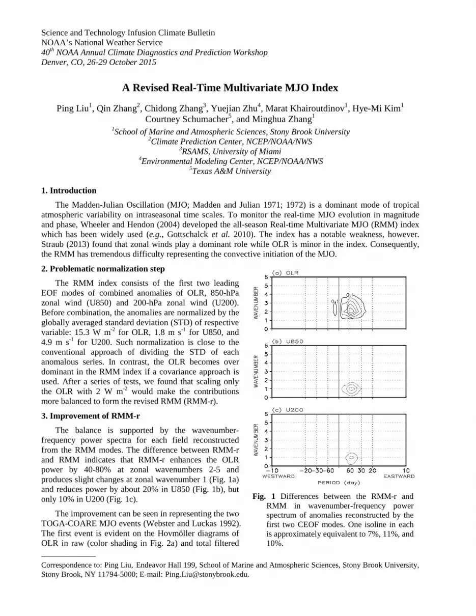
Science and Technology Infusion Climate Bulletin NOAA’s National Weather Service 40th NOAA Annual Climate Diagnostics and Prediction Workshop Denver, CO, 26-29 October 2015
______________
Correspondence to: Ping Liu, Endeavor Hall 199, School of Marine and Atmospheric Sciences, Stony Brook University, Stony Brook, NY 11794-5000; E-mail: [email protected].
A Revised Real-Time Multivariate MJO Index
Ping Liu1, Qin Zhang2, Chidong Zhang3, Yuejian Zhu4, Marat Khairoutdinov1, Hye-Mi Kim1 Courtney Schumacher5, and Minghua Zhang1
1School of Marine and Atmospheric Sciences, Stony Brook University 2Climate Prediction Center, NCEP/NOAA/NWS
3RSAMS, University of Miami 4Environmental Modeling Center, NCEP/NOAA/NWS
5Texas A&M University
1. Introduction
The Madden-Julian Oscillation (MJO; Madden and Julian 1971; 1972) is a dominant mode of tropical atmospheric variability on intraseasonal time scales. To monitor the real-time MJO evolution in magnitude and phase, Wheeler and Hendon (2004) developed the all-season Real-time Multivariate MJO (RMM) index which has been widely used (e.g., Gottschalck et al. 2010). The index has a notable weakness, however. Straub (2013) found that zonal winds play a dominant role while OLR is minor in the index. Consequently, the RMM has tremendous difficulty representing the convective initiation of the MJO.
2. Problematic normalization step
The RMM index consists of the first two leading EOF modes of combined anomalies of OLR, 850-hPa zonal wind (U850) and 200-hPa zonal wind (U200). Before combination, the anomalies are normalized by the globally averaged standard deviation (STD) of respective variable: 15.3 W m-2 for OLR, 1.8 m s-1 for U850, and 4.9 m s-1 for U200. Such normalization is close to the conventional approach of dividing the STD of each anomalous series. In contrast, the OLR becomes over dominant in the RMM index if a covariance approach is used. After a series of tests, we found that scaling only the OLR with 2 W m-2 would make the contributions more balanced to form the revised RMM (RMM-r).
3. Improvement of RMM-r
The balance is supported by the wavenumber-frequency power spectra for each field reconstructed from the RMM modes. The difference between RMM-r and RMM indicates that RMM-r enhances the OLR power by 40-80% at zonal wavenumbers 2-5 and produces slight changes at zonal wavenumber 1 (Fig. 1a) and reduces power by about 20% in U850 (Fig. 1b), but only 10% in U200 (Fig. 1c).
The improvement can be seen in representing the two TOGA-COARE MJO events (Webster and Luckas 1992). The first event is evident on the Hovmöller diagrams of OLR in raw (color shading in Fig. 2a) and total filtered
Fig. 1 Differences between the RMM-r and RMM in wavenumber-frequency power spectrum of anomalies reconstructed by the first two CEOF modes. One isoline in each is approximately equivalent to 7%, 11%, and 10%.

LIU ET AL.
49
MJO (contours in Figs. 2a, 2c, and 2d). It started near the end of November 1992 in the Western Indian Ocean. A large dry patch was then embedded in the evolution for about 10 days between 6 and 16 December, causing the wet band to be very narrow. This patch disappeared in the filtered MJO. After this patch, a wet phase redeveloped in the Western Pacific and peaked at about 170◦E with a magnitude of -50 ~ -70 W m-2 in raw OLR while the corresponding value was less than half in the filtered MJO (only two contours). The second event was initiated over Africa and followed immediately the first event. It had two peak phases in raw OLR: one in the Central Indian Ocean with a magnitude smaller than -60 W m-2, and the other near the dateline of about -60 W m-2.
The amplitudes in RMM and RMM-r overall capture both events from their initiation to peak phases (Fig. 2b), while notable changes were made by RMM-r during the first event. The RMM-r amplitude becomes above 1 again on 18 December, which is about one week earlier than RMM. Between 16 and 25 December, the RMM-r amplitude is nearly twice much as RMM, more consistent with the evolution and magnitude of the peak around 21 December on the Hovmöller diagram (cf. Fig. 2a). For the second MJO event, RMM-r has two peaks on 5 and 15 January 1993 and they are about 20-40% larger than the RMM peaks, which is more consistent with the Hovmöller diagram as well.
The reconstructed OLR amplitudes are improved as on Hovmöller diagrams (Figs. 2c and 2d). For the first event, RMM-r (Fig. 2d) has a much larger magnitude than RMM (Fig. 2c), and the duration of the suppressed phase before the redevelopment is much shorter. For the second event, the reconstructed OLR between 110°E and the date line is about 10-20 W m-2 smaller in RMM-r (Fig. 2d) than in RMM (Fig. 2c), suggesting stronger convection in RMM-r and closer to the raw and filtered MJO in Fig. 2a.
The improvement can be demonstrated on the RMM phase diagram too. For the first TOGA-CORE event (Fig. 3a), RMM-r (blue curve) detects it starting over the Western Indian Ocean in Phase 2, which is more eastward than RMM (black curve) in Phase 1 as shown by the different locations of the two black dots. The RMM-r remains outside of the unit circle for a few days and enters the circle at the Central Indian Ocean, also more eastward and with larger amplitude than the RMM. Later, the RMM-r emerges out of the circle in Phase 5 slightly to the east of the Maritime Continent and remains strong for several days towards the end in Phase 6 corresponding to the MJO redevelopment (cf. Fig. 2a). This phase evolution of RMM-r is also in a better agreement with the raw OLR than that
Fig. 2 The two TOGA-CORE MJO events for (a) raw OLR anomaly (shading) and filtered MJO (contour with interal 10 W m-2 and 0 being omitted); (b) amplitudes of RMM (black) and RMM-r (blue); (c) reconstructed anomalies (shading with uneven intervals) by RMM and total filtered MJO (contour as in a); and (d) same as (c) but by RMM-r.
Fig. 3 Catesian phase diagrams of RMM (black) and RMM-r (blue) for the two events during TOGA-CORE (a) 28 November 1992 - 5 January 1993 and (b) 1 January - 15 Febrary 1993.

SCIENCE AND TECHNOLOGY INFUSION CLIMATE BULLETIN
50
of RMM. The enhanced OLR variance in RMM-r obviously contributes to the change (cf. Fig. 2). For the second event during TOGA-CORE, both RMM and RMM-r represent its evolution well (Fig. 3b). There are still a couple of notable changes in the RMM-r. It peaks in Phases 3 over the Eastern Indian Ocean and Phase 4 over the Maritime Continent, while RMM peaks only once over the central Indian Ocean. The RMM-r amplitude is larger than RMM in Phases 1-5. Clearly RMM-r is more consistent with the actual MJO evolution.
This work has been published in Monthly Weather Review in 2016.
References
Gottschalck, J. and Coauthors, 2010: A framework for assessing operational Madden-Julian Oscillation forecasts: A CLIVAR MJO Working Group Project. Bull. Amer. Meteor. Soc., 91, 1247-1258.
Liu, P., Q. Zhang, C. Zhang, Y. Zhu, M. Khairoutdinov, H.-M. Kim, C. Schumacher, and M. Zhang, 2016: A revised real-time multivariate MJO index. Mon. Wea. Rev., 144, 627–642. doi: http://dx.doi.org/10.1175/MWR-D-15-0237.1
Madden, R. A., and P. R. Julian, 1971: Detection of a 40-50 day oscillation in the zonal wind in the tropical Pacific. J. Atmos. Sci., 28, 702-708.
Madden, R. A., and P. R. Julian, 1972: Description of global-scale circulation cells in the tropics with a 40-50 day period. J. Atmos. Sci., 29, 1109-1123.
Straub, K. H., 2013: MJO initiation in the Real-time Multivariate MJO index. J. Climate, 26, 1130-1151.
Webster, P. J., and R. Lukas, 1992: TOGA COARE: the coupled ocean-atmosphere response experiment. Bull. Amer. Meteor. Soc.,73, 1377-1416.
Wheeler, M. C., and H. H. Hendon, 2004: An all-season Real-time Multivariate MJO index: Development of an index for monitoring and prediction. Mon. Wea. Rev., 132, 1917-1932.

Science and Technology Infusion Climate Bulletin NOAA’s National Weather Service 40th NOAA Annual Climate Diagnostics and Prediction Workshop Denver, CO, 26-29 October 2015
______________
Correspondence to: Joseph S. Renken, KOPN Radio, Columbia MO; E-mail: [email protected].
Using the Bering Sea and Typhoon Rules to Generate Long-Range Forecasts II: Case Studies
Joseph S. Renken1, Joshua Herman2, Daniel Parker3, Travis Bradshaw4, and Anthony R. Lupo5 1KOPN Radio, Columbia MO
2University of Wisconsin – Fox Valley 3Western Illinois University, Macomb, IL
4Moberly Area Community College, Columbia, MO 5Department of Soil, Environmental, and Atmospheric Science, University of Missouri, Columbia, MO
1. Introduction
Dynamic weather forecasting using numerical models can be done reliably out to approximately seven days, and has an absolute limit of about 10-14 days. Beyond this point, statistical forecasts are typically made. These limitations are due to the characteristics of the earth and atmosphere, but also the lack of data, knowledge of the physical processes, and measurement error (e.g., Haltiner and Williams 1980; Durran 1999). Error in the initial and/or boundary conditions can render model forecasts as quickly as a few days (e.g., Lorenz 1965), or alternatively two forecasts with slight difference in the initial conditions could evolve in radically different ways over the course of time. This problem is referred to as sensitivity to the initial conditions. One way to mitigate or qualitatively evaluate this problem is ensemble forecasting, a forecasting product that has been available for more than two decades (e.g., Toth and Kalnay 1993, 1997; Tracton and Kalnay 1993).
Forecasting beyond two weeks could also use ensemble forecasting methods, and the Climate Prediction Center (CPC) has developed an experimental product that makes probabilistic forecasts in the three to four week time period1. This particular time period has not been forecast for traditionally, as there are monthly and seasonal forecasts made by the Climate Prediction Center. Renken et al. (2015) demonstrated the success of temperature predictions in the 6-30 day period for the United States using the Bering Sea Rule (BSR) and/or Typhoon Rule (TR), which showed success over climatology. This skill was especially measurable in forecasting events that were two or more standard deviations above or below climatology. The BSR and TR are based on Pacific and North American (PNA) region teleconnectivity, which was defined statistically by Wallace and Gutzler (1981). Renken et al. (2015) further showed that Pacific Region blocking has a strong correlation to weather and climate in the middle part of the USA, via the strong impact on the teleconnection patterns within the PNA region.
The motivation for this work is to demonstrate further the utility of the BSR and TR for prediction in the two-to-four week period. Case studies will be presented in order to demonstrate the capabilities of these indexes. We will also demonstrate that there is a strong degree of autocorrelation in this time frame by examining the PNA index.
2. Data and methodology
a. data
The data used for this work are the National Centers for Environmental Prediction / National Center for Atmospheric Research (NCEP/NCAR) re-analyses which are archived in Boulder, CO2. These data were the 500 hPa height fields on the 2.5o x 2.5o latitude/longitude grid daily from 1948 - present. The daily PNA
1 http://www.cpc.ncep.noaa.gov/products/predictions/WK34/ 2 http://www.esrl.noaa.gov/psd/data/reanalysis/reanalysis.shtml

SCIENCE AND TECHNOLOGY INFUSION CLIMATE BULLETIN
52
index information was also available from CPC which used the NCEP/NCAR re-analyses and are available from 1 January 1950 - present, which represents a 66 year period as of 31 December, 2015.
b. Methods and definitions
In order to determine if there was predictability in the PNA index time series, autocorrelation was performed by lagging the PNA index from 1 January 2012 to 31 December 2013. Autocorrelation can be used in order to test for chaotic or cyclical behavior in a data set. If a system has limited predictability, then the correlation will fall to zero with further lag and remain there. If there is cyclical behavior, correlation will increase near the time-scale of the forcing function. Additionally, the entire time series was decomposed using Fourier series in order to isolate significant power in the time series.
The BSR correlates 500 hPa heights in the Bering Sea Region to three points in the USA which show strong correlation. These three points are in southern Utah, western MO, and near Long Island, using a similar methodology to Wallace and Gutzler (1981). The primary correlation time is in the two to three week time-frame. The TR correlates 500 hPa heights in East Asia to points in the USA, and the primary time-scale in one–to-two weeks.
3. Periodicity in the 500 hPa height field
The results of testing the PNA index derived from the 500 hPa height field using autocorrelation for the two year period of 2012-2013 are shown in Fig 1. The time series was auto-regressed from 1 to 130 days. The correlation falls rapidly, but then increases slightly around 20 and 34 days. There is a strong non-zero peak also found in the 50-55 day period. While this hints at predictability in the three-to-four week time frame and beyond, this test by itself cannot identify recurrence in the desired time frame. Additionally, this period is a small segment of the climatological record for the PNA region. Tests on other parts of the 66 year series reveal similar behavior to that shown in Fig. 1.
Next, the time series of the daily PNA index for the 66 year period were decomposed using Fourier series decomposition (Fig. 2). The entire decomposition is not shown in order to focus on the time period in question. The decomposition shows spectral peaks at several wave numbers, and the period can be determined by dividing the wave number by the spectral peak. For example, in addition to those peaks associated with the annual cycle there were strong peaks around wave numbers 505, 570, and 610, corresponding to a period of about 47, 42, and 39 days (not shown). These peaks probably correspond to a long-period Rossby Wave. This analysis cannot determine if these are different peaks forced by different processes, or more likely, the same
Fig. 1 The autocorrelation of the PNA index from 1 January 2012 to 31 December 2013.
Fig. 2 The spectral decomposition of the 66-year time series of the PNA index. The abscissa is wave number 1000 to 1500, and the ordinate is spectral power.

RENKEN ET AL.
53
peak whose period may be modulated by annual cycle, El Nino and Southern Oscillation (ENSO), the Pacific Decadal Oscillation (PDO), or climate change. The latter seemed to be the case when testing different parts of the 66 year time series using auto correlation. Further analysis would be needed to verify this assertion.
The time period of interest is shown is Fig, 2, which shows the spectral peaks from wave number 1000 to 1500, and these correspond to periods of 23 to 16 days. There are peaks found near 1000-1010 and in the 1140-1190 range, which correspond to 24 and 21 days respectively. This analysis, combined with the autocorrelation, hint at predictability in the two - three week time scale, which is similar to the result obtained from autocorrelation.
4. Two case studies
a. 28 April 2014 severe weather
On 28 April, 2014, severe weather occurred across the middle southeast USA, and the St. Louis region. The Storm Prediction Center (SPC) archived several reports of tornadoes, large hail, and strong winds (Fig 3d), and this was associated with a strong trough at 500 hPa located over the plains states (Fig 3c), and this was associated with a well-developed low pressure at the surface. Examining the Bering Sea region about 20 days prior (8 April, 2014) shows a strong 500 hPa low near the Kamchatka Peninsula and the Aleutians (Fig 3a). A figure showing the Bering Sea region on 28 April would show a trough in the same area as in Fig. 3a. Thus there is an approximately two to four week cycle in the PNA index as shown in Section 3. About eight days before the 28 April event, a strong low was located over East Asia (Fig. 3b) which corresponds to the TR.
Fig. 3 The 500 hPa height anomalies versus the 1981-2010 climatology over the Bering Sea region for a) 8 April 2014, b) 20 April 2014, and c) over the Continental USA for 28 April 2014. d) The Continental USA severe weather reports.
(a)
(b)
(c)
(d)

SCIENCE AND TECHNOLOGY INFUSION CLIMATE BULLETIN
54
Also, low pressure would exist in the Bering Sea region again on 28 April (not shown).
b. Typhoon Nuri, November 2014
The case of Typhoon Nuri was cited briefly by Renken et al. (2015) as a successful example of the BSR and TR. In early November, 2014, Typhoon Nuri moved poleward in the western Pacific becoming extratropical and deepening to 924 hPa as the strongest North Pacific cyclone ever. This was reflected in the 500 hPa height field as a strong low over the western Bering Sea (Fig. 4a) during the 8-10 November 2014 period. This cyclone was upstream of a weak blocking event, which had onset at 1200 UTC 5 November at about 170o W (see http://weather.missouri.edu/gcc/blocknh.pdf). The cyclone interacted with the blocking event, strengthening the block through the same mechanism shown in Lupo and Smith (1995), Lupo (1997), or Lupo and Bosart (1999). This blocking event induced persistent troughing over North America, which was particularly strong in the middle of and late in the month (Fig. 4c). In this case the, the PNA pattern intensified strongly during the strengthening of the surface cyclone and blocking event. During late November there was also an upstream trough in the Bering Sea region. In the middle of November troughing correlating with the TR was present over East Asia (Fig 4b). There was also strong indication of the mid-November cold event in association with the remnants of Nuri using the TR (Fig. 4a).
5. Discussion, summary, and conclusions
This work furthers the study presented last year which showed that there was skill above climatology in using the BSR or TR for making long-range forecasts in the one to four week time frame, especially for extreme events. The BSR and TR simply use two of the action centers from the PNA index looking at the two positively correlated centers generally (the Bering Sea and the Eastern USA primarily). In this study, the PNA index is used as a surrogate for the 500 hPa height field in the region. Autocorrelation of the PNA time series for 2012-2013 showed cyclical behavior in the correlation series (lagged by up to 130 days), and similar behavior was shown in other parts of the time series. This test suggested that there may be predictability in the 20 and 34 day time period, as well as a strong increase in the correlation peaking at 50-55 days. In our study, the focus is on the three and four week time period. Spectral analysis using 66 years of daily PNA index time series, and there were peaks with a period in the 24 and 21 day time frame.
Fig. 4. As in Fig. 3a, 3b, and 3c, except for a) 8-10 November 2014, b) 16 November 2014, and c) 25-27 November 2014.
(a)
(b)
(c)

RENKEN ET AL.
55
The predictability implied by the two tests is likely due to a long period Rossby Wave as it propagates through the PNA region on a great circle trajectory (e.g., Hoskins and Karoly, 1981). Here, two case studies were examined and showed about three-week lag between a strong cyclone in the Bering Sea Region and severe weather or very cold weather over some portion of eastern two-thirds of the USA. In both cases, the result is the time period consistent with the BSR. Many studies have shown interaction between the longer-period PNA pattern and synoptic scale eddies (e.g., Lau, 1988, Hall and Derome, 2000, and Reviere and Orlanski, 2007), which seems to be the scenario in the Typhoon Nuri case study. A simple index like the BSR or TR cannot take into account any changes in the intensity of the PNA pattern, nor can the index take into account periods when the PNA exists in an unusual phase or configuration (e.g., Lupo and Bosart). However, the BSR does have forecast skill above climatology, and a simple BSR Index (BSRI) can be created for operational use by simply adding the height anomalies at the action centers. Interpretation of the BSRI does include some interpretation by the forecaster and will be described in a future study, and more information about the BSR and TR are found at: http://www.beringsearule.blogspot.com.
References
Durran, D.R., 1999: Numerical methods for wave equations in geophysical fluid dynamics. Springer-Verlag, Inc., 463 pp.
Haltiner, G.J., and R.T. Williams, 1980: Numerical prediction and dynamic meteorology 2nd ed.. Wiley and Sons, Inc., 477 pp.
Hall, N.M., and J. Derome, 2000: Transience, nonlinearity, and eddy feedback in the remote response to El Niño. J. Atmos. Sci., 57, 3992–4007.
Hoskins, B.J., and D.J. Karoly, 1981: The steady linear response of a spherical atmosphere to thermal and orographic forcing. J. Atmos. Sci., 38, 1179–1196.
Lau, N.C., 1988: Variability of the observed midlatitude storm tracks in relation to low-frequency changes in the circulation pattern. J. Atmos. Sci., 45, 2718–2743.
Lorenz, E.N., 1965: A study of the predictability of a 28-variable model, Tellus, 17, 321-333.
Lupo, A.R., and P.J. Smith, 1995: Planetary and synoptic-scale interactions during the life cycle of a mid-latitude blocking anticyclone over the North Atlantic. Tellus, Special Issue: The Life Cycles of Extratropical Cyclones, 47A, 575 - 596.
Lupo, A.R., 1997: A diagnosis of two blocking events that occurred simultaneously in the mid-latitude Northern Hemisphere. Mon. Wea. Rev., 125, 1801 - 1823.
Lupo, A.R., and L.F. Bosart, 1999: An analysis of a relatively rare case of continental blocking. Quart. J. Roy. Meteor. Soc., 125, 107 - 138
Renken, J.S., J. Herman, D. Parker, T. Bradshaw, and A.R. Lupo, 2015: Using the Bering Sea and Typhoon Rules to generate long range forecasts. Climate Prediction S&T Digest, 39th NOAA Climate Diagnostics and Prediction Workshop, St. Louis, MO, 46-50. [Available on line at http://weather.missouri.edu/gcc/39cdpwdigest.pdf]
Rivière, G., and I. Orlanski, 2007: Characteristics of the Atlantic Storm-Track eddy activity and its relationship with the North Atlantic Oscillation. J Atmos Sci. 64, 241–266.
Toth, Z, and E. Kalnay, 1993: Ensemble forecasting at NCEP: The generation of perturbations, Bull Amer. Meteor. Soc., 74, 2317 – 2330.
Toth, Z., and E.. Kalnay, 1997: Ensemble forecasting at NCEP and the breeding method. Mon. Wea. Rev., 125, 3297 – 3319.
Tracton, M.S., and E. Kalnay, 1993: Ensemble forecasting at the National Meteorological Center: Practical aspects. Wea. Forecasting, 8, 379 – 398, 1993.
Wallace, J.M., and D.S. Gutzler, 1981. Teleconnections in the geopotential height field during the northern hemisphere winter. Mon. Wea. Rev., 109, 784-812.

Science and Technology Infusion Climate Bulletin NOAA’s National Weather Service 40th NOAA Annual Climate Diagnostics and Prediction Workshop Denver, CO, 26-29 October 2015
______________
Correspondence to: Miliaritiana Robjhon, NCWCP, 5830 University Research Ct., College Park MD 20740; E-mail: [email protected].
The 2014 Primera Drought over Central America
Miliaritiana Robjhon1,2 and Wassila Thiaw1 1Climate Prediction Center, NCEP/NWS/NOAA, College Park, MD
2Cooperative Institute for Climate and Satellites, University of Maryland, College Park, MD
1. Introduction
In Central America, the Primera or first rainfall season begins in May and ends roughly in August. In 2014, the Primera was well below-average and led to drought, which severely impacted many countries. By mid-September, the livelihoods of more than 2 million people were jeopardized by food insecurity, according to the United Nations World Food Programme (Bonifacio 2014). Past studies have identified relationships between sea-surface temperatures (SST) over the Pacific and Atlantic and rainfall anomalies over Central America (Ropelewski and Halpert 1987; Waylen and Quesada 2002; Magana et al. 2003). Studies have also associated the mid-summer drought, a period with reduced rainfall in July, with a strong Caribbean low-level jet over the Intra-Americas Sea. This surge is linked to an amplification and westward extension of the North Atlantic subtropical high (Romero-Centeno et al. 2007; Wang and Lee 2007; Wang 2007; Small et al. 2007; Munoz et al. 2008). Understanding drought still poses a challenge, particularly over such a complex and narrow land as Central America. The main goal of this study is to investigate the underlying mechanisms, governing the Central America drought during May-August, 2014, with a particular emphasis on the role played by SST and its coupling with the atmosphere. A better understanding of the forcing associated with this particular drought may help improve prediction of such extreme climatic event in the future.
2. Data and methods
We used the National Centers for Environmental Information monthly extended reconstructed sea-surface temperatures version 3b (ErSSTv3b) (Smith et al. 2008) for the period 1979-2012 and optimum interpolation SST (OI-SST) (Reynolds et al. 2002) for the period 1982-2014. We applied an empirical orthogonal function (EOF) analysis similar to the method used in Messie and Chavez (2011) to ErSSTv3b to explore the dominant modes of variability of global SST. We then applied regression to the Climate Prediction Center Merged Analysis of Precipitation (CMAP) (Xie and Arkin 1997) onto the principal components (PC) of SST. We used the National Aeronautics and Space Administration (NASA) daily Tropical Rainfall Measurement
Fig. 1 Regression of the May-August CMAP rainfall onto each of the first four (a-d) PCs of SST.

ROBJHON AND THIAW
57
Mission 3B42 version 7 (TRMM 3B42 v7) and monthly TRMM 3B43 v7 (Huffman et al. 2007) to quantify anomalies during 2014. The climatology was calculated from 1998-2014. We used the NASA Global Land Data Assimilation System (GLDAS) version 1 (Rodell et al. 2004) soil moisture content in the 0-10cm layer from the NOAH land surface model to quantify soil moisture anomalies. Climatology used was 1981-2010. We used the National Centers for Environmental Prediction-National Center for Atmospheric Research (NCEP-NCAR) reanalysis (Kalnay et al. 1996) monthly zonal and meridional components of the wind, vertical velocity, and specific humidity to examine large-scale atmospheric circulation and moisture transport. Climatology was computed for the 1981-2010.
3. Results
3.1 Sea-surface temperatures and rainfall
The dominant mode (EOF1) explains 19.3% of the total variance and exhibits ENSO patterns. The first principal component (PC1) strongly correlates with the Oceanic Nino Index (ONI), with a correlation coefficient of 0.82. Regression of CMAP onto PC1 displays negative anomalies across Central America, with the largest deficits over Guatemala, western El Salvador, Nicaragua, and western Costa Rica (Fig 1a). This means El Nino conditions likely result in below-average Primera rainfall. In contrast, regression of rainfall onto PC2 shows positive rainfall anomalies over much of Central America, (Fig 1b). Regression of rainfall on PC3 indicates near-neutral conditions (Fig 1c), whereas its regression on PC4 displays substantial negative anomalies over southern Mexico and western Guatemala (Fig 1d).
3.2 The 2014 Primera drought
Large seasonal deficits exceeding 3mm day-1 were observed over western and southern Nicaragua and northwestern Costa Rica. An analysis of the area-averaged (92ºW-83ºW; 10ºN-16ºN) daily rainfall during 2014 relative to the average daily rainfall displays an early onset and extended mid-summer drought. The mid-summer drought began mid-June and ended in late July. This corresponded to a reduction in rainfall by roughly 50%. In terms of interannual variability, seasonal rainfall shows no significant trend over the past seventeen years. However, a declining trend was observed since 2010. With the exception of 2001, 2014 was the second driest years since 1998, with seasonal rainfall falling more than one standard deviation below the mean.
3.3 Atmospheric circulation and moisture transport
Well above-average SST was observed across the equatorial eastern Pacific, while the western Atlantic and Caribbean Sea remained near-neutral (Fig 2a). A longitude-height cross section of zonal wind coupled
Fig. 2 a) SST anomalies during May-August, 2014 in the OI-SST. b) Longitude-height cross section of the zonal component of the wind coupled with vertical velocity (vectors) anomalies and zonal component of the wind (shaded and contours) anomalies. c) Vertically-integrated (850 hPa-200 hPa) of moisture flux (vectors) anomalies and moisture divergence anomalies (shaded). d) Mean sea-level pressure (shaded) anomalies and 925-hPa zonal component of the wind (contours) anomalies.

SCIENCE AND TECHNOLOGY INFUSION CLIMATE BULLETIN
58
with vertical velocity anomalies averaged between 12°N and 16°N indicates a vertical circulation, with its ascending branch over the northeastern Tropical Pacific (Fig 2b). Conversely, the associated descending branch is observed over the longitudes of Central America. Stronger than average easterlies, with anomalies larger than 2 m s-1 were observed at 925 hPa and correspond to strong Caribbean low-level jet (Romero-Centeno et al. 2007; Wang and Lee 2007; Small et al. 2007; Munoz et al. 2008). Strong moisture flux anomalies exited the Pacific Basin of Central America, thus removing moisture from the region (Fig 2c). Positive divergence anomalies were also observed over Central America. Figure 2d shows stronger than average Caribbean low-level jet across the southern portions of Central America. Mean sea-level pressure anomalies exhibits anomalous cut-off high over the Gulf of Mexico and a westward extension of the North Atlantic subtropical high.
4. Concluding remarks
We have examined the influence of SST, observed features, atmospheric circulation, and moisture transport to better understand the governing mechanisms associated with the drought over Central America during May-August, 2014. An EOF analysis was applied to the global SST. Seasonal rainfall was projected onto the PC’s of SST. Anomalies in various flux and atmospheric fields were also analyzed. The following results stand out. First, ENSO was found to be the dominant mode of variability in global SST and it tends to suppress the Primera, May-August season, over Central America. The fourth leading mode resembles central Pacific ENSO and can lead to rainfall deficits in southern Mexico and western Guatemala. Second, the 2014 drought was characterized by an early onset and extended mid-summer drought, with a reduction in rainfall by roughly 50 percent. The 2014 Primera season was among the top driest years since 1998. Third, warmer eastern Pacific and relatively colder Atlantic drive vertical circulation, with an ascending branch that enhances convection over the northeastern Tropical Pacific and a descending branch, which suppresses rainfall over Central America. Enhanced anomalous moisture divergence and moisture flux contributed to the reduction in atmospheric humidity. Lastly fourth, in line with previous studies, large-scale remote forcing contributed to the drought over Central America.
References
Bonifacio, R., 2014: Central and South America the 2014 rainfall season. WFP, VAM Food Security Analysis. Available at the URL: http://documents.wfp.org/stellent/groups/public/documents/ena/wfp268824.pdf
Huffman, G.J., R.F. Adler, D.T. Bolvin, G. Gu, E.J. Nelkin, K.P. Bowman, Y. Hong, E.F. Stocker, and D.B. Wolff, 2007: The TRMM multi-satellite precipitation analysis: Quasi-global, multi-year, combined-sensor precipitation estimates at fine scale. J. Hydrometeor., 8(1), 38-55.
Kalnay, E., and Coauthors, 1996: The NCEP/NCAR 40-year reanalysis project. Bull. Amer. Meteor. Soc., 77, 437–471.
Magana, V.O., J.L. Vazquez, J.L. Perez, and J.B. Perez, 2003: Impact of El Nino on precipitation in Mexico. Geofisica Internacional, 42, 313-330.
Messie, M., and F. Chavez, 2011: Global modes of sea surface temperature variability in relation to regional climate indices. J. Climate, 24, 4314-4331.
Munoz, E., A.J. Busalacchi, S. Nigam, and A. Ruiz-Barradas, 2008: Winter and summer structure of the Caribbean low-level jet. J. Climate, 21, 1260-1276.
Reynolds, R.W., N.A. Rayner, T.M. Smith, D.C. Stokes, and W. Wang, 2002: An improved in situ and satellite SST analysis for climate. J. Climate, 15, 1609-1625.
Rodell, M., P. R. Houser, U. Jambor, J. Gottschalck, K. Mitchell, C.-J. Meng, K. Arsenault, B. Cosgrove, J. Radakovich, M. Bosilovich, J. K. Entin, J. P. Walker, D. Lohmann, and D. Toll, 2004: The Global Land Data Assimilation System. Bull. Amer. Meteor. Soc., 85, 381-394.
Romero-Centeno, R., J. Zavala-Hidalgo, and G.B. Raga, 2007: Midsummer gap winds and low-level circulation over the eastern tropical Pacific. J. Climate, 20, 3768-3784.

ROBJHON AND THIAW
59
Ropelewski, C.F., and M.S. Halpert, 1987: Global and regional scale precipitation patterns associated with the El Niño/Southern Oscillation. Mon. Wea. Rev., 115, 1606-1626.
Small, R.J.O., S.P. de Szoeke, and S.-P. Xie, 2007: The Central American midsummer drought: Regional aspects and large-scale forcing. J. Climate, 20, 4853-4873.
Smith, T.M., R.W. Reynolds, T.C. Peterson, and J. Lawrimore, 2008: Improvements to NOAAs historical merged land–ocean temp analysis (1880–2006). J. Climate, 21, 2283–2296.
Wang, C., 2007: Variability of the Caribbean low-level jet and its relations to climate. Clim. Dyn., 29, 411-422.
Wang, C., and S.-K. Lee, 2007: Atlantic warm pool, Caribbean low-level jet, and their potential impact on Atlantic hurricanes. Geophys. Res. Lett., 34, L02703, doi: 10.1029/2006GL028579.
Waylen, P., and M. Quesada, 2002: The effect of Atlantic and Pacific sea surface temperatures on the mid-summer drought of Costa Rica. Environmental Change and Water Sustainability, 197-209.
Xie, P., and P.A. Arkin, 1997: Global precipitation: A 17-year monthly analysis based on gauge observations, satellite estimates, and numerical model outputs. Bull. Amer. Meteor. Soc., 78, 2539-2558.

Science and Technology Infusion Climate Bulletin NOAA’s National Weather Service 40th NOAA Annual Climate Diagnostics and Prediction Workshop Denver, CO, 26-29 October 2015
______________
Correspondence to: Monika Barcikowska, NOAA/GFDL, Princeton University; E-mail: [email protected].
Impact of Large-scale Circulation on Precipitation Events in the Mediterranean Region
Monika Barcikowska and Sarah Kapnick NOAA/GFDL, Princeton University
1. Introduction
The Mediterranean region is located in-between the dry, subtropical Saharan and the relatively wet European climates, making it highly sensitive to changes in the mean climate state. Long-term atmospheric circulation changes, either radiatively forced or caused by intrinsic climate features, will likely impact the future Mediterranean hydroclimate. Nevertheless, observations are neither sufficiently long nor homogenous to diagnose robust, low-frequency patterns allowing decadal-scale future predictions. Long control simulations can serve as a good alternative. However, they often struggle to correctly reproduce the main mechanisms controlling Mediterranean hydroclimate and have resolutions that are too coarse to realistically simulate extreme hydroclimatic phenomena.
In this study, long free control simulations of the GFDL CM2.1 and CM2.5 global couple models are analyzed to derive a representation of the large-scale circulation variability in the subtropical-midlatitude section and determine its relationship to the Mediterranean mean and extreme hydroclimate. These results serve as a basis for further analysis and investigation of possible changes in atmospheric circulation under the influence of anthropogenic forcing and associated effects on the Mediterranean hydroclimate.
2. Data and methodology
Low-frequency variability of large-scale circulation over the North Atlantic region is analyzed, using GFDL CM2.1 and CM2.5 control simulations with fixed radiative forcing at levels from the year 1860. GFDL CM2.1 provides 4000yrs data with 2ºx2º horizontal resolution. GFDL CM2.5 provides 1000yrs data on 0.5º x 0.5º horizontal resolution. Analysis was performed on data for the December – February season (DJF). The climatological mean is computed for SLP and precipitation values in DJF season. Multi-Channel Singular Spectrum Analysis (MSSA, Plaut and Vautard 1994, Allen and Smith 1996, Moron et al. 1998, Ghil et al. 2002) was used to isolate fingerprints of multi-decadal scale ocean-atmosphere components. Prior to the analysis, winter data of sea level pressure (SLP), sea surface temperature (SST) and precipitation were interpolated to 5ºx5º horizontal grid, standardized to zero mean and unit variance. Statistical significance of derived components has been tested against the red noise hypothesis, using Chi-Square test.
3. The mean state and variability of winter circulation over the North Atlantic simulated with low-resolution CM2.1 and high-resolution CM2.5
Atmospheric circulation in midlatitudes is shaped by the intensity of the meridional SLP gradient, which determines zonal mean flow and direction of storm tracks transporting moisture towards Europe and North Africa. It is usually northwardly deviated, due to the land-sea contrast. Therefore, simulated mean zonal flow, as well as the climatology of North Atlantic storms and their impact on Mediterranean hydroclimate, is usually better represented in simulations with finer horizontal resolution (Nakamura and Wallace 1993, Woolings et al. 2010, Jung et al. 2012).
Atmospheric flow in both CM2.1 and CM2.5 shows realistic features including a strong SLP gradient between Iceland and the subtropical band. As expected, the SLP gradient is better captured by CM2.5, in comparison with the overly zonal gradient in CM2.1. Isobars in CM2.5 are tilted northeastward. This is also

BARCIKOWSKA AND KAPNICK
61
consistent with an improved precipitation pattern over N Atlantic (NA), which in CM2.5 is extended and oriented north-eastwardly, towards region between Great Britain and Iceland.
Simulated large–scale circulation over the North Atlantic shows pronounced low-frequency variability, which modulates mean atmospheric flow in the NA and European sector. Spatio-temporal features of those components,
similarly for both models, closely resemble the observation-based North Atlantic Oscillation (NAO) and East Atlantic (EA) patterns. Here we present fingerprints of coupled atmosphere-ocean components dominating multi-decadal variability, which have been isolated using MSSA.
The first component is an oscillatory mode with a time scale of ~45-48 yrs (herafter referred to as RC45). Figure 1a,b shows that its spatial pattern strongly resembles a NAO pattern, with an out-of phase SLP relationship between the Icelandic Low and Azores High and a characteristic tripole SST pattern. Reconstructed time series for those regions (rc SLP 30-40⁰N, rc SLP 60-70⁰N), as shown in Figure 1c, confirm strong anticorrelation and explain up to 18% (for rc SLP 35-45⁰N) of SLP decadal variance (smoothed with a 10-yr filter). Reconstructed SST changes, centered in the subpolar gyre, northern equatorial region and subtropical gyre, contributes mostly to the SST along the Gulf Stream (30-40⁰N, 70-50⁰W), accounting for more than 27% of SST (decadal) variance.
The second component has a longer period, which varies between ~55-62 yrs (hereafter referred to as RC60). Figure 2a,b shows that the spatial pattern of RC60 strongly resembles features of the East Atlantic pattern (EA) pattern (Barnston and Livezey, 1987; Woolings et al. 2010; Moore and Renfrew 2012; Murphy and Washington, 2001). It is centered along the 53⁰N latitude band, where it accounts for more than 22% of decadal SLP.
Interannual variability of NAO, has been shown to have an impact on Mediterranean winter hydroclimate in numerous studies (Corte-Real et al. 1998,
Fig. 1 Signature of RC45 component [SLP, contours; SST, shaded], represented in the GFDL CM2.5 model, during positive/negative (left/right) phase. Shown are trend coefficients of SST [C/decade] and SLP [hPa/decade]. Action is centered over mid- and high-latitudes. Pattern of SLP anomalies resembles signature of positive/negative NAO phase: dipole with opposite sign anomalies centered over Azores Islands and Iceland.
Fig. 2 Signature of RC60 component [SLP, contours; SST, shaded], represented in the GFDL CM2.5 model, during two opposite phases. Shown are linear regression trend coefficients. Action regions are shifted southward, with lower-latitude center located in the subtropical area.

SCIENCE AND TECHNOLOGY INFUSION CLIMATE BULLETIN
62
Trigo et al. 2002, Gomes 2001, Gomes 2006). Mariotti and Dell’ Aquilla (2012) suggested that NAO could explain up to 30% of winter decadal variance in Mediterranean precipitation. The EA pattern has been studied less extensively, but some studies highlighted its importance for various aspects of European climate, e.g. precipitation in the Iberian Peninsula and location of storm track over North Atlantic (e.g. Seierstadt 2007, Vicente-Serrano and Lopez-Moreno 2008, Moore et al. 2011).
In the next part, we will investigate a relationship between reconstructed North Atlantic large-scale circulation components (RC45 and RC60) and Mediterranean hydroclimate.
Fig. 3 Composites of SLP and wind components anomalies tendencies ([%/decade], anomalies normalized to unit variance) for a) RC45 and b) RC60 components of the GFDL CM2.5 model.
4. Relationship between derived large-scale circulation components (RC45 and RC60) and Mediterranean hydroclimate
Reconstructed with RC45 and RC60 large-scale atmospheric changes over North Atlantic are reflected in sea level pressure, wind components, vorticity and precipitation fields over Europe and N Africa. Composites of SLP and wind vectors (Figure 3a), constructed for the positive and negative RC45 phase show a north-eastward extension of anomalous atmospheric flow towards Europe and Mediterranean. Linear regression on DJF SLP in RC45 depicts almost zonal bands of opposite sign in the 30-40N latitude band and in the vicinity
of Icelandic Low for both vorticity and precipitation fields. Precipitation anomalies in the subtropical band extend further east through the south Iberian Peninsula, the coasts of north-east Africa and north-eastward to the Balkan region in the north-east part of Mediterranean. The out-of-phase relationship between SLP and vorticity suggests that derived changes in precipitation and associated anomalous circulation in RC45 SLP are due to the low-level convergence (divergence) facilitating condensation of precipitable water.
Additionally, composites of SLP and wind vectors, derived for the positive (Figure 3b) RC60 phase, imply a remarkable influence on atmospheric flow over Europe and Mediterranean. Anticyclonic anomalies in the
Fig. 4 Signature of RC45 component, represented with SLP (contours) and precipitation (shaded) anomalies in GFDL CM2.5 model, during four phases: positive (a) /negative(c), and two transition phases (b,d). Shown are linear regression trend coefficients, which represent decadal change ([%/decade].

BARCIKOWSKA AND KAPNICK
63
midlatitudes extend eastward across Central Europe, while cyclonic anomalies, associated with strengthened easterly trade winds over subtropical North Atlantic, spread eastward across North and Central Africa and West Indian Ocean. A strengthened SLP gradient and northward vorticity shift suggest a northward shift of transient eddies transporting moisture, which is consistent with negative precipitation anomalies over Mediterranean Sea, Mediterranean region and South Italy, Adriatic Sea countries.
4.1 Association of atmospheric circulation and Mediterranean hydroclimate
Application of MSSA analysis allows also for detailed description of the spatio-temporal evolution of derived coupled ocean–atmosphere mechanism. Figure 4 presents four phases of the RC45 cycle reconstructed with SLP and precipitation anomalies. It depicts a link between the meridional contrast in SLP anomalies and the contrast between the north-vs-south part of Mediterranean precipitation. Phase A and C, similarly to Figure 1, resemble a standard NAO pattern, with out-of–phase SLP variability between regions surrounding Iceland and the Azores Islands. Intensified precipitation (phase C)/drying (phase A) anomalies, associated with cyclonic/anticyclonic circulation over subtropical North Atlantic and Mediterranean, are most pronounce in the south Iberian Peninsula and Strait of Gibraltar. Those anomalies extend through the north Mediterranean up to the eastern Europe and Black Sea. As Figure 4a indicates, precipitation anomalies in Black Sea region area are collocated with strong divergent (convergent) during phase A (phase C) wind field and are associated with northwesterly export of moisture. Southward moisture transport leads to the opposite sign precipitation anomalies in the south Mediterranean and the Gulf of Persia. Phase B and D are transient phases, with SLP anomalies changing sign and precipitation anomalies rotated clockwise. Drying tendencies, observed in the Black Sea region during phase A, are during phase B shifted southward. At the same time, wetting (drying) tendencies emerge in the vicinity of Iberian Peninsula, and intensify and propagate through the north Mediterranean until phase C is reached.
Figure 5 depicts four phases of the RC60 cycle. Out-of–phase atmospheric variability (phase A and C), between midlatitudes and tropical-subtropical regions, leads to the latitudinal contrast in precipitation tendencies between Iberian Peninsula and south Mediterranean region. Anomalous in phase A (C) cyclonic (anticyclonic) circulation in the subtropical region extends eastward (Figure 3b) and coincides with positive precipitation anomalies mostly in the west and central part of the south Mediterranean region. At the same time, positive SLP anomalies in the midlatitude NA (Figure 3b) coincide with drying tendencies over whole Iberian Peninsula.
The model-based relationship between North Atlantic low-frequency atmospheric circulation changes and Mediterranean hydroclimate described here is consistent with observation-based studies. The high contribution of low-frequency NAO-type simulated variability in the Iberian Peninsula confirms Mariotti and Dell’ Aquilla 2012, who showed NAO accounting up to 30% of winter decadal changes. Gomes 2011, applying MSSA analysis to the winter SLP and precipitation fields, identified a quasi-decadal scale oscillatory component with a spatio-temporal evolution that closely resembles our model-based component.
Fig. 5 Like in Figure 4, except for RC60 component.

SCIENCE AND TECHNOLOGY INFUSION CLIMATE BULLETIN
64
5. Summary
The GFDL CM2.1 and CM2.5 models have been shown to provide a reliable representation of large-scale circulation over North Atlantic, Europe and N Africa. This representation is better captured by high resolution CM2.5, which further leads to the improved simulated precipitation fields.
Analysis of long control runs allowed us to investigate the main components of multidecadal climate variability in the North Atlantic sector and their impact on low-frequency changes in the Mediterranean hydroclimate. Multi-channel singular spectrum analysis (MSSA) was applied to isolate spatio-temporal patterns of two components, RC60 and RC45, which together dominate the coupled ocean-atmosphere multidecadal variability over the Northern Atlantic and a large part of Europe. These components resemble the observed North Atlantic Oscillation and Eastern Atlantic Pattern (Hurrell 1995, Hurrel et al. 2003). Both modulate the winter mean state atmospheric flow over the North Atlantic and European regions in their own unique way, which impacts precipitation over North Africa, the Mediterranean Sea and southern Europe on decadal time scales.
The results shown here also provide useful information for detection and attribution studies. Multidecadal-scale climate changes, caused here only by intrinsic climate variability, significantly impact atmospheric circulation and hydroclimate changes. This suggests that separating internal climate variability signal from anthropogenic forcing will require observational data sets much longer than those currently available.
These results provide a necessary foundation for further research investigating the influence of anthropogenic forcing on large-scale atmospheric circulation and its associated effects on the Mediterranean hydroclimate.
References
Allen, M. R., and A. W. Robertson, 1996: Distinguishing modulated oscillations from coloured noise in multivariate datasets. Clim. Dyn., 12, 775–784.
Barnston, A. G., and R. E. Livezey, 1987: Classification, seasonality and persistence of low-frequency atmospheric circulation patterns. Mon. Wea. Rev., 115, 1083–1126.
Corte-Real, J., B. Qian, and H. Xu, 1998: Regional climate change in portugal: Precipitation varibility associated with large-scale atmospheric circulation, Int. J. Climatol., 18, 619–635.
Ghil and Coauthors, 2002: Advanced spectral methods for climatic time series. Rev Geophys., 40, 3.1– 3.4.
Gomes, P.T., 2001: Relationships between Iberian rainfall variability and the North Atlantic Oscillation. In Detecting and modeling regional climate change, M. Brunet India and D. Lopez Bonilo (editors), Springer, Berlin, 377–387.
Gomes, P. T., 2006: Modos de variabilidade da precipitacao na Peninsula Iberica: teleconexoes atmosfericas e oceanicas. PhD Thesis. University of Lisbon.
Gomes, P.T., 2011: Interannual oscillations in winter rainfall over Europe. Iberia study case. Finisterra, XLVI, 91, 2011, pp. 27–45.
Hurrell, J., 1995: Decadal trends in the North Atlantic Oscillation: regional temperatures and precipitation, Science, 269, 676–679.
Hurrell, J. W., Y. Kushnir, G. Ottersen, and M. Visbeck, 2003: An Overview of the North Atlantic Oscillation, in The North Atlantic Oscillation: Climatic Significance and Environmental Impact (eds J. W. Hurrell, Y. Kushnir, G. Ottersen and M. Visbeck), American Geophysical Union, Washington, D. C.
Jung, T., and Coauthors, 2012: High-resolution global climate simulations with the ECMWF model in Project Athena: Experimental design, model climate and seasonal forecast skill. J. Climate, 25, 3155–3172.
Mariotti, A. and A. Dell’Aquila, 2012: Decadal climate variability in the Mediterranean region: Roles of large-scale forcings and regional processes. Clim. Dyn., 38, 1129–1145.
BARCIKOWSKA AND KAPNICK
65
Moore, G. W. K., and I. A. Renfrew, 2012: Cold European winters: interplay between the NAO and the East Atlantic mode. Atmos. Sci. Lett., 13, 1–8.
Moore, G. W. K., R. S. Pickart, I. A. Renfrew, 2011: Complexities in the climate of the subpolar North Atlantic: a case study from the winter of 2007. Q. J. R. Meteorol. Soc., 137, 757–767.
Moron, V., R. Vautard, and M. Ghil, 1998: Trends, interdecadal and interannual oscillations in global sea-surface temperature. Clim. Dyn., 14, 545 – 569.
Murphy, S. J., and R. Washington 2001: United Kingdom and Ireland precipitation variability and the North Atlantic sea-level pressure field. Int. J. Climatol., 21, 939–959.
Nakamura, H. and J. M. Wallace, 1993: Synoptic behavior of baroclinic eddies during the blocking onset. Mon. Wea. Rev., 121, 1892-1903.
Plaut, G. and R. Vautard, 1994: Spells of oscillations and weather regimes in the low-frequency dynamics of the Northern Hemisphere. J. Atmos. Sci., 51, 210-236.
Trigo, R. M., T. J. Osborn, J. M. Corte-Real, 2002: The North Atlantic Oscillation influence on Europe: climate impacts and associated physical mechanisms. Climate Research, 20, 9-17.
Seierstad, I. A., D. B. Stephenson, and N. G. Kvamsto, 2007: How useful are teleconnection patterns for explaining variability in extratropical storminess? Tellus A, 59, 170–181.
Vicente-Serrano, S. M., and J. I. López-Moreno, 2008: Differences in the non-stationary influence of the North Atlantic Oscillation on European precipitation under different scenarios of greenhouse gas concentrations. Geophys. Res. Lett., 35, L18710.
Woollings, T., A. Hannachi, and B. Hoskins, 2010: Variability of the North Atlantic eddy-driven jet stream. Q.J.R. Meteorol. Soc., 136, 856–868. doi: 10.1002/qj.625.

Science and Technology Infusion Climate Bulletin NOAA’s National Weather Service 40th NOAA Annual Climate Diagnostics and Prediction Workshop Denver, CO, 26-29 October 2015
______________
Correspondence to: Mong-Ming Lu, Central Weather Bureau, Taipei, Taiwan; E-mail: [email protected].
A Downscaling Approach of Relating the Large-scale Patterns to the Extreme Rainfall Frequency in Taiwan Mei-yu Season for
Climate Change Projection and S2S Prediction
Mong-Ming Lu, Yin-Ming Cho, Meng-Shih Chen Central Weather Bureau, Taipei, Taiwan
1. Introduction
May and June is the Mei-yu season in Taiwan. It marks the end of the dry half-year (November-April) and the beginning of the high-risk period with disastrous rainfall events. The period with intense rainfall events during the Mei-yu season is usually located in a narrow time window of about one-month. Therefore, forecast the beginning and duration of the intense period and its extremity is of particular importance to Taiwan (Wang et al. 2015, Yim et al. 2015). A conceptual downscaling method is presented in this paper to show how it can be applied to the global climate forecast model output to generate the frequency information of Taiwan Mei-yu season extreme rainfall events for seasonal outlook and climate change assessment.
2. Data and method
2.1. Data
Taiwan station and global gridded data are used in this study. The station data includes 65 years (1951-2015) of the hourly rainfall data at 10 meteorological stations maintained by Central Weather Bureau (CWB). All of the 10 stations are near the coast located to the west of the Central Mountain Range (CMR). The stations to the east of the CMR are not selected because the causal factors of the extreme events there are different from the stations in the west. To the east of CMR the extreme events are often caused by sporadic convective disturbances from the tropics, while to the west of CMR the extreme events are often associated with strong southwest winds of the monsoonal flow.
The global gridded data used for large-scale index design and seasonal prediction experiment are the daily data of the National Centers for Environmental Prediction/National Center for Atmospheric Research (NCEP/NCAR) Reanalysis (Kalnay et al. 1996) and the NCEP CFSv2 Reanalysis (Saha et al. 2010). The formal is used to design the large-scale index and the latter is used as a perfect model to test the usefulness of the seasonal prediction concept.
The CMIP5data and extended range weather forecast data generated by CWB forecast system TCWB2T2 are used to explore the feasibility of using the proposed concept to project or predict the extreme rainfall frequency.
2.2. Method
Taiwan Mei-yu season extreme rainfall events are often associated with organized meso-scale convective systems (MCSs) embedded in the cloud band along the Mei-yu front. The southwesterly low-level jet (LLJ) located on the equatorward side of the Mei-yu front is an essential factor to MCS development. In order to objectively describe the LLJ an index based on the common large-scale features of the extreme rainfall events is proposed and tested with a perfect prediction framework for the period of from 2001-2015.
a. Define the extreme rainfall events
The extreme rainfall events are identified on the station basis. At each station a threshold value of extreme event is determined as the median of the annual maximum daily rainfall during the Mey-yu season (May 1st - June 30th) in 50 years (1951-2000). For the 10 stations of study the threshold values range from 88.6mm/day

LU ET AL.
67
to 118.2 mm/day, which is above CWB’s official definition of the heavy rain (80mm/day) event and exceeds the 95th percentile value (R95) of the rainfall events with the rainfall amount R > 1.0 mm/day. During the 50 Mei-yu seasons 179 days are identified with rainfall extremes, which means at least one in ten stations received above-threshold daily rainfall amount.
The composite daily anomalies of the 850-hPa winds and vorticity of the 179 days of the rainfall extremes is presented in Fig.1a. A clear positive vorticity anomaly pattern stretching from southern China northeastwardly through Taiwan and Ryukyu Islands to the south of Japan is observed. To the north of the positive vorticity anomaly is the negative vorticity anomalies over central China along the Yangtze River and to the south is the negative vorticity stretching from the South China Sea through the Luzon Island to the Philippine Sea. Between the positive anomaly over Taiwan and the negative anomaly over the South China Sea are the anomalously strong southwesterly winds. The composite wind and vorticity patterns are consistent with a prior knowledge of the raining mechanism associated with LLJ from the South China Sea to the western North Pacific through Taiwan. For the low-level southwesterly flow to last for few days, it often requires an anticyclone to the south of Taiwan and a cyclone to the north of Taiwan. b. Define the large-scale circulation index SWFI
The large-scale circulation index for the extreme rainfall events is determined by two criteria. The 850-hPa vorticity criterion requires positive vorticity over S. China and Taiwan (red grid in Fig. 1b) and negative vorticity over the SCS and Philippine Sea (blue grid in Fig. 1b). The southwesterly flow criterion (green grid in Fig. 1b) requires the mean value of the 850hPa u component of the wind (U850), termed as SWU, exceed a critical value SWUc. For the application of real time forecast, the SWUc is the median value of SWU in 50 years (1951-2000), while for the application of climate change assessment the SWUc is the median value of SWU in 20 years (1986-2005) simulated by each CMIP5 model. The large-scale circulation index SWFI is determined as the count of the days in May and June that both vorticity and southwesterly flow criteria are satisfied.
(a)
(b)
Fig. 1 (a) The composite daily anomalies of the 850-hPa winds and vorticity (colors) of the 179 days of the rainfall extremes. The vectors (contours) mark the composite wind (vorticity) anomalies are significant at the 95% confidence level. (b) The key grid points selected for identifying the favorable large-scale conditions represented by 850-hPa vorticity (red dots: positive, blue dots: negative) and U (green dots: mean value exceed the critical value SWUc) for Taiwan Mei-yu extreme rainfall events.
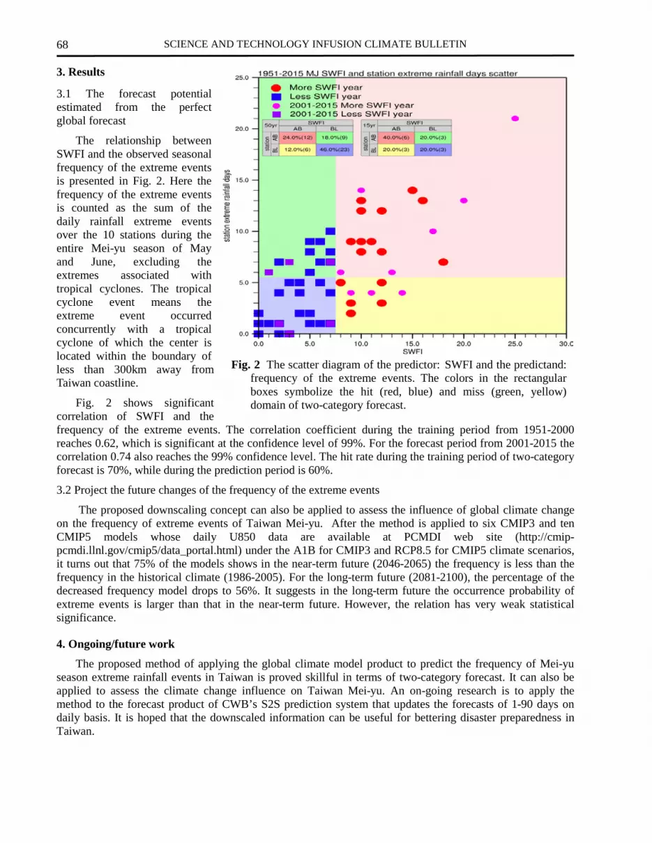
SCIENCE AND TECHNOLOGY INFUSION CLIMATE BULLETIN
68
3. Results
3.1 The forecast potential estimated from the perfect global forecast
The relationship between SWFI and the observed seasonal frequency of the extreme events is presented in Fig. 2. Here the frequency of the extreme events is counted as the sum of the daily rainfall extreme events over the 10 stations during the entire Mei-yu season of May and June, excluding the extremes associated with tropical cyclones. The tropical cyclone event means the extreme event occurred concurrently with a tropical cyclone of which the center is located within the boundary of less than 300km away from Taiwan coastline.
Fig. 2 shows significant correlation of SWFI and the frequency of the extreme events. The correlation coefficient during the training period from 1951-2000 reaches 0.62, which is significant at the confidence level of 99%. For the forecast period from 2001-2015 the correlation 0.74 also reaches the 99% confidence level. The hit rate during the training period of two-category forecast is 70%, while during the prediction period is 60%.
3.2 Project the future changes of the frequency of the extreme events
The proposed downscaling concept can also be applied to assess the influence of global climate change on the frequency of extreme events of Taiwan Mei-yu. After the method is applied to six CMIP3 and ten CMIP5 models whose daily U850 data are available at PCMDI web site (http://cmip-pcmdi.llnl.gov/cmip5/data_portal.html) under the A1B for CMIP3 and RCP8.5 for CMIP5 climate scenarios, it turns out that 75% of the models shows in the near-term future (2046-2065) the frequency is less than the frequency in the historical climate (1986-2005). For the long-term future (2081-2100), the percentage of the decreased frequency model drops to 56%. It suggests in the long-term future the occurrence probability of extreme events is larger than that in the near-term future. However, the relation has very weak statistical significance.
4. Ongoing/future work
The proposed method of applying the global climate model product to predict the frequency of Mei-yu season extreme rainfall events in Taiwan is proved skillful in terms of two-category forecast. It can also be applied to assess the climate change influence on Taiwan Mei-yu. An on-going research is to apply the method to the forecast product of CWB’s S2S prediction system that updates the forecasts of 1-90 days on daily basis. It is hoped that the downscaled information can be useful for bettering disaster preparedness in Taiwan.
Fig. 2 The scatter diagram of the predictor: SWFI and the predictand: frequency of the extreme events. The colors in the rectangular boxes symbolize the hit (red, blue) and miss (green, yellow) domain of two-category forecast.

LU ET AL.
69
References
Kalnay, E., and Coauthors, 1996: The NCEP/NCAR 40-year reanalysis project. Bull. Amer. Meteor. Soc., 77, 437–471.
Saha, S. and Coauthors, 2010: The NCEP climate forecast system reanalysis. Bull. Amer. Meteor. Soc., 91, 1015-1057.
Wang, S.-Y., Y.-H. Lin, and C.-H. Wu, 2015: Interdecadal shift of the active-phase East Asian summer monsoon (Meiyu). Atmospheric Science Letters, doi: 10.1002/asl.603.
Yim, S.-Y., B. Wang, W. Xing, and M.-M. Lu, 2015: Prediction of Meiyu rainfall in Taiwan by multi-lead physical-empirical models. Clim. Dyn., 44, 3033-3042. doi:10.1007/s00382-014-2340-0.

Science and Technology Infusion Climate Bulletin
NOAA’s National Weather Service
40th NOAA Annual Climate Diagnostics and Prediction Workshop
Denver, CO, 26-29 October 2015
______________
Correspondence to: Lindsey N. Long, 5830 University Research Court, Climate Prediction Center, NOAA/NWS/NCEP,
College Park, Maryland; E-mail: [email protected]
Intraseasonal Tropical Storm Prediction in the NCEP CFSv2 45-Day Forecasts
Lindsey N. Long1,2
, Jae-Kyung E. Schemm1, Stephen Baxter
1
1Climate Prediction Center, NOAA/NWS/NCEP, College Park, Maryland 2Innovim LLC, Greenbelt, Maryland
1. Introduction and motivation
The majority of tropical storm (TS) forecasts focus on either the short-term (1-5 days) or the seasonal
aspect by ocean basin. Although studies have shown predictability at the intraseasonal timescale using
mechanisms such as the Madden Julian Oscillation (MJO) (Maloney and Hartmann, 2000; Klotzbach, 2010),
there are few products which attempt to utilize these signals to produce operational products. With the
availability of the Climate Forecast System Version 2 (CFSv2) 45-Day forecasts, the ability to forecast at the
intraseasonal timescale can be more thoroughly examined. Because the CFS is a fully-coupled climate
system, it is well equipped to handle forecasts out to weeks 1 to 4.
The Climate Prediction Center (CPC) currently issues the Global Tropics Hazards and Benefits (GTHB)
Outlook (http://www.cpc.ncep.noaa.gov/products/precip/CWlink/ghazards/), which produces forecasts for
tropical precipitation and TS formation globally for weeks 1 and 2. Shaded regions indicate either high or
moderate confidence of TS formation and weekly total rainfall in the upper/lower third of the historical range.
This product is released each Tuesday and contains both a graphical representation of this information and a
detailed discussion. During the active TS season for the Northern Hemisphere (June 1st – November 30
th), the
outlook is also updated on Friday for a limited region (120°E-0° and 0°-40°N) which encompasses the
Atlantic and both the Eastern and Western North Pacific basins.
The shaded areas in the GTHB Outlook, which represent areas with favorable conditions for tropical
cyclogenesis, are determined subjectively based on a few forecasts tools. With the creation of a year-round
forecast of TSs for Weeks 1-4 by CFSv2, we hope to provide these forecasters with an objective tool for the
Outlook. It may also assist in the possible expansion to include Week 3 in the Outlook.
2. Data and tracking methods
a) CFSv2 45-day forecasts
The CFSv2 is a fully coupled atmosphere-ocean-land model run operationally at the National Centers for
Environmental Prediction (NCEP) since April 2011 (Saha et al. 2014). The CFSv2 45-Day forecasts are
currently run four times daily at the 00Z, 06Z, 12Z, and 18Z cycles with four ensemble members each. The
sixteen members created daily have output saved every six hours. A 14-year hindcast has also been produced
for 1999-2012 with only one member for each of the four initializations. Because of the sparse number of
daily ensemble members in the hindcasts, the five days prior to the forecasted day are used to create a more
robust 20-member ensemble. For verification, observations from the National Hurricane Center (NHC) and
the Joint Typhoon Warning Center’s (JTWC) Best-Track datasets are utilized. Since the 2015 best-track data
are not yet available, the advisories from operational centers are used for corresponding basins.
b) TS tracking and filtering
The detection and tracking method used in this study is based on the algorithm created by Camargo and
Zebiak (2002). With this method, a point must meet seven criteria in order to be considered a TS. Many of
the thresholds used in the criteria are basin and model-dependent. The seven basins used in this study are the
Atlantic (ATL), eastern North Pacific (ENP), western North Pacific (WNP), North Indian (NI), South Indian
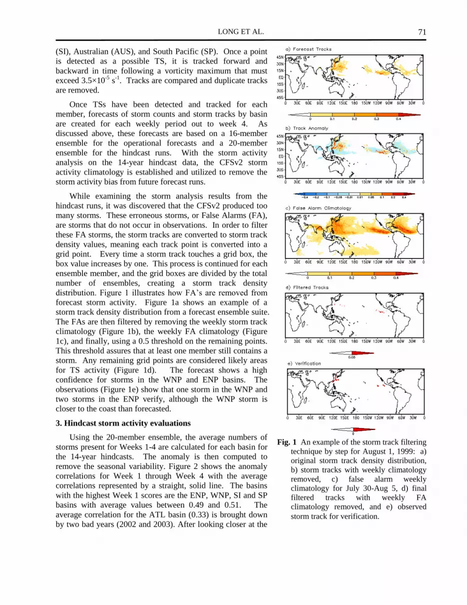
LONG ET AL.
71
(SI), Australian (AUS), and South Pacific (SP). Once a point
is detected as a possible TS, it is tracked forward and
backward in time following a vorticity maximum that must
exceed 3.5×10⁻⁵
s-1
. Tracks are compared and duplicate tracks
are removed.
Once TSs have been detected and tracked for each
member, forecasts of storm counts and storm tracks by basin
are created for each weekly period out to week 4. As
discussed above, these forecasts are based on a 16-member
ensemble for the operational forecasts and a 20-member
ensemble for the hindcast runs. With the storm activity
analysis on the 14-year hindcast data, the CFSv2 storm
activity climatology is established and utilized to remove the
storm activity bias from future forecast runs.
While examining the storm analysis results from the
hindcast runs, it was discovered that the CFSv2 produced too
many storms. These erroneous storms, or False Alarms (FA),
are storms that do not occur in observations. In order to filter
these FA storms, the storm tracks are converted to storm track
density values, meaning each track point is converted into a
grid point. Every time a storm track touches a grid box, the
box value increases by one. This process is continued for each
ensemble member, and the grid boxes are divided by the total
number of ensembles, creating a storm track density
distribution. Figure 1 illustrates how FA’s are removed from
forecast storm activity. Figure 1a shows an example of a
storm track density distribution from a forecast ensemble suite.
The FAs are then filtered by removing the weekly storm track
climatology (Figure 1b), the weekly FA climatology (Figure
1c), and finally, using a 0.5 threshold on the remaining points.
This threshold assures that at least one member still contains a
storm. Any remaining grid points are considered likely areas
for TS activity (Figure 1d). The forecast shows a high
confidence for storms in the WNP and ENP basins. The
observations (Figure 1e) show that one storm in the WNP and
two storms in the ENP verify, although the WNP storm is
closer to the coast than forecasted.
3. Hindcast storm activity evaluations
Using the 20-member ensemble, the average numbers of
storms present for Weeks 1-4 are calculated for each basin for
the 14-year hindcasts. The anomaly is then computed to
remove the seasonal variability. Figure 2 shows the anomaly
correlations for Week 1 through Week 4 with the average
correlations represented by a straight, solid line. The basins
with the highest Week 1 scores are the ENP, WNP, SI and SP
basins with average values between 0.49 and 0.51. The
average correlation for the ATL basin (0.33) is brought down
by two bad years (2002 and 2003). After looking closer at the
Fig. 1 An example of the storm track filtering
technique by step for August 1, 1999: a)
original storm track density distribution,
b) storm tracks with weekly climatology
removed, c) false alarm weekly
climatology for July 30-Aug 5, d) final
filtered tracks with weekly FA
climatology removed, and e) observed
storm track for verification.

SCIENCE AND TECHNOLOGY INFUSION CLIMATE BULLETIN
72
storm counts in the basin’s subregions and also wind shear anomalies, it was found that the forecasts in the
subtropical, Northern Atlantic accounted for these low scores. As expected, skill drops with lead time, but
there is still skill evident in most basins for Weeks 2-4 with scores for Week 4 remaining above 0.2.
Fig. 2 Tropical storm count anomaly correlations by week for the a) Atlantic, b) Eastern North Pacific, c)
Western North Pacific, and d) North Indian basins for 1999-2012, and the e) South Indian, f) Australian,
and g) South Pacific basins for 2000-2012. Because the 1999 SH season begins in 1998, it is not included.
The average correlation is shown using a straight, solid line.

LONG ET AL.
73
Fig. 3 Heidke skill scores for filtered storm tracks by week for the a) Atlantic, b) Eastern North Pacific, c)
Western North Pacific, and d) North Indian basins for 1999-2012 (solid lines), and the e) South Indian, f)
Australian, and g) South Pacific basins for 2000-2012 (solid lines). Dotted lines are for the real-time evaluation
from 2014-2015.
After performing the filtering described above, the Heidke Skill Scores (HSS) are computed for the storm
tracks in each basin. Because of the nature of the HSS, months with no storms will have a score of zero. No
credit is given for a correct forecast of zero storms when there is also a verification of zero storms. Skill is
achieved through the correct forecast of a storm track (Hits). Therefore, as expected, skill scores increase

SCIENCE AND TECHNOLOGY INFUSION CLIMATE BULLETIN
74
with increased seasonal activity. Figure 3 shows the HSS for each weekly lead by basin (solid lines). The
highest Week 1 scores are present in the ATL, ENP and WNP basins, with scores between 0.25 and 0.35
during the most active part of the season. The SI and AUS basins show an increase in scores during the latter
half of the season instead of during the peak in the seasonal cycle for these basins. This indicates the model is
either missing the observed storms or producing too many FAs during these months. Skill scores for Week 2
decrease, but they then remain steady for Weeks 3 and 4.
Fig. 4 Genesis lag day plots by week for the a) Atlantic, b) Eastern North Pacific, c) Western North Pacific, d)
North Indian basins, e) South Indian, f) Australian, and g) South Pacific basins averaged for each storm
from 1999-2012. The black vertical line indicates the day of genesis (Lag Day 0).

LONG ET AL.
75
Fig. 5 Same as Figure 4, but for the 2014-2015 real-time evaluation. Numbers in parentheses indicate the total
number of observed storms for the 2-year period.
Another way to view the model’s skill in forecasting storm track is to compare the number of grid point
hits (model and observations both showing a storm present) as a lag from the genesis point for individual
storms. Unlike the HSS, this takes into account only hits or misses by the model and not FAs. Figure 4
shows this lag as a percentage of model hits versus the total possible hits for all storms in a basin during the
14-year period. The genesis day (Lag day 0) is highlighted with a vertical black line. During Week 1, the
storm is included in the model’s initial conditions (IC) starting at day 0. Therefore, negative lags (left of the
black line) forecast both track and cyclogenesis, while positive lags (right of the black line) forecast only the

SCIENCE AND TECHNOLOGY INFUSION CLIMATE BULLETIN
76
track. For weeks 2-4, the entire period is forecasting both track and cyclogenesis with the exception of a
storm that lasts over seven days. In this case, the storm is present in the ICs for the 7th and 8
th lag day of
Week 2.
Because of the influence of the ICs in Week 1, the percentage of hits, or hit rate, increases once the TS
has formed (Figure 4). However, there is still considerable skill during the negative lags, most notably in the
NI and Southern Hemisphere (SH) basins. This indicates that the lower skill in the HSSs for these basins is
due to a high number of FA storms and not a missed forecast of observed storms. The NI and SP basins also
show promise during Week 2. The opposite is true for the ATL, ENP, and WNP during the longer leads.
Although the HSS shows higher scores for weeks 2-4 in these basins, the hit rate is very low, indicating more
misses of observed storms and less FAs.
4. Real-time forecasting
In December 2013, ongoing,
real-time prediction began using the
16-member operational runs
described above. Because this began
in the middle of the SH season, the
results described below for the 2014
season are for January 1-May 30 only
for the SH basins. The storm count
anomaly correlations are given in
Table 1. Numbers in bold represent
those above the hindcast average seen
in Figure 2. Because all sixteen
ensemble members use ICs within a
24-hour period versus the five-day
average of ensemble members needed for the hindcast runs, higher values are expected; however, this is not
true for all basins. The WNP basin is the only basin with higher values for all weekly leads. The ATL and
ENP basins also have many weekly leads above the hindcast average, with more occurring in 2014. The
basins in the SH and the NI basin show mostly lower skill than the hindcasts runs, meaning there is little
improvement with decreased lead time.
The dotted lines in Figure 3 represent the HSSs for the 2014-2015 operational evaluation. For most of the
basins, the scores increase in magnitude, but overall show a similar pattern. The biggest score increases occur
in the ENP, NI and AUS basins. The highest scores for AUS remain in the latter part of the season, peaking
in March, while the highest scores for SI tend to shift more towards January, the peak in the seasonal cycle.
Although the genesis lag day plots for the 2014-2015 forecasts (Figure 5) are much noisier than those for
the 14-year hindcast runs, they are overall very similar in structure. There is, however, increased skill for the
real-time prediction in every basin at each weekly lead except for the ATL basin. These results are consistent
with the increased HSS. An interesting point to note is that although the SI and AUS basins show relatively
good skill in predicting the observed storms in the genesis lag day plots, the count correlations are relatively
low except for the early week leads for the SI basin in 2014. This indicates an abundance of FAs still
remaining in these basins.
5. Conclusion
With the availability of the CFSv2 45-day runs at NCEP, a new product on TS intraseasonal prediction
has been developed to assist CPC forecasters. This product provides guidance on both storm count and storm
location. Although skill drops with lead time, Weeks 2-4 still show skill for both storm count and storm
track. Real-time experimental predictions for the 2014 and 2015 seasons show increased skill for many
basins. It indicates predictability for the ATL, ENP and WNP basins, while the SH basins still struggle with
FAs. This product is currently available as a non-operational product on the CPC ftp site at:
ftp://ftp.cpc.ncep.noaa.gov/llong/main.html. Comments and suggestions are always welcome.
Year Week ATL ENP WNP NI SI AUS SP
2014
Week 1 0.49 0.36 0.76 0.24 0.72 0.06 0.25
Week 2 0.43 0.45 0.55 0.14 0.53 -0.28 0.34
Week 3 0.26 0.36 0.39 0.05 0.06 -0.37 0.37
Week 4 0.27 0.31 0.41 -0.04 -0.13 -0.30 0.29
2015
Week 1 0.32 0.49 0.63 0.43 0.36 0.36 0.52
Week 2 0.12 0.33 0.74 0.16 0.19 0.30 0.27
Week 3 0.10 0.21 0.47 -0.04 0.13 0.05 0.03
Week 4 0.08 0.12 0.32 -0.05 0.18 -0.19 -0.03
Table 1 Storm track count anomaly correlations for 2014 and 2015
during the active seasons. For 2014, SH basin correlations are for
the shortened forecast period Jan 1 - May 31. Bold values are for
those higher than the climatological value.

LONG ET AL.
77
Acknowledgements. This study was partially supported by NOAA's Climate Program Office's Modeling,
Analysis, Predictions, and Projections program.
References
Camargo, S.J., and S.E. Zebiak, 2002: Improving the detection and tracking of tropical cyclones in
atmospheric general circulation models. Wea. Forecasting, 17, 1152-1162.
Klotzbach, P.J., 2010: On the Madden-Julian oscillation-Atlantic hurricane relationship. J. Climate, 23, 282-
293.
Maloney E.D., and D.L. Hartmann, 2000: Modulation of hurricane activity in the Gulf of Mexico by the
Madden-Julian oscillation, Science, 287, 2002-2004.
Saha, S., and Coauthors, 2014: The NCEP Climate Forecast System version 2. J. Climate, 27, 2185–2208.

4. PREDICTION OF ENSO ANDITS REMOTE IMPACTS
40th NOAA Climate Diagnostics and Prediction Workshop

Science and Technology Infusion Climate Bulletin
NOAA’s National Weather Service
40th NOAA Annual Climate Diagnostics and Prediction Workshop
Denver, CO, 26-29 October 2015
______________
Correspondence to: Li-Chuan Chen, ESSIC/CICS-MD, University of Maryland, 5830 University Research Court,
College Park, MD 20740; E-mail: [email protected].
ENSO Precipitation and Temperature Forecasts in the North American
Multi-Model Ensemble: Composite Analysis and Validation
Li-Chuan Chen1,2
, Huug van den Dool2, Emily Becker
2,3, and Qin Zhang
2
1Earth System Science Interdisciplinary Center/Cooperative Institute for Climate and Satellites,
University of Maryland, College Park, MD 2Climate Prediction Center, NCEP/NWS/NOAA, College Park, MD
3Innovim, LLC., Greenbelt, MD
1. Introduction
The El Niño/Southern Oscillation (ENSO) has a large influence on the seasonal precipitation (P) and
temperature (T) patterns over the United States and across the globe (Ropelewski and Halpert 1986, 1987;
Trenberth et al. 1998; Dai and Wigley 2000). At NOAA Climate Prediction Center (CPC), a large effort is
devoted to monitoring and forecasting of Niño-3.4 sea surface temperature (SST) and the tropical Pacific
Ocean conditions, in order to provide the most up-to-date information on the phase of the ENSO cycle.
Statistical tools have been developed for objective seasonal prediction using Niño-3.4 SST forecasts in
conjunction with observed P and T composites keyed to phases of the ENSO cycle (Higgins et al. 2004). On
the other hand, many studies (e.g., Kumar et al. 1996; Mathieu et al. 2004) have shown that improved skill of
P and T prediction in climate models can be attributed to the known impacts of ENSO signals, especially
during the Northern Hemisphere cold season. Recent developments in multi-model ensembles provide a
promising way to increase P and T predictive skill using dynamical model forecasts (Graham et al. 2000;
Kirtman et al. 2014).
In this study, we examine P and T forecasts during ENSO events in six models in the North American
Multi-Model Ensemble (NMME), including the CFSv2, CanCM3, CanCM4, FLOR, GEOS5, and CCSM4
models, by comparing the model-based ENSO composites to the observed. The composite analysis is
conducted using the 1982-2010 hindcasts for each of the six models with selected ENSO episodes based on
the seasonal Ocean Niño Index (ONI) just prior to the date the forecasts were initiated. Two types of
composites are constructed over the North American continent: one based on mean precipitation and
temperature anomalies in physical units, the other based on their probability of occurrence in a three-class
forecast system. They are referred as anomaly and probability composites, respectively, hereafter. The
composites apply to monthly mean conditions in November, December, January, February, and March,
respectively, as well as to the five-month aggregates (NDJFM) representing the winter conditions. For
anomaly composites, we use the anomaly correlation coefficient (ACC) and root-mean-square error (RMSE)
against the observed composites for evaluation. For probability composites, we develop a probability anomaly
correlation (PAC) measure and a root-mean probability score (RMPS) for assessment (Chen et al. 2016).
2. ENSO composites
a. Anomaly composites
For each model, monthly ensemble mean P and T forecasts are first obtained by averaging all members.
The P and T anomalies for a given start and lead times are then computed as the difference between the
ensemble mean P and T forecasts and the lead-specific model climatology derived from the hindcast mean of
all members and all years excluding the forecast year. The P and T anomaly composites for the warm ENSO
(El Niño) events and cold ENSO (La Niña) events are simply the average of the ensemble P and T anomaly
maps of selected years. The years are chosen based on the historical ONI published on the CPC website at
http://www.cpc.ncep.noaa.gov/products/analysis_monitoring/ensostuff/ensoyears.shtml. If the seasonal ONI
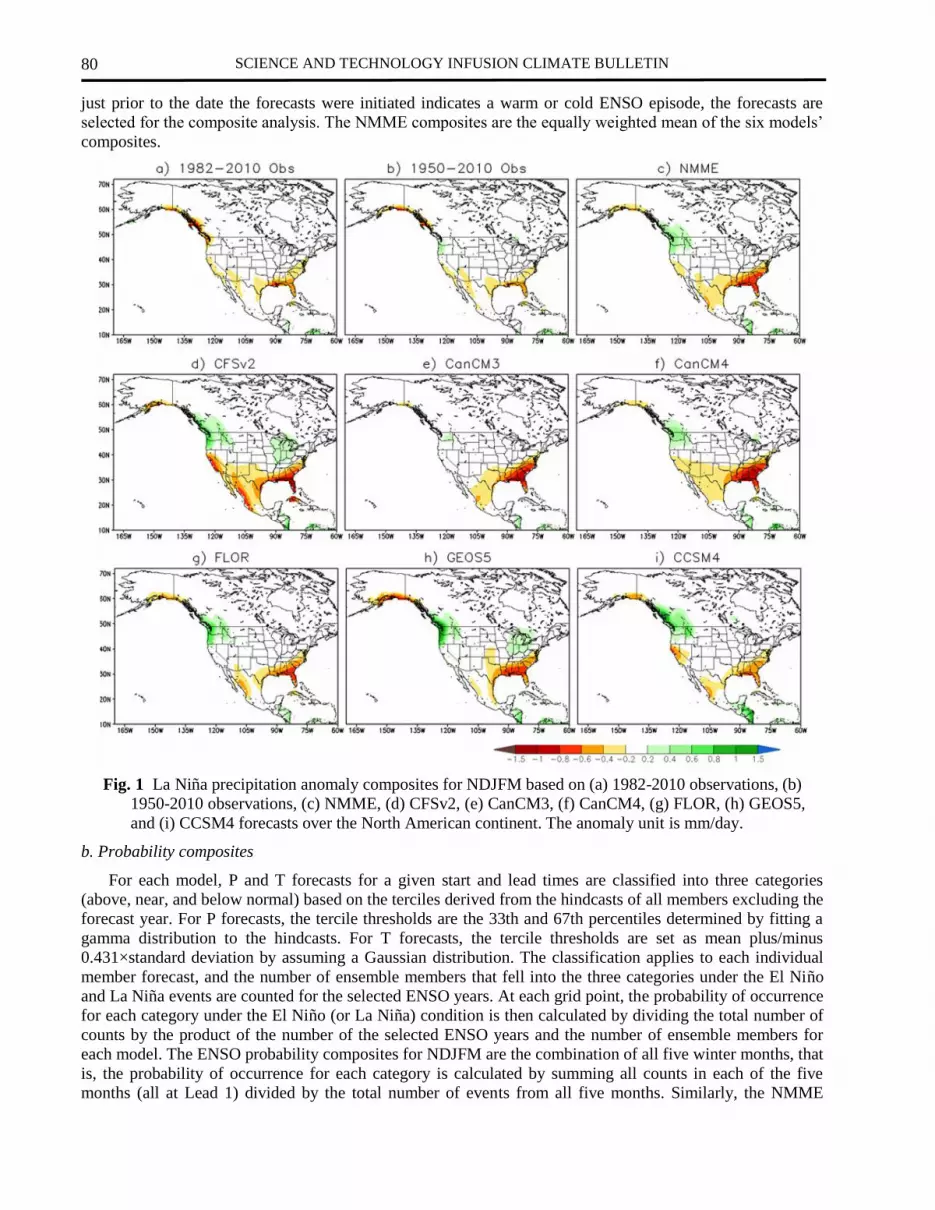
SCIENCE AND TECHNOLOGY INFUSION CLIMATE BULLETIN
80
just prior to the date the forecasts were initiated indicates a warm or cold ENSO episode, the forecasts are
selected for the composite analysis. The NMME composites are the equally weighted mean of the six models’
composites.
Fig. 1 La Niña precipitation anomaly composites for NDJFM based on (a) 1982-2010 observations, (b)
1950-2010 observations, (c) NMME, (d) CFSv2, (e) CanCM3, (f) CanCM4, (g) FLOR, (h) GEOS5,
and (i) CCSM4 forecasts over the North American continent. The anomaly unit is mm/day.
b. Probability composites
For each model, P and T forecasts for a given start and lead times are classified into three categories
(above, near, and below normal) based on the terciles derived from the hindcasts of all members excluding the
forecast year. For P forecasts, the tercile thresholds are the 33th and 67th percentiles determined by fitting a
gamma distribution to the hindcasts. For T forecasts, the tercile thresholds are set as mean plus/minus
0.431×standard deviation by assuming a Gaussian distribution. The classification applies to each individual
member forecast, and the number of ensemble members that fell into the three categories under the El Niño
and La Niña events are counted for the selected ENSO years. At each grid point, the probability of occurrence
for each category under the El Niño (or La Niña) condition is then calculated by dividing the total number of
counts by the product of the number of the selected ENSO years and the number of ensemble members for
each model. The ENSO probability composites for NDJFM are the combination of all five winter months, that
is, the probability of occurrence for each category is calculated by summing all counts in each of the five
months (all at Lead 1) divided by the total number of events from all five months. Similarly, the NMME

CHEN ET AL.
81
probability composites are the combination of all six models by adding all counts in each category from the
six models together, but note that the classification of each model is determined separately in respect to
model’s own hindcast distribution for a particular month.
Fig. 2 El Niño temperature probability composites for NDJFM based on (a) 1982-2010 observations, (b)
1950-2010 observations, (c) NMME, (d) CFSv2, (e) CanCM3, (f) CanCM4, (g) FLOR, (h) GEOS5, and
(i) CCSM4 forecasts over the North American continent.
3. Composite analysis and validation
Figure 1 shows the La Niña P anomaly composites for NDJFM based on 1982-2010 and 1950-2010
observations, NMME, and the six models. All model and the 1950-2010 observed composites present drier
than normal conditions over the southern U.S. and enhanced rainfall over the Pacific Northwest, consistent
with the pattern suggested by Ropelewski and Halpert (1986, 1987). The 1982-2010 observed NDJFM P
anomaly composite also displays similar La Niña pattern to the 1950-2010 observed. In contrast to the
NMME and 1950-2010 observed composites, the 1982-2010 observed has below-normal rainfall over the
Pacific Northwest, likely a sampling error due to small sample size. There are some variations among the six
models but all models are reasonably good. CFSv2 has the biggest North-South contrast in the anomalies and
its dry area is spread farther into central Mexico, while both CanCM models produce large negative deviation
over the southeastern U.S. Despite the subtle differences, the remarkable similarity between the NMME and
observed P anomaly composites under both El Niño (not shown) and La Niña conditions demonstrates the

SCIENCE AND TECHNOLOGY INFUSION CLIMATE BULLETIN
82
significant progress in ENSO-precipitation relationships from seasonal dynamical models since Smith and
Ropelewski (1997).
Fig. 3 ACC of all models and months for (a) El Niño precipitation anomaly composites, (b) La Niña
precipitation anomaly composites, (c) El Niño temperature anomaly composites, and (d) La Niña
temperature anomaly composites, validated with 1950-2010 observations.
Figure 2 presents the El Niño T probability composites for NDJFM based on 1982-2010 and 1950-2010
observations, NMME, and the six models. Unlike the observed P composites, there are larger differences
between the 1982-2010 and 1950-2010 observed T probability composites. The 1982-2010 observed
composite has bigger warm-cold (North-South) contrast, and its below-normal area is centered over Texas

CHEN ET AL.
83
and northern Mexico and does not cover the southeast U.S. Similar to the findings from the T anomaly
composites (not shown), T probability composites vary greatly with model. GEOS5, CanCM4, and FLOR
models have the largest deviations and are the main contributors to the difference between the NMME and
observed probability composites.
In order to present a quantitative evaluation of how well NMME models predict P and T patterns under
ENSO conditions, we compute the ACC and RMSE for P and T anomaly composites, and PAC and RMPS
for P and T probability composites (Chen et al. 2016). Figure 3 shows the matrix charts of ACC for all models
and months, including NMME and NDJFM, using the 1950-2010 observations for validation. Several features
are worth highlighting in Figure 3. First, the fidelity is generally higher for NMME composites, as well as
NDJFM composites, though a given model at a given month may have slightly larger ACC score. Second,
predictive skill varies with month. All models, as well as NMME, have greater ACC for February prediction,
and this is seen for both P and T anomaly composites under either El Niño or La Niña condition. Third, most
models perform marginally better in predicting El Niño P and T anomaly patterns than La Niña patterns.
Fourth and last, CFSv2 is the overall best individual model in predicting ENSO P and T patterns during
wintertime. The findings from the RMSE for anomaly composites and PAC and RMPS for probability
composites are similar to the ACC results. However, PAC is able to discriminate the performance between the
P and T prediction more and shows larger scores for P probability composites than T probability composites
under both El Niño and La Niña conditions.
4. Summary and conclusions
We have compared and validated precipitation and temperature forecasts under ENSO conditions in six
NMME models with long-term climate observations. Our aim is to understand whether coupled seasonal
dynamical models can adequately predict ENSO’s impacts on North American precipitation and temperature
patterns while an El Niño or La Niña event is in progress. We focus on the overall model performance, and
provide a comprehensive analysis and validation of both the anomaly and probability composites constructed
from selected warm or cold ENSO episodes based on the tropical Pacific Ocean conditions during the
Northern Hemisphere winter season. The key findings from the study are summarized below.
• NMME predicts ENSO precipitation patterns well during wintertime. All models are reasonably good.
CFSv2 performs particularly well. This result gives us confidence in NMME precipitation forecasts
during an ENSO episode and models’ ability in simulating teleconnections.
• There are some discrepancies between the NMME and observed composites for temperature forecasts,
in terms of both magnitude and spatial distribution. The differences are mainly contributed by the
GEOS5, CanCM4, and FLOR models, and thus the NMME aggregates have difficulties in reproducing
the ENSO-temperature relationships.
• For all ENSO precipitation and temperature composites, the fidelity is greater for the multi-model
ensemble, as well as the five-month aggregates. February tends to have higher performance score than
other winter months.
• For anomaly composites, most models perform slightly better in predicting El Niño patterns than La
Niña patterns.
• For probability composites, all models have superior performance in predicting ENSO precipitation
patterns than temperature patterns.
A full-length technical paper (Chen et al. 2016) documenting details of this study has been submitted to
Journal of Climate for publication. The complete set of ENSO composites for all models and months
(including all the figures not shown in this abstract), along with global composites, are available on CPC
NMME website at http://www.cpc.ncep.noaa.gov/products/NMME/enso/.
Acknowledgements. We gratefully acknowledge the usage of the NMME Phase 1 and 2 data. The
NMME Project and data dissemination is supported by NOAA, NSF, NASA and DOE. We thank the climate
modeling groups for producing and making available their model output. NOAA NCEP, NOAA Climate Test

SCIENCE AND TECHNOLOGY INFUSION CLIMATE BULLETIN
84
Bed and NOAA Climate Program Office jointly provide coordinating support and the NMME data archives
are maintained by IRI and NCAR.
References
Chen, L.-C., H. van den Dool, E. Becker, and Q. Zhang, 2016: ENSO precipitation and temperature forecasts
in the North American Multi-Model Ensemble: Composite analysis and validation. J. Climate, in review.
Dai, A., and T. M. L. Wigley, 2000: Global patterns of ENSO-induced precipitation. Geophys. Res. Lett., 27,
1283-1286.
Graham, R. J., A. Evans, K. Mylne, M. Harrison, and K. Robertson, 2000: An assessment of seasonal
predictability using atmospheric general circulation models. Quart. J. Roy. Meteor. Soc., 126, 2211-2240.
Higgins, R. W., H.-K. Kim, and D. Unger, 2004: Long-lead seasonal temperature and precipitation prediction
using tropical Pacific SST consolidation forecasts. J. Climate, 17, 3398-3414.
Kirtman, B. P., and Coauthors, 2014: The North American Multi-Model Ensemble (NMME): Phase-1
seasonal to interannual prediction, phase-2 toward developing intra-seasonal prediction. Bull. Amer.
Meteor. Soc., 95, 585-601, doi: 10.1175/BAMS-D-12-00050.1.
Kumar, A., M. Hoerling, M. Leetma, and P. Sardeshmukh, 1996: Assessing a GCM’s suitability for making
seasonal predictions. J. Climate, 9, 115-129.
Mathieu, P.-P., R. T. Sutton, B. Dong, and M. Collins, 2004: Predictability of winter climate over the North
Atlantic European region during ENSO events. J. Climate, 17, 1953-1974.
Ropelewski, C. F., and M. S. Halpert, 1986: North American precipitation and temperature patterns
associated with the El Niño/Southern Oscillation. Mon. Wea. Rev., 114, 2352-2362.
Ropelewski, C. F., and M. S. Halpert, 1987: Global and regional scale precipitation patterns associated with
the El Niño/Southern Oscillation. Mon. Wea. Rev., 115, 1606–1625.
Smith, T. M., and C. F. Ropelewski, 1997: Quantifying Southern Oscillation–precipitation relationships from
an atmospheric GCM. J. Climate, 10, 2277–2284.
Trenberth, K. E., G. Branstator, D. Karoly, A. Kumar, N. Lau, and C. Ropelewski, 1998: Progress during
TOGA in understanding and modeling global teleconnections associated with tropical sea surface
temperatures. J Geophys. Res., 103, 14291-14324.

Science and Technology Infusion Climate Bulletin NOAA’s National Weather Service 40th NOAA Annual Climate Diagnostics and Prediction Workshop Denver, CO, 26-29 October 2015
______________
Correspondence to: Jieshun Zhu, 5830 University Research Ct., Climate Prediction Center, NOAA/NWS/NCEP, College Park, Maryland; E-mail: [email protected].
The Relationship between Thermocline Depth and SST Anomalies in the Eastern Equatorial Pacific: Seasonality and Decadal Variations
Jieshun Zhu1,2, Arun Kumar1, and Bohua Huang3,4 1Climate Prediction Center, NOAA/NWS/NCEP, College Park, Maryland
2 Innovim, Greenbelt, Maryland 3Department of Atmospheric, Oceanic, and Earth Sciences, College of Science,
George Mason University, Fairfax, Virginia 4Center for Ocean-Land-Atmosphere Studies, George Mason University, Fairfax, Virginia
ABSTRACT
Even though the vital role of thermocline fluctuation in ENSO cycle has been established previously, the direct relationship between the thermocline depth and SST anomalies in the equatorial Pacific is yet to be fully understood, especially its seasonality. Thermocline depth anomalies were found to lead SST anomalies in time with a longitude-dependent delay, but our study suggests that the relationship shows strong seasonal dependency, which is the most (least) significant during the boreal spring (summer). Over the eastern
equatorial Pacific where there is the least delay comparing with western and central Pacific, the connection between thermocline and SST is the weakest during the boreal spring (Fig. 1). This feature is one of origins for ENSO spring persistence barrier, as evidenced by the weakest thermocline and Bjerknes feedbacks occurring in spring (Fig. 2). Furthermore, the thermocline-SST connections exhibit significant decadal variations, which are remarkably consistent with the decadal changes in the persistence barrier of SST anomalies over the eastern Pacific. It is also found that the decadal shift in the timing of the thermocline-SST connection barrier is caused by the
Fig. 1 Lead-lag correlations between observed Z20 and SST anomalies for (a) all months regardless of season, (c) January, (d) April, (e) July and (f) October. (b) Simultaneous correlations between observed Z20 and SST anomalies as a function of season. Positive lag means Z20 leads SST. All calculations are based on 1982-2011 and presented along the equator (averaged over 2ºS-2ºN).

SCIENCE AND TECHNOLOGY INFUSION CLIMATE BULLETIN
86
changes in the seasonal cycle of tropical trade winds and thermocline depths (Fig. 3).
This work has been published in Geophysical Research Letters in 2015.
References
Zhu, J., A. Kumar, and B. Huang, 2015: The relationship between thermocline depth and SST anomalies in the eastern equatorial Pacific: Seasonality and decadal variations. Geophys. Res. Lett., 42, 4507–4515. doi: 10.1002/2015GL064220.
Fig. 2 Simultaneous correlations as a function of season between the observed Z20 and SST anomalies averaged over the Niño3 region (red curve), and between the observed SST zonal gradients and the surface zonal wind stress anomalies averaged over the Niño 4 region (black curve). The SST zonal gradient is defined as the difference between the western Pacific region (120ºE-160ºE, 5ºS-5ºN) and the Niño 3 region. Calculations are performed for 1982-2011.
Fig. 3 Simultaneous correlations between Z20 and SST anomalies averaged over the Niño3 region as a function of season within an 11-year moving window, with SST data from ERSST3 and Z20 data from (a) ORA-S3, (b) ORA-S4 and (c) SODA. (d) Seasonality of Niño3 SST anomalies persistence within an 11-year moving window. The persistence for a given month (e.g., March) is defined as the correlation between two time series for one month earlier (February) and later (April) than the month. The 11-year window is shifted year by year from 1958 to 2013.

Science and Technology Infusion Climate Bulletin NOAA’s National Weather Service 40th NOAA Annual Climate Diagnostics and Prediction Workshop Denver, CO, 26-29 October 2015
______________
Correspondence to: Schaler R. Perry, Surfline/Wavetrak, Inc., 300 Pacific Coast HWY Suite 310, Huntington Beach, CA 92648; E-mail: [email protected]
Global ENSO Ocean Wave Trends During the Last 30 Years
Schaler R. Perry1 and Mark Willis2 1Surfline/Wavetrak, Inc. World Headquarters, Huntington Beach, CA
2Surfline/Wavetrak, Inc., Nags Head, NC
Surfline celebrated 30 years of delivering surf reports and forecasts in 2015. The company has grown from an organization that initially produced surf reports and forecasts solely in Southern California in 1985 to a global marine, surf, and fish forecasting and editorial solution. The last 30 years of acquiring surf and swell observations have uniquely positioned us to analyze long term wave climate trends on a global scale.
This is an overview of Surfline’s historical wave data, presented as it relates to the warm phases of the El Niño Southern Oscillation. The data presented in the plots for specified locations are daily mean significant wave height values (m) for the given months and year. The affects of El Niño on the Northern Hemisphere winter have been covered quite extensively, and plots from both the North Pacific and North Atlantic provide fairly clear, expected signals for many locations (Fig. 1).
Looking back through 30+ years of wind and wave data, the seasonal predictors associated with moderate and especially strong El Niño events are quite clear. During the winter peak, most notably during strong events, we see an appreciable uptick in swell energy after the holidays during the months of January, February, and March. In terms of the fall and early winter months of October, November, and December, the signal is far less clear. This is represented quite well in the cases of Southern California and New York (Fig. 2, 3). The locations of interest were offshore to the west of Point Conception, and to the southeast of the mouth of the Hudson River, respectively.
As the Southern Hemisphere winter typically bookends the peak of ENSO events, we have highlighted the years pre and post peak to try and better identify possible trends in swell activity. Looking back on swell data for key markets that rely on the fruits of the Southern Hemisphere’s storminess, there were mixed findings. While the signals for the North Pacific, and North Atlantic for that matter, are quite clear for a myriad of destinations, the Southern Hemisphere is not so clear cut.
The impact the warm phase of ENSO has had, and potentially will have, on swell production during the Southern Hemisphere winter has been documented less and is more difficult to discern when looking back through the wave climatology (Fig. 4). That said it is interesting to note the uptick in swell for Fiji preceding the peak in strong El Niño events, likely attributable to increased tradeswell.
For more info on how this impacts the surf in the North Pacific and North Atlantic basins through the winter, please check out our Seasonal Outlooks for each respective basin. They can be found below.
Fig. 1 Average significant wave heights, (a) OND 1982 and (b) JFM 1983.
(a)
(b)

SCIENCE AND TECHNOLOGY INFUSION CLIMATE BULLETIN
88
North Pacific Winter Outlook - http://www.surfline.com/surf-news/heres-what-we-can-expect-for-the-west-coast-hawaii-and-beyond-this-winter-thanks-to-a-robust-el-nino-event-off_133236/
North Atlantic Winter Outlook - http://www.surfline.com/surf-news/a-strong-el-nino-event-is-a-shoo-in-and-likely-to-enhance-surf-for-some-locations-official-15-16-atlantic-wint_133370/
Fig. 2 Average significant wave heights for Southern California, (left) OND and (right) JFM.
Fig. 3 Average significant wave heights for New York, (left) OND and (right) JFM.
Fig. 4 Average Significant Wave Heights for Chile during the Southern Hemisphere winter pre and post peak of moderate to strong El Niño events, (left) Chile, (right) Fiji.

Science and Technology Infusion Climate Bulletin NOAA’s National Weather Service 40th NOAA Annual Climate Diagnostics and Prediction Workshop Denver, CO, 26-29 October 2015
______________
Correspondence to: Luke He, 5830 University Research Court, Climate Prediction Center, NOAA/NWS/NCEP, College Park, Maryland; E-mail: [email protected]@noaa.gov
ENSO and Seasonal Rainfall Variability over the Hawaiian and US-affiliated Pacific Islands
Luke He1 and Pacific Climate Team 1Climate Prediction Center, NOAA/NWS/NCEP, College Park, Maryland
The tropical Pacific region is one of the world’s most vulnerable areas with respect to weather-related natural disasters and extreme hydro-meteorological events. Short-term climate fluctuations, such as the El Niño-Southern Oscillation (ENSO) phenomenon and its recurring warm and cold episodes, are found to play an important role in the climate variability over the Hawaiian and tropical Pacific region.
The influence of ENSO episodes on Pacific Basin precipitation is described in greater detail using composite analysis, in which responses to warm ENSO episodes are considered separately from responses to cold episodes. The degree of realism of the assumption of linearity in the ENSO-rainfall relationship, which is needed in the overall interpretation of the correlations, is evaluated in composite analysis. If rainfall anomaly composites are fairly equal-but-opposite for warm versus cold ENSO conditions, approximate linearity is confirmed. While the resulting set of winters is in general agreement with the sets as defined earlier by Loon and Madden (1981), Rasmusson and Carpenter (1983) and Ropelewski and Jones (1987), a few differences exist.
As an example, Fig. 1 shows ENSO composite rainfall results for Kahului, Hawaii. The differences between the composited rainfall totals for the samples representing the warm or cold phases of ENSO versus the totals of the remaining years (neutral-plus-oppositely phased years) were statistically tested with the Student's t-test. It should be noted that the statistical assumptions underlying the t-test (e.g. Gaussian distributions) may not be sufficiently satisfied. Nonetheless, we use it as a rough guide for indicating significant mean differences in rainfalls as a function of ENSO category. Near the time of the mature episode boreal winter at Kahului, warm episodes are associated with deficient precipitation with 0.05 or stronger statistical significance in Dec-Jan-Feb, Jan-Feb-Mar, Feb-Mar-Apr. Cold episodes associate with slightly enhanced rainfall but not at the 0.05 significance level. More detailed information (e.g., the seasonal variation of the tropical rainfall with ENSO) can be found in the He et al. 1998. Recent study (O'Connor et al. 2015) shows a drying trend in Hawaii rainfall
Fig. 1 Composite rainfall amounts for Kahului, Hawaii, by ENSO status. The dashed line denotes the climatological mean rainfall for all years, the red line the mean for the composited warm ENSO episode years, and the blue line the mean for the cold episode years. Differences between the composited rainfalls for the samples representing the warm phases of ENSO versus that of the remaining (neutral plus cold phase) years passing a 2-tailed significance test at the 0.05 level are indicated with a hollow square along the red line. Significant differences at the 0.05 level with respect to the cold phase composite rainfalls versus remaining (neutral plus warm phase) years are indicated with a solid square along the blue line.

SCIENCE AND TECHNOLOGY INFUSION CLIMATE BULLETIN
90
during La Niña years. A change-point analysis determined that the shift occurs in 1983.
In looking at the time of mature episode boreal winter over 66 tropical Pacific stations (not shown), the general relationship between ENSO and rainfall described in Ropelewski and Halpert (1987) is found: At the off-equator stations (such as many of the U.S.-affiliated stations) warm ENSO is associated with suppressed rainfall, while at the near-equatorial stations from the date line eastward to the South American coast, where the SST anomaly is positive, rainfall is enhanced. Enhanced rainfall with El Niño is particularly dramatic at Kiribati stations (Banaba, Butaritari, Tarawa, Beru, Arorae, Fanning and Christmas), at Nauru, and at two of four Tuvalu stations (Nui and Atafu). All of these effects tend to occur in reverse for cold ENSO episodes. Because equatorial Christmas Island (Fig. 2) is surrounded by a somewhat cool ocean most of the year, it receives fairly light climatological rainfall, but with very large positive deviations occurring during El Niño episodes. Many of the more off-equator locations, especially west of 170°W, experience drought with El Niño.
ENSO-rainfall correlations can be examined both contemporaneously and at lag (in which the ENSO index occurs before the rainfall, and is thus viewed as a predictor). Fig. 3 shows the spatial distribution of correlation between a standardized Southern Oscillation Index (SOI) and rainfall, where SOI leads rainfall by 6 months. To simplify interpretation, the sign of the SOI is reversed so that positive SOI is associated with El Nino. The maps show that the SOI offers some meaningful hints about rainfall anomalies to occur 6 months later, especially for northern winter rainfall. The Hawaiian result at 2 season lag was also obtained by Chu and He (1994), and implies that useful precipitation forecasts can be made for Jan-Feb-Mar as early as early autumn, providing several months for impact mitigation efforts by water managers in affected regions. Significant relationships at 6 months lead also exist in parts of Fiji and southern Tonga, and form a familiar horseshoe-shaped pattern of off-equator El Niño-related dryness surrounding the equatorial wet zone, with northern and southern dry regions nearly meeting in the western equatorial Pacific. Moderately strong correlations for Jan-Feb-Mar at 6 months lag appear close to the equator both east and slightly west of the date line, at most of the Kiribati stations. The general geographical extent of the predictive potential shown here is qualitatively similar to that described by Ropelewski and Halpert (1987, 1996), the canonical correlation analysis (CCA) studies of Barnston and He (1996) for Hawaii, and He and Barnston (1996) for the tropical Pacific islands in general. When an ENSO phase has developed by boreal mid-summer, that phase tends to persist through the remainder of the calendar year (Barnston and Ropelewski 1992). This causes the lagged correlation relationships with Jan-Feb-Mar rainfall to be somewhat more similar to the Jan-Feb-Mar simultaneous relationships than is the case for other target seasons. By contrast, the "spring barrier" in the continuity of the ENSO state causes the ENSO-rainfall relationships to weaken more quickly for boreal summer and fall target periods when lag time is introduced (not shown). Some ENSO phase-specific rainfall impacts are distinguishable in Fig. 1 that are not visible in the overall correlation results of Fig. 3.
Fig. 2 Annual cycle of climatological running total 3-month precipitation for Christmas Island. The median (50 percentile) amount is indicated by the white horizontal strip inside the dark box, whose upper and lower limits show the 75 percentile and 25 percentile amounts, respectively. The extreme or record amounts are indicated by the horizontal bracket symbols at the top and bottom ends of the vertical dotted lines.

HE ET AL.
91
In general, ENSO effects during periods other than the boreal late summer through fall, winter and spring of the mature phase, are not very noteworthy. However, in some cases an apparent ENSO effect can be noted in the boreal winters a year before or a year after the mature episode boreal winter. At Kahului, for example, there is a significant tendency toward a wet winter the year following the mature warm episode, which itself tends to be dry. Adjacent winter responses may be associated with the episode that peaks a year beforehand or a year afterward (e.g. positive temperature anomalies in Hawaii are seen to occur the boreal winter one year after a mature El Nino as much as during the El Nino boreal winter itself; Barnston and He 1996). However, they may also be explained in part by adjacent year mature episodes in their own right.
The potential utility of seasonal precipitation prediction and climate information on many of the populated tropical Pacific islands that is clear, given their agricultural and otherwise water-dependent economies. The strong ENSO (i.e. 97-98) events also give us a unique chance to study the oceanic and atmospheric anomalies. Predictability is related mainly to the phenomenon known to dominate the region’s climate (i.e. ENSO), but also to a lesser extent to phenomena of which our knowledge is only now emerging (e.g. interdecadal variability). It is also a challenge for our long-lead climate forecast for the Hawaiian and tropical Pacific region due to the interannual variability compounded by decadal variability in rainfall (i.e. predicting La Niña rainfall be conditioned on short-time scale phenomenon such as ENSO).
Fig.3. Spatial distribution of correlation between SOI (where SOI is multiplied by –1 so that it is positive correlated with the ENSO-related east-central tropical pacific SST anomaly) and rainfall for Jan-Feb-Mar (top left), Apr-May-Jun (top right), Jul-Aug-Sep (bottom left) and Oct-Nov-Dec (bottom right). Panels show results where the ENSO index is centered 6-months earlier than the target period. Light shading denotes statistically significant negative correlations at the 0.05 significance level, and dark shading shows significant positive correlations.

SCIENCE AND TECHNOLOGY INFUSION CLIMATE BULLETIN
92
References
Barnston, A.G., and C. F. Ropelewski, 1992: Prediction of ENSO episodes using canonical correlation analysis. J. Climate, 5, 1316-1345.
Barnston, A.G., and Y. He, 1996: Skill of CCA forecasts of 3-month mean surface climate in Hawaii and Alaska. J. Climate, 9, 2579-2605.
Chu, P.S., and Y. He, 1994: Long-range prediction of Hawaiian winter rainfall using canonical correlation analysis. Int. J. Climatol., 14, 659-669.
He, Y., and A.G. Barnston, 1996: Long-lead forecasts of seasonal precipitation in the tropical Pacific islands Using CCA. J. Climate, 9, 2020-2035.
He, Y., and A.G. Barnston and A.C. Hilton, 1998: NCEP/Climate Prediction Center Atlas No. 5: A precipitation climatology for stations in the tropical Pacific basin; effects of ENSO. U.S. Dept. of Commerce, NOAA, 280pp.
O'Connor, C.F., P.S. Chu, P.C. Hsu, and K. Kodama, 2015: Variability of Hawaiian winter rainfall during La Nina events since 1956. J. Climate, 28, 7809-7823.
Rasmusson, E.M. and T.H. Carpenter, 1983: The relationship between eastern equatorial Pacific surface temperatures and rainfall over India and Sri Lanka. Mon. Wea. Rev., 111, 517-528.
Ropelewski, C.F. and M.S. Halpert, 1987: Global and regional scale precipitation patterns associated with the El Niño/Southern Oscillation. Mon. Wea. Rev., 115, 1606-1626.
Ropelewski, C.F. and M.S. Halpert, 1996: Quantifying Southern Oscillation – precipitation relationships. J. Climate, 9, 1043-1059.
Ropelewski, C.F. and P.D. Jones, 1987: An extension of the Tahiti-Darwin Southern Oscillation Index. Mon. Wea. Rev., 115, 2161-2165.
van Loon, H. and R.A. Madden, 1981: The Southern Oscillation. Part I: Global associations with pressure and temperature in Northern winter. Mon. Wea. Rev., 109, 1150-1168.

5. THE EVOLUTION OF CLIMATEDIAGNOSTICS AND PREDICTION OVER THE PAST 40 YEARS
40th NOAA Climate Diagnostics and Prediction Workshop

Science and Technology Infusion Climate Bulletin
NOAA’s National Weather Service
40th NOAA Annual Climate Diagnostics and Prediction Workshop
Denver, CO, 26-29 October 2015
______________
Correspondence to: Anthony G. Barnston, International Research Institute for Climate and Society, The Earth Institute at
Columbia University, Lamont Campus, Palisades, NY 10964; E-mail: [email protected].
Evolution of ENSO Prediction over the Past 40 Years
Anthony G. Barnston International Research Institute for Climate and Society,
The Earth Institute at Columbia University, Lamont Campus, Palisades, NY
1. What was known by 1975
Since the early to middle 20th century, climate and ocean scientists have come a very long way in their
understanding of the El Niño/Southern Oscillation (ENSO) phenomenon, and their ability to predict the
ENSO state out to two to four seasons into the future.
Some observational knowledge of ENSO had already been achieved between the 1930s and 1975. Sir
Gilbert Walker documented a relationship between the wetness of the Indian monsoon and the sea level
pressure and precipitation behavior in various other parts of the world, particularly in the vicinity of the
tropical Pacific Ocean (Walker and Bliss 1934). He realized there was a seesaw in sea level pressure between
the eastern tropical Pacific region and northern Australia, called the Southern Oscillation, and identified
specific weather patterns associated with the two opposing phases of this seesaw. This pressure seasaw also
determined the strength of the low-level trade winds and upper level westerly winds that form what we now
call the Walker circulation. Later, Berlage (1966) organized and expanded this body of knowledge in an
extensive description of the Southern Oscillation and its worldwide teleconnections in the form of seasonally
averaged climate anomalies.
A somewhat independent body of knowledge had
already existed along the shores of Ecuador and northern
Peru, where for several centuries fishermen had noticed that
every several years the coastal ocean waters were much
warmer than average, particularly around the end of the
calendar year. Later in the 1960s, Bjerknes (1966,1969)
discovered a physical mechanism for the coupling of the
SST anomalies (not only near the South American coast, but
well off shore along the equator, toward the international
date line) with the sea level pressure anomaly pattern. The
key to his discovery is that when the Southern Oscillation is
negative (sea level pressure in eastern Pacific below average,
and pressure in northern Australia above average), the low-
level equatorial Pacific trade winds are weaker than average,
and the SST from the central tropical Pacific eastward to the
South American coast tends to be warmer than average. Not
only did he see this Southern Oscillation – SST relationship,
but also hypothesized a positive feedback between the two,
so that when one of them deviates from average, the other
does likewise, which in turn causes the first to deviate even
farther from average, and so forth. This is a key mechanism
for the growth of an El Niño (or La Niña) episode. This new
understanding of the ENSO phenomena offered explanations
for some of its observational aspects, and the long duration
of one phase of the seesaw.
Fig. 1 Ship tracks providing the SST
observations used in the analyses of
Rasmussen and Carpenter (1982). The
heavy portion of each track is the 8º
latitude section of maximum interannual
SST variability. The time series of
monthly average anomalies were
computed for this section of each of the 6
tracks.

BARNSTON
95
2. Advances from the mid-
1970s to early 1980s
In the mid-1970s, Wyrtki
(1975) observed changed in sea
level associated with ENSO and
the zonal wind anomalies in the
western tropical Pacific. The
latter events, later called westerly
wind bursts (because sometimes
the total wind direction would
actually become westerly instead
of the usual easterly), led later to
the discovery of equatorial
oceanic Kelvin waves and their
role in increasing the sub-surface
sea temperature during a
developing El Niño. Modeling
studies in the later 1970s and
early 1980 supported these
concepts in large-scale ocean
dynamics. During that time,
however, the subsurface sea
temperatures were scantily
observed, making a definitive
validation difficult.
In the early 1980s Zebiak
(1982) applied a model
developed from Gill (1980) to the
case of ENSO, diagnosing the
wind response to an area of
heated water in the tropical
Pacific. As expected, weakened
trade winds resulted from the
warmed water, particularly on the
west side of the warmed water.
Also in early 1980s, Hoskins and
Karoly (1981) made major
advances in simulating and
understanding the global-scale
atmospheric responses to El Niño and La Niña. The mechanisms involved heating of the upper atmosphere
overlying the warmed water in the tropical Pacific, a strengthening of the Hadley cells both north and south of
the equator, and substantial deviations from average of the extratropical circulation patterns (e.g., the jet
streams), affecting the seasonal average climate in many regions remote from the tropical Pacific.
A more fully developed observational basis for the theories and models of ENSO described above
emerged in a comprehensive study by Rasmussen and Carpenter (1982), showing in detail the wind, SST and
rainfall anomaly fields throughout the stages of an El Niño event, based on 6 El Niño events during the 1949-
1975 period. During the early 1980s, coverage of SST data in the tropical Pacific was less than what we are
used to today in the 2010s. Figure 1 shows the locations of the densest SST data in the early 1980s, coming
mainly from ships cruising their standard routes between various ports. The four original “Niño” regions
(Niño1, Niño2, Niño3 and Niño4) were defined largely on the basis of the locations of these ship track data
sources.
Fig. 2 Time series of SST anomalies in ship track 1 (solid line) and ship
track 6 (dotted line) from 1949 to 1978 (see Fig. 1 for ship track
numbers). Ship track 1 is closely related to the subsequently defined
Niño1+2 region, and ship track 6 to the eastern portion of the Niño4
region (and western boundary of the still later defined Niño3.4 region).
The first year of the 6 events used for El Niño composites by
Rasmussen and Carpenter (1982) is indicated by a vertical arrow and
the year.

SCIENCE AND TECHNOLOGY INFUSION CLIMATE BULLETIN
96
Rasmussen and Carpenter
(1982) computed composites of
various ENSO-related variables
based on the 6 El Niño events
considered strongest during 1949-
1975—namely 1951-52, 1953-54,
1957-58, 1965-66, 1969-70, and
1972-73. At the time of the study,
El Niño was regarded largely as a
warming along the immediate
coast of western South America,
with warming farther offshore,
out to the dateline, considered a
subsequent effect of the primary
far eastern Pacific warming.
Figure 2 shows time series of
SST anomalies in two ship track
locations: (1) ship track 1 (along
the immediate South American
coast) and ship track 6 (crossing
the equator near 170°W). The
darker line shows the anomaly in
ship track 1, consistent with the
perception of the coastal SST as
the hallmark of El Niño, while the
dotted line shows the anomaly at
ship track 6. They noted that the
eastern Pacific typically warms
earliest, followed by a
propagation of warming toward
the central Pacific several months
later. An entire El Niño episode
was thought to take place over
approximately 1.5 years, going
through four phases: (1) onset
phase, occurring around
December of the year prior to the
year of the main event, (2) peak
phase, around April of the main
year (based on the peak warming in ship track 1), (3) transition phase, around September, and (4) mature
phase, occurring in January of the following year. This breakdown of phases is quite different from our
current knowledge that events typically begin during April to July, peak during November to January, and die
during February to June of the following year. Much of this disagreement is related to the fact that today we
consider El Niño as a Pacific basin-wide event, with largest signal in the east-central portion of the basin
(Barnston et al. 1997), with the far eastern tropical Pacific making up just one small part of the phenomenon
(but a part that has great societal impacts along the Ecuadorian and northern Peruvian coasts).
Rasmussen and Carpenter (1982) developed composites of SST and wind anomalies at specified stages of
an El Niño event, using the 6 above-mentioned defined events. Figure 3 shows their results for SST anomaly
during August-October, low-level wind anomalies during this same season, and SST anomalies during May-
July of the year following the main event. These composites, developed using data that were not easily
assembled as they could be today, show patterns of SST and wind anomalies roughly consistent with our
current knowledge of an El Niño event. Interestingly, the eastern portion of a La Niña pattern is seen in the
Fig. 3 Composite El Niño anomalies based on 6 events from 1949 to
1976 (see Fig. 2). Top: SST anomaly during August-October of the
main year of the event. Middle: Wind anomaly during August-
October. Bottom: SST for May-July for the year following the main
year of the event. (From Rasmussen and Carpenter 1982.)

BARNSTON
97
composite for early summer of the year following the El Niño, also not inconsistent with what we know today
regarding La Niña often following one year after a strong El Niño. Their reliance on just 6 events for the
composite, some of which are fairly weak, inevitably engenders sampling issues that would be ameliorated
with use of a longer base period.
Fig. 4 SST anomaly for December 1982, during the peak of the 1982-83 El Niño, using the merged gauge
and satellite data analysis developed long afterwards.
3. The surprise 1982-83 El Niño and the research that followed
The strong 1982-83 El Niño took us nearly completely by surprise. Although it developed steadily in
spring and summer1982, most experts did not recognize it was in progress even at the Climate Diagnostics
Workshop in October 1982 when it had become strong. The main reason for this blindness was the lack of
coherent, believable data. Satellite data had been developed since the mid-1970s, but there were some breaks
in that data before 1979, so a climatology was unable to be defined with so few years in the history. The ship
track data were viewed separately from the satellite data, and some of the ship data showed positive
anomalies so strong that they were believed to be erroneous, being more than 3 standard deviations above the
mean. While this data may have been puzzling, few (or no) leading scientists actually considered that a huge
El Niño was in progress. Figure 4 shows the SST anomaly pattern in December 1982, using data that were
established long afterwards using the more advanced gauge-plus-satellite merged analysis (Reynolds et al.
2002) of today.
The evolution of the 1982-83 El Niño turned out not to follow the stages expected on the basis of the
composites of previous El Niño events. The sea level did not build up in the western part of the Pacific basin
the year prior to the event as Wyrtki (1975) had observed, and, perhaps more importantly, the warming did
not begin in the far eastern part of the basin and propagate westward. Also, new teleconnection regions were
noted, expanding the smaller set of regions whose climate was already known to be sensitive to El Niño (e.g.,
weak Indian summer monsoon, dryness in Indonesia, and differing Pacific island rainfall anomalies).
The surprises related to the 1982-83 El Niño spurred a new wave of ENSO research, most notably the 10-
year Tropical Ocean-Global Atmosphere (TOGA) project to study and predict ENSO and its global climate
impacts (McPhaden et al. 2010). The work coming out of TOGA led to advances in both observational and
dynamical fronts. Dynamical models began successfully reproducing ENSO behavior, including the seasonal
timing and the 2-7 year periodicity (e.g., Zebiak and Cane 1987; Schopf and Suarez1988). In Suarez and
Schopf (1988), the delayed oscillator theory was put forth. The theory states that besides the eastward-moving
oceanic Kelvin waves, westerly wind anomalies also produce westward propagating Rossby waves that
reduce subsurface sea temperature, and, after reflecting off the western boundary of the tropical Pacific Ocean
(around Indonesia), “kill” El Niño around 6 months after the wind anomaly. In other words, the Bjerknes

SCIENCE AND TECHNOLOGY INFUSION CLIMATE BULLETIN
98
positive feedback process is interrupted months later, terminating an El Niño event, as we now know occurs
in the first half of the calendar year (often by the end of April) following the year of the main event.
Fig. 5 The strengths and seasons of ENSO composite precipitation, plotted as factors. The vectors are based on
a 24-month harmonic fitted to the composites for the ENSO episodes defined on the basis of the Southern
Oscillation Index (SOI). The scaling of the vector lengths and directions are defined by the vector clock
legend in the figure. Arrows pointing upward indicate above-average rainfall occurring in July of the main
El Niño year, and to the right indicate same in January of the year following the main El Niño year. (From
Ropelewski and Halpert 1987.)
On the observational side, Ropelewski and Halpert (1987) used a much larger set of data they had
organized from the global telecommunication system (GTS), which they called the climate anomaly
monitoring system (CAMS; Ropelewski et al. 1984), to describe the seasons and locations receiving climate
impacts from ENSO. The ENSO state was defined using a long history of the Southern Oscillation Index (SOI)
of tropical Pacific sea level pressure, rather than SST whose better data quality began only more recently.
Figure 5 shows the ENSO effects on precipitation globally, using vectors showing anomaly strengths and
seasonality. Using the vector clock key shown in the figure, we see, for example, that in the southern U.S.
there is above-average rainfall during the winter following the main calendar year of the event (arrows
pointing toward the right), while in the central tropical Pacific the impact is stronger, and occurs a few months
earlier (i.e., around October).
Another very major TOGA-
related advance on the observational
front was the planning and
installation of an extensive system of
moored ocean buoys that issued real-
time oceanographic and atmospheric
data for improved detection,
understanding and prediction of El
Niño and La Niña (McPhaden et al.
1998, 2010). Data from this network
(see Fig. 6) is heavily relied upon
today, and the particularly important
role of the subsurface sea
temperature anomalies is widely
recognized.
Fig. 6 The configuration of the TAO/TRITON array of moored buoys
across the tropical Pacific Ocean, developed in the 1990s in
association with the 10-year TOGA program aimed to better
understand and predict ENSO. (From the Tao project overview at
http://www.pmel.noaa.gov/tao/proj_over/proj_over.html)

BARNSTON
99
4. Systematic development of El Niño/La
Niña prediction systems
Improved understanding of ENSO and
its location- and season-specific climate
effects led to more focused efforts to predict
ENSO events and to incorporate their
expected climate effects into seasonal
climate forecasts. Both empirical and
dynamical approaches were used. Empirical
(or statistical) methods to predict ENSO,
based on antecedent conditions (e.g.,
tropical Pacific wind or sea level pressure
anomalies), were developed by Hasselmann
and Barnett (1981), Barnett (1984), and
Inoue and O’Brien (1984), among others.
These suggested some predictive potential.
Successful dynamical simulations of ENSO
led to real-time forecasts of ENSO-related
SST in the east-central tropical Pacific. The
first successful real-time forecast was by
Cane et al. (1986), where the late forming El
Niño of 1986 was predicted by their simple
linear dynamical model. By the early 1990s,
approaches to ENSO prediction took three
paths: (1) purely statistical, as in Barnston
and Ropelewski (1992), which used
multivariate statistical methods based on
latest observed conditions of, e.g., sea level
pressure and SST; (2) hybrid statistical/dynamical, as in Barnett et al. (1993), where a dynamical ocean model
was coupled to a statistical atmospheric model (the wind stress was specified by the ocean model’s SST); and
(3) dynamical, which progressed from the simple model of Cane et al. (1986) to more fully comprehensive,
global coupled general circulation models with advanced data assimilation techniques (Latif et al. 1993; Ji et
al. 1994; Stockdale et al. 2011).
In the late 1980s and early 1990s, a sizeable portion (but not all) of the potential ENSO predictive skill
was already being captured by statistical models and by some hybrid and dynamical models (Barnston et al.
1994). Over the course of the 2000s and 2010s, dynamical models gradually became more skillful, while
statistical models mainly did not, so that today’s best dynamical models slightly outperform statistical models
(Tippett et al. 2012; Barnston et al. 2012). Certain specific weaknesses remain with us when intrinsic
predictability is relatively low, such as during the ENSO phase transition period of March-June each year (the
so-called ENSO predictability barrier); this weakness is somewhat mollified with the use of subsurface sea
temperature anomaly data, as the subsurface anomalies may sometimes act as a bridge to the SST conditions a
few months in advance, even during the season of the predictability barrier. ENSO forecasts are usually
expressed probabilistically, where a range of outcomes is predicted. The use of a large ensemble of forecasts
from a given model, and a combination of such ensemble sets (Kirtman et al. 2014), is common practice
today. Figure 7 is an example of a multi-model ensemble ENSO forecast from NOAA’s Climate Prediction
Center in late 2015.
5. Likely improvements in ENSO prediction skill in the future
Even with today’s healthy set of state-of-the-art dynamical ENSO prediction models, plenty of examples
of large forecast errors still occur. A recent example is the aborted El Niño in late summer 2012, which was
forecast to continue to strengthen by most models. Another example is the borderline El Niño of 2014-15,
Fig. 7 The North American multi-model ensemble (NMME)
forecast for east-central tropical Pacific SST through
summer 2016, made from early November 2015 during
the peak of the strong El Niño of 2015-16. Individual
coupled models are denoted by line colors, and individual
ensemble members of each model are visible. The average
of the ensemble members of each model is shown by solid
colored lines and symbols at each month. The average of
all of the ensemble forecasts of all models is shown by the
dotted black line.

SCIENCE AND TECHNOLOGY INFUSION CLIMATE BULLETIN
100
which was predicted to become a moderate or even strong event by many models in northern spring 2014.
Chen and Cane (2008) discussed the extent to which forecasts are limited by intrinsic predictability, versus
our suboptimum modeling techniques, and concluded that improvements in our modeling would likely
increase ENSO predictive skill noticeably but not greatly. Current modeling weaknesses that can potentially
be overcome include an incomplete model representation of all of the relevant physics (e.g., parameterization
of processes too small-scale to be captured in data at grid points of the sizes currently used), insufficient
observational data (e.g., subsurface sea temperatures), and computer power (for higher spatial resolution, and
more ensemble members). Implementing such improvements is currently far too expensive to attempt, but
may become increasingly possible in the future. However, even with these weaknesses eliminated, an inherent
natural limit of seasonal ENSO predictability is clearly acknowledged, implying that ENSO and climate
forecasts will never have average skills as great as those of 1- or 2-day weather forecasts.
Acknowledgements. This study was supported by NOAA's Climate Program Office's Modeling, Analysis,
Predictions, and Projections program award NA12OAR4310082.
References
Barnett, T. P., 1984: Prediction of the El Niño of 1982–83. Mon. Wea. Rev., 112, 1403–1407.
Barnett, T. LP., M. Latif, N. Graham, M. Flugel, S. Pazan, and W. White, 1993: ENSO and ENSO-related
predictability. Part I: Prediction of equatorial Pacific sea surface temperature with a hybrid coupled
ocean-atmosphere model. J. Climate, 6, 1545-1566.
Barnston, A. G., and C. F. Ropelewski, 1992: Prediction of ENSO episodes using canonical correlation
analysis. J. Climate, 5, 1315-1345.
Barnston, A. G., and coauthors, 1994: Long-lead seasonal forecasts—Where do we stand? Bull. Amer. Meteor.
Soc., 75, 2097-2014.
Barnston, A. G., M. Chelliah, and S. B. Goldenberg, 1997: documentation of a highly ENSO-related SST
region in the equaotiral Pacific. Atmos.-Ocean, 35, 367-383.
Barnston, A. G., M. K. Tippett, M. L. L’Heureux, S. Li, and D. G DeWitt, 2012: Skill of real-time seasonal
ENSo model predictions during 2002-11: Is our capability increasing? Bull Amer. Meteor. Soc., 93, 631-
651.
Berlage, H.P., 1966: The Southern Oscillation and world weather. Mededelingen en verhandelingen, 88, 152
p.
Bjerknes, J., 1966: A possible response of the atmospheric Hadley circulation to equatorial anomalies of
ocean temperature. Tellus, 18, 820-829.
Bjerknes, J. 1969: Atmospheric teleconnections from the equatorial pacific. J. Phys. Oceanog., 97, 163-172.
Cane, M. A., S. E. Zebiak, and S. C. Dolan, 1986: experimental forecasts of El Niño. Nature, 321, 827-832.
Chen, D., and M. A. Cane, 2008: El Niño predictions and predictability. J. Comput. Phys., 227, 3625-3640.
Gill, A. E., 1980: Some simple solutions for heat-induced tropical circulation. Quart. J. Roy. Meteorol. Soc.,
106, 447-462.
Hasselmann, K., and T. P. Barnett, 1981: Techniquest of linear prediction for systems with periodic statistics.
J. Atmos. Sci., 38, 2275-2283.
Hoskins, B. J., and D. J. Karoly, 1981: The steady linear response of a spherical atmosphere to thermal and
orographic forcing. J. Atmos. Sci., 38, 1179-1196.
Inoue, M., and J. J. O'Brien, 1984: A forecast model for the onset of a major El Niño. Mon. Wea. Rev., 112,
2326-2337.
Ji, M., A. Kumar, and A. Leetmaa, 1994: An experimental coupled forecast system at the National
Meteorological Center: Some early results. Tellus, 46A, 398-418.

BARNSTON
101
Kirtman, B. P., and Coauthors, 2014: The North American Multi-Model Ensemble: Phase-1 seasonal to
interannual prediction; phase-2 toward developing intra-seasonal prediction. Bull. Amer. Meteor. Soc., 95,
585-601.
Latif, M., A Sterl, E. Maier-Reimer, and M. M. Junge, 1993: Climate variability in a coupled GCM. Part I:
the tropical Pacific. J. Climate, 6, 5-21.
McPhaden, M. J., A. J. Busalacchi, R. Cheney, J. R. Donguy, K. S. Gage, D. Halpern, M. Ji, P. Julian, G.
Meyers, G. T. Mitchum, and others, 1998. The Tropical Ocean-Global Atmosphere (TOGA) observing
system: A decade of progress. J. Geophys. Res., 103, 14,169–14,240.
McPhaden, M. J., A. J. Busalacchi, and D. L. T. Anderson, 2010: A TOGA Retrospective. Oceanography, 23,
87-103.
Rasmussen, E. M., and T. H. Carpenter, 1982: Variations in tropical sea surface temperature and surface wind
fields associated with the Southern Oscillation/El Niño. Mon. Wea. Rev., 110, 354-384.
Reynolds, R. W., N. A. Rayner, T. M. Smith, D. C. Stokes, and W. Wang, 2002: An improved in situ and
satellite SST analysis for climate. J. Climate, 15, 1609-1625.
Ropelewski, C. F. and M. S. Halpert, 1987: Global and regional scale precipitation patterns associated with
the El Niño/southern Oscillation. Mon. Wea. Rev., 115, 1606-1626.
Ropelewski, C. F., J. E. Janowiak, and M. S. Halpert, 1984: The Climate Anomaly Monitoring System
(CAMS). Tech. Report from Climate Analysis Center, NWS, NOAA, Washington DC, 39pp.
Schopf, P. S., and M. J. Suarez, 1988: Vacillations in a coupled ocean-atmosphere model. J. Atmos. Sci., 45,
549-566.
Stockdale, T. N., and coauthors, 2011: ECMWF seasonal forecast system 3 and its prediction of sea surface
temperature. Clim. Dyn., 37, 455-471.
Suarez, M. J., and P. S. Schopf, 1988: A delayed action oscillator for ENSO. J. Atmos. Sci., 45, 3283-3287.
Tippett, M. K., A. G. Barnston, and S. Li, 2012: Performance of recent multimodel ENSO forecasts. J. Appl.
Meteorol. Climatol, 51, 637-654.
Walker, G., and T. Bliss, 1934: World weather V. Mem. Roy. Meteor. Soc, 4, 53-84.
Wyrtki, K., 1975: El Niño—the dynamic response of the equatorial Pacific Ocean to atmospheric forcing. J.
Phys. Oceanogr., 5, 572-584.
Zebiak, S. E., 1982: A simple atmospheric model of relevance to El Niño. J. Atmos. Sci., 39, 1179-1196.
Zebiak, S. E., and M. A. Cane, 1987: A model El Niño-Southern Oscillation. Mon. Wea. Rev., 115, 2262-
2278.

Science and Technology Infusion Climate Bulletin NOAA’s National Weather Service 40th NOAA Annual Climate Diagnostics and Prediction Workshop Denver, CO, 26-29 October 2015
______________
Correspondence to: Henry F. Diaz, Cooperative Institute for Research in Environmental Sciences (CIRES) and Physical Sciences Division, NOAA/ESRL, 325 Broadway, Boulder, CO 80305; E-mail: [email protected].
Climate Extremes Past and Present: A 40-Year Perspective
Henry F. Diaz Cooperative Institute for Research in Environmental Sciences (CIRES), NOAA/ESRL
Physical Sciences Division, NOAA/ESRL
The first a few Climate Diagnostics Workshops (CDWs) from the mid-1970s through the early 1980s were held during a period of rather extreme seasonal weather events, ranging from a sequence of extremely cold winters (1976–77 through 1978–79) (Diaz and Quayle, 1980) in the U.S. (Figure 1) to the occurrence of worldwide impacts associated with the great 1982–83 El Niño—which was then labeled the El Niño of the century (Figure 2).
The series of late 1970s very cold winters and the Great El Niño of 1982–83 spurred national action on the role of climate variability on the Nation’s socioeconomic activities and led to enhanced funding for research activities and a greater focus on improving observations and prediction capabilities (e.g., EPOCS, TOGA). Some of the major accomplishments resulting from those efforts include the Comprehensive Ocean-Atmosphere Data Set (COADS—now referred to as ICOADS), the TOGA-TAO array of equatorial buoys, and the development of the Multivariate ENSO index (MEI) (Wolter et al., 2011). Furthermore, that event engendered a renaissance of interest in the global workings of the El Niño phenomenon and its atmospheric twin the Southern Oscillation (concatenated into ENSO).
Subsequent studies (e.g., Kiladis and Diaz, 1986) showed that a close analog to the 1982-83 event occurred in 1877-78, but with much greater societal impacts—with famines resulting in the death of more than a million people worldwide (Davis, 2001). Fifteen years after the early 1980s event, the 1997-98 El Niño matched and in some areas exceeded the strength and impacts of the earlier event (McPhaden, 1999). Eighteen years later a powerful El Niño is developing again in the equatorial Pacific with impacts already being felt in many parts of the world (Figure 3), with resulting anomalous rainfall patterns already evident in mid-October of 2015 (Figure 4). An ongoing extreme 4-year drought in California (Diaz and Wahl, 2015) may turn into severe flooding this 2015-16 winter with attendant severe geomorphic impacts throughout the State.
References
Davis, M., 2001: Late victorian holocausts: El Niño famines and the making of the third world. London: Verso, 464 pp.
Fig. 1 Top image: 500 hPa geopotential height anomalies for winter (Dec.-Feb.) of 1976–77. Bottom image: Time series of DJF temperature for the contiguous USA.

DIAZ
103
Diaz, H. F., and R. G. Quayle, 1980: An analysis of the recent extreme winters in the contiguous United States. Mon. Wea. Rev., 108, 687–699.
Diaz, H. F., and E. R. Wahl, 2015: Recent California Water Year precipitation deficits: A 440-year perspective. J. Climate, 28, 4637–4652.
Kiladis, G. N., and H. F. Diaz, 1986: An analysis of the 1877-78 ENSO episode and comparison with 1982-83. Mon. Wea. Rev., 114, 1035–1047.
McPhaden, M. J., 1999: Genesis and evolution of the 1997–98 El Niño. Science, 283, 950–954.
Wolter, K., and M. S. Timlin, 2011: El Niño/Southern Oscillation behavior since 1871 as diagnosed in an extended multivariate ENSO index (MEI.ext). Intl. J. Climatology, 31, 1074–1087.
Fig. 3 Comparison of sea surface temperature (NOAA ERSST v4) composite anomaly pattern for June-September of 1997 (left panel) and 2015 (right panel) from 1981-2010 climatology.
Fig 2 April to March averaged MEI time series (1871–1984). The 1982–83 El Niño was the strongest on record up to that time. (From NOAA/ESRL PSD)
Fig. 4 Average OLR anomaly map for the 30-day period ending October 22, 2015. Extreme drought is evident in Australasia and wetter than normal in the usual regions typically affected by El Niño.

Science and Technology Infusion Climate Bulletin NOAA’s National Weather Service 40th NOAA Annual Climate Diagnostics and Prediction Workshop Denver, CO, 26-29 October 2015
______________
Correspondence to: Wassila M. Thiaw, 5830 University Research Court, Climate Prediction Center, NOAA/NWS/NCEP, College Park, Maryland; E-mail: [email protected].
NOAA’s Climate Prediction Center (CPC) International outreach: From the African Desk to the International Desks, Twenty Years of
Developing the Capacity of National Meteorological Service
Wassila M. Thiaw, Vadlamani B. Kumar, Endalkachew Bekele, Nicholas S. Novella, Miliaritiana Robjhon, Thomas D. Liberto, and Steven Fuhrman
Climate Prediction Center, NOAA/NWS/NCEP, College Park, Maryland
1. Introduction
CPC’s African Desk was established in 1994 as part of the NCEP International Desks. The historical context in which the African Desk was established is reported in Thiaw and Kumar (2015), and is summarized here. The persistent drought in the Sahel in the 1970s led to the establishment in the mid-1980s of the Permanent Interstate Committee for Drought Control in the Sahel (CILSS) and its technical body the Agriculture Hydrology and Meteorology (AgrHyMet) Center. The U.S. Agency for International Development (USAID) established the Famine Early Warning System (FEWS) to assist Sahel countries mitigate the impacts of the drought. USAID/FEWS quickly recognized the importance of weather and climate information to monitor drought and to plan for humanitarian action. CPC began to provide FEWS with gauge-based 10-day weather summaries to enable real-time monitoring of crop conditions in the Sahel. In the early 1990s, CPC began to provide FEWS with access to satellite rainfall estimates, which also helped refine the 10-day weather summary. The presentation discusses the evolution of CPC’s international outreach from the African Desk to the International Desks, with a focus on real-time products at all time scales from weather to sub-seasonal and seasonal forecasts, and the monitoring of recent evolution of climate conditions. These products are made available to the international community through in support of decision making in various socio-economic sectors. The presentation will also discuss capacity development with ongoing professional development training for professionals at National Meteorological and Hydrological Services (NMHSs).
2. The CPC International Desks website
The African Desk was initially established to provide NMHSs with access to real time weather and climate information to serve as guidance for national forecasts. However, with increasing demand for climate services around the world, and to better serve the mission of USAID, the African Desk website evolved into the CPC International Desks website (Figure 1), featuring regionalized weather and climate forecasts and climate monitoring tools. The public can access forecasts derived from the NCEP global forecast system (GFS), the global ensemble forecast system (GEFS), the Climate Forecast System (CFS) version 2, the U.S. National Multimodel Ensemble Forecast (NMME), the Global Data Assimilation System (GDAS), and many other satellite derived products such as rainfall estimates, normalized difference vegetation index (NDVI), etc. The website also features expert assessment products, including forecast bulletins, regional hazards outlooks, and monsoon briefs. In addition, NCEP products on Africa are also being broadcast to Africa through a EUMETCast platform such that all NMHSs in Africa can receive the information directly through a reception station.
3. Expert assessment products
The operational products prepared in the CPC International Desks include daily weather forecasts and week-1 and week-2 outlooks for Africa. The weather forecasts are prepared in support of the WMO Severe Weather Forecast Demonstration Project (SWFDP). Sub-Seasonal forecasts are issued weekly for Week-1

THIAW ET AL.
105
and Week-2 time scales. The main tools are the Madden Julian Oscillation, SST, NCEP GFS and CFS model guidance. The forecaster examines a number of products including the probability of exceedance, wind, divergence fields, etc., to reinforce the forecasts. For the seasonal forecasts, outputs from NCEP CFSv2 and the U.S. NMME are regionalized and calibrated with CPC gridded rainfall data, and forecasts expressed in probabilistic form. These are compared with CCA forecasts to issue consensus seasonal outlooks that feed into the Regional Climate Outlook Forums (RCOFs). Of the various products, the regional hazards outlooks for food security provide the most tangible applications to humanitarian relief planning and therefore are discussed in detail in the following.
3.1 Regional hazards outlooks
The hazards outlooks bulletin for food security are prepared weekly in collaboration with FEWSNET partners, including the U.S. Geological Survey (USGS), NASA, USAID, and Chemonix (Thiaw and Kumar, 2015). The bulletin features both the evolution of the most recent climate conditions throughout the season and outlooks into the near future about one week to a season. The objective is to provide targeted forecasts for areas that are vulnerable to droughts or flooding that might result in adverse impact on crops or pastures. Hence the hazards outlooks are based on a wide range of products, including rain gauge data and satellite rainfall estimates, rainfall and surface temperature forecasts up to 16 days, sub-seasonal and seasonal climate forecasts. Other inputs to the hazards outlooks include USGS’ river flow forecasts and water requirement satisfaction index (WRSI) for crops and rangelands, NASA’ s normalized difference vegetation index (NDVI), NOAA’s vegetation health index (VHI), and field observations. The hazards outlooks process is designed as a loop that begins with the identification of areas that exhibit consistent rainfall deficits or frequent flooding through routine in-depth monitoring of the climate system. These areas are often faced with a high risk of food insecurity. Then model guidance tools are used to examine both short range and extended range forecasts. The reliability of these forecasts is qualitatively assessed by looking at consistency both within each model and between different models. Then based on current conditions and forecasts, a Geographical Information System (GIS) software is employed to draw polygons on a map to highlight areas at risk for food security. The preliminary hazards outlook bulletin is distributed to partners within FEWSNET including the field representatives who have expert knowledge of conditions on the ground. Then a teleconference takes place for a live discussion of current weather and climate conditions and the preliminary hazards outlooks. The
Fig. 1 CPC International Desks website. NCEP global forecast system (GFS) and ensemble (GEFS), global data assimilation system (GDAS), Climate Forecast System (CFS) and National Multi-model Ensemble Forecasts (NMME), satellite rainfall estimates, and sea surface temperature (SST) are made available over each geographical region through the clickable maps or through the menu on the left of the page. Expert assessment products are also available for Africa and other regions of special interest.

SCIENCE AND TECHNOLOGY INFUSION CLIMATE BULLETIN
106
feedback received allows for the finalization of the hazards outlooks. A compilation of hazards outlooks issued between September and December 2015 is displayed in Figure 2. The color shades of the polygons determine the nature and severity of the hazards. In the example shown in the figure, consecutive weeks of above average rains caused flooding to persist during the West Africa summer monsoon rains and in East Africa during the fall rains. Disease outbreaks and human fatalities were reported in some of these areas. In contrast major rainfall deficits during the Belg (Feb-May) and Kiremt (Jul-Sep) rainfall seasons resulted in drought and failed crops in Ethiopia. Millions of people are believed to be in need of food assistance according to the United Nations. Similarly, in southern Africa, the ongoing drought due to the 2015-16 El Nino associated with extreme heat has caused many governments to declare some provinces in state of emergency. Human and livestock mortalities have already been reported. The hazards outlooks are disseminated through the website and an email distribution list. FEWSNET uses the information together with current climate forecasts and trends and other food security indicators to issue monthly food security outlooks. Finally, this information is provided to USAID for informed decision in humanitarian response planning based on the level of food insecurity.
4. Professional development training program
4.1 The Residency Training Program
The African Desk became operational one year after it was established and hosted its first trainee in March 1995. The four-month residency training program is a U.S. contribution to the WMO Voluntary Cooperation Programme (VCP) managed by NWS. Each trainee receives a WMO fellowship. They arrive in staggered intervals of two months for a maximum capacity of 12 trainees per year. This approach allows the visitors who have been in training the longest to contribute to the training of the new trainees. The objective of the training program is to work with NMSs in Africa to enhance their capacity to deliver improved weather and climate forecasts. Each trainee returns to his or her home institution, equipped with a new set of tools that could be applied to improve forecasts. To date the African Desk has trained 170 professional meteorologists and scientists from approximately 40 countries in Africa. The programs take into account the diversity of the climate system in Africa. Hence fellows are selected from each region of Africa on a rotating basis and invited to participate in the training program during the active rainfall seasons of the respective regions. The Climate Desk and the Weather Desk have separate daily schedules. However, the desks share some common activities. Upon arrival at the desk, the trainees are introduced to the CPC online tutorial on major modes of variability including ENSO and the Madden Julian Oscillation (MJO). Then, they spend time learning the use of basic UNIX commands, shell programming, and the use of graphical packages such as the Grid Analysis Display System (GrADS), and applications of the GIS. These basic tools enable the trainees to access and process NCEP data for future use in climate diagnostics studies or in model forecasts verifications. A typical work environment for the trainees is displayed in figure 3. The trainees also spend time practicing the use of GIS to prepare forecast graphics.
Fig. 2 Regional hazards outlooks for food security issued between September and December 2015. Included in the hazards outlooks are the long terms conditions in the field and the current meteorological and climate forecasts.

THIAW ET AL.
107
4.2 The NOAA-USAID climate training workshop series
The residency training program is complemented by a NOAA-USAID climate training workshop series (Thiaw et al., 2014) initiated in 2009 that have enabled the training in climate of far more professionals from different regions of the world than NCEP could host in the residency program. The training workshops have been organized for all the ocean basins of the world. A total over 300 meteorologists and scientists from countries in Africa, Asia, Caribbean, Central America, South America, and Southeast Europe have participated in either or both the NCEP residency training program or the NOAA-USAID series. In these series emphasis is on practical exercises combined with lectures on recent advances in climate variability and change. The trainees then learn how to set up seasonal climate prediction experiments using CCA and how to downscale model outputs to improve forecast skills. They also learn how to verify the forecasts. The trainees return to their home institutions with an improved understanding of the global climate system and how modes of variability can influence the climate in their respective regions. They also take home tools to improve forecast operations. The long term goal is for the trainees to become resource persons in their countries and regions to train other professionals.
References
Thiaw, W. M. and V. B. Kumar, 2015: NOAA’s African Desk: Twenty years of developing capacity in weather and climate forecasting in Africa. Bull. Amer. Meteor. Soc., 96, 737-753.
——, A. S. Tokar, and R. K. Kolli, 2014: Climate variability and predictions: A NOAA-USAID global climate training workshop series. Bull. Amer. Meteor. Soc., 95,159-162.
Fig. 3 Four trainees in the African Desk in 2009 as part of the NCEP residency training program, featuring clockwise from top left, Fatou Sima (The Gambia), Aissatou Diallo (Guinea), Chali Gurji (Ethiopia) and Mamadou Savadogo (Burkina Faso).
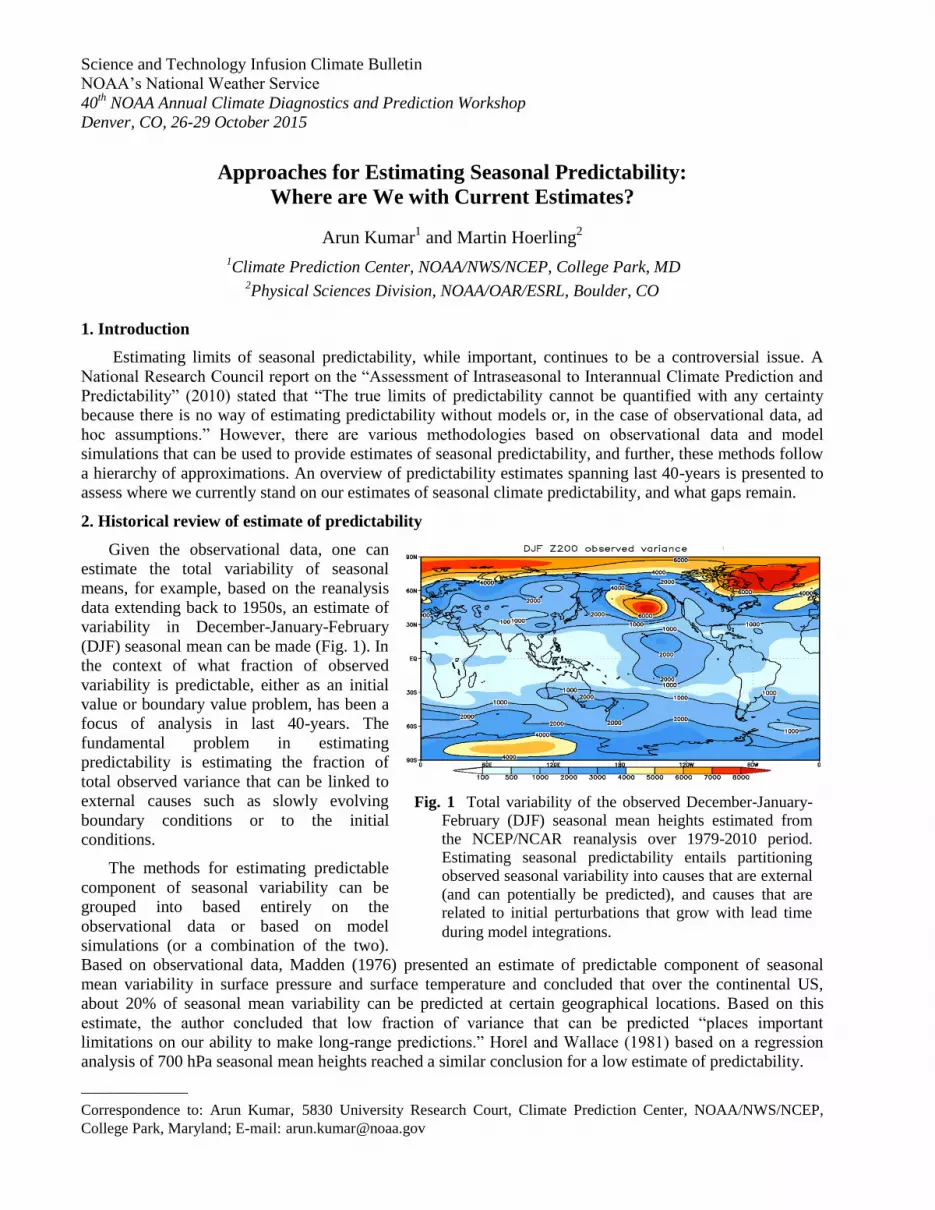
Science and Technology Infusion Climate Bulletin
NOAA’s National Weather Service
40th NOAA Annual Climate Diagnostics and Prediction Workshop
Denver, CO, 26-29 October 2015
______________
Correspondence to: Arun Kumar, 5830 University Research Court, Climate Prediction Center, NOAA/NWS/NCEP,
College Park, Maryland; E-mail: [email protected]
Approaches for Estimating Seasonal Predictability:
Where are We with Current Estimates?
Arun Kumar1 and Martin Hoerling
2
1Climate Prediction Center, NOAA/NWS/NCEP, College Park, MD 2Physical Sciences Division, NOAA/OAR/ESRL, Boulder, CO
1. Introduction
Estimating limits of seasonal predictability, while important, continues to be a controversial issue. A
National Research Council report on the “Assessment of Intraseasonal to Interannual Climate Prediction and
Predictability” (2010) stated that “The true limits of predictability cannot be quantified with any certainty
because there is no way of estimating predictability without models or, in the case of observational data, ad
hoc assumptions.” However, there are various methodologies based on observational data and model
simulations that can be used to provide estimates of seasonal predictability, and further, these methods follow
a hierarchy of approximations. An overview of predictability estimates spanning last 40-years is presented to
assess where we currently stand on our estimates of seasonal climate predictability, and what gaps remain.
2. Historical review of estimate of predictability
Given the observational data, one can
estimate the total variability of seasonal
means, for example, based on the reanalysis
data extending back to 1950s, an estimate of
variability in December-January-February
(DJF) seasonal mean can be made (Fig. 1). In
the context of what fraction of observed
variability is predictable, either as an initial
value or boundary value problem, has been a
focus of analysis in last 40-years. The
fundamental problem in estimating
predictability is estimating the fraction of
total observed variance that can be linked to
external causes such as slowly evolving
boundary conditions or to the initial
conditions.
The methods for estimating predictable
component of seasonal variability can be
grouped into based entirely on the
observational data or based on model
simulations (or a combination of the two).
Based on observational data, Madden (1976) presented an estimate of predictable component of seasonal
mean variability in surface pressure and surface temperature and concluded that over the continental US,
about 20% of seasonal mean variability can be predicted at certain geographical locations. Based on this
estimate, the author concluded that low fraction of variance that can be predicted “places important
limitations on our ability to make long-range predictions.” Horel and Wallace (1981) based on a regression
analysis of 700 hPa seasonal mean heights reached a similar conclusion for a low estimate of predictability.
Fig. 1 Total variability of the observed December-January-
February (DJF) seasonal mean heights estimated from
the NCEP/NCAR reanalysis over 1979-2010 period.
Estimating seasonal predictability entails partitioning
observed seasonal variability into causes that are external
(and can potentially be predicted), and causes that are
related to initial perturbations that grow with lead time
during model integrations.

KUMAR AND HOERLING
109
Robust estimates of seasonal
predictability can be made from
ensemble of model simulations and
initialized predictions. The basic
premise of model based estimates is
based on the assumption that among an
ensemble of simulations the common
variability (defined as the variability of
ensemble mean) is the predictable
component of seasonal variability while
the variability different from ensemble
mean is the unpredictable component.
One of the earliest model estimates of
seasonal mean predictability of
wintertime 200 hPa heights was made
by Kumar and Hoerling (1995), and the
results were consistent with the
estimates of low predictability of
Madden (1976) and Horel and Wallace
(1981) in extratropical latitudes. Kumar
and Hoerling (1995) also demonstrated
that the predictability was largest in the
tropical latitudes (and was associated
with interannual variability of sea
surface temperatures), and decreased
monotonically in extratropical latitudes.
The predictability estimate of Kumar and Hoerling (1995) was based on the analysis of a single model
and which could be erroneous due to model biases. To rectify this issue, Kumar et al. (2007) presented an
analysis based on simulations from multiple models. More recently this estimate based on this approach was
updated based on initialized forecasts from the North American Multi-Model Ensemble (NMME) (Kirtman et
al. 2014). The latest estimate of predictability (Fig. 2) still corroborate results from Madden (1976) and Horel
and Wallace (1981) in that the predictability in the extratropical latitudes is only a small fraction of total
variability. These results are consistent with the low skill of seasonal predictions in extratropical latitudes
(Peng et al. 2012).
3. Summary
Over last 40 years, vigorous research efforts have gone into estimating the predictable component of the
observed seasonal variability. These estimates are based on observational data and ensemble of model
simulations. Further, different methods rely on different level of sophistication with estimates based on
methods ranging from linear to non-linear procedures. Irrespective to the methodologies used, however, the
general conclusions have remained quite robust – largest predictability in seasonal means is in tropical
latitudes and decreases monotonically towards the extratropical latitudes; a large fraction of variability in
extratropical latitudes, consistent with the growth of initial forecast perturbations, is unpredictable. A
continued update in estimates of predictability based on newer generation of seasonal forecast systems will be
useful in the validation for the current estimates of predictability.
Acknowledgements. This study was supported by NOAA's Climate Program Office's Modeling, Analysis,
Predictions, and Projections program.
References
Horel, J. D., and J. M. Wallace, 1981: Planetary-scale atmospheric phenomenon associated with the Southern
Oscillation. Mon. Wea. Rev., 109, 2080-2092.
Fig. 2 Estimate of signal-to-noise (SNR) ratio for December-
January-February (DJF) seasonal mean heights estimated from
North American Multi-Model Ensemble (NMME). SNR is the
ratio of predictable and unpredictable component of the total
seasonal variability. Larger (smaller) values of SNR indicate
higher (lower) predictability. Predictability is higher (lower) in
tropical (extratropical) latitudes.

SCIENCE AND TECHNOLOGY INFUSION CLIMATE BULLETIN
110
Jha, B., A. Kumar, and Z.-Z. Hu, 2016: An update on the estimate of predictability of seasonal mean
atmospheric variability using North American Multi-Model Ensemble. Climate Dynamics. Submitted.
Kirtman, B. P., and co-authors, 2014: The North American Multimodel Ensemble: Phase 1 seasonal-to-
interannual prediction; Phase-2 toward developing intraseasoanl prediction. Bull. Amer. Meteor. Soc., 95,
585-601.
Kumar, A., and M. P. Hoerling, 1995: Prospects 337 and limitation of seasonal atmospheric GCM predictions.
Bull. Amer. Metor. Soc., 76, 335-345.
Kumar, A., B. Jha, Q. Zhang, and L. Bounoua, 2007: A new methodology for estimating the unpredictable
component of seasonal atmospheric variability. J. Climate, 20, 3888-3901.
Madden, R. A., 1976: Estimates of the natural variability of time-averaged sea-level pressure. Mon. Wea. Rev.,
104, 942-952.
National Research Council, 2010: Assessment of Intraseasonal to Interannual Climate Prediction and
Predictability, 192 PP., ISBN-10: 0-309-15183-X, National Academies Press, Washington, D. C., USA.
Peng, P., A. Kumar, M. S. Halpert, and A. Barnston, 2012: An analysis of CPC’s operational 0.5 month lead
seasonal outlooks. Weather and Forecasting, 27, 898-917.

Science and Technology Infusion Climate Bulletin NOAA’s National Weather Service 40th NOAA Annual Climate Diagnostics and Prediction Workshop Denver, CO, 26-29 October 2015
______________
Correspondence to: Yan Xue, 5830 University Research Court, Climate Prediction Center, NOAA/NWS/NCEP, College Park, Maryland; E-mail: [email protected].
A Real-time Multiple Ocean Reanalyses Intercomparison Project for Quantifying the Impacts of Tropical Pacific Observing Systems on Constraining Ocean Reanalyses and Enhancing our Capability in
Monitoring and Predicting ENSO
Y. Xue1, C. Wen1, A. Kumar1, M. Balmaseda2, Y. Fujii3, G. Vecchi4, G. Vernieres5, O. Alves6, M. Martin9, F. Hernandez10, T. Lee7, D. Legler8, and D. DeWitt1
1Climate Prediction Center, NOAA/NWS/NCEP, College Park, Maryland, USA 2European Center for Medium-Range Weather Forecasts, Reading, UK
3Japan Meteorological Agency, Tokyo, Japan 4Geophysical Fluid Dynamics Laboratory, NOAA/OAR, Princeton, NJ, USA
5Goddard Space Flight Center, NASA, Greenbelt, MD, USA 6Bureau of Meteorology, Melbourne, Australia
7Jet Propulsion Laboratory, NASA, Pasadena, CA, USA 8Climate Program Office, NOAA, Silver Spring, MD, USA
9UK Met Office, Exeter, Devon, United Kingdom 10Mercator Ocean, France
ABSTRACT
To quantify uncertainties in the current generation of ocean reanalysis products, CLIVAR Global Synthesis and Observations Panel (GSOP) and the GODAE OceanView (GOV) jointly initiated Ocean Reanalysis (ORA) Intercomparison Project (ORA-IP). For those ocean reanalyses produced by operational centers for initialization of climate models or short-range ocean forecast models, there is an opportunity to conduct ORA intercomparison in near real-time, and to use the ensemble approach to quantify the signal (ensemble mean) and noise (ensemble spread) in our estimation of ocean climate variability. Motivated by the Tropical Pacific Observing System (TPOS) 2020 Workshop held in January 2014 in La Jolla, CA, with support from NOAA Climate Observation Division, the CPC initiated and led a Real-Time ORA-IP. An ensemble of nine operational ORAs is been routinely collected, and they are used to monitor consistency and discrepancy in the tropical Pacific temperature analysis in real time in support of ENSO monitoring and prediction.
The role of the TAO/TRITON buoy data on constraining the ocean reanalyses is assessed by root-mean-square error (RMSE) and anomaly correlation (AC) with the buoy temperature data directly. The ensemble mean is shown to have a higher accuracy (smaller RMSE and larger AC) than individual product, suggesting the ensemble approach is an effective tool in reducing uncertainties in temperature analysis for ENSO. The spread among the ensemble mean and its time variability measures how uncertainties vary with location and time. The temporal variability of the spread can be partially linked to the temporal variability of in situ observations which reduce ocean analysis errors and increase consistency among them. The important outcomes of the project are to 1) provide estimation where uncertainties are large and if sustained or enhanced ocean observations are needed to reduce uncertainties, 2) to provide the most reliable estimate of climate signal such as ENSO, and 3) to provide the signal to noise ratio for the climate signal in real time.

SCIENCE AND TECHNOLOGY INFUSION CLIMATE BULLETIN
112
1 Introduction
Ocean reanalyses (ORAs) aim to provide an optimal estimation of 3-dimensional structures of the ocean by combining model solutions with ocean observations via data assimilation methods. However, the time evolution represented by an ORA will be sensitive to the temporal variations of the observing system, to the errors of the ocean model, atmospheric fluxes and assimilation systems, which are often flow-dependent, and not easy to estimate. A crude and pragmatic way of estimating uncertainties in ORAs is to carry out an intercomparison of ORAs within the framework of an ensemble approach.
The multi-analysis ensemble approach is adopted by the Ocean Reanalyses Intercomparison Project (ORA-IP) jointly coordinated by the CLIVAR Global Synthesis and Observation Panel (GSOP) and GODAE OceanView (Balmaseda et al. 2015). Some ORAs in the ORA-IP are continuously updated in real-time in operational centers for initialization of seasonal forecast models or short-range ocean forecast models. Those real-time ORAs, often referred to as operational ORAs, have the additional advantage that they allow monitoring of climate variability such as El Niño/Southern Oscillation (ENSO) and those beyond ENSO (Xue et al. 2010). The operational ORAs are now routinely used at national climate centers for ENSO monitoring, and prediction efforts.
The quality of the ORAs for monitoring ENSO depends critically on the Tropical Pacific Observing Systems (TPOS), which was initially populated by the Tropical Atmospheric Ocean (TAO) array in early-1980s (McPhaden et al. 1998), and was later enhanced by the Triangle Trans-Ocean Buoy Network (TRITON) array in the western tropical Pacific (west of 160˚E) after 2000 (Ando et al., 2005). The TAO/TRITON array is considered as the cornerstone of the ENSO observing system, as it systematically measures upper ocean temperature, current and air-sea fluxes etc. at geographically fixed locations. The implementation of the TAO/TRITON array stimulated a rapid development of operational ocean reanalyses (e.g. Behringer et al. 1998; Alves et al. 2004; Zhang et al. 2007; Yin et al. 2011; Balmaseda et al. 2013).
Product Forcing Configuration Data Assim. Method
Analysis Period
GFDL/NOAA (ECDA) Coupled DA 1ox1/3° MOM4 coupled EnKF (T/S/SST) 1979-present
GMAO/NASA (MERRA Ocean) Merra + Bulk 0.5° MOM4 EnOI (SLA/T/S/SST/SIC) 1979-present
NCEP/NOAA (GODAS) NCEP-R2 Flux. 1°x1/3° MOM3 3DVAR (SST/T) 1979-present
NCEP/NOAA (CFSR) Coupled DA 0.5°x1/4° 3DVAR (SST/T) 1979-present
CAWCR/BOM
(PEODAS) ERA40 to 2002; NCEP-R2
thereafter. Flux 1°x2° MOM2 EnKF (T/S/SST) 1979-present
ECMWF
(ORAS4) ERA40 to 1988; ERAi
thereafter. Flux. 1°x 1/3° NEMO3 3DVAR (SLA/T/S/SST) 1979-present
MRI/JMA
(MOVE-G2) JRA-55 corr+ CORE Bulk 1ox0.5° MRI.COM3 3DVAR (SLA/T/S/SST) 1979-present
UK MET (GloSea5) ERAi+CORE Bulk 1/4° NEMO3.2 3DVAR
(SLA/T/S/SST/SIC) 1993-present
MERCATOR (GLORYS2V3) ERAi corr+ CORE Bulk 1/4° NEMO3.1 EnKF+3DVAR
(SLA/T/S/SST/SIC) 1993-present
§Table 1 List of ocean reanalysis products entering the inter-comparison.
§ The data assimilation column lists the observation types used for their estimation (T/S for temperature and salinity; SLA: altimeter-derived sea level anomalies; SST: sea surface temperature, SIC: sea-ice concentration), as well as assimilation techniques used for reanalysis: Ensemble Optimal Interpolation (EnOI), Ensemble Kalman Filter (EnKF), variational methods (3D-Var). The atmospheric surface forcing is usually provided by atmospheric reanalyses, using either direct daily fluxes, or different bulk formulations. There are also systems that use fluxes from coupled data assimilation systems (Coupled DA), which come in multiple flavours (parameter estimation, EnKF, weakly coupled).

XUE ET AL.
113
The rapid decline of the TAO array after summer 2012 and anticipating substantial reduction in the TRITON array in next few years raised a serious concern among the ocean data assimilation community if the quality of the operational ORAs has been compromised due to the data loss. One of the recommendations from the TPOS 2020 workshop (http://www.ioc-goos.org/tpos2020) is to monitor the consistency and discrepancy across the operational ORAs in real time to support ENSO forecast, and to monitor the impacts of the TAO/TRITON data loss on the quality of ORAs (Fujii et al. 2015).
With the support from NOAA Climate Observation Division, the Climate Prediction Center (CPC) of National Centers for Environmental Prediction (NCEP) initiated and led the Real-Time ORA-IP following the TPOS 2020 Workshop. An ensemble of nine operational ORAs (Table 1) is been routinely collected, and an experimental web site has been constructed to display the ensemble ORA products with a focus on monitoring the consistency and discrepancy in tropical Pacific temperature analyses in real time in support of ENSO monitoring and prediction (http://www.cpc.ncep.noaa.gov/products/GODAS/multiora_body.html for the 1981-2010 climatology; http://www.cpc.ncep.noaa.gov/products/GODAS/multiora93_body.html for the 1993-2013 climatology that is partially finished). The objectives of the project are to 1) provide estimation where uncertainties among operational ORAs are largest and if sustained or enhanced ocean observations are needed to reduce uncertainties, 2) to provide the most reliable estimate of climate signal such as ENSO, and 3) to provide the signal to noise ratio for climate signal in real time.
2 Results
2.1 Comparison with the TAO/TRITON data
In the tropical Pacific, in addition to assimilating the TAO/TRITON data, ORAs also assimilate temperature and salinity observations from the Argo floats and expendable bathythermographs (XBTs). It is important to know how well each ORA fits to the TAO/TRITON data. The temperature observations from 66 buoys that have more than 10 year record of monthly values are included in the comparison. The buoy data are linearly interpolated onto the same vertical grid (with 10m interval) as that in the ORAs. For the comparison, each ORA is sampled identically in time as the buoy data and temperature anomalies are constructed by removing the climatology for each ORA and buoy data separately. The root-mean-square error (RMSE) and anomaly correlation (AC) are then calculated at each level for every buoy site. Normalized RMSE (NRMSE) is calculated as the RMSE divided by the standard deviation (STD) of TAO temperature anomalies at each level for every buoy site. To get an integrated measurement of the fit to the buoy data, RMSE, NRMSE and AC are averaged at all levels in the upper 300m.
Table 2 shows the averaged RMSE and NRMSE over the upper 300m in five regions. The NRMSE of each ORA is compared with that of the ensemble mean (EM), defined as the average of the nine ORAs, which
RMSE of EM (
oC) NRMSE of
EM (%)
NRMSE Difference from EM (%) NCEP
GODAS JMA ECMWF GFDL NASA BOM
UK MET
MERCATOR NCEP CFSR
EEPac 0.26 21 7 10 5 14 13 7 -3 9 19 WEPac 0.25 24 8 11 4 19 10 8 1 14 17 NEPac 0.33 38 15 14 2 17 27 16 -11 6 24 NWPac 0.29 27 7 11 0 20 13 19 -4 10 20
SPac 0.21 24 3 7 3 27 12 10 -2 11 23
Table 2 Root-mean-square error (RMSE, the second column) and normalized RMSE (NRMSE, the third column) of temperature anomaly from TAO observations averaged in upper 300m in 1993-2014 for the ensemble mean (EM). NRMSE is RMSE divided by standard deviation (STD) of TAO temperature anomalies expressed as percentage (%). Positive (negative) difference of NRMSE of each ORA from EM (the 4th-11th column) indicates increased (decreased) NRMSE from that of EM (values higher than 15% are in bold). Shown are the values calculated for each TAO/TRITON buoy and averaged in the eastern equatorial Pacific (170oW-90oW, 2oS/0/2oN, EEPac), the western equatorial Pacific (120oE-180oW, 2oS/0/2oN, WEPac), the northeastern subtropical Pacific (170oW-90oW, 5oN/8oN, NEPac), the northwestern subtropical Pacific (120oE-180oW, 5oN/8oN, NWPac), and the southern subtropical Pacific (120oE-90oW, 5oS/8oS, SPac).

SCIENCE AND TECHNOLOGY INFUSION CLIMATE BULLETIN
114
is expected to have the smallest RMSE. For the eastern equatorial Pacific (EEPac), the RMSE of EM is 0.26oC and NRMSE is about 21% of STD. Individual ORA tends to have larger NRMSE (5-19% STD) except the MET. This is consistent with the wisdom that the ensemble mean tends to cancel out noises in individual ORA and to provide a better analysis than individual ORA. In the western equatorial Pacific (WEPac), the RMSE and NRMSE are similar to those in EEPac and the EM is generally superior to individual ORA. In the northeastern Pacific (NEPac), the RMSE (0.33oC) and NRMSE (38%) are considerably higher than those in other regions. Compared to the EM, individual ORA has higher NRMSE except the MET which has smaller NRMSE. For the northwestern Pacific (NWPac) and southern Pacific (SPac), the conclusion is similar to the above. Individual ORA tends to have larger NRMSE than the EM except the MET. We will discuss next why the MET fits to the buoy data much better than other ORAs. If the NRMSE in the five regions is averaged, the ORAs ranked from the lowest to highest NRMSE are MET, ECMWF, NCEP GODAS, MERCATOR, JMA, BOM, NASA, GFDL and NCEP CFSR. We will explain in next section that the better fit to the buoy data at limited buoy sites may not represent a better analysis when all the grid points are considered.
2.2 Comparison with the ensemble mean
It is shown earlier that the ensemble mean (EM) tends to be superior to individual ORA in the fit to the TAO/TRITION data. Another advantage of the EM is that it has a uniform coverage of all grid points and provides us the best estimation of climate signal in locations where not covered by the isolated mooring sites.
Fig. 1 Root-mean-square error (RMSE) of temperature anomaly for (a) NCEP_GODAS, (b) ECMWF, (c) JMA, (d) GFDL, (e) NASA, (f) BOM, (g) MET, (h) MERCATOR, and (i) NCEP_CFSR computed against the ensemble mean and averaged in upper 300m. The RMSE is computed over 1993-2014. Unit is oC.

XUE ET AL.
115
In the ensemble approach, the true signal in the ocean state is estimated as the ensemble mean (EM) based on all ORAs
(1)
where denotes an individual ORA and N is the total number of ORAs. The root-mean-square error (RMSE) relative to the EM measures how well each ORA agrees with the EM. Fig. 1 shows that the RMSE is generally small (< 0.3oC) in the equatorial belt where TAO observations help constrain the analysis. A noticeable exception is larger values in the MET west of 180oE, and in locations between the mooring sites. Another exception is larger values in the CFSR (> 0.4oC) east of 150oW and in the GFDL west of 150oE. The RMSE is much larger in the off-equatorial belt, and the MET, the NCEP_GODAS and NCEP_CFSR, along with the GFDL product, stand out as the ones with the largest RMSE.
The RMSE at the equator (Fig. 2) shows that the largest error is located near the mean thermocline. The UK MET and the two NCEP reanalyses have the largest departure from the EM. The large RMSE in the UK MET is largely due to a too strong fit to observations in the presence of large model biases. The large RMSE in the NCEP CFSR can be partially attributed to a sudden shift in climatology near 1999 (Xue et al. 2011), and for the GODAS is largely due to the warm biases before 1990.
Fig. 2 Root-mean-square error (RMSE) of temperature anomaly at the equator for (a) NCEP_GODAS, (b) ECMWF, (c) JMA, (d) GFDL, (e) NASA, (f) BOM, (g) MET, (h) MERCATOR, and (i) NCEP_CFSR computed against the ensemble mean. The RMSE is computed over 1993-2014. Unit is oC.

SCIENCE AND TECHNOLOGY INFUSION CLIMATE BULLETIN
116
2.3 Uncertainties among ocean reanalyses
The uncertainty in the ocean state estimation can be quantified by the spread of ocean reanalyses from the ensemble mean
(2)
(3)
where M is the number of samples in the time series.
To see how temporal variations in ocean observations contribute to reduce Fig.3 shows the and the corresponding data counts during the period
a) prior to the completion of TAO array (1985 to 1993), b) after the completion of TAO array but prior to the ARGO (1994 to 2003), and c) 2004 to 2011 after the full deployment of TAO/TRITON and ARGO.
The full deployment of the TAO array significantly reduces the analysis uncertainty in the equatorial Pacific, and the availability of Argo reduces the analysis uncertainty in off-equatorial regions, thus clearly highlight the positive influence of ocean observations on constraining the ocean analysis. However, there is still large spread in the northwestern tropical Pacific, in the SPCZ region and central and northeastern tropical Pacific. Fig. 3 also indicates that the data assimilation systems tend to constrain the solution very locally, only where there are in situ observations. This suggests that enhancing ocean observing systems should go hand in hand with improving ocean data assimilation systems such that ocean observations can be optimally utilized by those systems.
Considering the significant loss of the TAO data in the equatorial eastern Pacific in 2012-13, we examined the temporal variations of the spread in the equatorial eastern Pacific (EEPac), and related it to the temporal variability of signal and data counts. Fig. 4 shows that the spread is relatively large before 1990 when where was little data, and stays relatively low from 1990 to 2005 except during the 1982/83 and 1997/98 El Nino. However, there is a gradual increase of the spread after 2005 and a noticeable peak in 2012-2013 when there was a significant loss of the TAO data.
3 Summary and discussions
Since the inception of this project at CPC in 2014, major accomplishments include:
• Establishing protocols for routine collection of ocean reanalyses from different operational centers;
• A web page to display ocean reanalyses
Fig. 3 (Left column) The ensemble spread of temperature anomaly averaged in the upper 300m in (a) from 1985 to 1993, (b) from 1994 to 2003, and (c) from 2004 to 2011, along with (right column) the associated data counts (number of daily temperature profiles in each 1x1 degree box).

XUE ET AL.
117
and uncertainty among them; • An ability to provide a sanity
check for potential issues among various ocean reanalyses;
• A demonstration of possible issues with NCEP ocean reanalyses systems, i.e., GODAS and CFSR;
• Evidence for the influence of temporal variations in situ data on the uncertainty among ocean reanalyses, viz a reduction in in situ data leading to an increase in analysis uncertainty.
As the data delivery from external centers is now mostly routine, we plan to devote additional time in better quantification of the impacts of evolution of TPOS on the ocean analysis and uncertainty among them. In future, results from this project will
a) provide support for the framework of TPOS 2020 (http://tpos2020.org/) project on the design of the future tropical Pacific observing system;
b) continue to deliver real-time information to the user community with stake in ENSO monitoring and prediction, and
c) support a comprehensive assessment of the next generation of ocean reanalysis at NCEP.
References
Alves, O., M. Balmaseda, D. Anderson, and T. Stockdale, 2004: Sensitivity of dynamical seasonal forecasts to ocean initial conditions. Q. J. R. Meteorol. Soc., 130, 647– 668.
Ando, K., T. Matsumoto, T. Nagahama, I. Ueki, Y. Takatsuki, and Y. Kuroda, 2005: Drift characteristics of a moored conductive-temperaturedepth sensor and correction salinity data. J. Atmos. Ocean. Technol., 22, 282–291. doi:10.1175/JTECH1704.1
Balmaseda, M.A., and K. Mogensen, A.T. Weaver, 2013: Evaluation of the ECMWF ocean reanalysis system ORAS4. Q. J. R. Meteorol. Soc., 131, 1132-1161.
Balmaseda, M, and Coauthors, 2015: The Ocean Reanalyses Intercomparison Project (ORA-IP). J. Oper. Oceanogr., 7, 81–99.
Behringer, D.W., M. Ji, and A. Leetmaa, 1998: An improved coupled model for ENSO prediction and implications for ocean initialization. Part I: The ocean data assimilation system. Mon. Wea. Rev., 126, 1013-1021.
Fujii, Yosuke, J. Cummings, Y. Xue, A. Schiller, T. Lee, M. A. Balmaseda, E. Rémy, S. Masuda, G. Brassington, O. Alves, B. Cornuelle, M. Martin, P. Oke, G. Smith and X. Yang, 2015: Evaluation of the
Fig. 4 (top panel) The number of daily temperature profiles from TAO/TRITON (red line), TAO/TRITON/Argo/XBT (blue line), (middle panel) the standard deviation of temperature anomaly of the ensemble mean of seven products (solid line) and nine products (dash line), and (bottom panel) the ensemble spread averaged in the upper 300m based on seven products (solid line) and nine products (dash line) for the eastern equatorial Pacific (EEPac, 160oW-90oW, 2oS-2oN).

SCIENCE AND TECHNOLOGY INFUSION CLIMATE BULLETIN
118
Tropical Pacific Observing System from the Ocean Data Assimilation Perspective. Q. J. R. Meteorol. Soc., 141, 2481-2496. doi:10.1002/qj.2579.
McPhaden, M.J., and Coauthors, 1998: The tropical ocean–global atmosphere (TOGA) observing system: a decade of progress. J. Geophys. Res., 103, 14,169–14,240.
Xue, Y., B. Huang, Z.-Z. Hu, A. Kumar, C. Wen, D.W. Behringer, and S. Nadiga, 2011: An assessment of oceanic variability in the NCEP Climate Forecast System Reanalysis. Clim. Dyn., 37, 2511–2539. doi:10.1007/s00382-010-0954-4
—, and Coauthors, 2010: Ocean state estimation for global ocean monitoring: ENSO and beyond ENSO. Proceedings of ocean obs’09: sustained ocean observations and information for society (vol. 2). Venice, Italy, 21–25 September 2009, J. Hall, D.E. Harrison, and D. Stammer, Ed., ESA Publication WPP-306.
Yin, Y., O. Alves, and P. Oke, 2011: An ensemble ocean data assimilation system for seasonal prediction. Mon. Wea. Rev., 139, 786–808. doi: http://dx.doi.org/10.1175/2010MWR3419.1
Zhang, S., M.J. Harrison, A. Rosati, and A. Wittenberg, 2007: System design and evaluation of coupled ensemble data assimilation for global oceanic studies. Mon. Wea. Rev., 135, 3541–3564.

6. PREDICTION / ATTRIBUTIONOF ARCTIC CLIMATEVARIABILITY AND LINKAGESTO LOWER LATITUDES
40th NOAA Climate Diagnostics and Prediction Workshop

Science and Technology Infusion Climate Bulletin NOAA’s National Weather Service 40th NOAA Annual Climate Diagnostics and Prediction Workshop Denver, CO, 26-29 October 2015
______________
Correspondence to: Thomas W. Collow, 5830 University Research Court, INNOVIM, LLC| NOAA/NWS/NCEP Climate Prediction Center, College Park, MD; E-mail: [email protected].
Prediction of Arctic Sea Ice Melt Date as an Alternative Parameter for Local Sea Ice Forecasting
Thomas W. Collow1,2, Wanqiu Wang2, and Arun Kumar2 1INNOVIM, LLC, Greenbelt, MD
2Climate Prediction Center, NOAA/NWS/NCEP, College Park, MD
1. Introduction
Accurate seasonal prediction of Arctic sea ice is an essential need for stakeholders in that region. However, current commonly used metrics of sea ice extent or sea ice area, which provide an integrated total over the entire Arctic, are of limited use to those who seek information on a more local scale. Shipping operations in the Arctic are concerned with the sea ice melt in the summer which impacts transportation routes. As Arctic warming continues, a greater region will experience melt, which will lead to a thinner winter ice pack. More frequent melting will also enhance the Arctic albedo feedback leading to additional warming and thus more melting (Stroeve et al. 2011 and references within). Therefore, an accurate prediction of sea ice melt on a local scale will prove valuable for a variety of Arctic initiatives.
Previous studies have examined passive microwave satellite data to determine the observed first sea ice melt day (IMD) (Smith 1998; Kwok et al. 2003; Belchansky et al. 2004; Howell et al. 2009; Markus et al. 2009; Stroeve et al. 2014; and others). Observed trends generally show earlier ice melt dates. Specifically Markus et al. (2009) and Stroeve et al. (2014) show mean trends in IMD of -2.5 and -1.9 days/decade respectively across the Arctic. The goal of this work is to analyze the performance of the Climate Forecast System version 2 (CFSv2, Saha et al. 2014) in representing IMD using both the operational settings and an experimental configuration.
2. Data and methods
Modeled sea ice concentration data from CFSv2 hindcasts are used. Two model configurations are used, the operational setting (CFSv2CFSR) which uses initial conditions from the Climate Forecast System Reanalysis (CFSR, Saha et al. 2010), and an experimental version (CFSv2PIOMp) used in Collow et al. (2015). CFSv2PIOMp proved to be more representative of the downward trend in sea ice during later years than CFSv2CFSR. For CFSv2PIOMp, the model was initialized with sea ice thickness from the Pan-Arctic Ice Ocean Modeling and Assimilation System (Zhang and Rothrock 2003) and additional modifications were made to the internal physics settings. Observed data used are the NASA Team sea ice concentrations from Nimbus-7 SMMR and DMSP SSM/I (available at ftp://sidads.colorado.edu/DATASETS). Observations were studied from 1985-2014 to get a sense of changes in the last 30 years. Model runs were then initialized 8-12 March 00 UTC 2005-2014 and run through 31 December for a total of 50 simulations for each model configuration, five for each year. The melt season from 1 April through 30 September is analyzed and compared with observations from this period to assess model performance.
CFSv2 sea ice concentrations are output at 12-hour intervals. Therefore, these are interpolated to match the daily frequency of the NASA Team data by averaging the two model data time steps on each day. NASA Team data prior to August 1987, which is available every other day, is linearly interpolated to a daily resolution. For all years, IMD is determined as the first day sea ice concentration drops below 15% after 1 April following the traditional definition of sea ice extent from the Intergovernmental Panel on Climate Change assessment report (Vaughan et al. 2013). Points that never cross the 15% threshold (permanently frozen or permanently melted) are set to undefined, thereby limiting data to seasonal sea ice regions only. Means are determined for modeled and observed IMD for each grid point. For modeled data, IMD from each of the 5 ensembles is averaged to determine the mean for that year to compare to observations.

COLLOW ET AL.
121
3. Comparison of modeled and observed means
First observed NASA Team IMD means are compared over two different time periods, 1985-1994 and 2005-2014. As seen in Figure 1b, the later period has a more expansive region of ice melt over the Arctic Ocean than in the early period (Figure 1a). Differences (Figure 1c) show generally earlier ice melt days throughout the entire Arctic. Using a t-test, significant differences at 95% confidence are found over the Hudson Bay, Davis Strait, Barents Sea, and somewhat over the Chukchi Sea. There are some regions which experienced later melt in 2005-2014 than in 1985-1994, specifically in the Bering Strait and the East Siberian Sea but changes in these regions do not show significance.
Fig. 1 Mean of observed IMD from NASA Team for the 1985-1994 period (a) and the 2005-2014 period (b). Difference between the two (b minus a) is shown in c. Hatching in c denotes differences are significant at 95% confidence based on a t-test.
Fig. 2 Mean 2005-2014 IMD from CFSv2CFSR (a) and CFSv2PIOMp (b); CFSv2CFSR bias with respect to NASA Team observations (c); CFSv2PIOMp bias with respect to NASA Team observations (d); Difference between CFSv2PIOMp and CFSv2CFSR (e); mean absolute error difference between CFSv2PIOMp and CFSv2CFSR (abs[CFSv2PIOMp-NASA] minus abs[CFSv2CFSR-NASA]) (f.).

SCIENCE AND TECHNOLOGY INFUSION CLIMATE BULLETIN
122
Using CFSv2 hindcasts to compare with the observations during the 2005-2014 period, it is evident from Figure 2 that CFSv2PIOMp has more extensive sea ice melt (Figure 2b) than CFSv2CFSR (Figure 2a) in the Arctic which is in line with the observations for this period. Differences with respect to the observations show that positive biases in the modeled IMD are smaller for CFSv2PIOMp (Figure 2d) than CFSv2CFSR (Figure 2c). However, both model configurations show ice melt occurring too early over the Bering Strait. Across the Arctic Ocean and Barents Sea, CFSv2PIOMp has a significantly earlier IMD than CFSv2CFSR (Figure 2e). There is a significant increase in IMD over southern Hudson Bay. Improvements in the prediction of IMD from each model configuration were determined using mean absolute error differences and it was found that CFSv2PIOMp significantly improved IMD prediction over the Barents Sea and a small part of the Chukchi Sea (Figure 2f). However, the skill using CFSv2PIOMp was degraded over southern Hudson Bay. One caveat is that taking differences only accounts for points that appear in both datasets or are common to the two time periods, which will not quantify differences over places with new melt over the last decade such as the interior Arctic Ocean. Changes in this region are addressed in the next section.
Fig. 3 Histogram showing the mean area of sea ice melt for each day of the year over the Arctic Ocean (a, b) and Hudson Bay (c, d); Panels a and c show the mean distribution for the NASA Team data for 1985-1994 (dashed line) and 2005-2014 (solid line); Panels b and d show the mean distribution for the CFSv2 2005-2014 hindcasts for CFSv2CFSR (blue line) and CFSv2PIOMp (red line). A 15-day smoothing was applied to all lines.

COLLOW ET AL.
123
4. Distribution over the Arctic Ocean and Hudson Bay
Looking at the mean distribution of IMD over the Arctic Ocean, it is apparent that there has been a substantial increase in the area of the observed melt region in the 2005-2014 period over the 1985-1994 period (Figure 3a). CFSv2PIOMp shows the large area of melt in the Arctic Ocean but CFSv2CFSR fails to do so (Figure 3b) highlighting that the experimental modeling system is superior for this region. The peak melt days for the NASA Team observations for 1985-1994 and 2005-2014 are 207 and 209 respectively indicating little change in the timing of melt. The peak melt day in the models is also very similar (206 for CFSv2CFSR and 207 for CFSv2PIOMp) indicating that the issue is not necessarily in the temporal cycle of sea ice melt, but in the magnitude. Similar distribution plots are also shown for Hudson Bay. There is a noticeable shift in the observed distribution toward an earlier peak melt (Figure 3c, peak melt was 192 in the 1995-2004 in the early period and 178 in the 2005-2014 period). However, as previously shown in the last section, CFSv2PIOMp was not as skillful in this region and it is reflected in Figure 3d. For CFSv2CFSR the peak melt day for the 2005-2014 period was 177, closely matching the observed. For CFSv2PIOMp this increased to 183, which is actually further from the observed.
5. Summary and conclusions
The largest observed changes in IMD between the 1985-1994 and 2005-2014 periods occur over select regions of the Arctic, namely the Hudson Bay, Davis Strait, Barents Sea, and the Arctic Ocean. The operational system (CFSv2CFSR) does not capture early melting over the Arctic Ocean and Barents Sea but performs better over the Hudson Bay. Conversely the experimental set-up (CFSv2PIOMp) improves prediction over the Arctic Ocean and Barents Sea but degrades the prediction slightly over Hudson Bay. The improvements in the Arctic Ocean are mostly seen in the distribution, not direct differences, where there are only a small number of common IMD points between the two periods. The more realistic melting in the Arctic Ocean in CFSv2PIOMp is likely attributed to a better representation of initial sea ice thickness, which is covered in detail in Collow et al. (2015). Overall, exact IMD dates are hard to predict, primarily due to issues in model resolution and atmospheric influences that cannot possibly be predicted months in advance. However, by removing model biases and quantifying spread, it is possible to issue forecasts of IMD which can be used by stakeholders for decision making.
Work is ongoing in extending CFSv2 hindcasts back through 1980 to compare modeled and observed trends in not only IMD, but also the first ice freeze date and the melt season length.
References
Belchansky, G. I., D. C. Douglas, and N. G. Platonov, 2004: Duration of the Arctic sea ice melt season: regional and interannual variability, 1979-2001. J. Climate, 17, 67-80, doi:10.1075/1520-0442(2004)017<0067:DOTASI>2.0.CO;2.
Collow, T. W., W. Wang, A. Kumar, and J. Zhang, 2015: Improving Arctic sea ice prediction using PIOMAS initial sea ice thickness in a coupled ocean-atmosphere model. Mon. Wea. Rev., 143, 4618-4630, doi:10.1175/MWR-D-15-0097.1.
Howell, S. E. L., C. R. Duguay, and T. Markus, 2009: Sea ice conditions and melt season duration variability within the Canadian Arctic archipelago: 1979-2008. Geophys. Res. Lett., 36, L10502, doi:10.1029/2009GL037681.
Kwok, R., G. F. Cunningham, and S. V. Nghiem, 2003: A study of the onset of melt over the Arctic Ocean in RADARSAT synthetic aperture radar data. J. Geophys. Res., 108, 3363, doi:10.1029/2002JC001363.
Markus, T., J. C. Stroeve, and J. Miller, 2009: Recent changes in Arctic sea ice melt onset, freezeup, and melt season length, J. Geophys. Res., 114, C12024, doi:10.1029/2009JC005436.
Saha, S., and Coauthors, 2010: The NCEP Climate Forecast System Reanalysis, Bull. Amer. Meteor. Soc., 91, 1015-1067, doi: 10.1175/2010BAMS3001.1.
Saha, S., and Coauthors, 2014: The NCEP Climate Forecast System Version 2, J. Climate, 27, 2185-2208, doi: 10.1175/JCLI-D-12-00823.1.

SCIENCE AND TECHNOLOGY INFUSION CLIMATE BULLETIN
124
Smith, D. M., 1998: Observation of perennial Arctic sea ice melt and freeze-up using passive microwave data, J. Geophys. Res., 103, 27,753-27,769, doi:10.1029/98JC02416.
Stroeve, J. C., M. C. Serreze, M. M. Holland, J. E. Kay, J. Malanik, and A. P. Barrett, 2011: The Arctic’s rapidly shrinking sea ice cover: a research synthesis, Clim. Change, 110, 1005-1027, doi:10.1007/s10584-011-0101-1.
Stroeve, J. C., T. Markus, L. Boisvert, J. Miller, and A. Barrett, 2014: Changes in Arctic melt season and implications for sea ice loss, Geophys. Res. Lett., 41, 1216-1225, doi:10.1002/2013GL058951.
Vaughan, D. G., and Coauthors, 2013: Observations: Cryosphere, Climate Change 2013: The Physical Science Basis. Contribution of Working Group I to the Fifth Assessment Report of the Intergovernmental Panel on Climate Change, 66 pp., Cambridge University Press, Cambridge, United Kingdom and New York, NY, USA.
Zhang, J.L. and D. A. Rothrock, 2003: Modeling global sea ice with a thickness and enthalpy distribution model in generalized curvilinear coordinates, Mon. Wea. Rev., 131, 845-861.

7. TOPICS RELATED TOPREDICTABILITY AND STRATEGIES FORPREDICTION
40th NOAA Climate Diagnostics and Prediction Workshop

Science and Technology Infusion Climate Bulletin NOAA’s National Weather Service 40th NOAA Annual Climate Diagnostics and Prediction Workshop Denver, CO, 26-29 October 2015
______________
Correspondence to: Daniel S. Harnos, 5830 University Research Ct., Climate Prediction Center, NOAA/NWS/NCEP, College Park, Maryland; E-mail: [email protected]
A NMME-based Hybrid Prediction System for Atlantic Hurricane Season Activity
Daniel S. Harnos1,2, Jae-Kyung E. Schemm1, Hui Wang1 1Climate Prediction Center, NOAA/NWS/NCEP, College Park, Maryland
2Innovim LLC, Greenbelt, Maryland
A North American Multi-Model Ensemble (NMME)-based hybrid statistical-dynamical prediction system for Atlantic hurricane season tropical storm activity has been developed at Climate Prediction Center to support the NOAA Hurricane Season Outlooks. Multiple-linear regression relationships have been previously established between combinations of observed and coupled general circulation model (GCM) forecast atmospheric and oceanic states and subsequent hurricane season activity (e.g. Wang et al. 2009) and have been used in operations at the Climate Prediction Center to support NOAA’s Hurricane Seasonal Outlook. This work addresses whether aggregation of multiple GCM forecasts from the North American Multi-model Ensemble (NMME; Kirtman et al. 2014) can improve upon single GCM inputs with a similar hybrid approach.
Predictors are selected as the forecast August-October (ASO) zonal wind shear (difference between 850 and 200 hPa) over the Atlantic Main Development Region (MDR; 10-20°N, 20-80°W) and preseason sea surface temperature (SST) for the North Atlantic (55-65°N, 30-60°W) averaged over the preceding 3 months to the forecast being made. Predictands are seasonal total hurricane count, tropical storm count, major hurricane count, and accumulated cyclone energy (ACE) as a percentage of median. The prediction system was evaluated in cross-validation mode for the hindcast period of 1982-2010. Table 1 details the performance of the hybrid model predictions of seasonal hurricane count for each of the four member GCMs (CanCM3, CanCM4, CCSM4, and CFSv2) and the NMME multi-model mean in terms of correlation and root mean squared error. The NMME multi-model mean correlations exceed those of each individual member GCMs, while reducing RMSE by 19% and 25% relative to the best performing GCMs initialized in April and July respectively. Comparable relationships are also obtained for other predictands, with the NMME consistently displaying improved correlations with observed hurricane activity and reducing RMSE relative to the best
Predictand CanCM3 CanCM4 CCSM4 CFSv2 NMME Observed
Hurricanes 3 (1-5) 2 (0-3) 5 (4-6) 6 (5-7) 4 (3-5) 4
Tropical Storms 6 (1-10) 4 (1-6) 9 (8-10) 11 (9-13) 7 (5-10) 11
Major Hurricanes 1 (0-2) 1 (0-1) 2 (2-2) 2 (2-3) 1 (1-2) 2
ACE (% Median) 50 (5-94) 21 (0-45) 80 (64-96) 102 (75-128) 62 (35-91) 64%
Init. Cond. CanCM3 (10) CanCM4 (10) CCSM4 (10) CFSv2 (12) NMME (4)
April 0.42 (2.87) 0.47 (2.80) 0.46 (2.80) 0.46 (2.80) 0.49 (2.27)
July 0.67 (2.36) 0.66 (2.37) 0.62 (2.47) 0.67 (2.36) 0.71 (1.76)
Table 2: Hybrid model forecasts for April 2015 utilizing predictors of forecast ASO wind shear over the MDR and observed January-March mean North Atlantic SST. Columns indicate GCM used to force the hybrid model, with NMME referring to the multimodel mean. Last column denotes preliminary observed 2015 hurricane activity. Numbers in bold indicate the observations fell within the forecasted range.
Table 1: Hindcast ensemble mean correlations and RMSE (in parentheses) for hybrid model cross-validation with April and July initial conditions. Columns indicate GCM used to force hybrid model and number of ensemble members, with NMME referring to the multi-model mean.

HARNOS ET AL.
127
GCM member.
The hindcast evaluation indicated that the hybrid prediction system provides skillful prediction of seasonal tropical storm activity and gave impetus to attempt a real-time test for the 2015 hurricane season. For the April 2015 NMME hybrid model forecast the ensemble mean anomalous wind shear for ASO across the Atlantic is shown in Figure 1. While all GCMs forecast above normal wind shear across the MDR associated with the developing El Niño, the two Canadian GCMs portrayed strong shear focused within the MDR while the CCSM4 and CFSv2 kept the strongest shear south of the MDR. The resulting NMME mean ASO forecast wind shear anomaly of 3.20 m/s lies between the four individual GCM projections, while also keeping the strongest shear south of the MDR. These shear values were then used to drive the hybrid forecast to generate an initial forecast of 2015 hurricane activity for each ensemble mean, with additional uncertainty conveyed by adding and subtracting one standard deviation of the ensemble member predictions. Table 2 provides the details of the April 2015 hybrid model forecast for each of the NMME members and the multi-model mean forecast. The four hurricanes observed in the Atlantic during 2015 matched the NMME prediction, while also falling within the forecast ranges of the CanCM3 and CCSM4. CFSv2 was the only model to accurately depict tropical storm activity in 2015, with the mean prediction matching the observed eleven tropical storms, while the NMME forecast predicted fewer storms due to the low forecast values from the CanCM3 and CanCM4. The two observed major hurricanes fell within the forecast ranges of all GCMs and the NMME mean with the exception of the CanCM4. ACE activity was correctly forecast by the CanCM3, CCSM4, and NMME ranges with the NMME mean prediction only 2% removed from the preliminary observed value. The 2015 season marked an early success for the NMME hybrid hurricane prediction model, with optimism for improved skill as additional GCMs have their hindcasts added to the NMME Phase 2 archive. Expectations are for the NMME hybrid prediction system to remain a critical component in developing the NOAA Hurricane Seasonal Outlooks for years to come.
For much more on this work please see a forthcoming manuscript of the same title in a special NMME edition of Climate Dynamics.
Acknowledgements. This work was financially supported by the NOAA HIWPP Project. We
Fig. 1 Forecast anomalous ensemble mean vertical wind shear for ASO 2015 with April initial conditions relative to 1982-2010 for CanCM3 (A), CanCM4 (B), CCSM4 (C), CFSv2 (D), and NMME multi-model mean (E). MDR region is outlined in black box. Ensemble sizes and averaged MDR shear anomaly are listed in each panel’s title. Contour interval is 2 m/s.

SCIENCE AND TECHNOLOGY INFUSION CLIMATE BULLETIN
128
gratefully acknowledge the usage of NMME Phase 1 and 2 data. The NMME Project and data dissemination is supported by NOAA, NSF, NASA and DOE. We particularly thank Environment Canada, the University of Miami, and NOAA for producing and making available the model output used in this study. NOAA NCEP, NOAA Climate Test Bed and NOAA Climate Program Office jointly provide coordinating support and the NMME data archives are maintained by IRI and NCAR.
References
Kirtman, B. P., and Coauthors, 2014: The North American Multimodel Ensemble: Phase-1 seasonal-to-interannual prediction; Phase-2 toward developing intraseasonal prediction. Bull. Amer. Meteor. Soc., 95, 585-601.
Wang, H., J.-K. E. Schemm, A. Kumar, W. Wang, L. Long, M. Chelliah, G. D. Bell, and P. Peng, 2009: A statistical forecast model for Atlantic seasonal hurricane activity based on the NCEP dynamical season forecast. J. Climate, 22, 4481-4500.
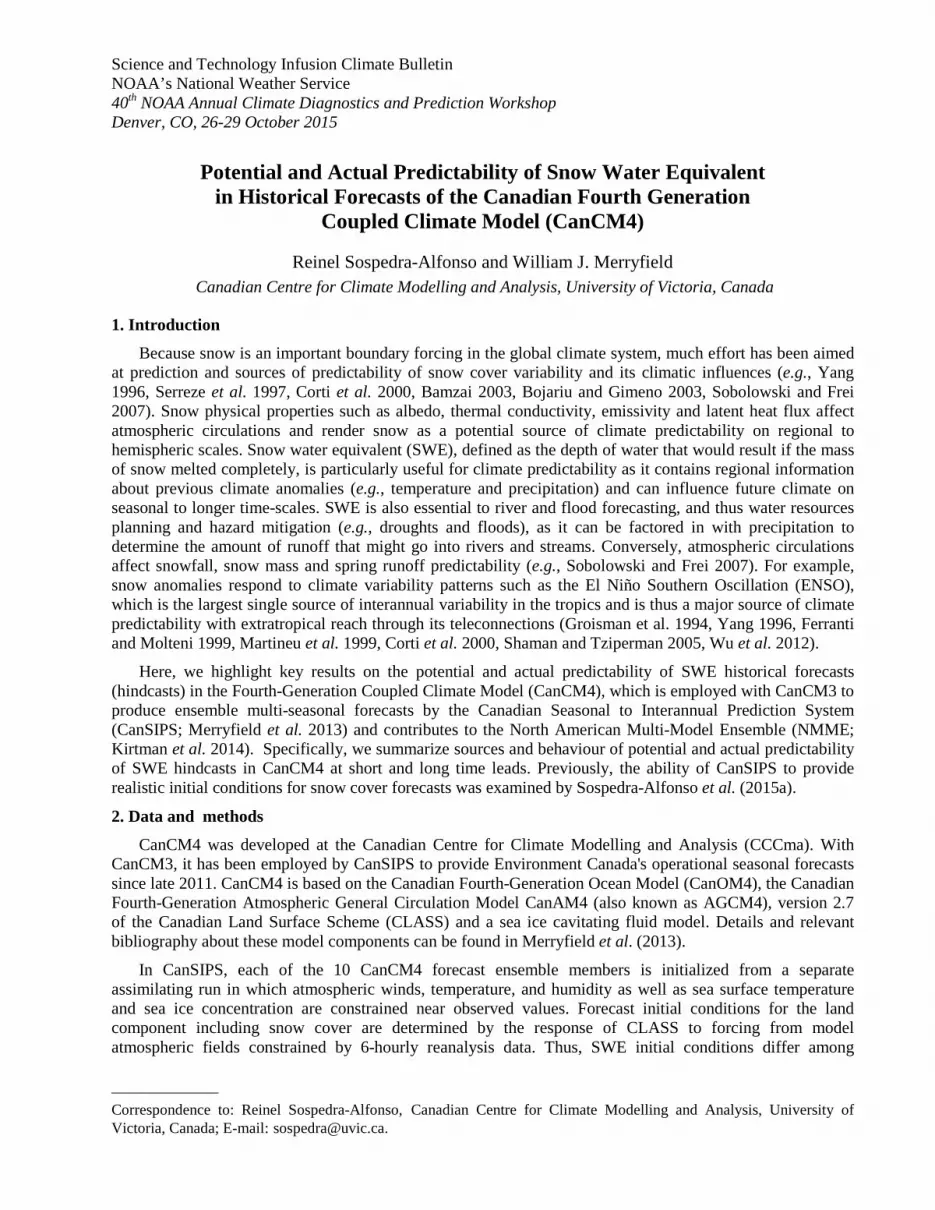
Science and Technology Infusion Climate Bulletin NOAA’s National Weather Service 40th NOAA Annual Climate Diagnostics and Prediction Workshop Denver, CO, 26-29 October 2015
______________
Correspondence to: Reinel Sospedra-Alfonso, Canadian Centre for Climate Modelling and Analysis, University of Victoria, Canada; E-mail: [email protected].
Potential and Actual Predictability of Snow Water Equivalent in Historical Forecasts of the Canadian Fourth Generation
Coupled Climate Model (CanCM4)
Reinel Sospedra-Alfonso and William J. Merryfield Canadian Centre for Climate Modelling and Analysis, University of Victoria, Canada
1. Introduction
Because snow is an important boundary forcing in the global climate system, much effort has been aimed at prediction and sources of predictability of snow cover variability and its climatic influences (e.g., Yang 1996, Serreze et al. 1997, Corti et al. 2000, Bamzai 2003, Bojariu and Gimeno 2003, Sobolowski and Frei 2007). Snow physical properties such as albedo, thermal conductivity, emissivity and latent heat flux affect atmospheric circulations and render snow as a potential source of climate predictability on regional to hemispheric scales. Snow water equivalent (SWE), defined as the depth of water that would result if the mass of snow melted completely, is particularly useful for climate predictability as it contains regional information about previous climate anomalies (e.g., temperature and precipitation) and can influence future climate on seasonal to longer time-scales. SWE is also essential to river and flood forecasting, and thus water resources planning and hazard mitigation (e.g., droughts and floods), as it can be factored in with precipitation to determine the amount of runoff that might go into rivers and streams. Conversely, atmospheric circulations affect snowfall, snow mass and spring runoff predictability (e.g., Sobolowski and Frei 2007). For example, snow anomalies respond to climate variability patterns such as the El Niño Southern Oscillation (ENSO), which is the largest single source of interannual variability in the tropics and is thus a major source of climate predictability with extratropical reach through its teleconnections (Groisman et al. 1994, Yang 1996, Ferranti and Molteni 1999, Martineu et al. 1999, Corti et al. 2000, Shaman and Tziperman 2005, Wu et al. 2012).
Here, we highlight key results on the potential and actual predictability of SWE historical forecasts (hindcasts) in the Fourth-Generation Coupled Climate Model (CanCM4), which is employed with CanCM3 to produce ensemble multi-seasonal forecasts by the Canadian Seasonal to Interannual Prediction System (CanSIPS; Merryfield et al. 2013) and contributes to the North American Multi-Model Ensemble (NMME; Kirtman et al. 2014). Specifically, we summarize sources and behaviour of potential and actual predictability of SWE hindcasts in CanCM4 at short and long time leads. Previously, the ability of CanSIPS to provide realistic initial conditions for snow cover forecasts was examined by Sospedra-Alfonso et al. (2015a).
2. Data and methods
CanCM4 was developed at the Canadian Centre for Climate Modelling and Analysis (CCCma). With CanCM3, it has been employed by CanSIPS to provide Environment Canada's operational seasonal forecasts since late 2011. CanCM4 is based on the Canadian Fourth-Generation Ocean Model (CanOM4), the Canadian Fourth-Generation Atmospheric General Circulation Model CanAM4 (also known as AGCM4), version 2.7 of the Canadian Land Surface Scheme (CLASS) and a sea ice cavitating fluid model. Details and relevant bibliography about these model components can be found in Merryfield et al. (2013).
In CanSIPS, each of the 10 CanCM4 forecast ensemble members is initialized from a separate assimilating run in which atmospheric winds, temperature, and humidity as well as sea surface temperature and sea ice concentration are constrained near observed values. Forecast initial conditions for the land component including snow cover are determined by the response of CLASS to forcing from model atmospheric fields constrained by 6-hourly reanalysis data. Thus, SWE initial conditions differ among

SCIENCE AND TECHNOLOGY INFUSION CLIMATE BULLETIN
130
ensemble members. CanSIPS hindcasts are initialized at the beginning of each month during a multidecadal hindcast period and have a 12 month range.
We consider CanCM4 SWE hindcasts (1981–2010) in the Northern Hemisphere on the approximately 2.8° atmospheric/land surface model grid. We employ the following metrics:
• Potential predictability (PP) of monthly mean SWE in CanCM4 is examined by employing analysis of variance (ANOVA) (e.g., von Storch and Swiers 1999) on the 10 ensemble members to estimate the fraction of internnual SWE variability that is potentially predictable. In this framework, the total interannual variability of SWE is partitioned into two components; (1) unpredictable chaotic fluctuations or noise, and (2) potentially predictable variability or “signal” variance associated with internal climate variability modes (e.g., ENSO) and/or external forcing (e.g., solar variability, explosive volcano eruptions, anthropogenic radiative forcing). The potential predictability of SWE is defined as the ratio of the signal to the total variance.
• Persistence of initial anomalies in CanCM4 SWE forecasts is given in terms of the temporal autocorrelation (AC) of predicted SWE anomalies, which is defined as the correlation between SWE forecast anomalies and the initial ensemble mean anomaly, averaged across the ensemble. The initial ensemble mean anomaly is employed instead of initial anomalies of individual ensemble members to account for uncertainty in the initial conditions of SWE anomalies, which results in a degradation of autocorrelation at the zero lead time. AC2 is a measure of the fraction of SWE variability that can be linearly attributed to the initial SWE anomalies, and can be compared with PP of SWE to assess the contribution of the memory of snowpack initial conditions to the potential predictability.
• ENSO influence on SWE is investigated by regressing CanCM4 forecast monthly mean SWE, surface temperature and precipitation on the monthly Niño 3.4 index (defined as the averaged sea surface temperature anomaly over the Pacific Ocean region 5°S-5°N, 120°-170°W).
• Actual skill in CanCM4 SWE forecasts is examined by computing the temporal anomaly correlation coefficient (ACC) between forecasts ensemble mean and a blend of 5 SWE observation-based products (Blended-5) developed by Mudryk et al. (2015), re-gridded to CanSIPS resolution. Blended-5 combines SWE from (1) the National Aeronautics and Space Administration (NASA) Modern-Era Retrospective analysis for Research and Application (MERRA; Rienecker et al. 2011), (2) the European Centre for Medium-Range Forecasts Interim Land Reanalysis (ERA-Interim/Land; Balsamo et al. 2013), (3) GlobSnow analysis, version 2, developed through the European Space Agency GlobSnow project and produced by the Finnish Meteorological Institute (Takala et al. 2011), (4) the Global Land Data Assimilation System Version 2 (GLDAS-2) product (Rodell et al. 2004), and (5) the Crocus snow scheme driven by ERA-Interim (Brun et al. 2013).
3. Summary of results and discussion
We identify two main sources of potential predictability and actual skill in CanCM4 SWE forecasts: (i) persistence of initial SWE anomalies, and (ii) SWE response to climate variations that are potentially predictable at longer time-scales, including ENSO.
Fig. 1 Scatter plots of Northern Hemisphere spatial means of AC2 for CanCM4 (vertical axis) vs (a) PP for CanCM4 (horizontal axis) and (b) AC2 for Blended-5 (horizontal axis) for each month and lead time in the forecast. Dots correspond to target months and colors denote lead times.

SOSPEDRA-ALFONSO AND MERRYFIELD
131
SWE depends cumulatively on previous snowfall and snowmelt events, therefore this “memory” in the form of anomaly persistence should contribute to PP. Spatial averages of PP and AC2 over the Northern Hemisphere tend to be large and comparable to each other for short lead times (0-2 months) and much smaller for longer leads (over 4-month), with values that depend on the target month and initialization date (Fig. 1a). The short-range behaviour of PP is thus strongly determined by the persistence of initial SWE anomalies, particularly in regions of mature snowpack and/or initialization times in the core of the snow season. For example, for March-averaged SWE forecasts at 1-month lead (i.e., initialized in February), which is prior to the start of the snowmelt and long after the snow onset in the mid-latitudes, high PP (> 0.8) occurs in the higher latitudes (> 60°N), western Canada, and the Karakoram region (Fig. 2a). Geographic patterns of AC2 (not shown) indicate that these regions are characterized by high SWE anomaly persistence.
PP determined by SWE anomaly persistence tends to decrease with lead time as the result of a relative increase in noise variance (due to ensemble dispersion), and with decreasing latitude and/or elevation due to a relative decrease in signal variance associated with shorter snow seasons. For example, PP of March-averaged SWE at 11-month lead is insignificant (< 0.1) in most of the Northern Hemisphere, with the exception of the Pacific Northwest, the southern Rocky Mountains and Karakoram (up to ≈ 0.5), and a few scattered regions in Asia and North America (Fig. 2b).
Spatially averaged AC2 in CanCM4 SWE forecasts behaves similarly to that of the verifying observations (Fig. 1b). This suggests that CanCM4 should capitalize on SWE anomaly persistence as a source of actual skill, at least for short lead times. For example, ACC2 for March-averaged SWE forecasts at 1-month lead (Fig. 2c) has similar geographic patterns as PP (Fig. 2a), except in the Tibetan Plateau where PP is relatively high but ACC2 is <0.1. As for PP, ACC2 tends to decay with lead time and is statistically insignificant at 11-month lead in most of the Northern Hemisphere, with the exception of the Pacific Northwest, the Karakoram region and a few scattered regions in Asia and North America (Fig. 2d).
The long-range behaviour of PP in CanCM4 (e.g., Fig. 2b) is likely the result of SWE response to ENSO variability, combined with the ability of the forecasts to predict ENSO. Regression patterns of December and March-averaged SWE in forecasts initialized in the preceding April show that the regions where March-averaged SWE is potentially predictable (Fig. 2b) largely correspond with those where SWE anomalies associated with ENSO variability are statistically significant (Figs. 3a, b).
Fig. 2 (top) PP and (bottom) ACC2 against Blended-5 of CanCM4 March-averaged SWE forecasts at (left) 1-month and (right) 11-month lead times indicating the time from forecast initial values.

SCIENCE AND TECHNOLOGY INFUSION CLIMATE BULLETIN
132
SWE response to ENSO is likely driven by ENSO influences on temperature (T) and precipitation (P). Because of the SWE anomaly persistence discussed earlier, T and P influence on SWE is not limited to contemporary months but has contributions from previous months in the snow season (e.g., Sospedra-Alfonso et al. 2015b). For example, regression patterns of December and March-averaged T and P corresponding to the forecasts initialized in April (Figs. 3c-f) reveal that negative anomalies of March-averaged SWE (Fig. 3b) in western Canada are likely the result of positive T and negative P anomalies already present in December (Fig. 3c, e) and November (not shown). This is likely the reason for the increased amplitude of ENSO-related SWE anomalies in March relative to December (Fig. 3a, b). Positive anomalies of December-averaged SWE (Fig. 3a) found in the southern U.S. Rocky Mountains are most likely due to negative T and positive P anomalies in December (Fig. 3c, e) and November (not shown). In the Karakoram, statistically significant positive anomalies of December-averaged SWE (Fig. 3a) are associated with positive P anomalies in December (Fig. 3e) and November (not shown), despite the slightly positive T anomalies in the region. These results support the idea that relatively high values of PP (Fig. 2b) and actual skill (Fig. 2d) for March-averaged SWE in the western North America and the Karakoram at 11-month lead is a signature of ENSO teleconnections.
4. Concluding remarks
CanCM4 forecasts of SWE can display appreciable potential and actual skill depending on region, target month and initialization date. The behaviour of PP of SWE at short leads can be largely explained in terms of persistence of initial anomalies. Exploiting this source of PP as actual skill thus requires a reasonably accurate initialization of SWE, as occurs in CanSIPS (Sospedra-Alfonso et al. 2015a). The relative contribution of anomaly persistence to PP diminishes at longer lead times, implying that ability to predict future climate anomalies (e.g., temperature and precipitation anomalies) contributes increasingly to PP as lead time increases. For long leads, PP of CanCM4 SWE forecasts appears to be mainly the result of SWE response to ENSO variability, combined with the ability of the forecasts to predict ENSO.
Fig. 3 Regressions of CanCM4 predicted (left) December and (right) March averaged (a, b) SWE, (c, d) surface air temperature and (e, f) precipitation against CanCM4 predicted Niño 3.4 index for the forecasts initialized in April. Lead times are (left) 8 months and (right) 11 months. Cross hatched regions correspond to correlations >0.3.

SOSPEDRA-ALFONSO AND MERRYFIELD
133
Disclaimer. This note complements a detailed work on potential and actual predictability of snow in CanSIPS submitted for publication in the Journal of Hydrometeorology.
References
Balsamo, G., and Coauthors, 2013: ERA-Interim/Land: a global land water resources dataset. Hydrology and Earth System Sciences Discussions, 10, 14,705–14,745.
Bamzai, A. S., 2003: Relationship of snow cover variability and Arctic oscillation index on a hierarchy of time scales. International Journal of Climatology, 23, 131–142.
Bojariu, R., and L. Gimeno, 2003: The role of snow cover fluctuations in multiannual NAO persistence. Geophysical Research Letters, 30, 1156.
Brun, E., V. Vionnet, A. Boone, B. Decharme, Y. Peings, R. Valette, F. Karbou, and S. Morin, 2013: Simulation of northern Eurasian local snow depth, mass, and density using a detailed snowpack model and meteorological reanalyses. Journal of Hydrometeorology, 14, 203–219.
Corti, S., F. Molteni, and Č. Branković, 2000: Predictability of snow-depth anomalies over Eurasia and associated circulation patterns. Quarterly Journal of Royal Meteorological Society, 126, 241–262.
Ferranti, L., and F. Molteni, 1999: Ensemble simulations of eurasian snow-depth anomalies and their influence on the summer asian monsoon. Quarterly Journal of the Royal Meteorological Society, 125, 2597–2610.
Groisman, P. Y., T. R. Karl, and R. W. Knight, 1994: Changes of snow cover, temperature, and radiative heat balance over the northern hemisphere. Journal of Climate, 7, 1633–1656.
Kirtman, B., and Coauthors, 2014: The North American Multimodel Ensemble: Phase-1 seasonal-to-interannual prediction; Phase-2 toward developing intraseasonal prediction. Bulletin of the American Meteorological Society, 95, 585–601.
Martineu, C., J.-Y. Caneill, and R. Sadourny, 1999: Potential predictability of European winters from the analysis of seasonal simulations with an AGCM. Journal of Climate, 12, 3033–3061.
Merryfield, W. J., W.-S. Lee, G. J. Boer, V. V. Kharin, J. F. Scinocca, G. M. Flato, R. S. Ajayamohan, and J. C. Fyfe, 2013: The Canadian Seasonal to Interannual Prediction System. Part I: Models and Initialization. Monthly Weather Review, 141, 2910–2945.
Mudryk, L. R., C. Derksen, P. J. Kushner, and R. Brown, 2015: Characterization of Northern Hemisphere snow water equivalent datasets, 1981-2010. Journal of Climate, 28, 8037–8051.
Rienecker, M. M., and Coauthors, 2011: MERRA - NASA’s modern-era retrospective analysis for research and applications. Journal of Climate, 24, 3624–3648.
Rodell, M., and Coauthors, 2004: The Global Land Data Assimilation System. Bulletin of the American Meteorological Society, 85, 381–394.
Serreze, M. C., F. Carse, R. G. Barry, and J. C. Rogers, 1997: Icelandic low cyclone activity: Climatological features, linkages with the NAO, and relationships with recent changes in the Northern Hemispheric circulation. Journal of Climate, 10, 453–464.
Shaman, J., and E. Tziperman, 2005: The effect of ENSO on Tibetan Plateau snow depth: A stationary wave teleconnection mechanism and implications for the south Asian Monsoons. Journal of Climate, 18, 2067–2079.
Sobolowski, S., and A. Frei, 2007: Lagged relationships between North American snow mass and atmospheric teleconnections indices. International Journal of Climatology, 27, 221–231.
Sospedra-Alfonso, R., L. Mudryk, W. J. Merryfield, and C. Derksen, 2015a: Representation of snow in the Canadian Seasonal to Interannual Prediction System: Part I. Initialization. Journal of Hydrometeorology. doi: 10.1175/JHM-D14-0223.1
Sospedra-Alfonso, R., J. R. Melton, and W. J. Merryfield, 2015b: Effects of temperature and precipitation on snowpack variability in the Central Rocky Mountains as a function of elevation. Geophysical Research Letters, 42, 4429–4438.

SCIENCE AND TECHNOLOGY INFUSION CLIMATE BULLETIN
134
Takala, M., K. Luojus, J. Pulliainen, C. Derksen, J. Lemmetyinen, J.-P. Karna, J. Koskinen, and B. Bojkov, 2011: Estimating northern hemisphere snow water equivalent for climate research through assimilation of space-borne radiometer data and ground-based measurements. Remote Sensing of Environment, 115, 3517–3529.
von Storch, H., and F. W. Zwiers, 1999: Statistical Analysis in Climate Research. Cambridge University Press, 484 pp.
Wu, Z., J. Li, Z. Jiang, and T. Ma, 2012: Modulation of the Tibetan Plateau snow cover on the ENSO teleconnections: From the east Asian summer monsoon perspective. Journal of Climate, 25, 2481–2489.
Yang, S., 1996: ENSO-snow-monsoon associations and seasonal-interannual predictions. International Journal of Climatology, 16, 125–134.

Science and Technology Infusion Climate Bulletin
NOAA’s National Weather Service
40th NOAA Annual Climate Diagnostics and Prediction Workshop
Denver, CO, 26-29 October 2015
______________
Correspondence to: Bhaskar Jha, 5830 University Research Court, Climate Prediction Center, NOAA/NWS/NCEP,
College Park, Maryland; E-mail: [email protected].
An Analysis of Predictability of Seasonal Atmospheric Variability
Using NMME Models
Bhaskar Jha1,2
and Arun Kumar1
1Climate Prediction Center, NOAA/NWS/NCEP, College Park, Maryland 2 Innovim LLC, Greenbelt, Maryland
The seasonal predictability of 200-hPa height (Z200) was estimated based on North American Multi-
Model Ensemble (NMME) forecast system. In this analysis, a simple procedure was adopted based on finding
the minimum value of Mean Square Error (MSE) between observed and NMME forecast system (Kumar et al.
2007) and it was argued that the minimum MSE is a best estimate of the atmospheric seasonal internal
variability.
The updated estimates of seasonal
internal variability based on NMME
forecast show significant reduction in
MSE over tropical region as compared to
Atmospheric Modeling Intercomparison
Project (AMIP) and Development of
European Multimodel Ensemble System
for Seasonal to Interannual Prediction
(DEMETER) based estimates. The top
and middle panels of Fig. 1 are based on
AMIP simulation and DEMETER data
sets (Kumar et al. 2007) and bottom
panel is the current estimate of seasonal
internal variability based on NMME
forecast. However, the amplitude of
seasonal internal variability based on
NMME forecast system shows little
reduction over Pacific North America
(PNA), Greenland region, northern and
southern higher latitude compared to
AMIP and DEMETER. Overall seasonal
observed variability looks broadly similar
over northern and southern higher latitude.
In this work, the analysis was focused
on predictability of Z200 in Northern Hemisphere winter. It is clear that the predictability should be seasonal
and variable dependent, e.g. it is expected that the predictability is lower in Northern Hemisphere summer
than in winter, which needs further investigation.
Last, next generation forecast system and corresponding spatial map of MSE can be used to update the
spatial map of internal variability as well as the predictability. It remains to be seen how much of the internal
variability estimates based on NMME forecast (Fig. 1 bottom panel), can be further improved because of
improved models by higher resolution, better initial condition and larger ensemble sizes. The present estimate
can be used as a benchmark that could be used to document such improvement.
This work has been submitted to Climate Dynamics.
Fig. 1 The internal variance from grid-to-grid point is best
estimated by the minimum value of MSE. Left panel (top)
for AMIP, (middle) for DEMETER and (bottom) for
NMME. The right panel is the same plot as the left panel
except for shading that indicates the significance of
estimated MSE at 95% level based on Monte Carlo
approach.

SCIENCE AND TECHNOLOGY INFUSION CLIMATE BULLETIN
136
Acknowledgements. This study was supported by NOAA's Climate Program Office's Modeling, Analysis,
Predictions, and Projections program.
References
Kumar, A., B. Jha, Q. Zhang, and L. Bounoua, 2007: A new methodology for estimating the unpredictable
component of seasonal atmospheric variability. J. Climate, 20, 3888-3901.

Science and Technology Infusion Climate Bulletin NOAA’s National Weather Service 40th NOAA Annual Climate Diagnostics and Prediction Workshop Denver, CO, 26-29 October 2015
______________
Correspondence to: Kirstin J. Harnos, 5830 University Research Court, Climate Prediction Center, NOAA/NWS/NCEP, College Park, Maryland; E-mail: [email protected]
Comparison of Warm Season North American Precipitation Variability Observations to CFSv2
Kirstin J. Harnos1, 2 and Scott J. Weaver1, 3 1Climate Prediction Center, NOAA/NWS/NCEP, College Park, Maryland
2Innovim LLC, Greenbelt, Maryland 3Enviornmental Defense Fund
1. Introduction
Warm season precipitation, defined as April/May/June (AMJ), in the central and eastern US is driven by the northward transport of heat and moisture by the low-level atmospheric circulation (the North American low-level Jet; NALLJ). The NALLJ’s main role in the climate system is to communicate the large scale climate influences (i.e. sea surface temperature; SST) to regional scales. Thus understanding SST influences on NALLJ variability is fundamental to understanding how the large scale remote climate influences are manifest in the context of regional climate variability and change.
Previous studies have shown significant correlations between NALLJ variability and modes of SST are present from 1950-2010. However, the extent of influence SSTs have on NALLJ and regional precipitation variability is difficult to obtain from observations alone. To further characterize SST influence on NALLJ and precipitation variability, the observational analyses are repeated using the National Center for Environmental Prediction Climate Forecast System Version 2 (CFSv2) Atmospheric Model Intercomparison Project (AMIP) simulations.
2. Data
This study utilizes multiple datasets due to its focus on comparing observations to simulations. Rainfall observations are from the Precipitation Reconstruction updated by the NOAA Climate Prediction Center (CPC) and are available from the CPC website. The NALLJ observations are identified from the 850hpa V-wind from the NCAR/NCEP reanalysis. With the main goal of determining SST influence on precipitation variability, the ERSSTv3 SST dataset is chosen to determine the correlation between SSTs and the NALLJ observations. The simulated dataset is from the CFSv2 AMIP dataset. The simulations consist of 12 ensemble members with monthly output from 1950-2010. Isolating the SST influence from the CFSv2 AMIP simulations is accomplished by comparing the ensemble mean value to the observations.
Fig. 1 Correlations between the first 3 modes of the NALLJ and the SST observations.

SCIENCE AND TECHNOLOGY INFUSION CLIMATE BULLETIN
138
3. Summary of results
(a) NALLJ and SST
The first three modes of the EOF analysis performed on the NALLJ region bounded by 105° – 80°W 20° – 50°N are correlated to the SST observations for 1950-2010 (Figure 1). Mode 1 accounts for approximately 41% of the variance. It also shows the strongest correlations with the largest values in the North Pacific. Correlation patterns in the Pacific are similar to spatial pattern of the Pacific Decadal Oscillation. Atlantic correlations are weaker than the Pacific with a spatial pattern similar to the Atlantic Multidecadal Oscillation. Mode 2 accounts for approximately 20% of the variance with the weakest correlations of the three modes. Mode 3 accounts for approximately 11 % of the variance with correlations focused in the tropical pacific region.
(b) Precipitation & 850hpa V-wind climatology
The observations of the AMJ NALLJ stretches from the western Gulf of Mexico into the central plains with the NALLJ maximum centered over Texas. Precipitation observations are focused east of NALLJ position in the Southern Plains and Southeastern regions. CFSv2 AMIP NALLJ is centered over same region as observations. AMIP NALLJ is stronger than observations with tighter gradient along topography in western Texas. AMIP precipitation is focused further north in Great Plains region.
(c) Precipitation variability (standard deviation)
Comparisons of the precipitation are shown in Figure 2. The largest variability is focused in Southern Great Plains and Southeastern regions. Observations and total AMIP mean in relative agreement in location and magnitude of variability with total AMIP slightly larger (around .2 mm day-1) in Northern Plains region. The SST influence is greatest over Southern Plains and Southeastern US with values slightly less than half of both the observed and AMIP total.
(d) Regional breakdown
Figure 3 gives the regional breakdown of the precipitation variability. For the Northern Great Plains, the observations fall within envelope of AMIP ensemble spread. The moving standard deviation AMIP mean value (isolating SST influence) is around 0.1 which accounts for around 25% of total variability. For the Southern Great Plains, the observations fall within the AMIP spread. AMIP mean value varies from 0.2 to 0.4 which accounts for around 30% of the total variability. Finally, the Southeast region, the observations fall
Fig. 2 Comparison of precipitation variability from the observations (top panel) to the total AMIP mean (middle panel) and the AMIP mean isolating SST influence (bottom panel).
Fig. 3 30-year moving standard deviation of precipitation (mm/day) for the Northern Great Plains (left panel), Southern Great Plains (middle panel), and the Southeast (right panel). Dashed black line is the total AMIP mean with light blue shading indicating the ensemble spread. Red line is the observations. Dark blue line is the AMIP mean isolating the SST influence.

HARNOS AND WEAVER
139
within the spread of the ensemble. The AMIP mean value is around 0.4 which accounts for about 50% of the total variability.
4. Discussion
There are similar spatial patterns between observations and CFSv2 for NALLJ location, with a slightly stronger jet and larger precipitation values in CFSv2 AMIP dataset. Precipitation variability as represented by precipitation standard deviation shows similar spatial patterns when comparing observations and total AMIP variability. AMIP SST influence shows largest variability over Southern Plains and Southeastern US with values slightly less than half of both the observed and AMIP total. Regional comparisons of precipitation anomalies show observations fall within spread of all 12 AMIP ensemble members. Moving standard deviations of regional variability show SST AMIP mean below observations and ensemble spread. SST influence accounts for anywhere from ~25 – 50% of the total variability.
Acknowledgements. This study was supported by NOAA's Climate Program Office's Modeling, Analysis, Predictions, and Projections program.

Science and Technology Infusion Climate Bulletin NOAA’s National Weather Service 40th NOAA Annual Climate Diagnostics and Prediction Workshop Denver, CO, 26-29 October 2015
______________
Correspondence to: Yana Li, School of Atmospheric Sciences, Sun Yat-sen University, Guangzhou, China; E-mail: [email protected].
Feedback Attributions of the Climate Difference in the Muted and the Accelerated Warming Periods
Yana Li1, Xiaoming Hu1, Song Yang1, Ming Cai2, Yi Deng3 1School of Atmospheric Sciences, and Institute of Earth Climate and Environment System
Sun Yat-sen University, Guangzhou, China 2Department of Earth, Ocean, and Atmosphere Science, Florida State University, Tallahassee, FL, USA
3School of Earth and Atmospheric Sciences, Georgia Institute of Technology, Atlanta, GA, USA
1. Data and methodology
Most of the data used in this study are obtained from the latest European Centre for Medium-range Weather Forecasts (ECMWF) Re-Analysis Interim (ERA-Interim; Uppala et al. 2008; Dee et al. 2011). The time series of the annual mean CO2 concentration from 1984 to 2013 is downloaded from the Earth System Research Laboratory website (http://www.esrl.noaa.gov/gmd/ccgg/trends/).
We have adopted the same package of a climate feedback-response analysis method (CFRAM) analysis reported in Deng et al. (2012) and Sejas et al. (2014) to attribute the near-surface temperature anomalies (STAs) shown in Fig. 1c to external forcing and various climate feedback processes (radiative and non-radiative feedback processes, shown in Equation (1)), based on the energy balance.
∆T𝑀+1 = �∂R��⃗
∂T��⃗�𝑀+1
−1�
∆S�⃗ (solar) + ∆R��⃗ (𝐶𝐶2) + ∆S�⃗ (α) + �∆S�⃗ (w) − ∆R��⃗ (w)�+ �∆S�⃗ (c) − ∆R��⃗ (c)�+�∆S�⃗ �O3� − ∆R��⃗ �O3��+ ∆Q��⃗ 𝐿𝐿 + ∆Q��⃗ 𝑆𝐿 + ∆Q��⃗ 𝑜𝑜𝑜_𝑑𝑑𝑜+𝑠𝑠𝑜𝑠𝑠𝑠𝑠 + ∆Q��⃗ 𝑠𝑠𝑎_𝑑𝑑𝑜
� (1)
2. Results
The decade of 1984-95 is regarded as the accelerated warming period whereas the decade of 2002-13 corresponds to a weaker warming period. This work examines the mean state difference between the two periods (Fig. 1). The key features of the mean state in 2002-13 in reference to that in the accelerated warming period are (i) a La Niña like pattern over the tropical Pacific, (ii) a pronounced polar warming amplification pattern in the northern extratropics, and (iii) cold temperature anomalies over the Southern Ocean sandwiched by the dominance of warm temperature anomalies in the north and
Fig. 1 Annual mean STAs of the period of (a) 1984-95, and (b) 2002-13, (Unit: K). (c) The difference in SAT between the two periods (Unit: K). And (d) the sum of CFRAM-derived partial temperature changes due to individual processes. The dotted areas indicate values achieving 0.1 level of statistical significance. The blue box outlines the tropical Pacific region (20°S-20°N, 150°-100°W), one of the three key regions discussed in the text.

LI ET AL.
141
south in the southern extratropics.
A climate feedback-response analysis method is applied to attribute the changes in the climatological mean surface temperature between the two periods to various dynamic and thermodynamic processes (Fig. 2). The La Niña like pattern is associated with the strengthening of the Walker Circulation over the tropical Pacific. Increase of low level clouds, reduction of atmospheric water vapor, and increase of surface latent heat fluxes are the main processes contributing to the cooling in the eastern tropical Pacific. Surface processes contribute positively to the spatial pattern of the mean state difference in both the northern and southern extratropics. The atmospheric dynamic processes contribute positively to the difference in the northern extratropics, but negatively to the difference in the southern extratropics, responsible for the greater warming over the northern extratropics than the southern extratropics (Fig. 3; Note that the term labeled as “Others” is for the sum of partial STAs due to differences in solar radiation, CO2, and ozone between the two periods whereas the “Sum” is the PAP coefficient obtained from the sum of all CFRAM-derived STAs. Bars with dots overlay the corresponding bars labeled with “Sum”, indicating that the sum of all CFRAM-derived STAs indeed approximates to observed STAs.).
References
Dee, D. P., S. M. Uppala, A. J. Simmons, P. Berrisford, P. Poli, S. Kobayashi, U. Andrae, M. A. Balmaseda, G. Balsamo et al, 2011: The ERA-Interim reanalysis: configuration and performance of the data assimilation system. Q. J. R. Meteorol. Soc., 137, 553-597.
Deng, Y., T. Park and M. Cai, 2012: Process-based decomposition of the global surface temperature response to El Niño in boreal winter. J. Atmos. Sci., 69, 1706-1712.
Fig. 2 Partial STAs (units: K) due to the (a) surface processes (including surface sensible heat flux, surface latent heat flux, and the oceanic dynamic process plus ocean/land heat storage term), (b) atmospheric dynamic processes, (c) water vapor feedback, and (d) cloud feedback.
Fig. 3 Pattern-amplitude projection (PAP) coefficients (units: K) of the CFRAM-derived partial STAs associated with various radiative and non-radiative processes in (a) Tropical Pacific, (b) Northern extratropics (30°-90°N)and (c) Southern extratropics (30°-90°S).

SCIENCE AND TECHNOLOGY INFUSION CLIMATE BULLETIN
142
Sejas, S. A., M. Cai, A.-X. Hu, G. A. Meehl, W. Washington, and P. C. Taylor, 2014: Individual feedback contributions to the seasonality of surface warming. J. Climate, 27, 5653–5669.
Uppala, S. M., D. Dee, S. Kobayashi, P. Berrisford, A. Simmons, 2008: Towards a climate 500 data-assimilation system: Status update of ERA–Interim. ECMWF Newsletter, 115, 12-18.

Science and Technology Infusion Climate Bulletin NOAA’s National Weather Service 40th NOAA Annual Climate Diagnostics and Prediction Workshop Denver, CO, 26-29 October 2015
______________
Correspondence to: Wei Wei, School of Atmospheric Sciences, Sun Yat-sen University, Guangzhou, China; E-mail: [email protected].
Relationship between the Asian Westerly Jet Stream and Summer Rainfall over Central Asia and North China:
Roles of the Indian Monsoon and the South Asian High
Wei Wei1, 2, Renhe Zhang2, Min Wen2, and Song Yang1 1School of Atmospheric Sciences, Sun Yat-sen University, Guangzhou, China
2State Key Laboratory of Severe Weather, Chinese Academy of Meteorological Sciences, Beijing, China
1. Introduction
Over the Eurasian continent, the summertime upper-tropospheric westerlies are located around 40ºN where the Asian westerly jet stream (AWJS) exists. Diagnostic analyses are performed to investigate the relationship between the AWJS and the associated rainfall pattern over the AWJS region in boreal summer on interannual time scales. The physical mechanisms on the relationship between the AWJS and the rainfall pattern are revealed by exploring the effects of the Indian summer monsoon (ISM) and the South Asian high (SAH).
The interannual variation of the AWJS is depicted by the principal component of the first EOF mode of the 200-hPa zonal wind over the AWJS region (u200_PC1). It indicates the significant southeast-northwest (SE-NW) fluctuation of the AWJS. The South Asian high index (SAHI: Z200(20º-27.5ºN,
85º-115ºE) minus Z200(27.5º-35ºN, 50º-80ºE)) defined by Wei et al. (2015) provides an accurate depiction of the SE-NW displacement of the SAH. And we also use the all-India rainfall index (AIRI) to measure the intensity of the ISM. These indices are employed to analyze the relationships of the SAH, AWJS and ISM with the rainfall over the AWJS region.
2. Summer rainfall over the AWJS region
A regression analysis of summer rainfall against the SAHI shows a pronounced inverse relationship between the arid region in central Asia (CA) and the monsoon region in North China (NC) (Fig. 1). Such a relationship indicates that when the SAH moves to the southeast, rainfall increases to the northwest of the Tibetan Plateau (TP) over CA and decreases in the monsoon region of the same latitudes over NC (Fig. 1a). Figure 1b provides a zonal distribution of regressed rainfall anomalies along 36º-41ºN. It illustrates that positive anomalies
Fig. 1 (a) Regressed JJA rainfall anomalies against the SAHI (shadings; unit: mm). Areas exceeding the 0.05 significance level are highlighted by thick contours. Mid-latitude CA (36º-41ºN, 70º-90ºE) and NC (36º-41ºN, 105º-120ºE) regions are indicated by red boxes. (b) Zonal distribution of regressed JJA rainfall anomalies along 36º-41ºN. (c) Standardized time series of CA rainfall (blue solid line) and NC rainfall (red dashed line) from 1958 to 2002.

SCIENCE AND TECHNOLOGY INFUSION CLIMATE BULLETIN
144
consistently appear to the west of about 102ºE, with the maximum value at approximately 70º-80ºE. To the east of about 102ºE, negative rainfall anomalies enhance from the west to the east. Affected by the EASM, the rainfall anomalies over NC is much larger than those over CA. Figure 1c shows the time series for standardized summer rainfall over CA (36º-41ºN, 70º-90ºE) and NC (36º-41ºN, 105º-120ºE). The out-of-phase relationship of the summer rainfall over these two regions is obvious on interannual time scale. The coefficient of correlation between the rainfalls over CA and NC is -0.33, which exceeds the 0.05 significance level.
The out-of-phase variations in the rainfall over the AWJS region are significantly related to the fluctuations of the AWJS, the SAH, and the ISM (see Table 1). When the ISM is weak, the AWJS and the SAH shift to the southeast, and the summer rainfall increases in the arid CA region and decreases in NC of the EASM region. Moreover, the significant correlation (see Table 1) among these three systems indicates that the fluctuations of these three systems may be interdependent from each other.
Table 1 Correlation coefficients among rainfall over CA, NC, SAHI, u200_PC1, and AIRI
Note: * and * * indicate correlation coefficients exceeding the 0.01 and 0.05 significance level, respectively.
3. Physical links among the SAH, AWJS and ISM
3.1 Effect of SAH on the AWJS rainfall
A regression analysis of the circulation anomalies at 200 hPa against the SAHI shows that when the SAH moves to the southeast, the anomalous cyclone to the northwest of TP strengthens the westerlies to the south of the AWJS and causes a southward movement of the AWJS (Fig. 2). In the eastern portion of the AWJS over the EASM region, strong anomalous northwesterlies are generated between the anomalous cyclone over northeastern Asia and the anomalous anticyclone to the southeast of the TP, and move the AWJS to the southeast. Therefore, the anomalous circulation associated with the SE-NW fluctuation of the SAH is responsible for the SE-NW variation of the AWJS. When the SAH moves to the southeast, the southeastward located AWJ will intensify the upper-level divergence over CA and the upper-level convergence over NC. As a result, there are more rainfall in CA and less rainfall in NC.
CA_Rainfall NC_Rainfall SAHI u200_PC1 AIRI
CA_Rainfall 1.00
NC_Rainfall -0.33** 1.00
SAHI 0.63* -0.53* 1.00
u200_PC1 0.68* -0.47* 0.73* 1.00
AIRI -0.37** 0.47* -0.64* -0.52* 1.00
Fig. 2 Regressed circulation (vectors; unit: m s-1) and divergence (shadings; unit: 10-6 s-1) anomalies against the SAHI at 200 hPa. Westerly jet stream (blue contours) and SAH (red contours) are represented by the composited values of 30 m s-1 and 12520 gpm (contours), respectively, for SAHI larger than 1 (solid line) and smaller than -1 (dashed line). Contours in green indicate the TP region with elevations exceeding 3000 m.

WEI ET AL.
145
3.2 Effect of ISM on the AWJS rainfall
Regression of the divergent wind anomalies at 200 hPa against the SAHI shows that a southward branch of anomalous divergent winds stretches from CA to the ISM region, and another eastward branch of anomalous divergent winds originates from CA to NC in the mid-latitudes (Fig. 3). The latitude-altitude cross section of the regressed divergent winds against the SAHI along the 70º–85ºE band of the ISM region shows a pronounced meridional circulation that connects the ISM region to the AWJS region (Fig. 4 Left). Thus, the variations in the intensity of ISM may exert an effect on the AWJS at mid-latitudes via meridional divergent wind circulation. From Fig. 4 (Right), a notable zonal vertical circulation is observed in the mid-latitude AWJS region. It connects the arid region in the west with the monsoon region in the east, and couples the meridional divergent wind circulation with the common ascending branch in the CA arid region. The result indicates that a weak ISM results in a southeast shift of the SAH (Wei et al. 2014, 2015), which further influences the mid-latitude AWJS through meridional divergent wind circulation, leading to the formation of a zonal divergent wind circulation with an updraft in the arid CA region and a downdraft in the monsoon region to the east. These anomalous vertical motions favor increased rainfall over CA and decreased rainfall over NC.
Fig. 4 (Left) Latitude-altitude cross section along 70º-85ºE and (Right) longitude-altitude cross section along 35º-42.5ºN for regressed velocity potential (shadings; unit: 105 m2 s-1) and vertical circulations (vectors; unit: m s-1 and -0.1 pa s-1 for meridional and vertical components, respectively) against the SAHI. The black area indicates the averaged elevation.
Fig. 3 Regression of 200 hPa divergent winds against the SAHI (vectors; unit: m s-1). Black boxes indicate CA (36º-41ºN, 70º-90ºE) and NC (36º-41ºN, 105º-120ºE), respectively. Contours in green indicate the TP region with elevations exceeding 3000 m.
SCIENCE AND TECHNOLOGY INFUSION CLIMATE BULLETIN
146
4. Conclusions and discussions
The out-of-phase rainfall variation between CA and NC is closely related to the SE-NW movements of the SAH and the AWJS, and the SE-NW variation of the AWJS is closely related to that of the SAH. Furthermore, the fluctuation of the ISM influences the atmospheric circulation over the AWJS region through an anomalous meridional vertical divergent wind circulation, which connects the anomalous circulation of zonal vertical divergent wind in the mid-latitudes. When the ISM is weaker than normal, the SAH and the AWJS shift to the southeast, the arid region in CA becomes wetter, and the monsoon region over NC becomes drier. When the AWJS and the SAH are located to the southeast, both the divergence over CA and the convergence over NC at the upper troposphere intensify. The inverse upper-level divergence anomalies associated with the location of the AWJS are responsible for the opposing rainfall anomalies over the AWJS region.
In this study, we have proposed a possible physical process that connects the ISM with two upper-level systems, the SAH and the AWJS. We have also revealed the main causes of the inverse rainfall anomalies over CA and NC and showed that the upper-level SAH can connect the ISM with summer rainfall in the AWJS region.
References
Wei, W., R. Zhang, M. Wen, B.-J. Kim, and J.-C. Nam, 2015: Interannual variation of the South Asian High and its relation with Indian and East Asian summer monsoon rainfall. J. Climate, 28, 2623–2634.
Wei, W., R. Zhang, M. Wen, X. Rong, and T. Li, 2014: Impact of Indian summer monsoon on the South Asian High and its influence on summer rainfall over China. Climate Dyn., 43, 1257-1269.

Science and Technology Infusion Climate Bulletin NOAA’s National Weather Service 40th NOAA Annual Climate Diagnostics and Prediction Workshop Denver, CO, 26-29 October 2015
______________
Correspondence to: Jiayu Zhou, Office of Science and Technology Integration, NOAA’s National Weather Service Headquarters, 1325 East West Highway, Silver Spring, MD 20910; E-mail: [email protected].
Synthesis and Integration: Challenges Facing the Next Generation Operational CFS
Jiayu Zhou1, Jin Huang2, Annarita Mariotti3, Dan Barrie3, James L. Kinter III4, Arun Kumar5 1Office of Science and Technology Integration, NOAA/NWS Headquarters
2NOAA Climate Test Bed, NOAA/NWS/NCEP 3Modeling, Analysis, Predictions, and Projections Program, NOAA/OAR/CPO
4Center for Ocean-Land-Atmosphere Studies and Department of Atmospheric, Oceanic and Earth Sciences, George Mason University
5Climate Prediction Center, NOAA/NWS/NCEP
1. Introduction
The Topical Collection on Climate Forecast System version 2 (CFSv2), a special volume of Climate Dynamics, was published in 2015. It includes 24 peer-reviewed papers, consisting of findings by the broader climate research and applications community together with NCEP scientists at the April 2012 CFSv2 Evaluation Workshop, organized by the NCEP Climate Prediction Center (CPC), the NOAA Climate Test Bed (CTB), the Center for Ocean-Land-Atmosphere Studies (COLA), and the NOAA Climate Program Office (CPO). The papers identify key model strengths, biases and deficiencies in predicting climate variables, simulating the modes of climate variability and phenomena and representing physical processes and their interactions. From the point of view of seamless weather-climate prediction, this summary synthesizes the challenges with regard to operational prediction requirements, predictability research prospects, and model fidelity and reliability; and integrates research and development needs for the guidance of next generation operational CFS development.
2. Operational prediction requirement
The NOAA Climate Prediction Center produces climate outlooks of surface temperature and precipitation from weeks to seasons in advance, which primarily depend on the impacts of ENSO, trends, antecedent soil moisture, and indicators of intraseasonal variability (that are weighted more for the week 2-4 forecast). The skill assessments of those critical components help to address the requirement for operational prediction improvement.
ENSO – Compared with the previous version of CFS, the NINO3.4 forecast has significantly improved in terms of reduced RMSE, amplitude bias and target month slippage, but the difference in correlation skill is not statistically field significant. (Barnston and Tippett)
Soil moisture – The bias changes with lead time, and there is a tendency to underrepresent the link between precipitation and antecedent soil moisture as strongly as in the real atmosphere. A long-term tendency to wet coupling east of the Rocky Mountains precludes the model from consistently predicting and maintaining drought over the continental U.S. (Dirmeyer; Roundy et al.)
MJO – Prediction skill varies seasonally with the lowest anomaly correlation during boreal summer and the highest during boreal winter, being useful out to 20 days (improved from CFSv1 of about 10-15 days). Forecast problems include too slow eastward propagation, the Maritime Continent barrier and weak intensity (Fig. 1). Air-sea coupling plays an important role for initiation and propagation. (Wang et al.; Fu et al.)
3. Predictability research prospects
The representation of predictability, an intrisic property of the climate system, is model dependent. It has been continuously improving in the past via advancing representation of physical, chemical and biological processes and coupling among land, ocean, atmosphere, cryosphere and biosphere in the model system.

SCIENCE AND TECHNOLOGY INFUSION CLIMATE BULLETIN
148
Prospects for an improved representation of predictability, which has the potential to improve skill, have been demonstrated by research using CFSv2.
Arctic Oscillation (AO) – CFSv2 forecasts can capture both the timing and amplitude of wave activity in the extratropical stratosphere at a lead time >30 days, and a statistically significant portion (20%) of the wintertime AO can be predicted up to 2 months in advance. Benefits from further improvement are expected as the model captures better the stratosphere-troposphere pathway. (Riddle et al.; Zhang et al.)
Quasi-Biweekly Oscillation (QBWO) – Skillful QBWO prediction can reach ~10-15 days in winter hemisphere and does better in El Niño years. Overall, QBWO in CFSv2 exhibits a significant weakening tendency with lead time for all seasons. (Jia et al.)
Monsoons – CFSv2 is capable of simulating both the frequency and spatial structure of the northward propagating (from near equatorial Indian Ocean to the Indian subcontinent) intraseasonal oscillation of the Indian summer monsoon at pentad 3 and even pentad 4 lead (Fig. 2). In general, it can predict the Asian Indo-Pacific monsoon and North American monsoon precipitation patterns associated with ENSO reasonably well, while African monsoon precipitation forecasts have little skill, which could be related to low prediction skill of the tropical Atlantic SST. High-frequency, interactive ocean–atmosphere coupling plays a vital role in simulating the observed amplitude of variability and the relationship between precipitation and SST at the intraseasonal scale. (Abhulash et al; Zuo et al; Sharmila et al.)
South Pacific Ocean Dipole (SPOD) – CFSv2 reproduces the SPOD, the dominant mode of the interannual variability in the South Pacific. It is significantly correlated with the southern annular mode (SAM) while the latter is also significantly correlated with the ENSO index. (Guan et al.)
4. Model fidelity and reliability
To provide users with reliable forecasts, particularly for precipitation and away from the El Niño region, model fidelity (the ability to represent physical processes accurately), proper calibration and quantification of uncertainties, are the keys to improve reliability.
Fig. 2 North-South wavenumber-frequency power spectrum over Indian region for rainfall from (a) TRMM observations and from (b)-(d) pentad 1-3 lead CFSv2 forecast. (From Abhilash et al.)
Fig. 1 Phase diagrams of the composite forecast for initial conditions with strong MJO (amplitude>1). (a) Initial phases 1, 3, 5, and 7. (b) Initial phases 2, 4, 6, and 8. The composites are started from observed values and the dots indicate the locations every 5 days. Blue curves are observations and red curves are the composite of the forecast. (From Wang et al.)

ZHOU ET AL.
149
Cloud deficiencies – Large discrepancies were found in modeled low-level clouds: too much over the interior and too little over oceans, especially marine stratocumulus clouds in the eastern Pacific and Atlantic Oceans. Problems were also identified in modeling cloud properties, e.g. the distribution of cloud optical depth (Fig. 3), cloud fraction, liquid water path and ice water path etc., which have significant impact on both Earth’s radiation budget and atmospheric heating. (Yoo and Li; Yoo et al.; Zhang et al.)
Atmospheric mode bias – Examination of the climate mean, variability, and dominant patterns of the Northern Hemisphere winter revealed that bias in stationary waves emanating from the tropics into both hemispheres can be attributed to a lack of latent heating associated with a precipitation deficit over the Maritime continent. (Peng et al.)
Oceanic condition deviation –
1. Weakened Atlantic Meridional Overturning Circulation (AMOC): A major reduction of the upper ocean salinity in the northern North Atlantic weakens the AMOC significantly. A potential source of the excessive freshwater is the quick melting of sea ice. (Huang et al.; Bombardi et al.)
2. Cold summer tropical Indian Ocean (IO) SST bias: This may be attributed to deeper-than-observed mixed layer and smaller-than-observed total downward heat flux in the tropical IO. The CFSv2 simulation is vitiated by the presence of a basin-wide systematic positive bias in evaporation (mainly due to humidity bias), which is found to control a significant portion of the cold SST bias. (Pokhrel et al.; Jiang et al.)
Multiple-ocean Analysis Ensemble (MAE) initialization – The structural uncertainty in the ocean initial conditions impacts the reliability of seasonal forecasts. MAE improves ENSO seasonal forecast reliability in warm, neutral and cold cases. (Zhu et al.)
Calibration and combination – Properly calibrated probabilistic forecasts possess sufficient skill and reliability to contribute to effective decisions in government and business activities that are sensitive to subseasonal-to-seasonal climate variability. (Dutton et al.)
References
Topical Collection on Climate Forecast System Version 2 (CFSv2) (2015), Climate Dynamics, ISSN: 0930-7575 (Print) 1432-0894 (Online) http://link.springer.com/journal/382/topicalCollection/AC_0c8dce90d46a2a6b4e60584773e8daf1.
List of Contents:
Preface to CFSv2 topical collection (Jin Huang, Annarita Mariotti, Jim Kinter, Arun Kumar)
Impact of land-atmospheric coupling in CFSv2 on drought prediction (Joshua K. Roundy, Craig R. Ferguson, Eric F. Wood )
Fig. 3 Total cloud optical depth (COD) from the MODIS-CL (top) and the GFS model (bottom) during January 2007, showing the modeled COD over storm track region and subtropical region is less than that from the passive sensor and is overestimated for deep convective clouds. (From Yoo and Li)

SCIENCE AND TECHNOLOGY INFUSION CLIMATE BULLETIN
150
Evaluation of the CFSv2 CMIP5 decadal predictions (Rodrigo J. Bombardi, Jieshun Zhu, Lawrence Marx, Bohua Huang, Hua Chen, Jian Lu, Lakshmi Krishnamurthy, V. Krishnamurthy, Ioana Colfescu, James L. KinterIII, Arun Kumar, Zeng-Zhen Hu, Shrinivas Moorthi, Patrick Tripp, Xingren Wu, Edwin K. Schneider)
Climate drift of AMOC, North Atlantic salinity and arctic sea ice in CFSv2 decadal predictions (Bohua Huang, Jieshun Zhu, Lawrence Marx, Xingren Wu, Arun Kumar, Zeng-Zhen Hu, Magdalena A. Balmaseda, Shaoqing Zhang, Jian Lu, Edwin K. Schneider, James L. Kinter III)
Multi-model MJO forecasting during DYNAMO/CINDY period (Xiouhua Fu, June-Yi Lee, Pang-Chi Hsu, Hiroshi Taniguchi, Bin Wang, Wanqiu Wang, Scott Weaver)
Characteristics of the water cycle and land–atmosphere interactions from a comprehensive reforecast and reanalysis data set: CFSv2 (Paul A. Dirmeyer)
CFSv2 ensemble prediction of the wintertime Arctic Oscillation (Emily E. Riddle, Amy H. Butler, Jason C. Furtado, Judah L. Cohen, Arun Kumar)
Cloud vertical distribution from radiosonde, remote sensing, and model simulations (Jinqiang Zhang, Zhanqing Li, Hongbin Chen, Hyelim Yoo, Maureen Cribb)
Interannual variability of the South Pacific Ocean in observations and simulated by the NCEP Climate Forecast System, version 2 (Yuanhong Guan, Bohua Huang, Jieshun Zhu, Zeng-Zhen Hu, James L. KinterIII )
Diagnosis and testing of low-level cloud parameterizations for the NCEP/GFS model using satellite and ground-based measurements (Hyelim Yoo, Zhanqing Li, Yu-Tai Hou, Steve Lord, Fuzhong Weng, Howard W. Barker)
Predictions of Nino3.4 SST in CFSv1 and CFSv2: a diagnostic comparison (Anthony G. Barnston, Michael K. Tippett)
Prediction of global patterns of dominant quasi-biweekly oscillation by the NCEP Climate Forecast System version 2 (Xiaolong Jia, Song Yang, Xun Li, Yunyun Liu, Hui Wang, Xiangwen Liu, Scott Weaver)
Role of ocean–atmosphere interaction on northward propagation of Indian summer monsoon intra-seasonal oscillations (MISO) (S. Sharmila, P. A. Pillai, S. Joseph, M. Roxy, R. P. M. Krishna R. Chattopadhyay, S. Abhilash, A. K. Sahai , B. N. Goswami)
Variability of the Indian Ocean SST and its possible impact on summer western North Pacific anticyclone in the NCEP Climate Forecast System (Xingwen Jiang, Song Yang, Jianping Li, Yueqing Li, Haoran Hu, Yi Lian)
Evaluation of summer temperature and precipitation predictions from NCEP CFSv2 retrospective forecast over China (Lifeng Luo, Wei Tang, Zhaohui Lin, Eric F. Wood)
CFSv2 prediction skill of stratospheric temperature anomalies (Qin Zhang, Chul-Su Shin, Huug van den Dool, Ming Cai)
MJO prediction in the NCEP Climate Forecast System version 2 (Wanqiu Wang, Meng-Pai Hung, Scott J. Weaver, Arun Kumar, Xiouhua Fu)
Evaporation-precipitation variability over Indian Ocean and its assessment in NCEP Climate Forecast System (CFSv2) (Samir Pokhrel, Hasibur Rahaman, Anant Parekh, Subodh Kumar Saha, Ashish Dhakate, Hemantkumar S. Chaudhari, Rakesh Mohan Gairola)
Evaluation of cloud properties in the NOAA/NCEP global forecast system using multiple satellite products (Hyelim Yoo, Zhanqing Li)
Climate mean, variability and dominant patterns of the Northern Hemisphere wintertime mean atmospheric circulation in the NCEP CFSv2 (Peitao Peng, Arun Kumar, Bhaskar Jha)
Improved reliability of ENSO hindcasts with multi-ocean analyses ensemble initialization (Jieshun Zhu, Bohua Huang, Magdalena A. Balmaseda, James L. Kinter III, Peitao Peng, Zeng-Zhen Hu, Lawrence Marx)
Prediction and monitoring of monsoon intraseasonal oscillations over Indian monsoon region in an ensemble prediction system using CFSv2 (S. Abhilash, A. K. Sahai, N. Borah, R. Chattopadhyay, S. Joseph, S. Sharmila, S. De, B. N. Goswami, Arun Kumar)
Predictable patterns and predictive skills of monsoon precipitation in Northern Hemisphere summer in NCEP CFSv2 reforecasts (Zhiyan Zuo, Song Yang, Zeng-Zhen Hu, Renhe Zhang, Wanqiu Wang, Bohua Huang, Fang Wang)
Calibration and combination of dynamical seasonal forecasts to enhance the value of predicted probabilities for managing risk (John A. Dutton, Richard P. James, Jeremy D. Ross)

8. CLIMATE SERVICES ANDDECISION SUPPORT TOOLS
40th NOAA Climate Diagnostics and Prediction Workshop

Science and Technology Infusion Climate Bulletin NOAA’s National Weather Service 40th NOAA Annual Climate Diagnostics and Prediction Workshop Denver, CO, 26-29 October 2015
______________
Correspondence to: Nancy Selover, School of Geographical Sciences and Urban Planning, Arizona State University, Tempe, AZ 85287-1508; E-mail: [email protected].
Climate Information Needs for Hazard Mitigation
Nancy Selover, Hana Putnam, Nalini Chhetri, and Kenneth Galluppi Arizona State University, Tempe, AZ
The Federal Emergency Management Agency (FEMA) has indicated that Hazard Mitigation Plans will soon be required to include climate change, and several states and other jurisdictions have already instituted this requirement. The implementation of this directive is difficult for many jurisdictions whose major natural hazards are extreme weather events. Emergency response is generally well-coordinated with NWS hazardous outlooks, severe weather statements, watches, and warnings which typically cover the present out to 6 to 10 days. Planners working on long-term coastal infrastructure projects may have sufficient information from global climate models, downscaled or otherwise as their mitigations for coastal flooding involve multi-million dollar projects with a lifetime of 50-100 years. Planners in areas with hurricanes or tornadoes are already familiar with the level of damage that the strongest storms may bring and are mitigating to the extent their budget and the laws of physics will allow. Farmers and water managers may be satisfied with seasonal outlooks of probabilities for above or below average temperature or precipitation. However, hazard mitigation planners currently have no guidance for what to expect in the 2-, 5-, or 10-year planning window when it comes to extreme weather events, such as severe thunderstorms and flooding, winter storms, or even drought.
The researchers conducted a workshop with the Coconino County and Flagstaff Arizona Hazard Mitigation Planning team to explore their needs for climate guidance regarding extreme events. The planners believe the impacts of extreme weather events are a major cause of significant losses that could be reduced through mitigation efforts if they had appropriate information. Many of the extreme weather events lead to a cascade of impacts that may result in a loss of power, shutdown of transportation corridors, economic loss both to individuals and the city, and potential health issues. However, resources are limited and there is no actionable information to support mitigations for anything beyond the historical extreme events. Multi-day snowstorms have crippled the city, exceeding the capacity to keep roads open, leading to loss of services and significant economic losses. Severe thunderstorms following devastating wildfires have led to widespread flash flooding and loss of life and property. While NWS forecasts minimized immediate loss of life, lack of mitigation resulted in substantial losses to the County, City and the community. The hazard mitigation planning team is looking for guidance, be it in the form of forecasts, predictions, projections, or outlooks. If the consensus is that extreme weather will get worse, either more intense or more frequent, we need to quantify that in a way that planners can understand and apply appropriate mitigations.
Currently the planners have various levels of experience with extreme weather events in either their current jurisdiction or in other areas of the country. The process of assessing the probability, severity or magnitude, duration and warning time of an extreme weather event are subjective – depending on their time in the jurisdiction. Further, their understanding of the cascade of impacts is dependent on their time in their current position of responsibility and experience with past events. Current practice is to prepare for the 100-year event, though California is shifting to the 200-year event for precipitation and flooding events. The economic reality is most jurisdictions don’t have the resources to move to the 200-year event as a standard on the “possibility” that these events could become the norm. Public infrastructure, which is what most mitigation efforts cover, is expensive to upgrade or replace. The severe weather events of concern to Flagstaff and Coconino County include winter storms, rain on snow events, drought, and heavy rain associated with thunderstorms during the monsoon. Impacts include flooding; flash flooding; transportation shutdown due to roads being blocked, closed, washed-out or cut-off by erosion or debris flows; loss of supply lines; loss of power or water; medical emergencies; and economic losses.

SELOVER ET AL.
153
Currently, emergency management uses 3-7 day forecasts to plan for severe weather events, but this only allows planning for response, not significant mitigation. Mitigation planning is based on the historical worst case event to the extent that that event is known to the planners. In Arizona, there is no statistically significant trend toward more intense or more frequent extreme events. FEMA has mandated that Hazard Mitigation Plan updates include climate change, but actionable climate guidance is currently not available for extreme weather events in the 2-10 year time interval which matches the budget and planning cycle for city and county mitigation efforts for extreme weather. The participants identified “insufficient information regarding hazards” as one of the “major barriers” to planning for extreme weather events. They would like “digestible” information in plain language, as both the planner and decision-maker need to understand the information. Infographics would be helpful to convey the information and there needs to be a connection between the weather event and the potential impacts. Technical details available as an appendix or supplemental information would be useful. Regional guidance provided by NOAA could be brought down to the local jurisdictions by state and local experts. Annual updates to the guidance, as skill in this time interval improves, would help increase confidence in the guidance.
The planning community understands that there will be significant uncertainty, but right now they are guessing what might happen and the uncertainty is 100%. We know NOAA can make a much more educated guess than the planners, so we are looking for the climate prediction community to address this huge gap in extreme weather guidance for the 2-, 5-, or 10-year time window that is critical to mitigation planners. The field here seems to be wide open, whether it’s re-scaling models for shorter timeframes and more regional coverage or identifying trends in large scale circulation patterns that are necessary (though maybe not sufficient) for these extreme events. While this may be a heavy lift, the need for this short-term guidance is not going away, and who better to create the knowledge than climate prediction community?

Science and Technology Infusion Climate Bulletin NOAA’s National Weather Service 40th NOAA Annual Climate Diagnostics and Prediction Workshop Denver, CO, 26-29 October 2015
______________
Correspondence to: Aston Chipanshi, Science and Technology Branch, Agriculture and Agri-Food Canada, 300-2010-12th Ave., Regina, SK, S4P 0M3; E-mail: [email protected]
Crop Yield Outlooks under Extreme Weather: Lessons Learnt from Canada
Aston Chipanshi, Yinsuo Zhang, Dongzhi, Qi and Nathaniel Newlands
Science and Technology Branch (STB), Agriculture and Agri-Food Canada (AAFC)
1. Introduction
Due to location of the country (middle to polar latitude), Canadian agriculture is at the mercy of extreme climatic events. Heat units are usually insufficient to support the growing of long season crops. Precipitation is equally insufficient because the most productive agricultural soils (chernozems) are found on the Canadian Prairies where annual total precipitation is less than 400mm (Phillips 1990). It is also noteworthy that over 80% of the farmed land and range land are found on the Canadian Prairies (Statistics Canada 2012a, Fig. 1). In spite of the unfavourable weather conditions, Canada’s agriculture has adapted over the years to the point where it is one of the major food exporting countries of the world. In order to inform policy and markets on the crop yield prospects, early warning tools such as crop yield models are needed. Traditionally, crop yield outlooks are made using field surveys or questionnaires from sampled farmers (e.g.USDA 1999; Statistics Canada 2012b). These methods are resource intensive and reliable estimates are not normally available until long after the growing season. Recent studies (e.g. Qian et al. 2009; Mkhabela et al. 2011; Bornn and Zidek 2012) have shown that crop yield is predictable from agro-climatic indices and remote sensing derived Normalized Difference Vegetation Indices (NDVI) at certain periods of the growing season. Because of the wide availability of both agroclimatic and NDVI data, a crop yield forecasting method was developed within Agriculture and Agri-Food Canada to provide yield outlooks at lead times of 2 to 3 months for major oil and grain crops across Canada. In this study, our goal was to compare crop yield outlooks under extreme weather. We recognized that Canada spends significant amounts of money in compensation to producers because of yield losses due to extreme weather events. For example, it is documented that between 2008 and 2012, federal-provincial disaster relief payouts for climate-related extreme events totaled more than $785 million. Additionally, more than $16.7 billion in crop insurance was paid out during the same period (Public Safety Canada 2015). An accurate outlook is therefore beneficial for planning and designing assistance programs as well as informing commodity brokers and international markets. We therefore tested the performance of the Integrated Canadian Crop Yield Forecaster (ICCYF) (Newlands et al. 2014) for a range of weather condition (dry to wet) in order to establish its usefulness as a planning tool.
2. Methods
The ICCYF yield forecast model was built using historical yield data published by Statistics Canada at the Census
Fig. 1 Study area showing extent of agricultural land, distribution of climate stations and crop modelling units (CARs-Census Agricultural Regions).

CHIPANSHI ET AL.
155
Agricultural Region (CAR)1 and the entire climate and NDVI aggregated at the CAR level. The general data and model flow processes are illustrated in Figure 2.The features of the ICCYF are threefold: (1) the integration of agroclimatic predictors such as water stress, cumulative growing degree days and satellite derived NDVI in a GIS environment (2) automated ranking and selection of best predictors using robust least angle regression and (3) sequential forecasting (Bayesian statistics) via the estimation of prior and posterior distribution of predictors from a Markov Chain Monte Carlo scheme and a random forests- statistical technique to estimate the unobserved variables. A detailed description of the method can be found in Newlands et al., (2014) and Kouadio et al., (2014). The validation of the ICCYF for spring wheat, barley and canola in the Canadian Prairies was reported in Chipanshi et al. (2015).
The generalized form of the crop yield forecast models is:
𝑌𝑡 = 𝛼0+𝛼1𝑡 +∑ 𝛼𝑖𝑛𝑖=2 𝑋𝑡,𝑖 + 𝜀𝑡 (1)
where Yt is the crop yield of year t, α0 is the regression intercept, 𝛼1𝑡 represent the technical trend of yield over years, Xt,i is the predictor i in year t, i could be any of the potential predictors such as NDVI or agroclimatic indices in any of the considered 3-weeks or months, εt is the error term.
Extreme weather was defined in terms of unusual impacts on crop yields. This is approximately equivalent to unusual weather that falls out of the range of the historical distribution. The minimum climate period is normally 30 years but we had CARs which had climate records of less than 30 years. Two precipitation based indices were used to define extreme weather as follows:
1. Extreme dryness: AvgSI_68 >1.5SD (2) 2. Extreme wetness: SumPcpn_58>1.5SD (3)
where AvgSI_68 is the average stress index from June to August and stress is defined as the difference between 1 and the ratio of actual evapotranspiration to potential evapotranspiration (1-AET/PET). 1http://www5.statcan.gc.ca/cansim/a26?lang=eng&retrLang=eng&id=0010071&tabMode=dataTable&srchLan=-1&p1=-1&p2=9
Fig. 2 Model and data flow of the Canadian Crop Yield Forecaster

SCIENCE AND TECHNOLOGY INFUSION CLIMATE BULLETIN
156
SumPcpn_58 is the cumulative precipitation from May to August and SD refers to the Standard Deviation of the derived climate variable. In order to determine whether crop yield simulations were sensitive to extreme weather or not, a comparative analysis was made between observed yields and simulated yield over a 25-year period. Results were summarized as overestimates, underestimated or neutral:
1. Over-estimate: Yp-Ys >= 1.5Y_SD (4) 2. Under-estimate: Yp-Ys<=1.5Y_SD (5) 3. Neutral: 1.5Y_SD<Yp-Ys<1.5Y_SD (6)
where Yp is the predicted yield, Ys is the final survey or observed yield and Y_SD is the standard deviation of the historical yield. The following statistics were used to assess model performance under extreme weather prior and after predictor variables were modified as means of testing the skill in model prediction of crop yield: Bravais and Pearson Coefficient of determination (R2), Root Mean Square Error (RMSE), Mean Absolute Percentage Error (MAPE) and Model Effectiveness Index (MEI) (after Krause et al. 2005; Rahbeh et al. 2011 and Szulczewski et al. 2012). It was hypothesized that, the CCYF performs poorly under extreme weather.
3. Results
Aggregated crop yield (for spring wheat, barley and canola) from the CARs to the provincial and national scales showed good agreement between model simulations and survey yield values that are compiled at the end of the growing season by statistics Canada (Fig. 3). From Canada’s provinces with relatively small land area for agriculture (e.g. Prince Edward Island-PE, Nova Scotia-NS, and New Brunswick-NB), survey results showed significant annual variations more than those from provinces with a much bigger agricultural land area such as Alberta-AB and Saskatchewan-SK. It has been shown that survey results from smaller provinces are often projections from long term trends and do not always portray actual surveys (Statistics Canada 2012b). The agreement between model simulation and survey results was strongest at the national level (Fig. 3, last horizontal panel) and this suggested that the CCYF tool in its current form is best suited to providing crop yield outlooks at the regional and national scales.
In spite of the good agreement between survey and model simulations, it is evident from Fig. 3 that there were some years e.g. 2001 when model simulation were higher than survey results and there were years when model simulations were lower than survey results (e.g. 2005). Therefore, all CARS were binned by extreme
Spring Wheat Barley Canola
1234
1234
1234
1234
1234
1234
1234
1234
1234
1234
PE
NS
NB
QC
ON
MB
SK
AB
BC
Canad
1990
1995
2000
2005
2010
1990
1995
2000
2005
2010
1990
1995
2000
2005
2010
Year
Cro
p Yi
eld
(100
0 kg
/ha)
Fig.3 The relationship between simulated and surveyed crop yield at the provincial and national scales blue is model and red is survey

CHIPANSHI ET AL.
157
weather type as defined in equations 2 and 3. In years with average weather, all the CARs retained simulation results that were not significantly different from survey results for each of spring wheat, barley and canola (Fig. 4). However, when events were dry or wet, simulations came out higher than survey results (over-prediction). For both dry and wet events, under-prediction was the least common in all the three crops studied. Apart from spring wheat, barley and canola, simulations were repeated for soybean and corn for grain. Again, simulated results were higher than survey results under dry weather with under-prediction being less common under both of dry and wet weather conditions.
Recognizing that the ICCYF in its current form overestimates simulated yields in years characterized by extreme dryness, variable selection by Robust Least Angle Regression (RLAR) (Fig. 2) was modified. Instead of the automatic selection of variables, the selection of predictor variables was now based on biophysical considerations. In very dry years for instance, heat stress has implications on final yield of the heat sensitive crops such as canola and if this variable is not selected as a predictor, the final yield could be inflated. When the selection of predictor variables was forced using biophysical considerations, the variance explained in the final yield (R2) increased, the number of CARs with negative Model Effective Index (negative values of MEI is an indication of no skill in the simulation) dropped and the mean percentage error in modeled values dropped in comparison to the baseline (the baseline result used automatic selection of variables) (Fig. 5). The result in Figure 5 was equally replicated in canola and barley.
4. Summary
Using the Integrated Canadian Crop Yield Forecaster (ICCYF) the simulation of spring wheat, barley and canola compared favourably with observed values at the regional and national scales. In years with extreme dryness, the majority of the CARs over-predicted crop yields. By forcing the model to select predictor variables that have biophysical meaning in relation to the
(A)
(B)
(C)
Fig. 4 Simulation of crop yield A: Spring wheat, B: Barley and C: Canola under extreme weather.
Fig. 5 Improvement in spring wheat simulation when predictor variables were selected on biophysical considerations.

SCIENCE AND TECHNOLOGY INFUSION CLIMATE BULLETIN
158
development of the crop, the variance between model simulations and observations was reduced. As well, there was a remarkable reduction in the number of CARs that returned no skill when extreme weather conditions characterized the crop calendar. Further improvement in model performance is expected when predictor variable selection is based on crop phenology. This aspect is being investigated.
References
Bornn, L. and J. V. Zidek, 2012: Efficient stabilization of crop yield prediction in the Canadian Prairies. Agr. Forest Meteorol., 152, 223-232.
Chipanshi, A., Y. Zhang, L. Kouadio, N. Newlands, A. Davidson, H. Hill, R. Warren, B. Qian, B. Daneshfar, F. Bedard, and G. Reichert, 2015: Evaluation of the Integrated Canadian Crop Yield Forecaster (ICCYF) model for in-season prediction of crop yield across the Canadian agricultural landscape. Agr. Forest Meteorol., 206, 137-150. doi:10.1016/j.agrformet.2015.03.007.
Krause, P, D.P. Boyle, F. Bäse, 2005: Comparison of different efficiency criteria for hydrological model assessment. Adv. Geosci., 5, 89–97.
Kouadio, L., N. Newlands, A. Davidson, Y. Zhang, and A. Chipanshi, 2014: Assessing the performance of MODIS NDVI and EVI for seasonal crop yield forecasting at the ecodistrict scale. Remote Sensing, 6(10), 10193-10214. doi:10.3390/rs61010193. http://www.mdpi.com/2072-4292/6/10/10193
Mkhabela, M. S., P. Bullock, S. Raj, S. Wang, and Y. Yang, 2011: Crop yield forecasting on the Canadian Prairies using MODIS NDVI data, Agr. Forest Meteorol., 151, 385–393.
Newlands, N.K., D.S. Zamar, L.A. Kouadio, Y. Zhang, A. Chipanshi, A. Potgieter, S. Toure, and H.S.J. Hill, 2014: An integrated, probabilistic model for improved seasonal forecasting of agricultural crop yield under environmental uncertainty. Front. Environ. Sci., 2:17. doi: 10.3389/fenvs.2014.00017 http://journal.frontiersin.org/article/10.3389/fenvs.2014.00017/full
Phillips, D., 1990: The climates of Canada. Downsview, ON: Environment Canada.
Public Safety Canada, 2015: The Canadian disaster database. [Available online at http://www.publicsafety.gc.ca/prg/em/cdd/index-eng.aspx]
Qian, B., R. De Jong, R. Warren, A. Chipanshi, H. Hill, 2009: Statistical spring wheat yield forecasting for the Canadian Prairie provinces. Agr. Forest Meteorol., 149, 1022–1031.
Rahbeh, M., D. Chanasyk, and J. Miller, 2011: Two-way calibration-validation of SWAT model for a small prairie watershed with short observed record. Canadian Water Resources Journal, 36(3), 247-270.
Statistics Canada, 2012a: 1976-2011 crops small area data. Field Crop Reporting Series of Agriculture Division, Statistics Canada.
Statistics Canada, 2012b: Definitions, data sources and methods of Field Crop Reporting Series. Record number: 3401, Agriculture Division, Statistics Canada. [Available online at http://www.statcan.gc.ca/imdb-bmdi/3401-eng.htm]
Szulczewski, W., A. Zyromski, and M. Biniak-Pieróg, 2012: New approach in modeling spring wheat yielding based on dry periods. Agricultural Water Management, 103, 105– 113.
USDA, 1999: Understanding USDA crop forecasts. National Agricultural Statistics Service and Office of the Chief Economist, World Agricultural Outlook Board, United States Department of Agriculture, Miscellaneous Publication No. 1554. [Available online at http://www.nass.usda.gov/Education_and_Outreach/Understanding_Statistics/pub1554.pdf]

Science and Technology Infusion Climate Bulletin NOAA’s National Weather Service 40th NOAA Annual Climate Diagnostics and Prediction Workshop Denver, CO, 26-29 October 2015
______________
Correspondence to: Nicholas Novella, 5830 University Research Ct., Climate Prediction Center, NOAA/NWS/NCEP, College Park, Maryland; E-mail: [email protected]
A Seasonal Rainfall Performance Probability Tool for Famine Early Warning Systems over Africa
Nicholas Novella1,2 and Wassila Thiaw1 1Climate Prediction Center, NOAA/NWS/NCEP, College Park, Maryland
2Innovim, Greenbelt, Maryland
1. Introduction
In this extended abstract, we show the development of a new statistical tool which produces probabilistic outlooks of seasonal precipitation anomaly categories over Africa. Called the Seasonal Performance Probability (SPP), it quantitatively evaluates the probability of precipitation to finish at predefined percent of normal anomaly categories corresponding to below Average (<80% of Normal), Average (80-120% of Normal), and Above-Average (>120% of Normal) conditions. This is accomplished by applying Kernel Density Estimation (KDE) methods to compute smoothed, continuous density functions based on more than 30 years of historical precipitation data from the Africa Rainfall Climatology Version 2 (ARC2) dataset (Novella and Thiaw, 2013). Also presented here are various KDE parameterizations tests to determine optimality of density estimates, and thus, performance of SPP for operational monitoring. Verification results using Heidke Hit Proportion (HHP) scores from 2010-2014 suggest that SPP reliably provides probabilistic outcomes of seasonal rainfall anomaly categories by early to mid-stages of rains seasons for major monsoon regions in east, west and southern Africa. SPP has been a useful tool in operational climate monitoring at CPC International desks, where it has helped to provide early warning guidance for developing drought situations, and other related hydrometeorological climate anomalies. This is expected to promote better decision making in food security, planning and response objectives for the United States Agency for International Development / Famine Early Warning Systems Network (USAID/FEWS-NET).
2. Data and methods
This new SPP product solely uses Africa Rainfall Climatology version 2.0 (ARC2) precipitation estimate data over Africa. The features of ARC2 are suited for the development and application of SPP, since its daily resolution and 30+ year historical record allow for a sufficient number of years to quantitatively determine the probability of seasonal rainfall performances. For operational monitoring at CPC, meteorologists have designated six seasonal timeframes over three main domains in Africa. These include the East Africa domain encompassing the Mar-May, Jun-Sep, Feb-Sep, and Oct-Dec timeframes, as well as, the West Africa and Southern Africa domain, covering the May-Sep and Oct-May timeframes, respectively. These timeframes have been useful in capturing the evolution of monsoon rainfall, as they also cover pertinent agricultural calendars and cropping activities on the ground for famine early warning systems.
a. Kernel Density Estimation
The main purpose in SPP lies in determining the probability density function (PDF) of historical precipitation rates from a current point in a season to the end of season. SPP applies Kernel Density Estimation (KDE) methods on the ARC2 30+year climatology in order to acquire a more refined, smoother estimate of the PDF. Using a set of observations (x1, x2, … xn) from some distribution with and unknown density, f(x), the KDE is defined as:
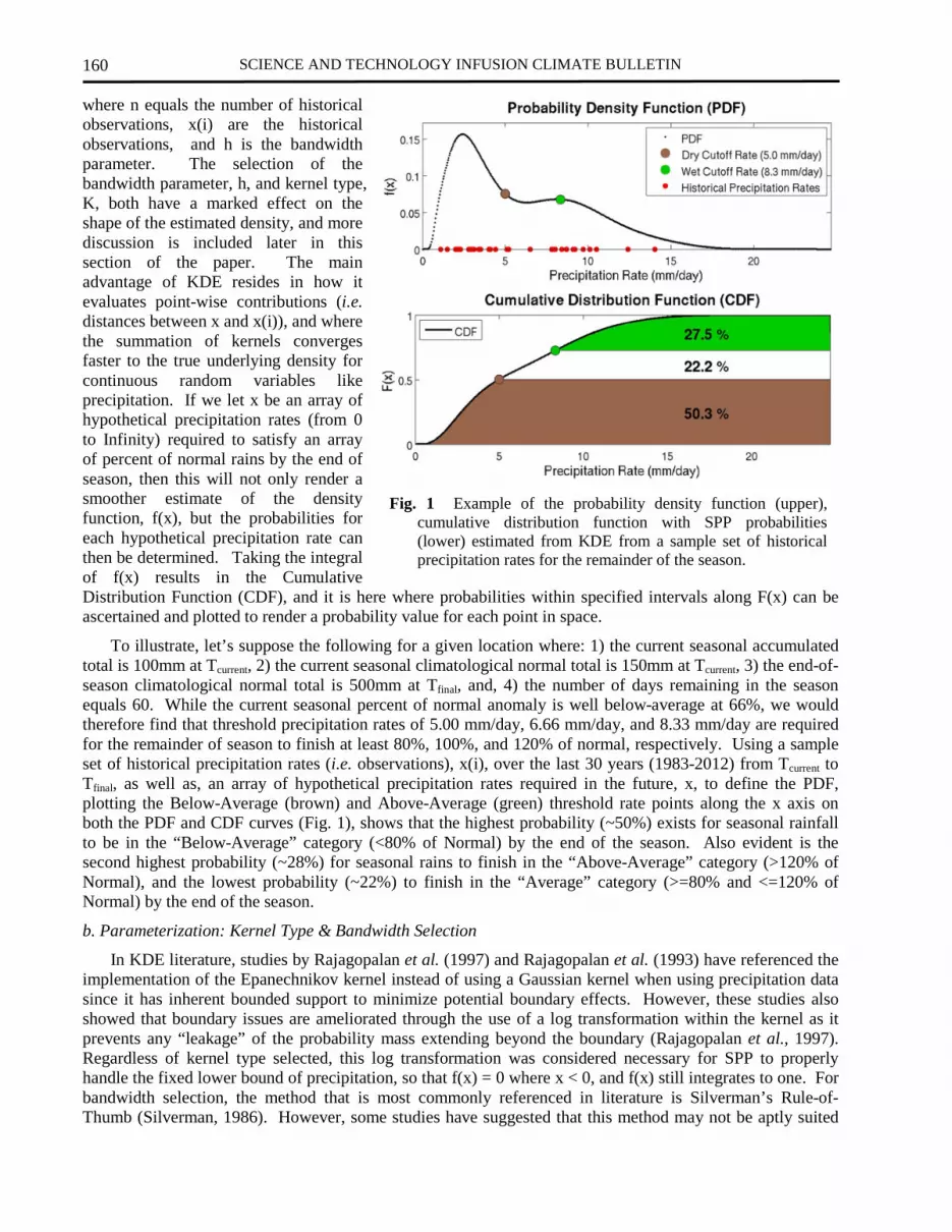
SCIENCE AND TECHNOLOGY INFUSION CLIMATE BULLETIN
160
where n equals the number of historical observations, x(i) are the historical observations, and h is the bandwidth parameter. The selection of the bandwidth parameter, h, and kernel type, K, both have a marked effect on the shape of the estimated density, and more discussion is included later in this section of the paper. The main advantage of KDE resides in how it evaluates point-wise contributions (i.e. distances between x and x(i)), and where the summation of kernels converges faster to the true underlying density for continuous random variables like precipitation. If we let x be an array of hypothetical precipitation rates (from 0 to Infinity) required to satisfy an array of percent of normal rains by the end of season, then this will not only render a smoother estimate of the density function, f(x), but the probabilities for each hypothetical precipitation rate can then be determined. Taking the integral of f(x) results in the Cumulative Distribution Function (CDF), and it is here where probabilities within specified intervals along F(x) can be ascertained and plotted to render a probability value for each point in space.
To illustrate, let’s suppose the following for a given location where: 1) the current seasonal accumulated total is 100mm at Tcurrent, 2) the current seasonal climatological normal total is 150mm at Tcurrent, 3) the end-of-season climatological normal total is 500mm at Tfinal, and, 4) the number of days remaining in the season equals 60. While the current seasonal percent of normal anomaly is well below-average at 66%, we would therefore find that threshold precipitation rates of 5.00 mm/day, 6.66 mm/day, and 8.33 mm/day are required for the remainder of season to finish at least 80%, 100%, and 120% of normal, respectively. Using a sample set of historical precipitation rates (i.e. observations), x(i), over the last 30 years (1983-2012) from Tcurrent to Tfinal, as well as, an array of hypothetical precipitation rates required in the future, x, to define the PDF, plotting the Below-Average (brown) and Above-Average (green) threshold rate points along the x axis on both the PDF and CDF curves (Fig. 1), shows that the highest probability (~50%) exists for seasonal rainfall to be in the “Below-Average” category (<80% of Normal) by the end of the season. Also evident is the second highest probability (~28%) for seasonal rains to finish in the “Above-Average” category (>120% of Normal), and the lowest probability (~22%) to finish in the “Average” category (>=80% and <=120% of Normal) by the end of the season.
b. Parameterization: Kernel Type & Bandwidth Selection
In KDE literature, studies by Rajagopalan et al. (1997) and Rajagopalan et al. (1993) have referenced the implementation of the Epanechnikov kernel instead of using a Gaussian kernel when using precipitation data since it has inherent bounded support to minimize potential boundary effects. However, these studies also showed that boundary issues are ameliorated through the use of a log transformation within the kernel as it prevents any “leakage” of the probability mass extending beyond the boundary (Rajagopalan et al., 1997). Regardless of kernel type selected, this log transformation was considered necessary for SPP to properly handle the fixed lower bound of precipitation, so that f(x) = 0 where x < 0, and f(x) still integrates to one. For bandwidth selection, the method that is most commonly referenced in literature is Silverman’s Rule-of-Thumb (Silverman, 1986). However, some studies have suggested that this method may not be aptly suited
Fig. 1 Example of the probability density function (upper), cumulative distribution function with SPP probabilities (lower) estimated from KDE from a sample set of historical precipitation rates for the remainder of the season.

NOVELLA AND THIAW
161
for mutli-modal distributions, and underperformance has been linked to its heavy reliance to assumptions of the underlying distribution (Rajagopalan et al., 1997). As an alternative, the “plug-in” or recursive method of (Sheather and Jones, 1991) (hereafter referred to as SJ) has also been widely described in KDE associated literature. In light of all findings related to the kernel type and bandwidth methods, log transformed Gaussian and Epanechnikov kernels, as well as, the Silverman and SJ bandwidth methods were evaluated in verification analysis to determine optimality for SPP in the following section.
3. Results
a. Historical reprocessing and verification
In determining the optimal KDE parameters for SPP in operational monitoring, the SPP algorithm was reprocessed using kernels and bandwidth methods, as highlighted in the previous section, over several key monsoonal periods and regions in eastern, southern and western Africa from 2010 to 2014. No reprocessing prior to 2010 was performed, since SPP still requires a high number of years to generate densities. For this exercise, verification consisted of calculating the Heidke Hit Proportion (HHP) scores for probabilistic forecasts (IRI, 2013). This verification metric was regarded as the most straight-forward and relevant in forecasting anomaly categories corresponding to below-average, average, and above-average seasonal rainfall. HHP awards credit (hits) where the highest categorical SPP probability matches the observed category by the end of season. Hits are then summed and divided by the total number of forecasts in space.
Averaged HHP scores (from 2010-2014) using various parameterizations in SPP for all seasons and regions in shown in Table 1. The most salient observation is that there doesn’t appear to be any distinct advantage in using a particular kernel, or a particular bandwidth method in terms of improved HHP verification scores, since differences in HHP scores between kernel types and bandwidth methods appear to be quite negligible at seasonal stages. By the end of the first month and through mid-point of each season, HHP scores range between 0.6 and 0.7 indicating that at least 60% of the SPP probability fields correctly verified in their respective anomaly category. While not perfect, these scores suggest a level of confidence for operational monitoring, where we can provide reasonable guidance of a seasonal rainfall outcome to users before halfway through the season. Based on these results, the Gaussian kernel and Silverman’s bandwidth method was selected for operational SPP implementation purely due their efficiency in daily processing.
b. SPP case studies
Perhaps the most well-known drought case study in recent years was the severe drought that devastated East Africa from 2010-2011. In our monitoring of precipitation, ARC2 accurately depicted the onset of the drought during the Oct-Dec rainfall season, and captured the extent of worsening dryness conditions due to poor rains during the following March-May rainfall season in the same region (Novella and Thiaw, 2013). Figs. 2a-d show the reprocessed SPP for the Oct-Dec, 2010 rainfall season in East Africa. After one month (1/3) into the season,
Table 1 Averaged HHP scores from 2010-2014 using various KDE parameterizations in SPP for all seasons and regions (h1=Silverman, h2=SJ).

SCIENCE AND TECHNOLOGY INFUSION CLIMATE BULLETIN
162
the percent of normal ARC2 rainfall on November 1st, 2010 (Fig. 2a) begins to depict developing dryness throughout much southern Somalia, southwestern Ethiopia, eastern Kenya, and across much of Tanzania. For areas that experienced rapidly developing dryness, SPP probabilities are highest in the below-average category (Fig. 2c), with 80% to 90% probabilities over areas where climatologically, lesser amounts of rainfall are expected for remainder of season, thus reflecting the increased likelihood of drought development and persistence before the end of the season. Analysis of the final season percent of normal rainfall (Fig. 2b) and HHP verification score map (Fig. 2d) on November 1st, 2010 indicate that nearly 70% of the seasonably active areas in east Africa had SPP probabilities that correctly verified in the respective anomaly categories.
In a more recent case study, the core of the southern Africa rainy season, Dec, 2014 – Feb, 2015 has been characterized as being poor and highly erratic. This had presented a greater challenge to SPP during operational monitoring due to unusual reversals in the monsoon circulation that had been observed throughout the course of the season. By the end of February, a dipole anomaly pattern emerged with the southeastern portion of the Africa continent having experienced well above-average rainfall, and below-average moisture conditions prevailing throughout much of southwestern Africa (Fig. 3a). However, the evolution of this dipole was not straight-forward nor gradual as one might expect. In the middle of December, much of southeastern Africa (i.e. eastern Zambia, Malawi, and western Mozambique) had experienced a delayed onset of the monsoon, raising concerns of anomalous dryness persisting into the season. SPP probabilities for below-average Dec-Feb rainfall began to increase and expand throughout the region, until extreme rains fell in late December, which led to an abrupt reversal in the SPP probabilities between the above and below average anomaly categories. By early January 2015, SPP probabilities over much of southern Angola, northern Namibia and the Caprivi Strip did not correctly verify as being below-average. Only after an extended dry spell had transpired during January in the region did SPP point to a high probability for below-average rains by the end of the season. In Figs. 3c-d, we see the SPP probabilities and HHP hit map illustrating nearly 70% of the seasonably active areas in southern Africa had SPP probabilities that correctly verified in the respective anomaly categories by January 15th.
c. SPP real-time operational output
Consistent with the real-time, daily maps and time series products updated at CPC, the SPP algorithm consists of generating probabilistic output for every gridded pixel, every day over Africa. In an effort to
a b
c d
Fig. 2 East Africa spatial maps of (a) percent of normal seasonal rainfall anomaly on Nov 1st, 2010, (b) the final percent of normal seasonal rainfall anomaly captured Dec 31st, 2010, (c) SPP reprocessed on Nov 1st, 2010, (d) Heidke Hit Proportion (HHP) of verified hits (green) and misses (red) on Nov 1st, 2010.

NOVELLA AND THIAW
163
further relax an intense computational environment, the resulting SPP spatial fields are aggregated from a 0.1° to 0.25° resolution. To best cover the seasonality of precipitation over Africa, users will be able to choose any base period spanning 1 to 4 months of ARC2 accumulated rainfall, and a probabilistic outlook period ranging from the end of the current month out to 3 months. SPP output consists of single map depicting all probabilities corresponding to Below-Average (<80% of Normal), Average (>=80% and <=120% of Normal), and Above-Average (>120% of Normal) rainfall for the end of every projection period.
4. Conclusions
This paper describes a new statistical tool, called SPP, which computes spatial probability maps for seasonal precipitation to finish at rainfall anomaly categories corresponding to Below Average (<80% of normal), Average (80-120% of normal), and Above-Average (>120% of normal) over Africa. These computations are achieved through the use of Kernel Density Estimation (KDE) methods which yield probability density functions (PDF’s) and cumulative density functions (CDF’s) based on 30+ years of historical ARC2 precipitation for the remaining duration of a monsoon season. The daily, real-time availability of ARC2 used in operational monitoring also permits SPP output to be disseminated to users on the same basis.
Reprocessing and verification results indicate that, on average, at least 60% of the SPP probability fields had correctly verified in their respective anomaly category. This suggests there is a reliable degree of confidence in SPP for providing the outcome of seasonal rainfall during operational monitoring. Such information is expected to translate into better decision making in food security, planning and response objectives for USAID/FEWS-NET.
References
Novella, N., W. Thiaw, 2013: Africa rainfall climatology version 2 for Famine Early Warning Systems. Journal for Applied Meteorology and Climatology, 52, 588-606.
Rajagopalan, B., U. Lall, D.G. Tartoton, 1993: Simulation of daily precipitation from a nonparametric renewal model. Utah State University Digital Commons Reports Paper 146.
Rajagopalan, B., U. Lall, D.G. Tartoton, 1997: Evaluation of kernel density estimation methods for daily precipitation resampling. Stochastic Hydrology and Hydraulics, 11, 523-547.
Sheather, S.J., M.C. Jones, 1991: A reliable data-based bandwidth selection method for kernel density estimation. Journal of the Royal Statistical Society, Series B. 53, 683-690.
Silverman, B.W., 1986: Density estimation for statistics and data analysis. Chapman and Hall, New York.
Fig. 3 Southern Africa spatial maps of (a) percent of normal seasonal rainfall anomaly on Jan 15th, 2015, (b) the final percent of normal seasonal rainfall anomaly captured Feb 28th, 2015, (c) SPP reprocessed on Jan 15th, 2015, (d) Heidke Hit Proportion (HHP) of verified hits (green) and misses (red) on Jan 15th, 2015.
a b
c d

APPENDIX :
WORKSHOP PHOTOS
40th NOAA Climate Diagnostics and Prediction Workshop


NWS Science and Technology Infusion Climate Bulletin
Featured Special Collections (http://www.nws.noaa.gov/ost/climate/STIP/Collections.htm)
Climate Prediction Science and Technology Digest
1. 39th Climate Diagnostics and Prediction Workshop
2. 38th Climate Diagnostics and Prediction Workshop
3. 37th Climate Diagnostics and Prediction Workshop
4. 36th Climate Diagnostics and Prediction Workshop
5. 35th Climate Diagnostics and Prediction Workshop
6. 34th Climate Diagnostics and Prediction Workshop
7. 33rd Climate Diagnostics and Prediction Workshop
NOAA Climate Test Bed Joint Seminar Series Extended Summaries Collection Volume
1. Unified Modeling, Seamless Prediction and Integrated Services (2010-2011)
2. Assessment of Improvement in Climate Prediction with Outstanding R&D Needs (2009-2010)
3. Research to Operation and Operation to Research (2008-2009)
4. CFS as a Prediction System and Research Tool (2007-2008)
S&T Infusion Lecture Series & Notes
1. Notes about CPC’s seasonal prediction
2. Uncertainty and Ensemble Forecast