Int. J. Environment and Pollution, 1

Copyright © 1997 Inderscience Enterprises Ltd.

Combined use of space-borne observations of NO2 and regional CTM model for air quality monitoring in Northern Italy

Petritoli A.1, E. Palazzi1, G. Giovanelli1, W. Di Nicolantonio2, G. Ballista2, C. Carnevale3, G. Finzi3, E. Pisoni3*, M. Volta3

1Institute of Atmospheric Science and Climate, ISAC-CNR, via P. Gobetti 101, 40129, Bologna, Italy 2Carlo Gavazzi Space at ISAC-CNR, via P. Gobetti 101, 40129, Bologna, Italy 3Department of Electronics for Automation, University of Brescia, Italy

*Corresponding author

Abstract: The use of space-borne measurements of trace gas constituents for

air quality monitoring has considerably increased during the past decade. This

is mainly due to the new generation sensors able to observe large areas with

good temporal resolution and due to new assimilation techniques that allow a

synergetic use of information from satellite and from Chemical Transport

Models (CTM). In this paper we present the work that has been performed so

far within the QUITSAT project, funded by the Italian Space Agency.

SCIAMACHY observations of earth radiance are used to retrieve NO2

tropospheric column by DOAS spectrometric technique and radiative transfer

modelling for AMF computation. These satellite column measurements of

nitrogen dioxide are then merged with the simulations of the Transport

Chemical Aerosol Model (TCAM) to improve the model output at the ground

level. The method used is a weighted rescaling of the model column in the

troposphere according to the SCIAMACHY observations where the weights

are the measurement errors and the model column variances within the satellite

ground-pixel, respectively. The employed data are related to the Northern Italy

2 Book reviews

area. The obtained ground concentrations of NO2 have been compared with in-

situ observations performed by the regional Environmental Agencies. Results

show good agreement mainly where well horizontal mixing is present.

Keywords: EOS data, Chemical Transport Models, NO2.

Biographical notes: Andrea Petritoli collaborates with ISAC-CNR institute on

atmospheric trace gases monitoring with DOAS technique and its applications on

air quality and climatic issues. He is Ph.D. in atmospheric science.

Elisa Palazzi has a post-doctoral fellowship at ISAC-CNR. She is experienced

with the development of radiative transfer models for the interpretation of

passive and active remote sensing measurements.

Giorgio Giovanelli is a senior scientist at ISAC-CNR. He has more than 30

years of experience on atmospheric remote sensing observations of trace gases.

His main research interest now is on advanced DOAS spectroscopy.

W. Di Nicolantonio joined Carlo Gavazzi Space (CGS) in Milan, Italy, in

1998. From 2002 he is in charge of Bologna division of CGS Earth

Observation and Application Department.

G. Ballista develops systems for Earth Observation data processing. In

particular he performs analysis related to NRT data acquisition and data

processing for the Seviri radiometer.

C. Carnevale, is an assistant professor at the University of Brescia. His

research fields include modelling and control of environmental systems, system

identification, nonlinear programming.

G. Finzi is full professor of Automatic Control at f the University of Brescia.

She works on environmental control and management in the frame of national

Book reviews 3

and international scientific projects.

Enrico Pisoni is an assistant professor at University of Brescia. His research

interests include modelling and simulation of non linear systems, system

identification and optimization techniques.

M. Volta is an associate professor of Automatic Control at University of

Brescia. Her research interests include modelling and control of dynamic

systems, system identification, decision support systems.

1 Introduction

Satellite-borne observations of tropospheric trace gases composition has been

widely used for different kind of atmospheric research issues: from climatic

considerations (Richter et al., 2005) to air pollution monitoring (Wenig et al.,

2003). Their main positive characteristics are global coverage and fair spatial

resolution but still remain strong limitation in time resolution and requirements

for the atmospheric conditions during measurement (mainly for the small cloud

coverage and low aerosol loading). As a matter of fact from the work of Richter

and Burrows (2002), which firstly gave a look at tropospheric pollution problem

from a global point of view, satellite observations of trace constituents seem to

deserve a consistent role in the study and monitoring of air pollution.

But one of the main problem that satellite observations have to face in order to be

used in air quality assessment is the unknown of pollutants vertical distribution.

In fact the only information we can obtain from space-borne instruments

concerning the troposphere is column abundance, i.e. the concentration of the

4 Book reviews

trace constituent integrated along the vertical direction. Such measurements

cannot always distinguish between pollution transported from other places and

then located presumably in the free troposphere and pollution at lower level that

can be in direct contact with population. So if the spatial resolution as well as the

time resolution have been improved from GOME (Burrows et al., 1999) on ERS-

2 to OMI (Veefkind et al., 2006) on AURA through SCIAMACHY

(Bovensmann et al., 1999) on ENVISAT, the information on the vertical resolved

profile of concentration in the lower troposphere cannot be easily solved without

a new approach to measurement geometry and/or inversion techniques. For this

reason the integration with other tools is required. Assimilation of satellite

observations into Chemical and Trasport Models (CTM) is a possible solution

that has been already used mainly for stratospheric measurements (Lahoz et al,

2007 ) and with different purposes not connected to air pollution monitoring.

Ground based measurements have been used so far for this scope instead (Elbern

e al, 2001) but one of the advantages of satellite data is that its spatial resolution

is similar to that of a CTM working on a regional scale, and its coverage is

usually homogeneous over the considered domain.

What we propose in this paper are the results of a research work performed

within the QUITSAT project, funded by the Italian Space Agency (ASI), and

focused on the combined use of satellite data and CTM simulations to improve

the monitoring of trace gases concentrations at ground level. Our work is based

on the observations of nitrogen dioxide (NO2) provided by the SCIAMACHY

sensor on board ESA ENVISAT platform and model simulations obtained from

Book reviews 5

TCAM model (Carnevale et. al, 2008). In the subsequent sessions we present

briefly the developed methodology, the results obtained in terms of NO2

concentrations at ground levels and the validation of the method by means of

comparison with ground-based measurements performed by the regional

environmental agencies. A more detailed analysis of the proposed methodology

and of the application results, is presented in the work of Di Nicolantonio et al

(2009).

2 Methodology

One of the aim of the QUITSAT project is to provide a prototype system to

monitor air pollution also in terms of ground concentrations of main trace gases

pollutants such as nitrogen dioxide; that is to say to have a near real time analysis

in the considered domain. We used for this scope SCIAMACHY data and TCAM

simulations both described in the following subsections as well as the merging

method we have developed.

2.1 Satellite data

The primary objective of the SCanning Imaging Absorption SpectroMeter for

Atmospheric CHartographY (SCIAMACHY) mission is to perform global

measurements of trace gases in the troposphere and in the stratosphere

(Bovensmann et al., 1999). The solar radiation transmitted, backscattered and

reflected from the atmosphere is recorded at relatively high resolution (0.2 nm to

0.5 nm) over the range 240 nm to 1700 nm, and in selected regions between 2000

6 Book reviews

nm and 2400 nm with different viewing geometries: nadir, limb, and sun/moon

occultation. In this work we used only nadir observations in the UV-Vis spectral

region to obtain the nitrogen dioxide slant column through the DOAS

(Differential Optical Absorption Spectroscopy) technique (Platt, 1999). The

stratospheric contribution to the total column is removed according to the method

proposed by Richter and Burrows (2002) and the obtained tropospheric slant

column is converted into tropospheric vertical column using the Air Mass Factor

calculated with the PROMSAR model (Palazzi et al., 2005). The satellite ground

pixel extension can be different depending on the measurements mode: in the 400

nm spectral region at mid-latitudes its dimension is about 30x60 km2 and the

overpass time is at 10:30 am Local Time. As briefly mentioned above one of the

most important limitation of this kind of remote sensing measurements in the

UV-Visible part of the solar spectrum is the influence of clouds in the

instrumental field of view. In this case the interpretation of the observed signal is

too complicated and usually ground pixel with cloud cover greater than few

percent are removed from the analysis.

2.2 Chemical Transport Model simulations

GAMES modelling system (Volta et al., 2006) has been used in this study. The

system harmonizes three main modules: (a) the multi-phase Eulerian 3D

photochemical model TCAM (Transport Chemical Aerosol Model, (Carnevale et

al., 2008); (b) the meteorological pre-processor PROMETEO; (c) the emission

processor POEMPM (Carnevale et al., 2008) specifically designed to produce

present and alternative emission scenarios. In this study GAMES has been

Book reviews 7

applied over an area covering the entire Po Valley. The domain (640 km × 480

km) has been horizontally subdivided into 64x48 cells, with a resolution of 10

km × 10 km each. Vertical domain extends up to 3900 m a.g.l., and is subdivided

into 11 layers of growing thickness. Simulations have been performed getting

initial and boundary conditions by a nesting procedure from the results of

CHIMERE simulations over Europe. The point sources and area emissions have

been chemically and temporally adjusted to TCAM requirements and have been

derived by CTN-ACE Italian modelling intercomparison project (Deserti et. al.,

2009). Meteorological fields have been created with MM5 model and adapted to

TCAM through PROMETEO pre-processor. With these features, the base case

simulation (year 2004) has been simulated and validated in the frame of

QUITSAT project. In this work TCAM NO2 ground concentrations have been

extracted, at satellite passing hours, to be integrated with SCIAMACHY

measurements.

2.3 Merging the two data

The approach we have followed to merge satellite data with model simulation

was aimed by a time saving goal and by the fact that satellite data

(SCIAMACHY in particular) have still a low temporal resolution to be

assimilated in a regional model. The only advantage we can have is in terms of

ground concentration at the satellite overpass. At this time we can merge space-

borne column measurements and CTM 3D runs to improve the accuracy of the

8 Book reviews

trace gas ground concentrations simulated by the model. This is done according

to the following steps:

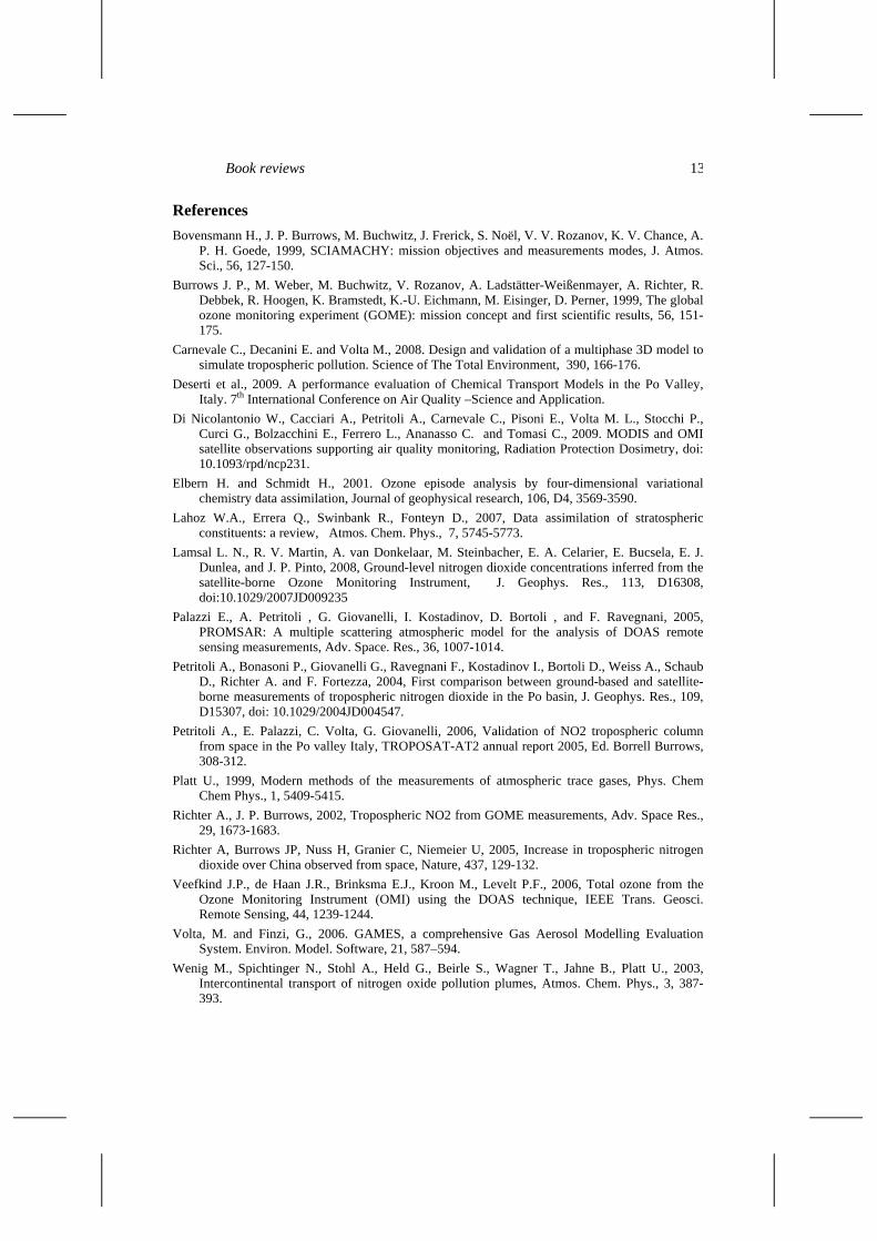
i) The NO2 tropospheric column from satellite (CS) and its error (CS)

are estimated using DOAS technique;

ii) Similar quantities are obtained from the model (CM and CM) by

integrating the vertical profile to get the tropospheric columns (the

model vertical extension is up to 4 km a.g.l). All the CM whose

central latitude and longitude match the satellite ground pixel area

are then averaged to get the final CM and CM is its variance (see

Figure 1).

iii) A corrected column (CC) is thus calculated using CM and CS

according to the following formula

M

M

S

S

M

M

S

S

C

C

C

C

C

C

C

C

C

C

22

that is CC is a weighted average between CM and CS where the

respective errors are the weights;

iv) An average NO2 profile corresponding to the satellite ground pixel is

calculated from the model simulations and the respective column is

scaled so to be equal to CC obtaining then a corrected profile. The

Ground Level concentration thus Corrected is considered our final

product (GLCNO2).

Book reviews 9

The goal of the weighted average at step (iii) is to give more importance to the

more reliable columns values. As we can argue from Figure 1 the SCIAMACHY

ground pixel contains several TCAM cells. So we decided to chose the CM

variances as its errors since it is a rough estimation of the possible variability of

NO2 modeled column within the SCIAMACHY pixel. The final results of our

approach is thus to rescale the model profiles using the satellite observations: a

similar method, with different scaling scheme, has been proposed by Lamsal et

al. (2008) on OMI data.

3 Case study application

The method explained in the previous section has been used to get GLCNO2

concentrations during 2004 in the Po valley region that is the target area to

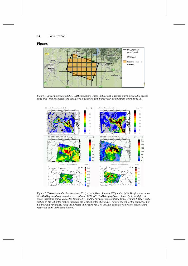
investigate within the QUITSAT project. In Figure 2 we present two case studies

for November 20th (on the left part of the Figure) and January 28th (on the right

part of the Figure). The first row contains the respective concentration at ground

level simulated with TCAM at 10 am LT, the second one the NO2 tropospheric

column as obtained by the SCIAMACHY sensor and the third one the GCLNO2

concentration (see step iv in the previous section).

Concerning the November 20th we can see immediately a similar pattern

between the first two rows meaning that probably great part of the NO2 observed

and simulated is located in the lowest troposphere. This does not seem to be

completely true for the January 28th when over Piemonte, Liguria and Mar

10 Book reviews

Ligure (the western part of Italy represented in the map) TCAM reports low NO2

at the ground level while the column from SCIAMACHY is remarkably high

(this actually makes sense if NO2 was located at higher levels). In the other parts

of Po valley the patterns look similar. The third row of Figure 2 gives the

GLCNO2 for both considered days respectively. The pattern could be different

from those of TCAM and SCIAMACHY (see November 20th) but also similar

(January 28th) depending on the vertical distribution of NO2 and on the relative

weights of CS and CM (see above).

In order to validate the GLCNO2 concentration we have compared the obtained

values with simultaneous measurements performed in situ by the regional

environmental agency (ARPA) from Emilia Romagna and Lombardia regions

(see Petritoli et al., 2004 for more details on ARPA measurements). Of course the

comparison between an in situ sampling and the GLCNO2 values that is referred to

a 30km x 60km regions could be misleading. But this is not the case if we know

what we could expect from the comparison. In previous works (Petritoli et al.,

2004 and Petritoli et al., 2005) we have treated similar situations concluding that

satellite measurements (and derived measurements as GLCNO2) give different

information from in situ sampling as far as their spatial resolution will remain as

large. Both observations can be homogeneous (thus comparable) if the air mass

sampled by satellite is well mixed otherwise space-borne measurements will

represent an average of the trace constituents in the observed area that in general

is different from the in situ sampling at ground stations.

Book reviews 11

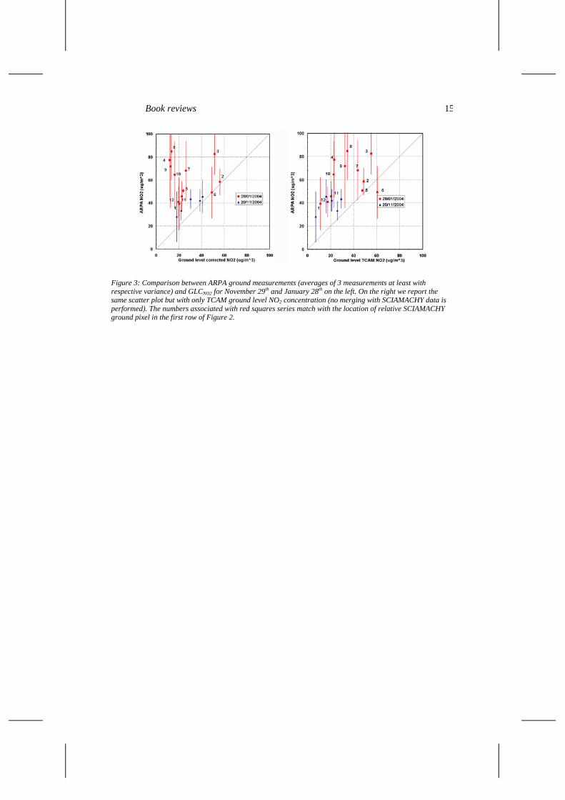
In Figure 3 the comparison between GLCNO2 and ARPA observations is shown

on the left. Only ground pixel where at least 3 ARPA observations were available

have been chosen and their averages are calculated to be compared with GLCNO2.

The respective variances are shown as error bars in the plot. November 20th data

show good agreement (correlation coefficient R= 0.85) and low variance in

ARPA measurements. This could be probably connected with good horizontal

mixing as explained above. We have a different situation on the January 28th.

Only few data are comparable (ground pixels 2 and 6 for which we notice also

that the measurements weight are relevant: in fact Figure 2 shows how model

simulations gives higher concentration in location 6 than 2 while GLCNO2 are

reversed) and in particular ground pixels 3,4,7,8,9,10 show large variances and

bad correlation. Again this seems to fit our previous reasoning on the horizontal

mixing of the sampled air masses. Also the pattern of NO2 ground concentration

from TCAM (Figure 2, first row) reveals possible high gradients in the nearby of

the areas occupied by the above pixels.

The plot of Figure 3 (right) shows a similar comparison between ARPA and only

TCAM NO2 ground concentration calculated within the respective

SCIAMACHY ground pixel so to estimate the contribution of the SCIAMACHY

measurements to the GLCNO2. On the November 11th all the data benefits of the

correction while on the January 28th only few ground pixels (1,2,6) seems to

improve their correlation. This is consistent anyway with the previous

explanation of a no efficient horizontal mixing during this day with the

consequent presence of sharp gradients in NO2 concentration.

12 Book reviews

4 Conclusions

Satellite-borne observations of air pollution have great potentiality to be used

together with CTM models to monitor air quality also at ground level. In this

work we have shown a possible merging of SCIAMACHY NO2 observations

with the TCAM CTM regional model. The presented method is fast (suitable

then to be used for near real time monitoring) and give fair results in terms of

representativeness of the ground level corrected NO2 concentrations (GLCNO2) as

shown by the comparison with ARPA measurements. Other space borne sensors

have already improved the limitation of SCIAMACHY (like OMI with better

time and spatial resolution) and even better projects are going to be developed in

the near future. Considering also the high costs of maintenance of ground

instrumentations this synergy is a promising road to follow for air quality science

and monitoring.

Acknowledgments

The authors would like to thank ARPA Emilia Romagna and ARPA Lombardia

for providing in situ measurements and CETEMPS (University of L’Aquila) for

the initial and boundary conditions from CHIMERE simulations. The research

has been developed in the framework of the Pilot Project QUITSAT (QUalità

dell’aria mediante l’Integrazione di misure da Terra, da SAtellite e di

modellistica chimica multifase e di Trasporto - contract I/035/06/0 –

http://www.quitsat.it), sponsored and funded by the Italian Space Agency (ASI).

Book reviews 13

References

Bovensmann H., J. P. Burrows, M. Buchwitz, J. Frerick, S. Noël, V. V. Rozanov, K. V. Chance, A. P. H. Goede, 1999, SCIAMACHY: mission objectives and measurements modes, J. Atmos. Sci., 56, 127-150.

Burrows J. P., M. Weber, M. Buchwitz, V. Rozanov, A. Ladstätter-Weißenmayer, A. Richter, R. Debbek, R. Hoogen, K. Bramstedt, K.-U. Eichmann, M. Eisinger, D. Perner, 1999, The global ozone monitoring experiment (GOME): mission concept and first scientific results, 56, 151-175.

Carnevale C., Decanini E. and Volta M., 2008. Design and validation of a multiphase 3D model to simulate tropospheric pollution. Science of The Total Environment, 390, 166-176.

Deserti et al., 2009. A performance evaluation of Chemical Transport Models in the Po Valley, Italy. 7th International Conference on Air Quality –Science and Application.

Di Nicolantonio W., Cacciari A., Petritoli A., Carnevale C., Pisoni E., Volta M. L., Stocchi P., Curci G., Bolzacchini E., Ferrero L., Ananasso C. and Tomasi C., 2009. MODIS and OMI satellite observations supporting air quality monitoring, Radiation Protection Dosimetry, doi: 10.1093/rpd/ncp231.

Elbern H. and Schmidt H., 2001. Ozone episode analysis by four-dimensional variational chemistry data assimilation, Journal of geophysical research, 106, D4, 3569-3590.

Lahoz W.A., Errera Q., Swinbank R., Fonteyn D., 2007, Data assimilation of stratospheric constituents: a review, Atmos. Chem. Phys., 7, 5745-5773.

Lamsal L. N., R. V. Martin, A. van Donkelaar, M. Steinbacher, E. A. Celarier, E. Bucsela, E. J. Dunlea, and J. P. Pinto, 2008, Ground-level nitrogen dioxide concentrations inferred from the satellite-borne Ozone Monitoring Instrument, J. Geophys. Res., 113, D16308, doi:10.1029/2007JD009235

Palazzi E., A. Petritoli , G. Giovanelli, I. Kostadinov, D. Bortoli , and F. Ravegnani, 2005, PROMSAR: A multiple scattering atmospheric model for the analysis of DOAS remote sensing measurements, Adv. Space. Res., 36, 1007-1014.

Petritoli A., Bonasoni P., Giovanelli G., Ravegnani F., Kostadinov I., Bortoli D., Weiss A., Schaub D., Richter A. and F. Fortezza, 2004, First comparison between ground-based and satellite-borne measurements of tropospheric nitrogen dioxide in the Po basin, J. Geophys. Res., 109, D15307, doi: 10.1029/2004JD004547.

Petritoli A., E. Palazzi, C. Volta, G. Giovanelli, 2006, Validation of NO2 tropospheric column from space in the Po valley Italy, TROPOSAT-AT2 annual report 2005, Ed. Borrell Burrows, 308-312.

Platt U., 1999, Modern methods of the measurements of atmospheric trace gases, Phys. Chem Chem Phys., 1, 5409-5415.

Richter A., J. P. Burrows, 2002, Tropospheric NO2 from GOME measurements, Adv. Space Res., 29, 1673-1683.

Richter A, Burrows JP, Nuss H, Granier C, Niemeier U, 2005, Increase in tropospheric nitrogen dioxide over China observed from space, Nature, 437, 129-132.

Veefkind J.P., de Haan J.R., Brinksma E.J., Kroon M., Levelt P.F., 2006, Total ozone from the Ozone Monitoring Instrument (OMI) using the DOAS technique, IEEE Trans. Geosci. Remote Sensing, 44, 1239-1244.

Volta, M. and Finzi, G., 2006. GAMES, a comprehensive Gas Aerosol Modelling Evaluation System. Environ. Model. Software, 21, 587–594.

Wenig M., Spichtinger N., Stohl A., Held G., Beirle S., Wagner T., Jahne B., Platt U., 2003, Intercontinental transport of nitrogen oxide pollution plumes, Atmos. Chem. Phys., 3, 387-393.

14 Book reviews

Figures

Figure 1: At each overpass all the TCAM simulations whose latitude and longitude match the satellite ground pixel area (orange squares) are considered to calculate and average NO2 column from the model (CM).

Figure 2: Two cases studies for November 20th (on the left) and January 28th (on the right). The first row shows TCAM NO2 ground concentrations, second row SCIAMACHY NO2 tropospheric columns (note the different scales indicating higher values for January 28th) and the third row represents the GLCNO2 values. S labels in the picture on the left of the first row indicate the location of the SCIAMACHY pixels chosen for the comparison of Figure 3 (blue triangles) while the numbers in the same rows on the right panel associate each pixel with the respective point in the same Figure 3.

Book reviews 15

Figure 3: Comparison between ARPA ground measurements (averages of 3 measurements at least with respective variance) and GLCNO2 for November 29th and January 28th on the left. On the right we report the same scatter plot but with only TCAM ground level NO2 concentration (no merging with SCIAMACHY data is performed). The numbers associated with red squares series match with the location of relative SCIAMACHY ground pixel in the first row of Figure 2.