Compliance for uncertain inventoriesvia probabilistic/fuzzy comparison of alternatives

Olgierd Hryniewicz & Zbigniew Nahorski &Jörg Verstraete & Joanna Horabik & Matthias Jonas

Received: 22 December 2012 /Accepted: 6 December 2013 /Published online: 15 February 2014# The Author(s) 2014. This article is published with open access at Springerlink.com

Abstract A direct comparison among highly uncertain inventories of emissions is inadequateand may lead to paradoxes. This issue is of particular importance in the case of greenhousegases. This paper reviews the methods for the comparison of uncertain inventories in thecontext of compliance checking. The problem is treated as a comparison of uncertain alterna-tives. It provides a categorization and ranking of the inventories which can induce compliancechecking conditions. Two groups of techniques to compare uncertain estimates are consideredin the paper: probabilistic and fuzzy approaches. They show certain similarities which arerevealed and stressed throughout the paper. The group of methods most suitable for thecompliance purpose is distinguished. They introduce new conditions for fulfilling compliance,depending on inventory uncertainty. These new conditions considerably change the presentapproach, where only the reported values of inventories are accounted for.

1 Introduction

A handful of solutions have been proposed to cope with the problem of emission commitmentevaluation for uncertain inventories, see Jonas and Nilsson (2007). Numerous propositionshave pointed to methodological incompetence in using the reported (point) values in clearingemission targets. For many environmental problems such as for greenhouse gases, only highlyimprecise values of emission are available, see e.g. Jonas and Nilsson (2007); Jonas et al.(2010b); Lieberman et al. (2007); White et al. (2011). Apart from a high uncertainty level,uncertainty distributions are often asymmetric, as they reflect non-negative measurements ofphysical quantities. For an example, see the results in Ramirez et al. (2006) or Winiwarter andRypdal (2001).

Climatic Change (2014) 124:519–534DOI 10.1007/s10584-013-1031-x

This article is part of a Special Issue on “Third International Workshop on Uncertainty in Greenhouse GasInventories” edited by Jean Ometto and Rostyslav Bun.

Electronic supplementary material The online version of this article (doi:10.1007/s10584-013-1031-x)contains supplementary material, which is available to authorized users.

O. Hryniewicz : Z. Nahorski (*) : J. Verstraete : J. HorabikSystems Research Institute, Polish Academy of Sciences, Newelska 6, 01-447 Warsaw, Polande-mail: Zbigniew.Nahorski@ibspan.waw.pl

M. JonasInternational Institute for Applied Systems Analysis, Schlossplatz 1, 2361 Laxenburg, Austria

According to the IPCCGood Practice Guidelines (IPCC 1996), a report should be “consistent,comparable and transparent”. Decisions on the fulfilment of obligations should be fair for allparties, which means that it should be transparent why some inventories comply with commit-ments while others do not. Since greenhouse gases inventories are highly uncertain, makingdecisions on compliance or comparison of inventories based only on the reported values(estimated size) may contradict any conclusions inferred from considering uncertainty distribu-tions such as uncertainty range (e.g. standard deviation) and the shape of uncertainty distribution(e.g. skewness). We argue that this knowledge should be fully utilized to make decisions oncompliance and to infer a comparison of emissions.

Let us consider two uncertain emission inventories, A and B of Fig. 1a–b, whichwill help us to illustrate the techniques discussed. For the sake of simplicity, let usassume that both involved parties have the same emission limits, also called a target,for instance, an allocated number of emission permits. The dominant values of theuncertainty distribution densities μ(x) reflect the reported inventories of both parties,which are very close. If uncertainty is ignored, party A would be considered compli-ant (fulfilling the limit), while party B would not. However, confidence in the inventoryvalue of party B is high, while that of A is low, raising the question which party is morecredible? Should party A be considered compliant, while party B should not? Certainly, tocompare parties with different scale of emissions, the inventories have to be normalized. Forexample, the value d=(x−K) /x, with K denoting the party’s emission limit, may be a suitablenormalization; then the normalized limit is equal to zero. Henceforth, the term inventory willalways refer to a normalized inventory.

Fig. 1 Illustration for statistical approaches: a Comparison of means and variances; b Calculation of criticalvalues; c Illustration of compliance in the undershooting approach; d Stochastic dominance criterion forcomparison of inventories A and B; e The indecision interval

520 Climatic Change (2014) 124:519–534

In this paper we look at the problem of fulfillment as one of the comparison and ordering of(normalized) inventories. When inventories can be ordered in a transparent way, then we canpoint to the threshold value, below which the inventories are compliant, and above which theyare not. With the present method inventories care actually ordered according to the reportedvalues. Those which are below the limit are considered compliant, while those above are not.As mentioned before, the ordering of uncertain inventories simply according to their reportedvalues is dubious, since their uncertainty should also be taken into account. The idea of thispaper is to review the methods for comparison of uncertain values, so that uncertain invento-ries can be credibly ordered. This will introduce transparency into the compliance mechanism.Henceforth, a higher ranked inventory A is considered better in respect to (i.r.t.) the target thaninventory B, and is denoted by B≺A.

Verification of emission reduction in a single country may also face the problem ofuncertainty. Let us consider the case of greenhouse gases, when a reduction of emissions atthe end of the commitment period is required. This is expressed as a specified rate ρ of the realemissions in the previous (basic) year. Since the real emissions are not known, only anuncertain inventory in the compliance year, xc, can be compared with a reduced uncertaininventory in the basic year, ρxb. From this, it has to be decided whether the former emissionsare lower than the latter. In other words, these two inventories should be ranked in asconvincing a manner as possible. This also motivated our search for adequate methods tocompare uncertain values. But another view is also possible in this case. Consider a variabledefined as d ¼ xc

xb− ρ or the so called trend uncertainty d ¼ xb−xc

xb− 1−ρð Þ . These are

normalized variables, which can be used for comparison among countries with different scalesof emissions, and even with different reduction rates ρ. For them, the limit for comparisonequals zero. Consequently, countries can be ordered appropriately according to their values ofd and accounting for uncertainty. With this ordering, compliance conditions can be formulated.Note that for the Monte Carlo simulation, which is presently the basic tool for assessment ofuncertainty distributions, there is no great difference as to whether a distribution of variable dinstead of variable x is to be generated.

Nevertheless, it should be stressed that ranking is only supplementary to the compliancechecking rule that is adopted. It can help to justify why some inventories are consideredcompliant, while others are not. Ranking of inventories may facilitate avoiding paradoxicalsituations, when decisions on compliance or noncompliance are at variance with commonsense.

Throughout the paper it is assumed that the distribution of inventory uncertainty isavailable. This would be the ideal case. Unfortunately, for national GHG inventories it islargely impossible to estimate distributions in the statistical sense, since inventories cannotbe repeated in great numbers with different values of unsure parameters. The distributionscan be, however, assessed by performing Monte Carlo calculations, which provide goodinsight to the distribution of national inventories. Some countries (e.g. Austria, theNetherlands) have undertaken this effort (Winiwarter and Rypdal 2001; Ramirez et al.2006). Others report either uncertainty intervals or simply standard deviations. Althoughthe probability-rooted methods presented in Section 2 mostly require knowledge of probabilitydistribution, in the fuzzy-set-rooted methods, discussed in Section 3, the distribution ofuncertainty may be shaped more flexibly, including interval information or, for instance, theuse of expert knowledge. The assessment of uncertainty distribution and the accuracy of itsestimation is a problem in itself. It requires a separate discussion, which, however, is beyond thescope of the present paper.

Climatic Change (2014) 124:519–534 521

2 Probabilistic approaches

2.1 Introductory remarks

Although the inventories do not fully comply with randomness assumptions, treating aninventory as a random value with probabilistic distribution seems to be self-imposing.

The comparison of uncertain random values has been already considered in variousfields. The problem of selection from high-risk projects has had a long history in areassuch as finance, R&D projects, or IT projects (Graves and Ringuest 2009). Severalmethods have been proposed to compare such projects. The methods can be furtherdivided into groups. All the methods presented below are adapted to the problem ofemission inventories. Most of them require knowledge of the inventory probabilitydistribution.

2.2 Statistical moments

Mean value and variance The most elementary technique is based on the mean value andvariance (MV). Obviously, the smaller the mean value and variance, the better theinventory. This approach is illustrated in Fig. 1a. Although the reported value of inventoryA is smaller than that of B, its mean value is greater than the mean value of B. Thesame is true for the standard deviations. Even this simple criterion shows that aninventory of party B should be considered better i.r.t. the target than that of party A.This is contradictory to the result based on reported values, which disregard uncertainty.According to the latter approach, the compliance mechanism would be related to acomparison of mean values, and not reported values. However, a single mean value isnot enough for ranking purposes.

Semivariance Comparison of inventories using two indices, mean value and standard devia-tion, may lead to contradictory results. A notion of the semivariance (MSV) should rather beapplied, following the definition

s2S ¼Z ∞

K

x−Kð Þ2μ xð Þdx ;

where K is a chosen value and μ(x) is the distribution density function of an inventory. Thesmaller the value of sS

2, the higher the inventory is ranked. In our case, K can be convenientlychosen as a given target, and this value is used in the example of Fig. 1a, as well as in the resultsurvey of Table S1 in the supplementary material. In the considered example it holds that sSA

2 >sSB2 , thus, inventory B is better i.r.t. the target than A. According to the criterion, an inventorysatisfies the target if the semivariance is smaller than a preselected value.

2.3 Critical values

Critical probability A large group of techniques use the term critical probability (CP), a notionfirst introduced in 1952 (Roy 1952). It is defined as the probability of surpassing target K

crp ¼Z

K

∞

μ xð Þdx :

522 Climatic Change (2014) 124:519–534

A smaller value of crp indicates a better inventory i.r.t. the target. As seen in Fig. 1b, again, aninventory of party B is evaluated as being better. Determining compliance with a limit is based oncalculation of the critical probability, which should not be greater than any prescribed value.

Risk In other related methods, as the Baumol’s risk measure and the value at risk (VaR), acritical value xcrit is calculated for a settled probability α, so that the probability that emissionvalue will be higher than xcrit is α. Without going into details, an inventory is better i.r.t. thetarget whenever xcrit is smaller. In the example from Fig. 1b, with fixed probability α=0.1,inventory B is indicated as the better one.

Undershooting A technique similar in spirit has been proposed to ensure reliable compliance.It states that only a small enough α-th part of an inventory distribution may lie above target K.This approach is called undershooting, see Gillenwater et al. 2007; Godal et al. 2003; Nahorskiand Horabik 2010; Nahorski et al. 2003, and it is illustrated in Fig. 1c. Note, that when used forordering inventories, the idea becomes equivalent to the CP technique.

2.4 Stochastic dominance

Stochastic dominance In the stochastic dominance technique inventory B is better i.r.t. thetarget than A if their cumulative probability functions (cpf s) satisfy FA(x)≤FB(x) for all x,and the condition is strict for at least one x. It is obvious that not all inventories can bedecisively compared this way, see cpf s of our exemplary inventories A and B depicted inFig. 1d. Although cpf of party B is greater for most values of x, it is lower than cpf of party A fora small range of low values. This potential lack of an unequivocal answer is a serious drawbackof the method. However, some modifications have been proposed to extend its usability.

Almost stochastic dominance In the almost stochastic dominance (ASD)1 inventory B is betteri.r.t. the target than A, if the area between both cpf s for FB(x)<FA(x) is a small enough (ε timessmaller, usually with 0<ε<0.5) part of the whole area between pdf s, ∫x|FB(x)−FA(x)|dx. It canbe seen by inspection of Fig. 1d that this condition is satisfied in our example of Fig. 1a–b.Thus, this technique also indicates inventory B better i.r.t. the target.

A simplified comparison of inventories would confine itself to checking the values of cpf sat x=K. This would be equivalent to a variant of critical probability approach. Thus, theanalysis of fulfilment of the limit in the stochastic dominance techniques could be reduced tochecking if the value of the inventory cpf at the limit is sufficiently high.

2.5 Two-sided comparison of inventories

The approaches discussed guarantee a proper ordering when the reported value is smaller orequal to the limit K (see supplementary material). To properly order the inventories for K < bx ,it is useful to consider the probability

β ¼Z K

−∞μ xð Þdx:

1 This is the first order ASD. For the second order ASD see Graves and Ringuest (2009).

Climatic Change (2014) 124:519–534 523

The smaller the value of β is, the more certain the inventory is likely to be noncompliant. Tomake significant decisions, we would like to have a small value of α to help decide that theinventory is compliant, and a small value of β to help decide that it is noncompliant. Havingfixed α and β, we can calculate the corresponding critical values xcrit

u and xcritl , as illustrated in

Fig. 1e. Thus, there will be an indecision interval for K ∈ (xcritl ,xcrit

u ) where there is uncertaintyas to whether the inventory fulfils the limit or not. This can be considered as a generalization ofthe undershooting method.

The question arises what can be done when the limit falls into the indecision interval. It isactually fair to say that no decision can be taken confidently. One of the answers proposed in Jonaset al. (1999) and Gusti and Jęda (2002) was to wait until the inventory subsequently crosses anindecision boundary in the consequent years. A roughmethod to estimate when this may take placewas also designed, called the verification time. It is based on a linear or quadratic prognosis offuture emission trajectory combined for compliance with an obligatory undershooting of theindecision boundary, so that the national emission reductions and limitations become detectable.

3 Fuzzy set approaches

3.1 Introduction

Fuzzy set and possibilistic models of uncertainty can be considered as a competitive approachto the probabilistic one, described above. In the fuzzy set theory, comparison and ranking offuzzy (or inaccurate) values is a problem to which different solutions have been proposed.Ignoring conceptual differences, there are sufficient similarities to warrant further investigationinto how the possibilistic ranking methods hold up against the other methods. In the followingsubsections, we will list four conceptually different groups of methods that are used tocompare fuzzy numbers. Some of the methods resemble those from the probabilistic ap-proaches; others use different paradigms. The methods illustrate the fact that various ap-proaches can be used to tackle the comparison problem.

A short introduction to the fuzzy sets and discussion of conceptual differences between theprobabilistic and fuzzy set approaches can be found in the supplementary material.

3.2 On the underlying assumptions

Most of the fuzzy comparison and ranking methods have been developed for fuzzy sets overthe domain [0,1]. The main reason for this is that there are some specific advantages indeveloping ranking methods (e.g. integrals over the domain cannot yield a result greater than1). For the application of the methods in the comparison and ranking of different inventories,the methods could be modified to suit a different domain. This is possible for all the methods,but may complicate the formulas somewhat. To keep the formulas simple and to remain true tothe original definitions, this option was disregarded. An alternative option would be to rescalethe domain of the inventories to the interval [0,1] to allow for a direct application of themethods. If the supports of the fuzzy number is finite, as we assume here, and in the originalsupport x∈[l,r], the new variable, spread in [0,1], is defined as z=(x−l)/(r−l).

The ranking methods below put forward a comparison of at least two fuzzy numbers. Someauthors have chosen to rank from lowest to highest; others rank from highest to lowest. Theaim of this article is to present different methods and show how difficult cases can bedistinguished differently. Although these are minor details that can easily be overcome thisshould not detract anything from the message.

524 Climatic Change (2014) 124:519–534

Not all the techniques proposed for comparison of fuzzy sets are mentioned below. Some ofthose not mentioned can be found in a review paper by Bortolan and Degani (1985). A morerecent technique can be found in Tran and Duckstein (2002).

3.3 An analogue to moments

Yager F1 In Yager (1981), three different ranking methods are presented. They are pureranking methods in the sense that a number is derived for every element. This number isindependent of the other elements in the set.

Aweight function g is introduced to add weights to the fuzzy set A. Basically, this allows usto specify which values are more important, based on their possibility. Common weightfunctions are either g(z)=1 (reflecting that all possible values are equally important) or g(z)=z (indicating that the higher the possibility of a value, the more important it is and the more itwill contribute to determine the rank).

The first ranking function is defined as follows:

F1 Að Þ ¼

Z 1

0g zð ÞμA zð ÞdzZ 1

0μA zð Þdz

:

If the weight function g(z)=z is used, then F1 represents the mean value of the membershipfunction, called usually the center of gravity of the fuzzy set. This is illustrated in Fig. 2a. Notethat if the weight function g(z)=1 is used; no ranking conclusions can be drawn: F1 wouldresult in 1 for every fuzzy set.

When g(z)=z, this technique can be compared with the mean value technique in theprobabilistic approach. The ranking function may be defined in a more general way, andone option could be to take g(z)=[z−F1(A)|g(z)=1]2, as analogous to the variance. An analogueof semivariance could also be defined here, which shows the similarity of this fuzzy approachtechnique with the probabilistic one.

3.4 Analogues to critical values

Nahorski et al A strict analogue to a critical value technique in the probabilistic approach hasbeen proposed in Nahorski et al. (2003); Nahorski et al. (2007); Nahorski and Horabik (2010).To get an analogue to probability, which defines the critical value, the critical area isnormalized by dividing it by the area under the membership function, as in Fig. 1c.

Adamo On the other hand, Adamo (1980) proposed to consider points fulfilling μA(z)=α,0≤α≤1 and choose the highest value of z as a ranking criterion. In other words, the criterionvalue is the rightmost value of the α-cut of the fuzzy number A. The critical value nowdepends on the choice of α, but in this case it has a clear fuzzy set interpretation connectedwith the α-cut. This idea can be compared with the one by Nahorski et al., where the criticalarea has a more probabilistic origin, while that of Adamo has more the flavour of a fuzzy set,see Fig. 2d. Both techniques can be related by mathematical expressions for a fixed member-ship function.

These techniques can be simply used for the derivation of criterions for checking thefulfilment of the limit, analogously to those which stem from similar probabilistic approaches.

Climatic Change (2014) 124:519–534 525

Yager F2 The second ranking function introduced by Yager (1981) compares the given fuzzyset A to the linear fuzzy set B, defined by μB(z)=z.

The second ranking function is then defined as follows:

F2 Að Þ ¼ maxz∈S min z;μA zð Þð Þ:Here, S represents the support of the fuzzy set A; in our case assumed to be the interval

[0,1]. Graphically, this yields an intersection point between the linear fuzzy set (μB(z)=z) andthe given fuzzy set A. This is illustrated in Fig. 2b.

This ranking function has a simple interpretation. The fuzzy set with the membershipfunction μB(z)=z may be interpreted as representing a variable “high”. The membershipfunction min(z,μA(z)) represents a variable, which is a conjunction of A and B, i.e. the pointswhich belong both to the variable “high” and A. In other words, it represents a distribution ofthe possibility that A is “high”. Its maximal point satisfies these two requirements in the “best”way.

The membership function of the variable “high” may be shaped in a different way. Jain(1976) proposed a more general set of functions μB(z)=(z/zmax)

k,k>0.2 In this case, the resultof a comparison of fuzzy numbers may largely depend on the choice of k, though no clearcriteria exist for which value of k should be chosen.

Apart from ranking the fuzzy numbers, the critical values could be used to check on thefulfilment of obligations, analogously to the stochastic approach. The simplest approach wouldbe to directly compare F2 with K. However, the constructions proposed here are of asubjective character and remain difficult to interpret physically, and therefore their use maybe limited.

2 However, in this section the assumption is that zmax=1.

Fig. 2 Illustration for fuzzy set approaches. Ranking functions proposed by Yager: a F1 function; b F2 function;c F3 function; d Determination of the critical value zcrit in the Nahorski et al. (calculation of the η-th part of thedistribution area) and Adamo (calculation of the α-cut) techniques; e Calculation of the indices for the crisp limits

526 Climatic Change (2014) 124:519–534

Yager F3 The third ranking function defined by Yager (1981) is more complex to explainthrough the use of formulae, although it is simple to interpret geometrically. It is defined as

F3 Að Þ ¼Z αmax

0m Aαð Þdα :

with Aα the α-cuts of A, αmax is the highest occurring possibility in the fuzzy set A,3 and m isthe middle point of the α-cut.

The formula is relatively easy to grasp graphically: the index is the surface area to the left ofthe line that runs exactly along the middle of the fuzzy number. For triangular fuzzy numbers,this connects the top of the fuzzy number (i.e. where the possibility is one) with the middle ofthe support. This is represented by the shaded area in Fig. 2c.

This ranking index can be directly used for checking the satisfaction of the limit. For thiswe ought to remain aware that F3(A) is the mean value of the function m(Aα), in which α is theargument. This is because 0≤α≤1, so for the triangular membership functions F3(A)=∫01m(Aα)dα=m(A0.5). Thus, in this case F3(A) is equal to the middle value of the 0.5-cut ofthe fuzzy number A, see Fig. 2c. For other membership functions the integral will be equal tothe middle value of some α-cut, possibly different from 0.5. Clearly, this index is closelyrelated with an α-cut, where the appropriate α is determined by the shape of the membershipfunction. It makes this approach slightly similar to the Adamo method, with the critical valuedetermined in the middle of the α-cut instead of at the right end. This interpretation encouragedus to classify this technique within the critical values group.

Examples with a comparison of the Yager ranking methods can be found in the supplementarymaterial.

3.5 Fuzzy dominance

3.5.1 Possibility and necessity measures

In spite of its similar name, the fuzzy dominance techniques proposed to date in the literature,differ completely in spirit from the stochastic dominance ones that are presented in subsection2.4. It is important to remember here that we use the normalized fuzzy numbers on the domainrescaled to the interval [0,1]. The results of this subsection may be not correct if thenormalization or rescaling is not conducted beforehand.

To compare fuzzy numbers using the fuzzy dominance approach, possibility and necessitymeasures can be used, as introduced by Dubois and Prade (1983), see also Hryniewicz andNahorski (2008). A normalized fuzzy set with a membership function μ(z) induces a possibilitydistribution π(z)=μ(z) on the interval [0,1]. For simplicity, we refer to possibility distribution asμ(z). Given a possibility distribution, the possibility measure of a subset Z∈U=[0,1] is defined as

Poss Zð Þ ¼ supz∈Zμ zð Þ:It can be interpreted as a degree of possibility that an element is located in set Z, see an

interpretation in Fig. 3a. Let us draw attention to the fact that using a characteristic functionχZ(z) of the set Z, the possibility measure can be equivalently defined as

Poss Zð Þ ¼ supz∈ 0;1½ �min μ zð Þ;χZ zð Þf g:

3 For the normalized sets, as assumed in this paper, αmax=1.

Climatic Change (2014) 124:519–534 527

Note that when Z=[r,1], then the above index can be interpreted as a measure that element xis not smaller than r, i.e. r≤x.

Comparing these notions to the probabilistic ones, the possibility distribution correspondsto the probabilistic distribution, and the possibility measure Poss(Z) corresponds to theprobability of the subset Z.

However, in the possibility theory an additional notion is introduced. Called the necessitymeasure, it is defined as

Nec Zð Þ ¼ 1−Poss Z� �

;

where Z is the complementary set of Z in [0,1], see Fig. 3b. It can be interpreted as the degreethat an element is necessarily located in set Z. Similarly as in the possibility case, an equivalentdefinition may be

Nec Zð Þ ¼ 1−supz∈ 0;1½ �min μ zð Þ;χZ

� �¼ inf z∈ 0;1½ �max 1−μ zð Þ;χZ zð Þf g:

It can be observed in Fig. 3a and b that a simple property holds

Nec Zð Þ≤Poss Zð Þ;

Fig. 3 Illustration for a crisp set Z: a possibility; b necessity measures; and for a fuzzy set Z: c possibility; dnecessity measures

528 Climatic Change (2014) 124:519–534

which may be interpreted that the measures give the lower and upper bounds on uncertaintyconnected with the localization of an element in set Z. The lower one, (necessity), is the degreein the range [0,1] of our conviction that the point is in set Z. The higher one, (possibility), is thedegree of our supposition.

Now, taking a fuzzy set Z instead of a crisp one, the characteristic functionχZ(z) is replaced by the membership function μZ(z), providing the followingdefinitions

Poss Zð Þ ¼ supz∈ 0;1½ �min μ zð Þ;μZ zð Þf g;Nec Zð Þ ¼ 1− sup

z∈ 0;1½ �min μ zð Þ;μZ

� �¼ inf

z∈ 0;1½ �max 1−μ zð Þ;μZ zð Þf g

see Fig. 3c and d. For further use, μZ zð Þ ¼ 1−μZ zð Þ is introduced as the member-

ship function of the complementary set of Z.

3.5.2 Possibility of dominance indices

Having introduced the above notions, we can pass to a definition of fuzzy dominanceindices. To calculate the possibility and necessity indices, the membership functionsare analyzed on a two-dimensional plane (z,y), and more specifically, either on theupper right or the bottom left half of the square [0,1]×[0,1], compare with Fig. 4a.This is analogous to consideration of two-dimensional probability density function forindependent variables. To compare two fuzzy numbers, one of them, say B, is treatedas a reference. Its membership function plays a role of a reference possibilitydistribution.

Fig. 4 Calculation of: a the PD index on the (z,y) plane; b the PD index on a line; c the PSD index; d theNSD index

Climatic Change (2014) 124:519–534 529

Now we introduce the notion of the dominance of a fuzzy set A over B, denoted below asA≽B, and the strict dominance, denoted as A≻B.

The possibility of dominance (PD) index of a fuzzy set A over a fuzzy set B is defined as

The index PD is a measure of possibility that the fuzzy numbers A is greaterthan B, or that the set A dominates the set B. This index was first proposed byBaas and Kwakernaak (1977). A probabilistic analogue of this index would be theprobability that A≥B. This index has to be analysed on the plane (z,y) in the upperright half of the square [0,1]× [0,1], see Fig. 4a, where the projection of thefunction min{μA(z),μB(y)} on the square is drawn with the membership functionsμA(z) and μB(y) drawn on the axes. The highest value of this function (equal to 1)is located in the area y>z (at the point marked with ●), while the value PD<1 islocated on the boundary of the upper half of the square, at the point marked with○. It is now easy to notice that the value PD can be calculated as presented inFig. 4b.

Analysing the way the value PD is calculated, with notation from Fig. 4b, it isseen that

where plB is the left end of the support of B, and plA the right end of the support of A, seeFigure S2 in the supplementary material for illustration of pl and pr. The possibility ofdominance (PD) equals 0, if any point of the support of A is smaller than any point of thesupport of B. When the supports overlap, PD>0. If the core of A is greater or equal to the coreof B, then PD=1.

The possibility of strict dominance (PSD) index for a fuzzy set A over a fuzzy set B isdefined as

PSD ¼ Poss A≻Bð Þ ¼ supzinf y;y≥ zmin μA zð Þ; 1−μB yð Þf g;

where μA(z) and μB(y) are the membership functions of A and B, respectively.Analysis of the function on the two dimensional square results in the situation depicted in

Fig. 4c. Now we have

Poss A≻Bð Þ ¼ 1 if mA≥mB þ prBPoss A≻Bð Þ ¼ 0 if mA þ prB≥mB

:

where prB is the right end of the support of B.The possibility of strict dominance index is therefore equal to 0, when the support

of A is situated to the left of the core of B. It is positive in the opposite case. Itequals 1, if the support of B is situated to the left of the core of A. The membershipfunction of A has to be shifted further to the right to achieve the same value of theindex as in the possibility of dominance case.

530 Climatic Change (2014) 124:519–534

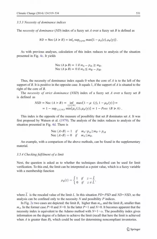
3.5.3 Necessity of dominance indices

The necessity of dominance (ND) index of a fuzzy set A over a fuzzy set B is defined as

As with previous analyses, calculation of this index reduces to analysis of the situationpresented in Fig. 4c. It yields

Thus, the necessity of dominance index equals 0 when the core of A is to the left of thesupport of B. It is positive in the opposite case. It equals 1, if the support of A is situated to theright of the core of B.

The necessity of strict dominance (NSD) index of a fuzzy set A over a fuzzy set Bis defined as

This index is the opposite of the measure of possibility that set B dominates set A. It wasfirst proposed by Watson et al. (1979). The analysis of the index reduces to analysis of thesituation presented in Fig. 4d. There is

Nec A≻Bð Þ ¼ 1 if mA−plA≥mB þ prBNec A≻Bð Þ ¼ 0 if mA≤mB:

An example, with a comparison of the above methods, can be found in the supplementarymaterial.

3.5.4 Checking fulfilment of a limit

Next, the question is asked as to whether the techniques described can be used for limitverification. To this end, the limit can be interpreted as a point value, which is a fuzzy variablewith a membership function

μB zð Þ ¼ 1 if z ¼ L̃0 if z ≠ L̃

;

�

where eL is the rescaled value of the limit L. In this situation PD=PSD and ND=NSD, so theanalysis can be confined only to the necessity N and possibility P indices.

In Fig. 2e two cases are depicted: the limit B1 higher than mA, and the limit B2 smaller thanmA. In the former case P>0 and N=0. In the latter P=1 and N>0. It becomes apparent that thenecessity index is equivalent to the Adamo method with N=1−α. The possibility index givesinformation on the degree of a failure to achieve the limit (recall that here the limit is achievedwhen A is greater than B), which could be used for determining noncompliant inventories.

Climatic Change (2014) 124:519–534 531

Thus, we can formulate the following rules. The inventory is considered compliant if thenecessity index is high enough. The inventory is considered noncompliant if the possibilityindex is small enough. This leads to the situation, which is fully analogous to the indecisioninterval in the probabilistic approach, as presented in Fig. 1e. Fixing the minimal necessity Nand maximal possibility P indices brings us to the notion of an indecision interval, where thenecessity index is too small and the possibility index is too high.

The application of the Dubois and Prade method provides useful information with respectto the compliance evaluation. Nevertheless, analysis of membership functions in three dimen-sions is rather cumbersome. Simple interpretations on the plane, as in Fig. 4, can help in theanalysis. Necessity indices give practically the same information as in the methods of Adamoand Nahorski et al. The possibility indices can be useful for quantifying noncompliance.

4 Conclusions

The paper presents the methods for the comparison of uncertain emission inventories, anddiscusses their usefulness for evaluation of emission reduction limits. The review shows avariety of approaches and techniques. It clearly demonstrates that the comparison of thereported inventories with no account of uncertainty distributions leads to paradoxes,and it is not well scientifically grounded. Some of the approaches, like the under-shooting method, have been proposed earlier (Godal et al. 2003; Nahorski et al. 2003;Jonas et al. 2010a), and adapted for emission trading, see additionally Nahorski et al.(2007); Nahorski and Horabik (2010, 2011). Any use of the techniques outlined in the papertakes uncertainty into account, see Table 1, and thus inevitably necessitates changes to thepresently used rules of compliance checking. To date, the verification mechanisms depend onlyon reported inventories. They give a decisive answer, which may, however, be difficult tosupport when uncertainty of the inventories is considered, as shown in Fig. 1. In terms ofprobability or other measures, like possibility, only weaker statements on compliance can beformulated; for example, the probability of not fulfilling the limit. This means that eitherconservative decisions have to be taken or indecision situations may occur. However, theselack any controversy and are thus transparent, since the inventories can be compared andordered. Ignoring uncertainty is more hazardous for asymmetric distributions, which may occurin many national inventories. It is also of great importance for comparisons of emissionuncertainty distributions representing sectors of different activities, such as energy andagriculture.

Within the fuzzy approach, some problems arise with the representation of the incompleteinformation on the inventories uncertainty in the form of membership functions. However, themembership functions can be constructed and interpreted as approximations to the inventoryuncertainty, formulated on the basis of the best available knowledge. The present state of thedevelopment in this area allows only weak statements on comparison to be formulated,providing only some indices of possibility or necessity for instance. For decision making,one can set critical values on these indices, however, it may be more difficult than for thestochastic case due to smaller intuition on the indices interpretation.

In spite of basic conceptual differences between the probabilistic and fuzzy approaches, manytechniques are surprisingly similar. Among them, the critical values and fuzzy dominancemethods provide similar techniques for checking compliance, with small technical differencesin terminology and decision parameters. This paper has not been intended to elaborate legislationpropositions for compliance rules, due in part to restrictions on its length. Examples of analyticalconditions for checking compliance can be found in the literature mentioned.

532 Climatic Change (2014) 124:519–534

Possible approximations of the uncertainty distributions in the fuzzy approach give rise tothe question of the impact of approximations on the final compliance condition. This issue isalso valid in the stochastic approach, since the required probability characteristics are not easyto be gathered by simple statistical treatment to get accurate estimates. It may be argued thatthis second-order uncertainty impacts the results to a lesser extent than the first-order uncer-tainty of the inventory itself. It seems that this question can be solved using the idea underlyingthe methods described in the present paper: the worse the data are, the lower the reportedinventory should be to achieve a sufficient credibility. Thorough investigation of this problemis left for further studies.

Acknowledgments O. Hryniewicz, Z. Nahorski and J. Verstraete gratefully acknowledge financial support fromthe Polish State Scientific Research Committee within the grant N N519316735 as well as from statutory fund ofthe Systems Research Institute. J. Horabik was financially supported by the Foundation for Polish Science underInternational PhD Projects in Intelligent Computing, which is financed by The European Union within theInnovative Economy Operational Programme 2007–2013 and European Regional Development Fund. Theauthors thank the anonymous reviewers for the comments, which helped us to improve the paper.

Open Access This article is distributed under the terms of the Creative Commons Attribution License whichpermits any use, distribution, and reproduction in any medium, provided the original author(s) and the source arecredited.

Table 1 Comparison of methods discussed in the paper

Group of methods Required information Characteristics and usefulness of the methods

Based on distributionmoments

Means and variances The methods use simple information but their applicationis rather inconvenient. Two indicators can contradicteach other. For asymmetric distributions, mean valuesare different from the reported (dominant) values.Application of semivariance requires information onthe uncertainty distribution.

Based on critical values Probability or possibilitymass of the inventoryuncertainty above aspecific value

This group of methods seems to be particularly convenientfor the compliance problem; some variants of thesemethods have been already proposed independently inseveral papers. The methods need more advancedinformation on the uncertainty distribution, whichrequires more sophisticated methods for its acquisition.Moreover, a good understanding of the applied inferencetechniques is required for decision making, as the valuesused in the compliance rules differ from the reportedinventories. This may be questioned on the ground ofdeterministic common-sense arguments.

Based on dominance Full distribution ofinventory uncertainty

Although the same notion of dominance is used in bothstochastic and fuzzy approaches, the methods are verydifferent. The stochastic methods are not always decisiveand rather difficult for practical applications. The fuzzymethods use little known notions of possibility andnecessity indices, and require understanding of thesophisticated underlying theory. The geometricalcalculation of the indices proposed in the present papermay make the method easier to grasp. As shown,comparison of an inventory against an exact (crisp) limitallows for its reduction to a variant of methods from thecritical values group.

Climatic Change (2014) 124:519–534 533

References

Adamo JM (1980) Fuzzy decision trees. Fuzzy Sets Syst 4:207–219Baas SM, Kwakernaak H (1977) Rating and ranking of multiple-aspect alternatives using fuzzy sets. Automatica

13:47–58Bortolan G, Degani R (1985) A review of some methods for ranking fuzzy subsets. Fuzzy Sets Syst 15:1–19Dubois D, Prade H (1983) Ranking fuzzy numbers in the setting of possibility theory. Inf Sci 30:183–224Gillenwater M, Sussman F, Cohen J (2007) Practical policy applications of uncertainty analysis for national

greenhouse gas inventories. Water, Air & Soil Pollution: Focus 7(4–5):451–474Godal O, Ermolev Y, Klaassen G, Obersteiner M (2003) Carbon trading with imperfectly observable emissions.

Environ Resour Econ 25:151–169Gusti M., Jęda W. (2002) Carbon management: new dimension of future carbon research. IR-02-006. IIASA,

Austria. http://www.iiasa.ac.at/Publications/Documents/IR-02-006.pdfGraves SB, Ringuest JL (2009) Probabilistic dominance criteria for comparing uncertain alternatives: A tutorial.

Omega 37:346–257Hryniewicz O., Nahorski Z. (2008) Verification of Kyoto Protocol - a fuzzy approach. In: L. Magdalena, M.

Ojeda-Aciego, J. L. Verdegay (Eds.) Proc. IPMU’08. Torremolinos, Spain, 729–734. http://www.gimac.uma.es/ipmu08/proceedings/papers/096-HryniewiczNahorski.pdf

IPCC (1996) Revised 1996 IPCC Guidelines for national Greenhouse Gas Inventories. Vol. 1. ReportingInstructions. IPCC. Available at: http://www.ipcc-nggip.iges.or.jp/public/gl/invs4.html

Jain R (1976) Decision-making in the presence of fuzzy variables. IEEE Trans Systems Man Cybernet 6:698–703

Jonas M, Nilsson S, Obersteiner M, Gluck M, Ermoliev YM (1999) Verification times underlying the Kyotoprotocol: Global benchmark calculations. IR-99-062. IIASA, Austria. http://www.iiasa.ac.at/Publications/Documents/IR-99-062.pdf

Jonas M, Nilsson S (2007) Prior to economic treatment of emissions and their uncertainties under the KyotoProtocol: Scientific uncertainties that must be kept in mind. Water, Air, and Soil Pollution: Focus 7:495–511

Jonas M, Gusti M, Jęda W, Nahorski Z, Nilsson S (2010a) Comparison of preparatory signal analysis techniquesfor consideration in the (post-)Kyoto policy process. Clim Chang 103(1–2):175–213

Jonas M, Marland G, Winiwarter W, White T, Nahorski Z, Bun R, Nilsson S (2010b) Benefits of dealing withuncertainty in greenhouse gas inventories: introduction. Clim Chang 103(1–2):3–18

Lieberman D, Jonas M, Winiwarter W, Nahorski Z, Nilsson S (eds) (2007) Accounting for climate change:Uncertainty in greenhouse gas inventories—verification, compliance, and trading. Springer, Dordrecht

Nahorski Z, Horabik J (2010) Compliance and emission trading: rules for asymmetric emission uncertaintyestimates. Clim Chang 103(1–2):303–325

Nahorski Z, Horabik J (2011) A market for pollution emission permits with low accuracy of emission estimates.In: Kaleta M, Traczyk T (eds) Modeling multi-commodity trade: Information exchange methods. Springer,Verlag, pp 151–165

Nahorski Z, Horabik J, Jonas M (2007) Compliance and emission trading under the Kyoto Protocol: Rules foruncertain inventories. Water, Air & Soil Pollution: Focus 7(4–5):539–558

Nahorski Z, Jęda W, Jonas M (2003) Coping with uncertainty in verification of the Kyoto obligations. In:Studziński J., Drelichowski L., Hryniewicz O. (Eds.) Zastosowania informatyki i analizy systemowej wzarządzaniu. SRI PASm, 305–317.

Ramirez RA, de Keizer C, van der Sluijs JP (2006) Monte Carlo analysis of uncertainties in the Netherlandsgreenhouse gas emission inventory for 1990–2004. Copernicus Institute for Sustainable Development andInnovation, Utrecht, the Netherlands. Available at: http://www.chem.uu.nl/nws/www/publica/publicaties2006/E2006-58.pdf

Roy AD (1952) Safety first and the holding of assets. Econometrica 20:431–449Tran L, Duckstein L (2002) Comparison of fuzzy numbers using a fuzzy distance measure. Fuzzy Sets Syst 130:

331–341Watson SR, Weiss JJ, Donell ML (1979) Fuzzy decision analysis. IEEE Trans Systems Man Cybernet 9:1–9White T, Jonas M, Nahorski Z, Nilsson S (eds) (2011) Greenhouse gas inventories. Dealing with uncertainty.

Springer, DordrechtWiniwarter W, Rypdal K (2001) Assessing the uncertainty associated with national greenhouse gas emission

inventories: A case study for Austria. Atmos Environ 35:5425–5440Yager RR (1981) A procedure for ordering fuzzy subsets of the unit interval. Inform Sci 24:143–161

534 Climatic Change (2014) 124:519–534